University of Groningen

Multiresolution volume processing and visualization on graphics hardwarevan der Laan, Wladimir

IMPORTANT NOTE: You are advised to consult the publisher's version (publisher's PDF) if you wish to cite fromit. Please check the document version below.

Document VersionPublisher's PDF, also known as Version of record

Publication date:2011

Link to publication in University of Groningen/UMCG research database

Citation for published version (APA):van der Laan, W. (2011). Multiresolution volume processing and visualization on graphics hardwareGroningen: s.n.

CopyrightOther than for strictly personal use, it is not permitted to download or to forward/distribute the text or part of it without the consent of theauthor(s) and/or copyright holder(s), unless the work is under an open content license (like Creative Commons).

Take-down policyIf you believe that this document breaches copyright please contact us providing details, and we will remove access to the work immediatelyand investigate your claim.

Downloaded from the University of Groningen/UMCG research database (Pure): http://www.rug.nl/research/portal. For technical reasons thenumber of authors shown on this cover page is limited to 10 maximum.

Download date: 25-06-2018

Wladimir J. van der Laan, Andrei C. Jalba, and Jos B.T.M. Roerdink. Accelerating Wavelet Lifting on GraphicsHardware using CUDA. IEEE Transactions on Parallel and Distributed Systems, 22, 2011, pp. 132-146.

Chapter 3

Accelerating Wavelet Lifting on GraphicsHardware using CUDA

3.1 IntroductionThe wavelet transform, originally developed as a tool for the analysis of seismic data, has beenapplied in areas as diverse as signal processing, video and image coding, compression, data min-ing and seismic analysis. The theory of wavelets bears a large similarity to Fourier analysis,where a signal is approximated by superposition of sinusoidal functions. A problem, however,is that the sinusoids have an infinite support, which makes Fourier analysis less suitable to ap-proximate sharp transitions in the function or signal. Wavelet analysis overcomes this problemby using small waves, called wavelets, which have a compact support. One starts with a waveletprototype function, called a basic wavelet or mother wavelet. Then a wavelet basis is constructedby translated and dilated (i.e., rescaled) versions of the basic wavelet. The fundamental idea isto decompose a signal into components with respect to this wavelet basis, and to reconstruct theoriginal signal as a superposition of wavelet basis functions; therefore we speak a multiresolutionanalysis. If the shape of the wavelets resembles that of the data, the wavelet analysis results ina sparse representation of the signal, making wavelets an interesting tool for data compression.This also allows a client-server model of data exchange, where data is first decomposed intodifferent levels of resolution on the server, then progressively transmitted to the client, wherethe data can be incrementally restored as it arrives (‘progressive refinement’). This is especiallyuseful when the data sets are very large, as in the case of 3D data visualization [148]. For somegeneral background on wavelets, the reader is referred to the books by Daubechies [28] or Mal-lat [84].

In the theory of wavelet analysis both continuous and discrete wavelet transforms are defined.If discrete and finite data are used it is appropriate to consider the Discrete Wavelet Transform(DWT). Like the discrete Fourier transform (DFT), the DWT is a linear and invertible transformthat operates on a data vector whose length is (usually) an integer power of two. The elementsof the transformed vector are called wavelet coefficients, in analogy of Fourier coefficients incase of the DFT. The DWT and its inverse can be computed by an efficient filter bank algorithm,called Mallat’s pyramid algorithm [84]. This algorithm involves repeated downsampling (for-ward transform) or upsampling (inverse transform) and convolution filtering by the application

26 3.1 Introduction

of high and low pass filters. Its complexity is linear in the number of data elements.In the construction of so-called first generation wavelet bases, which are translates and dilates

of a single basic function, Fourier transform techniques played a major role [28]. To deal withsituations where the Fourier transform is not applicable, such as wavelets on curves or surfaces, orwavelets for irregularly sampled data, second generation wavelets were proposed by Sweldens,based on the so-called lifting scheme [133]. This provides a flexible and efficient frameworkfor building wavelets. It works entirely in the original time/space domain, and does not involveFourier transforms.

The basic idea behind the lifting scheme is as follows. It starts with a simple wavelet, and thengradually builds a new wavelet, with improved properties, by adding new basis functions. So thesimple wavelet is lifted to a new wavelet, and this can be done repeatedly. Alternatively, onecan say that a complex wavelet transform is factored into a sequence of simple lifting steps [29].More details on lifting are provided in section 3.3.

Also for first generation wavelets, constructing them by the lifting scheme has a number ofadvantages [133]. First, it results in a faster implementation of the wavelet transform than thestraightforward convolution-based approach by reducing the number of arithmetic operations.Asymptotically for long filters, lifting is twice as fast as the standard algorithm. Second, giventhe forward transform, the inverse transform can be found in a trivial way. Third, no Fouriertransforms are needed. Lastly, it allows a fully in-place calculation of the wavelet transform,so no auxiliary memory is needed. With the generally limited amount of high-speed memoryavailable, and the large quantities of data that have to be processed in multimedia or visualizationapplications, this is a great advantage. Finally, the lifting scheme represents a universal discretewavelet transform which involves only integer coefficients instead of the usual floating pointcoefficients [16]. Therefore we based our DWT implementation on the lifting scheme.

Custom hardware implementations of the DWT have been developed to meet the compu-tational demands for systems that handle the enormous throughputs in, for example, real-timemultimedia processing. However, cost and availability concerns, and the inherent inflexibilityof this kind of solutions make it preferable to use a more widespread and general platform.NVidia’s G80 architecture [72], introduced in 2006 with the GeForce 8800 GPU, provides sucha platform. It is a highly parallel computing architecture available for systems ranging fromlaptops or desktop computers to high-end compute servers. In this chapter, we will present ahardware-accelerated DWT algorithm that makes use of the Compute Unified Device Architec-ture (CUDA) parallel programming model to fully exploit the new features offered by the G80architecture when compared to traditional GPU programming.

The three main hardware architectures for the 2D DWT, i.e., row-column, line-based, orblock-based, turn out to be unsuitable for a CUDA implementation (see Section 3.2). The biggestchallenge of fitting wavelet lifting in the SIMD model is that data sharing is, in principle, neededafter every lifting step. This makes the division into independent computational blocks difficult,and means that a compromise has to be made between minimizing the amount of data shared withneighbouring blocks (implying more synchronization overhead) and allowing larger data overlapin the computation at the borders (more computation overhead). This challenge is specificallydifficult with CUDA, as blocks cannot exchange data at all without returning execution flow tothe CPU. Our solution is a sliding window approach which enables us (in the case of separa-

Accelerating Wavelet Lifting on Graphics Hardware using CUDA 27

ble wavelets) to keep intermediate results longer in shared memory, instead of being written toglobal memory. Our CUDA-specific design can be regarded as a hybrid method between therow-column and block-based methods. We implemented our methods both for 2D and 3D data,and obtained considerable speedups compared to an optimized CPU implementation and earliernon-CUDA based GPU DWT methods. Additionally, memory usage can be reduced signifi-cantly compared to previous GPU DWT methods. The method is scalable and the fastest GPUimplementation among the methods considered. A performance analysis shows that the resultsof our CUDA-specific design are in close agreement with our theoretical complexity analysis.

The chapter is organized as follows. Section 3.2 gives a brief overview of GPU wavelet lift-ing methods, and previous work on GPU wavelet transforms. In Section 3.3 we present the basictheory of wavelet lifting. Section 3.4 first presents an overview of the CUDA programming envi-ronment and execution model, introduces some performance considerations for parallel CUDAprograms, and gives the details of our wavelet lifting implementation on GPU hardware. Section3.5 presents benchmark results and analyzes the performance of our method. Finally, in Section3.6 we draw conclusions and discuss future avenues of research.

3.2 Previous and related workIn [53] a method was first proposed that makes use of OpenGL extensions on early non-program-mable graphics hardware to perform the convolution and downsampling/upsampling for a 2-DDWT. Later, in [38] this was generalized to 3-D using a technique called tileboarding.

Wong et al. [158] implemented the DWT on programmable graphics hardware with the goalof speeding up JPEG2000 compression. They made the decision not to use wavelet lifting, basedon the rationale that, although lifting requires less memory and less computations, it imposesan order of execution which is not fully parallelizable. They assumed that lifting would requiremore rendering passes, and therefore in the end be slower than the standard approach based onconvolution.

However, Tenllado et al. [135] performed wavelet lifting on conventional graphics hardwareby splitting the computation into four passes using fragment shaders. They concluded that a gainof 10-20% could be obtained by using lifting instead of the standard approach based on convo-lution. Similar to [158], Tenllado et al. [136] also found that the lifting scheme implementedusing shaders requires more rendering steps, due to increased data dependencies. They showedthat for shorter wavelets the convolution-based approach yields a speedup of 50-100% comparedto lifting. However, for larger wavelets, on large images, the lifting scheme becomes 10-20%faster. A limitation of both [135] and [136] is that the methods are strictly focused on 2-D. It isuncertain whether, and if so, how they extend to three or more dimensions.

All previous methods are limited by the need to map the algorithms to graphics operations,constraining the kind of computations and memory accesses they could make use of. As we willshow below, new advances in GPU programming allow us to do in-place transforms in a singlepass, using intermediate fast shared memory.

Wavelet lifting on general parallel architectures was studied extensively in [61] for processornetworks with large communications latencies. A technique called boundary postprocessing

28 3.3 Wavelet lifting

was introduced that limits the amount of data sharing between processors working on individualblocks of data. This is similar to the technique we will use. More than in previous generationsof graphics cards, general parallel programming paradigms can now be applied when designingGPU algorithms.

The three main hardware architectures for the 2D DWT are row-column (RC), line-based(LB) and block-based (BB), see for example [1, 4, 20, 159], and all three schemes are based onwavelet lifting. The simplest one is RC, which applies a separate 1D DWT in both the horizontaland vertical directions for a given number of lifting levels. Although this architecture providesthe simplest control path (thus being the cheapest for a hardware realization), its major disadvan-tage is the lack of locality due to the use of large off-chip memory (i.e., the image memory), thusdecreasing performance. Contrary to RC, both LB and BB involve a local memory that operatesas a cache, thus increasing bandwidth utilization (throughput). On FPGA architectures, it wasfound [4] that the best instruction throughput is obtained by the LB method, followed by theRC and BB schemes which show comparable performances. As expected, both the LB and BBschemes have similar bandwidth requirements, which are at least two times smaller than that ofRC. Theoretical results [20, 159] show that this holds as well for ASIC architectures. Thus, LBis the best choice with respect to overall performance for a hardware implementation.

Unfortunately, a CUDA realization of LB is impossible for all but the shortest wavelets (e.g.,the Haar wavelet), due to the relatively large cache memory required. For example, the cachememory for the Deslauriers-Dubuc (13, 7) wavelet should accommodate six rows of the originalimage (i.e., 22.5 KB for two-byte word data and HD resolutions), well in excess of the maximumamount of 16 KB of shared memory available per multi-processor, see Section 3.4.3. As anefficient implementation of BB requires similar amounts of cache memory, this choice is againnot possible. Thus, the only feasible strategy remains RC. However, we show in Section 3.5 thateven an improved (using cache memory) RC strategy is not optimal for a CUDA implementation.Nevertheless, our CUDA-specific design can be regarded as a hybrid method between RC andBB, which also has an optimal access pattern to the slow global memory (see Section 3.4.1).

3.3 Wavelet liftingAs explained in the introduction, lifting is a very flexible framework to construct wavelets withdesired properties. When applied to first generation wavelets, lifting can be considered as areorganization of the computations leading to increased speed and more efficient memory usage.In this section we explain in more detail how this process works. First we discuss the traditionalwavelet transform computation by subband filtering and then outline the idea of wavelet lifting.

3.3.1 Wavelet transform by subband filteringThe main idea of (first generation) wavelet decomposition for finite 1-D signals is to start froma signal c0 = (c0

0, c01, . . . , c

0N−1), with N samples (we assume that N is a power of 2). Then we

apply convolution filtering of c0 by a low pass analysis filter H and downsample the result bya factor of 2 to get an “approximation” signal (or “band”) c1 of length N/2, i.e., half the initial

Accelerating Wavelet Lifting on Graphics Hardware using CUDA 29

length. Similarly, we apply convolution filtering of c0 by a high pass analysis filter G, followedby downsampling, to get a detail signal (or “band”) d1. Then we continue with c1 and repeat thesame steps, to get further approximation and detail signals c2 and d2 of length N/4. This processis continued a number of times, say J . Here J is called the number of levels or stages of thedecomposition. The explicit decomposition equations for the individual signal coefficients are:

cj+1k =

∑n

hn−2k cjn, d

j+1k =

∑n

gn−2k cjn

where {hn} and {gn} are the coefficients of the filtersH andG. Note that only the approximationbands are successively filtered, the detail bands are left “as is”.

This process is presented graphically in Fig. 3.1, where the symbol ↓2 (enclosed by a circle)indicates downsampling by a factor of 2. This means that after the decomposition the initial data

G 2

2H

G 2

2H

G 2

2H...c0 c1

d1

c2

d2

cJ

Jd

Figure 3.1. Structure of the forward wavelet transform with J stages: recursively split a signalc0 into approximation bands cj and detail bands dj .

vector c0 is represented by one approximation band cJ and J detail bands d1, d2, . . . , dJ . Thetotal length of these approximation and detail bands is equal to the length of the input signal c0.

Signal reconstruction is performed by the inverse wavelet transform: first upsample the ap-proximation and detail bands at the coarsest level J , then apply synthesis filters H and G tothese, and add the resulting bands. (In the case of orthonormal filters, such as the Haar basis,the synthesis filters are essentially equal to the analysis filters.) Again this is done recursively.This process is presented graphically in Fig. 3.2, where the symbol ↑2 indicates upsampling by afactor of 2.

2 H ~

2 G~

+ 2 H ~

2 G~

+ 2 H ~

2 G~

+...cJ

Jd

cJ−1

dJ−1

c1

d1

c0

Figure 3.2. Structure of the inverse wavelet transform with J stages: recursively upsample,filter and add approximation signals cj and detail signals dj .

3.3.2 Wavelet transform by liftingLifting consists of four steps: split, predict, update, and scale, see Fig. 3.3 (left).

30 3.3 Wavelet lifting

splitc UP

+

−

K

1/K

j+1even

j+1

odd

j+1c

j+1d

1/K

K

U P

+

−

jc

j+1

odd

j+1even

mergej

Figure 3.3. Classical lifting scheme (one stage only). Left part: forward lifting. Right part:inverse lifting. Here “split” is the trivial wavelet transform, “merge” is the opposite operation,P is the prediction step, U the update step, and K the scaling factor.

1. Split: this step splits a signal (of even length) into two sets of coefficients, those with evenand those with odd index, indicated by evenj+1 and oddj+1. This is called the lazy wavelettransform.

2. Predict lifting step: as the even and odd coefficients are correlated, we can predict onefrom the other. More specifically, a prediction operator P is applied to the even coefficientsand the result is subtracted from the odd coefficients to get the detail signal dj+1:

dj+1 = oddj+1 − P (evenj+1) (3.1)

3. Update lifting step: similarly, an update operator U is applied to the odd coefficients andadded to the even coefficients to define cj+1:

cj+1 = evenj+1 + U(dj+1) (3.2)

4. Scale: to ensure normalization, the approximation band cj+1 is scaled by a factor of K,and the detail band dj+1 by a factor of 1/K.

Sometimes the scaling step is omitted; in that case we speak of an unnormalized transform.A remarkable feature of the lifting technique is that the inverse transform can be found triv-

ially. This is done by “inverting” the wiring diagram, see Fig. 3.3 (right): undo the scaling, undothe update step (evenj+1 = cj+1−U(dj+1)), undo the predict step (oddj+1 = dj+1+P (evenj+1)),and merge the even and odd samples. Note that this scheme does not require the operators P andU to be invertible: nowhere does the inverse of P or U occur, only the roles of addition andsubtraction are interchanged. For a multistage transform the process is repeatedly applied to theapproximation bands, until a desired number of decomposition levels is reached. In the sameway as discussed in section 3.3.1, the total length of the decomposition bands equals that of theinitial signal. As an illustration, we give in Table 3.1 the explicit equations for one stage of theforward wavelet transform by the (unnormalized) Le Gall (5, 3) filter, both by subband filteringand lifting (in-place computation). It is easily verified that both schemes give identical resultsfor the computed approximation and detail coefficients.

Accelerating Wavelet Lifting on Graphics Hardware using CUDA 31

The process above can be extended by including more predict and/or update steps in thewiring diagram [133]. In fact, any wavelet transform with finite filters can be decomposed intoa sequence of lifting steps [29]. In practice, lifting steps are chosen to improve the decomposi-tion, for example, by producing a lifted transform with better decorrelation properties or highersmoothness of the resulting wavelet basis functions.

Wavelet lifting has two properties which are very important for a GPU implementation. First,it allows a fully in-place calculation of the wavelet transform, so no auxiliary memory is needed.Second, the lifting scheme can be modified to a transform that maps integers to integers [16].This is achieved by rounding the result of the P and U functions. This makes the predict andupdate operations nonlinear, but this does not affect the invertibility of the lifting transform.Integer-to-integer wavelet transforms are especially useful when the input data consists of integersamples. These schemes can avoid quantization, which is an attractive property for lossless datacompression.

For many wavelets of interest, the coefficients of the predict and update steps (before trunca-tion) are of the form z/2n, with z integer and n a positive integer. In that case one can implementall lifting steps (apart from normalization) by integer operations: integer addition and multipli-cation, and integer division by powers of 2 (bit-shifting).

Table 3.1. Forward wavelet transform (one stage only) by the (unnormalized) Le Gall (5, 3)filter.

Subband fil-tering

cj+1k = 1

8(−cj2k−2 + 2cj2k−1 + 6cj2k + 2cj2k+1 − c

j2k+2)

dj+1k = 1

2(−cj2k + 2cj2k+1 − c

j2k+2)

Lifting Split: cj+1k ← cj2k, dj+1

k ← cj2k+1

Predict: dj+1k ← dj+1

k − 12(cj+1k + cj+1

k+1)

Update: cj+1k ← cj+1

k + 14(dj+1k−1 + dj+1

k )

3.4 Wavelet lifting on GPUs using CUDA

3.4.1 CUDA overview

In recent years, GPUs have become increasingly powerful and more programmable. This combi-nation has led to the use of the GPU as the main computation device for diverse applications, suchas physics simulations, neural networks, image compression and even database sorting. The GPUhas moved from being used solely for graphical tasks to a fully-fledged parallel co-processor.Until recently, General Purpose GPU (GPGPU) applications, even though not concerned with

32 3.4 Wavelet lifting on GPUs using CUDA

graphics rendering, did use the rendering paradigm. In the most common scenario, texturedquadrilaterals were rendered to a texture, with a fragment shader performing the computation foreach fragment.

With their G80 series of graphics processors, NVidia introduced a programming environmentcalled CUDA [72]. It is an API that allows the GPU to be programmed through more traditionalmeans: a C-like language (with some C++-features such as templates) and compiler. The GPUprograms, now called kernels instead of shaders, are invoked through procedure calls insteadof rendering commands. This allows the programmer to focus on the main program structure,instead of details like color clamping, vertex coordinates and pixel offsets.

In addition to this generalization, CUDA also adds some features that are missing in shaderlanguages: random access to memory, fast integer arithmetic, bitwise operations, and sharedmemory. The usage of CUDA does not add any overhead, as it is a native interface to thehardware, and not an abstraction layer.

Execution model

The CUDA execution model is quite different from that of CPUs, and also different from thatof older GPUs. CUDA broadly follows the data-parallel model of computation [72]. The CPUinvokes the GPU by calling a kernel, which is a special C-function.

The lowest level of parallelism is formed by threads. A thread is a single scalar executionunit, and a large number of threads can run in parallel. The thread can be compared to a fragmentin traditional GPU programming. These threads are organized in blocks, and the threads of eachblock can cooperate efficiently by sharing data through fast shared memory. It is also possible toplace synchronization points (barriers) to coordinate operations closely, as these will synchronizethe control flow between all threads within a block. The Single Instruction Multiple Data (SIMD)aspect of CUDA is that the highest performance is realized if all threads within a warp of 32consecutive threads take the same execution path. If flow control is used within such a warp, andthe threads take different paths, they have to wait for each other. This is called divergence.

The highest level, which encompasses the entire kernel invocation, is called the grid. Thegrid consists of blocks that execute in parallel, if multiprocessors are available, or sequentially ifthis condition is not met. A limitation of CUDA is that blocks within a grid cannot communicatewith each other, and this is unlikely to change as independent blocks are a means to scalability.

Memory layout

The CUDA architecture gives access to several kinds of memory, each tuned for a specific pur-pose. The largest chunk of memory consists of the global memory, also known as device mem-ory. This memory is linearly addressable, and can be read and written at any position in any order(random access) from the device. No caching is done in G80, however there is limited cachingin the newest generation (GT200) as part of the shared memory can be configured as automaticcache. This means that optimizing access patterns is up to the programmer. Global memory isalso used for communication with the CPU, which can read and write using API calls. Registersare limited per-thread memory locations with very fast access, which are used for local storage.

Accelerating Wavelet Lifting on Graphics Hardware using CUDA 33

Shared memory is a limited per-block chunk of memory which is used for communication be-tween threads in a block. Variables are marked to be in shared memory using a specifier. Sharedmemory can be almost as fast as registers, provided that bank conflicts are avoided. Texture mem-ory is a special case of device memory which is cached for locality. Textures in CUDA work thesame as in traditional rendering, and support several addressing modes and filtering methods.Constant memory is cached memory that can be written by the CPU and read by the GPU. Oncea constant is in the constant cache, subsequent reads are as fast as register access.

The device is capable of reading 32-bit, 64-bit, or 128-bit words from global memory intoregisters in a single instruction. When access to device memory is properly distributed overthreads, it is compiled into 128-bit load instructions instead of 32-bit load instructions. Theconsecutive memory locations must be simultaneously accessed by the threads. This is calledmemory access coalescing [72], and it represents one of the most important optimizations inCUDA. We will confirm the huge difference in memory throughput between coalesced and non-coalesced access in our results.

3.4.2 Performance considerations for parallel CUDA programs (kernels)

Let us first define some metrics which we use later to analyze our results in Section 3.5.3 below.

Total execution time

Assume that a CUDA kernel performs computations on N data values, and organizes the CUDA‘execution model’ as follows. Let T denote the number of threads in a block, W the numberof threads in a warp, i.e., W = 32 for G80 GPUs, and B denote the number of thread blocks.Further, assume that the number of multiprocessors (device specific) is M , and that NVidia’soccupancy calculator [92] indicates that k blocks can be assigned to one multiprocessor (MP); kis program specific and represents the total number of threads for which (re)scheduling costs arezero, i.e., context switching is done with no extra overhead. Given that the amount of resourcesper MP is fixed (and small), k simply indicates the occupancy of the resources for the givenkernel. With this notation, the number of blocks assigned to one MP is given by b = B/M . Sincein general k is smaller than b, it follows that the number α of times k blocks are rescheduled isα =

⌈BMk

⌉.

Since each MP has 8 stream processors, a warp has 32 threads and there is no overheadwhen switching among the warp threads, it follows that each warp thread can execute one (arith-metic) instruction in four clock cycles. Thus, an estimate of the asymptotic time required by aCUDA kernel to execute n instructions over all available resources of a GPU, which also includesscheduling overhead, is given by

Te =4n

K

T

Wαk ls, (3.3)

where K is the clock frequency and ls is the latency introduced by the scheduler of each MP.The second component of the total execution time is given by the time Tm required to transfer

N bytes from global memory to fast registers and shared memory. If thread transfers of m bytes

34 3.4 Wavelet lifting on GPUs using CUDA

can be coalesced, given that a memory transaction is done per half-warp, it follows that thetransfer time Tm is

Tm =2N

W mMlm, (3.4)

where lm is the latency (in clock cycles) of a memory access. As indicated by NVidia [94],reported by others [146] and confirmed by us, the latency of a non-cached access can be as largeas 400 − 600 clock cycles. Compared to 24 cycle latency for accessing the shared memory, itmeans that transfers from global memory should be minimized. Note that for cached accessesthe latency becomes about 250− 350 cycles.

One way to effectively address the relatively expensive memory-transfer operations is byusing fine-grained thread parallelism. For instance, 24 cycle latency can be hidden by running 6warps (192 threads) per MP. To hide even larger latencies, the number of threads should be raised(thus, increasing the degree of parallelism) up to a maximum of 768 threads per MP supportedby the G80 architecture. However, increasing the number of threads while maintaining the sizeN of the problem fixed, implies that each thread has to perform less work. In doing so, oneshould still recall (i) the paramount importance of coalescing memory transactions and (ii) theFlops/word ratio, i.e., peak Gflop/s rate divided by global memory bandwidth in words [146],for a specific GPU. Thus, threads should not execute too few operations nor transfer too littledata, such that memory transfers cannot be coalesced. To summarize, a tradeoff should be foundbetween increased thread parallelism, suggesting more threads to hide memory-transfer latencieson the one hand, and on the other, memory coalescing and maintaining a specific Flops/wordratio, indicating fewer threads.

Let us assume that for a given kernel, one MP has an occupancy of k T threads. Further, if thekernel has a ratio r ∈ (0, 1) of arithmetic to arithmetic-and-memory-transfer instructions, andassuming a round-robin scheduling policy, then the reduction of memory-transfer latency due tolatency hiding is

lh =∑i≥0

⌊k T

8ri⌋. (3.5)

For example, assume that r = 0.5, i.e., there are as many arithmetic instructions (flops) asmemory transfers, and assume that k T = 768, i.e., each MP is fully occupied. The schedulerstarts by assigning 8 threads to a MP. Since r = 0.5 chances are that 4 threads execute each amemory transfer instruction while the others execute one arithmetic operation. After one cycle,those 4 threads executing memory transfers are still asleep for at least 350 cycles, while the othersjust finished executing the flop and are put to sleep too. The scheduler assigns now another 8threads, which again can execute either a memory transfer or a flop, with the same probability,and repeats the whole process. Counting the number of cycles in which 4 threads executedflops, reveals a number of 190 cycles, so that the latency is decreased in this way to just lm =350 − 190 = 160 cycles. In the general case, for a given r and occupancy, we postulate thatformula (3.5) applies.

The remaining component of the total GPU time for a kernel is given by the synchronizationtime. To estimate this component, we proceed as follows. Assume all active threads (i.e., k T ≤768) are about to execute a flop, after which they have to wait on a synchronization point (i.e.,

Accelerating Wavelet Lifting on Graphics Hardware using CUDA 35

on a barrier). Then, assuming again a round-robin scheduling policy and reasoning similar as forEq. (3.3), the idle time spent waiting on the barrier is

Ts =Ten

=4

K

T

Wαk ls. (3.6)

This agrees with NVidia’s remark that, if within a warp thread divergence is minimal, then wait-ing on a synchronization barrier requires only four cycles [94]. Note that the expression for Tsfrom Eq. (3.6) represents the minimum synchronization time, as threads were assumed to exe-cute (fast) flops. In the worst case scenario – at least one active thread has just started before thesynchronization point, a slow global-memory transaction – this estimate has to be multiplied bya factor of about 500/4 = 125 (the latency of a non-cached access divided by 4 threads).

To summarize, we estimate the total execution time Tt as Tt = Te + Tm + Ts.

Instruction throughput

Assuming that a CUDA kernel performs n flops in a number c of cycles, then the estimate ofthe asymptotic Gflop/s rate is Ge = 32M nK

c, whereas the measured Gflop/s rate is Gm = nN

Tt;

here K is the clock rate and Tt the (measured) total execution time. For the 8800 GTX GPU thepeak instruction throughput using register-to-register MAD instructions is about 338 Gflop/s anddrops to 230 Gflop/s when using transfers in/from shared memory [146].

Memory bandwidth

Another factor which should be taken into account when developing CUDA kernels is the mem-ory bandwidth,Mb = N

Tt. For example, parallel reduction has very low arithmetic intensity, i.e., 1

flop per loaded element, which makes it bandwidth-optimal. Thus, when implementing a parallelreduction in CUDA, one should strive for attaining peak bandwidth. On the contrary, if the prob-lem at hand is matrix multiplication (a trivial parallel computation, with little synchronizationoverhead), one should optimize for peak throughput. For the 8800 GTX GPU the pin-bandwidthis 86 GB/s.

Complexity

With coalesced accesses the number of bytes retrieved with one memory request (and thus onelatency) is maximized. In particular, coalescing reduces lm (through lh from Eq. 3.5) by a factorof about two. Hence one can safely assume that lm/(2W )→ 0. It follows that the total executiontime satisfies

Tt ∼ 4nN

W M D, (3.7)

where n is the number of instructions of a given CUDA kernel, N is the problem size, D is theproblem size per thread, and ∼ means that both left and right-hand side quantities have the sameorder of magnitude.

36 3.4 Wavelet lifting on GPUs using CUDA

The efficiency of a parallel algorithm is defined as

E =TSC

=TSM Tt

, (3.8)

where TS is the execution time of the (fastest) sequential algorithm, and C = M Tt is the costof the parallel algorithm. A parallel algorithm is called cost efficient (or cost optimal) if its costis proportional to TS . Let us assume TS ∼ nsN , where ns is the number of instructions forcomputing one data element and N denotes the problem size. Then, the efficiency becomes

E ∼ nsW D

4n. (3.9)

Thus, according to our metric above, for a given problem, any CUDA kernel which (i) usescoalesced memory transfers (i.e., lm/(2W ) → 0 is enforced), (ii) avoids thread divergence (sothat our Ts estimate from Eq. 3.6 applies), (iii) minimizes transfers from global memory, and (iv)has an instruction count n proportional to (nsW D) is cost efficient. Of course, the smaller n is,the more efficient the kernel becomes.

3.4.3 Parallel wavelet liftingEarlier parallel methods for wavelet lifting [61] assumed an MPI architecture with processors thathave their own memory space. However, the CUDA architecture is different. Each processor hasits own shared memory area of 16 KB, which is not enough to store a significant part of thedataset. As explained above, each processor is allocated a number of threads that run in paralleland can synchronize. The processors have no way to synchronize with each other, beyond theirinvocation by the host.

This means that data parallelism has to be used, and moreover, the dataset has to be splitinto parts that can be processed as independently as possible, so that each chunk of data can beallocated to a processor. For wavelet lifting, except for the Haar [133] transform, this task is nottrivial, as the implied data re-use in lifting also requires the coefficients just outside the delimitedblock to be updated. This could be solved by duplicating part of the data in each processor.Wavelet bases with a large support will however need more data duplication. If we want to do amultilevel transform, each level of lifting doubles the amount of duplicated work and data. Withthe limited amount of shared memory available in CUDA, this is not a feasible solution.

As kernel invocations introduce some overhead each time, we should also try to do as muchwork within one kernel as possible, so that the occupancy of the GPU is maximized. The slidingwindow approach enables us (in the case of separable wavelets) to keep intermediate resultslonger in shared memory, instead of being written to global memory.

3.4.4 Separable waveletsFor separable wavelet bases in 2-D it is possible to split the operation into a horizontal and avertical filtering step. For each filter level, a horizontal pass performs a 1-D transform on each

Accelerating Wavelet Lifting on Graphics Hardware using CUDA 37

Figure 3.4. Horizontal lifting step. h thread blocks are created, each containing T threads;each thread performs computations on N/(hT ) = w/T data. Black quads illustrate input forthe thread with id 0. Here w and h are the the dimensions of the input and N = w · h.

row, while a vertical pass computes a 1-D transform on each column. This lends itself to easyparallelization: each row can be handled in parallel during the horizontal pass, and then eachcolumn can be handled in parallel during the vertical pass. In CUDA this implies the use oftwo kernels, one for each pass. The simple solution would be to have each block process a rowwith the horizontal kernel, while in the vertical step each block processes a column. Each threadwithin these blocks can then filter an element. We will discuss better, specific algorithms for bothpasses in the upcoming subsections.

3.4.5 Horizontal passThe simple approach mentioned in the previous subsection works very well for the horizontalpass. Each block starts by reading a line into shared memory using so-called coalesced readsfrom device memory, executes the lifting steps in-place in fast shared memory, and writes backthe result using coalesced writes. This amounts to the following steps:

1. Read a row from device memory into shared memory.

2. Duplicate border elements (implement boundary condition).

3. Do a 1-D lifting step on the elements in shared memory.

4. Repeat steps 2 and 3 for each lifting step of the transform.

5. Write back the row to device memory.

As each step is dependent on the output in shared memory of the previous step, the threads withinthe block have to be synchronized every time before the next step can start. This ensures that theprevious step did finish and wrote back its work. Fig. 3.4 shows the configuration of the CUDAexecution model for the horizontal step. Without loss of generality, assume that N = w · h

38 3.4 Wavelet lifting on GPUs using CUDA

x0(0) x0(1) x0(3)x0(2)

x1(0)

x1(0) x1(1)y1(0) y1(1)

x1(1) y1(0) y1(1)

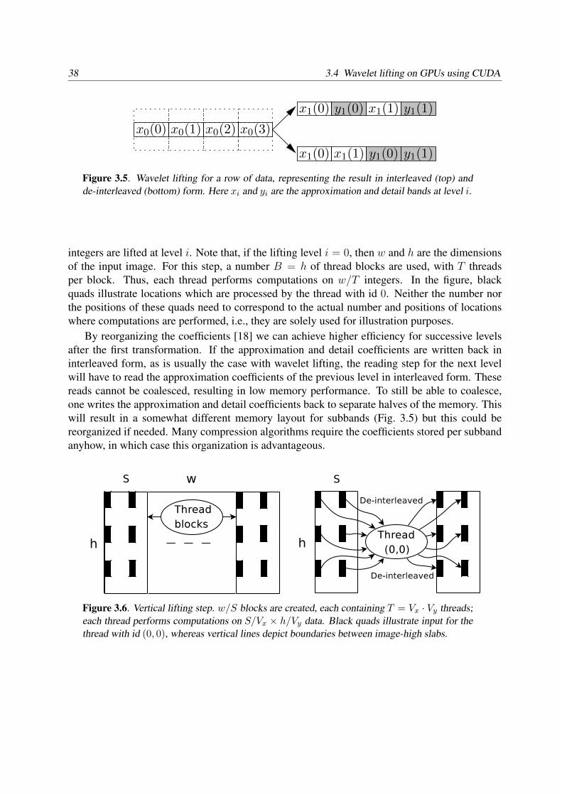
Figure 3.5. Wavelet lifting for a row of data, representing the result in interleaved (top) andde-interleaved (bottom) form. Here xi and yi are the approximation and detail bands at level i.

integers are lifted at level i. Note that, if the lifting level i = 0, then w and h are the dimensionsof the input image. For this step, a number B = h of thread blocks are used, with T threadsper block. Thus, each thread performs computations on w/T integers. In the figure, blackquads illustrate locations which are processed by the thread with id 0. Neither the number northe positions of these quads need to correspond to the actual number and positions of locationswhere computations are performed, i.e., they are solely used for illustration purposes.

By reorganizing the coefficients [18] we can achieve higher efficiency for successive levelsafter the first transformation. If the approximation and detail coefficients are written back ininterleaved form, as is usually the case with wavelet lifting, the reading step for the next levelwill have to read the approximation coefficients of the previous level in interleaved form. Thesereads cannot be coalesced, resulting in low memory performance. To still be able to coalesce,one writes the approximation and detail coefficients back to separate halves of the memory. Thiswill result in a somewhat different memory layout for subbands (Fig. 3.5) but this could bereorganized if needed. Many compression algorithms require the coefficients stored per subbandanyhow, in which case this organization is advantageous.

Figure 3.6. Vertical lifting step. w/S blocks are created, each containing T = Vx · Vy threads;each thread performs computations on S/Vx × h/Vy data. Black quads illustrate input for thethread with id (0, 0), whereas vertical lines depict boundaries between image-high slabs.

Accelerating Wavelet Lifting on Graphics Hardware using CUDA 39

3.4.6 Vertical pass

The vertical pass is more involved. Of course it is possible to use the same strategy as for thehorizontal pass, substituting rows for columns. But this is far from efficient. Reading a columnfrom the data would amount to reading one value per row. As only consecutive reads can becoalesced into one read, these are all performed individually. The processing steps would be thesame as for the horizontal pass, after which writing back is again very inefficient.

We can gain a 10 times speedup by using coalesced memory access. Instead of having eachblock process a column, we make each block process multiple columns by dividing the imageinto vertical “slabs”, see Fig. 3.6. Within a block, threads are organized into a 2D grid of sizeVx × Vy , instead of a 1D one, as in the horizontal step. The number S of columns in each slabis a multiple of Vx such that the resulting number of slab rows can still be coalesced, and has theheight of the image. Each thread block processes one of the slabs, i.e., S/Vx× h/Vy data. Usingthis organization, a thread can do a coalesced read from each row within a slab, do filtering inshared memory, and do a coalesced write to each slab row.

Another problem arises here, namely that the shared memory in CUDA is not large enoughto store all columns for any sizable dataset. This means that we cannot read and process theentire slab at once. The solution that we found is to use a sliding window within each slab,see Fig. 3.7(a). This window needs to have dimensions so that each thread in the block cantransform a signal element, and additional space to make sure that the support of the waveletdoes not exceed the top or bottom of the window. To determine the size of the window needed,how much to advance, and at which offset to start, we need to look at the support of each of thelifting steps.

In Fig. 3.7(a), height is the height of the working area. As each step updates either oddor even rows within a slab, each row of threads updates one row in each lifting step. Therefore,a good choice is to set it to two times the number of threads in the vertical direction. Similarly,width should be a multiple of the number of threads in the horizontal direction, and the size ofa row should be a multiple of the coalescable size. In the figure, rows in the top area have beenfully computed, while rows in the overlap area still need to go through at least one lifting step.The rows in the working area need to go through all lifting steps, whilst rows in the bottom areaare untouched except as border extension. The sizes of overlap, top and bottom depend onthe chosen wavelet. We will elaborate on this later.

The algorithm

Algorithm 3.1 shows the steps for the vertical lifting pass. Three basic operations are used: readcopies rows from device memory into shared memory, write copies rows from shared memoryback to device memory, and copy transfers rows from shared memory to another place in sharedmemory. The shared memory window is used as a cache, and to manage this we keep a read anda write pointer. The read pointer inrow indicates where to read from, the write pointer outrowindicates where to write back. After reading, we advance the read pointer, after writing weadvance the write pointer. Both are initialized to the top of the slab at the beginning of the kernel(line 1 and 2 of Algorithm 3.1).

40 3.4 Wavelet lifting on GPUs using CUDA

Bottom boundary

Top boundary

Overlap

Working area

width

top

overlap

bottom

heightWork area

Top

Bottom

Overlap

Top

Bottom

Work area

Overlap

(a) (b)

Figure 3.7. (a): The sliding window used during the vertical pass for separable wavelets. (b):Advancing the sliding window: the next window is aligned at the bottom of the previous one,taking the overlap area into account.

The first block has to be handled differently because we need to take the boundary conditionsinto account. So initially, rows are copied from the beginning of the slab to shared memory, fillingit from a certain offset to the end (line 5). Next we apply a vertical wavelet lifting transform(transformTop, line 7) to the rows in shared memory (it may be required to leave some rows atthe end untouched for some of the lifting steps, depending on their support; we will elaborate onthis in the next section). After this we write back the fully transformed rows from shared memoryto device memory (line 8). Then, for each block, the bottom part of the shared memory is copiedto the top part (Fig. 3.7(b)), in order to align the next window at the bottom of the previous one,taking the overlap area into account (line 11). The rest of the shared memory is filled again bycopying rows from the current read pointer of the slab (line 12).

Further, we apply a vertical wavelet lifting transform (transformBlock, line 14) to the rowsin the working area. This does not need to take boundary conditions into account as the topand bottom are handled specifically with transformTop and transformBottom. Then, heightrows are copied from shared memory row top to the current write pointer (line 15). This processis repeated until we have written back the entire slab, except for the last leftover part. Whenfinishing up (line 20), we have to be careful to satisfy the bottom boundary condition.

Example

We will discuss the Deslauriers-Dubuc (13, 7) wavelet as an example [31]. This example waschosen because it represents a non-trivial, but still compact enough case of the algorithm, that wecan go through step by step. The filter weights for the two lifting steps of this transform are shownin Table 3.2. Both the prediction and update steps depend on two coefficients before and after thesignal element to be computed. Fig. 3.8 shows an example of the performed computations. Forthis example, we choose top = 3, overlap = 2, height = 8 and bottom = 3. This is atoy example, as in practice height will be much larger when compared to the other parameters.

Starting with the first window at the start of the dataset, step 1 (first column), the odd rows

Accelerating Wavelet Lifting on Graphics Hardware using CUDA 41

Algorithm 3.1 The sliding window algorithm for the vertical wavelet lifting transform (see sec-tion 3.4.6). Here top, overlap, height, bottom are the length parameters of the slidingwindow (see Fig. 3.7), and h is the number of rows of the dataset. The pointer inrow indicateswhere to read from, the pointer outrow indicates where to write back.

1: inrow← 0 {initialize read pointer}2: outrow← 0 {initialize write pointer}3: windows← (h− height− bottom)/height {number of times window fits in slab}4: leftover← (h− height− bottom)%height {remainder}5: read(height+ bottom from row inrow to row top+ overlap) {copy from global to shared

memory}6: inrow← inrow + height + bottom {advance read pointer}7: transformTop() {apply vertical wavelet lifting to rows in shared memory}8: write(height− overlap from row top+ overlap to row outrow) {write transformed rows

back to global memory}9: outrow← outrow + height− overlap {advance write pointer}

10: for i = 1 to windows do {advance sliding window through slab and repeat above steps}11: copy(top + overlap + bottom from row height to row 0)12: read(height from row inrow to row top + overlap + bottom)13: inrow← inrow + height14: transformBlock() {vertical wavelet lifting}15: write(height from row top to row outrow)16: outrow← outrow + height17: end for18: copy(top + overlap + bottom from row height to row 0)19: read(leftover from row inrow to row top + overlap + bottom)20: transformBottom() {satisfy bottom boundary condition}21: write(leftover + overlap + bottom from row top to row outrow)

of the working area (offset 1, 3, 5, 7) are lifted. The lifted rows are marked with a cross, and therows they depend on are marked with a bullet. In step 2 (second column) the even rows are lifted.Again, the lifted rows are marked with a cross, and the dependencies are marked with a bullet.As the second step is dependent on the first, we cannot lift any rows that are dependent on valuesthat were not yet calculated in the last step. In Fig. 3.8, this would be the case for row 6: this rowrequires data in rows 3, 5, 7 and 9, but row 9 is not yet available.

Here the overlap region of rows comes in. As row 6 of the window is not yet fully trans-formed, we cannot write it back to device memory yet. So we write everything up to this rowback, copy the overlapping area to the top, and proceed with the second window. In the secondwindow, we again start with step 1. The odd rows are lifted, except for the first one (offset 7)which was already computed, i.e., rows 9, 11, 13 and 15 are lifted. Then, in step 2 we start atrow 6, i.e., three rows before the first step (row 9), but we do lift four rows.

After this we can write the top 8 rows back to device memory, and begin with the next windowin exactly the same way. We repeat this until the entire dataset is transformed. By letting thesecond lifting step lag behind the first, one can do the same number of operations in each, making

42 3.4 Wavelet lifting on GPUs using CUDA

Table 3.2. Filter weights of the two lifting steps for the Deslauriers-Dubuc (13, 7) [31] wavelet.The current element being updated is marked with •.

Offset Prediction Update

-3 − 116

-2 116

-1 916

0 − 916

•1 • 9

16

2 − 916

3 − 116

4 116

optimal use of the thread matrix (which should have a height of 4 in this case).All separable wavelet lifting transforms, even those with more than two lifting steps, or with

differently sized supports, can be computed in the same way. The transform can be inverted byrunning the steps in reverse order, and flipping the signs of the filter weights.

3.4.7 3-D and higher dimensions

The reason that the horizontal and vertical passes are asymmetric is because of the coalescingrequirement for reads and writes. In the horizontal case, an entire line of the data-set could beprocessed at a time. In the vertical case the data-set was horizontally split into image-high slabs.This allowed the slabs to be treated independently and processed using a sliding window algo-rithm that uses coalesced reads and writes to access lines of the slab. A consecutive, horizontalspan of values is stored at consecutive addresses in memory. This does not extend similarly tovertical spans of values, these will be separated by an offset at least the width of the image,known as the row pitch. As a slab is a rectangular region of the image of a certain width thatspans the height of the image, it will be represented in memory by an array of consecutive spansof values, each separated by the row pitch.

When adding an extra dimension, let us say z, the volume is stored as an array of slices. In aspan of values oriented along this dimension, each value is separated in memory by an offset thatwe call the slice pitch. By orienting the slabs in the xz-plane instead of the xy-plane, and thususing the slice pitch instead of the row pitch as offset between consecutive spans of values, thesame algorithm as in the vertical case can be used to do a lifting transform along this dimension.To verify our claim, we implemented the method just described, and report results in section3.5.2. More than three dimensions can be handled similarly, by orienting the slabs in the Dixplane (where Di is dimension i) and using the pitch in that dimension instead of the row pitch.

Accelerating Wavelet Lifting on Graphics Hardware using CUDA 43

012345678910

UpdatedDependency

78910111213141516

6

1718

543

Step Step

Off

set

Off

set

Overlap

Overlap

Bottom

Top

Bottom

1 2 1 2

First window Subsequent windows

Figure 3.8. The vertical pass for the Deslauriers-Dubuc (13, 7) [31] wavelet. Lifted rows ineach step are marked with a cross, dependent rows are marked with a bullet.

3.5 ResultsWe first present a broad collection of experimental results. This is followed by a performanceanalysis which provides insight in the results obtained, and also shows that the design choiceswe made closely match our theoretical predictions.

The benchmarks in this section were run on a machine with a AMD Athlon 64 X2 DualCore Processor 5200+ and a NVidia GeForce 8800 GTX 768MB graphics card, using CUDAversion 2.1 for the CUDA programs. All reported timings exclude the time needed for readingand writing images or volumes from and to disc (both for the CPU and GPU versions).

3.5.1 Wavelet filters used for benchmarkingThe wavelet filters that we used in our benchmarks are integer-to-integer versions (unnormal-ized) of the Haar [133], Deslauriers-Dubuc (9, 7) [31], Deslauriers-Dubuc (13, 7) [31], Le Gall(5, 3) [71], (integer approximation of) Daubechies (9, 7) [28] and the Fidelity wavelet – a customwavelet with a large support [9]. In the filter naming convention (m,n), m refers to the length ofthe analysis low-pass and n to the analysis high-pass filters in the conventional wavelet subbandfiltering model, in which a convolution is applied before subsampling. They do not reflect the

44 3.5 Results

length of the filters used in the lifting steps, which operate in the subsampled domain. The im-plementation only involves integer addition and multiplication, and integer division by powersof 2 (bit-shifting), cf. section 3.3.2. The coefficients of the lifting filters can be found in [9].

Table 3.3. Performance of our CUDA GPU implementation of 2D wavelet lifting (column5) compared to an optimized CPU implementation (column 2) and a CUDA GPU transposemethod (column 3, see text), computing a three-level decomposition of a 1920 × 1080 imagefor both analysis and synthesis steps.

Wavelet (analysis) CPU (ms) GPUtranspose(ms)

Speed-up GPU ourmethod(ms)

Speed-up

Haar 10.31 5.58 1.9 0.80 12.9Deslauriers-Dubuc (9, 7) 16.84 6.01 2.8 1.50 11.2Le Gall (5, 3) 14.03 5.89 2.4 1.34 10.5Deslauriers-Dubuc (13, 7) 19.52 6.08 3.2 1.62 12.0Daubechies (9, 7) 22.66 6.54 3.5 2.05 11.1Fidelity 28.82 6.45 4.5 2.11 13.7

Wavelet (synthesis) CPU (ms) GPUtranspose(ms)

Speed-up GPU ourmethod(ms)

Speed-up

Haar 9.11 6.33 1.4 0.83 11.0Deslauriers-Dubuc (9, 7) 15.93 6.40 2.5 1.45 11.0Le Gall (5, 3) 13.02 6.29 2.1 1.28 10.2Deslauriers-Dubuc (13, 7) 18.22 6.48 2.8 1.55 11.8Daubechies (9, 7) 21.73 7.03 3.1 2.04 10.7Fidelity 27.21 6.86 4.0 2.18 12.5

3.5.2 Experimental results and comparison to other methods

Comparison of 2D wavelet lifting, GPU versus CPU

First, we emphasize that the accuracies of the GPU and CPU implementations are the same.Because only integer operations are used (cf. section 3.5.1) the results are identical.

We compared the speed of performing various wavelet transforms using our optimized GPUimplementation, to an optimized wavelet lifting implementation on the CPU, called Schrodinger [9].The latter implementation makes use of vectorization using the MMX and SSE instruction setextensions, thus can be considered close to the maximum that can be achieved on the CPU withone core.

Accelerating Wavelet Lifting on Graphics Hardware using CUDA 45

Table 3.3 shows the timings of both our GPU accelerated implementation and the Schrodingerimplementation when computing a three-level transform with various wavelets of a 1920× 1080image consisting of 16-bit samples. As it is better from an optimization point of view to have atailored kernel for each wavelet type, than to have a single kernel that handles everything, we useda code generation approach to create specific kernels for the horizontal and vertical pass for eachof the wavelets. Both the analysis (forward) and synthesis (inverse) transform are benchmarked.We observe that speedups by a factor of 10 to 14 are reached, depending on the type of waveletand the direction of the transform. The speedup factor appears to be roughly proportional to thelength of the filters. The Haar wavelet is an exception, since the overlap problem does not arisein this case (the filter length being just 2), which explains the larger speedup factor.

To demonstrate the importance of coalesced memory access in CUDA, we also performedtimings using a trivial CUDA implementation of the Haar wavelet, that uses the same algorithmfor the vertical step as for the horizontal step, instead of our sliding window algorithm. Note thatthis method can be considered an improved (using cache) row-column, hardware-based strategy,see Section 3.2. Whilst our algorithm processes an image in 0.80 milliseconds, the trivial al-gorithm takes 15.23, which is almost 20 times slower. This is even slower than performing thetransformation on the CPU.

Note that the timings in Table 3.3 do not include the time required to copy the data from (2.4ms) or to (1.6 ms) the GPU.

Vertical step via transpose method

Another method that we have benchmarked consists in reusing the horizontal step as vertical stepby using a “transpose” method. Here, the matrix of wavelet coefficients is transposed after thehorizontal pass, the algorithm for the horizontal step is applied, and the results are transposedback. The results are shown in columns 3 and 4 of Table 3.3. Even though the transpose op-eration in CUDA is efficient and coalescable, and this approach is much easier to implement,the additional passes over the data reduce performance quite severely. Another drawback ofthis method is that transposition cannot be done in-place efficiently (in the general case), whichdoubles the required memory, so that the advantage of using the lifting strategy is lost.

Comparison of horizontal and vertical steps

Table 3.4 shows separate benchmarks for the horizontal and vertical steps, using various waveletfilters. From these results one can conclude that the vertical pass is not significantly slower (andin some cases even faster) than the horizontal pass, even though it performs more elaborate cachemanagement, see Algorithm 3.1.

Timings for 16-bit versus 32-bit integers

We also benchmarked an implementation that uses 32-bit integers, see Table 3.5. For smallwavelets like Haar, the timings for 16- and 32-bit differ by a factor of around 1.5, whereas forlarge wavelets the two are quite close. This is probably because the smaller wavelet transforms

46 3.5 Results

Table 3.4. Performance of our GPU implementation on 16-bit integers, separate timings ofhorizontal and vertical steps on a one-level decomposition of a 1920× 1080 image.

Wavelet (analysis) Horizontal (ms) Vertical (ms)

Haar 0.26 0.19Deslauriers-Dubuc (9, 7) 0.44 0.42Le Gall (5, 3) 0.39 0.34Deslauriers-Dubuc (13, 7) 0.47 0.47Daubechies (9, 7) 0.62 0.62Fidelity 0.63 0.76

Wavelet (synthesis) Horizontal (ms) Vertical (ms)

Haar 0.29 0.19Deslauriers-Dubuc (9, 7) 0.39 0.44Le Gall (5, 3) 0.35 0.36Deslauriers-Dubuc (13, 7) 0.42 0.48Daubechies (9, 7) 0.58 0.79Fidelity 0.59 0.64

Table 3.5. Performance of our GPU implementation on 16 versus 32-bit integers (3 level trans-form, 1920× 1080 image).

Wavelet (analysis) 16-bit (ms) 32-bit (ms)

Haar 0.80 1.09Deslauriers-Dubuc (9, 7) 1.50 1.64Le Gall (5, 3) 1.34 1.45Deslauriers-Dubuc (13, 7) 1.62 1.75Daubechies (9, 7) 2.05 2.13Fidelity 2.11 2.72

Wavelet (synthesis) 16-bit (ms) 32-bit (ms)

Haar 0.83 1.15Deslauriers-Dubuc (9, 7) 1.45 1.81Le Gall (5, 3) 1.28 1.66Deslauriers-Dubuc (13, 7) 1.55 1.90Daubechies (9, 7) 2.04 2.35Fidelity 2.18 2.80

Accelerating Wavelet Lifting on Graphics Hardware using CUDA 47

256 512 1024 2048 4096Image size in both dimensions (pixels)

0.1

1.0

10.0

100.0

1000.0Tim

e (

ms)

CPUTenlladoOur method

0 500 1000 1500 2000 2500 3000 3500 4000 4500Image size in both dimensions (pixels)

0

5

10

15

20

25

30

35

40

45

Tim

e (

ms)

TenlladoOur method

Figure 3.9. Computation time versus image size for various lifting implementations; 3-levelDaubechies (9, 7) forward transform. Top: the Schrodinger CPU implementation, Tenlladoet al. [136] and our CUDA accelerated method in a log-log plot. Bottom: just the two GPUmethods in a linear plot.

48 3.5 Results

are more memory-bound and the larger wavelets are more compute-bound, hence the increasedmemory bandwidth does not affect the performance significantly.

Comparison of 2D wavelet lifting on GPU, CUDA versus fragment shaders

We also implemented the algorithm of Tenllado et al. [136] for wavelet lifting using conven-tional fragment shaders and performed timings on the same hardware. A three-level Daubechies(9, 7) forward wavelet transform was applied to a 1920× 1080 image, which took 5.99 millisec-onds. In comparison, our CUDA-based implementation (see Table 3.3) does the same in 2.05milliseconds, which is about 2.9 times faster. This speedup probably occurs because our methodeffectively makes use of CUDA shared memory to compute intermediate lifting steps, conserv-ing GPU memory bandwidth, which is the bottleneck in the Tenllado method. Another drawbackthat we noticed while implementing the method is that an important advantage of wavelet lifting,i.e., that it can be done in place, appears to have been ignored. This is possibly due to an OpenGLrestriction by which it is not allowed to use the source buffer as destination, the same result isachieved by alternating between two halves of a buffer, resulting in a doubling of memory usage.

Figure 3.9 further compares the performance of the Schrodinger CPU implementation, Ten-llado et al. [136] and our CUDA accelerated method. A three-level Daubechies (9, 7) forwardwavelet decomposition was applied to images of different sizes, and the computation time wasplotted versus image size in a log-log graph. This shows that our method is faster by a constantfactor, regardless of the image size. Even for smaller images, our CUDA accelerated implemen-tation is faster than the CPU implementation, whereas the shader-based method of Tenllado isslower for 256×256 images, due to OpenGL rendering and state set-up overhead. CUDA kernelcalls are relatively lightweight, so this problem does not arise in our approach. For larger imagesthe overhead averages out, but as the method is less bandwidth efficient it remains behind by asignificant factor.

Comparison of lifting versus convolution in CUDA

Additionally, we compared our method to a convolution-based wavelet transform implemented inCUDA, one that uses shared memory to perform the convolution plus downsampling (analysis),or upsampling plus convolution (synthesis) efficiently. On a 1920 × 1080 image, for a three-level transform with the Daubechies (9, 7) wavelet, the following timings are observed: 3.4ms for analysis and 5.0 ms for synthesis. The analysis is faster than the synthesis because itrequires less computations – only half of the coefficients have to be computed, while the otherhalf is discarded in the downsampling step. Compared to the 2.0 ms of our own method for bothtransforms, this is significantly slower. This matches the expectation that a speedup factor of 1.5to 2 can be achieved when using lifting [133].

Timings for 3D wavelet lifting in CUDA

Timings for the 3-D approach outlined in Section 3.4.7 are given in Table 3.6. A three-leveltransform was applied to a 5123 volume, using various wavelets. The timings are compared to

Accelerating Wavelet Lifting on Graphics Hardware using CUDA 49

Table 3.6. Performance of our GPU lifting implementation in 3D, compared to an optimizedCPU implementation; a three-level decomposition for both analysis and synthesis is performed,on a 5123 volume.

Wavelet (analysis) CPU (ms) GPU (ms) Speed-up

Haar 1037.4 147.2 7.0Deslauriers-Dubuc (9, 7) 2333.1 192.0 12.2Le Gall (5, 3) 1636.2 179.3 9.1Deslauriers-Dubuc (13, 7) 3056.1 200.5 15.2Daubechies (9, 7) 3041.3 234.6 13.0Fidelity 5918.4 239.2 24.7

Wavelet (synthesis) CPU (ms) GPU (ms) Speed-up

Haar 926.5 150.9 6.1Deslauriers-Dubuc (9, 7) 2289.9 184.7 12.4Le Gall (5, 3) 1631.1 173.7 9.4Deslauriers-Dubuc (13, 7) 2983.9 192.1 15.5Daubechies (9, 7) 2943.5 232.0 12.7Fidelity 5830.7 230.9 25.3

the same CPU implementation as before, extended to 3-D. The numbers show that the speed-upsthat can be achieved for higher dimensional transforms are considerable, especially for the largerwavelets such as Deslauriers-Dubuc (13, 7) or Fidelity.

Summary of experimental results

Compared to an optimized CPU implementation, we have seen performance gains of up to nearly14 times for 2D and up to 25 times for 3D images by using our CUDA based wavelet liftingmethod. Especially for the larger wavelets, the gains are substantial. When compared to thetrivial transpose-based method our method came out about two times faster over the entire spec-trum of wavelets. When regarding computation time versus image size, our GPU based waveletlifting method was measured to be the fastest of three methods for all image sizes, with the factormostly independent of the image size.

3.5.3 Performance AnalysisWe analyze the performance of our GPU implementation, according to the metrics from Sec-tion 3.4.2, for performing one lifting (analysis) step. Without loss of generality, we discuss theDeslauriers-Dubuc (13, 7) wavelet, cf. Section 3.4.6. Our systematic approach consists first inexplaining the total execution time, throughput and bandwidth of our method, and then in dis-cussing the design decisions we made. The overhead of data transfer between CPU and GPU

50 3.5 Results

was excluded, since the wavelet transform is usually part of a larger processing pipeline (such asa video codec), of which multiple steps can be carried out on the GPU.

Horizontal step

The size of the input data set is N = w · h = 1920 · 1080 two-byte words. We set T = 256threads per block, and given the number of registers and the size of the shared memory used byour kernel, NVidia’s occupancy calculator indicates that k = 3 blocks are active per MP, suchthat each MP is fully occupied (i.e., k T = 768 threads will be scheduled); the number of threadblocks for the horizontal step is B = 1080. Given that the 8800 GTX GPU has M = 16 MPsit follows that α = 23, see Section 3.4.2. Further, we used decuda (a disassembler of GPUbinaries; see http://wiki.github.com/laanwj/decuda) to count the number and type of instructionsperformed. After unrolling the loops, we found that the kernel has 309 instructions, 182 ofwhich are arithmetic operations in local memory and registers, 15 instructions are half-width(i.e., instruction code is 32-bit wide), 82 are memory transfers and 30 are other instructions(mostly type conversions). Assuming that half-width instructions have a throughput of 2 cycles,and others take 4 cycles per warp, and since the clock rate of this device is K = 1.35 GHz, theasymptotic execution time is Te = 0.48 ms. Here we assumed that the extra overhead due torescheduling is negligible, as was confirmed by our experiments.

For the transfer time, we first computed the ratio of arithmetic to arithmetic-and-transfersinstructions, which is r = 0.67. Thus, from Eq. (3.5) it follows that as many as 301 cycles can bespared due to latency hiding. As the amount of shared memory used by the kernel is relativelysmall (i.e., 3 × 3.75 KB used out of 16 KB per MP) and the size of the L2 cache is about 12KB per MP [146], we can safely assume that the latency of a global memory access is about 350cycles, so that lm = 49 cycles. Sincem = 4 (i.e., two two-byte words are coalesced), the transfertime is Tm = 0.15 ms. Note that as two MPs also share a small but faster L1 cache of 1.5 KB, thereal transfer time could be even smaller than our estimate. Moreover, as we included also in ourcounting shared-memory transfers (whose latency is at least 10 times smaller than that of globalmemory), the real transfer time should be much smaller than its estimate.

According to our discussion in Section 3.4.5, five synchronization points are needed to ensuredata consistency between individual steps. For one barrier, in the ideal case, the estimated waitingtime is Ts = 1.65 µs, thus the total time is about 8.25 µs. In the worst case Ts = 0.2 ms, so thatthe total time can be as large as 1 ms.

To summarize, the estimated execution time for the horizontal step is about Tt = 0.63 ms, ne-glecting the synchronization time. Comparing this result with the measured one from Table 3.4,one sees that the estimated total time is 0.16 ms larger than the measured one. Probably this isdue to L1 caching contributing to a further decrease of Tm. However, essential is that the to-tal time is dominated by the execution time, indicating a compute-bound kernel. As the timingremains essentially the same (cf. Tables 3.3 and 3.5) when switching from two-byte words tofour-byte words data, this further strengthens our finding.

The measured throughput is Gm = 98 Gflop/s, whereas the estimated one is Ge = 104Gflop/s, indicating on average an instruction throughput of about 100 Gflop/s. Note that withsome abuse of terminology we refer to flops, when in fact we mean arithmetic instructions on in-

Accelerating Wavelet Lifting on Graphics Hardware using CUDA 51

tegers. The measured bandwidth is Mb = 8.8 GB/s, i.e., we are quite far from the pin-bandwidth(86 GB/s) of the GPU, thus one can conclude again that our kernel is indeed compute-bound. Thisconclusion is further supported by the fact that the flop-to-byte ratio of the GPU is 5, while inour case this ratio is about 11. The fact that the kernel does not achieve the maximum throughput(using shared memory) of about 230 Gflop/s is most likely due to the fact that the synchronizationtime cannot simply be neglected and seems to play an important role in the overall performance.

Let us now focus on the design choices we have made. Using T = 256 threads per blockamounts to optimal time slicing (latency hiding), see discussion above and in Section 3.4.2,while we are still able to coalesce memory transfers. To decrease the synchronization time,lighter threads are suggested implying that their number should increase, while maintaining afixed size of the problem. NVidia’s performance guidelines [94] suggest that the optimal numberof threads per block should be a multiple of 64. The next higher than 256 multiple of 64 is 320.Unfortunately, using 320 threads per block means that at most two blocks can be allocated to oneMP, and thus the MP will not be fully occupied. This in turn implies that an important amount ofidle cycles spent on memory transfers cannot be saved, rendering the method less optimal withrespect to time slicing. Accordingly, our choice of T = 256 threads per block is optimal. Further,our choice on the number of blocks also fulfills NVidia’s guidelines with respect to current andfuture GPUs, see [94].

Vertical step

While conceptually more involved than the horizontal step, the overall performance figure forthe vertical step is rather similar to the horizontal one. The CUDA configuration for this kernelis as follows. Each 2D thread block contains a number of 16 × 8 = 128 threads, while thenumber of columns within each slab is S = 32, see Figure 3.6. Thus, since the input consists oftwo-byte words, each thread performs coalesced memory transfers of m = 4 bytes, similar to thehorizontal step. As the number of blocks is w/S = 60, k = 4 (i.e., four blocks are scheduled perMP), and the kernel takes 39240 cycles per warp to execute, the execution time for the verticalstep is Te = 0.46.

Unlike the horizontal step, now r = 0.83 so that no less than 352 cycles can be spared inglobal-memory transaction. Note that when computing r we only counted global-memory trans-fers, as in this case more, much faster shared-memory transfers take place, see Algorithm 3.1. Asthe shared-memory usage is only 4×1.8 KB, this suggests that the overhead due to slow accessesto global memory can be neglected, so that the transfer time Tm can be neglected. The waitingtime is Ts = 0.047 µs, and there are 344 synchronization points for the vertical-step kernel, sothat the total time is about 15.6 µs. In the worst case, this time can be as large as 1.9 ms. Thus, asTt = 0.46 (without waiting time), our estimate is very close to the measured execution time fromTable 3.4 – this being in turn the same as that of the horizontal step. Finally, both the measuredand estimated throughputs are comparable to their counterparts of the horizontal step.

Note that compared to the manually-tuned, optimally-designed matrix-multiplication algo-rithm of [146] which is able to achieve a maximum throughput of 186 Gflop/s, the performanceof 100 Gflop/s of our lifting algorithms may not seem impressive. However, one should keepin mind that matrix-multiplication is much easier to parallelize efficiently, as it requires little

52 3.6 Conclusion

synchronization. Unlike matrix-multiplication, the lifting algorithm requires a lot more synchro-nization points to ensure data consistency between steps, as the transformation is done in-place.

The configuration we chose for this kernel is 16× 8 = 128 threads per block and w/S = 60thread blocks. This results in an occupancy of 512 threads per MP, which may seem less optimal.However, to increase the number of threads per block to 192 (next larger multiple of 64, seeabove), would mean that either we cannot perform essential, coalesced memory accesses, orthat extra overhead due to the requirements of the moving-window algorithm would have to beaccommodated. Note that we verified this possibility, but the results were unsatisfactory.

Complexity

Based on the formulae from Section 3.4.2 we can analyze the complexity of our problem. Forany of the lifting steps using the Deslauriers-Dubuc (13, 7) wavelet, considering that the numberof flops per data element is ns = 22 (20 multiply or additions and 2 register-shifts to increaseaccuracy), the numerator of (3.9) becomes about 700D. For the horizontal step, D = w/T =7.5, so that the numerator becomes about 5000. In this case the number of cycles is about1250, so that one can conclude that the horizontal step is indeed cost efficient. For the verticalstep, D = (S h)/T = 270, so that the numerator in (3.9) becomes about 190000, while thedenominator is 39240. Thus, the vertical step is also cost efficient, and actually its performanceis similar to that of the horizontal step (because 5000/1250 ≈ 190000/39240 ≈ 5). Of course,this result was already obtained experimentally, see Table 3.4. Note that using vectorized MMXand SSE instructions, the optimized CPU implementation (see Table 3.3) can be up to four timesfaster than our TS estimate above. However, even in this case, both our CUDA kernels are stillcost-efficient. Obviously both steps are also work efficient, as their CUDA realizations do notperform asymptotically more operations than the sequential algorithm.

3.6 ConclusionWe presented a novel, fast wavelet lifting implementation on graphics hardware using CUDA,which extends to any number of dimensions. The method tries to maximize coalesced memoryaccess. We compared our method to an optimized CPU implementation of the lifting scheme,to another (non-CUDA based) GPU wavelet lifting method, and also to an implementation ofthe wavelet transform in CUDA via convolution. We implemented our method both for 2D and3D data. The method is scalable and was shown to be the fastest GPU implementation amongthe methods considered. Our theoretical performance estimates turned out to be in fairly closeagreement with the experimental observations. The complexity analysis revealed that our CUDAkernels are cost- and work-efficient.

Our proposed GPU algorithm can be applied in all cases were the Discrete Wavelet Transformbased on the lifting scheme is part of a pipeline for processing large amounts of data. Examplesare the encoding of static images, such as the wavelet-based successor to JPEG, JPEG2000 [124],or video coding schemes [9], which we already considered in [143].