University of Groningen Equivalence of switching linear ...

University of Groningen

Equivalence of switching linear systems by bisimulationPola, G.; Schaft, A.J. van der; Benedetto, M.D. Di

Published in:International Journal of Control

IMPORTANT NOTE: You are advised to consult the publisher's version (publisher's PDF) if you wish to cite fromit. Please check the document version below.

Document VersionPublisher's PDF, also known as Version of record

Publication date:2006

Link to publication in University of Groningen/UMCG research database

Citation for published version (APA):Pola, G., Schaft, A. J. V. D., & Benedetto, M. D. D. (2006). Equivalence of switching linear systems bybisimulation. International Journal of Control, 79(1), 74-92.

CopyrightOther than for strictly personal use, it is not permitted to download or to forward/distribute the text or part of it without the consent of theauthor(s) and/or copyright holder(s), unless the work is under an open content license (like Creative Commons).

Take-down policyIf you believe that this document breaches copyright please contact us providing details, and we will remove access to the work immediatelyand investigate your claim.

Downloaded from the University of Groningen/UMCG research database (Pure): http://www.rug.nl/research/portal. For technical reasons thenumber of authors shown on this cover page is limited to 10 maximum.

Download date: 12-11-2019

brought to you by COREView metadata, citation and similar papers at core.ac.uk

provided by University of Groningen

https://core.ac.uk/display/232460844?utm_source=pdf&utm_medium=banner&utm_campaign=pdf-decoration-v1

https://www.rug.nl/research/portal/en/publications/equivalence-of-switching-linear-systems-by-bisimulation(d37426f9-0b9d-4f23-9885-2203c46d8ffc).html

International Journal of Control

Vol. 79, No. 1, January 2006, 74–92

Equivalence of switching linear systems by bisimulation

G. POLA*{, A. J. VAN DER SCHAFT{and M. D. DI BENEDETTO{

{Department of Electrical Engineering and Computer Science, Center of Excellence DEWS,University of L’Aquila, Poggio di Roio, 67040 L’Aquila, Italy,{Department of Applied Mathematics, University of Twente,

P.O. Box 217,7500 AE Enschede, The Netherlands

(Received 11 November 2004; in final form 27 September 2005)

A general notion of hybrid bisimulation is proposed for the class of switching linear systems.

Connections between the notions of bisimulation-based equivalence, state-space equivalence,

algebraic and input–output equivalence are investigated. An algebraic characterization of

hybrid bisimulation and an algorithmic procedure converging in a finite number of steps to

the maximal hybrid bisimulation are derived. Hybrid state space reduction is performed

by hybrid bisimulation between the hybrid system and itself. By specializing the results

obtained on bisimulation, also characterizations of simulation and abstraction are derived.

Connections between observability, bisimulation-based reduction and simulation-based

abstraction are studied.

1. Introduction

Hybrid systems have been the subject of intense research

over the past few years because of their expressive power

that is able to capture various non-smooth phenomena

in diverse application areas. Furthermore, many

interesting theoretical problems arise from the analysis

and design of these systems. However in many situations

the resulting hybrid systems are very complex, both in

scale and in dynamical properties. Therefore the task

of analysis and of synthesizing hybrid controllers to

ensure some prescribed performances requirements is a

complicated one, and formal methods for complexity

reduction are essential for a feasible approach to the

study of hybrid systems.

A powerful tool in this context, is the theory of

bisimulation, introduced in the 1980s by Milner (1989)

and Park (1981). This theory often provides an effective

method for reducing the complexity of concurrent pro-

cesses. The key idea in the notion of bisimulation is to

find (and compute) an equivalence relation on the

class of hybrid systems under consideration that is pre-

serving the properties of interest. Then reduction is per-

formed by choosing the minimal (in the sense of size of

state space) system in the sub-class of dynamical systems

belonging to the same equivalence class of this bisimula-

tion relation.

In the context of concurrent processes, the partition

of the state space into equivalence classes induced by

the bisimulation relation is in general finer than

the partition induced by input–output equivalence or

trace equivalence (Only for deterministic systems trace

equivalence can be shown to imply bisimulation

equivalence).

Also in system and control theory various equivalence

notions have been formulated for continuous systems

such as state-space and input–output equivalence.

Developments in both areas have been rather

independent; one of the reasons being that the employed

mathematics are rather different. The rise of interest in

hybrid systems has led to a reapproachment of the equiva-

lence notions on concurrent processes developed in the

computer science community with the equivalence

notions for continuous systems in the control community.*Corresponding author. Email: [email protected]

International Journal of Control

ISSN 0020–7179 print/ISSN 1366–5820 online ß 2006 Taylor & Francis

http://www.tandf.co.uk/journals

DOI: 10.1080/00207170500380839

Dow

nlo

aded

by [

Univ

ersi

ty o

f G

ronin

gen

] at

05:4

5 1

0 F

ebru

ary 2

012

In particular, extensions of the notion of bisimulation to

continuous systems have been explored before in

Broucke (1998) and in a series of papers by Pappas and

co-authors (e.g. Henzinger (1995), Lafferriere et al.

(1998, 2000), Alur et al. (2000), Tabuada et al. (2002)

and Pappas (2003, 2004)). The common denominator of

those works is to associate a transition system with

uncountable discrete state space to the continuous

systemunder consideration, preserving reachability prop-

erties. Then, after reduction by bisimulation a simpler

transition system is obtained, which hopefully has a

finite discrete state space, thereby allowing the use of stan-

dard methods for analysis and verification of concurrent

systems. This problem is not decidable in general as

shown in Alur et al. (2000). However, by restricting the

class of hybrid systems to timed automata, multirate

automata, rectangular automata and O-minimal hybrid

systems (Tabuada et al. 2002), the reduced transition

system is finite. The continuous systems considered in

Henzinger (1995), Lafferriere et al. (1998, 2000), Alur

et al. (2000) and Tabuada et al. (2002) neither have

continuous inputs or continuous outputs. Recently

Pappas et al. proposed a new definition of bisimulation

for linear (Pappas 2003, Tabuada et al. 2003, ) and non-

linear (Pappas 2004) systems that do include continuous

control inputs. In particular Pappas (2003) derives for

the case of linear control systems, interesting connections

between the maximal bisimulation relation and the

maximal controlled invariant subspace contained in the

kernel of a given observation map, while Pappas (2004)

shows how to reduce non-linear control systems

to lower-dimensional systems by factoring out certain

invariant distributions.

While in the previous approach the emphasis is on the

preservation of the reachability properties, van der

Schaft (2004a, b, c) focuses on external equivalence as

the key property to be preserved in the definition of

bisimulation. This latter approach is fundamental to a

compositional modelling and control of hybrid systems

as argued in van der Schaft and Schumacher (2001). In

particular, it allows the design of a controller applied

to the original continuous system on the basis of the

reduced dynamical system. Furthermore in van der

Schaft (2004a, c) it is shown that a linear deterministic

dynamical system � is observable if and only if it

equals the minimal system that is bisimilar to �,

thus offering interesting links between the theory of

bisimulation, the theory of realization, and the classical

Kalman decomposition.

The aim of the present paper is to make another

step in the reapproachement between the theory of

concurrent processes and mathematical systems theory

by defining and studying the notion of bisimulation

for continuous-time switching linear systems. A switch-

ing linear system (SLS) (De Santis et al. 2003) can be

viewed as a combination of a discrete event (concurrent)

system with linear continuous dynamical systems and

includes as external variables both continuous inputs

and outputs, discrete outputs, as well as hybrid (discrete

and continuous) disturbance variables. These hybrid

disturbances may be thought of as internal generators

for non-determinism. The resulting class of systems are

rather general since they may accept Zeno executions

(Lygeros 1999), are non-deterministic, since a hybrid

disturbance acts on the plant, and a reset map is defined

over the set of continuous states.

Inspired by classical notions of bisimulation for

concurrent processes (Clarke et al. 2002) and by the

new notions introduced in (van der Schaft 2004a, c)

for linear and non-linear dynamical systems, we propose

a general notion of hybrid bisimulation for the class of

switching linear systems. Given a pair of SLSs S1 and

S2, the proposed definition formalizes the intuitive

idea of finding a relation R � �1 ��2 between the

hybrid spaces �1 and �2 of S1 and S2 such that for

any continuous input u and for any pair of initial condi-

tions in R, R is invariant and the hybrid outputs coin-

cide for any time and for a suitable choice of the

hybrid disturbances. The proposed definition does not

make use of the particular semantics of the class of

SLSs involving only the notion of execution, and there-

fore may be also applied to more general hybrid systems

where for example the discrete transitions depend on the

continuous state x of the automata. A first step in this

direction has been made in (van der Schaft 2004a, b).

Moreover the definition applies to SLSs where multiple

instantaneous jumps are allowed and where any execu-

tion �1 of an SLS S1 may be mimicked by an execution

�2 of an SLS S2 and vice versa, while the jumps of �1and �2 may be asynchronous (compare with the

definition employed in (van der Schaft 2004a, b)).

The proposed definition seems particularly appealing

since it has clear links to well-known notions of

algebraic, state-space and input–output equivalences

(Callier and Desoer 1991) for dynamical systems. In

fact bisimulation-based equivalence will be shown to

be implied by algebraic equivalence, while implying

state-space equivalence and input–output equivalence.

Summarizing, we will prove the following sequence of

implications:

Algebraic E:)Bisimilarity) StateÿSpace E:

) InputÿOutput E:

The proposed equivalence notions, except for algebraic

equivalence, all coincide for the class of deterministic

SLSs (no hybrid disturbances). By combining tools

from concurrent systems analysis and from geometric

control theory, a complete geometric characterization

of hybrid bisimulations is derived. Moreover, inspired

Equivalence of switching linear systems 75

Dow

nlo

aded

by [

Univ

ersi

ty o

f G

ronin

gen

] at

05:4

5 1

0 F

ebru

ary 2

012

by De Santis et al. (2004a), an algorithmic procedure

converging in a finite number of steps to the maximal

hybrid bisimulation is developed. This yields the con-

struction of the minimal-dimensional SLS bisimilar to

the original one. By specializing those results we propose

a new definition of simulation that, roughly speaking, is

a one-sided version of the notion of bisimulation, lead-

ing to a notion of abstraction for the class of SLSs.

Inspired by the connections between bisimulation and

observability for linear continuous systems (van der

Schaft 2004a, b), we also investigate this issue in the

context of SLSs. In view of the results developed in

De Santis et al. (2003), that characterize observability

of SLSs, we show that while an observable SLS

cannot be reduced anymore by bisimulation, the con-

verse implication is not true. More precisely, an example

is provided where an SLS that cannot be reduced by

bisimulation, is unobservable. Finally we use simula-

tion-based abstraction, instead of bisimulation-based

reduction for ‘extracting’ the observable sub-SLS of a

given unobservable SLS.

Most of the results presented in this paper also hold for

the class of discrete-time switching linear systems.

Moreover even if most of the bisimulation analysis will

be carried out in the context of switching linear

systems, it may be naturally extended to the case of

switching non-linear systems, in view of the results of

van der Schaft (2004c), and to the case of switching

systems with continuous dynamics given in pencil form

in view of the results developed in van der Schaft

(2004b), aswill be briefly discussed in the end of the paper.

A preliminary and partial version of this paper has

been published as (Pola et al. 2004).

The paper is organized as follows. In x 2, a general

notion of hybrid bisimulation is proposed and charac-

terized, and relations to equivalence notions are given.

In x 3, an algorithmic procedure converging in a finite

number of steps to the maximal hybrid bisimulation is

proposed. In x 4, reduction via bisimulation is studied.

x 5 is devoted to the definition and characterization of

simulation and abstraction. Section 6 addresses the

issue of connections between observability, reduction

via bisimulation, and abstraction via simulation. x 7

offers some guidelines for extending the results obtained

for switching linear systems to the case of switching non-

linear systems and switching systems in pencil form. The

Appendix contains some technical proofs. Finally, x 8

offers some concluding remarks.

2. Bisimilar switching linear systems

2.1. Preliminaries and basic definitions

Switching systems are an important subclass of hybrid

systems that have been extensively studied in the past

few years (e.g. Wicks et al. (1998), Zefran and Burdick

(1998), Dayawansa and Martin (1999), De Santis et al.

(2003, 2004b, 2005) and Pola et al. (2004)). The motiva-

tion for considering this particular subclass of hybrid

systems lies in their semantics that is able to capture

different non-smooth phenomena, arising in the area

of mechanical systems, power train control, aircraft

and air traffic control, switching power converters and

many other fields (e.g. Wicks et al. (1998), Zefran

and Burdick (1998), Dayawansa and Martin (1999),

de Santis et al. (2005) and the references therein). For

example in (De Santis et al. 2005), an automotive

engine in idle mode is modelled by means of a suitable

switching system, where times of switchings between

the different modes are lower bounded and upper

bounded by two positive real parameters that depend

themselves on the engine parameters. The hybrid state

� of a switching linear system is composed of two com-

ponents: the discrete state q belonging to a finite set Q

and the continuous state x belonging to a linear space

X(q) depending on q. The evolution of the discrete

state is governed by a discrete disturbance v that acts

on the plant, while the evolution of x is given by a

non-deterministic linear dynamical control system

whose matrices depend on the current discrete state q.

Whenever a discrete transition holds, the continuous

state is instantly reset to a new value by means of a

reset matrix depending on the discrete states before

and after the transition. Moreover switching linear sys-

tems are characterized by a hybrid output y associated

to the hybrid state � and allow multiple instantaneous

transitions on the discrete states. The formal model of

a switching linear system is given in the following defini-

tion that is based on (De Santis et al. 2003), following

the general model of hybrid automata, see e.g.

(Tomlin et al. 1998) and (Lygeros et al. 1999).

Definition 1: A Switching Linear System (SLS) S is a

tuple ð�,U,D,Y, �, ,E,M Þ where

. � ¼ [q2Qfqg � XðqÞ is the hybrid state space, where

– Q ¼ fq1, q2, . . . , qN1g is the discrete state space,

N1 2 N,

– dim: Q!N,

– 8q 2 Q,XðqÞ � RdimðqÞ is the linear continuous state

space.. U is the linear input space.. D ¼ V�W is the hybrid disturbance space, where

– V ¼ fv1, v2, . . . , vN2g is the set of the discrete distur-

bances, N2 2 N,

– W is the linear continuous disturbance space.. Y ¼ P�H is the hybrid output space, where

– P ¼ fp1, p2, . . . , pN3g is the discrete output space,

N3 2 N,

– H is the linear continuous output space.

76 G. Pola et al.

Dow

nlo

aded

by [

Univ

ersi

ty o

f G

ronin

gen

] at

05:4

5 1

0 F

ebru

ary 2

012

. � is a function that associates to any discrete state

q 2 Q, the linear dynamical system

�ðqÞ:_xxðtÞ ¼ AðqÞxðtÞ þ BðqÞuðtÞ þ GðqÞwðtÞ,

hðtÞ ¼ CðqÞxðtÞ, t � 0:

�

. : Q ! P associates a discrete output to each discrete

state.. E � Q� V�Q is a collection of discrete transitions.. M is a function that associates to any e ¼ ðq, v, q 0Þ 2

E, the reset matrix MðeÞ 2 RdimðqÞ�dimðq 0Þ.

Any element � ¼ ðq, xÞ 2 � is called hybrid state, any

element d ¼ ðv,wÞ 2 D is called hybrid disturbance and

any element y ¼ ð p, hÞ 2 Y is called hybrid output of

S. Given an SLS S, the tuple DS ¼ ðQ,P,V,E, Þ can

be viewed as a Discrete Event System (DES) (Hopcroft

and Ullman 1979), having state space Q, output set P,

input set V, transition relation E and output function

. The set succðqÞ is composed by the successors of the

discrete state q 2 Q, i.e. succðqÞ ¼ fq 0 2 Q j 9v 2 V:

ðq, v, q 0Þ 2 Eg. Given a set Z � Z1 � Z2, the operator

�jZiðZÞ is the projection of the set Z onto Zi, i ¼ 1, 2.

We now formally define the semantics of switching

linear systems. First of all we assume throughout

the paper that the hybrid disturbance is not available

for measurements, thus yielding a non-deterministic

system.

The discrete transitions in the class of SLSs are

determined by the discrete disturbance v. We assume

that multiple events (instantaneous transitions) are

allowed. This can be formalized by using the notion

of hybrid time basis proposed in (Lygeros et al. 1999).

We recall that a hybrid time basis � is an infinite or

finite sequence of time intervals Ij, j 2 f0, 1, . . . , Jg,

i.e. � ¼ fIjgJj¼0, J 2 N [ f1g, satisfying the following

conditions:

. Ij ¼ ft 2 Rþ0 : tj � t � t 0j g, if j< J;

. IJ may be of the form ft 2 Rþ0 : tJ � t � t 0Jg or of the

form ft 2 Rþ0 : tJ � t < 1g and t 0J ¼ 1;

. for all j, tj � t 0j and for j>0, tj ¼ t 0jÿ1.

Denote by T the set of all hybrid time bases. Since the

SLSs under consideration are time-invariant continuous

systems, there is no loss of generality in assuming t0 ¼ 0,

for all � 2 T . Given a hybrid time basis � 2 T , denote by

½�� :¼ [Ij2�Ij � fjg the set of all hybrid times (t, j), t 2 Ij,

Ij 2 �, and define the ordering relation � on ½�� such

that ðt, jÞ � ðt 0, j 0Þ if t � t 0 and j � j 0. Given two hybrid

time bases �1, �2 2 T , such that supft : ðt, jÞ 2 ½�1�g ¼

supft : ðt, jÞ 2 ½�2�g denote by ½�1, �2� � ½�1� � ½�2� any

relation, satisfying the following conditions:

. �j½�i�ð½�1, �2�Þ ¼ ½�i�, i ¼ 1, 2;

. 8ððta, jaÞ, ðtb, jbÞÞ 2 ½�1, �2�, ta ¼ tb;

. 8ððta, jaÞ, ðtb, jbÞÞ, ððt0a, j

0aÞ, ðt

0b, j

0bÞÞ 2 ½�1, �2�, if ðta, jaÞ �

ðt 0a, j0aÞ then ðtb, jbÞ � ðt 0b, j

0bÞ and vice versa.

Remark 1: The last condition ensures that any

relation ½�1, �2� preserves the ordering relation� in

every hybrid time basis ½�1� and ½�2�.

Given two sets Z1, Z2, denote by CðZ1,Z2Þ and by

C0ðZ1,Z2Þ the class of functions, respectively of piece-

wise continuous functions z: Z1 ! Z2. The switching

system temporal evolution is then defined by means of

the notion of execution.

Definition 2: An execution � of an SLS S is a collec-

tion ð�0, �, u, d, �, yÞ with �0 ¼ ðq0, x0Þ 2 �, � 2 T , u 2

C0ðRþ0 ,UÞ, d ¼ ðv,wÞ, where v 2 CðN,V Þ,w 2 C0ðRþ

0 ,

WÞ, � ¼ ðq, xÞ, where q 2 CðN,QÞ, x 2 CðRþ0 �N,

Xð�ÞÞ, y ¼ ð p, hÞ, where p 2 CðN,PÞ, h 2 CðRþ0 �N,HÞ,

such that, by setting �ðt, jÞ ¼ ðqð j Þ, xðt, jÞÞ and yðt, jÞ ¼

ð pð j Þ, hðt, jÞÞ, for all ðt, jÞ 2 ½��, the following conditions

are satisfied:

. Discrete evolution: qð j Þ ¼ q0; q jþ 1ð Þ is such that

ej ¼ ðq jð Þ, vð jþ 1Þ, q ð jþ 1ÞÞ 2 E; pð j Þ ¼ ðqð j ÞÞ;. Continuous evolution: x t0, 0ð Þ ¼ x0, xðtjþ1, jþ 1Þ ¼

Mðejþ1Þxðt0j , jÞ; moreover xðt, jÞ and hðt, jÞ, for all

t 2 Ij are respectively the unique solution and output

at time t of the dynamical system �ðqð j ÞÞ, with initial

state x tj, j Þÿ

, initial time tj, input function u and

disturbance function w.

Switching linear systems are non-deterministic since a

hybrid disturbance acts on the plant: note that even

if the discrete disturbance would be measured then

still the dynamics of the discrete variables could be

non-deterministic.

We now introduce some equivalence notions,

borrowed from the theory of concurrent processes, for

the class of SLSs. In particular we consider the notions

of bisimulation and simulation for SLSs. The proposed

definitions are obtained by merging the classical notions

for concurrent processes (e.g. Clarke et al. (2002))

with new definitions introduced in van der Schaft

(2004a, c) for the classes of linear and non-linear contin-

uous systems.

Definition 3: Consider two SLSs Si ¼ ð�i,Ui,Di,Yi,

�i, i,Ei,MiÞ, i ¼ 1, 2 such that U1 ¼ U2. A hybrid

bisimulation between S1 and S2 is a subset R � �1�

�2 satisfying the following property. Take any ð�10, �20Þ

2 R and any input function u1 ¼ u2. Then for any

hybrid disturbance d1 and for any execution �1 ¼

ð�10, �1, u1, d1, �1, y1Þ of S1, there should exist a hybrid

disturbance d2 and an execution �2 ¼ ð�20, �2, u2, d2,

�2, y2Þ of S2 satisfying the following conditions:

(i) ð�1ðt, jÞ, �2ðt0, j 0ÞÞ 2 R,

(ii) y1ðt, jÞ ¼ y2ðt0, j 0Þ,


Dow

nlo

aded

by [

Univ

ersi

ty o

f G

ronin

gen

] at

05:4

5 1

0 F

ebru

ary 2

012

8ððt, jÞ, ðt 0, j 0ÞÞ 2 ½�1, �2�, for some ½�1, �2�. Moreover the

same holds with d1 replaced by d2 and vice versa.

Remark 2: The introduction of the relation ½�1, �2�

allows the comparison of the hybrid state and output

time-evolutions of the executions �1 and �2 with

different hybrid time bases �1 and �2, thus generalizing

the definition of structural hybrid bisimulation

introduced in (van der Schaft 2004a, b), where �1 ¼ �2was required, and where multiple instantaneous jumps

were not considered.

Definition 4: Two SLSs S1 and S2 are bisimilar, and

we write S1 � S2, if there exists a hybrid bisimulation

R � �1 ��2 such that the projection of R on each

hybrid space equals this hybrid space, i.e.

�j�iðRÞ ¼ �i, i ¼ 1, 2: ð1Þ

Remark 3: The notion of bisimulation equivalence in

the context of concurrent processes is usually given

with respect to an initial state; on the contrary

Definition 4 is given with respect to any hybrid initial

state. The generalization to subsets of initial conditions

�0i � �i, i ¼ 1, 2 obviously can be done by relaxing (1)

to �j�iðRÞ ¼ �0

i , i ¼ 1, 2.

We recall that, given a set Z, a set R � Z� Z is an

equivalence relation on Z if it is reflexive, i.e.

8z 2 Z, ðz, zÞ 2 R, symmetric, i.e. 8ðz1, z2Þ 2 R, ðz1, z2Þ 2

R, and transitive, 8ðz1, z2Þ, ðz2, z3Þ 2 R, ðz1, z3Þ 2 R.

Bisimilarity between SLSs is an equivalence relation

on the space of SLSs. A weaker notion than bisimula-

tion is the so-called notion of simulation, as formalized

hereafter.

Definition 5: Consider two SLSs Si ¼ ð�i,Ui,Di,Yi,

�i, i,Ei,MiÞ, i¼ 1, 2 such that U1 � U2. A hybrid

simulation of S1 by S2 is a subset R � �1 ��2 satisfy-

ing the following property. Take any �10, �20ð Þ 2 R and

any input function u1 ¼ u2. Then for any hybrid distur-

bance d1 and for any execution �1 ¼ ð�10, �1, u1, d1, �1, y1Þ

of S1, there should exist a hybrid disturbance d2 and an

execution �2 ¼ ð�20, �2, u2, d2, �2, y2Þ of S2 satisfying the

following conditions:

(i) �1ðt, jÞ, �2ðt0, j 0Þð Þ 2 R;

(ii) y1ðt, jÞ ¼ y2ðt0, j 0Þ;

8ððt, jÞ, ðt 0, j 0ÞÞ 2 ½�1, �2�, for some ½�1, �2�:

Definition 6: An SLS S1 is simulated by an SLS S2 (or

equivalently S2 simulates S1), and we write S1 4S2,

if there exists a hybrid simulation R � �1 ��2 of

S1 by S2 such that the projection of R along

the hybrid space �1 coincides with �1, i.e.

�j�1ðRÞ ¼ �1.

Hybrid simulation is reflexive, transitive but not

symmetric, and hence it is not an equivalence relation

on the space of SLSs. An equivalence notion based on

hybrid simulations can be stated as follows.

Definition 7: Two SLSs S1 and S2 are similar if S1 4

S2 and S2 4S1.

2.2. Equivalent switching linear systems

Equivalence notions in the control theory usually deal

with the characterization of whether two dynamical

systems are state-space equivalent or input–output

equivalent. Aim of this section is to define those

notions for the class of SLSs and then to compare

them with the notions of bisimilarity and similarity.

The following definition extends to the class of

SLSs well known concepts of algebraic, state-

space and input–output equivalence for linear continu-

ous systems (Callier and Desoer 1991) and DESs

(Clarke et al. 2002).

Definition 8: Two SLSs S1 and S2 are algebraically

equivalent if there exists an invertible mapping

TQ: Q1 ! Q2 and for any q1 2 Q1, invertible linear

mappings Tq1 : X1ðq1Þ ! X2ðTQðq1ÞÞ such that,

(i) 1ðq1Þ ¼ 2ðTQðq1ÞÞ, for any q1 2 Q1;

(ii) for any e1 ¼ ðq1, v1, q01Þ 2 E1, there exists v2 2 V2

such that e2 ¼ ðTQðq1Þ, v2,TQðq01ÞÞ 2 E2 and vice

versa;

(iii) for any q1 2 Q1, the dynamical systems �1ðq1Þ

and �2ðTQðq1ÞÞ are algebraically equivalent

(Callier and Desoer 1991) with transformation

matrix Tq1 , i.e.

A1ðq1Þ ¼ Tq1A2ðTQðq1ÞÞTÿ1q1

,

B1ðq1Þ ¼ Tq1B2ðTQðq1ÞÞ,

G1ðq1Þ ¼ Tq1G2ðTQðq1ÞÞ,

C1ðq1Þ ¼ C2ðTQðq1ÞÞTÿ1q1

,

(iv) M1ðe1Þ ¼ Tÿ1q 01M2ðe2ÞTq1 , for any e1 ¼ ðq1, v1, q

01Þ 2

E1, where e2 ¼ ðTQðq1Þ, v2, TQðq01ÞÞ 2 E2, for some

v2 2 V2, and vice versa.

A notion of equivalence that is less conservative than

algebraic equivalence is the notion of state-space

equivalence as formalized below. This can be obtained

by generalizing the corresponding notion given in

(Callier and Desoer 1991) for linear continuous systems.

Definition 9: Let S1 and S2 be two (not necessarily

distinct) SLSs with the same continuous control space,

i.e. U1 ¼ U2. Two hybrid states �10 2 �1 and �20 2 �2

are said to be state-equivalent if for any given input u,

for any hybrid disturbance d1, for any execution

�1 ¼ ð�10, �1, u, d1, �1, y1Þ of S1, there exists a hybrid

78 G. Pola et al.

Dow

nlo

aded

by [

Univ

ersi

ty o

f G

ronin

gen

] at

05:4

5 1

0 F

ebru

ary 2

012

disturbance d2 and an execution �2 ¼ ð�20, �2, u, d2,

�2, y2Þ of S2 such that y1ðt, jÞ ¼ y2ðt0, j 0Þ, 8ððt, jÞ,

ðt 0, j 0ÞÞ 2 ½�1, �2�, for some ½�1, �2�. Moreover the same

holds with d1 replaced by d2 and vice versa.

Definition 10: Two SLSs S1 and S2 are state-space

equivalent if they have the same continuous input

space, i.e. U1 ¼ U2 and for any hybrid state �1 2 �1 of

S1, there exists a hybrid state �2 2 �2 of S2 that is

equivalent to �1, and vice versa.

The following result highlights the connection between

state-space equivalence and bisimilarity.

Lemma 1: Two SLSs S1 and S2 are state-

space equivalent if and only if there exists a relation

R � �1 ��2 such that �j�iðRÞ ¼ �i, i¼ 1, 2 and

such that for any ð�10, �20Þ 2 R, �10 and �20 are state-

equivalent.

Another important equivalence notion in the context of

control theory is the notion of input–output equivalence

as given below.

Definition 11: Two SLSs S1 and S2 are input–output

equivalent if U1 ¼ U2 and for any �10 2 �1, for any

given control law u 2 U1, for any hybrid disturbance

d1, for any execution �1 ¼ ð�10, �1, u, d1, �1, y1Þ of S1,

there exists �20 2 �2, a hybrid disturbance d2 and an

execution �2 ¼ ð�20, �2, u, d2, �2, y2Þ of S2 such that

y1ðt, jÞ ¼ y2ðt0, j 0Þ, 8ððt, jÞ, ðt 0, j 0ÞÞ 2 ½�1, �2�, for some

½�1, �2�. Moreover the same holds with �10 and d1replaced by �20 and d2 and vice versa.

The above notions naturally specialize to the context of

DESs (Clarke et al. 2002) and linear dynamical systems

(Callier and Desoer 1991, van der Schaft 2004c). In

particular in the context of DESs, algebraic equivalence

is usually known as graph isomorphism and input–

output equivalence as equivalence of the generated

language. Moreover those notions easily extend to

more general hybrid systems models.

Algebraic, state-space and input–output equivalences

are equivalence relations on the space of SLSs.

Hereafter we provide some results that offer a ‘bridge’

between the control systems equivalence notions intro-

duced above and the concurrent process equivalence

notions introduced in the previous section.

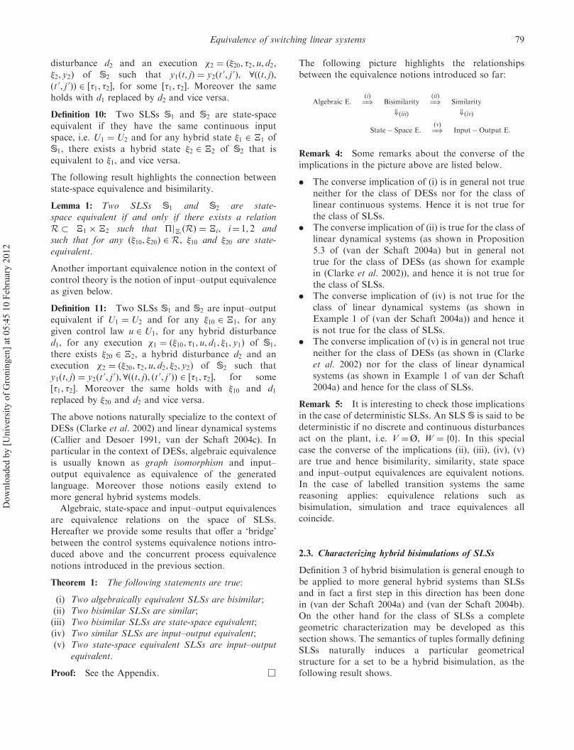
Theorem 1: The following statements are true:

(i) Two algebraically equivalent SLSs are bisimilar;

(ii) Two bisimilar SLSs are similar;

(iii) Two bisimilar SLSs are state-space equivalent;

(iv) Two similar SLSs are input–output equivalent;

(v) Two state-space equivalent SLSs are input–output

equivalent.

Proof: See the Appendix. œ

The following picture highlights the relationships

between the equivalence notions introduced so far:

Algebraic E: ¼)ðiÞ

Bisimilarity

+ðiiiÞ

¼)ðiiÞ

Similarity

+ðivÞ

State ÿ Space E: ¼)ðvÞ

InputÿOutput E:

Remark 4: Some remarks about the converse of the

implications in the picture above are listed below.

. The converse implication of (i) is in general not true

neither for the class of DESs nor for the class of

linear continuous systems. Hence it is not true for

the class of SLSs.

. The converse implication of (ii) is true for the class of

linear dynamical systems (as shown in Proposition

5.3 of (van der Schaft 2004a) but in general not

true for the class of DESs (as shown for example

in (Clarke et al. 2002)), and hence it is not true for

the class of SLSs.

. The converse implication of (iv) is not true for the

class of linear dynamical systems (as shown in

Example 1 of (van der Schaft 2004a)) and hence it

is not true for the class of SLSs.

. The converse implication of (v) is in general not true

neither for the class of DESs (as shown in (Clarke

et al. 2002) nor for the class of linear dynamical

systems (as shown in Example 1 of van der Schaft

2004a) and hence for the class of SLSs.

Remark 5: It is interesting to check those implications

in the case of deterministic SLSs. An SLS S is said to be

deterministic if no discrete and continuous disturbances

act on the plant, i.e. V ¼Ø, W ¼ f0g. In this special

case the converse of the implications (ii), (iii), (iv), (v)

are true and hence bisimilarity, similarity, state space

and input–output equivalences are equivalent notions.

In the case of labelled transition systems the same

reasoning applies: equivalence relations such as

bisimulation, simulation and trace equivalences all

coincide.

2.3. Characterizing hybrid bisimulations of SLSs

Definition 3 of hybrid bisimulation is general enough to

be applied to more general hybrid systems than SLSs

and in fact a first step in this direction has been done

in (van der Schaft 2004a) and (van der Schaft 2004b).

On the other hand for the class of SLSs a complete

geometric characterization may be developed as this

section shows. The semantics of tuples formally defining

SLSs naturally induces a particular geometrical

structure for a set to be a hybrid bisimulation, as the

following result shows.


Dow

nlo

aded

by [

Univ

ersi

ty o

f G

ronin

gen

] at

05:4

5 1

0 F

ebru

ary 2

012

Proposition 1: If R is a hybrid bisimulation between

two SLSs S1 and S2, there exists QR � Q1 �Q2 and

for any ðq1, q2Þ 2 QR suitable sets Rðq1, q2Þ � X1ðq1Þ �

X2ðq2Þ such that

q1, x1ð Þ, q2, x2ð Þð Þ 2 R()ðq1, q2Þ 2 QR and

ðx1, x2Þ 2 Rðq1, q2Þ:

Proof: The proof follows directly from the definition

of R being a subset of �1 ��2, and by the definition

of the hybrid spaces �1 and �2. œ

By the result above, any hybrid bisimulation R between

two SLSs S1 and S2 can be represented as

R ¼ ðq1, x1Þ, ðq2, x2Þð Þ 2 �1 ��2 j ðq1, q2Þ 2 QR,�

x1, x2Þ 2 Rðq1, q2Þð

: ð2Þ

Moreover the linearity in the continuous dynamics and

in the continuous variables spaces, leads to a particular

structure for the set Rðq1, q2Þ for any fixed pair

ðq1, q2Þ 2 QR. More precisely we now show that if R

is a hybrid bisimulation between two SLSs S1 and

S2, then the linear closure LðRÞ of R is a hybrid

bisimulation between S1 and S2.

More formally, given a hybrid bisimulation R as

in (2), between two SLSs S1 and S2, define the linear

closure LðRÞ of R as

LðRÞ ¼ ððq1, x1Þ, ðq2, x2ÞÞ 2 �1 ��2 j ðq1, q2Þ 2 QR,�

x1, x2Þ 2 LðRðq1, q2ÞÞð

,

where for any ðq1, q2Þ 2 QR, LðRðq1, q2ÞÞ is the linear

closure (Kelley and Namioka 1963) of Rðq1, q2Þ, i.e.

LðRðq1, q2ÞÞ ¼ �a � ðxa1, xa2Þ þ �b � ðxb1, x

b2Þ, 8�a,

�

�b 2 R, 8ðxa1, xa2Þ, ðx

b1, x

b2Þ 2 Rðq1, q2Þ

:

By definition of LðRÞ, R � LðRÞ; moreover the

following result holds.

Proposition 2: If R is a hybrid bisimulation between

two SLSs S1 and S2, then LðRÞ is a hybrid bisimulation

between S1 and S2.


By Propositions 1 and 2, from now on, any hybrid

bisimulation R between two SLSs S1 and S2 can be

represented by (2) where Rðq1, q2Þ is implicitly assumed

to be a linear subspace of X1ðq1Þ � X2ðq2Þ for any

ðq1, q2Þ 2 QR.

The following result gives an algebraic characteri-

zation of hybrid bisimulations for SLSs.

Theorem 2: Given two SLSs S1 and S2, a set R of

the form (2) is a hybrid bisimulation between S1 and S2

if and only if for any ðq1, q2Þ 2 QR the following property

holds:

8q 01 2 succðq1Þ, 9q

02 2 succðq2Þ [ fq2g : ðq

01, q

02Þ 2 QR and

(i) 1ðq1Þ ¼ 2ðq2Þ and Rðq1, q2Þ is a bisimulation

relation between �1ðq1Þ and �2ðq2Þ;

(ii) diagðM1ðe1Þ, �MM2ÞRðq1, q2Þ � Rðq 01, q

02Þ, where e1 2

E1 takes q1 into q 01 and e2 2 E2 takes q2 into q 0

2,

and �MM2 ¼ M2ðe2Þ if q02 6¼ q2, �MM2 ¼ I if q 0

2 ¼ q2;

and vice versa, 8q 02 2 succðq2Þ, 9q

01 2 succðq1Þ [ fq1g:

ðq 01, q

02Þ 2 QR and conditions (i) and (ii) are satisfied.

Proof: (Sufficiency.) Theorem 2 (i) ensures that for any

�10, �20ð Þ 2 R and any input function u1 ¼ u2 for any

hybrid disturbance d1 and for any execution �1 ¼

ð�10, �1, u1, d1, �1, y1Þ of S1, there exists a hybrid distur-

bance d2 and an execution �2 ¼ ð�20, �2, u2, d2, �2, y2Þ of

S2, such that Definition 3 (i) and (ii) are satisfied for

any ðt, 0Þ 2 ½�1�. Finally Theorem 2 (ii) ensures that

once the switching has occurred in S1 from some

ðq1, x1Þ to some ðq 01, x

01Þ and in S2 from some ðq2, x2Þ

to some ðq 02, x

02Þ the pair of continuous states

ðx 01, x

02Þ 2 Rðq 0

1, q02Þ. Hence by induction the result

follows.

(Necessity.) Suppose that R is a hybrid bisimulation

of the form (2) between S1 and S2. Necessity of

Theorem 2 (i) is obvious and can be proved by

contradiction. As far for the necessity of Theorem 2

(ii), for any ððq10, x10Þ, ðq20, x20ÞÞ 2 R, for any u1 ¼ u2for any hybrid disturbance d1, consider �1 ¼ fI0, I1g,

where I0 ¼ ft0g ¼ ft 00g and any execution �1 ¼

ð�10, �1, u1, d1, �1, y1Þ of S1: since R is a hybrid bisimula-

tion between S1 and S2, there exists a hybrid distur-

bance d2 and an execution �2 ¼ ð�20, �2, u2, d2, �2, y2Þ of

S2 such that Definition 3 (i) is satisfied 8ððt, jÞ, ðt 0, j 0ÞÞ 2

½�1, �2�, for some ½�1, �2�. In particular by writing

Definition 3 (i) in t ¼ t1, we have

ðM1ðe1Þx10, �MM2x20Þ 2 Rðq 01, q

02Þ: ð3Þ

Since condition (3) is true for any ðx10, x20Þ 2 Rðq10, q20Þ,

then Theorem 2 (ii) is satisfied for any fixed ðq10, q20Þ 2

QR. By repeating the same proof replacing q10 with q20and vice versa, Theorem 2 (ii) is satisfied. œ

Remark 6: Note that in the result above we do not

assume that R ¼ LðRÞ and hence Theorem 2 holds

also for hybrid bisimulations R for which R 6¼ LðRÞ.

Remark 7: Conditions outlined in Theorem 2 are

sufficient for characterizing hybrid bisimulations for

more general hybrid systems whose discrete transitions

depend on the continuous state x.

80 G. Pola et al.

Dow

nlo

aded

by [

Univ

ersi

ty o

f G

ronin

gen

] at

05:4

5 1

0 F

ebru

ary 2

012

By the result above, we may suppose w.l.o.g. that any

hybrid bisimulation satisfies conditions of Theorem 2.

Moreover a direct consequence of Theorem 2 is given

in the following.

Corollary 1: Two SLSs are bisimilar if and only if

there exists a set R � �1 ��2 of the form (2) satisfying

conditions of Theorem 2 and such that �j�iðRÞ ¼ �i,

i ¼ 1, 2.

In the next section we will show how to check the

conditions of the above result in a finite number of

steps and hence how to check bisimilarity of a pair of

SLSs.

If S1 and S2 are bisimilar with hybrid bisimulation R,

the dynamical systems �ðq1Þ and �ðq2Þ associated with

any pair ðq1, q2Þ 2 QR are not necessarily bisimilar as

the following example shows.

Example 1: Let us consider a pair of SLS S1 and S2

whose DESs DS1¼ D1 and DS2

¼ D2 are depicted in

figure 1 and where

M1ðq, v, q0Þ ¼

½I 0� if q ¼ q2, q 0 ¼ q3,

½IT 0T�T if q ¼ q3, q 0 ¼ q2,

I otherwise,

8

>

<

>

:

and M2ðeÞ ¼ I for any e 2 E2. Suppose that �1ðq1Þ ¼

�1ðq2Þ ¼ �2ðq4Þ ¼ �2ðq5Þ and Aðq4Þ ¼ diagfAðq3Þ,Ag,

Bðq4Þ ¼ ½Bðq3ÞT BT�T, Cðq3Þ ¼ ½Cðq1Þ C�, for some

matrices A, B and C of appropriate dimensions.

Consider a set R of the form (2), where

QR ¼ ðq1, q4Þ, ðq2, q5Þ, ðq3, q4Þ�

,

Rðq1, q4Þ ¼ ðx1, x4Þ : x1 ¼ x4�

,

Rðq2, q5Þ ¼ ðx2, x5Þ : x2 ¼ x5�

,

Rðq3, q4Þ ¼ ðx3, x4Þ : ðx3, 0Þ ¼ x4�

:

It is simple to check that R is a hybrid bisimulation

between S1 and S2 and �j�iðRÞ ¼ �i, i¼ 1, 2, thus S1

and S2 are bisimilar. However �2ðq4Þ and �1ðq3Þ are

not bisimilar.

On the other hand the following result holds.

Proposition 3: Consider two bisimilar SLSs S1 and S2

and a hybrid bisimulation R between S1 and S2 such

that �j�iðRÞ ¼ �i, i ¼ 1, 2. For any q1 2 Q1, there

exists q2 2 Q2 such that �1ðq1Þ � �2ðq2Þ and ðq1, q2Þ 2

QR and vice versa.

Proof: The proof follows directly from Definitions 3

and 4. œ

When formalizing hybrid bisimulations in Definition 3,

no restrictions were posed on hybrid time bases �1 and

�2 of executions �1 and �2 while in the definition of

structural hybrid bisimulation proposed in (van der

Schaft 2004c), �1 ¼ �2 was required. We now show

that by associating to any SLS S a suitable SLS S’

bisimilar to S, there is no loss of generality into setting

�1 ¼ �2, in Definition 3.

More precisely given an SLS S ¼ ð�,U,D,Y,

�, ,E,M Þ, define the SLS

S’

:¼ ð�,U,D,Y,�, ,E’,M’Þ,

where E’ :¼ E [ E 0 being E 0 :¼ fðq, v, qÞ, 8q 2 Q, for

some v 2 Vg and M’ðeÞ ¼ MðeÞ, if e 2 E, M’ðeÞ ¼ I,

if e 2 E 0. Then the following holds.

Proposition 4: Given two SLSs S1 and S2,

. S1 and S’1 are bisimilar;

. R is a hybrid bisimulation between S1 and S2

if and only if R is a hybrid bisimulation between S’1

and S2;

. R is a hybrid bisimulation between S1 and S2 if and

only if R is a hybrid bisimulation between S’1 and

S’2 and in this last case R satisfies Definition 3 with

�1 ¼ �2.

Remark 8: By considering S’1 and S

’2 , instead of S1

and S2, we implicitly force a time synchronization in

the events driving the discrete transitions in the time

evolution of each of the SLSs S’1 and S

’2 .

We conclude this section by defining the sum of hybrid

bisimulations between SLSs. Given two hybrid bisimu-

lations Ra and Rb between two SLSs S1 and S2,

Rab:¼ Ra þRb is called the sum of Ra and Rb if

Rab:¼ ðq1, x1Þ, ðq2, x2Þð Þ 2 �1 ��2jðq1, q2Þ

�

2 QRab , ðx1, x2Þ 2 Rabðq1, q2Þ

,

where QRab :¼ QRa [QRb and

Rabðq1, q2Þ

:¼

Raðq1, q2Þ þRbðq1, q2Þ, if ðq1, q2Þ 2 QRa \QRb ;

Raðq1, q2Þ, if ðq1, q2Þ 2 QRanQRb ;

Rbðq1, q2Þ, if ðq1, q2Þ 2 QRbnQRa :

8

>

<

>

:

Figure 1. DES D1 in the left and DES D2 in the right.


Dow

nlo

aded

by [

Univ

ersi

ty o

f G

ronin

gen

] at

05:4

5 1

0 F

ebru

ary 2

012

Proposition 5: Let Ra and Rb be hybrid bisimulations

between bisimilar SLSs S1 and S2. Then Ra þRb is a

hybrid bisimulation between S1 and S2.

Proof: By applying Theorem 2 to Ra þRb the state-

ment holds. œ

Remark 9: The results presented in this section are

developed in the context of continuous-time switching

linear systems. However the results of this section

still hold when characterizing hybrid bisimulations for

discrete-time switching linear systems.

3. Maximal hybrid bisimulation

In this section we characterize the properties and

we propose a procedure for the computation of the

maximal hybrid bisimulation.

The maximal hybrid bisimulation between (bisimilar)

SLSs S1 and S2 is a hybrid bisimulation R� between S1

and S2 such that, for all hybrid bisimulationsR between

S1 and S2, R � R�.

The following result summarizes some properties of the

maximal hybrid bisimulation.

Theorem 3: Given two SLSs S1 and S2 and the

maximal hybrid bisimulation R� between S1 and S2, the

following property hold:

(i) �j�iðR�Þ ¼ �i, i¼ 1, 2, if and only if S1 and S2 are

bisimilar.

Moreover if S1 and S2 are bisimilar then:

(ii) R� exists and is unique;

(iii) R� þR ¼ R�, for any hybrid bisimulation R

between S1 and S2;

(iv) R� ¼ LðR�Þ:


Hereafter we propose a procedure for the compu-

tation of R�. As in the case of linear dynamical

systems, the proposed procedure is very close to

procedures for the computation of the maximal safe

set for SLSs: its main ingredient is the one devel-

oped in (De Santis et al. 2004a) which computes

inner approximations of the maximal safe set for

the class of discrete-time switching linear systems

constrained to compact sets in the continuous state

and input.

The key idea is to first compute the maximal bisim-

ulation Q� of the discrete layers associated with the

pair of SLSs under consideration and then, to compute

the maximal hybrid bisimulation R� on the basis of Q�.

The computation of Q� may be performed by

using standard algorithms as for example the one in

(Clarke et al. 2002) which converges in a finite number

of steps to the maximal bisimulation relation for

DESs. Note that QR� � Q�, since in the computation

of Q� informations coming from the continuous

dynamics have not been considered.

The computation of R� may be done by combining

Algorithm 2 of (van der Schaft 2004a), which com-

putes the maximal bisimulation relation for linear

dynamical systems, with Procedure Switching of De

Santis et al. (2004) for the computation of maximal

safe sets for switching systems. Computing R�

requires the analysis of the topological properties of

DESs DS1and DS2

associated to SLSs S1 and S2.

For this purpose, it is useful to define the DES D�,

naturally induced by the bisimulation relation Q�.

More formally, let D� ¼ ðQ�,P�,V�,E�, �Þ be a DES

where:

. P� ¼ P1[ P2,

. V� ¼ V1 � V2,

. E� ¼ fððq1, q2Þ, ðv1, v2Þ, ðq01, q

02ÞÞ : ðq1, v1, q

01Þ 2

E1, ðq2, v2, q02Þ 2 E2, 1ðq1Þ ¼ 2ðq2Þ, 1ðq

01Þ ¼ 2ðq

02Þg,

. �ðq1, q2Þ ¼ 1ðq1Þ ¼ 2ðq2Þ, 8ðq1, q2Þ 2 Q�.

Proposition 6: Given two bisimilar SLSs S1 and S2,

D� is well defined.

The computation of the maximal hybrid bisimulation

R� exploits the topological properties of D�.

Before explaining the basic steps of the proposed

procedure for the computation of R�, we need to

recall well known facts about DESs (Hopcroft and

Ullman 1979).

A Strongly Connected Component (SCC) of D� is

the maximal set of mutually reachable states. We

denote by F, the set of all SCCs associated to D�.

SCCs determine a Directed Acyclic Graph (DAG).

Moreover F0 � F denotes the set of all SCCs not

reached by any SCCs, Fi � F denotes the set of all

SCCs, reached in one step by a SCC in Fiÿ1 and so

on. Let nF be the maximal integer i for which Fi is

nonempty. Notice that the intersection Fi \ Fj with

i 6¼ j may be non-empty. Any SCC in F0 (resp. in

FnF ) is called a root (resp. a leaf ) of the DAG asso-

ciated to D�. For any F 2 F, we denote by

QF � Q1 �Q2, the set of extended discrete states

belonging to F. Moreover for any extended discrete

state ðq1, q2Þ 2 QF for some F, succðq1, q2Þ denotes

the set of all extended discrete states that are succes-

sor of ðq1, q2Þ in F. Sets QF, 8F 2 F are a partition

of Q�. For any F of D�, the set succ(F) is composed

by those SCCs, reached by F in one step and SiðF Þ,

i¼ 1, 2 denote the pair of bisimilar SLSs naturally

induced by the DES D� and by continuous dynamics

associated to its extended discrete states.

GðFþ,FÿÞ � QFþ denotes the set of extended discrete

states of Fþ, reachable in one step by an

82 G. Pola et al.

Dow

nlo

aded

by [

Univ

ersi

ty o

f G

ronin

gen

] at

05:4

5 1

0 F

ebru

ary 2

012

extended discrete state in Fÿ. Moreover My denotes

the Moore–Penrose pseudo-inverse of a given

matrix M and Bisimð�1ðq1Þ,�2ðq2Þ, InitÞ denotes the

maximal linear bisimulation between �1 and �2

constrained to a subspace Init (see (van der Schaft

2004c) for an algorithmic procedure computing

Bisimð�1ðq1Þ,�2ðq2Þ, Init) in a finite number of

steps).

The computation of R� is based on Theorem 2 and is

carried out using a two step procedure:

. At the lower-level, we give a procedure for the

computation of the maximal hybrid bisimulation

between bisimilar SLSs S1ðF Þ and S2ðF Þ naturally

induced by a SCC F, constrained to a given subspace

InitðF Þ.

. At the higher-level, the computation of R� is

proposed and based on the lower-level procedure.

We start by describing how to compute the maximal

hybrid bisimulation BisimSCCðInitðF Þ,F Þ between

SLSs S1ðF Þ and S2ðF Þ induced by the SCC F of D�

and constrained in the hybrid subspace:

InitðF Þ ¼S

ðq1, q2Þ2QFðq1, q2Þ�

� InitFðq1, q2Þ:

We will define an appropriate recursion that, by exploit-

ing topological structure of F, computes a sequence of

sets KðiÞ, i ¼ 0, 1, . . . , converging to the maximal

hybrid bisimulation between S1ðF Þ and S2ðF Þ.

At first we set i ¼ 0 and the initial maximal hybrid

bisimulation Kð0Þ between S1ðF Þ and S2ðF Þ as

Kð0Þ :¼S


� Zððq1, q2Þ, 0Þ,

where Zððq1, q2Þ, 0Þ :¼ InitFðq1, q2Þ for any ðq1, q2Þ 2 QF.

For any ðq1, q2Þ 2 QF, we first update the con-

straining subspace Z0 where Bisimð�1ðq1Þ,�2ðq2Þ,Z0Þ

lies: for any ðq 01, q

02Þ 2 succðq1, q2Þ, by Theorem 2

(ii), Bisimð�1ðq1Þ,�2ðq2Þ,Z0Þ has to belong to

Myðe1, e2ÞZððq01, q

02Þ, 0Þ, where e1 and e2 connect discrete

states ðq1, q2Þ to ðq 01, q

02Þ. Compute

Z0 :¼T

ðq01, q0

2Þ2succðq1, q2Þ

Myðe1, e2ÞZððq01, q

02Þ, 0Þ: ð4Þ

Then it is possible to compute Zððq1, q2Þ, 0Þ :¼

Bisimð�1ðq1Þ,�2ðq2Þ,Z0Þ between �1ðq1Þ and �2ðq2Þ.

Finally we update Kð0Þ :¼ [ðq1, q2Þ2QFfðq1, q2Þg�

Zððq1, q2Þ, 0Þ and i :¼ iþ 1. By iterating this step

again the maximal hybrid bisimulation between

S1ðF Þ and S2ðF Þ corresponds to a fixed point

KðiÞ ¼ Kðiÿ 1Þ, for some i 2 N, of the recursion above.

The proposed procedure is formalized in the following

Function.

Function 1: RðF Þ :¼ BisimSCCðInitðF Þ,F Þ

set i :¼ 0

8ðq1,q2Þ 2QF

setZððq1,q2Þ, iÞ :¼ InitFðq1,q2Þ

setKðiÞ :¼S

ðq1,q2Þ2QFðq1,q2Þ�

�Zððq1,q2Þ, iÞ

whileKðiÞ 6¼Kðiÿ1Þ repeat

for any ðq1,q2Þ 2QF do

computeZ0 :¼T

ðq 01,q 0

2Þ2succðq1,q2Þ

Myðe1,e2ÞZððq01,q

02Þ, iÞ

where ek ¼ ðqk,vk,q0kÞ, vk 2Vk, k¼ 1,2

computeZððq1,q2Þ, iÞ ¼Bisimð�1ðq1Þ,�2ðq2Þ,Z0Þ

end do

setKðiÞ :¼S


�Zððq1,q2Þ, iÞ

set i :¼ iþ1

end while

returnRðF Þ :¼KðiÞ

end Function

We now provide the high-level algorithm. The

computation of the maximal hybrid bisimulation starts

from the leaves F 2 FnF and going backwards, ends to

the roots F 2 F0 of the DAG associated to D�. For any

F 2 F, Init(F) represents the constraining subspace

where the maximal hybrid bisimulation has to be

computed. Firstly we set

InitðF Þ :¼S


� InitFðq1, q2Þ, 8F 2 F:

Any F 2 FnF has no successors. The first step consists of

computing for any F 2 FnF , the maximal hybrid bisimu-

lation BisimSCCðInitðF Þ,FÞ associated to SLSs S1ðF Þ

and S2ðF Þ, induced by F. Then we need to update the

constraining subspace InitðFÿÞ of SCCs Fÿ 2

succÿ1ðFnF Þ: consider all SCCs Fþ 2 succðFÿÞ and all

extended discrete states ðq1, q2Þ 2 QFÿ that reach in one

step the extended discrete states ðq 01, q

02Þ 2 GðFþ,FÿÞ �

QFþ of Fþ. By Theorem 2 (ii), for any fixed Fþ 2

succðFÿÞ and for any fixed ðq 01, q

02Þ 2 GðFþ,FÿÞ, the set

Bisimððq1, q2Þ,Z0Þ has to belong to

�ðq 01, q

02Þ :¼ Myðe1, e2ÞBisimððq

01, q

02Þ, InitðF

þÞÞ, ð5Þ

where e1 and e2 connect ðq1, q2Þ 2 QFÿ to ðq 01, q

02Þ 2 QFþ .

By considering all extended discrete states ðq 01, q

02Þ 2

GðFþ,FÿÞ and all SCCs Fþ 2 succðFÿÞ, the maximal

hybrid bisimulation between S1ðFÿÞ and S2ðF

ÿÞ, has

to belong to

InitðFÿÞ :¼ InitðFÿÞT

I0ðFÿÞ


Dow

nlo

aded

by [

Univ

ersi

ty o

f G

ronin

gen

] at

05:4

5 1

0 F

ebru

ary 2

012

where

I0ðFÿÞ :¼T

Fþ2succðFÿÞ

T

ðq 01, q 0

2Þ2GðFþ,FÿÞ�ðq

01, q

02Þ

� �

:

Finally it is possible to go backwards and consider the

SCCs of FnFÿ1 and so on. This procedure ends when

all SCCs are visited. The resulting set R̂R can be thought

of as being of the form (2); moreover R̂R as returned by

the procedure may contain some empty sets. For this

reason define

CleanðR̂RÞ ¼ ððq1,x1Þ, ðq2, x2ÞÞ 2 R̂R : R̂Rðq1, q2Þ 6¼ Øn o

,

and finally set R̂R :¼ CleanðR̂RÞ. The proposed procedure

is formalized in the following algorithm.

Algorithm 1: MAXIMAL HYBRID BISIMULATION

set i :¼ nF, R̂R :¼Ø

8F2 F

set InitðF Þ :¼S


� InitFðq1,q2Þ

while i> 0 repeat

8F2 Fi

compute RðF Þ :¼ BisimSCCðInitðF Þ,F Þ

set R̂R :¼ R̂R[RðF Þ

8Fÿ 2 succÿ1ðF Þ

compute InitðFÿÞ :¼ InitðFÿÞT

I0ðFÿÞ, i :¼ iÿ1

end while

R̂R :¼ CleanðR̂RÞ

end Algorithm

Remark 10: Algorithm 1 makes use of geometric

linear control theory and therefore there are various effi-

cient tools in the literature for the effective computation

of the required sets.

Convergence properties of the procedure above is now

characterized.

Theorem 4: Algorithm 1 converges in a finite number of

steps to the maximal hybrid bisimulation R̂R ¼ R� or to the

empty set.

The result above is also important because it gives a

reformulation of Theorem 2 that is checkable in a finite

number of steps, as the following result shows.

Corollary 2: Two SLSs S1 and S2 are bisimilar if and

only if the returned set R̂R of Algorithm 1 is such that

�j�iðR̂RÞ ¼ �i, i¼ 1, 2.

We conclude this section by giving some results high-

lighting the computational complexity of the proposed

approach. The following results give an upper bound

on the number of steps for which the convergence of

Function BisimSCC and Algorithm 1 is ensured.

Proposition 7: Given a SCC F and an initial subspace

InitðF Þ, Function BisimSCCðInitðF Þ,FÞ converges in at

most @ðF Þ steps, where

@ðF Þ ¼ max dimX1ðq1Þ þ dimX2ðq2Þ, ðq1, q2Þ 2 QF

�

:

Proposition 8: Algorithm 1 converges in at most @

steps, where @ ¼P

F2F@ðF Þ.

The proof of the results above is based on the structure

of the sets involved being linear subspaces.

4. Reduction via hybrid bisimulation

Reduction via bisimulation is a well-known technique

to reduce the topological complexity of concurrent

processes (see for example (Hermanns 2002)). The

basic idea is to find a bisimulation between the process

and itself and then to factorize the state space of the

process under the equivalence relation induced by the

bisimulation. In this section, we extend results in

(Hermanns 2002) and (van der Schaft 2004a) to SLSs.

Therefore in the following we will consider an SLS S

and a copy of itself and we show how to perform a

hybrid state space reduction of S. The following obvious

facts hold.

Lemma 2: Given an SLS S, the identity relation

Rid :¼ fð�1, �2Þ j �1 ¼ �2g is a hybrid bisimulation between

S and itself.

Lemma 3: Given an SLS S, for any hybrid bisimu-

lation R between S and itself, Rÿ1:¼ fð�2, �1Þ j ð�1,

�2Þg 2 R is a hybrid bisimulation between S and itself.

Every R � �� naturally induces a relation on � by

saying that �1, �2 2 � are related by R if and only if

�1, �2ð Þ 2 R. For performing the hybrid state space

reduction of a given SLS, we employ an equivalence

relation on the hybrid state space � in such a way that

all hybrid states belonging to the same equivalence

class of the equivalence relation are reduced to the

same hybrid state. The following result shows that any

hybrid bisimulation naturally induces an equivalence

relation on the hybrid state space.

Proposition 9: For any hybrid bisimulation R between

an SLS S and itself there exists a hybrid bisimulation

R 0 between S and itself that is also an equivalence

relation on the hybrid state space � of S.

84 G. Pola et al.

Dow

nlo

aded

by [

Univ

ersi

ty o

f G

ronin

gen

] at

05:4

5 1

0 F

ebru

ary 2

012

Proof: Denote by Q 0 the set of all ðq1, q3Þ 2 Q1 �ð

Q2ÞnQR such that ðq1, q2Þ, ðq2, q3Þ 2 QR for some

q2 2 QR and set

R00 ¼ RS S

q1, q3ð Þ2Q 0f q1, q3ð Þg � R00 q1, q3ð Þ� �

,

where R00 q1,q3ð Þ ¼ fðx1,x3Þ 2 Xðq1Þ �Xðq3Þ j9x2 2 Xðq2Þ:

ðx1, x2Þ 2 R q1, q2ð Þ, ðx2, x3Þ 2 R q2, q3ð Þg is a linear bisim-

ulation between � q1ð Þ and � q3ð Þ. Set

R 0 ¼ R00 þ R00ð Þÿ1

þRid:

By construction R 0 is an equivalence relation on the

hybrid state space � of S. We now show that R00 is a

hybrid bisimulation between S and itself, and then by

Proposition 5, that R 0 is a hybrid bisimulation between

S and itself. For any ðq1, q2Þ 2 QR Theorem 2 (i) and

(ii) are satisfied. For any ðq1, q2Þ 2 Q 0, there exists

q3 2 Q such that ðq1, q2Þ, ðq2, q3Þ 2 QR. Then by defini-

tion, for any q 01 2 succðq1Þ, there exists q 0

2 2 succðq2Þ,

and for any q 02 2 succðq2Þ, there exists q 0

3 2 succðq3Þ

such that ðq 01, q

02Þ, ðq

02, q

03Þ 2 QR and hence ðq 0

1, q03Þ 2 QR.

Moreover ðq1Þ ¼ ðq2Þ ¼ ðq3Þ and R00 q1, q3ð Þ is a

bisimulation between �ðq1Þ and �ðq3Þ and therefore

Theorem 2 (i) is satisfied. For any ðx1, x3Þ 2 Rðq1, q3Þ

there exists x2 2 Xðq2Þ such that ðx1, x2Þ 2 Rðq1, q2Þ,

ðx2, x3Þ 2 Rðq2, q3Þ and ðM1ðe1Þx1,M2ðe2Þx2Þ 2 Rðq 01,

q 02Þ, ðM2ðe2Þx2,M3ðe3Þx3Þ 2 Rðq 0

2, q03Þ, with appropriate

discrete transitions ei, i ¼ 1, 2, 3, and therefore

ðM1ðe1Þx1,M3ðe3Þx3Þ 2 Rðq 01, q

03Þ, i.e. Theorem 2 (ii) is

satisfied. By repeating the same proof replacing the

role of q1 by q2, the statement follows. œ

Remark 11: R 0 as constructed in the proof above can

be seen as the closure of R with respect to the properties

of reflexivity, symmetry and transitivity.

Remark 12: Given a hybrid bisimulation R, the

hybrid bisimulation R 0, constructed in the proof of

Proposition 9, is such that R � R 0, and therefore it is

easy to see that the maximal hybrid bisimulation R�

between S and itself is also an equivalence relation.

By the result above we may assume w.l.o.g. that

the hybrid bisimulations under consideration are

equivalence relations on the hybrid state space � of S.

Given a hybrid bisimulation and equivalence relation

R, we now show how to perform a hybrid state space

reduction and how to define the reduced SLS bisimilar

to S.

Denote by i, the equivalence class induced by QR

such that qj, qk 2 i if and only if ðqj, qkÞ 2 QR. For

any i choose the set of representatives �i such that

. for any q 2 i there exists q�i 2 �i such that

�jXðqÞ Rðq, q�i Þÿ �

¼ XðqÞ,

. for any q, q 0 2 �i , q 6¼ q 0,�jXðq 0Þ Rðq, q 0Þð Þ 6¼ Xðq 0Þ.

The existence of �i is guaranteed by Proposition 3.

Denote by QR the set of all canonical represen-

tatives of the sequence i, i ¼ 1, 2, . . . , i.e. QR ¼S

i�i . For any q 2 QR define EðqÞ :¼ fq 0 2 Q:

ðq, q 0Þ 2 QRg, �RRðqÞ :¼ fx1 ÿ x2 j ðx1, x2Þ 2 Rðq, qÞg and

finally

�RR :¼S

q2QREðqÞ � �RRðqÞ:

The hybrid state space � of the SLS S under considera-

tion may be now factorized by �RR. We write �=R to

denote the reduced hybrid state space of S, naturally

induced by �RR, i.e.

�=R ¼S

q2QR q�

� XðqÞ= �RRðqÞ:

Let �RQ: Q ! QR be the canonical projection map

associating to each element of Q its unique canonical

representative in QR, and for any q 2 QR let �Rq :

XðqÞ ! XðqÞ=RðqÞ be the canonical projection. Define

the reduced SLS:

SR ¼ ð�R,U,D,Y,�R, R,ER,MRÞ,

where

. XRðqÞ ¼ XðqÞ= �RRðqÞ and dimRðqÞ ¼ dimðXRðqÞÞ,

8q 2 QR;

. For any q 2 QR, �RðqÞ is given by equations

�RðqÞ :

_xxðtÞ ¼ ARðqÞxðtÞ þ BRðqÞuðtÞ þ GRðqÞwðtÞ,

yðtÞ ¼ CRðqÞxðtÞ,

�

where the dynamical systems above are defined as in

van der Schaft (2004a); for the sake of completeness,

there exists a ‘feedback’ map K(q) such that

ðAðqÞ þ GðqÞKðqÞÞ �RRðqÞ � �RRðqÞ,

and thus AðqÞ þ GðqÞKðqÞ projects to a linear map

ARðqÞ: XRðqÞ ! XRðqÞ satisfying ARðqÞ�Rq ¼

�Rq AðqÞ þ GðqÞKðqÞð Þ; BRðqÞ ¼ �R

q BðqÞ; GRðqÞ ¼

�Rq GðqÞ; C

RðqÞ is such that CRðqÞ�Rq ¼ CðqÞ;

. R: QR!P such that RðqÞ ¼ ðqÞ, 8q 2 QR;

. e ¼ ðq 01, v, q

02Þ 2 ER if and only if there exist q1 2

Eÿ1ðq 01Þ and q2 2 Eÿ1ðq 0

2Þ such that ðq1, v, q2Þ 2 E;

. 8e ¼ ðq, v, q 0Þ 2 ER, MRðeÞ�Rq 0 ¼ �R

q MðeÞ.

The reduced SLS SR depends on the choice of the set

QR of canonical representatives of equivalence classes

induced by QR on Q. The following holds.


Dow

nlo

aded

by [

Univ

ersi

ty o

f G

ronin

gen

] at

05:4

5 1

0 F

ebru

ary 2

012

Proposition 10: Let R be a hybrid bisimulation and

equivalence relation between S and itself. Then for any

canonical representative QR,S and SR are bisimilar and

cardðQRÞ � cardðQÞ, dimðXðRQðqÞÞÞ � dimðXðqÞÞ, 8q 2Q:

Proof: For any QR define R 0 � ��= �RR such that

ððq, xÞ, ðq 0, x 0ÞÞ 2 R 0 if and only if �RQðqÞ ¼ q 0 and

�Rq ðxÞ ¼ x 0. It is easily seen that R 0 is a hybrid

bisimulation such that �j�ðR0Þ ¼ � and �j�=R

ðR 0Þ ¼

�=R. The second part of the statement is obvious by

construction. œ

Remark 13: The second part of the statement of

Proposition 10 formalizes the intuitive idea that SR is

in some way ‘smaller’ than S.

The following result is a direct consequence of

Proposition 10 and of the definition of reduced SLSs.

Corollary 3: LetR1 andR2 be hybrid bisimulations and

equivalence relations between S and itself such that

R2 � R1. Then,

cardðQR1 Þ � cardðQR2 Þ,

dimðXð�R1

QðqÞÞÞ � dimðXð�R2

QðqÞÞÞ, 8q 2 Q:

These results reveal a sort of monotony in the functions

cardðQRÞ and dimðXð�RQðqÞÞÞ, 8q 2 Q depending on R.

Moreover, in view of the result above one may think

to find the minimal bisimilar SLS of an SLS S, by

reducing S by means of R�. We now show that this

intuitive idea is true.

We formally refer to a minimal bisimilar SLS of a

given SLS S as an SLS S0 that is bisimilar to S, and

such that the cardinality of its discrete state space Q 0

and the dimensions of its continuous state space

X 0ðqÞ, q 2 Q 0 are minimal among all other SLSs that

are bisimilar to S. Denote by minðSÞ the class of

minimal bisimilar SLSs of S. From Corollary 3 and the

definition of maximal hybrid bisimulation we derive the

following result.

Corollary 4: Let R� be the maximal hybrid bisimula-

tion between S and itself, then SR�

2 minðSÞ:

Remark 14: It is worth to point out that, by the

procedures illustrated in x 3, the computation of SR�

can be done in a finite number of steps. This result is

also important because shows that the minimal bisimilar

SLS of a given SLS can be always computed, whereas

the same reasoning does not apply to the general case

of hybrid systems, as shown in (Alur et al. 2000).

We recall the following result that will be instrumental

in the subsequent developments.

Lemma 4 (van der Schaft 2004c): If �1 and �2 are

bisimilar linear dynamical systems, then any � 01 2

minð�1Þ and any � 02 2 minð�2Þ are algebraically

equivalent.

Since SR�

depends on the set QR�

of canonical represen-

tatives of Q, it is not unique. However, the following

result holds.

Proposition 11: The family ofSR�

parametrized by QR�

,

is composed of SLSs that are algebraically equivalent.


Finally, using the same arguments as in the proof above,

it is simple to derive a generalization of Lemma 4 to

SLSs:

Corollary 5: If S1 and S2 are bisimilar, then

any S01 2 minðS1Þ and S

02 2 minðS2Þ are algebraically

equivalent.

5. Simulation and abstraction

Aim of this section is to characterize the notion of

simulation as introduced in Definition 5 and to

introduce the notion of abstraction for the class of SLSs.

By specializing Theorem 2, the following result is

obtained.

Theorem 5: Given two SLSs S1 and S2, a set R of

the form (2) is a simulation of S1 by S2 if and only if

for any ðq1, q2Þ 2 QR the following property holds:

8q 01 2 succðq1Þ, 9q

02 2 succðq2Þ [ fq2g: ðq

01, q

02Þ 2 QR and

(i) 1ðq1Þ ¼ 2ðq2Þ and Rðq1, q2Þ is a simulation relation

of �1ðq1Þ by �2ðq2Þ;

(ii) diagðM1ðe1Þ, �MM2ÞRðq1, q2Þ � Rðq 01, q

02Þ, where e1 2

E1 takes q1 into q 01 and e2 2 E2 takes q2 into q 0

2,

and �MM2 ¼ M2ðe2Þ if q02 6¼ q2, �MM2 ¼ I if q 0

2 ¼ q2;

Remark 15: On the basis of the above result and by

specializing the proposed procedure for the computation

of the maximal hybrid bisimulation given in x 3, it is

possible to give a procedure for the computation of

the maximal hybrid simulation of an SLS S1 by an

SLS S2. This is done by replacing the algorithms for

the computation of the maximal bisimulation of DESs

and of linear dynamical systems (see x 3) with the ones

in (Clarke et al. 2002) and (van der Schaft 2004a), com-

puting respectively the maximal simulation of a DES D1

by a DES D2, and the maximal simulation of a dynami-

cal system �1 by a dynamical system �2. The proposed

procedure converges to the maximal simulation of S1 by

S2 in a finite number of steps.

86 G. Pola et al.

Dow

nlo

aded

by [

Univ

ersi

ty o

f G

ronin

gen

] at

05:4

5 1

0 F

ebru

ary 2

012

By combining the results on reduction of SLSs given

in x 4 with the above results on hybrid simulations:

Proposition 12: Let S1 and S2 be two SLSs, such that

S2 is simulated by S1. Let R1 and R2 be respectively

hybrid bisimulations and equivalence relations, between

S1 and itself and S2 and itself. Then SR2

2 4SR1

1 .

Proof: SR2

2 4S2 4S1 4SR1

1 . œ

The notion of simulation is very close to the notion of

abstraction. Abstraction of concurrent processes and

dynamical systems has been studied in (Henzinger

1995), (Alur et al. 2000), (Tabuada et al. 2002) and

(Pappas 2003). The main idea is to ‘simplify’ the given

process under consideration in such a way that the

resulting process simulates the original one. In other

words, we may say that abstraction is related to

simulation in the same way as reduction is related

to bisimulation. Following (Pappas 2003) and (van

der Schaft 2004c) abstractions of SLSs are defined as

follows. Let S ¼ ð�,U,D,Y,�, ,E,MÞ be an SLS

where � ¼ [q2Qfqg � XðqÞ. Define a suitable set

�A ¼

S

q2QA q�

� XAðqÞ,

such that QA�Q and ðQAÞ ¼ ðQÞ and for any q 2 QA,

let XAðqÞ be a linear subspace of XðqÞ. Define a surjective

map M: � ! �A, such that

Mðq, xÞ ¼ ðMQðqÞ,MqxÞ, 8ðq, xÞ 2 �,

where MQ: Q!QA and for any q 2 Q,Mqx is linear

in x. Suppose that for any q 2 Q, kerMq � kerCðqÞ.

The map M naturally induces the SLS

SA:¼ �

A,U,D,Y,�A, A,EA,MAÿ �

,

where

. For any q 2 QA, �AðqÞ is given by equations

_xxðtÞ ¼ AAðqÞxðtÞ þ BAðqÞuðtÞ þ GAðqÞwðtÞ,

yðtÞ ¼ CAðqÞxðtÞ,

where AAðqÞ :¼ MqAðqÞMyq, BAðqÞ :¼ MqBðqÞ,

CAðqÞ :¼ CðqÞMyq, G

AðqÞ :¼ Mq½GðqÞ...AðqÞz1ðqÞ

.

.

.. . .

.

.

.

AðqÞzrðqÞðqÞ�, where z1ðqÞ, . . . , zrðqÞðqÞ span kerMq;

. Aðq 0Þ ¼ ðMÿ1Q ðqÞÞ for some q 2 Q;

. e ¼ ðq 01,w, q

02Þ 2 EA if and only if there exist q1 2

Mÿ1Q ðq 0

1Þ and q2 2 Mÿ1Q ðq 0

2Þ such that ðq1,w, q2Þ 2 E;

. MAðeÞ ¼ Mq0MðeÞMyq, for any ðq,w, q 0Þ 2 EA.

We think of SA as an abstraction of S.

Remark 6: It is easily seen that one can associate to

any hybrid system H whose discrete transitions depend

on the continuous state x, a suitable switching system

S, whose discrete transitions are caused by external

discrete disturbances, and which is an abstraction of H.

The following result holds.

Proposition 13: S4SA.

Proof: Define the following set R 0 � ��A such that

ððq, xÞ, ðq 0, x 0ÞÞ 2 R 0 if and only if MQðqÞ ¼ q 0 and

MqðxÞ ¼ x 0. It is easily seen that R 0 is a hybrid

simulation of S by SA such that �j�ðR

0Þ ¼ � and

�j�AðR 0Þ ¼ �A. œ

We conclude this section by establishing connections

between bisimulation-based reduction and simulation-

based abstraction.

Proposition 14: Given an SLS S and a hybrid

bisimulation R between S and itself, then SR is an

abstraction of S.

Proof: Set �A :¼ �=R. By definition ðQAÞ ¼ ðQÞ

and XAðqÞ is a linear subspace of XðqÞ for any q 2 QA.

Finally define MQ :¼ �RQ

and Mq :¼ �Rq , for any

q 2 Q. Since by definition for any q 2 Q,CRðqÞ�Rq ¼

CðqÞ, then for any x 2 ker�Rq , x 2 kerCðqÞ: thus,

ker�Rq � kerCðqÞ for any q 2 Q, and the statement

holds. œ

The converse of the previous statement obviously is not

true in general.

6. Connections with observability of SLSs

We outlined in x 2.2 that bisimilarity between SLSs

implies their input–output equivalence. This means

that any SLS S has the nice property that any reduced

SLS SR of S is input–output equivalent to S. In this

section, we will analyze the preservation of the structural

property of observability under bisimulation-based

reduction and simulation-based abstraction.

The class of SLSs that we consider in this context are

characterized by deterministic continuous dynamics,

i.e. W ¼ 0f g, unconstrained input and output functions,

i.e. U ¼ Rm and H ¼ R

s,m, s 2 N, and a minimum dwell

time �m > 0 , (Morse 1996) such that for any hybrid time

basis �, 8Ij 2 �, t 0j ÿ tj � �m.

We recall here the definition of observability proposed

in (De Santis et al. 2003)

Definition 12: An SLS S ¼ ð�,Rm,V� f0g,P� Rs,

�, ,E,MÞ is observable if there exist a function

’: CðRþ0 �N,RsÞ � CðN,PÞ�C0ðRþ

0 ,U Þ ! �,


Dow

nlo

aded

by [

Univ

ersi

ty o

f G

ronin

gen

] at

05:4

5 1

0 F

ebru

ary 2

012

an integer j � 0 and a real number � 2 0, �mð Þ such that

8�0 2 �, 8� 2 T , 8v 2 CðN,V Þ there exists an execution

� ¼ �0, �, u, d, �, yð Þ such that ’ðyj½ðt0, 0Þ, ðt, jÞ�, uj½t0, tÞÞ ¼

�ðt, j Þ, 8t 2 ðtj þ �, t 0j �, 8j ¼ j, jþ 1, . . . , cardð�Þ ÿ 1, where

yj ðt0, 0Þ, ðt, jÞ½ � is the restriction of the output y(t, j) to

½tj, tj�, 0 � j � j � j S is said to be unobservable if it is not

observable. A necessary and sufficient condition for

testing observability of SLSs is given in the following.

Theorem 6 (De Santis et al. 2003): An SLS

S ¼ ð�,Rm,V� f0g,P� Rs,�, ,E,MÞ is observable if

and only if

(i) �ðqiÞ is observable, 8qi 2 Q;

(ii) 8qi, qj 2 Q, qi 6¼ qj, one of the following conditions

hold:

– ðqiÞ 6¼ ðqjÞ,

– 9k 2N[ 0f g : CðqiÞAðqiÞkBðqiÞ 6¼ CðqjÞAðqjÞ

kBðqjÞ:

The problem that we address now is the preservation

of observability under bisimulation reduction. The

following result holds.

Proposition 15: If an SLS S is observable then

S 2 minðSÞ.

Proof: Let R be any hybrid bisimulation and equiva-

lence relation between S and itself. Since Theorem 6

(ii) holds, by Theorem 2, QR ¼ fðq, qÞ : q 2 Qg.

Moreover for any q 2 Q, since �ðqÞ is observable, by

Corollary 6.4 in (van der Schaft 2004c), Rðq, qÞ ¼

fðx, xÞ : x 2 XðqÞg. Therefore any hybrid bisimulation

and equivalence relation between S and itself coincides

with Rid and then S 2 minðSÞ. œ

The converse of the result above is proved in (van der

Schaft 2004c) for the class of linear dynamical systems.

However the following counterexample shows that it is

not true for the class of SLSs.

Example 2: Let us consider an SLS S3, whose DES

DS3¼ D3 is depicted in figure 2 and whose continuous

dynamics are such that �3ðq6Þ ¼ �3ðq7Þ ¼ �3ðq8Þ ¼

�3ðq9Þ and where M3ðeÞ ¼ I, for any e 2 E3. Suppose

that �3ðqiÞ are observable for any qi, i ¼ 6, . . . , 9.

S3 2 minðS3Þ and is unobservable since Theorem 6 (ii)

is not satisfied for q6, q7.

It is important to emphasize that unobservable SLSs

may give rise to reduced observable or unobservable

SLSs. This motivates the introduction of the following

unobservable SLSs classification.

Definition 13: An SLS S is said to be

. Non-properly unobservable if it is unobservable

and there exists a hybrid bisimulation R between

S and itself, such that the reduced SLS SR is

observable,

. Properly unobservable if it is unobservable and for

any hybrid bisimulation R between S and itself

the reduced SLS SR is unobservable.

Example 3: Let us consider an SLS S2, whose DES

DS2¼ D2 is depicted in figure 2 and whose continuous

dynamics are such that �2ðq3Þ ¼ �2ðq4Þ ¼ �2ðq5Þ and

observable and where M2ðeÞ ¼ I, for any e 2 E2. S2 is

unobservable since Theorem 6 (ii) is not satisfied for

q3, q5 It is simple to check that any minimal bisimilar

SLS S02 2 minðS2Þ of S2, whose DES is algebraically

equivalent to D1, with �QR� ðq3Þ ¼ �QR� ðq5Þ ¼ q2,

�QR� ðq4Þ ¼ q1, is observable. Then S2 is nonproperly

unobservable.

Example 4: Let us consider an SLS S3, whose

DES DS3¼ D3 is depicted in figure 2 and whose

continuous dynamics are such that �3ðq6Þ ¼ �3ðq7Þ ¼

�3ðq8Þ ¼ �3ðq9Þ and where M3ðeÞ ¼ I, for any e 2 E3.

Suppose that �3ðqiÞ are observable for any qi,

i ¼ 6, . . . , 9. S3 is unobservable since Theorem 6 (ii) is

not satisfied for q6, q7. Moreover it is simple to

check that S3 2 minðS3Þ. Since the only hybrid bisimu-

lation between S3 and itself is the identity relation

Rid, SRid

3 is unobservable and hence S3 is properly

unobservable.

Non-proper and proper unobservability can be charac-

terized as follows.

Proposition 16: An SLS S is non-properly unobservable

if and only if S is unobservable and any S0 2 minðSÞ is

observable.

Proof: Sufficiency holds by definition. For the

necessity part, suppose by contradiction that S is

observable or 9S 0 2 minðSÞ unobservable. If S is

Figure 2. DESs D1, D2, D3 and D4.

88 G. Pola et al.

Dow

nlo

aded

by [

Univ

ersi

ty o

f G

ronin

gen

] at

05:4

5 1

0 F

ebru

ary 2

012

observable a contradiction holds. Now suppose

9S 0 2 minðSÞ unobservable. If S0 is unobservable,

by Theorem 6 and Corollary 6.4 in (van der

Schaft 2004c), there exist q1, q2 2 QR�

, such that

R�

ðq1Þ ¼ R�

ðq2Þ and �R�

ðq1Þ � �R�

ðq2Þ. It is simple to

check by definition of S0, that any pair ðq 0

1, q02Þ 2

�ÿ1Q ðq1Þ ��ÿ1

Q ðq2Þ � Q�Q is such that for any hybrid

bisimulation and equivalence relation R between S

and itself, ðq 01, q

02Þ =2QR, and then the reduced SLS S

R

will have two discrete states �Qðq01Þ, �Qðq

02Þ 2 QR such

that Rð�Qðq01ÞÞ ¼ Rð�Qðq

02ÞÞ and �Rð�Qðq

01ÞÞ �

�Rð�Qðq02ÞÞ; then S

R is unobservable for any R, and

hence S is not nonproperly unobservable. œ

Proposition 17: An SLS S is properly unobservable if

and only if S is unobservable and any S0 2 minðSÞ is

unobservable.

The proof of the result above is an easy consequence of

Definition 13 and Proposition 16, and is therefore

omitted.

Remark 16: Conditions of Propositions 16 and

17 may be easily checked by constructing the

minimal bisimilar SLS of the given SLS S. As pointed

out in Remark 14, this construction reduces to the

computation of the maximal hybrid bisimulation

between the SLS S and itself, as formalized in

Corollary 4.

In view of the discussion above, reduction via hybrid

bisimulation is a good tool to extract the observable

dynamics of any non-properly unobservable SLS.

This result clearly links to the well known Kalman

decomposition of linear dynamical systems, that has

been recently extended to the class of SLSs (see (De

Santis et al. 2003, 2004b)). However if one wants to

extract the observable dynamics of a properly unobserv-

able SLS, reduction is not the right tool as shown by

Example 4. Therefore the key idea is to use abstraction

instead of reduction. The following result formalizes

that idea.

Proposition 18: For any properly unobservable SLS S,

there exists an abstraction SA of S which is observable

and which simulates S.

Proof: Define QA such that 6 9qi, qj 2 QA, qi 6¼ qj such

that ðqiÞ ¼ ðqjÞ and for any q 2 Q set Mq :¼ �R�

q

and �R�

q : XðqÞ ! XðqÞ=R�ðqÞ, R�ðqÞ being the maximal

linear bisimulation between �(q) and itself, for any

q 2 Q. Since, as shown in the proof of Proposition

14, kerMq � kerCðqÞ, the SLS SA is an abstraction

of S. By construction �AðqÞ is observable for any

q 2 Q (see van der Schaft (2004c)) and then SA

satisfies conditions of Theorem 6: therefore SA is

observable and finally by Proposition 13 the

statement holds. œ

The following example shows an application of

Proposition 18.

Example 5: Consider SLS S3 of Example 4. Define an

SLS S4, whose DES DS4¼ D4 is depicted in figure 2

and where �4ðq10Þ ¼ �4ðq11Þ ¼ �4ðq12Þ :¼ �3ðq6Þ and

M4ðeÞ ¼ I, for any e 2 E4. S4 is observable, is an

abstraction of S3 and simulates S3:

7. Some possible extensions

Aim of this section is to briefly discuss some possible

extensions of the proposed methodology for reducing

the complexity of the class of switching linear systems.

In fact the proposed results are easily extendable to

switching systems where the continuous dynamics are

governed by non-linear control systems or by linear

systems in pencil forms.

The key results to be generalized in these new

frameworks are:

. Theorem 2, characterizing the algebraic properties

for a set to be a hybrid bisimulation for the class

of switching systems under consideration,

. The procedures described in x 3 for computing the

maximal hybrid bisimulation,

. The definition of reduced switching systems as

formalized in x 4.

In the following we offer some remarks for generalizing

these key results in the case of switching non-linear

systems and of switching systems in pencil form.

We refer to a switching non-linear system, respectively

to a switching linear system in pencil form, as a tuple

ð�,U,D,Y,�, ,E,MÞ as in Definition 1 where � is

replaced by the following function that associates to

any discrete state q 2 Q, the non-linear dynamical

system

�ðqÞ :_xxðtÞ ¼ aðq, xðtÞÞ þ bðq, xðtÞÞuðtÞ þ gðq, xðtÞÞwðtÞ,

hðtÞ ¼ cðq, xðtÞÞ, t � 0;

�

að�, �Þ, bð�, �Þ, gð�, �Þ and cð�, �Þ being sufficiently smooth

vector fields, respectively by the following function

associating to any discrete state q 2 Q, the linear

dynamical system in pencil form

�ðqÞ:LðqÞ _xxðtÞ ¼ AðqÞxðtÞ,

wðtÞ ¼ HðqÞxðtÞ,

�

with Lð�Þ, Að�Þ and Hð�Þ being matrices of appropriate

dimensions. The notion of executions of switching

non-linear systems and switching linear systems in


Dow

nlo

aded

by [

Univ

ersi

ty o

f G

ronin

gen

] at

05:4

5 1

0 F

ebru

ary 2

012

pencil form can be easily generalized from Definition 2

and is therefore omitted.

It is worth to point out that Theorem 2 is still true

both for the class of switching non-linear systems and

for the class of switching linear systems in pencil form.

In particular note that Theorem 2 (i) implicitly requires

that Rðq1, q2Þ is a bisimulation relation between the pair

of dynamical systems �1ðq1Þ and �2ðq2Þ. An algebraic

characterization of bisimulations for non-linear

systems can be found in Proposition 7.9 of (van der

Schaft 2004c) and an algebraic characterization of

bisimulations for linear dynamical systems in pencil

form can found in Theorem 3.2. of (van der Schaft

2004b).

As far as for the computation of the maximal hybrid

bisimulation, it can be done by generalizing procedures

described in x 3, where the operator Bisimð�, �Þ should

be replaced by Algorithm 7.5 of (van der Schaft

2004c) in the case of switching non-linear systems, and

by Algorithm 3.3 of (van der Schaft 2004b), in the

case of switching linear systems in pencil forms.

Finally in view of the remarks above showing how

to compute the maximal hybrid bisimulation, the

reduced switching non-linear system and the reduced

switching linear system in pencil form may be defined

following the guidelines of x 4; we leave the details to

the reader.

8. Conclusions and outlook

In this paper we studied bisimulation for the class of

switching linear systems. The proposed definition is

mainly inspired by the classical notions given for

concurrent processes (Park (1981), Milner (1989),

Clarke et al. (2002), Hermanns (2002)) and by the

definitions introduced in (van der Schaft 2004a, b, c).

The definition considers the general case where the

switching mechanisms in the switching linear systems

may be asynchronous. Moreover the definition includes

more general frameworks of hybrid systems as for

example the case of discrete transitions depending on

the continuous state x.

A complete algebraic characterization of bisimulation

has been developed by combining tools from the theory

of concurrent processes (Clarke et al. (2002), Hermanns

(2002)) with those from control theory (De Santis et al.

(2004a), van der Schaft 2004a)). Moreover an algori-

thmic procedure converging to the maximal hybrid

bisimulation relation in a finite number of steps has

been developed: this procedure allows the computation

of the minimal bisimilar SLS of a given SLS and offers

some interesting links to the analysis of observability

of SLSs as given in (De Santis et al. 2003).

The proposed approach easily extends to the case of

discrete-time switching linear systems. Moreover, x 7

gives some guidelines for generalizing the results of

this paper to the case of switching non-linear systems

and switching systems in pencil form. The presented

results give also sufficient conditions for characterizing

hybrid bisimulations for more general hybrid systems

models with x-dependent discrete transitions. For

instance an SLS S can be easily constructed to mimic

the behaviour of a hybrid system H whose discrete

transitions are x-dependent in such a way that S is an

abstraction of H; therefore a preliminary sub-optimal

state space reduction of H can be pursued by reducing

S: this last approach is important also in view of the

results shown in (Alur et al. 2000) that proves the

non-decidability of bisimulation-based reduction for

general hybrid systems.

Following the guidelines of the proposed approach an

extension of the present results would be the study

of bisimulation theory for hybrid systems with

x-dependent discrete transitions.

Acknowledgement

The first author wishes to thank Mihaly Petreczky,

CWI, The Netherlands, for useful suggestions on reduc-

tion issue of Section 4. This work has been partially sup-

ported by the HYCON Network of Excellence, contract

number FP6-IST-511368.

Appendix: Technical proofs

Proof of Theorem 1: (Proof of (i)). With reference to

Definition 8, given two SLSs S1 and S2 let

R � �1 ��2 be such that ððq1, x1Þ, ðq2, x2ÞÞ 2 R if and

only if q2 ¼ TQðq1Þ and x2 ¼ Tq1ðx1Þ. By construction

R is a hybrid bisimulation between S1 and S2, such

that �j�iðRÞ ¼ �i, i¼ 1, 2.

(Proof of (ii)). Obvious by definition.

(Proof of (iii)). Since S1 and S2 are bisimilar there

exists a hybrid bisimulation R � �1 ��2 such that

�j�iðRÞ ¼ �i, i¼ 1, 2 and that therefore satisfies

conditions of Lemma 1.

(Proof of (iv)). For any given control law u 2 U1,

for any �10 2 �1, consider a hybrid state �20 2 �2 such

that ð�10, �20Þ 2 R for some hybrid simulation R of S1

by S2. By definition for any hybrid disturbance d1, for

any execution �1 ¼ ð�10, �1, u, d1, �1, y1Þ of S1, there

exists a hybrid disturbance d2 and an execution �2 ¼

ð�20, �2, u, d2, �2, y2Þ of S2 such that y1ðt, j Þ ¼ y2ðt0, j 0Þ,

8ððt, j Þ, ðt 0, j 0ÞÞ 2 ½�1, �2�, for some ½�1, �2�. Moreover the

90 G. Pola et al.

Dow

nlo

aded

by [

Univ

ersi

ty o

f G

ronin

gen

] at

05:4

5 1

0 F

ebru

ary 2

012

same holds with �10 and d1 replaced by �20 and d2 and

vice versa and hence the statement holds.

(Proof of (v)). For any given control law u 2 U1, for

any �10 2 �1, consider a state-equivalent hybrid state

�20 2 �2. By definition for any hybrid disturbance d1,

for any execution �1 ¼ ð�10, �1, u, d1, �1, y1Þ of S1, there

exists a hybrid disturbance d2 and an execution

�2 ¼ ð�20, �2, u, d2, �2, y2Þ of S2 such that y1ðt, j Þ ¼

y2ðt0, j 0Þ, 8ððt, j Þ, ðt 0, j 0ÞÞ 2 ½�1, �2�, for some ½�1, �2�.

Moreover the same holds with �10 and d1 replaced by

�20 and d2 and vice versa and hence the statement

holds. œ

Proof of Proposition 2: By construction, for any

ð�10, �20Þ 2 LðRÞ, where �10 ¼ ðq10, x10Þ and �20 ¼

ðq20, x20Þ, there exists �a, �b 2 R and ðxa10, xa20Þ,

ðxb10, xb20Þ 2 Rðq10, q20Þ such that ðx10, x20Þ ¼ �aðxa10,

xa20Þ þ �bðxb10, xb20Þ. Take any input function u1 ¼ u2 ¼ u

and any hybrid disturbance d1 ¼ ðv1,w1Þ. Choose some

ua1, ub1 2 C0ðRþ

0 ,U1Þ and some wa1,w

b1 2 C0ðRþ

0 ,W1Þ such

that

u1 ¼ �aua1 þ �bub1, w1 ¼ �awa1 þ �bwb

1:

For any execution �1 ¼ ððq10, x10Þ, �1, u1, ðv1,w1Þ, �1, y1Þ

of S1, there exists executions �a1 ¼ ððq10, x

a10Þ, �1, u

a1,

ðv1,wa1Þ, �

a1, y

a1Þ and �b

1 ¼ ððq10, xb10Þ, �1, u

b1, ðv1,w

b1Þ, �b1, y

b1Þ

of S1, such that

x1ðt, jÞ ¼ �axa1ðt, jÞ þ �bxb1ðt, jÞ,

h1ðt, jÞ ¼ �aha1ðt, jÞ þ �bhb1ðt, jÞ, 8ðt, jÞ 2 ½�1�,ð6Þ

where �1 ¼ ðq1, x1Þ, �a1 ¼ ðqa1, x

a1Þ, �b1 ¼ ðqb1, x

b1Þ, y1 ¼

ð p1, h1Þ, ya1 ¼ ð pa1, h

a1Þ, y

b1 ¼ ð pb1, h

b1Þ. Moreover, since

ðxa10, xa20Þ, ðx

b10, x

b20Þ 2 Rðq10, q20Þ, there exist hybrid

disturbances da2 ¼ ðv2,wa2Þ 2 D2 and db2 ¼ ðv2,w

b2Þ 2 D2

and executions �a2 ¼ ððq20, x

a20Þ, �2, u

a2, ðv2,w

a2Þ, �

a2, y

a2Þ

and�b2 ¼ ððq20, x

b20Þ, �2, u

b2, ðv2,w

b2Þ, �

b2, y

b2Þ of S2, such that

�a1ðt, jÞ, �a2ðt

0, j 0Þÿ �

2 R, ya1ðt, jÞ ¼ ya2ðt0, j 0Þ,

�b1ðt, jÞ, �b2ðt

0, j 0Þÿ �

2 R, yb1ðt, jÞ ¼ yb2ðt0, j 0Þ,

ð7Þ

8ððt, jÞ, ðt 0, j 0ÞÞ 2 ½�1, �2�, for some ½�1, �2�. By choosing a

hybrid disturbance d2 ¼ ðv2,w2Þ where w2 ¼ �awa2 þ

�bwb2, there exists an execution �2 ¼ ððq20, x20Þ, �2, u2,

ðv2,w2Þ, �2, y2Þ of S2 such that

x2ðt, jÞ ¼ �axa2ðt, jÞ þ �bxb2ðt, jÞ,

h2ðt, jÞ ¼ �aha2ðt, jÞ þ �bhb2ðt, jÞ, 8ðt, jÞ 2 ½�2�, ð8Þ

and hence by combining (6), (8) and (7),

ðx1ðt, jÞ, x2ðt0, j0ÞÞ ¼ �a � ðxa1ðt, jÞ, x

a2ðt

0, j0ÞÞ

þ �b � ðxb1ðt, jÞ, xb2ðt

0, j0ÞÞ

2 LðRðq1ð j Þ, q2ð j ÞÞÞ,

h1ðt, jÞ ¼ h2ðt0, j0Þ, 8ððt, jÞ, ðt0, j0ÞÞ 2 ½�1, �2�, for some ½�1, �2�:

Therefore �1ðt, jÞ, �2ðt0, j 0Þð Þ 2 LðRÞ and y1ðt, jÞ ¼

y2ðt0, j 0Þ, 8ððt, jÞ, ðt 0, j 0ÞÞ 2 ½�1, �2�, for some ½�1, �2�.

By repeating the same proof with d1 replaced by d2and vice versa the statement holds. œ

Proof of Theorem 3: We only have to prove Theorem

3 (ii) since the other properties follow directly by the

definition of R�. Let R� be a hybrid bisimulation such

that QR� is of maximal cardinality and R�ðq1, q2Þ is of

maximal dimension for any ðq1, q2Þ 2 QR� and satisfying

hypotheses of Theorem 2 (note that R� exists since the

cardinality of the state spaces Q1 and Q2 are finite and

the dimensions of the linear spaces X1ð�Þ and X2ð�Þ are

finite). We now show that any hybrid bisimulation R

between S1 and S2 is such that R � R�. Suppose by

contradiction that R 6� R�. Then QR 6� QR� or there

exists ðq1, q2Þ 2 QR � QR� such that Rðq1, q2Þ 6�

R�ðq1, q2Þ. If QR 6� QR� then RþR� 6� R� and by

Proposition 5, RþR� is a hybrid bisimulation: there-

fore a contradiction holds in the maximal cardinality

of QR� . Suppose now that QR � QR� and that there

exists ðq1, q2Þ 2 QR � QR� such that Rðq1, q2Þ 6�

R�ðq1, q2Þ. If Rðq1, q2Þ 6� R�ðq1, q2Þ then RþR� 6� R�

and by Proposition 5, RþR� is a hybrid bisimulation:

therefore a contradiction holds in the maximal dimen-

sion of R�ðq1, q2Þ. The uniqueness of R� can be easily

proved by contradiction. œ

Proof of Proposition 11: Consider two sets QR�

1 and

QR�

2 of canonical representatives of equivalence classes

induced by QR� on Q and the corresponding reduced

SLSs SR�

1 and SR�

2 . By construction SR�

1 and SR�

2 are

bisimilar and therefore there exists a hybrid bisimulation

R 0 between SR�

1 and SR�

2 such that �j�iðR 0Þ ¼

�i, i ¼ 1, 2. By definition of QR�

1 and QR�

2 , the relation

QR 0 � QR�

1 �QR�

2 is one-to-one, i.e. there exists an

invertible mapping TQ : QR�

1 ! QR�

2 such that

ðq1, q2Þ 2 QR 0 if and only if TQðq1Þ ¼ q2. It is easily

seen that TQ satisfies Definition 8 (i) and (ii).

Moreover for any ðq1, q2Þ 2 QR 0 , the dynamical systems

�R�

1 ðq1Þ and �R�

2 ðq2Þ are bisimilar and since �R�

1 ðq1Þ 2

minð�R�

1 ðq1ÞÞ, �R�

2 ðq2Þ 2 minð�R�

2 ðq2ÞÞ, by Lemma 4,

they are algebraically equivalent, i.e. there exists an

invertible matrix Tq1 such that Definition 8 (iii) is

satisfied and ðx1, x2Þ 2 R 0ðq1, q2Þ if and only if

x1 ¼ Tq1x2: ð9Þ


Dow

nlo

aded

by [

Univ

ersi

ty o

f G

ronin

gen

] at

05:4

5 1

0 F

ebru

ary 2

012

Finally by rewriting Theorem 2 (ii) for R 0, one obtains

8ðx1, x2Þ 2 Rðq1, q2Þ, ðM1ðe1Þx1,M2ðe2Þx2Þ 2 Rðq 01, q

02Þ,

ð10Þ

where TQðq1Þ ¼ q2,TQðq01Þ ¼ q 0

2 and ei, i ¼ 1, 2 are

appropriate discrete transitions. By condition (9),

condition (10) can be rewritten as M1ðe1ÞTq1x2 ¼

Tq 01M2ðe2Þx2, 8x2 2 Xðq2Þ and then

M1ðe1ÞTq1 ¼ T0q1M2ðe2Þ: ð11Þ

By combining condition (11) with Definition 8 (ii),

Definition 8 (iv) holds. œ

References

R. Alur, T.A. Henzinger, G. Lafferriere and G.J. Pappas, ‘‘Discreteabstractions of hybrid systems’’, Proceedings of the IEEE, 88,pp. 971–984, 2000.

M. Broucke, ‘‘Regularity of solutions and homotopic equivalencefor hybrid systems’’, in Proceeding of the 37th IEEE Conference onDecision and Control, Tampa, Florida, USA, December 1998,pp. 4283–4288.

F.M. Callier and C.A. Desoer, Linear System Theory, New York:Springer Verlag, 1991.

E.M. Clarke, O. Grumberg and D.A. Peled, Model Checking,Cambridge, Massachusetts: The MIT Press, 2002.

W.P. Dayawansa and C.F. Martin, ‘‘A converse Lyapunov theoremfor a class of dynamical systems which undergo switching’’, IEEETransaction on Automatic Control, 44, pp. 751–760, 1999.

E. De Santis, M.D. Di Benedetto and G. Pola, ‘‘On observability anddetectability of continuous-time switching linear systems’’, inProceedings of the 42nd IEEE Conference on Decision and Control,Hawaii, USA: Maui, December 2003, pp. 5777–5782.

E. De Santis, M.D. Di Benedetto and L. Berardi, ‘‘Computation ofmaximal safe sets for switching linear systems’’, IEEE Trans. onAutomatic Control, 49, pp. 184–195, 2004a.

E. De Santis, M.D. Benedetto and G. Pola, ‘‘Structural discretestate space decompositions for a class of hybrid systems’’, inMediterranean Conference on Control and Automation (MED04),Kysadasi, Aydin, Turkey, 6–9 June, 2004b.

E. De Santis, M.D. Di Benedetto and G. Girasole, ‘‘Digital idle speedcontrol of automotive engines using hybrid models’’, in IFAC WorldCongress, Prague, 2005.

T.A. Henzinger, ‘‘Hybrid automata with finite bisimulations’’, inICIALP 95: Automata, Languages, and programming, Z. Fulop,F. Gecseg, Eds., Lecture Notes in Computer Science 944,New York: Springer, 1995, pp. 324–335.

H. Hermanns, Interactive Markov Chain, Lecture Notes in ComputerScience 2428, New York: Springer, 2002.

J.E. Hopcroft and J.D. Ullman, Introduction to Automata Theory,Languages, and Computation, Reading, Massachusetts: AddisonWesley Publishing Co., 1979.

J.L. Kelley and I. Namioka, Linear Topological Spaces, New York:Springer Verlag, 1963.

G. Lafferriere, G.J. Pappas and S. Sastry, ‘‘Hybrid systems with finitebisimulations’’, in Hybrid Systems V, P. Antsaklis, W. Kohn, M.Lemmon, A. Nerode and S. Sastry, Eds., Lecture Notes inComputer Science, New York: Springer, 1998, pp. 186–203.

G. Lafferriere, G.J. Pappas and S. Sastry, ‘‘O-minimal hybridsystems’’, Math. Contrr. Signals, Syst., 13, pp. 1–21, 2000.

J. Lygeros, C. Tomlin and S. Sastry, ‘‘Controllers for reachabilityspecifications for hybrid systems’’, Automatica, Special Issue onHybrid Systems, 35, pp. 349–370, 1999.

R. Milner, Comunication and Concurrency, New York: Prentice HallInternational Series in Computer Science, Prentice Hall, 1989.

A.S. Morse, ‘‘Supervisory control of families of linear set-pointcontrollers-part 1: exact matching’’, IEEE Trans. on AutomaticControl, 41, pp. 1413–1431, October 1996.

P. Tabuada and G.J. Pappas, ‘‘Finite bisimulations of controllablelinear systems’’, in Proceedings of the 42st IEEE Conference onDecision and Control, Hawaii, USA, Maui, December 2003,pp. 634–639.

G.J. Pappas, ‘‘Bisimilar linear systems’’, Automatica, 39,pp. 2035–2047, 2003.

G.J. Pappas, ‘‘Bisimilar control affine systems’’, Systems & ControlLetters, 52, pp. 49–58, 2004.

D. Park, ‘‘Concurrency and automata on infinite sequences’’, inFifth GI Conference on Theoretical Computer Science, Vol. 104of Lecture Notes in Computer Science, P. Deussen, Ed., Karlsruhe,Germany: Springer, 1981, pp. 167–183.

G. Pola, A.J. van der Schaft and M.D. Di Benedetto,‘‘Bisimulation theory for switching linear systems’’, in Proc. ofthe 43rd IEEE Conference on Decision and Control (CDC 04),Paradise Island, Bahamas, USA, 14–17 December, 2004,pp. 1406–1411.

P. Tabuada, G.J. Pappas and P. Lima, ‘‘Composing abstractionsof hybrid systems’’, in Hybrid Systems: Computation and Control,C. Tomlin and M.R. Greenstreet, Eds., Lecture Notes inComputer Science, Heidelberg, Berlin: Springer, 2002, pp. 436–450.

C. Tomlin, J. Lygeros and S. Sastry, ‘‘Synthesizing controllers for non-linear hybrid systems’’, Lecture Notes in Computer Science, HybridSystems: Computation and Control (HSCC98), S. Sastry andT. Henzinger, Eds., Vol. 1386, Heidelberg: Springer Verlag Berlin,1998, pp. 360–373.

A.J. van der Schaft and J.M. Schumacher, ‘‘Compositionality issues indiscrete, continuous, and hybrid systems’’, International Journal ofRobust and Nonlinear Control, 11, pp. 417–434, 2001.

A.J. van der Schaft, ‘‘Bisimulation of dynamical systems’’, HybridSystems: Computation and Control HSCC04, R. Alur andG.J. Pappas, Eds., Lecture Notes in Computer Science 2293,Heidelberg, Berlin: Springer, 2004a, pp. 555–569.

A.J. van der Schaft, ‘‘Equivalence of hybrid dynamical systems’’,in Proc. of Mathematical Theory of Networks and Systems(MTNS 04), Leuven (Belgium), July 5–9, 2004b.

A.J. van der Schaft, ‘‘Equivalence of dynamical systems bybisimulation’’, IEEE Trans. on Automatic Control, 49,pp. 2160–2172, 2004c.

M.A. Wicks, P. Peleties and R.A. DeCarlo, ‘‘Switched controllersynthesis for the quadratic stabilization of a pair of unstable linearsystems’’, European J. Control, 4, pp. 140–147, 1998.

M. Zefran and J.W. Burdick, ‘‘Design of switching controllers forsystems with changing dynamics’’, in Proc. of the 37th IEEEConference on Decision and Control, 1998, pp. 2113–2118.

92 G. Pola et al.

Dow

nlo

aded

by [

Univ

ersi

ty o

f G

ronin

gen

] at

05:4

5 1

0 F

ebru

ary 2

012

University of Groningen Equivalence of switching linear ...

Documents

Transcript of University of Groningen Equivalence of switching linear ...