University of Groningen Model-Free Adaptive Switching ... · Giorgio Battistelli, João P....

University of Groningen

Model-Free Adaptive Switching Control of Time-Varying PlantsBattistelli, Giorgio; Hespanha, João P. ; Mosca, Edoardo; Tesi, Pietro

Published in:IEEE Transactions on Automatic Control

DOI:10.1109/TAC.2013.2243974

IMPORTANT NOTE: You are advised to consult the publisher's version (publisher's PDF) if you wish to cite fromit. Please check the document version below.

Document VersionPublisher's PDF, also known as Version of record

Publication date:2013

Link to publication in University of Groningen/UMCG research database

Citation for published version (APA):Battistelli, G., Hespanha, J. P., Mosca, E., & Tesi, P. (2013). Model-Free Adaptive Switching Control ofTime-Varying Plants. IEEE Transactions on Automatic Control, 58(5), 1208-1220. DOI:10.1109/TAC.2013.2243974

CopyrightOther than for strictly personal use, it is not permitted to download or to forward/distribute the text or part of it without the consent of theauthor(s) and/or copyright holder(s), unless the work is under an open content license (like Creative Commons).

Take-down policyIf you believe that this document breaches copyright please contact us providing details, and we will remove access to the work immediatelyand investigate your claim.

Downloaded from the University of Groningen/UMCG research database (Pure): http://www.rug.nl/research/portal. For technical reasons thenumber of authors shown on this cover page is limited to 10 maximum.

Download date: 07-12-2018

https://doi.org/10.1109/TAC.2013.2243974

https://www.rug.nl/research/portal/en/publications/modelfree-adaptive-switching-control-of-timevarying-plants(e187fbab-29f9-4211-9fe8-06b4b26ee332).html

1208 IEEE TRANSACTIONS ON AUTOMATIC CONTROL, VOL. 58, NO. 5, MAY 2013

Model-Free Adaptive Switching Controlof Time-Varying Plants

Giorgio Battistelli, João P. Hespanha, Fellow, IEEE, Edoardo Mosca, Life Fellow, IEEE, and Pietro Tesi

Abstract—This paper addresses the problem of controlling anuncertain time-varying plant by means of a finite family of candi-date controllers supervised by an appropriate switching logic. Itis assumed that, at every time, the plant consists of an uncertainsingle-input/single output linear system. It is shown that stabilityof the switched closed-loop system can be ensured provided that1) at every time there is at least one candidate controller capableof potentially stabilizing the current time-invariant “frozen” plantmodel, and 2) the plant changes are infrequent or satisfy a slowdrift condition.

Index Terms—Adaptive control, control of uncertain plants,switching control, time-varying systems.

I. INTRODUCTION

O NE of the approaches for controlling uncertain or time-varying plants relies on the introduction of adaptation in

the feedback loop. In recent years, adaptive switching controlhas emerged as an alternative to conventional continuous adap-tation. In switching control, a so-called supervisor selects a spe-cific feedback controller among a family of admissible ones,based on the measured data. The latter are processed so as toenable the supervisor to determine whether or not the currentcontroller is adequate, and, in the negative, to replace it by a dif-ferent candidate controller. For an early overview of the topic,the reader is referred to [1].To date, most of the contributions on switching control have

been basically of a two-fold nature. On one side the majoremphasis in [2]–[9] has been on robust adaptive stabilizationof time-invariant systems. Within these contributions, theUnfalsified Control approach developed by M.G. Safonov andco-workers [5], [6] provides guarantees of stability for plantssubject to large parametric uncertainties, unmodeled dynamicsand disturbances. Unfortunately, as will be discussed in detaillater, this methodology is tailored to control time-invariant sys-tems and has no direct generalization to time-varying systems.

Manuscript received June 24, 2011; revised June 04, 2012; acceptedNovember 29, 2012. Date of publication January 30, 2013; date of currentversion April 18, 2013. Recommended by Associate Editor A. Astolfi.G. Battistelli and E. Mosca are with Dipartimento di Ingegneria dell’In-

formazione, DINFO—Università di Firenze, 50139 Florence, Italy (e-mail:[email protected]; [email protected]).J. P. Hespanha is with the Department of Electrical and Computer Engi-

neering, University of California, Santa Barbara, CA 93106-9560 USA (e-mail:[email protected]).P. Tesi is with the Department of Informatics, Bioengineering, Robotics,

and Systems Engineering, University of Genoa, 16145 Genoa, Italy (e-mail:[email protected]).Digital Object Identifier 10.1109/TAC.2013.2243974

On the other side the main focus in [1], [10]–[15], has beenon switching control schemes capable, at least in principle, ofdealing with plant variations. However, these techniques canbecome ineffective if the available knowledge about the plantis limited so that the family of candidate plant models doesnot tightly approximate the process dynamics over the wholeuncertainty set.The main goal of this paper is to consider a novel supervisory

control scheme by which previous theoretical results on Unfal-sified Control can be extended to time-varying plants. The pro-posed scheme embeds a family of pre-designed candidate con-trollers and a supervisory unit that selects the controller mini-mizing a certain cost function. Unlike previous works on Un-falsified Control [4]–[6], [8], the proposed scheme follows afading memory paradigm in that the cost functions used forcontroller switching are evaluated over a suitable time-window.The key feature of the scheme is the use of a dynamic window,viz. a window whose length can vary with time. Specifically,we propose a resetting logic by which the length of the time-window is adjusted online, according to the rule that past recordsof the cost functions are discarded or retained depending onwhether they contain information relevant to stability. As willbe seen, this supervisory scheme not only retains the desirablerobustness features of Unfalsified Control, but, being based on afading memory paradigm, can also provide stability guaranteesfor plants whose parameters are either slowly time-varying orsubject to infrequent jumps.A final point is worth mentioning. Various schemes for

switching adaptive control have been proposed in the literature,which differ on how they choose when to switch controllers,and how to select a new controller. A first class of algorithms,usually referred to as pre-routed [3], [11], [16], essentially tryto determine whether the online controller meets a desired levelof performance that is consistent with a stable closed-loop. Inthe negative, the current controller is replaced in the feedbackloop by a different one. In this context, a recent importantcontribution is given by [17], where suitable logics are derivedwhich can ensure stability even for time-varying plants. Thesupervisory scheme proposed hereafter belongs to a differentclass of algorithms in that controller switching occurs wheneverthe inferred virtual performance of an offline controller turnsout to be better than the one achieved by the active controller.This obviates the need for a pre-routed search and permits thelogic to pick those controllers with the potential of yieldingthe highest performance. Specifically, we use a hysteresislogic which switches to a new controller when a “significant”difference between performance levels is detected. This typeof supervisor does not directly enforce a dwell-time [10], [17],

0018-9286/$31.00 © 2013 IEEE

BATTISTELLI et al.: MODEL-FREE ADAPTIVE SWITCHING CONTROL OF TIME-VARYING PLANTS 1209

Fig. 1. Adaptive switching control scheme.

[18] between two consecutive switching times. For a discus-sion on the potential advantages of hysteresis-based switchingalgorithms the reader is referred to [13].

Notations

Throughout the paper, the prime denotes transpose,Euclidean norm, and the space of all real-valued vector se-quences on the set of nonnegative integers. For any ,and , , we define .For simplicity, if , . Given , ,we denote the -exponentially weighted -norm of by

whenever , or

the zero number otherwise. If , we let de-note the -norm of . The -norm of is defined as

where denotesthe th component of . The sequence is said to bebounded if its -norm is finite.

II. PROBLEM FORMULATION AND PAPER OVERVIEW

A. Plant and Control System

We consider the switched system depicted in Fig. 1. The plantconsists of a discrete-time strictly causal SISO linear time-

varying dynamic system described by

(1)In (1), is the input, is the output, is the input distur-bance and is the output disturbance. and denotetime-varying polynomials in the unit backward shift operator .It is assumed that at any time the time-invariant system ob-tained by freezing the parameters of (1) at their values at timebelongs to a set , which represents the set of all possible plantconfigurations. Further, let denote a generic member of P,and its corresponding transfer function. The setwill also account for both the range of parametric uncertainty

and the unmodelled dynamics. Indeed, as we will see later, noassumption on will be required other than it is a compact set,i.e., for any the polynomials and have (possibly un-known) bounded degrees and their coefficients belong to a (pos-sibly unknown) compact set.The switching controller is assumed to have the one-de-

gree-of-freedom form , where isthe output reference, while the subscript identifies the spe-cific candidate controller connected in feedback with the plantat time . We shall assume that takes values in the (finite) set

. Then, C will denote the fi-nite family of candidate controllers. In particular, each member

of is taken as a linear time-invariant (LTI) controller withtransfer function . Accordingly, the plant input isgiven by

(2)

so that the switching controller reduces to a single controllerwith switched parameters. Given a finite family C of candidatecontrollers, C will denote the subset of C composed byall controllers which (internally) stabilize .Definition 1: The switched system (1)–(2) is said to be

stable if, for all initial conditions, any bounded exogenousinput produces a bounded output . Theproblem is said to be feasible if C , P.

B. Supervisory Control Architecture

The supervisor processes the recorded plant I/O data to gen-erate the sequence that specifies the switching controller .In particular, to decide when and how to change the controller,the supervisor embodies a family of testfunctionals which quantify the suitability of each candidate con-troller to control . Given , the hysteresis switching logic con-sidered hereafter is as follows: At each step, one computes theleast index in such that , .Then, the switching index sequence is given by

ifotherwise

(3)

where is the hysteresis constant.Many adaptive control schemes based on hysteresis

switching have been considered for time-invariant plants,and shown to provide robustness against large uncertainties,unmodeled dynamics and disturbances. However, no similarresults are available for plants subject to time variations.To handle time variations in the plant dynamics, one needs

to select with a finite or fading memory. Unfortunately, thisinvolves the potential risk that the switched system become un-stable due to persistent switching. To the best of the authors’knowledge, efforts to ensure stability without relying on a fi-nite switching stopping time are restricted to [1], [10]–[15].However, these techniques can become ineffective if the plantmodels do not tightly approximate the admissible plants. To pre-vent the type of instability induced by persistent switching andto provide robustness of the control scheme several techniqueshave been proposed [2], [5]–[8], [19]. These techniques com-bine (3) with test functionals of the form

(4)

where is an underlying family of test func-tionals. This type of supervisory schemes, including unfalsifiedcontrol, provides a simple means for preventing the risk of in-stability caused by persistent switching. Indeed, the maximumnorm in (4) ensures that all the test functionals admit a limit astends to infinity. Then, by the presence of the hysteresis in thelogic (3), the switching stops whenever at least one of the ’sis bounded ([20, Lemma 1]). However, such a maximum normmay yield unbounded ’s in a time-varying plant case.


This paper aims at overcoming such limitations by consid-ering novel hysteresis switching algorithms in which the testfunctionals have an adaptive memory. In particular, the schemehere proposed embeds in (3) a resetting logic, viz. a mechanismaccording to which the supervisor resets all the ’s to zerowhenever suitable events (resetting conditions) occur. Specif-ically, we consider test functionals of the form

(5)

where denotes a sequence of resetting instants tobe specified. For clarity, we shall denote by HSL- the hys-teresis switching logic defined by (3) and (4), and by hysteresisswitching logic with resetting (HSL-R) the new switching logicdefined by (3) and (5).The remainder of the paper is as follows. In Section III, we

recall basic concepts underlying unfalsified control, and derivecertain key properties of HSL-R. The adaptive mechanism usedby the supervisor to generate the resetting instants is analyzed inSections IV and V. It is shown that, for time-invariant systems,the proposed supervisory scheme can ensure stability withoutrelying on a finite switching stopping time, thus extendingthe theoretical properties of unfalsified control to logics otherthan HSL- . In Section VI, we show that without any furthermodification, the same supervisory scheme can also ensure sta-bility in the presence of time variations of the plant parameters.Section VII ends the paper with some concluding remarks.

III. MODEL-FREE ADAPTIVE CONTROL

In unfalsified control, the feedback adaptation task is replacedby the so-called controller falsification. The basic concept of thisapproach is as follows. At each time and for each onecomputes in real-time the solution to the difference equation(cf. Remark 1)

(6)

As shown in Fig. 2, equals the virtual reference sequence[4] which would reproduce the recorded I/O sequenceshould the plant be fed-back by the controller , irrespec-tive of the way the plant input is generated. This makes itpossible to evaluate what would have been achieved by thefeedback connection of the controller with the process(denoted by ) if the reference have been equal to .In this respect, consider the time-varying feedback system

mapping the “input” to the“output” . Accordingly, a possible relatedperformance measure can be constructed as follows:

(7)

where is a positive constant. In case of noise-free LTI plant,provides an estimate from below of the -weighted

mixed-sensitivity norm [21] of the loop with virtualreference input and output containing the control inputand the virtual tracking error , which we would like tominimize. The test functional (7) can be viewed as a variant

Fig. 2. The th virtual candidate loop.

of the (unweighted) mixed-sensitivity performance crite-rion often considered in unfalsified control [5]. The performancemeasure given by (7) is obtained with no plant model iden-tification effort, and this motivates the adoption of the term“model-free.”Remark 1: Online computation of (6) requires that all the can-

didate controllers be stably causally invertible (SCI), but suit-able arrangements which remove this design constraint havebeen reported in the literature [22].

Assumptions

Wenow introduce the assumptions needed to provide stabilityof the switched system. For ease of reference, some shorthandnotations are defined.Definition 2: A polynomial is said to be a -Hurwitz

polynomial (in the indeterminate ) if it has no root in the closeddisk of radius of the complex plane.Definition 3: The feedback loop composed by the

time-invariant plant and the controller is said to be -stable if its characteristic polynomial

is a -Hurwitz polynomial.We make the following assumptions.A1) The plant uncertainty setP is compact, in the sense that

there exists an integer (possibly unknown) such thatfor every P the polynomials and haveorder smaller than and their coefficients belong to acompact subset of .

A2) For any P , there exists a candidate controllerC such that is -stable, as in (7).

A3) For each candidate controller C, is a -Hurwitzpolynomial, as in (7).

A4) The exogenous inputs , , and are bounded.Remark 2: A2 implies feasibility, viz. C ,

P . Specifically, it guarantees that for any P there existsa controller C such that the closed-loop eigenvalues of

are strictly less than . A2 is related to the choice of thecost function in (7). As will be seen in next Lemma 3, in fact,-stability of a feedback loop implies boundedness ofthe corresponding cost function . From a practical point ofview, however, A2 is no stronger than feasibility in the sensethat under feasibility we can always satisfy A2 by selectingclose enough to one in (7). A similar remark applies to A3. Infact, one can always increase in (7) so that A3 is no strongerthan requiring all controllers to be SCI (see Remark 1 above).

A. Key Lemmas

In this subsection, we introduce certain key properties uponwhich the stability analysis depends. To this end, some prelim-inary observations are needed.To avoid needless complications, we assume that the

switching controller (2) as well as (6) are both ini-tialized at time zero from zero initial conditions: Let


and assume .The control input is then given by

(8)

where and denote the coefficients of the polynomialsand , respectively. An analogous initialization is

made for (6). Regarding (1), consider that in the differenceequation

where and denote the coefficients of the polynomialsand , the values taken on by and for

need not be consistent with those specifiedin (8). In fact, the plant is supposed to be controlled withthe architecture of Fig. 1 only from time , whereasno assumption is made on how the plant inputs were gen-erated for . For notational simplicity we setand equal to zero for negative times and denote by

thevector composed by the plant initial conditions. This entailsno loss of generality in that any nonzero plant initial statecan be thought of as generated by a suitable plant input/outputdisturbance sequence.Let now

(9)

The following lemmas are the main results of this section andfundamental for the developments of the paper.Lemma 1: Consider the HSL-R. Let denote the number

of switchings over the interval , and denote the smallestpositive integer greater than or equal to . Then,

(10)

(11)

hold for any resetting sequence .The proof of Lemma 1 can be omitted since (10) follows di-

rectly from the hysteresis logic and (11) is a straightforwardconsequence of the fact the test functionals are monotonenondecreasing over each time interval .Let denote the switched system (1)–(2) mapping the

“input” to the “output”under a given switching sequence .Lemma 2: Consider a HSL-R switched system based on

the test functionals (7). Let A1, A3, and A4 hold. Then, thereexists a finite-valued function such that

(12)

holds for any resetting sequence .Proof: See the Appendix.

Before concluding this section it is important to observe thatin Lemma 2 the time variations of the plant parameters can bearbitrary and, at this time, we do not yet need assumption A2.

IV. STABILITY UNDER ADMISSIBLE RESETTING

As seen from Lemma 2, the bound in (12) depends on boththe sequences and . In unfalsified con-trol based on HSL- , the term is absent since thereis only one reset time, at startup, and . Inthis case, stability depends only on boundedness of , and,hence, it can be guaranteed simply by ensuring boundedness ofat least one of the test functionals (this nice property is preciselythe motivation which led [5] to introduce the notion of cost de-tectability of the test functionals). Under resetting, the analysisbecomes more complicated. Indeed, even if the plant is time-in-variant but there are infinitely many resets, does not growunbounded as , and, hence, the termneed not vanish. This is consistent with the intuition that reset-ting destroys the monotonicity of the test functionals and there-fore that boundedness of alone may not prevent in-stability due to persistent switching.The remainder of this section is devoted to show that,

nonetheless, adaptive resetting mechanisms do exist whichpreserve stability of the switched system.

A. Admissible Resetting Times

The notation for this subsection is as in Section III-C. Con-sider the switched system and define the following perfor-mance measure for the closed-loop:

(13)

Consider now the following definition.Definition 4: (Admissible Resetting Times). A sequence of

reset times is called admissible if, for every ,we have that

(14)

In essence, (14) only allows the th reset to occur at the timeif (14) holds.To understand the rationale for (14), observe that acts as

an estimate of the actual reference-to-data induced gain. In par-ticular, to obtain stability it is required that remains bounded.The test functional , related to the switched-on controller,however, does only provide an estimate of the virtual refer-ence-to-data induced gain. Depending on the values taken on bythe virtual reference , can be greater or smaller than .The inequality (14) imposes that a reset can occur only if isnot much larger than . As shown hereafter, for time-invariantplants, the selection of through the switching logic makes surethat remains bounded. Condition (14) therefore ensures thatat the times of resetting satisfies a boundedness constraint.We will also see that this is sufficient for closed-loop stabilityto hold.


Consider an admissible resetting sequence. Combining (13)with (14) and (10) we obtain

. Notice that the above inequality is well-defined forsince , which leads to . Further,

. Then, under an admis-sible resetting sequence, Lemma 2 implies that

(15)

From (15) one sees that a sufficient condition for stability is thatis bounded. This is formalized in next theorem.

Theorem 1: Consider the same assumptions as in Lemma 2and further assume that , , for some finiteconstant . Then, the HSL-R switched system is stable forany admissible resetting sequence and

(16)

where .In essence, Theorem 1 indicates that, under the admissibility

condition (14), stability of the switched system depends only onboundedness of . This is precisely the point whereassumption A2 becomes important. In particular, as discussedin next subsection, for time-invariant plants, A2 is sufficient toprove that, like HSL- , HSL-R leads to stability, as long as theresetting sequence is admissible in the sense of Definition 4.

B. Stability in the Time-Invariant Case

To prove boundedness of for time-invariantplants, we use the following result.Lemma 3: Let the HSL-R switched system be based on

the test functionals (7). Let A1–A4 hold and further assume thaton a given interval the coefficients of the poly-nomials and in (1) remain constant. Then, there exist pos-itive constants , , and such that, for any P

(17)

holds true for some .Proof: See the Appendix.

From Lemma 3 one sees that when the plant is a time-in-variant system ( and ), A2 is sufficient to ensureboundedness of . Indeed, by letting ,and and recalling that ,

we have from (17) that

(18)

holds true for some . Hence, from definition of in (9),we obtain that for all . From boundedness of

, next result follows directly from Theorem 1.Theorem 2: Let the HSL-R switched system be based

on the test functionals (7). Then, if the plant is time-invariant,

under A1–A3, is stable for any admissible resetting se-quence .Remark 3: For time-invariant systems, stability of switched

systems based on unfalsified control can be proven using anal-ysis tools quite simple compared to the ones given here (cf.[5]–[7]). On the other hand, the present analysis tools do notrely on switching stopping, a property that is crucial for the re-sults in [5], [6] and [7].

V. FINITE-TIME RESETTING

As described in the previous subsection, for time-invariantplants, HSL-R allows one to prove stability results similar tothose available for HSL- . In this subsection, we show thatthe reset admissibility condition (14) is always attained in fi-nite time, which ensures that past data records are periodicallydiscarded whenever the plant dynamics remain constant over alarge enough horizon, and it will become crucial in the presenceof plant variations.Taking (14) and Theorem 1 into account, consider the fol-

lowing resetting rule ( ):

(19)which, by construction, always generates an admissible reset-ting sequence satisfying (14). Notice now that, under the sameassumptions as in Theorem 1, the following upper bound on theplant data can be derived

(20)

where is finite in view of assumption A4. Then, by letting

(21)

the following result states that when is bounded, theHSL-R based on (19) always experiences at least one resetting.Lemma 4: Consider the HSL-R based on (19). Then, under

the same assumptions as in Theorem 1, one has

(22)

Proof: See the Appendix.From Lemma 4 it is also immediate to conclude that, when the

plant is time-invariant, under A1–A4, a reset always occurs afterat most time steps, where is as in (18). Lemma4, along with Theorem 2, completes the analysis for LTI plants.It is important to emphasize that the complexity of the controlscheme proposed here does not depend on the “complexity” ofthe set P of frozen plant models, which could contain plantswith very high order or be very non-convex. In fact, the com-plexity of the proposed control scheme is comparable to that ofstandard Unfalsified Control. The only additional requirementsare the computation of the actual reference-to-data induced gainand the application of the rest rule (19).


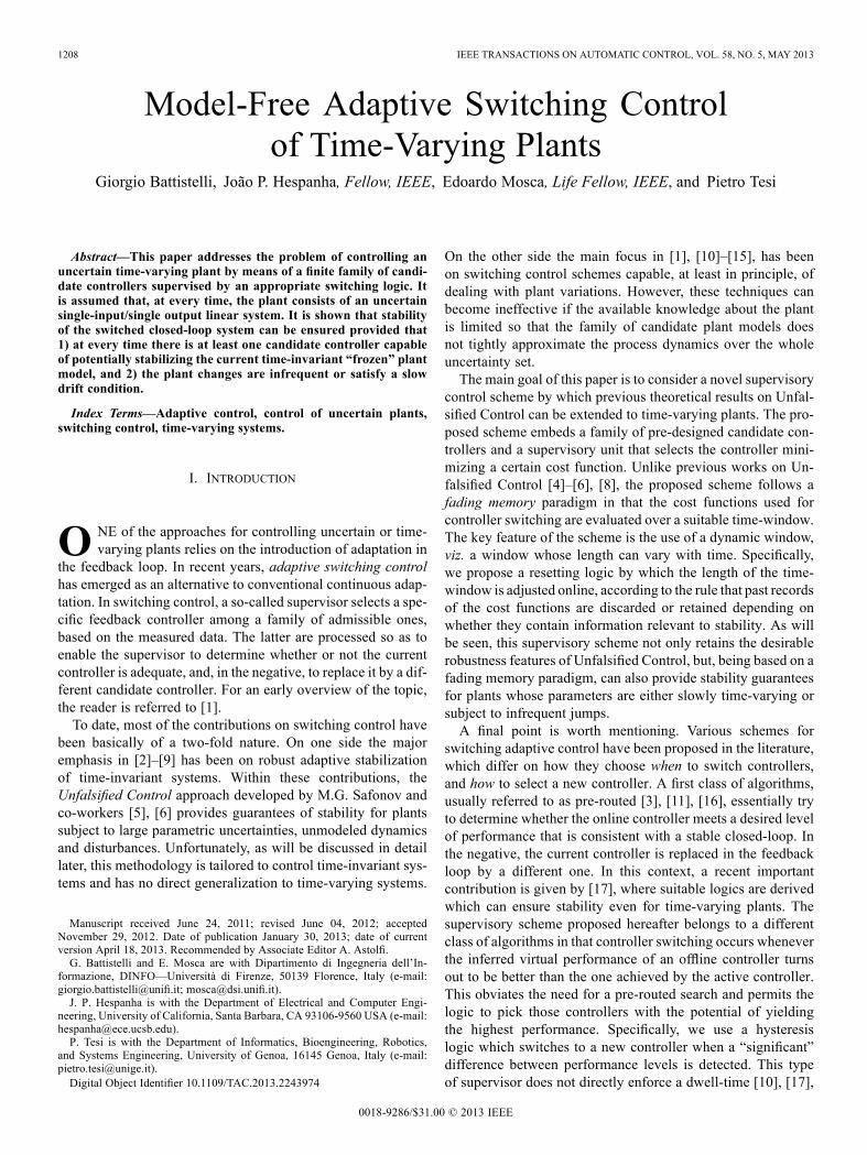
Fig. 3. Supervision based on HSL- . (a) Plant Output. (b) Switchingsequence.

A. Example 1

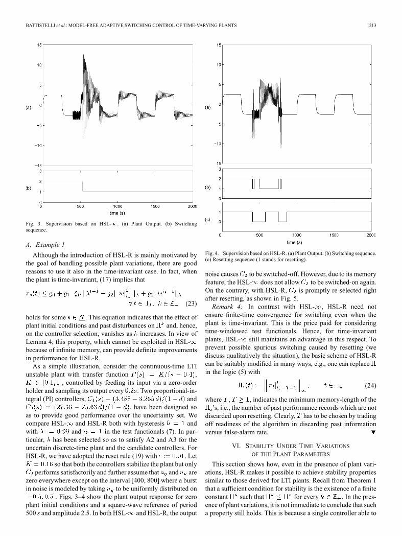
Although the introduction of HSL-R is mainly motivated bythe goal of handling possible plant variations, there are goodreasons to use it also in the time-invariant case. In fact, whenthe plant is time-invariant, (17) implies that

(23)

holds for some . This equation indicates that the effect ofplant initial conditions and past disturbances on and, hence,on the controller selection, vanishes as increases. In view ofLemma 4, this property, which cannot be exploited in HSL-because of infinite memory, can provide definite improvementsin performance for HSL-R.As a simple illustration, consider the continuous-time LTI

unstable plant with transfer function ,, controlled by feeding its input via a zero-order

holder and sampling its output every . Two proportional-in-tegral (PI) controllers, and

, have been designed soas to provide good performance over the uncertainty set. Wecompare HSL- and HSL-R both with hysteresis andwith and in the test functionals (7). In par-ticular, has been selected so as to satisfy A2 and A3 for theuncertain discrete-time plant and the candidate controllers. ForHSL-R, we have adopted the reset rule (19) with . Let

so that both the controllers stabilize the plant but onlyperforms satisfactorily and further assume that and are

zero everywhere except on the interval [400, 800] where a burstin noise is modeled by taking to be uniformly distributed on

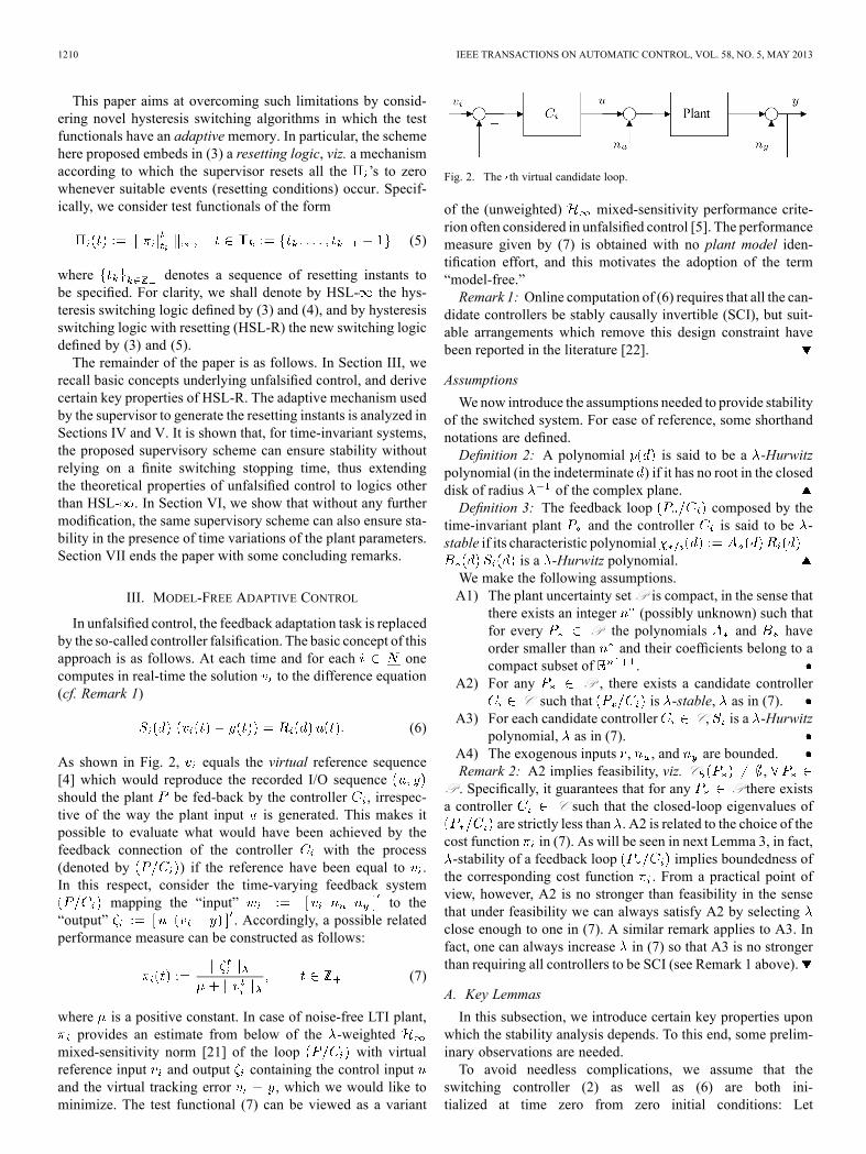
. Figs. 3–4 show the plant output response for zeroplant initial conditions and a square-wave reference of period500 s and amplitude 2.5. In both HSL- and HSL-R, the output

Fig. 4. Supervision based on HSL-R. (a) Plant Output. (b) Switching sequence.(c) Resetting sequence (1 stands for resetting).

noise causes to be switched-off. However, due to its memoryfeature, the HSL- does not allow to be switched-on again.On the contrary, with HSL-R, is promptly re-selected rightafter resetting, as shown in Fig. 5.Remark 4: In contrast with HSL- , HSL-R need not

ensure finite-time convergence for switching even when theplant is time-invariant. This is the price paid for consideringtime-windowed test functionals. Hence, for time-invariantplants, HSL- still maintains an advantage in this respect. Toprevent possible spurious switching caused by resetting (wediscuss qualitatively the situation), the basic scheme of HSL-Rcan be suitably modified in many ways, e.g., one can replacein the logic (5) with

(24)

where , , indicates the minimum memory-length of the’s, i.e., the number of past performance records which are not

discarded upon resetting. Clearly, has to be chosen by tradingoff readiness of the algorithm in discarding past informationversus false-alarm rate.

VI. STABILITY UNDER TIME VARIATIONSOF THE PLANT PARAMETERS

This section shows how, even in the presence of plant vari-ations, HSL-R makes it possible to achieve stability propertiessimilar to those derived for LTI plants. Recall from Theorem 1that a sufficient condition for stability is the existence of a finiteconstant such that for every . In the pres-ence of plant variations, it is not immediate to conclude that sucha property still holds. This is because a single controller able to


Fig. 5. Test functionals ( gray line, black line). (a) Supervision basedon HSL- . (b) Supervision based on HSL-R.

ensure stability over the whole uncertainty set need not exist, theset of stabilizing controllers changing with the plant. As shownhereafter, nonetheless, such a property holds whenever the plantvariations are infrequent or satisfy a slow drift condition.

A. Infrequent Plant Changes

Let denote the sequence of time instants at whicha plant variation occurs, with by convention. Accord-ingly, , , will denote the thtime interval over which the plant is constant. Although we canno longer use in (18) to deduce that the switched systemis stable, Lemma 3 ensures that for every there exists acandidate index such that

(25)

where is as in (18). Thus, for any given accuracy and pro-vided that be large enough, the right hand side of (25) willeventually become smaller than . In this respect, let

Then, if at least two resets occur over , i.e., there is at leastone such that one can use (15) to conclude that attime we have

(26)

where is as in (20). Notice that one single reset wouldnot be sufficient since the bound in (15) depends on bothand . Although Theorem 1 cannot be invoked to concludeclosed-loop stability (since the existence of a finite upperbound for is not apparent from boundedness of

), this implication actually holds.

Lemma 5: Let the HSL-R switched system be based onthe test functionals (7) and reset rule (19). Let A1–A4 hold.Further assume that

(27)

Then, for every , with

(28)

where . Hence, is stable.Proof: See the Appendix.

In the light of Lemma 5, a sufficient condition for stabilityof the switched system is that the minimum interval betweentwo consecutive plant variations (or plant dwell-time) be largeenough to allow the fulfillment of the condition (27). This hap-pens when the plant dwell-time is such that: 1) the transient termin (25) becomes smaller than ; 2) at least two resets occur af-terwards. To see this, recall that items i); and 3) above imply(26). Let now denote the first time instant of , i.e.,

. Accordingly, condition (27) amounts to re-quiring that, for any , is always greater or equalto plus the time needed for two resetting to occur. In this re-spect, using (26) in the definition of one has

Moreover, by simple induction argument, if condition (27) issatisfied up to a certain then, by (28), is an upper boundon the smallest test functional over . In turns, in agreementwith Lemma 4, this implies that after at most stepssubsequent to the two required reset times occur. Summingthe bound on with , we have next result.Theorem 3: Let the HSL-R switched system be based on

the test functionals (7) and the resetting rule (19). Let A1–A4hold. Then, is stable provided that

(29)

holds for every .Notice that the dwell-time depends, through , on the

disturbance amplitude. In words, the larger the level of the dis-turbances, the larger (at least conceptually) the time requiredto select an appropriate controller, hence the larger the intervalrequired between two successive plant variations. Hence,cannot be known a priori unless knowledge on a disturbanceupper bound is assumed. Nonetheless, Theorem 3 guaranteesthat for any disturbance level there exists a sufficiently largeplant dwell-time such that stability is not destroyed.

B. Slow Parameter Drift

Let , , denote the vector of time-varyingparameters composed by the coefficients of and .Consistent with this notation, we can rewrite A1 as requiringthat , for some compact set . Assumenow that the parameter vector takes values inside withbounded variation rate, i.e.,

(30)

where defines the variation rate.


In order to extend the results of the previous section tothis setting, it is convenient to define a collection of sets

, one for each controller index , with the fol-lowing properties:1) all the sets are compact;2) for all , the frozen-time feedback loopis -stable;

3) the collection of sets covers the set withoverlap in the sense that, for any , there existsat least one index such that and

where denotes the boundary of and theEuclidean point-to-set distance.

Thanks to the compactness of the set , by resorting to stan-dard topology arguments, it can be shown that a collection ofsets satisfying such properties always exists under the stated as-sumptions (the existence of a strictly positive being connectedto the existence of a strictly positive Lebesgue number for anyopen cover of the compact set ). More specifically, the fol-lowing result holds.Proposition 1: Under assumptions A1 and A2, there always

exist an overlap and a collection of setsfor which properties 1)–3) hold.

Proof: See the Appendix.Notice that the overlap can be increased by augmenting

the set C with additional controllers. We proceed now to de-rive a bound on cost that is valid on those time intervalsfor which the parameter vector belongs to . To this end,we exploit the well-known fact that, although stability of all thefrozen-time loops , need not imply stabilityof the time-varying loop , , such a prop-erty holds provided that the variation rate be small enough.More specifically, the following result can be stated.Lemma 6: Let the HSL-R switched system be based on

the test functionals (7). Let A1–A4 hold and further assume thaton a given interval the parameter vectoralways remains inside one of the sets . Then, thereexist positive constants , , , and such that, whenthe variation rate does not exceed the threshold , i.e.,

, cost can be upper bounded as

Proof: See the Appendix.Comparing Lemma 6 with its time-invariant counterpart

Lemma 3, it must be noted that the constants andwill now depend on and hence, in general, will be greaterthan the constants and in (17) pertaining to thefrozen-time analysis.As shown hereafter, in view of Proposition 1 and Lemma 6,

conclusions similar to those derived in Section VI-A hold true incase the plant variations satisfy a slow drift conditions. The ideais to derive an inequality of the type given in (25). To this end,we recursively construct a sequence of time instantsas follows: is set equal to 0; given , is defined as the

largest time instant such that there exists at least one indexfor which for any .

In words, if belongs to then denotes the first timeinstant at which a variation in the plant parameter vector cancause to leave . In view of property 3) above, we have that

for any . Hence, we have fromLemma 6 that if then there exists a candidate index

such that

Define

(31)

We therefore obtain forall . This formula clearly parallels the onein (25) for the case of infrequent plant changes. Accordingly, let

, where andfurther assume that

(32)

Since (32) implies that for all ,we have from Theorem 3 that condition (32) is sufficient forstability to hold. Recall now that in order to derive (32) we usedthe assumption that . Combining this latter inequalitywith the fact that impliesbecause is a positive integer, we have the followingstability result in terms of allowed parameter variation rate.Theorem 4: Let the HSL-R switched system be based on

the test functionals (7) and the resetting rule (19). Let A1–A4hold. Then, is stable provided that

(33)

C. Example 2

We consider a simple model of a robot arm [23]. The transferfunction from the control input (motor current) to measurementoutput (motor angular velocity) is

with , , , ,and . The purpose of the control system is to con-trol the angular velocity responses for all admissible values ofthe moment of inertia . Two controllers

andhave been designed. To illus-

trate the advantages of HSL-R over HSL- in the presenceof persistent plant variations, we consider the case whereswitches between 0.0001 (only is stabilizing) to 0.02 (only


Fig. 6. Supervision based on HSL-R. (a) Plant Output. (b) Plant switching se-quence (dotted line) and controller switching sequence (solid line).

Fig. 7. Detail of HSL-R on the time interval [0, 2000] s. (a) Test functionals( gray line, black line). (b) Resetting sequence (1 stands for resetting).

is stabilizing) every 500 s. The parameters andare the same as in Example 1. Fig. 6 depicts the plant outputresponse to a sinusodal reference command and disturbancesmodeled by taking and to be uniformly distributed in

. In accordance with Fig. 7, the resetting mech-anism prevents the test functionals from growing unbounded,thus preserving control reconfiguration. This is not the case forHSL- . In fact, the ever-growing memory of HSL- , whichis reflected in the monotonicity of the test functionals, impliesthat upon each plant variation the cost level necessary for falsi-fying controllers increases. This unavoidably leads to ever-in-creasing transients, as is apparent from Fig. 8. We finally pointout that, although the spikes observed in Fig. 7 are mostly dueto the suddenly unstable dynamics, better transients are likely tobe achieved via bumpless transfer techniques. This constitutesan important area for future investigation.

Fig. 8. Supervision based on HSL- (a) Plant output. (b) Test functionals (gray line, black line).

VII. CONCLUSION

Consideration has been given to the control of uncertain time-varying plants by means of adaptive switching control tech-niques. We have introduced a novel class of algorithms basedon hysteresis switching, which, when combined with appro-priate test functionals, makes it possible to achieve stabilityfor time-varying systems under large plant modeling errors, un-modeled dynamics and persistent disturbances. The character-izing feature of this novel scheme is that the supervisor orches-trates the switching by means of a specially devised mecha-nism which, from time to time, determines whether past dataare still relevant to achieve closed-loop stability. In particular,this mechanism consists of a logic according to which the testfunctionals are reset to zero whenever the recorded data indicatethat the information contained in the test functionals is no longerneeded to achieve stability. Although the major emphasis hasbeen on the stabilization of time-varying systems, simulationresults indicate that this supervisory scheme compares favor-ably with HSL- even when applied to time-invariant systems,since it does not rely on a finite switching stopping-time. Theseresults lend themselves to be extended in various directions.First, the idea of selecting online the memory of the test func-tionals can be extended to more elaborated rules than a simpleresetting logic. As a second point, notice that the motivation forconsidering supervisory schemes based on unfalsified controlwas mainly dictated by the goal of achieving robustness againstlarge modeling uncertainties. Nonetheless, the approach here in-troduced could be used within supervisory schemes alternativeto model-free switching control. In this respect, it is known thatthe adoption of model-based test functionals can significantlyimprove the transients performance [7], [22]. Hence, a naturalquestion arises on whether resetting logics can be adapted to su-pervisory schemes based on multiple models.


APPENDIX

Throughout the appendix, we shall make use of the followingproperties:1) .2) .

3) , .To prove Lemma 2 we use the following result.Proposition 2: Under A1, there exist finite nonnegative

constants , and such that

(34)

Proof of Proposition 2: For any LTI feedback loopwe have

(35)

ByA1, we also get ,for some positive constants and , with .By 1), letting and we get

where the second inequality follows since ,. The proof follows using 2) and recalling

that , .Proof of Lemma 2: Consider an arbitrary and let

, , represent the thsubinterval of over which the switching signal is constant.

Basic Recursive Equation: First, notice that

Consider now an arbitrary . Accordingly, for some ,one has , . Let . By exploiting2) with respect to , with and , we get

(36)

In (36), we made use of the following facts: The second in-equality follows, for some finite positive constant , because

for every and is a -Hurwitzpolynomial; the third inequality is obtained using 1) and letting

; the last inequality follows with since,for all candidate indices, (6) is initialized at time zero from zeroinitial conditions, viz. , . By A3 onesees that the map from to

has bounded –weighted -norm. In particular, since (6) is ini-tialized at time zero from zero initial conditions, it readily fol-lows that , , , and somefinite nonnegative constant . Letting and

, we finally get

(37)

where .Upper-Bound on Data Between Switching: From Lemma

1, we have for every . Then,

(38)

In words, the performance signal related to the switched-on con-troller cannot exceed , apart from the time instants right be-fore switching. Notice that by Lemma 1 this may happen at most-times, since, after switching, no more switching occurs

over .Proof of (12): In order to prove (12) we use (38) and

exploit the results of Proposition 2 at the time instants. Without loss of generality, let , and

as in (34) and, respectively, (38). It is also convenient to letwith and as in (34), and write in more

compact form .Then, combining (34) and (38), we get

(39)

In the second inequality we used the fact that ,while .By induction, it is easy to show that

(40)

Hence, (40) holds true for , and the proof follows by letting.

Proof of Lemma 3: Let , , denote thevector of time-varying parameters composed by the coefficientsof and . Consistently, we can rewrite A1 as requiring that

, for some compact set .By assumption, for all and

some , i.e., for all. Consider now that, under assumption A3, the virtual


references in (6) are well-defined. Thus, combining (6) and (1)we can write , where

(41)Consider next that, for any candidate controller such that

is -stable there exists a polynomial matrixsuch that

(42)

where , , and is suchthat is a -Hurwitz polynomial. Consider now that, byassumption A2, for any there exist a candidate controllerand an open ball around such that is -stable

for all . Thus, an infinite open cover for exists. In turn,in view of assumptions A1 and A2, this implies the existence ofa finite (closed) cover for such that, for each ,all the plants , are stabilized by controller (seethe proof of Proposition 1 below).As a consequence, from (42), it is therefore immediate to con-

clude that there exist positive reals and such that, forany

(43)

holds true where ,

and denotes the -weightednorm of . Hence, (43) holds true over with finite pos-

itive constants and .By ii) with and we have

. By i), we also have

(44)

Consider next that because of the zeroinitial condition constraint, while

the first inequality being obtained from 2) with and. Overall, we get

(45)

where and .Noting that and

, and using 3) with respect toand , with , and , we get

(46)

where . Hence, (17) immediately followsfrom the definition of the ’s.

Proof of Lemma 4: Consider the same notation as in theproof of Lemma 2. Since by assumption for every

, the number of switching on every interval is upperbounded by . Now, using (37) and (38) we obtain

(47)

for every , where

We first derive an upper bound for . By (40)

and, hence,

where the second inequality follows from the defini-tion of admissible resetting times [see (15)]. Considerfurther that , and that

for every ,from which we finally obtain

where is as in (20). Consider now that, because of (47),we have for every , and,hence,

(48)

Indeed, if the latter condition were not satisfied we would thenhave a reset before , contradicting the fact that

. Applying (48) recursively, we get. The claim follows by recalling that

the number of switching is upper bounded by .Proof of Lemma 5: Consider the subsequence of

resets . Notice that, under (27),exists well-defined since and if .

Let and note that .Thus, in order to prove that the switched system is stable, it is


sufficient to prove that the upper bound holds over eachinterval since this implies that the same upper bound willhold over each .Decompose as and first

assume that the interval is nonempty. By definitionnecessarily belongs to , Then, from (25) it follows that

on this interval one has the upper bound . Thus, (12)implies

(49)

Indeed, (49) follows immediately by extending the conclusionsof Lemma 2 to any truncation of a resetting interval ( in thiscase). In addition, by (27) there exists a resetting interval, say

, right before , which is contained into and there-fore such that . Since by virtue of (19) the se-quence of reset times is admissible, the sequenceis such that .Combining this inequality with (49), it follows immediatelythat for every . Fromdefinition of we havefor every . From definition of we therefore obtain

for every . Finally,substituting (26) into (25) it follows that for some index wehave that holds on theinterval from which the upper bound (28) follows. Ifinstead , then and . In such acase (28) follows immediately by (25) and (26).

Proof of Proposition 1: Consider first that, by assump-tion A2, for any there exist a candidate controller

and an open ball around such thatis -stable for all . Thus, an infinite open

cover for exists. Recall now that, by the Heine–Borel the-orem, under assumption A1 any infinite open cover of hasa finite open subcover. Then, this implies the existence of a fi-nite collection of open sets that covers andsuch that, for each , all the plants , are stabi-lized by a common controller . Further, as wellknown, the Lebesgue’s number lemma ensures that there ex-ists a number such that every subset of having diam-eter less than is contained at least in one of the sets

. This implies that the cover isoverlapping in the sense that for any there exists at leastone index such that and . Inorder to conclude the proof, it is now sufficient to pick a positivereal and define, for each , the closed set

In fact, it is immediate to verify that, with such a definition, thecollection of sets satisfies properties 1)–2) byconstruction. As for 3), let . From the overlappingproperty of the cover , we have that for any giventhere exists such that the open ball

is contained in . This, in turn, implies that the openball is contained in the closed set

which is obtained by shrinking the original open set . Then,by definition of , is also contained in the set with

, which implies that .Proof of Lemma 6: Following the same lines as in the proof

of Lemma 3, it can be seen that the signal satisfies the recur-sion

(50)

Let and . Then (50) can berewritten as

(51)

where and. Suppose now that, in a given interval

, one has . Then, for any, the frozen-time characteristic polynomial

of (50) is -Hurwitz. This, in turn, implies that, for any ,the frozen-time characteristic polynomial of(51) is Hurwitz. More specifically, since the set is compact,we have that when all the roots ofalways lie outside a disk of radius with strictlypositive. As a consequence, we can invoke classical results onslowly time-varying systems [24] and conclude that, when thevariation rate does not exceed a given threshold , thenthe system (51) is exponentially stable in the interval . Thus,it is immediate to conclude that, in this case, there exist positivereals and such that, for any

(52)

where . Again, the finiteness of , ,and stems from the compactness of . Note now that, byconstruction

(53)

Hence, inequality (52) can be rewritten as. The rest of the proof

follows along the same lines of the proof of Lemma 3.

REFERENCES

[1] A. S. Morse, “Control using logic-based switching,” in Trends inControl: An European Perspective, A. Isidori, Ed. London, U.K.:Springer, 1995, pp. 69–113.

[2] F. M. Pait and F. Kassab, “On a class of switched, robustly stable,adaptive systems,” Int. J. Adapt. Control Signal Process., vol. 15, pp.213–238, 2001.

[3] D. Angeli and E. Mosca, “Lyapunov-based switching supervisory con-trol of nonlinear uncertain systems,” IEEE Trans. Autom. Control, vol.47, no. 3, pp. 500–505, Mar. 2002.


[4] M. G. Safonov and T. C. Tsao, “The unfalsified control concept andlearning,” IEEE Trans. Autom. Control, vol. 42, no. 6, pp. 843–847,Jun. 1997.

[5] R. Wang, A. Paul, M. Stefanovic, and M. G. Safonov, “Cost de-tectability and stability of adaptive control systems,” Int. J. RobustNonlinear Control, vol. 17, pp. 549–561, 2007.

[6] M. Stefanovic and M. G. Safonov, “Safe adaptive switching control:Stability and convergence,” IEEE Trans. Autom. Control, vol. 53, no.9, pp. 2012–2021, Sep. 2008.

[7] S. Baldi, G. Battistelli, E. Mosca, and P. Tesi, “Multi-model unfalsifiedadaptive switching supervisory control,” Autom., vol. 46, pp. 249–259,2010.

[8] G. Battistelli, E. Mosca, M. G. Safonov, and P. Tesi, “Stability of unfal-sified adaptive switching control in noisy environments,” IEEE Trans.Autom. Control, vol. 55, no. 10, pp. 2425–2429, Oct. 2010.

[9] I. Al-Shyoukh and J. Shamma, “Switching supervisory control usingcalibrated forecasts,” IEEE Trans. Autom. Control, vol. 54, no. 4, pp.705–716, Apr. 2009.

[10] K. Narendra and J. Balakrishnan, “Adaptive control using multiplemodels,” IEEE Trans. Autom. Control, vol. 42, no. 2, pp. 171–187, Feb.1997.

[11] P. V. Zhivoglyadov, R. H. Middleton, and M. Fu, “Localization basedswitching adaptive control for time-varying discrete-time systems,”IEEE Trans. Autom. Control, vol. 45, no. 4, pp. 752–755, Apr. 2000.

[12] B. D. O. Anderson, T. S. Brinsmead, F. D. Bruye, J. P. Hespanha, D.Liberzon, and A. S. Morse, “Multiple model adaptive control, Part 2:Switching,” Int. J. Robust Nonlinear Control, vol. 11(5, pp. 479–496,2001.

[13] J. P. Hespanha, D. Liberzon, and A. S. Morse, “Hysteresis-basedswitching algorithms for supervisory control of uncertain systems,”Autom., vol. 39, pp. 263–272, 2003.

[14] J. P. Hespanha and A. S. Morse, “Stability of switched systems withaverage dwell-time,” in Proc. IEEE Conf. Dec. Control, 1999, pp.2655–2660.

[15] D. Liberzon and L. Vu, “Switching supervisory control fortime-varying plants,” IEEE Trans. Autom. Control, vol. 53, pp.2012–2021, 2010.

[16] M. Fu and B. R. Barmish, “Adaptive stabilization of linear systems viaswitching control,” IEEE Trans. Autom. Control, vol. AC-31, no. 12,pp. 1097–1103, Dec. 1986.

[17] P. Rosa, J. Shamma, C. Silvestre, and M. Athans, “Stability overlay foradaptive control laws,” Autom., vol. 47, pp. 1007–1014, 2011.

[18] A. S. Morse, “Supervisory control of families of linear set-point con-trollers, Part 1: Robustness,” IEEE Trans. Autom. Control, vol. 42, no.11, pp. 1500–1515, Nov. 1997.

[19] D. Angeli and E. Mosca, “Adaptive switching supervisory control ofnonlinear systems with no prior knowledge of noise bounds,” Autom.,vol. 47, pp. 449–457, 2004.

[20] A. S. Morse, D. Q. Mayne, and G. C. Goodwin, “Applications of hys-teresis switching in parameter adaptive control,” IEEE Trans. Autom.Control, vol. 37, no. 9, pp. 1343–1354, Sep. 1992.

[21] A. Datta, “Robustness of discrete-time adaptive controllers: An input-output approach,” IEEE Trans. Autom. Control, vol. 38, no. 12, pp.1652–1657, Dec. 1993.

[22] A. Dehghani, B. Anderson, and A. Lanzon, “Unfalsified adaptive con-trol: A new controller implementation and some remarks,” in Proc.Eur. Control Conf., Kos, Greece, 2007.

[23] K. J. Astrom and B. Wittermark, Adaptive Control, 2nd ed. : Ad-dison-Wesley, 1995.

[24] C. A. Desoer, “Slowly varying discrete system ,” Elec-tron. Lett., vol. 6, no. 11, pp. 339–340, 1970.

Giorgio Battistelli was born in Genoa, Italy, in1975. He received the Laurea degree in electronicengineering and the Ph.D. degree in robotics, bothfrom the University of Genoa, Genoa, Italy, in 2000and 2004, respectively.From 2004 to 2006, he was a Research Associate

in the Dipartimento di Informatica, Sistemistica eTelematica, University of Genoa. He is currentlyan Assistant Professor of automatic control in theDipartimento di Ingegneria dell’Informazione, Uni-versity of Florence. His research interests include

adaptive control, linear and nonlinear estimation, hybrid systems, and datafusion.

Dr. Battistelli is currently an editor of the IFAC journal Engineering Applica-tions of Artificial Intelligence, an associate editor of the IEEE TRANSACTIONSON NEURAL NETWORKS and Learning Systems, and a member of the IEEE Con-trol Systems Society Conference Editorial Board.

João P. Hespanha (S’95–M’98–SM’02–F’08)received the Licenciatura in electrical and computerengineering from the Instituto Superior Técnico,Lisbon, Portugal, in 1991 and the Ph.D. degree inelectrical engineering and applied science from YaleUniversity, New Haven, CT, USA, in 1998.From 1999 to 2001, he was Assistant Professor at

the University of Southern California, Los Angeles,CA, USA. He moved to the University of California,Santa Barbara, in 2002, where he currently holds aProfessor position with the Department of Electrical

and Computer Engineering. He is an Associate Director for the Center for Con-trol, Dynamical-Systems, and Computation (CCDC), Vice-Chair of the Depart-ment of Electrical and Computer Engineering, and a member of the ExecutiveCommittee for the Institute for Collaborative Biotechnologies (ICB). His cur-rent research interests include hybrid and switched systems, the modeling andcontrol of communication networks, distributed control over communicationnetworks (also known as networked control systems), the use of vision in feed-back control, and stochastic modeling in biology.Dr. Hespanha is the recipient of the Yale University’s Henry Prentiss Becton

Graduate Prize for exceptional achievement in research in Engineering andApplied Science, a National Science Foundation CAREER Award, the 2005best paper award at the 2nd International Conference on Intelligent Sensingand Information Processing, the 2005 Automatica Theory/Methodology bestpaper prize, the 2006 George S. Axelby Outstanding Paper Award, and the2009 Ruberti Young Researcher Prize. Dr. Hespanha is an IEEE distinguishedlecturer since 2007. From 2004 to 2007, he was an Associate Editor for theIEEE TRANSACTIONS ON AUTOMATIC CONTROL.

Edoardo Mosca (S’63–M’65–SM’95–F’97–LF-06)received the Dr. Eng. degree in electronics engi-neering from the University of Rome “La Sapienza,”Rome, Italy, in 1963.He then spent four years in the aerospace industry

where he worked on research and development ofadvanced radar systems. Thereafter, from 1968 to1972, he held academic positions at the Universityof Michigan, Ann Arbor, MI, USA, and McMasterUniversity, Hamilton, ON, Canada. Since 1972, hehas been with the University of Florence, Florence,

Italy: until 1974 as an Associate Professor; from 1975 as a full Professor ofControl Engineering; and, from 2012, an Emeritus Professor. He has beenactive in various diversified research fields such as radar signal synthesis andprocessing, radio communications, system identification, adaptive, predictive,switching supervisory control, and detection of performance degradation infeedback-control systems. He is the author of a book, Optimal, Predictive, andAdaptive Control (Prentice Hall, 1995). He has been a journal editor of theEuropean Journal of Control and of the IET Control Theory and Applications;and, currently, of the International Journal of Adaptive Control and SignalProcessing. He is the Italian NMO representative in IFAC where he was aCouncil member from 1996 to 2002, and until 1998 a Council member ofEUCA (European Union Control Association). He is a Fellow of IFAC.

Pietro Tesi received the Laurea degree and the Ph.D.degree in computer and control engineering, bothfrom the University of Florence, Florence, Italy, in2005 and 2010, respectively.In 2006, he worked in the automation industry on

research and development of data acquisition sys-tems. During the Ph.D. degree, he was a short-termPh.D. Scholar at the University of California, SantaBarbara, CA, USA. Since 2010, he has been withboth the University of Florence and the University ofGenoa, Italy. His current research interests include

adaptive control, predictive control, hybrid systems, and adaptive optics.

University of Groningen Model-Free Adaptive Switching ... · Giorgio Battistelli, João P....

Documents

Transcript of University of Groningen Model-Free Adaptive Switching ... · Giorgio Battistelli, João P....