UNIVERSITI PUTRA MALAYSIA

DEVELOPMENT OF ELLIPTIC AND HYPERBOLIC GRID GENERATION

NORZELAWATI ASMUIN

FK 2000 10

DEVELOPMENT OF ELLIPTIC AND HYPERBOLIC GRID GENERATION

By

NORZELAWATI ASMUIN

Thesis Submitted in Fulfilment of the Requirements for the Degree of Master of Science in the Faculty of Engineering

Univer�iti Putra Malaysia

June 2000

DEDICATION

Alhamdulillah, thanks to Allah S.W.t. I have been very fortunate to have

some of the most loving, passionate and supporting husband, Azizan. My great

parents, who always give the best for me the whole of my life. All my sisters and

brothers smile at every accomplishment. My good friends, Kak Ina, Dayang, Kak

Rin and Kak Milah, Aznijar encouraged at every tum and supported me in every

decision. And fmally to Dr. Bambang Basuno thank a lot with your support,

guidance and encouragement.

II

Abstract of thesis presented to the Senate ofUniversiti Putra Malaysia in fulfilment of the requirements for the degree of Master of Science.

DEVELOPMENT OF ELLIPTIC AND HYPERBOLIC GRID GENERATION

By

NORZELAWATI BT. ASMUIN

April 2000 Chairman: Associate Professor Dr ShahNor Basri, P.Eng.

Faculty: Engineering

It has been found that partial differential equations (PDE's) could be used to

efficiently generate high quality structured grids. The grid discretizes the physical

domain to computational domain, typically an array data structure in Fortran. This

study concentrates on elliptic and hyperbolic methods for structured grid generation.

The elliptic method uses the Laplace equations to transfonn the physical domain to

computational domain and fmite difference to generate the grids. Whereas, the

hyperbolic method uses orthogonal relations to solve the PDE's, a marching scheme

to create the grids and then cubic spline interpolations to smoothen grid lines at the

boundaries. C-type and O-type elliptic and hyperbolic grids have been generated for

an airfoil and smooth boundary conditions were obtained in the elliptic method but

not by the hyperbolic method.

iii

Abstrak tesis yang dikemukakan kepada Senat Universiti Putra Malaysia sebagai memenuhi keperluan untuk ijazah Master Sains

PEMBANGUNAN PENJANAAN KEKlSI ELIPS DAN lllPERBOLA

Oleh

NORZELA WATI BT. ASMUIN

Jun 2000 Pengerusi: Profesor Madya Dr ShahNor Basri, P.Eng.

Fakulti: Kejuruteraan

Persamaan pembezaan separa telah dapat digunakan untuk menjana tertisi

berstruktur berkualiti tinggi dengan baik. Tertisi ini terdiskret dari domain fIzikal ke

domain berkomputer, bentuk ini biasanya didalam struktur susunan data didalam

bahasa pengaturcaraan Fortran. Kajian yang dijalankan tertumpu pada penjanaan

tertisi berstruktur menggunakan kaedah elips dan hiperbola. Kaedah elips

menggunakan persamaan Laplace dalam pengubahan domain fIzikal ke bentuk

domain berkomputer serta pembezaan terhingga untuk menjanakan tertisi- tertisi.

Kaedah hiperbola pula menggunakan perhubungan ortogon dalam penyelesaian

persamaan pembezaan separa serta skim rambatan dalam pembentukan tertisi-

tertisi. Seterusnya penentudalaman gelugur kiub digunakan bagi melicinkan garisan

tertisi pada sempadan. Tertisi jenis-C dan jenis-O bagi elips dan hiperbola telah

berjaya dijalankan untuk menjana airfoil. Kaedah sempadan yang Iicin telahpun

diperolehi menggunakan kaedah elips tetapi tidak dengan kaedah hiperbola.

iv

ACKNOWLEDGEMENTS

Alhamdulillah, thanks to Allah S.W.t. and deep thanks to my Supervisor

Associate Prof. Dr. ShahNor Basri to his support, guidance and encouragement

throughout this work.

It is very generous of Dr. Waqar Asrar to his indeed helps through out this

work. I acknowledge the help from Dr. Prithvi Raj Arora, Mr. Faizal, Lt. Kol. Mohd

Ramly Mohd Ajir and the lecturers in Aerospace Engineering, whose support are the

entire technicians in Aerospace Engineering.

v

I certify that an Examination Committee met on 5'h June, 2000 to conduct the final examination of Norzelawati Asmuin on her Master of Science thesis entitled "Development of Elliptic and Hyperbolic Grid Generation" in accordance with Universiti Pertanian Malaysia (Higher Degree) Act 1980 and Universiti Pertanian Malaysia (Higher Degree) Regulations 1981. The Committee recommends that the candidate be awarded the relevant degree. Members of the Examination Committee are as follows:

PRITHVI RAJ ARORA, Ph.D Associate Professor, Faculty of Engineering Universiti Putra Malaysia (Chainnan)

SHAHNOR BASRI, Ph.D Associate Professor, Institut Teknologi Maju Universiti Putra Malaysia (Member)

F AIZAL MUSTAPHA Faculty of Engineering Universiti Putra Malaysia (Member)

LT. KOL. (B) MOHD RAML Y MOHD AnR Faculty of Engineering Universiti Putra Malaysia (Member)

HAZALtMOHA YIDIN, Ph.D, Profes '/ Deputy Dean of Graduate School, Universiti Putra Malaysia

Date: o � JUN 2DOO

vi

This Thesis submitted to the Senate of Universiti Putra Malaysia and was accepted as fulfilment of the requirements for the degree of Master of Science.

vii

�J), Associate Professor Dean of Graduate School, Universiti Putra Malaysia

Date : ,1 3 JUL 2000

DECLARATION

I hereby declare that the thesis is based on my original work except for quotations and citations which have been duly acknowledged. I also declare that it has not been previously or concurrently submitted for any other degree at UPM or other institutions.

viii

(No8� SINTI ASMUIN)

Date: S.'· 2000

TABLE OF CONTENTS

DEDICATION ABSTRACT ABSTRAK ACKNOWLEDGEMENTS APPROVAL SHEETS DECLARATION FORM LIST OF FIGURES LIST OF ABBREVlA TIONS

CHAPTER

I INTRODUCTON Scope and objective of research

II LITERATURE REVIEW Computational fluid dynamic Discretization Grid generation

Elliptic Grid Generation Hyperbolic Grid Generation

Closure

ill BACKGROUND THEORY Introduction Elliptic grid generation method

Laplace equation Poisson equation Control funtions Grid generation Surface grid generation

Hyperbolic grid generation method Transformation relation Differential elements Two-dimensional grid generation Hyperbolic grid generation

Closure

IV COMPUTATIONAL ALGORlTHM Introduction Elliptic grid generation

Matrix and jacobian transformation Discretized elliptic partial differential equation

Programming implementation

ix

Page

ii iii iv v

vi Vlll

xi xii

1 8

9 9 11 14 18 19 20

21 21 21 22 23 28 28 37 37 38 40 41 43 49

50 50 50 51 56 60

Hyperbolic grid generation 60 Hyperbolic grids for airfoils 62 Orthogonality 62 Cell area 63 Marching scheme 63 Boundary value and damper 66 Initial value 68 Cubic spline interpolation 68

Programming implementation 69 Closure 69

V RESULT AND DISCUSSION 7 1 Elliptic grid generation 7 1 Hyperbolic grid generation 73 Closure 75

VI CONCLUSION AND RECOMMENDATIONS 9 1 Conclusion 9 1 Recommendations 92

REFERENCES 94 APPENDIX A 1 0 1 APPENDIXB 1 1 0 BIODATA OF AUTHORS 217

x

LIST OF FIGURES

Figure Page

1 . 1 CFD code development process 2 1 .2 NACA 001 2 4 1 .3 NACA OO12 7 3 .1 The three covariant base vectors 39 3. 2 Orthogonal system 40 4.1 Flowchart of elliptic grid generation 62 4.2 Grid topology 68 4.3 Flowchart of hyperbolic grid generation 71 5 . 1 Circular cylinder model (C-type grid) 77 5.2 Circular cylinder model (O-type grid) 78 5 .3 Convergence rate of circular cylinder 79 5 .4 Elliptic profile (C-type grid) 80 5 .5 Elliptic profile (O-type grid) 8 1 5.6 Convergence rate of Elliptic profile 82 5.7 Airfoil profile (C-type grid) 83 5.8 Airfoil profile (O-type grid) 84 5.9 Convergence rate of airfoil profile 85 5 . 10 Circular cylinder model (C-type grid) 86 5 . 1 1 Circular cylinder model (O-type grid) 87 5 . 12 Elliptic profile (C-type grid) 88 5 . 13 Elliptic profile (O-type grid) 89 5 . 14 Airfoil profile (C-type grid) 90 5 . 1 5 Airfoil profile (O-type grid) 9 1

xi

LIST OF ABBREVIATIONS

r position vector of grid point, ix+jy+kz

iJ,k unit vectors in x,y,z directions

t iteration number

(j) successive-over-relaxation

V quantity

lJ surface boundary condition

I2 outlet boundary condition

s parameter to airfoil

.1R marching rate

x x -axis coordinate in physical domain

y y-axis coordinate in physical domain

� x-axis coordinate in computational domain

1] y-axis coordinate in computational domain

xii

CHAPTER I

INTRODUCTION

Computational aerodynamics, one of the most important technologies in the

development of advanced vehicles, is normally complicated. In many cases the flow

around an arbitrary body shows strongly three dimensional, unsteady and

compressible flow and sometimes with indications of flow discontinuity such as

shock wave. The ability to approach aerodynamics problems using computational

methods, assess the results and make engineering decisions requires very different

skills and attitudes than those associated with fundamental algorithm development.

The major goals of computational aerodynamics typically includes:

• vehicle design, for example, development of optimum airfoil

• performance, for example, estimation of drag

• aeroelasticity analysis, including flutter and divergence

• definition of aerodynamic characteristics for evaluations of stability, control

and handling characteristics.

The governing equations, which describe all features of the flow, are called

the Navier-Stokes equations. The Navier-Stokes equations represent the exact

mathematical model of fluid dynamics. These equations can describe physical flow

phenomena from the simplest case such as the motion of smoke in the air to very

complicated flow pass an array of rotor blades in the compressor of a gas .turbine

engine. As indicated by McCormack (1985), if the Navier-Stokes equations could

be solved exactly, it might change the way current aircraft design has been adopted

2

and significantly reduce the time-consuming wind tunnel testings. Unfortunately,

the Navier-Stokes equations remain still unsolved for most flow problems in

engineering. In response to the difficulties in solving the fundamental equation of

fluid flow, approximate solutions were introduced. There are basically three ways of

solving the flow problems i.e. completely experimental work, numerical modelling

or derivation of approximate solutions.

Two processes must be accomplished in order to generate a complete

computational solution; grid generation and numerical simulation. Grid generation is

the act of specifying the object and the surrounding domain. Grid generation is the

process of specifying the position of all of the grid points that will define both the

objects to be simulated, as well as the surrounding. Grid generation techniques for

simple bodies are fairly straightforward but special techniques must be employed to

handle complex geometries such as aircraft or jet engines. Figure 1.1 shows the

stages of the code development process.

Flow solver Geometry/mesh/grid

-+ • Linear potential .. Post processing Set up for analysis • Full potential

... Graphical

• Euler equation Analysis

• Navier Stoke

Figure 1.1: CFD Code development process

The geometry of the flow domain in computational fluid analysis is usually

complicated. Finite-difference and finite-element solutions both require a discrete

set of points or cells covering the physical field, and the efficiency of the

computation is greatly enhanced if there is some organization to this set. This

organization can be provided by having the discretization defined by the nodes of a

3

curvilinear coordinate system filling the physical field, which is provided by

numerical grid generation.

In both solution technique the most important factor is to maintain a suitable

number of grid points where large or rapid changes are likely to occur. The grid

points are the locations in physical space where the flow variables are actually

computed and stored. These points are usually specified by their position relative to

some fixed point, or origin, and then referenced using their coordinate values. There

will be a number of grid points used to define the surfaces of any body being

simulated, as well as enough grid points to simulate the surrounding. When the

governing equations are solved numerically, the grid points are actually

"transformed" from physical space to computational space. This is done in order to

make it easier to apply numerical boundary conditions.

The grid points are positioned at what appears to be irregular points in

physical space, however in computational space these points are positioned on a

uniform mesh. On a structured mesh, the grid points along each line can be

connected to form a grid line. In unstructured grids, the use of grid lines makes the

visualization of grids and solution much easier. Figure 1 .2, shows a NACA 0012

airfoil structured grids with the same grid visualization using grid points on the grid

point page. The surface of the airfoil is completely defined by grid lines.

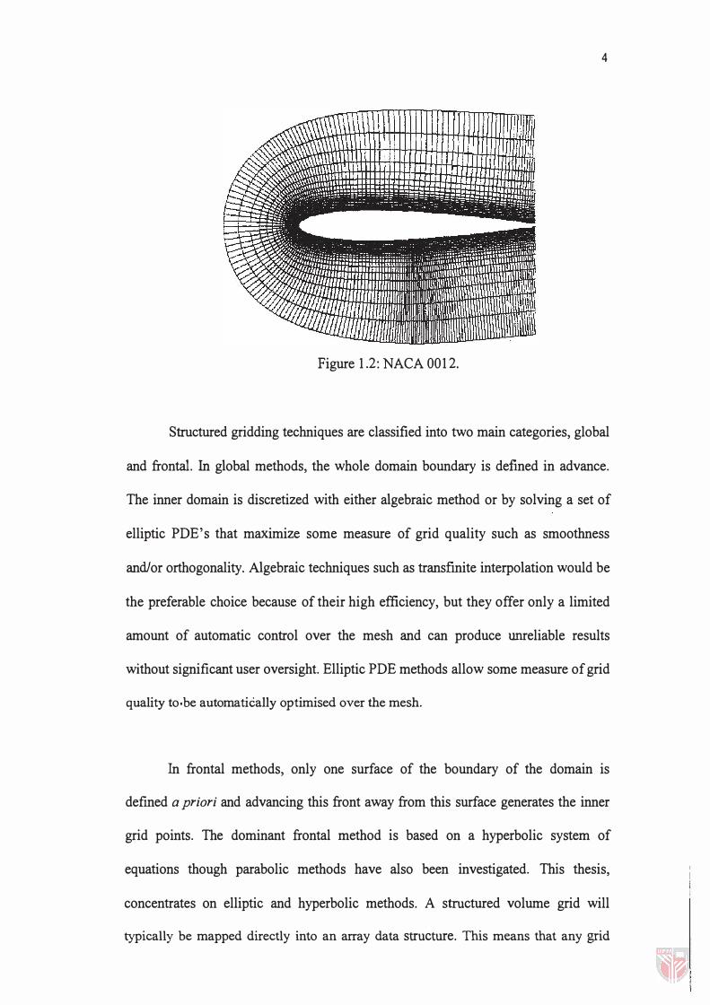
4

Figure 1 .2: NACA 001 2.

Structured gridding techniques are classified into two main categories, global

and frontal. In global methods, the whole domain boundary is defined in advance.

The inner domain is discretized with either algebraic method or by solving a set of

elliptic PDE's that maximize some measure of grid quality such as smoothness

and/or orthogonality. Algebraic techniques such as transfinite interpolation would be

the preferable choice because of their high efficiency, but they offer only a limited

amount of automatic control over the mesh and can produce unreliable results

without significant user oversight. Elliptic PDE methods allow some measure of grid

quality to.be automatically optimised over the mesh.

In frontal methods, only one surface of the boundary of the domain is

defined a priori and advancing this front away from this surface generates the inner

grid points. The dominant frontal method is based on a hyperbolic system of

equations though parabolic methods have also been investigated. This thesis,

concentrates on elliptic and hyperbolic methods. A structured volume grid will

typically be mapped directly into an array data structure. This means that any grid

5

point can trace a path to any other grid point. It has been found that partial

differential equations can be used to efficiently generate high quality structured

grids.

Grid generation progresses in two phases, Surface Grid Generation and

Volume Grid Generation. Defining the surface geometry is often referred to as

defining the solid walls. It refers to the fact that fluid particles cannot pass through a

solid surface, while they are free to move in any direction in other parts of the flow

field. There are two main methods of creating a surface geometry. First, the object to

be simulated has a shape, such as sphere, NACA airfoils, missile geometry and

complete wings. These types of shapes lead to an efficient grid generation process,

with high-quality resulting grids. The second maimer in which surface geometries

are completed is more time-consuming and complex. An aircraft manufacturer will

typically have the design of aircraft stored on their design computers, usually in the

form of CAD data files. These files contain a specification of the aircraft's surface

geometry, but it is not in a form that today's CFD software programmes can

understand. This step often leads to time-delays in the grid generation process, and it

is an area of active research and development in the CFD engineering field.

In order to obtain the forces acting on an aircraft or any other body in motion

through a fluid, it is necessary to physically model both the surface of the body, and

the volume of fluid surrounding the body. This modelling or positioning of the grid

points and grid lines in the surrounding volume is termed volume grid generation. In

order to generate a suitable volume grid for CFD solutions, the grid generation

software must maintain certain criteria. Some of these criteria include finite volume

6

in every computational cell, in which the entire volume must be mapped. Depending

on the type of grid, the grid lines may be required to vary smoothly and intersection

of grid lines should occur at angles as close to 90 degrees as possible. There are two

main classes of volume grids, Structured Volume Grids and Unstructured Volume

Grids. The volume grid generation process for simple geometries, such as wings or

fuselage, is relatively straightforward. Complications arise when attempting to

generate a Volume Grid for a wing-fuselage combination, or other bodies with

realistic shapes.

There are two approaches to generating volume grids for complex

geometries. Either maintain a complicated volume grid generation scheme with

relatively little post-processing effort or use a simpler grid generation scheme with a

complicated grid processing schemes.

Unstructured grids have a definite structure, but they are very flexible and

can be maintained using linear arrays, linked list, binary trees, etc. In unstructured

grids unlike structured grids, a grid point exists in isolation from other points. Grid

cells will have no information about its neighbouring cells. This allows unstructured

grids to easily map very complex geometries and efficiently perform grid adaptation.

Figure 1.3 shows the unstructured two-dimensional volume grid for a NACA 0012.

Unstructured grid generation can be divided into two categories, the

Delaunay Triangulation and Stretching in Delaunay Triangulations. The Delaunay

triangulation prescribes a unique connectivity for a given set of grid nodes. An

7

important problem when stretching a mesh is the control of large angles in the grid

in order to keep the error in the solution bounded.

Figure 1.3: NACA 0012.

An example of unstructured grid generation is automated quadrilateral grid

generation (Hasan, 1996). An all-quadrilateral mesh is generated using the Paving

technique. The geometry of interest is iteratively layered with rows of quadrilateral

elements from the boundary(s) towards the interior. The shape and size of the

elements is controlled through a series of interdependent steps. Care is taken to

minimize the generation of irregular nodes and layer intersections. This technique

can generate a three dimensional mesh in prismatic or two and half dimensional

domains. Mesh quality is estimated quantitatively. Elements are well formed, nearly

square and perpendicular to the boundary.

8

Scope and objective of research

The scope of this research is to investigate the development of elliptic and

hyperbolic grid generation. To achieve this goal, the following is required:

• Study the transformation from physical domain to computational domain for

elliptic and hyperbolic grid generation

• Develop and run the programmes for elliptic and hyperbolic grid generation

• Study the boundary smoothing methods for both grid generation

The report is divided into six chapters. Chapter 1 is the introduction. A

review of literature is presented in Chapter 2. Chapter 3 describes the theory of

elliptic and hyperbolic grid generation. The computational algorithm is presented in

chapter 4. Chapter 5 is concerned with the computational results and discussion. The

conclusions and recommendation are presented in chapter 6.,

CHAPTERll

LITERATURE REVIEW

9

In the late 1970's, the use of computers to solve aerodynamic problems began to

pay off. One early success was the experimental NASA aircraft called RIMA T (Highly

manoeuvrable Aircraft Technology) designed to test concepts of high manoeuvrability

for the next generation of fighter planes. Computational fluid dynamics (CFD)

constitute a new ''third approach" in the philosophical study and development of the

whole discipline of fluid dynamics (Anderson, 1995).

Development of elliptic and hyperbolic grid generation by its very name implies

a coming together of various disciplines each one having a distinct historical

development, and any attempt at a comprehensive review of such a vast subject matter

would require numerous chapters. The survey presented in the subsequent subsections

includes some of the most recent advancement in the respected topics, and the

interested reader may use this as a starting point for further study. In each case,

however, sources of more complete reviews are cited.

Computational fluid dynamic

CFD now stands alongside the wind tunnel in terms of importance in

aerodynamic design. Wind tunnels cannot exist in all the flight regimes such as

hypersonic flight. Its usage by engineering designers involves many thousands of runs

per year, and the rate is increasing. For the simpler aerodynamic flows where viscous

effects are modest, CFD has become the dominant tool of aerodynamic design. The

10

primary role of the wind tunnel for such flows is for validation of a design and for

determination of aerodynamic characteristic over the broad flight envelope. For more

complex flows that are dominated by strong viscous effects, CFD is beginning to make

a contribution (Anderson, 1 995).

The type of computers and algorithms that existed in the 1970's limited all

practical solutions to two-dimensional flows. By 1990, CFD with three-dimensional

flow field solutions were abundant. Some computer programmes for the calculation of

3-D flows have become industry standards, resulting in their use as a tool in the design

process. CFD provides a means to calculate the detailed flow field around a complete

aeroplane configuration, including the pressure distribution over the 3-D surface

(Anderson, 1995).

Modern CFD cuts across all disciplines where the flow of a fluid is important.

There are examples of its applications in the field of automobile and engine design,

industrial manufacturing, civil engineering, environmental engineering and naval

architecture (Anderson, 1995).

CFD is governed by three fundamental principles; conservation of mass,

conservation of energy and Newton's second law, which can be expressed by either

integral or partial differential equations. The strongest force driving the development of

new supercomputers came from the advances of CFD. The earlier high-speed digital

computers were serial machines, capable of one computational operation at a time. The

fmite speed of electrons, close to the speed of light, poses an inherent limitation on the

ultimate execution speed of such serial computers. To overcome this limitation, the

1 1

architecture of the computers was modified, and parallel processors were developed.

(Anderson, 1995).

The advent of CFD has brought in modern fluid dynamics. Therefore, by

studying CFD today, we are participating in an awesome and historic revolution, truly a

measure of the importance of the subject matter.

The various elements of CFD generally include numerical algorithm

development, transition and turbulence modelling, surface modelling and grid

generation, scientific visualisation, and validation methodologies. Advances in these

elements have promoted radically different approaches to the aerodynamic design and

analysis of aerospace vehicles and systems (Hessenius and Richardson, 1991). In the

subsequent section emphasis will be on the basic aspects of the numeric of CFD, that is

discretization.

Discretization

Discretization was first introduced in the German literature in 1955 by W.R.

Wasow, and carried on by Ames in 1965 in his classic book on partial differential

equations. Discretization is the process by which a closed form mathematical

expression, such as function or differential or integral equation involving functions, all

of which are viewed as having infinite continuum of values throughout some domain

(Anderson, 1 989). It can be approximated by analogous but different expressions,

which prescribe values at only a fmite number of discrete points or volumes in the

12

domain. The discretization also must conform to the boundaries of the region in such a

way that boundary conditions can be accurately represented.

The numerical solution of the differential equations governing a complex fluid

dynamics problem requires the introduction of a discretization method. Several

methods have been developed and are currently in use. In the present section the best

idea and techniques used in the development of the finite difference method will be

presented (Evangleos, 1 996).

The numerical solution of the equations of fluid motion require an accurate

defmition of the surface geometry of interest and the generation of an appropriate

surface and flow-field grid. The discretization of the field into a collection of points or

elemental volumes (cells) is required for the numerical solution of the partial

differential equation describing the fluid motion. One method of discretization is the -

method of fmite difference. The finite difference solutions are widely employed in

CFD and are elaborated in the next section.

Finite difference

The finite difference method is the oldest method applied to the numerical

solution of differential equations, and its development is based on the definition of the

derivative and the properties of the Taylor series. In the fmite difference method, the

domain is discretized into a mesh or grid, and the unknown variables exist only at

discrete points called nodes. The derivatives are approximated by differences

(Evangleos, 1996) .