UNIVERSITÀ DEGLI STUDI DI ROMA “TOR … · RPCs as trigger detector for the ATLAS experiment:...
115
UNIVERSITÀ DEGLI STUDI DI ROMA “TOR VERGATA” FACOLTÀ DI SCIENZE MATEMATICHE, FISICHE E NATURALI Dipartimento di Fisica RPCs as trigger detector for the ATLAS experiment: performances, simulation and application to the level-1 di-muon trigger Tesi di dottorato di ricerca in Fisica presentata da Andrea Di Simone Relatori Prof. Rinaldo Santonico Prof.ssa Anna Di Ciaccio Coordinatore del dottorato Prof. Piergiorgio Picozza Ciclo XVII Anno Accademico 2003-2004
Transcript of UNIVERSITÀ DEGLI STUDI DI ROMA “TOR … · RPCs as trigger detector for the ATLAS experiment:...

UNIVERSITÀ DEGLI STUDI DI ROMA“TOR VERGATA”
FACOLTÀ DI SCIENZE MATEMATICHE, FISICHE E NATURALIDipartimento di Fisica
RPCs as trigger detector for the ATLASexperiment: performances, simulation and application to the
level-1 di-muon trigger
Tesi di dottorato di ricerca in Fisica
presentata da
Andrea Di Simone
Relatori
Prof. Rinaldo Santonico
Prof.ssa Anna Di Ciaccio
Coordinatore del dottorato
Prof. Piergiorgio Picozza
Ciclo XVII
Anno Accademico 2003-2004


Contents
Introduction 2
1 The ATLAS experiment 41.1 The Large Hadron Collider . . . . . . . . . . . . . . . . . . . . . 41.2 The Higgs boson at LHC . . . . . . . . . . . . . . . . . . . . . . 61.3 The ATLAS experiment . . . . . . . . . . . . . . . . . . . . . . . 7
1.3.1 Glossary . . . . . . . . . . . . . . . . . . . . . . . . . . 91.3.2 Overall design . . . . . . . . . . . . . . . . . . . . . . . 10
2 The Muon Spectrometer 202.1 Precision chambers . . . . . . . . . . . . . . . . . . . . . . . . . 25
2.1.1 Monitored Drift Chambers . . . . . . . . . . . . . . . . . 262.1.2 Cathode Strip Chambers . . . . . . . . . . . . . . . . . . 27
2.2 Trigger Chambers . . . . . . . . . . . . . . . . . . . . . . . . . . 282.2.1 Thin Gap Chambers . . . . . . . . . . . . . . . . . . . . 28
2.3 The level-1 muon trigger . . . . . . . . . . . . . . . . . . . . . . 30
3 The Resistive Plate Chambers 323.1 Detector description . . . . . . . . . . . . . . . . . . . . . . . . . 323.2 Avalanche growth and signal detection . . . . . . . . . . . . . . . 333.3 The gas mixture . . . . . . . . . . . . . . . . . . . . . . . . . . . 363.4 RPC working regimes and performances . . . . . . . . . . . . . . 37
4 Ageing test of ATLAS RPCs at X5-GIF 394.1 The X5 beam . . . . . . . . . . . . . . . . . . . . . . . . . . . . 404.2 The Gamma Irradiation Facility . . . . . . . . . . . . . . . . . . 414.3 Experimental setup . . . . . . . . . . . . . . . . . . . . . . . . . 434.4 Ageing effects in Resistive Plate Chambers . . . . . . . . . . . . 45
iii

iv Table of contents
4.4.1 Plate resistivity increase . . . . . . . . . . . . . . . . . . 47
4.4.2 Plate surface damage . . . . . . . . . . . . . . . . . . . . 48
4.5 Measurement techniques . . . . . . . . . . . . . . . . . . . . . . 48
4.5.1 Offline analysis . . . . . . . . . . . . . . . . . . . . . . . 48
4.5.2 Plate resistivity measurements . . . . . . . . . . . . . . . 50
4.5.3 Noise level monitoring . . . . . . . . . . . . . . . . . . . 52
4.6 Experimental results . . . . . . . . . . . . . . . . . . . . . . . . 53
4.6.1 Plate resistivity evolution . . . . . . . . . . . . . . . . . . 53
4.6.2 Detector performance . . . . . . . . . . . . . . . . . . . . 55
4.6.3 Gas recirculation . . . . . . . . . . . . . . . . . . . . . . 56
4.6.4 Noise control and damage recovery . . . . . . . . . . . . 58
4.7 Conclusions . . . . . . . . . . . . . . . . . . . . . . . . . . . . . 61
5 F− production in RPCs 655.1 F− concentration measurement . . . . . . . . . . . . . . . . . . . 65
5.1.1 Chemical Potentiometry . . . . . . . . . . . . . . . . . . 65
5.1.2 Activity and concentration . . . . . . . . . . . . . . . . . 66
5.1.3 Free and total ion concentration . . . . . . . . . . . . . . 67
5.2 Experimental setup . . . . . . . . . . . . . . . . . . . . . . . . . 67
5.2.1 Measurement technique . . . . . . . . . . . . . . . . . . 68
5.3 Dependence of the F− production rate on the isobutane concen-tration . . . . . . . . . . . . . . . . . . . . . . . . . . . . . . . . 70
5.4 The effect of the gas flow in F− production and accumulation . . . 72
5.5 F− production as a function of the working current: avalanche andstreamer working regimes . . . . . . . . . . . . . . . . . . . . . . 75
5.6 Conclusions . . . . . . . . . . . . . . . . . . . . . . . . . . . . . 78
6 RPC simulation in the ATLAS offline framework using the Geant4toolkit 806.1 The Geant4 Toolkit . . . . . . . . . . . . . . . . . . . . . . . . . 80
6.2 ATHENA: the ATLAS offline framework . . . . . . . . . . . . . 82
6.3 ATLAS Muon digitization . . . . . . . . . . . . . . . . . . . . . 83
6.4 RPC digitization . . . . . . . . . . . . . . . . . . . . . . . . . . . 83
6.4.1 From hits to digits . . . . . . . . . . . . . . . . . . . . . 83
6.4.2 Cluster simulation . . . . . . . . . . . . . . . . . . . . . 84
6.5 RPC digit validation . . . . . . . . . . . . . . . . . . . . . . . . . 86
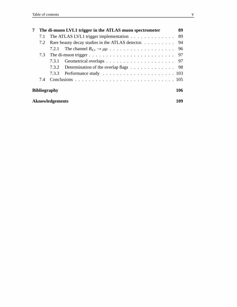
Table of contents v
7 The di-muon LVL1 trigger in the ATLAS muon spectrometer 897.1 The ATLAS LVL1 trigger implementation . . . . . . . . . . . . . 897.2 Rare beauty decay studies in the ATLAS detector. . . . . . . . . . 94
7.2.1 The channel Bd,s → µµ . . . . . . . . . . . . . . . . . . . 967.3 The di-muon trigger . . . . . . . . . . . . . . . . . . . . . . . . . 97
7.3.1 Geometrical overlaps . . . . . . . . . . . . . . . . . . . . 977.3.2 Determination of the overlap flags . . . . . . . . . . . . . 987.3.3 Performance study . . . . . . . . . . . . . . . . . . . . . 103
7.4 Conclusions . . . . . . . . . . . . . . . . . . . . . . . . . . . . . 105
Bibliography 106
Aknowledgements 109


Introduction
The Large Hadron Collider is the proton-proton collider in construction atCERN. It will provide the highest ever realized energy in the center of mass,reaching the value of
√s = 14TeV , thus giving the possibility to investigate a
wide range of physics up to masses of ∼ 1TeV . The most prominent issue isthe search for the origin of the spontaneous symmetry-breaking mechanism inthe electroweak sector of the Standard Model. ATLAS will be one of the fourexperiments installed at the LHC. It has been designed to be a general purposeexperiment, and among its characteristics it has a large stand-alone muon spec-trometer, which allows high precision measurements of the muon momentum. Ageneral overview of the ATLAS experiment and of its muon spectrometer is givenin chapters 1 and 2.
In the muon spectrometer different detectors are used to provide trigger func-tionality and precision momentum measurements. In the pseudorapidity range|η| ≤ 1 the first level muon trigger is based on Resistive Plate Chambers, gas ion-ization detectors which are characterized by a fast response and an excellent timeresolution σt ≤ 1.5ns. The working principles of the Resistive Plate Chamberswill be illustrated in chapter 3.
Given the long time of operation expected for the ATLAS experiment (∼10years), ageing phenomena have been carefully studied, in order to ensure stablelong-term operation of all the subdetectors. Concerning Resistive Plate Cham-bers, a very extensive ageing test has been performed at CERN’s Gamma Irradi-ation Facility on three production chambers. The results of this test are presentedin chapter 4.
One of the most commonly used gases in RPCs operation is C2H2F4 which,during the gas discharge can produce fluorine ions. Being F one of the mostaggressive elements in nature, the presence of F− ions on the plate surface is dan-gerous for the integrity of the surface itself. For this reason a significant effort hasbeen put in the last years to understand the mechanisms of F− production in RPCs
2

operated with C2H2F4-based gas mixtures. The results of the measurements per-formed in the INFN-Roma2 ATLAS laboratories, in collaboration with the Dept.of Science and Chemical Technology of the Univeristy of Rome "Tor Vergata",are presented in chapter 5.
The old Geant3 software toolkit, which has been the de facto standard for highenergy physics simulation in the last 15 years, is being progressively replaced bythe completely re-written toolkit Geant4. The migration from Geant3 to Geant4has required, in the case of the ATLAS experiment, a re-writing from scratch ofmost of the simulation software. In chapter 6 the work done on RPC Geant4 sim-ulation will be described.
Many interesting physics processes to be observed in ATLAS will be char-acterized by the presence of pairs of muons in the final state. For this reason,the ATLAS first level muon trigger has been designed to allow to select di-muonevents. While foreseen in the design of the trigger system, this possibility wasnever intensively tested with the final detector layout. In chapter 7 the first resultsof such a test will be summarized.

Chapter 1
The ATLAS experiment
1.1 The Large Hadron Collider
Figure 1.1: The LHC accelerator chain
The Large Hadron Collider (LHC), is a circular accelerator being built atCERN [1]. It will be hosted in the LEP tunnel, and will accelerate in two separaterings two proton beams up to a center of mass energy of 14 TeV. The machine isalso designed to provide heavy ion collisions (Pb-Pb) at an energy of 1150 TeVin the center of mass, corresponding to 2.76 TeV/u and 7.0 TeV per charge. Thedesign luminosity for pp operation is 1034cm−2s−1, and by modifying the existingantiproton ring (LEAR) into an ion accumulator, the peak luminosity in Pb-Pb op-eration can reach 1027cm−2s−1. Figure 1.1 shows a schematical view of the layout
4

1.2 5
of the machine. The two particle beams can cross in only four points (thus mak-ing their path length identical), which will therefore be the four collision pointsavailable for experiments. At the crossing point the angle between the beams willbe 200µrad.
The two high luminosity insertions in point 1 and point 5, diametrically op-posed, will host the experiments ATLAS and CMS respectively. Two more exper-iments, one aimed at the study of heavy ions collisions (ALICE) and one designedto perform accurate studies on B physics (LHCb) will be located in point 2 andpoint 8.
p-p operation. The beams in the LHC will contain 2835 bunches of 1011 protonseach per beam. The existing CERN accelerator chain, illustrated in figure 1.1,will be used as injection system for the LHC. The bunches, with an energy of26 GeV are formed in the PS, and are characterized by a 25ns spacing. Threetrains of 81 bunches, corresponding to a total charge of 2.43 1013 protons, arethen injected in the SPS on three consecutive PS cycles, thus filling 1/3 of theSPS circumference. The resulting beam is accelerated to 450 GeV before beingtransferred to the LHC. This cycle has to be repeated 12 times in order to fill boththe LHC counter-rotating beams.
Heavy ion operation. In the case of Pb-Pb beams, the optimal bunch spacingwould be 134.7ns at the LHC collision energies. In order to permit the protonexperiments to trigger ion collisions, and ALICE to trigger on protons, it was de-cided to reduce this spacing to 125ns, which is multiple of the 25ns spacing usedin proton operation. The primary source of ions is a lead linac, producing, at arate of 10 Hz, a 60µs, 22µA pulse of Pb54+ at 4.2 MeV/u. Each pulse is injected inLEAR, where it is cooled in 0.1 s using electron cooling. After the injection of 20pulses the beam, containing 1.2 1019 ions divided in four batches, is acceleratedto 14.8 MeV/u and then sent to the PS. In the PS the four bunches, occupying aquarter of the machine’s circumference, are accelerated to a momentum of 6.15GeV/c/u, and the bunch spacing is tuned at 125 ns. The four bunches are trans-ferred to the SPS in one single batch, and 13 consecutive such batches are storedin succession in the SPS, accelerated and then injected in the LHC. The injectorcycle uses 152 PS cycles, 12 SPS cycles for a total filling time of 9.8 min for eachLHC ring.

6 Chapter 1. The ATLAS experiment
1.2 The Higgs boson at LHC
As shown in figure 1.3 the total production cross section for a Higgs bosonis greater than 100 f b in all its estimated mass range. This implies that in oneyear of data taking at the LHC more than 103 Higgs events will be producedat low luminosity and more than 104 during high luminosity operation. Figure1.2 shows the Feynman diagrams of the principal production mechanisms for theHiggs boson.
The gluon fusion process has the highest cross section over all the mass range.For mH ∼ 1TeV the Z or W fusion process becomes comparable with the gluonfusion. The production associated with a pair has smallest cross sections, but thedecay channels of the top quark or of the W or Z boson can generate very cleanexperimental signatures.
The coupling of the Higgs boson to a particle has a dependence on the mass ofthe particle. As a consequence, the branching ratios of the Higgs are highest fordecays in heavy particles. Figure 1.4 shows the branching ratios of the Higgs as afunction of mH. The Higgs decay channels, their backgrounds and their signaturescan be summarized as follow, as a function of mH:
• mH < 130GeV . In this mass region H → bb is the most favorite channel,being the bb the heaviest fermion pair accessible to the Higgs. This decaychannel is affected by the background of bb coming from other processes.The associated production channels can be studied through the identificationof the leptons produced in the decays of the t or of the W or Z bosons.The channel H → γγ is rarer, but it has a clear experimental signature: theseevents are characterized by two isolated photons with high pT . Its detectionrequires a good identification of photons and and a high energy resolution.The background for this channel is mainly due to q q → γγ and gg → γγ
processes.
• 130GeV < mH < 2mZ. One of the most promising channels in this regionis H → ZZ∗ → 4l. The background for this kind of processes come fromtt → Wb + Wb → lν + lν c + lν + lνc and Zbb → 4l, and can be reducedrequiring at least a pair l+l− with a mass compatible with mZ and rejectingevents with secondary vertices.At mH = 170GeV the dominant decay channel becomes H → WW ∗. In thiscase the signal H → WW∗ → lνlν will be studied, thus requiring a goodresolution in transverse missing energy.
1.3 7
• mH ≥ 2mZ. At these masses, the channel H → 4l becomes accessible. Ithas an extremely clean signature, thanks to the high pT of the four leptons.At mH > 600GeV , also the channels H → ZZ → llνν and H → WW →lν jet jet can be studied.
1.3 The ATLAS experiment
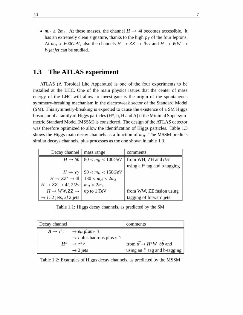
ATLAS (A Toroidal Lhc Apparatus) is one of the four experiments to beinstalled at the LHC. One of the main physics issues that the center of massenergy of the LHC will allow to investigate is the origin of the spontaneoussymmetry-breaking mechanism in the electroweak sector of the Standard Model(SM). This symmetry-breaking is expected to cause the existence of a SM Higgsboson, or of a family of Higgs particles (H±, h, H and A) if the Minimal Supersym-metric Standard Model (MSSM) is considered. The design of the ATLAS detectorwas therefore optimized to allow the identification of Higgs particles. Table 1.3shows the Higgs main decay channels as a function of mH. The MSSM predictssimilar decays channels, plus processes as the one shown in table 1.3.
Decay channel mass range comments
H → bb 80 < mH < 100GeV from WH, ZH and ttHusing a l± tag and b-tagging
H → γγ 90 < mH < 150GeVH → ZZ∗ → 4l 130 < mH < 2mZ
H → ZZ → 4l, 2l2ν mH > 2mZ
H → WW, ZZ → up to 1 TeV from WW, ZZ fusion using→ lν 2 jets, 2l 2 jets tagging of forward jets
Table 1.1: Higgs decay channels, as predicted by the SM
Decay channel comments
A→ τ+τ− → eµ plus ν ’s→ l plus hadrons plus ν ’s
H± → τ±ν from tt → H±W∓bb and→ 2 jets using an l± tag and b-tagging
Table 1.2: Examples of Higgs decay channels, as predicted by the MSSM

8 Chapter 1. The ATLAS experiment
(a) t
t
t
g
g
H
(b) W(Z)
W(Z)
q(q′) q(q′)
q q
H
(c) t
t
g t
g t
H
(d)W(Z)
q
q
H
W(Z)
Figure 1.2: Feynman diagrams of the main production processes of the Higgsboson: gluon fusion (a), Z or W fusion (b), production associated with a tt pair (c)or with a Z or W boson (d).
(pp→H+X) [pb]√s = 14 TeV
Mt = 175 GeV
CTEQ4Mgg→H
qq→Hqqqq
_’→HW
qq_→HZ
gg,qq_→Htt
_
gg,qq_→Hbb
_
MH [GeV]0 200 400 600 800 1000
10-4
10-3
10-2
10-1
1
10
10 2
0 100 200 300 400 500 600 700 800 900 1000
Figure 1.3: Production cross sections for the Higgs boson at LHC as a function ofthe mass of the boson.

1.3 9
BR
for
SM
Hig
gs
_bb
+
cc_
gg
WW
ZZ
tt-
Z
50 100 200 500 100010
-3
10-2
10-1
1140 GeV
Higgs Mass (GeV)
Figure 1.4: Higgs branching ratios as a function of the Higgs mass.
Figure 1.5 shows the expected significance of a Higgs signal as a function ofmH.
1.3.1 Glossary
In the ATLAS standard reference frame, the z-axis is oriented along the beam,while the x-y plane is perpendicular to the beam axis. The x positive direction isthe one pointing to the center of the LHC, and the y axis is pointing upwards.
The angle measured around the beam axis is called φ, or azimuthal, and theangle with respect to the beam axis is called θ, or polar. The pseudorapidity η isdefined as η = − ln tan θ
2 . In the following, transverse momentum (pT ), transverseenergy (ET ) and transverse missing energy (Emiss
T ) refer to the quantities measuredin the x-y plane.
The detector is divided along z in three parts: side A is the side with z > 0,side C is at z < 0 and side B is the plane z = 0. Figure 1.6 shows the layout of thesubdetectors in the ATLAS experiment.

10 Chapter 1. The ATLAS experiment
1
10
10 2
102
103
mH (GeV)
Sig
nal s
igni
fica
nce
H → + WH, ttH (H → ) ttH (H → bb) H → ZZ(*) → 4 l
H → ZZ → ll H → WW → ljj
H → WW(*) → ll
Total significance
5
∫ L dt = 100 fb-1
ATLAS
Figure 1.5: Expected discovery potential for the Higgs boson of the ATLAS ex-periment for an integrated luminosity of 100 f b−1, as a function of mH.
1.3.2 Overall design
In order to achieve the necessary sensitivity to the physics processes to bestudied at the LHC, the ATLAS detector ha been designed to provide:
• Electron and photon identification and measurements, using a very perfor-mant electromagnetic calorimetry.
• Accurate jet and missing transverse momentum measurements, using, in ad-dition to electromagnetic calorimeters, the full-coverage hadronic calorime-try.
• Full event reconstruction at low luminosity.
• Efficient tracking also at high luminosity, with particular focus on high-pT
lepton momentum measurements.
• Large acceptance in pseudorapidity, and almost full coverage in φ.

1.3 11
Figure 1.6: The ATLAS detector
A superconducting solenoid generates the magnetic field in the inner region ofthe detector, while eight large air-core superconducting toroids are placed outsidethe calorimetric system, and provide the magnetic field for the external muon

12 Chapter 1. The ATLAS experiment
spectrometer.
The Magnet System
The overall dimensions of the ATLAS magnet system are 26m in length and22m in diameter. In the end-cap region, the magnetic field is provided by twotoroid systems (ECT) inserted in the barrel toroid (BT) and lined up with the cen-tral solenoid (CS). The CS provides the inner trackers with a field of 2T (2.6Tat the solenoid surface). Being the CS in front of the calorimetric system, its de-sign was carefully tuned in order to minimize the material and not to produce anydegradation of the calorimeter performance. As a consequence of this constraints,the CS and the barrel EM calorimeter share the same vacuum vessel. The operat-ing current of the solenoid is 7.6kA.
The magnetic field generated by the BT and ECT have peak values of 3.9 and4.1 T respectively. The eight coils of the BT, as wheel as the 16 coils of the ECTare electrically connected in series and powered by 21kA power supply.
The magnets are cooled by a flow of helium a 4.5K.All the coils are made of a flat superconducting cable located in an aluminum
stabilizer with rectangular shape. The aluminum used in the CS is doped in orderto provide higher mechanical strength.
The Inner Detector
The Inner Detector (ID) is entirely contained inside the Central Solenoid,which provides a magnetic field of 2T . The high track density expected to char-acterize LHC events calls for a careful design of the inner tracker. In order toachieve the maximum granularity with the minimum material, it has been chosento use two different technologies: semiconductor trackers in the region around thevertex are followed by a straw tube tracker. Figure 1.7 shows a schematical viewof the ID.
The semiconductor tracker is divided in two subdetectors: a pixel detector anda silicon microstrip detector (SCT). The total number of precision layers is limitedby the quantity of material they introduce and also because of their cost. In theresulting setup, a track typically crosses three pixel layers and eight SCT layers(corresponding to four space points). The three pixel layers in the barrel have aresolution of 12µm in Rφ and 66µm in Z. In the endcaps the five pixel disks oneach side provide measurements in Rφ and R with resolutions of 12µm and 77µm

1.3 13
TRT
Pixels SCT
Barrelpatch panels
Services
Beam pipe
Figure 1.7: ATLAS inner detector
respectively. The innermost layer of pixel detectors in the barrel is placed at about4cm from the beam axis, in order to improve the secondary vertex measurementcapabilities.
The SCT detector uses small angle (40mrad) stereo strips to measure positionsin both coordinates (Rφ, Z for the barrel and Rφ,R for the endcaps). For each de-tector layer one set of strips measures φ. The resolutions obtained in the barrel are16µm and 580µm for Rφ and Z respectively, while in the endcaps the resolutionsare 16µm in Rφ and 580µm in R.
The straw tubes are parallel to the beam in the barrel while in the endcapsthey are placed along the radial direction. Each straw tube has a resolution of170µm, and each track crosses about 36 tubes. In addition to this, the straw tubetracker can also detect the transition-radiation photons emitted by electrons cross-ing the xenon-based gas mixture of the tubes, thus improving the ATLAS particleidentification capabilities.
The EM Calorimeter
The EM calorimeter is divided in three parts: one in the barrel (|η|<1.7) andtwo in the endcaps (1.375 < |η|<3.2). The barrel calorimeter is divided in two halfbarrels, with a small (6mm) gap between them at z = 0. The endcap calorimetersare made up of two coaxial wheels each. The layout of the EM calorimeter, to-gether with the hadronic one, is illustrated in figure 1.8.
The EM calorimeter is a Liquid Argon detector with lead absorber plates andKapton electrodes. In order to provide a full coverage in φ, an accordion geometry

14 Chapter 1. The ATLAS experiment
Calorimeters
Calorimeters
Calorimeters
Calorimeters
Hadronic Tile
EM Accordion
Forward LAr
Hadronic LAr End Cap
Figure 1.8: The ATLAS calorimeters
was chosen for the internal flayout of the calorimeter. The lead absorber layershave variable thickness as a function of η and has been optimized to obtain thebest energy resolution. The LAr gap on the contrary has a constant thickness of2.1mm in the barrel. The total thickness is >24X0 in the barrel and >26X0 in theendcaps.
In the region with |η| < 2.5 the EM calorimeter is longitudinally divided inthree sections. The first region, is meant to work as a preshower detector, pro-viding particle identification capabilities and precise measurement in η. It has athickness of ∼6X0 constant as a function of η, is read out with strips of 4mm in theη direction.
The middle section is divided into towers of size ∆φ × ∆η = 0.025 × 0.025(∼ 4 × 4cm2 at η=0) with square section. At the end of this section the calorime-ter has a total thickness of ∼24X0. The third section has a lower granularity in η(∼ 0.05).
The calorimeter cells point towards the interaction region over the complete

1.3 15
η range, and the total number of channels is ∼ 190000. A schematic layout of acalorimeter cell is shown in figure 1.9.
= 0.0245
= 0.02537.5mm/8 = 4.69 mm = 0.0031
=0.0245x4 36.8mmx4 =147.3mm
Trigger Tower
TriggerTower = 0.0982
= 0.1
16X0
4.3X0
2X0
1500
mm
470
mm
= 0
Strip towers in Sampling 1
Square towers in Sampling 2
1.7X0
Towers in Sampling 3 = 0.0245 0.05
Figure 1.9: Schematic layout of an ATLAS accordion calorimeter cell.
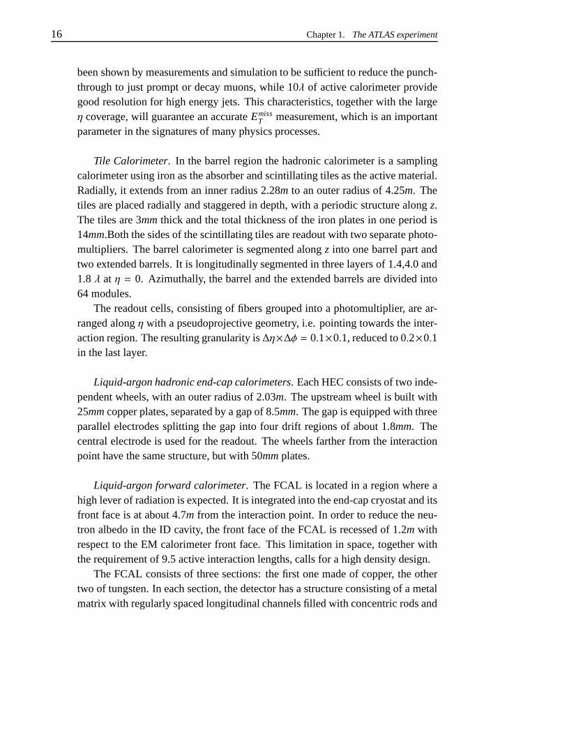
The Hadronic Calorimeter
The region with |η| < 4.9 is covered by the hadronic calorimeters using differ-ent techniques, taking into account the varying requirements and radiation envi-ronment over this large η range. The range |η| < 1.7, corresponding to the barrelcalorimeter, is equipped with a calorimeter (TC) based on the iron/scintillating-tile technology. Over the range ∼ 1.5 < |η| < 4.9, Liquid Argon calorimeters werechosen. In this region the hadronic calorimetry is segmented into an HadronicEnd-Cap Calorimeter (HEC), extending up to |η| < 3.2 and a High Density For-ward Calorimeter (FCAL) covering the region with highest |η|. Both the HEC andthe FCAL are integrated in the same cryostat housing the EM end-caps calorime-try. The overall layout of the ATLAS hadronic calorimeters is shown in figure 1.8.
The thickness of the calorimeter has been carefully tuned in order to providegood containment of hadronic showers and reduce to the minimum the punch-through into the muon system. At η = 0 the total thickness is 11 interactionlengths (λ), including the contribution from the outer support (∼ 1.5λ). This has
16 Chapter 1. The ATLAS experiment
been shown by measurements and simulation to be sufficient to reduce the punch-through to just prompt or decay muons, while 10λ of active calorimeter providegood resolution for high energy jets. This characteristics, together with the largeη coverage, will guarantee an accurate Emiss
T measurement, which is an importantparameter in the signatures of many physics processes.
Tile Calorimeter. In the barrel region the hadronic calorimeter is a samplingcalorimeter using iron as the absorber and scintillating tiles as the active material.Radially, it extends from an inner radius 2.28m to an outer radius of 4.25m. Thetiles are placed radially and staggered in depth, with a periodic structure along z.The tiles are 3mm thick and the total thickness of the iron plates in one period is14mm.Both the sides of the scintillating tiles are readout with two separate photo-multipliers. The barrel calorimeter is segmented along z into one barrel part andtwo extended barrels. It is longitudinally segmented in three layers of 1.4,4.0 and1.8 λ at η = 0. Azimuthally, the barrel and the extended barrels are divided into64 modules.
The readout cells, consisting of fibers grouped into a photomultiplier, are ar-ranged along η with a pseudoprojective geometry, i.e. pointing towards the inter-action region. The resulting granularity is ∆η×∆φ = 0.1×0.1, reduced to 0.2×0.1in the last layer.
Liquid-argon hadronic end-cap calorimeters. Each HEC consists of two inde-pendent wheels, with an outer radius of 2.03m. The upstream wheel is built with25mm copper plates, separated by a gap of 8.5mm. The gap is equipped with threeparallel electrodes splitting the gap into four drift regions of about 1.8mm. Thecentral electrode is used for the readout. The wheels farther from the interactionpoint have the same structure, but with 50mm plates.
Liquid-argon forward calorimeter. The FCAL is located in a region where ahigh lever of radiation is expected. It is integrated into the end-cap cryostat and itsfront face is at about 4.7m from the interaction point. In order to reduce the neu-tron albedo in the ID cavity, the front face of the FCAL is recessed of 1.2m withrespect to the EM calorimeter front face. This limitation in space, together withthe requirement of 9.5 active interaction lengths, calls for a high density design.
The FCAL consists of three sections: the first one made of copper, the othertwo of tungsten. In each section, the detector has a structure consisting of a metalmatrix with regularly spaced longitudinal channels filled with concentric rods and

1.3 17
tubes. The rods are at positive high voltage, while the tubes and the matrix aregrounded. The LAr in the gap between is the sensitive medium.
The Trigger/DAQ system
The ATLAS trigger and DAQ system is described in figure 1.10. The triggeris organized in three levels, called LVL1, LVL2 and EF (Event Filter).
LVL2
LVL1
Rate [Hz]
40 106
104-105
CALO MUON TRACKING
Readout / Event Building
102-103
pipeline memories
MUX MUX MUX
derandomizing buffers
multiplex data
digital buffer memories
101-102
~ 2 s(fixed)
~ 1-10 ms(variable)
Data Storage
Latency
~1-10 GB/s
~10-100 MB/s
LVL3processor
farm
Switch-farm interface
Figure 1.10: Block diagram of the ATLAS Trigger/DAQ system
LVL1 [7] acts on reduced granularity (∆η × ∆ϕ = 0.1 × 0.1) data from thecalorimeters and the muon spectrometer; its decision is based on selection criteriaof inclusive nature. Example menus are shown on tables 1.3 and 1.4 with thecorresponding trigger rate expected at low and high luminosity.
LVL1, whose block diagram is shown in figure 1.11 is divided into four parts:the calorimeter trigger, the muon trigger, the central trigger processor, which isin charge of taking the final decision, and the TTC (Timing, Trigger and Controldistribution system), which is responsible for the distribution of the trigger outputto the front-end electronics of the subdetectors.
The main task of the LVL1 trigger system is to correctly identify the bunchcrossing of interest. In ATLAS this is not a trivial task, since the dimensions ofthe muon spectrometer imply times of flight larger than 25ns and the shape of

18 Chapter 1. The ATLAS experiment
Muon Trigger / CTPInterface
Central Trigger Processor
TTC
Muon Trigger(RPC based)
Muon Trigger(TGC based)
Front-end Preprocessor
Cluster Processor(electron/photon andhadron/tau triggers)
Jet/Energy-sumProcessor
Calorimeter Trigger Muon Trigger
Endcap Barrel
Figure 1.11: Block diagram of the ATLAS LVL1 Trigger system
calorimeter signals extends over many bunch crossings. The LVL1 latency (timespent to take and distribute the decision) is 2µs, with an output rate of 75kHz,increasable up to 100kHz (limit imposed by the design of the front-end electron-ics).
Events selected by LVL1 are stored in ROBs, Read Out Buffers, waiting forthe LVL2 decision. In case of positive decision, events are fully reconstructedand stored for the final decision of the Event Filter. The LVL2 reduces the triggerrate to 1kHz, using also information from the Inner Detector. It has access to thefull data of the event, with full precision and granularity, but its decision is takenconsidering only data from a small region of the detector, i.e the ROI (Region OfInterest) identified by the LVL1. Depending on the event, the latency of LVL2 canvary from 1ms to 10ms.
The final trigger decision is taken by the Event Filter by means of off-linealgorithms; the acquisition rate is required to be less than 100Hz for events of∼ 1Mbyte.

1.3 19
Table 1.3: Example of LVL1 trigger menu (L = 1034cm−2s−1).
Trigger Rate(kHz)Single muon, pt >20 GeV 4Pair of muons, pt >6 GeV 1Single isolated EM cluster, Et >30 GeV 22Pair of isolated EM clusters, Et >20 GeV 5Single jet, Et >290 GeV 0.2Three jets, Et >130 GeV 0.2Four jets, Et >90 GeV 0.2Jet, Et >100 GeV AND missing Et >100 GeV 0.5Tau, Et >60 GeV AND missing Et >60 GeV 1Muon, pt >10 GeV AND isolated EM cluster, Et >15 GeV 0.4Other triggers 5Total '40
Table 1.4: Example of LVL1 trigger menu (L = 1033cm−2s−1).
Trigger Rate(kHz)Single muon, pt >6 GeV 23Single isolated EM cluster, Et >20 GeV 11Pair of isolated EM clusters, Et >15 GeV 2Single jet, Et >180 GeV 0.2Three jets, Et >75 GeV 0.2Four jets, Et >55 GeV 0.2Jet, Et >50 GeV AND missing Et >50 GeV 0.4Tau, Et >20 GeV AND missing Et >30 GeV 2Other triggers 5Total '40

Chapter 2
The Muon Spectrometer
One of the most promising signatures of physics at the LHC is the presence ofhigh momentum final state muons. To exploit this potential, the ATLAS detectorprovides a high resolution muon spectrometer with stand-alone trigger, allowingthe high precision measurement of transverse momentum over a wide range ofpseudorapidity and azimuthal angle. Figures 2.1 and 2.2 show the conceptuallayout of the spectrometer [2]. It is based on the deflection of muon tracks ina system of three large superconducting air-core toroid magnets. In the regionwith |η| < 1.0 the magnetic field is generated by a large barrel magnet constructedby eight superconducting coils surrounding the barrel hadronic calorimeter. For1.4 < η < 2.7 muons are bent by the field produced by two small end-cap magnetsinserted at both end of the barrel toroid. In the transition region (1.0 < η < 1.4)muon bending is provided by a combination of the barrel and end-cap fields.
Physics requirements The muon spectrometer has been designed to provideaccurate momentum measurements over a wide energy scale. It will detect thesignatures of Standard Model and Supersymmetric Higgs, with the possibilityto provide also accurate measurements of low energy muons, such as the onesproduced in processes of interest for CP violation studies or B physics. The mostimportant parameters that have been optimized for maximum physics reach are:
• Resolution. Momentum and mass resolution at the level of 1% are requiredfor reliable charge identification and for reconstruction of two- and four-muon final states on top of high background levels.
20

2.0 21
2
4
6
8
10
12 m
00
Radiation shield
MDT chambers
End-captoroid
Barrel toroid coil
Thin gap chambers
Cathode strip chambers
Resistive plate chambers
14161820 21012 468 m
Figure 2.1: Side view of one sector of the muon spectrometer.
• Second coordinate measurement. Along the non-bending projections, muontracks need to be detected with a resolution of 5-10mm in order to obtain asafe track reconstruction.
• Rapidity coverage. The pseudorapidity coverage up to |η| ∼ 3, together withthe good hermeticity, is important for all physics processes, in particular forrare high-mass processes.
• Trigger Selectivity. High mass states, such as the ones that will be studied atthe LHC nominal luminosity call for trigger thresholds of 10-20 GeV, whilelower thresholds (∼ 5GeV) are necessary to study CP violation and beautyphysics.
• Bunch-crossing identification. the LHC bunch-crossing interval of 25ns setsthe scale for the required time resolution of the first-level trigger system.
Background conditions The expected background can be classified in two cat-egories:
• Primary background. This background is principally due to primary col-lision products penetrating in the spectrometer through the calorimeters,which are correlated in time with the p-p interaction. Sources of primarybackground are semileptonic decays of light (π,K→ µX) and heavy (c,b,t→

22 Chapter 2. The Muon Spectrometer
End-captoroid
Barrel toroidcoils
Calorimeters
MDT chambersResistive plate chambers
Inner detector
Figure 2.2: Transverse view of the spectrometer.
µX) flavors, gauge bosons decays (W,Z,γ∗ → µX), shower muons andhadronic punch-through.
• Radiation background. This background consist mostly of neutrons andphotons in the 1 MeV range, produced by secondary interactions in theforward calorimeter, shielding material, the beam pipe and the machine el-ements. Low-energy neutrons, which are an important component of thehadronic absorption process, escape the absorber and produce a gas of low-energy photon background through nuclear n-γ processes. This backgroundenters the spectrometer from all directions and is no more correlated in timewith the bunch crossing.
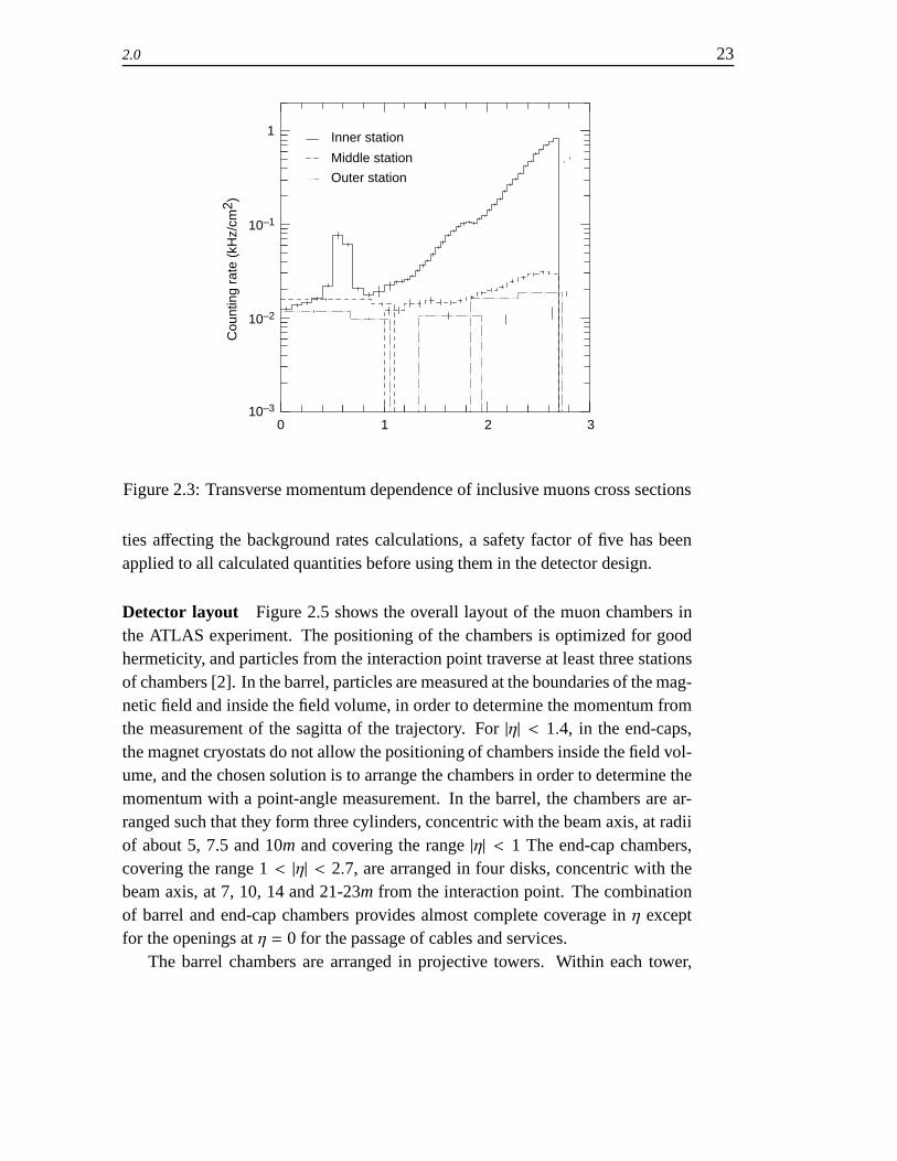
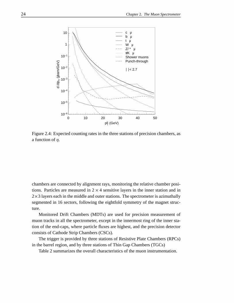
Figures 2.4 and 2.3 show the inclusive muons cross sections as a functionof transverse momentum and the expected counting rate in the three stationsof precision chambers respectively, calculated at the nominal LHC luminosityL=1034cm−2s−1. These results, combined with occupancy considerations, guidedthe choice of precision chambers granularities. Due to the significant uncertain-
2.0 23
1
10–1
10–2
10–3
0 1 2 3
Cou
ntin
g ra
te (
kHz/
cm2 )
Middle station
Outer station
Inner station
Figure 2.3: Transverse momentum dependence of inclusive muons cross sections
ties affecting the background rates calculations, a safety factor of five has beenapplied to all calculated quantities before using them in the detector design.
Detector layout Figure 2.5 shows the overall layout of the muon chambers inthe ATLAS experiment. The positioning of the chambers is optimized for goodhermeticity, and particles from the interaction point traverse at least three stationsof chambers [2]. In the barrel, particles are measured at the boundaries of the mag-netic field and inside the field volume, in order to determine the momentum fromthe measurement of the sagitta of the trajectory. For |η| < 1.4, in the end-caps,the magnet cryostats do not allow the positioning of chambers inside the field vol-ume, and the chosen solution is to arrange the chambers in order to determine themomentum with a point-angle measurement. In the barrel, the chambers are ar-ranged such that they form three cylinders, concentric with the beam axis, at radiiof about 5, 7.5 and 10m and covering the range |η| < 1 The end-cap chambers,covering the range 1 < |η| < 2.7, are arranged in four disks, concentric with thebeam axis, at 7, 10, 14 and 21-23m from the interaction point. The combinationof barrel and end-cap chambers provides almost complete coverage in η exceptfor the openings at η = 0 for the passage of cables and services.
The barrel chambers are arranged in projective towers. Within each tower,
24 Chapter 2. The Muon Spectrometer
c µ b µ t µ W µ Z/* µ π/K µ Shower muons Punch-through || < 2.7
10–6
10–5
10–4
10–3
10–2
10–1
1
10
d/d
p T (
µbar
n/G
eV)
pT (GeV)µ0 10 20 30 40 50
Figure 2.4: Expected counting rates in the three stations of precision chambers, asa function of η.
chambers are connected by alignment rays, monitoring the relative chamber posi-tions. Particles are measured in 2 × 4 sensitive layers in the inner station and in2×3 layers each in the middle and outer stations. The spectrometer is azimuthallysegmented in 16 sectors, following the eightfold symmetry of the magnet struc-ture.
Monitored Drift Chambers (MDTs) are used for precision measurement ofmuon tracks in all the spectrometer, except in the innermost ring of the inner sta-tion of the end-caps, where particle fluxes are highest, and the precision detectorconsists of Cathode Strip Chambers (CSCs).
The trigger is provided by three stations of Resistive Plate Chambers (RPCs)in the barrel region, and by three stations of Thin Gap Chambers (TGCs)
Table 2 summarizes the overall characteristics of the muon instrumentation.

2.1 25
chamberschambers
chambers
chambers
Cathode stripResistive plate
Thin gap
Monitored drift tube
Figure 2.5: Three-dimensional view of the muon spectrometer chambers layout.
2.1 Precision chambers
The muon spectrometer has been designed to allow momentum measurementswith a precision ∆pT/pT < 10−4 × p/GeV for pT>300 GeV. At lower energies,the resolution is limited to a few percent by multiple scattering and by energyloss fluctuation in the calorimeters. Being necessary to obtain such a precisionby means of three-point measurements, each point need to be measured with anaccuracy better than 50µm. In addition to this requirement, chamber design mustguarantee stability of operation for the entire lifetime of the ATLAS experiment,also considering the irradiated environment. Moreover, the total surface to becovered (∼ 5000m2) calls for particular attention to the price of the technologiesto be used.
Every muon track coming from the interaction point is measured at least bythree stations. Precision measurements are made along the bending direction ofthe magnetic field by MDTs in all the spectrometer except in the first station inthe end-cap and for η > 2, where the rate and background conditions guided the

26 Chapter 2. The Muon Spectrometer
Precision Chambers Trigger Chambers
CSC MDT RPC TGCNumber of chambers 32 1194 596 192Number of readout channels 67000 370000 355000 440000Area covered (m2) 27 5500 3650 2900
Table 2.1: Overview of the muon chamber instrumentation
Longitudinal beam
In-plane alignment
Multilayer
Cross plate
Figure 2.6: Schematic diagram of an MDT.
choice of CSCs.
2.1.1 Monitored Drift Chambers
MDT chambers are made of aluminum tubes of 30mm diameter and 400µmwall thickness, with a central 50µm diameter W-Re wire [4] [5]. The tubes arearranged in 2 × 4 monolayers for the inner stations and 2 × 3 monolayers for themedium and outer stations. A schematical view of the structure of an ATLASMDT is shown in figure 2.6. This design allows to improve the single-wire pre-cision and provides the necessary redundancy for track reconstruction. The twomultilayers of each station are placed on either side of a special support structure(spacer), providing accurate positioning of the tubes with respect to each other.The support structure also slightly bends the tubes of the chambers which are not
2.1 27
Anode wires
Cathode strips
d
d
WS
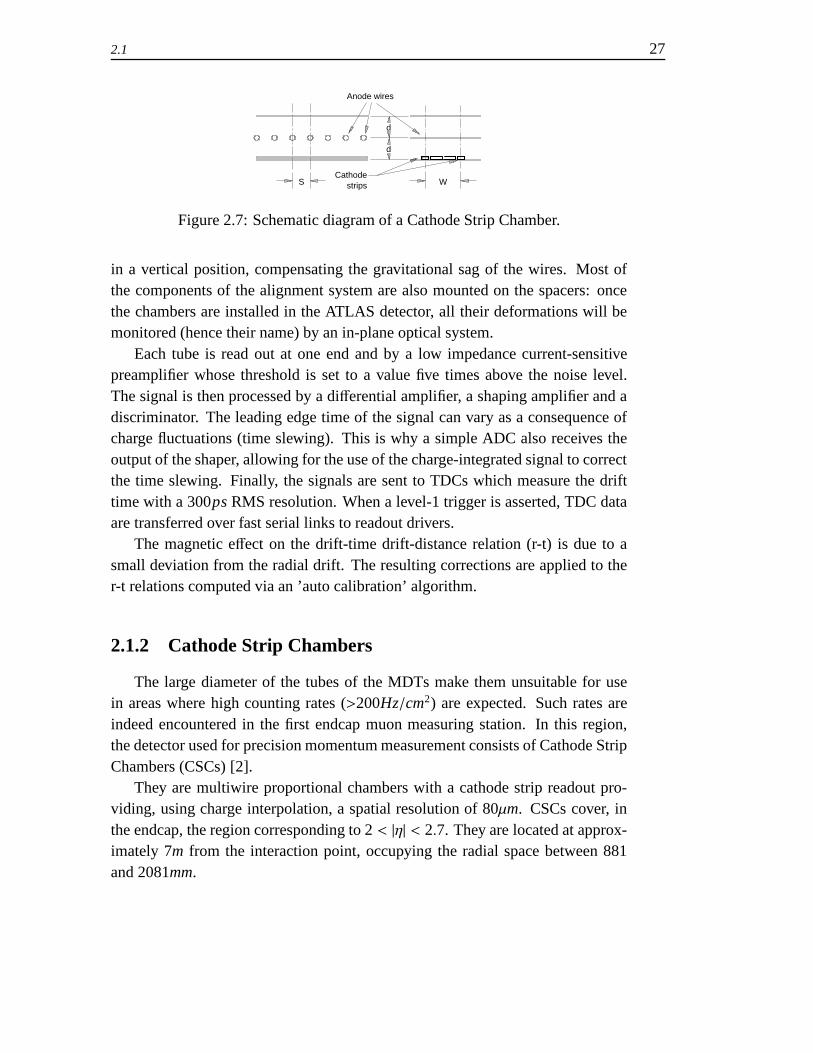
Figure 2.7: Schematic diagram of a Cathode Strip Chamber.
in a vertical position, compensating the gravitational sag of the wires. Most ofthe components of the alignment system are also mounted on the spacers: oncethe chambers are installed in the ATLAS detector, all their deformations will bemonitored (hence their name) by an in-plane optical system.
Each tube is read out at one end and by a low impedance current-sensitivepreamplifier whose threshold is set to a value five times above the noise level.The signal is then processed by a differential amplifier, a shaping amplifier and adiscriminator. The leading edge time of the signal can vary as a consequence ofcharge fluctuations (time slewing). This is why a simple ADC also receives theoutput of the shaper, allowing for the use of the charge-integrated signal to correctthe time slewing. Finally, the signals are sent to TDCs which measure the drifttime with a 300ps RMS resolution. When a level-1 trigger is asserted, TDC dataare transferred over fast serial links to readout drivers.
The magnetic effect on the drift-time drift-distance relation (r-t) is due to asmall deviation from the radial drift. The resulting corrections are applied to ther-t relations computed via an ’auto calibration’ algorithm.
2.1.2 Cathode Strip Chambers
The large diameter of the tubes of the MDTs make them unsuitable for usein areas where high counting rates (>200Hz/cm2) are expected. Such rates areindeed encountered in the first endcap muon measuring station. In this region,the detector used for precision momentum measurement consists of Cathode StripChambers (CSCs) [2].
They are multiwire proportional chambers with a cathode strip readout pro-viding, using charge interpolation, a spatial resolution of 80µm. CSCs cover, inthe endcap, the region corresponding to 2 < |η| < 2.7. They are located at approx-imately 7m from the interaction point, occupying the radial space between 881and 2081mm.

28 Chapter 2. The Muon Spectrometer
Figure 2.7 shows a schematic view of a CSC. The anode-cathode spacing d isequal to the anode wire pitch S , which has been fixed at 2.54mm. The cathodereadout pitch W is 5.08mm. In a typical multiwire proportional chamber signalson the anode wires are read out, thus limiting the spatial resolution to S/
√12. In
a CSCs a higher precision can be achieved measuring the charge induced on thesegmented cathode by the avalanche formed on the anode wire.
2.2 Trigger Chambers
The three main requirements of the muon spectrometer trigger system are:
• Bunch crossing identification. In order to correctly associate a trigger to abunch crossing, the trigger detectors must have a time resolution better thanthe LHC bunch spacing of 25ns.
• pT thresholds. The need for well defined pT cut-offs in moderate magneticfields, calls for a granularity of the order of 1cm.
• Second coordinate measurement. The trigger chambers must provide themeasurement of the coordinate orthogonal to the one measured in the pre-cision chambers, with a typical resolution of 5-10mm.
To fulfill these requirements optimizing also the total cost of the system, it hasbeen chosen to use two different technologies: Resistive Plate Chambers in thebarrel and Thin Gap Chambers in the endcaps.
2.2.1 Thin Gap Chambers
The structure of Thin Gap Chambers (TGCs) is very similar to the one ofmultiwire proportional chambers, with the difference that the anode-to-anode dis-tance is larger than the anode-cathode one. Figure 2.8 shows the inner struc-ture of a TGC. When operated with a highly quenching gas mixture (CO2:n-C5H12=55%:45%), this chambers work in a saturated mode, thus allowing forsmall sensitivity to mechanical deformations, which is very important for such alarge detector as ATLAS [6].
The saturated mode also has two more advantages:
• the signal produced by a minimum ionizing particle has only a small depen-dence on the incident angle up to angles of 40 degrees;

2.3 29
1.8 mm
1.4 mm
1.6 mm G-10
50 µm wire
Pick-up strip
+HV
Graphite layer
Figure 2.8: Structure of a TGC.
• the tails of the pulse-height distribution contain only a small fraction of thepulse-heights (less than 2%). In particular the response to slow neutrons issimilar to that of minimum ionizing particles. No streamers are observed inany operating conditions.
TGCs provide two functions in the endcap: muon trigger and azimuthal coor-dinate measurement. The middle tracking station of MDTs is equipped with sevenlayers (one triplet and two doublets) of TGCs, providing both functionalities. Theinner tracking layer of precision chambers is equipped with two layers of TGCs,providing only the second coordinate measurement. The second coordinate in theouter precision station is obtained by extrapolation from the middle station. Theradial (bending) direction is measured by reading which wire-group is hit; the az-imuthal coordinate is obtained from the radial strips.
Since the TGCs are located outside the endcap magnetic field and they canuse only a small lever arm (∼1m), they need a fine granularity also in the bendingdirection. To obtain the required momentum resolution it has been chosen to varythe number of wires in a wire-group as a function of η, from 4 to 20 wires, i.e.from 7.2 to 36mm. The alignment of the wire groups in two consecutive layers isstaggered by half the group width.
The 3698 chambers (corresponding to a total wire area of 6200m2) are mountedin two concentric rings on each endcap: an external one called outer or endcap(1.05 < η < 1.6) and an internal one, called inner or forward (1.6 < η < 2.4).The forward ring is divided in two logically independent rings at η = 2. In orderto cope with the higher background rate expected in the innermost rings, threedifferent trigger thresholds can be set for the three rapidity regions.

30 Chapter 2. The Muon Spectrometer
transverse-momentum cuts
DAQDAQInformation on hit strips Information on hit strips & wire groups
and on multiplicitiesMultiplicity for differentROI information
On detector
Off detector
Information on muon candidates
LVL2 DAQCTP
2 candidates per sectorPt thresholds for max.
TGC-detector
FE electronics
64 sectors
FE electronics
RPC-detector
TGC trigger/ read-out
hit pattern
144 sectors
CHS01aV01
RPC trigger/ read-out
Muon to CTP
interface
Figure 2.9: Block diagram of the level-1 muon trigger system.
2.3 The level-1 muon trigger
The information provided by the trigger chambers (RPCs and TGCs) is usedby a dedicated Muon Trigger System to decide whether muons above a giventhreshold were produced in a certain event. The sharpness of the pT cut appliedby the trigger is mainly given by the information read out from the detectors inthe bending projection. However, the information in the non-bending view helpsto reduce the background trigger rate from noise hits in the chambers producedby low-energy photons, neutrons and charged particles, as well as localizing thetrack candidates in space as required for the LVL2 trigger. In addition, the trig-ger chamber information in the non-bending view provides the second coordinatemeasurement for offline reconstruction of muons (the precision chambers give in-formation only in the bending projection).
The basic principle of the algorithm is to require a coincidence of hits in thedifferent chamber layers within a road. The width of the road is related to the pT
threshold to be applied. Space coincidences are required in both views, with atime gate close to the bunch-crossing period (25ns). Figure 2.9 shows the block

2.3 31
diagram of the level-1 muon trigger system.The level-1 muon trigger has to provide to the Central Trigger Processor the
multiplicity of muon candidates for each of the six pT thresholds. This is im-portant so that, for example, a low-pT di-muon trigger can be maintained at highluminosity. It is foreseen that the threshold on the di-muon trigger will be keptat about 6GeV per muon for L = 1034cm−2s−1, while the threshold for the single-muon trigger will have to be about 20GeV for an acceptable trigger rate. Giventhe steeply falling muon pT distribution, it is important that muons should onlyvery rarely be double counted (e.g. in areas of overlapping chambers), giving fakedi-muon triggers from single-muon events. It is therefore required by design thatat most 10% of the di-muon triggers shall be due to doubly-counted single muons.A detailed description of the working principles and performance of the ATLASdi-muon trigger will be presented in chapter 7.

Chapter 3
The Resistive Plate Chambers
The first publication on Resistive Plate Chambers was in 1981 [8]. In thefollowing years they had great development and now they are widely used in bothhigh-energy and astro-particle physics.
3.1 Detector description
RPC operation is based on the detection of the gas ionization produced bycharged particles when traversing the active area of the detector, under a stronguniform electric field applied using resistive electrodes. The electrodes are madeof a mixture of phenolic resins (usually called bakelite), which has a volume re-sistivity ρv between 109 and 1012Ωcm. Glass can be used as plate material as well,and the plates are kept spaced by insulating spacers. The thickness of the platesand the distance at which they are kept are different for different experiments.Here and in the following we refer to the characteristics of RPCs for the ATLASexperiment.
RPCs used in the ATLAS experiment have 2mm thick plates, kept at 2mm onefrom each other. The spacers are cylindrical with 12mm diameter and are placedone every ∼10cm in both directions. The external plate surfaces are coated by thinlayers of graphite painting. The graphite has a surface resistivity of ∼ 100kΩ,thus allowing uniform distribution of the high voltage along the plates without cre-ating any Faraday cage that would prevent signal induction outside the plates (aswould happen using, for example, metallic electrodes). Between the two graphitecoatings is applied a high voltage of about 10kV , resulting in a very strong electricfield (∼ 5MV/m) which provides avalanche multiplication of the primary electrons
32
3.2 33
generated by ionization by the incident particle. The presence of such a high elec-tric field calls for extreme smoothness of the inner surfaces of the bakelite plateswhich is obtained covering the surfaces with a thin layer of linseed oil. The dis-charge electrons drift in the gas and the signal induced on pick-up copper strips isread-out via capacitive coupling, and processed by the front-end electronics.
3.2 Avalanche growth and signal detection
In RPCs the electrons generated by primary ionization are subjected to thestrong electric field which make them drift towards the anode. Along their paththey collide with other electrons in the medium. Between two consecutive colli-sions, an electron may increase its kinetic energy enough to generate a secondaryionization, thus starting an exponential multiplication. The mean free path ofelectrons in the medium is λ = 1/α, where α is called the first Townsend coeffi-cient. Defining n the number of electrons drifting in the gas at a given time, theincrement dn obtained during the drift for a distance dx is
dn = ndxλ= nαdx.
Integrating over a path x, the total number of electrons is
N = n0 eαx = n0 eαvd t
where vd is the drift velocity of electrons in the gas, depending on the gasmixture and on the electric field. Assuming the electric field uniform during theavalanche growth, implies a constant first Townsend coefficient. This is not truewhen the spatial charge density of the avalanche is large enough to cause distor-tions on the field generated by the plates. In this conditions α has a dependenceon x and the exponential has to be substituted by an integral over x in the previousexpressions.
When the avalanche reaches an electron multiplicity of ∼ 106 electrons, itsgrowth slows down due to space charge effects, entering the so called saturatedregime [23]. For extremely high values of the electronic charge (established byMeek in ∼ 108 electrons for noble gases) the avalanche becomes the precursorof a new process called streamer. This is a plasma filament between the elec-trodes which produces an extremely high current in the gas (∼ 100 times largerthan the typical avalanche). The streamer does not evolve in a spark because of
34 Chapter 3. The Resistive Plate Chambers
the electrodes resistivity, and it is prevented to propagate transversely an oppor-tune photon quencher in the gas mixture. Streamer signals are therefore greaterand easier to detect, but also longer in time and with a higher charge per count.In particular this last characteristic limits the rate capability of the detector oper-ated in streamer mode to a few hundred of Hzcm−2. Adopting gas mixtures basedon electronegative components allows to retard the appearance of the streamer interms of the applied electric field [11][12][13]. Finally, the introduction of S F6 asa quencher removed completely the problem of the streamer, allowing to work ina pure avalanche mode [9].
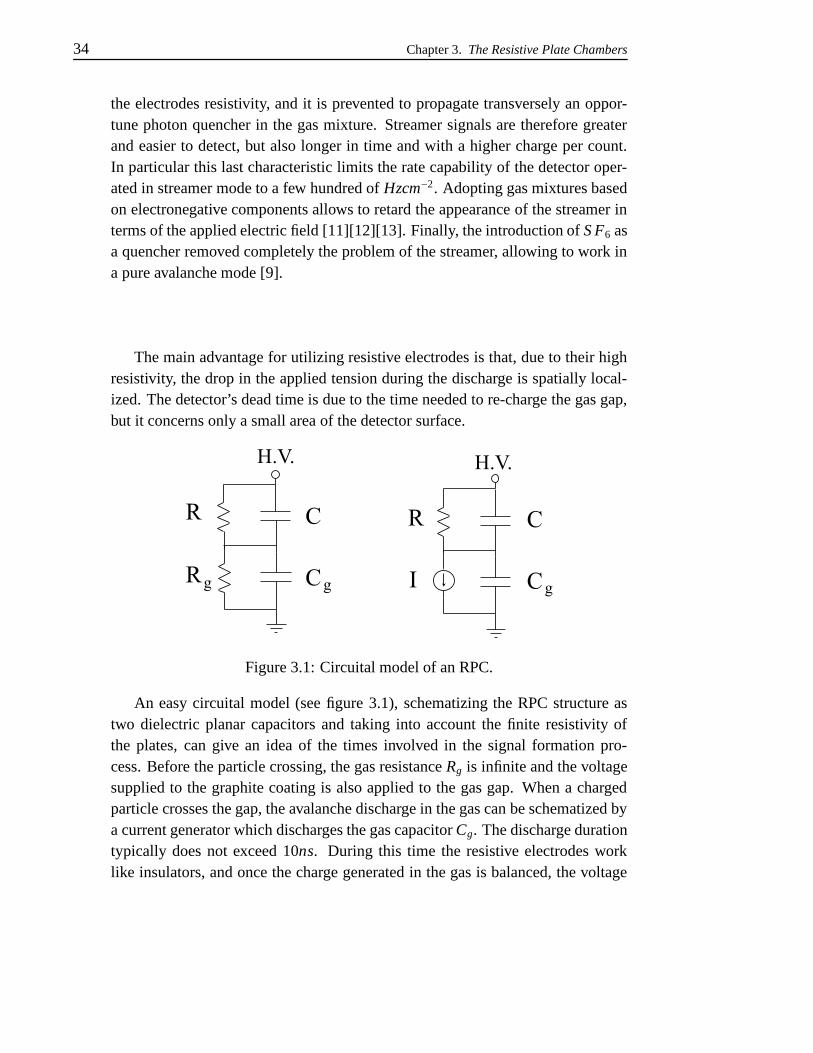
The main advantage for utilizing resistive electrodes is that, due to their highresistivity, the drop in the applied tension during the discharge is spatially local-ized. The detector’s dead time is due to the time needed to re-charge the gas gap,but it concerns only a small area of the detector surface.
Figure 3.1: Circuital model of an RPC.
An easy circuital model (see figure 3.1), schematizing the RPC structure astwo dielectric planar capacitors and taking into account the finite resistivity ofthe plates, can give an idea of the times involved in the signal formation pro-cess. Before the particle crossing, the gas resistance Rg is infinite and the voltagesupplied to the graphite coating is also applied to the gas gap. When a chargedparticle crosses the gap, the avalanche discharge in the gas can be schematized bya current generator which discharges the gas capacitor Cg. The discharge durationtypically does not exceed 10ns. During this time the resistive electrodes worklike insulators, and once the charge generated in the gas is balanced, the voltage

3.2 35
applied to the gas gap is null. Then the system goes back to the initial conditiondischarging the electrodes capacitor:
dqC
qC= −
dtR(C + Cg)
with a characteristic time τ which can be expressed as
τ = ρ2Sd
(
εS2d+ε0S
g
)
= ρε0
(
εr +2dg
)
being d the plate thickness, g the gap thickness,and ρ and εr the resistivityand the dielectric constant of the bakelite respectively. A typical value for τ is∼ 10ms, which is orders of magnitude greater than the signal duration (∼ 10ns),and represents the dead time of the detector. It is to be noted that this dead time isindeed limited just to a small area of the detector.
The pick-up strips behave as signal transmission lines of well defined impedanceand allow to transmit the signals at large distance with minimal loss of amplitudeand time infinformationtrips are usually terminated at one end with by front-endelectronics and on the other one by proper resistor to avoid reflections. The in-duced charge is split in two parts, thus reducing the readable signal by one half.The read-out electrode can be described as a current generator charging a paral-lel RC circuit. The resistor R connecting the line to the ground is half the lineimpedance. The electrode capacity C is proportional to the pick-up area deter-mined by the spatial distribution spread of the induced charge. The time constantτ = RC for typical values of these parameters is of the order of tenths of ps, muchshorter than the rise time of the signal: the current injected in the strip is at anytime proportional to the current of the discharge in the gap.
Assuming the ionization electrons uniformly distributed along the gap depth,n is defined to be the number of ionization electrons per unit length. At a time tall the primary clusters produced at a distance x > vt, being v the drift velocity,were absorbed, while all the others had a gain ∼ eαvt. In RPCs the ion current isessentially invisible and only electrons give a prompt signal. The total number ofelectrons in motion in the gap at the time t is
N (t) = n (g − vt) eαvt

36 Chapter 3. The Resistive Plate Chambers
thus inducing a current on the pick-up electrodes given by
i (t) = eN (t)vg= evn
(
1 −vtg
)
eαvt
The prompt charge q is given by the current integral up to the maximum drifttime tmax = g/v [14]
q =∫ g/v
0i (t) dt ≈ eng
(αg)2eαg
to be compared with the total charge Q flown in the gap
Q =∫ g
0eneαxdx ≈
engαg
eαg
The distance between the gas gap and the read-out electrodes is increased bythe thickness d of the resistive plates. A simple calculation in which the platesand the gas gap are treated as three serially connected capacitors leads to onemore correction factor on q, giving a total ratio of
qprompt
Q=
1αg
[
1 +2dεrg
]
12
which takes into account also the splitting of the induced signal between thefront-end and the terminating resistor.
3.3 The gas mixture
The gas mixture is crucial in the RPC operation and it must be carefully chosenin order to obtain the required performances. The first consideration to do whenchoosing a gas mixture for RPCs is whether the detector will work in avalancheor streamer mode.
The filling gas is usually composed by an optimized mixture. To operate thechamber in streamer mode, the gas should provide a robust first ionization and alarge avalanche multiplication even at low applied field. One typical choice is Ar-gon, which, providing great avalanche increase with abundance of electrons, setsthe ideal condition for the streamer production. If the desired operating regime isavalanche mode, the main component should be an electro-negative gas with highenough primary ionization, but with a low mean free path for electron capture, inorder to maintain the number of electrons in an avalanche below the Meek limit.

3.4 37
A gas showing this characteristics is, for example, C2H2F4.The gas mixtures used for RPC operation often contain one more component,
with the role of absorbing the photons produced by electron-ion recombinations,thus avoiding photoionization (with related multiplication) and limiting the lat-eral charge spread. Typically an hydrocarbon shows the characteristics describedabove.
Significant changes in environmental variables, such as temperature and pres-sure, alter the characteristics and properties of the filling gas (for example thedensity ρ), and influence the ionization and multiplication processes. This is thereason why performances at the same applied field but with different environmen-tal conditions are in general different. In order to make meaningful comparisonbetween data sets taken at some distance in time one from another, the appliedvoltage value are normalized according to the formula
HVe f f = HVT 1,P1
app
T 1
T 0
P0
P1
justified with the hypothesis that the gas discharge related phenomena are in-variant for any change in P,V,T which leaves the ratio of the voltage over the gasdensity unchanged.
3.4 RPC working regimes and performances
RPCs are operated in avalanche or streamer mode [10], corresponding to thetwo different discharge mechanisms described in 3.2. Typical signal amplitudefor an avalanche is ∼ 1mV , with a duration of about 4ns and an average chargeof ∼ 1pC. The amplitude of signals induced by streamers is typically ∼ 100mV ,while their duration is of the order of 10 to 20ns, producing a ∼ 100pC charge.
Avalanche signals need a strong amplification and have high frequency com-ponents due to their very short duration, and are therefore particularly difficult todetect. Streamer signals on the contrary do not need any complex signal process-ing.
When a streamer occurs, both the charge and the detector surface involvedin the discharge are larger compared to the ones associated to an avalanche. Asdiscussed in 3.2, this implies a lower rate capability of the detector. Typical ratecapabilities for RPCs working in streamer mode are of the order of 100Hz/cm2.This value can be increased reducing the charge released in the gas, i.e. workingin avalanche mode, or decreasing the plate resistivity.

38 Chapter 3. The Resistive Plate Chambers
By carefully choosing the gas mixture it is possible to obtain a stable avalancheworking mode, with a large operating voltage plateau not contaminated by stream-ers. A sophisticated read-out electronic allows to detect the small and fast signalsgenerated by avalanches, thus reaching rates capabilities up to 1kHz/cm2.
Avalanche operation is also safer for what concerns the detector ageing effects,which depend on the total integrated charge.
RPCs spatial resolution depends both on the read-out geometry an electronics.Using an analog readout it is possible to obtain resolution of ∼ 1cm, but with adigital read-out the resolution is limited by the strip width, typically of the orderof a few centimeters.
Concerning time resolution, it is natural to compare RPCs with wire detec-tors. The drift times in the radial electric field are different for different clusters,depending on their distance from the wire. The signal duration can be as long ashundreds of ns and is fixed by the cluster at maximum distance from the wire.On the contrary, the high and uniform electric field applied to the gas gap by theelectrodes is the same for all primary clusters, producing at fixed time the samegrowth, limited by the distance of the primary clusters from the anode. The sig-nal at any time is the sum of simultaneous contributions from all primary clustersmultiplications. The resulting time jitter for detectable signals is always < 2ns.
Chapter 4
Ageing test of ATLAS RPCs atX5-GIF
The accelerator background at LHC will be dominated by soft neutrons andgammas that are generated by beam protons at very small angle [15]. Such aheavy background calls for severe requirements on the trigger detector in termsof rate capability and time resolution, crucial for bunch crossing identification.Moreover, almost for all the chambers installed in the ATLAS cavern, it will beimpossible to perform any hardware reparation or substitution once the detectoris installed. It is therefore crucial that the chambers do not show any abnormalageing effect which could degrade their performace during the ∼10 years of theATLAS operation.
For this reason an ageing test of three production ATLAS BML RPCs hasbeen performed at CERN. The chambers have been irradiated with photons froma 137Cs source in order to test their rate capability and to integrate a total chargeper cm2 corresponding to ∼ 10 ATLAS years including the safety factor of 5,which is applied in the requirements placed on all the ATLAS detectors to takeinto account the uncertainties in the background rate.
In the following, we will refer to ATLAS years as a measurement of the ageingof the detector. One ATLAS year corresponds to a charge of 30mC/cm2, which isobtained assuming 109 counts per year per cm2 and an average charge per countof 30pC. This calculation includes the abovementioned safety factor of 5.
39

40 Chapter 4. Ageing test of ATLAS RPCs at X5-GIF
4.1 The X5 beam
The X5 beam is part of the West Area test beam complex at CERN. It can workas a secondary or tertiary particle beam, providing hadrons, electrons or muons ofenergy between 10 and 250 GeV .
A 450GeV/c primary proton beam, with typical intensities of 2 × 10¹² protonsper bunch, is extracted from the SPS and directed on the primary target, fromwhich a secondary beam is extracted.
The secondary beam is called H3 and normally consists mainly of pions andelectrons, whose energy and polarity may change according to the requirementsof the West Area users, ranging normally around 120GeV/c up to a maximum of250GeV/c.
The H3 beam is split into two branches, each transporting about 107 particlesper SPS cycle to the X5 and X7 secondary targets. The average decay length
Figure 4.1: X5 Beam from SPS.
of charged pions is ∼ 55m/GeV . For example at 120 GeV/c the average decaylength is about 6600m. Over a length of 100m between the splitter and the first X5bending, some 1.5% of the pions decay as π −→ µ + ν. According to the averagepion intensity more than 105µ± are produced. The pion decay kinematics impliesthat 0.57 ≤ pµ/pπ ≤ 1.0. The X5 beam will transport these muons if its settingsare tuned to momenta in the appropriate range. Muons will always have 80± 20%of the H3 momentum.
A common situation for tracking tests is a high momentum tertiary beam withpX5 well above 57% of the H3 momentum (figure 4.1).
In this case typically some 104 muons per burst are contained within an area of10 × 10 cm2. The remaining muons are widely spread over several square metres.
4.2 41
4.2 The Gamma Irradiation Facility
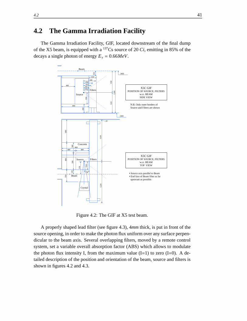
The Gamma Irradiation Facility, GIF, located downstream of the final dumpof the X5 beam, is equipped with a 137Cs source of 20 Ci, emitting in 85% of thedecays a single photon of energy Eγ = 0.66MeV .
Beam
150
224
340250205
160150
Source
Filters
40035
0
800
260
680
800400 400
300
800
500
Beam
120
Source
370 25
0
350
Crystal 1220
1220
10
2400
610
1260
650
3660
X5C GIFPOSITION OF SOURCE, FILTERS
w.r.t. BEAMSIDE VIEW
N.B. Only outer borders of Source and Filters are shown
X5C GIFPOSITION OF SOURCE, FILTERS
w.r.t. BEAMTOP VIEW
Source axis parallel to Beam End face of Beam filter as far upstream as possible.
Concrete
Filters
150
Figure 4.2: The GIF at X5 test beam.
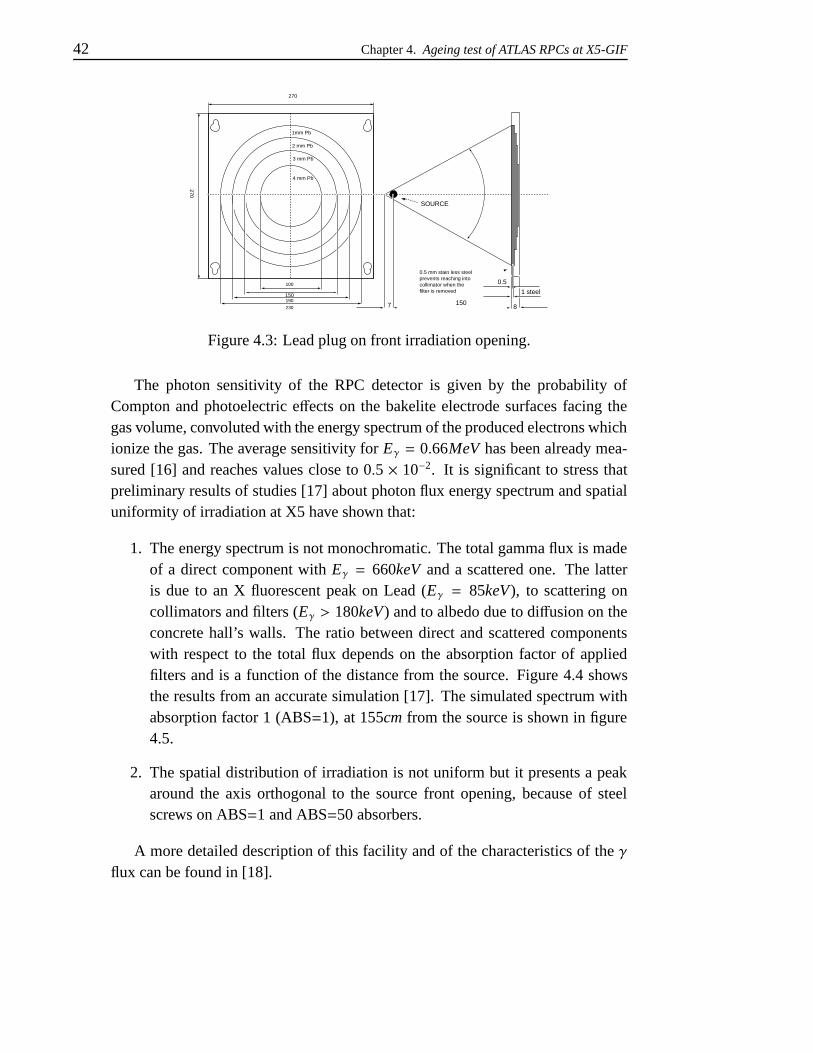
A properly shaped lead filter (see figure 4.3), 4mm thick, is put in front of thesource opening, in order to make the photon flux uniform over any surface perpen-dicular to the beam axis. Several overlapping filters, moved by a remote controlsystem, set a variable overall absorption factor (ABS) which allows to modulatethe photon flux intensity I, from the maximum value (I=1) to zero (I=0). A de-tailed description of the position and orientation of the beam, source and filters isshown in figures 4.2 and 4.3.
42 Chapter 4. Ageing test of ATLAS RPCs at X5-GIF
SOURCE
0.5
1 steel
81507230
100
190150
270
270
1mm Pb
2 mm Pb
3 mm Pb
4 mm Pb
0.5 mm stain less steelprevents reaching intocollimator when thefilter is removed
Figure 4.3: Lead plug on front irradiation opening.
The photon sensitivity of the RPC detector is given by the probability ofCompton and photoelectric effects on the bakelite electrode surfaces facing thegas volume, convoluted with the energy spectrum of the produced electrons whichionize the gas. The average sensitivity for Eγ = 0.66MeV has been already mea-sured [16] and reaches values close to 0.5 × 10⁻². It is significant to stress thatpreliminary results of studies [17] about photon flux energy spectrum and spatialuniformity of irradiation at X5 have shown that:
1. The energy spectrum is not monochromatic. The total gamma flux is madeof a direct component with Eγ = 660keV and a scattered one. The latteris due to an X fluorescent peak on Lead (Eγ = 85keV), to scattering oncollimators and filters (Eγ > 180keV) and to albedo due to diffusion on theconcrete hall’s walls. The ratio between direct and scattered componentswith respect to the total flux depends on the absorption factor of appliedfilters and is a function of the distance from the source. Figure 4.4 showsthe results from an accurate simulation [17]. The simulated spectrum withabsorption factor 1 (ABS=1), at 155cm from the source is shown in figure4.5.
2. The spatial distribution of irradiation is not uniform but it presents a peakaround the axis orthogonal to the source front opening, because of steelscrews on ABS=1 and ABS=50 absorbers.
A more detailed description of this facility and of the characteristics of the γflux can be found in [18].

4.3 43
Figure 4.4: Simulated photon flux components as a function of the distance fromthe source.
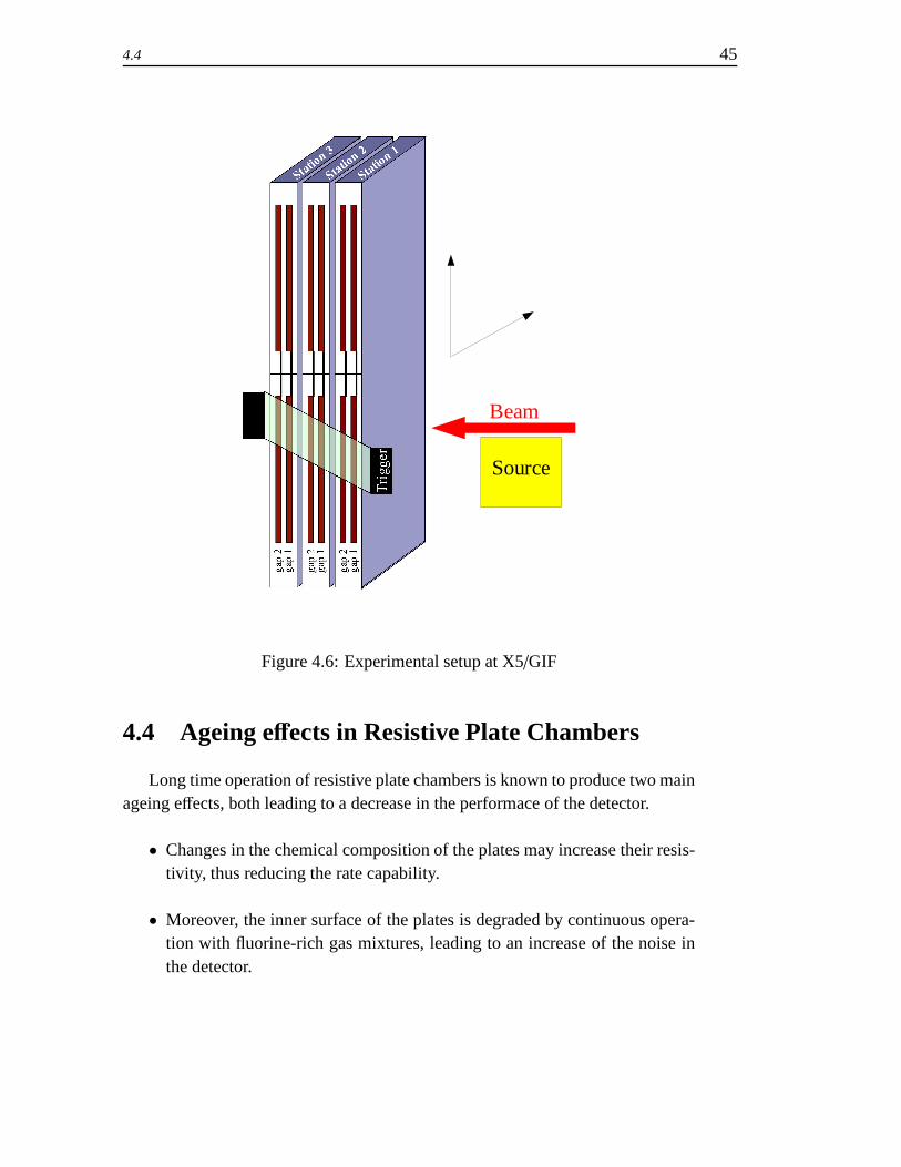
4.3 Experimental setup
Three production ATLAS RPC chambers (BML-D) are installed in the GIFarea, along the beam line. A schematical view and a picture of the setup areshown in figures 4.6 and 4.7 respectively. The chambers have 2 detector layerswhich are read out by strips oriented in both the η and ϕ directions. The chambersare perpendicular to the beam line, with the long side (about 4m) oriented in thevertical direction. For details on the chamber structure, see [2]. The chambers areoperated with the ATLAS gas mixture C2H2F4/i–C4H10/S F6 = 94.7/5/0.3.
The trigger is provided by the coincidence of three scintillator layers of 33x40cm2, each made of three slabs. During the beam runs, the three layers are alignedalong the beam line, while for the cosmic rays runs, they are arranged as a tele-scope with the axis oriented at 40 degrees with respect to the vertical direction, inorder to maximize the trigger rate.Signals from the frontend electronics are sent to a standard ATLAS “splitter board”[7] as in the final architecture foreseen for the trigger and readout electronics, and

44 Chapter 4. Ageing test of ATLAS RPCs at X5-GIF
0
50
100
150
200
x 10 4
0 0.2 0.4 0.6
Pb X fluorescence
Compton on walls
Compton on filters and collimators
Photon Energy [MeV]
ABS 1 155 cm
Ph
oton
Flu
x [c
m-2
s-1M
eV-1
]
Figure 4.5: Simulated spectrum of the scattered photons at 155 cm from the sourceon the axis of the irradiation field and for absorption factor (ABS) 1. The threemain contributions are indicated: two are from filters and collimators (white area),the other from walls and floor (dashed area). The total flux of scattered pho-tons amounts to 6.4×105cm−2s−1, while the flux of direct photons (at 662keV , notshown) is 8.0×105cm−2s−1 [18].
subsequently to TDCs working in common stop mode (see [19]) which record upto 16 hits per event per channel, in a 2µs gate. Both the leading and falling edgesof the signals are recorded. The data acquisition is performed using a LabViewTM
application.
The DCS system, also implemented using LabViewTM, records both the lowand and high voltages as well as the gap currents. Gas composition, togetherwith all relevant environmental data such as pressure, temperature and relativehumidity are controlled as well. The gas relative humidity, also monitored by theDCS, is set in the range of 30%-50% by bubbling in water a fraction of the totalgas flux.
4.4 45
Source
Beam
Figure 4.6: Experimental setup at X5/GIF
4.4 Ageing effects in Resistive Plate Chambers
Long time operation of resistive plate chambers is known to produce two mainageing effects, both leading to a decrease in the performace of the detector.
• Changes in the chemical composition of the plates may increase their resis-tivity, thus reducing the rate capability.
• Moreover, the inner surface of the plates is degraded by continuous opera-tion with fluorine-rich gas mixtures, leading to an increase of the noise inthe detector.

46 Chapter 4. Ageing test of ATLAS RPCs at X5-GIF
Figure 4.7: Experimental setup at X5/GIF. The chambers under test are visible inthe background, in their blue support structure. The orange box in the foregroundcontains the source, while the pink structure supports the lead filters.
Both these ageing effects have been extensively studied during this test, andseveral techniques have shown their effectiveness in reducing to an acceptablelevel all the losses in performace related to the detector ageing.
4.4 47
4.4.1 Plate resistivity increase
Systematic tests carried out, in the ATLAS framework, on RPCs of differentsizes operated in avalanche mode at high working currents [24], showed a de-crease of the rate capability at fixed voltage as the main long term ageing effect.This effect was demonstrated to be due to the increase of the electrodes resistance[21].
Though all RPCs for the LHC experiments are designed with very large safetymargins of rate capability, great efforts have been dedicated to the study of theelectrode conduction properties due to the very long time of operation foreseen.The electrode resistance increase is found to be due to two main components:
• a long term effect, consisting in a progressive increase of the anodic graphitecoating resistivity; the cathodic layer is almost unaffected [22];
• an increase of the laminate resistance which depends both on the total inte-grated charge and on environmental conditions such as the relative humidity.
In the test described in the following, particular attention has been dedicatedto the study of the second of these two effects.
It has long been known ([10]) that the electrical properties of the plastic lam-inate depend on the environment temperature and relative humidity. Materialssuch as phenolic-melaminic laminates have a negative temperature coefficient, i.e.their resistivity decreases for increasing temperature. Moreover, when the platesare exposed to dry air circulation, their resistivity gradually increases even by alarge factor. This effect is completely reversible once the sample is left at roomRH for a sufficient time.
On the other hand, plates kept under high current densities (hundreds of µA/m2)for long periods, also show a gradual increase in resistivity which is found to befaster when the plates are operated at lower RH values. This effect of the relativehumidity has been shown ([20]) to be selective, in the sense that its effect is muchmore effective if the humidification is performed on the anode side of each plate.
These observations suggest that both the gas mixture and the external envi-ronment need to be humidified in order to guarantee that the anodes of the twoelectrode plates are operated in the proper RH conditions. To achieve the nec-essary control on the external relative humidity, the area surrounding the threechambers under test has been delimited using PET foils. The air relative humiditynear the chambers is hence controlled by means of two humidifiers.

48 Chapter 4. Ageing test of ATLAS RPCs at X5-GIF
4.4.2 Plate surface damage
The quality of the inner surface of the plates is crucial for the operation ofRPCs, since any damage of the surfaces translates to a disuniformity of the electricfield, thus increasing the noise in the detector.
The gas mixture used in ATLAS RPC will contain a high fraction (∼ 95%)of C2H2F4. Long term operation of RPCs with gas mixtures based on fluorinecompounds is known to lead to damages to the internal surface of the chambers,due to the reaction of the linseed oil coating layer with fluorine ions producedin the gas during the discharges. A more detailed study of the F− production inRPCs will be presented in chapter 5.
In order to reduce this ageing effect, particular attention has to be given tocarefully tune the gas flow, which has to be high enough to ensure proper removalof F− ions from the detector. Given the number of gas gaps to be used in theATLAS detector, the necessary gas flow would be so high that it is not affordableto achieve it without a recirculation system. Such a system will filter the outputgas from the chambers and send it again in the gas gaps, together with a smallfraction of new gas. During the test described in this chapter, a prototype of sucha recirculation system has been used, and its effectiveness tested.
4.5 Measurement techniques
In order to monitor the performaces for the detector, three types of measure-ments were carried out all along the test:
• quantities such as chamber efficiency, average cluster size and single count-ing rate where monitored by means of an offline analysis program specifi-cally developed for this test;
• plate resistivity measurements;
• the noise level was measured using the DCS system, in particular measuringthe gap currents;
4.5.1 Offline analysis
During the test, the chamber efficiencies were monitored using cosmic raystriggered by the scintillators, while high statistics efficiency measurements were

4.5 49
made when the X5 muon beam was available.For each event, the muon trajectory is reconstructed.The scintillator slabs of the trigger system, of size 11x40cm2, would only allow
a very modest tracking, not sufficient to eliminate all accidental hits at very highcounting rate induced by the source. The tracking capability is therefore improvedusing the hits recorded by the RPCs, as described below:
1. hits recorded by the RPC under test are ignored in the tracking;
2. only hits registered in a time window of 25ns around the beam peak are con-sidered useful for the track reconstruction, in order to reduce the probabilityto use an accidental photon hit in the tracking;.
3. for each electronic channel (i.e. for each strip) a dead time of 50ns is appliedby the analysis algorithm, in order to avoid any double counting due, forexample, to after pulses;
4. tracks are reconstructed only for events showing a single cluster in at leastthree layers (out of the five available). This is useful to improve the qualityof the reconstructed track eliminating, for example, di-muon events.
5. a track in both the η and ϕ directions is required.
6. the layer is considered efficient if it shows a cluster aligned to the trackwithin ± 1 strip.
The steps described above are repeated for each gas gap. In the evaluation ofthe efficiency of each layer, dead strips are not taken into account, i.e. a trackcrossing a strip known to be dead will not be considered as an inefficiency of thelayer. In addition to the efficiency, average cluster sizes are measured for eachlayer.
Particular importance, in conjunction with the efficiency measurements, hasbeen given to single counting rate measurements. They are performed on the samedata sets used for efficiency measurement, taking into account only hits which arefound to be not in time with the beam. Figure 4.8 shows, as an example, the timespectrum for the ϕ layer of Station1, gap 1. The plot refers to a run taken at fullsource exposure: the time window used for rate measurements is shown.
Data sets were taken with different front end electronic thresholds, source in-tensities, and operating voltages. The plateaus shown in figure 4.9, for example,
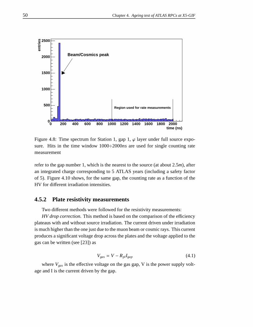
50 Chapter 4. Ageing test of ATLAS RPCs at X5-GIF
time (ns)0 200 400 600 800 1000 1200 1400 1600 1800 2000
entr
ies
0
500
1000
1500
2000
2500
Beam/Cosmics peak
Region used for rate measurements
Figure 4.8: Time spectrum for Station 1, gap 1, ϕ layer under full source expo-sure. Hits in the time window 1000÷2000ns are used for single counting ratemeasurement
refer to the gap number 1, which is the nearest to the source (at about 2.5m), afteran integrated charge corresponding to 5 ATLAS years (including a safety factorof 5). Figure 4.10 shows, for the same gap, the counting rate as a function of theHV for different irradiation intensities.
4.5.2 Plate resistivity measurements
Two different methods were followed for the resistivity measurements:HV drop correction. This method is based on the comparison of the efficiency
plateaus with and without source irradiation. The current driven under irradiationis much higher than the one just due to the muon beam or cosmic rays. This currentproduces a significant voltage drop across the plates and the voltage applied to thegas can be written (see [23]) as
Vgas = V − RplIgap (4.1)
where Vgas is the effective voltage on the gas gap, V is the power supply volt-age and I is the current driven by the gap.

4.5 51
HV (kV)8.5 9 9.5 10 10.5
HV (kV)8.5 9 9.5 10 10.5
effi
cien
cy
0
0.2
0.4
0.6
0.8
1
no source
a.f. 2
full source
Gap 1 -
Figure 4.9: Efficiency versus high voltage at different source intensities, as mea-sured with the muon X5 beam.The plot refers to Station 1, gap 1, ϕ, after 5 ATLASyears of ageing.
This drop causes the efficiency plateaus under irradiation to be shifted at higherHV values, as shown in figure 4.9. This shift allows to evaluate the plate resistivitywhen the gap current is also measured. Figure 4.11 shows an example of theapplication of this technique.
I-V characteristic in pure Argon. The standard ATLAS gas mixture is replacedby pure Ar. As shown in figure 4.12, the I-V curve is characterized in this case bya transition region around V=2kV with a fast current increase. For higher voltagesa linear current increase is observed. We assume that above the transition voltage,the drop across the Argon remains constant, so that the slope ∆V/∆I in the linearregion gives the plates total resistance.

52 Chapter 4. Ageing test of ATLAS RPCs at X5-GIF
HV (kV)8.5 9 9.5 10 10.5 11
HV (kV)8.5 9 9.5 10 10.5 11
)2ra
te (
Hz/
cm
-110
1
10
210
310
Gap 1 -
no source
a.f. 2
full source
Figure 4.10: Single rate measurement at different source intensities for Station 1,gap 1, η, after 5 ATLAS years of ageing.
4.5.3 Noise level monitoring
It is possible to evaluate the status of the inner surface of the plates usingthe single counting rate measurements described above. However, being the timebetween two consecutive data taking periods of the order of two months, it is nec-essary to use a monitoring tool providing more frequent noise level estimations.
One of the quantities continuously monitored by the DCS system for each gapis the gap current, defined as the total current driven by the gas, as read on a100kΩ resistance put on the ground connection of the gap (see figure 4.13). Itis a precise estimator of the number of avalanches in the gap and therefore, whenmeasured without source irradiation and without beam activity, of the noise level.
Gap current measurements as a function of the operating voltage where takenalmost daily all along the test.

4.6 53
0
0.2
0.4
0.6
0.8
1
1.2
8500 9000 9500 10000
Standard voltage (V)
Effic
ienc
y
No correction
No source
full source
0
0.2
0.4
0.6
0.8
1
1.2
8500 9000 9500 10000
Standard voltage (V)
Effic
ienc
y
After correction for resistivity
Figure 4.11: Procedure for plate resistivity measurement using efficiency plateaus.
4.6 Experimental results
4.6.1 Plate resistivity evolution
Figure 4.14 shows the evolution of the plate resistivity as a function of timefor the six gaps under test. The figure also shows the relative humidity of the gasmixture. Starting from October 2003 the environment surrounding the chamberswas put under a constant 50% RH value. The resulting decrease in resistivity isclearly visible in the plot. This effect was shown to be reversible: a short periodwithout humidification of the external air has indeed produced an increase in theplate resistivity, while once the external RH control was restored the resistivitiesof the gaps showed again a significant decrease.
It has to be noted that the resistivity values corresponding to the two measure-ment techniques are systematically different. This result is exactly what can beexpected considering that the Argon technique measures the average resistivityof the plates, using the whole surface of the electrodes for the measurement. Onthe other hand, the plateaus technique only measures the resistivity on a fractionof the detector surface, i.e. the one covered by the scintillator trigger. The gasinput to the chambers is on their bottom side, and the external air humidificationis provided by two humidifiers placed on the ground. This implies that the humid-ification is not constant along the plate surface; in particular, the lower parts of thegaps are better humidified, i.e. they have lower resistivity.

54 Chapter 4. Ageing test of ATLAS RPCs at X5-GIF
0
50
100
150
200
250
300
350
400
450
500
0 500 1000 1500 2000 2500 3000
Standard voltage (V)
Gap
cur
rent
(uA)
gap 1
gap 2
gap 3
gap 4
gap 5
gap 6
Figure 4.12: I-V characteristics in pure Argon.
Figure 4.13: Gap current measurement.

4.6 55
Resistivity evolution
0.00
50.00
100.00
150.00
200.00
250.00
300.00
350.00
400.00
450.00
01/09/2002 10/12/2002 20/03/2003 28/06/2003 06/10/2003 14/01/2004 23/04/2004 01/08/2004 09/11/2004 17/02/2005
(
G
cm)
@ 2
0°C
0
50
100
150
200
250
inte
gra
ted
ch
arg
e (m
C/c
m^
2)g
as R
H (
%)
gap 1 Ar gap 2 Ar gap 3 Ar gap 4 Ar gap 5 Argap 6 Ar gap 1 eff gap 2 eff gap 3 eff gap 4 effgap 4 eff gap 6 eff Ageing (mC/cm^2) gas RH
ext RH control ON OFF ON
Figure 4.14: Plate resistivity evolution.
4.6.2 Detector performance
Chamber efficiencies at closed source, measured periodically both with cos-mics rays and with the X5 beam, did not show any loss along the test.
Figure 4.9 shows the efficiency vs HV plot for Station 1 gap 1 ϕ at differentsource intensities. The high current driven by the gaps under source irradiationcauses a voltage drop across the plates. Due to this drop, the plateaus show a shifttowards higher voltages an a slower raise, compared with the plateaus taken with-out irradiation. This effect is enhanced in winter by low temperatures (10÷15 C)which increase the plate resistivity.
The average cluster size also remained stable during all the test.The rate capability of the chambers was also shown to be largely above the
ATLAS requirements. Figure 4.15, for example, shows the rate versus efficiencyplot for Station 2 gap 1, ϕ layer, taken with maximum photon flux. The plot wasobtained from data at different HV values after an ageing of ∼7 ATLAS years (in-cluding a safety factor of 5), and it clearly shows that at rates around 600Hz/cm2
the chambers are still fully efficient. For comparison, the rate expected in ATLASwill be of the order of 20Hz/cm2. For each point, the corresponding HV value is

56 Chapter 4. Ageing test of ATLAS RPCs at X5-GIF
shown as well.
After about 7 ATLAS years of ageing (including a safety factor of 5), follow-ing a serious damage to the chambers caused by a problem in the recirculationsystem, the gas mixture was changed to C2H2F4/i–C4H10/S F6 = 84.7/15/0.3,which is a flammable mixture, and all the chambers were reverted to open flowmode. Section 4.6.4 will describe in more detail the reasons and effects of sucha change from the point of view of damage recovery. Concerning the detectorperformaces, the chambers operating with the new mixture were tested on the X5beam, thus obtaining useful information on the behavior of the ATLAS RPCs withgas mixtures different from the standard one.
Figure 4.16 shows the comparison between two efficiency plateaus taken with-out source irradiation with the two different gas mixtures. Station 1, gap 2, ϕ layeris shown as example. The increase in i–C4H10 concentration caused the workingpoint to be shifted to lower HV values: this shift has been measured and wasfound to be of 80÷100 V for all the gaps. The same shift was found in the otherperformance parameters, such as average cluster size and single counting rate.This shift is a well known effect of the change in the gas mixture and is due to thecombination of two factors:
• the concentration of a quenching gas such as i–C4H10 is increased: thistends to move the working point towards higher HV values;
• the increase in i–C4H10 is indeed compensated by a decrease in C2H2F4
which, being a highly electronegative gas, tends to inhibit the avalancheformation. The result of this decrease is therefore a shift of the workingpoint towards lower HV values.
4.6.3 Gas recirculation
At the beginning of July 2003 the gas closed loop was introduced on 4 out ofthe 6 tested gas gaps, in order to simulate the real working conditions in ATLAS.The two remaining gaps were left in open flow for comparison. The output gas ofthe chambers goes through a system of filters and then is sent again in the gaps,together with a fraction of fresh gas. The total gas flow is set at 40 l/h, and thefraction of recirculated gas has been gradually increased as reported in table 4.6.3.The gas at the input and at the output of the chambers was sampled and analyzedin order to find any polluting component related to the chamber operation. The

4.6 57
efficiency0 0.2 0.4 0.6 0.8 1
)2ra
te (
Hz/
cm
0
100
200
300
400
500
600
700
− full sourceStation 2, gap 1,
HV
=8.
8 kV
HV
=9.
0 kV
HV
=9.
2 kV
HV
=9.
4 kV H
V=
9.6
kV
HV
=9.
8 kV
HV
=10
.0 k
V
Figure 4.15: Efficiency vs rate plot. The gaps under test showed, after 7 ATLASyears (including a safety factor of 5), a very good detection efficiency even at rates∼ 30 times larger than the nominal ATLAS rate.
HV (kV)8.5 9 9.5 10 10.5
HV (kV)8.5 9 9.5 10 10.5
Eff
icei
ncy
0
0.2
0.4
0.6
0.8
1
- no irradiationStation 1, gap 2 -
10H415% i-C
10H45% i-C
Figure 4.16: Efficiency plateaus with the two different gas mixtures, taken withthe X5 muon beam. The plot refers to data taken without irradiation.

58 Chapter 4. Ageing test of ATLAS RPCs at X5-GIF
analysis of the recirculated gas didn’t show any excess of pollutant with respectto open flow operation.
time fraction ofrecirculated gas
first 3 months 50%following 3 days 80%following 5 days 90%up to June 2004 95%
Table 4.1: Fraction of recirculated gas with respect to total flux
4.6.4 Noise control and damage recovery
During the test, the frequent measurements of the noise level pointed out twomain causes for the increase of the noise in the detector:
• temperature increases have shown to be responsible for increases in the gapcurrents (at working point);
• any malfunctioning of the gas system, such as insufficient total flow or lackof maintenance of the recirculation system’s filters, had a serious impact onthe gas gaps, causing rapid increase of the gap currents.
Figure 4.17 shows the variation of the working currents of the six gaps alongthe test. Current measurements are taken without irradiation. It is clear the corre-lation between temperature and current variations, in particular for Station1, gap2(gap 2 in the plot). The current increase, which is amplified in summer, is howevercompletely reversible, as shown in the plot.
Working currents have also proven to be an effective tool to detect any mal-functioning of the gas system. In particular two points are marked in figure 4.17:the first is a current peak in coincidence of a wrong gas mixture, the second onecorresponds to the exhaustion of one of the filters of the recirculation system.Both these peaks clearly affected only the gaps operated in closed loop, even if, incorrespondence of the second peak, an increase in temperature caused a generalincrease of the gap currents.

4.6 59
Working current evolution
0
5
10
15
20
25
30
35
40
21/10/02 29/1/03 9/5/03 17/8/03 25/11/03 4/3/04
Curr
ent (
mic
ro A
)
5
10
15
20
25
30
Tem
pera
ture
(°C)
gap 1 open flow gap 2 open flow gap 3 closed loop gap 4 closed loopgap 5 closed loop gap 6 closed loop T
1 volume/2 h 1 volume/0.5 h (recirculation)
50% external RH
Wrong mixture
Filter exausted
Figure 4.17: Working current evolution. Gap numeration is given here startingfrom the nearest to the source (gap 1) to the farthest (gap 6). The gas flow (involumes per hour) is reported, together with the start of the recirculation test.External RH control is indicated as well.
In addition to working currents, a useful parameter for the diagnostics of theplate surface status is the measurement of ohmic currents, defined as the gap cur-rents at an HV value such that no avalanche formation occurs, and thus the currentmeasured is only due to conduction through the internal oil coating. Ohmic cur-rents are therefore an indicator of the presence of pollutants on the plate surface,rather than of an actual damage of the surface, and are very sensitive to any prob-lem related to the recirculation system’s filters. The typical HV range for ohmiccurrents measurements is 5÷7kV . Figure 4.18 shows the evolution of the ohmiccurrents. A comparison with figure 4.17 clearly shows that ohmic currents havevery small absolute values but show larger relative increases as a consequence ofgas problems. For example, the effect of filter exhaustion is much bigger on theohmic currents than on the working currents. Wrong gas mixture didn’t have any

60 Chapter 4. Ageing test of ATLAS RPCs at X5-GIF
Ohmic current evolution
0
0.1
0.2
0.3
0.4
0.5
0.6
0.7
21/10/02 29/01/03 09/05/03 17/08/03 25/11/03 04/03/04
Curre
nt (m
icro
A)
5
10
15
20
25
30
Tem
pera
ture
(°C)
gap 1 open flow gap 2 open flow gap 3 closed loop gap 4 closed loop
gap 5 closed loop gap 6 closed loop T
recirculation stop
Figure 4.18: Ohmic current evolution. Gap numeration is given here starting fromthe nearest to the source (gap 1) to the farthest (gap 6).
influence on the ohmic currents, as expected, while a recirculation stop with nomajor effects on the working currents lead indeed to a high increase in the ohmiccurrents.
The X5/GIF test was also an important benchmark for testing suitable tech-niques of damage recovery. The most significant case of recovery followed an ac-cident in which, after an integrated charge corresponding to about 7 ATLAS years(with a safety factor of 5), a malfunctioning of the recirculation system causedthe suspension of the gas flow while a problem with the DCS system preventedthe HV to be turned off. The result was a three days operation period under fullirradiation with no gas flow. As a consequence, the chambers showed a very highincrease in both ohmic and working currents which prevented the chambers from
4.7 61
reaching full efficiency under full irradiation. At closed source, however, cham-ber performace was still satisfactory. Figures 4.19 and 4.20 show the increase inworking and ohmic currents respectively, during the gas flow suspension.
The recovery procedure consisted in the following steps:
• the chambers were fluxed with pure Argon at 3 volumes/hour for about fiveweeks, and a sensitive decrease of the gap currents was observed. Nev-ertheless, the noise level at the working point was still too high to allowefficient operation of the chambers under full irradiation, being still ohmicand working currents greater than their normal values by a factor 3.
• for the following two months the chambers were fluxed with an isobutaneenriched mixture (C2H2F4/i–C4H10/S F6 = 84.7/15/0.3), keeping their HVat a low value (7kV). The decision to increase the isobutane concentration isbased on the observation, made in previous tests, about the strong effect ofisobutane in recovering a damaged plate surface. Indeed, during the opera-tion with the new mixture both ohmic and working currents returned to theirnormal values, as shown in figure 4.21, where the values of the currents areplotted as a function of time. For clarity, only the measurements taken atthe same temperature are shown.
Figure 4.22 shows the rate versus efficiency plot for Station 1, gap 1, ϕ, com-pared with results obtained before the accident. The data were taken with fullirradiation. The entity of the damage is evident from the plot: the counting rateincreases rapidly when approaching the working point. For some chambers thisincrease was so rapid that with full irradiation the working point could not bereached at all. The effectiveness of the isobutane treatment is evident form the re-sults obtained after the recovery procedure, which are plotted in the same figure.
4.7 Conclusions
The measurements performed at X5-GIF on three ATLAS production RPCsprovided important information on the ageing effects of the gas gaps. As knownfrom previous tests [24], the plate resistivity increased significantly at the begin-ning of the test, mainly due to the dry environment. Once the relative humidityof the experimental area has been put under control and set around ∼50%, theresistivity showed a significant decrease. The performance of all tested chambersremains much above the ATLAS requirements. Indeed, after an integrated charge

62 Chapter 4. Ageing test of ATLAS RPCs at X5-GIF
Working current increase
50
70
90
110
130
150
170
190
1000 2000 3000 4000 5000 6000 7000 8000 9000
time (minutes)
gap
curr
ent (
uA) gap 1
gap 2
gap 3
gap 4
gap 5
gap 6
Figure 4.19: Working current increase. Gap numeration is givenhere starting from the nearest to the source (gap 1) to the farthest(gap 6).
Ohmic current increase
0
1
2
3
4
5
6
1000 2000 3000 4000 5000 6000 7000 8000 9000
time (minutes)
gap
curr
ent (
uA) gap 1
gap 2
gap 3
gap 4
gap 5
gap 6
Figure 4.20: Ohmic current increase. Currents are measured hereat 7kV . Gap numeration is given here starting from the nearest tothe source (gap 1) to the farthest (gap 6).

4.7 63
0
5
10
15
20
25
30
35
40
13/02/2004 03/04/2004 23/05/2004 12/07/2004 31/08/2004
I (uA
)
15
17
19
21
23
25
27
T (°
C)
Serie1Serie2
Serie3Serie4
Serie5
Serie6Serie7
0
0.2
0.4
0.6
0.8
1
1.2
13/02/2004 03/04/2004 23/05/2004 12/07/2004 31/08/2004
I (uA
)
15
17
19
21
23
25
27
T (°
C)
Serie1Serie2Serie3Serie4Serie5Serie6Serie7
15% isobutane 15% isobutanegap 1gap 2gap 3gap 4gap 5gap 6T
gap 1gap 2gap 3gap 4gap 5gap 6T
Workingcurrents
Ohmiccurrents
Figure 4.21: Gap current isotherms. The values of ohmic and gap current of thesix gaps are plotted as a function of time. Only measurements taken at the sametemperature are plotted.
efficiency0 0.2 0.4 0.6 0.8 1
)2ra
te (
Hz/
cm
0
200
400
600
800
1000
1200
1400
- full irradiationStation 1, gap 2,
tb June 2004
cosmics April 2004
tb August 2004
Figure 4.22: Rate versus efficiency plot for Station 1, gap 2, ϕ. Data before (April2004) and after (June 2004) the accident are compared. The results of the recoveryprocedure (August 2004) are also shown.
64 Chapter 4. Ageing test of ATLAS RPCs at X5-GIF
corresponding to 7 ATLAS years (i.e. ∼210mC/cm2, including a safety factor of5) all the gaps under test showed a very good detection efficiency even at fullyopened source, with a counting rate of about 600Hz/cm2.
Both ohmic and closed source working currents were used to monitor the qual-ity of the internal plate surface. Any problem related to the gas system has shownto generate an increase on both currents. In particular, the increase on the ohmiccurrents was proven to be a very early and safe indicator of gas poisoning. Theseincreases were completely reversible, provided that the gas flow and compositionwere promptly restored to correct values.
The present gas recirculation system has been proven to be (so far at the levelof ∼4 ATLAS years of ageing, i.e. ∼120mC/cm2) adequate to ATLAS, providedthat the filters are properly maintained and changed when necessary.
Damage recovery procedures such as Argon fluxing and low voltage operationwith isobutane-enriched mixtures were successfully applied after a critical stop ofthe gas system which caused major damages to the internal plate surface. ATLASRPCs have thus shown to be robust enough to tolerate extremely harmful events,on the condition that proper recovery techniques are applied.

Chapter 5
F− production in RPCs
As already discussed in 3.3, the gas mixture has a crucial role in the operationof RPCs. Most of the RPCs operated in avalanche mode today use as their primarygas component the tetra-fluor-ethane C2H2F4 (in the following: TFE). This gashas been shown to allow good avalanche operation, in particular when associatedto a small amount of S F6 [9]. The main disadvantage of using TFE is due toits high content of Fluorine. During an avalanche, it is in general possible that acertain amount of TFE molecules gets broken, thus releasing in the gas other Fcompounds, such as HF.
Being F one of the most aggressive elements in nature, the presence of F−
ions on the plate surface is dangerous for the integrity of the surface itself. For thisreason a significant effort has been made in order to obtain accurate measurementsof the F− production rate in RPCs. In particular, the dependence of the productionrate on the operating voltage and on the gas mixture has been investigated.
In this chapter the main results are presented.
5.1 F− concentration measurement
In this section we present a short overview of the theory and the practicalaspects involved in the measurement of F− concentration.
5.1.1 Chemical Potentiometry
An ion-selective electrode may be defined as an indicator with a relatively highdegree of specificity for a single ion or class of ions. It is used in conjunction witha reference electrode, which is defined as an electrode with a potential independent
65

66 Chapter 5. F− production in RPCs
of the composition of the solution. If a measuring electrode M, and a referenceelectrode R are placed in a solution with ion activity ai (to which M is sensitive),the potential E of the resulting cell is given by the Nerst equation
E = E0 +2.3RT
nFlogai (5.1)
where E0 is a constant for the particular cell at a standard temperature of 25C,R is the gas constant, T is the absolute temperature, F is the Faraday constant, ai
is the activity of the ion being measured. The integer n is related to the number ofelectrons gained or lost in the electrode reaction, and therefore has a sign associ-ated with it. In many cases, n may simply be described as the valence of the ionbeing measured.
In the case of a fluoride electrode, equation 5.1 can be expressed (in mV at25C) as
E = E0 − 59.16logaF− (5.2)
5.1.2 Activity and concentration
Analytical composition information may be desired either in terms of the ionicactivity, ai, of equation 5.1, or in terms of the analytical concentration, Ci, as de-termined by many classically used analytical chemistry procedures.
As already discussed, electrodes and chemical potentiometry perform directmeasurement of the ionic activity of a given ion or class of ion in a certain so-lution. Nevertheless, properly planned ion-selective measurements can provideinformation on both activity and concentration. The relation between activity andconcentration is given by
ai = γiCi (5.3)
where γi is the single ion activity coefficient, which can be derived both the-oretically and empirically. In dilute solutions γi is frequently close to unity, thusallowing to interchangeably use activity and concentration in equation 5.1. How-ever, in the chemical solutions involved in most analytical problems, γi differssignificantly from unity. It is principally a function of the ionic strength of thesolution, I, defined as
I =12
∑
i
Ciz2i (5.4)

5.2 67
where zi is the charge of an ion. The Debye-Hückel equation gives the correla-tion between single ion activity concentration and the ionic strength of a solution:
−logγi =AZ2
i
√I
1 + B√
I(5.5)
where A and B are constants.
5.1.3 Free and total ion concentration
One more important factor which may make the observed ion activity less thanthe total ion concentration is the tendency for ions in solutions to associate withother ions, to form undissociated molecules. Examples of this kind of reactionare the formation of weak acids, weak bases, insoluble precipitates and complexmolecules or ions.
As an example, hydrofluoric acid, HF, is a weak acid and is slightly dissociated
HF ↔ H+ + F− (5.6)
and obeys the following equilibrium expression
Ka =aH+aF−
aHF=
aH+γF−CF−
γHFCHF(5.7)
being Ka the dissociation constant for hydrofluoric acid, and using equation5.3. Solving for the concentration of the fluoride ion, we obtain
CF− =aF−
γF−=
1aH+
γHF
γF−CHFKa (5.8)
Equation 5.8 shows that measurements of fluoride ion activity can indeed beused to determine the fluoride ion concentration, even in presence of ion recombi-nation, if the pH and the activity coefficients are adjusted to optimum and constantvalues.
TISAB (Total Ionic Strength Adjustment Buffer) is widely used in fluorideconcentration measurements in order to adjust the conditions of fluoride analysisas defined in equation 5.8. Typical TISAB composition is shown in table 5.1.3.
5.2 Experimental setup
The experimental setup is schematically shown in figure 5.1. A small sizeRPC (20×20cm2) operated in streamer mode is irradiated by a photon flux created

68 Chapter 5. F− production in RPCs
Sodium chloride 1.0 MAcetate acid 0.25 MSodium acetate 0.75 MSodium citrate 0.001 MpH 5.0Ionic strength 1.75 M
Table 5.1: Typical composition of TISAB
by a 60Co source. The output gas from the chamber flows through the TISABtarget solution, which gathers F− ions. The concentration of F− in the targetsolution is continuously monitored by a selective fluoride probe. Using a smallRPC operating in streamer mode has two main advantages:
• streamer mode operation, together with the high rate induced by the source,produce a strong F− signal,
• thanks to the small size of the chamber, it is possible to obtain a high numberof volume changes per hour (thus minimizing the accumulation of F− onthe chamber surface) while using a small flux (thus maximizing the targetcapture efficiency).
5.2.1 Measurement technique
The chamber is fluxed with a binary mixture of TFE and isobutane. Fractionsof isobutane from 0% to 30% have been used. The F− probe is calibrated usingNaF solutions with concentrations of 0.1,1,10 and 100 µg/ml. The probe does notshow a linear response as a function of log[NaF] over the whole concentrationrange. For this reason only the three highest points in concentration are fitted witha linear function, while the first and second are connected by a second degreepolynomial. The global fitting function is required to be continuous, with its firstderivative continuous, over the whole concentration range.
Figure 5.2 shows a typical calibration curve.Before starting the measurement, the probe is put in the TISAB target, with
no gas flowing through it, until it reaches a stable point. This procedure allowsto easily spot any pollution of the target solution which could invalidate the mea-surement.
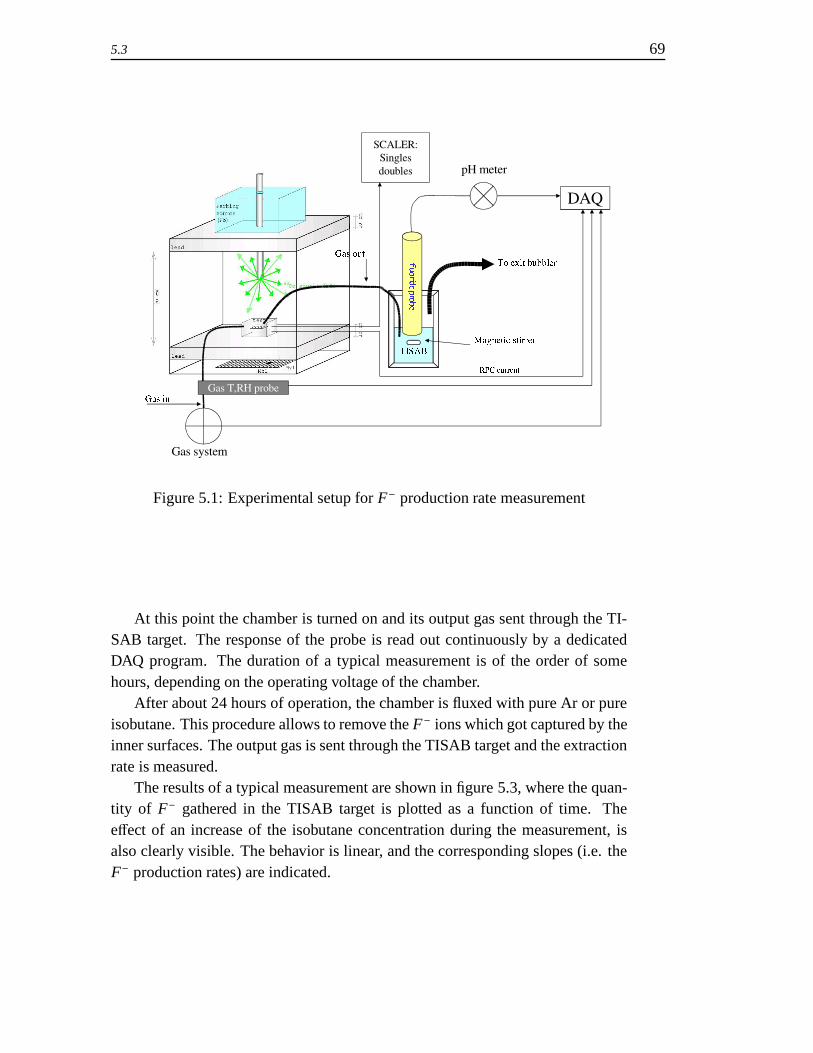
5.3 69
Figure 5.1: Experimental setup for F− production rate measurement
At this point the chamber is turned on and its output gas sent through the TI-SAB target. The response of the probe is read out continuously by a dedicatedDAQ program. The duration of a typical measurement is of the order of somehours, depending on the operating voltage of the chamber.
After about 24 hours of operation, the chamber is fluxed with pure Ar or pureisobutane. This procedure allows to remove the F− ions which got captured by theinner surfaces. The output gas is sent through the TISAB target and the extractionrate is measured.
The results of a typical measurement are shown in figure 5.3, where the quan-tity of F− gathered in the TISAB target is plotted as a function of time. Theeffect of an increase of the isobutane concentration during the measurement, isalso clearly visible. The behavior is linear, and the corresponding slopes (i.e. theF− production rates) are indicated.

70 Chapter 5. F− production in RPCs
-30
-10
10
30
50
70
90
110
130
150
-1.1 -0.6 -0.1 0.4 0.9 1.4 1.9 2.4
log([NaF])
pro
be
resp
ons
e (m
V)
Figure 5.2: F− probe calibration curve
5.3 Dependence of the F− production rate on theisobutane concentration
It has long been known that RPCs operated with fluoride compound gasesshow better performaces in terms of long time operation when the concentrationof isobutane in the gas mixture is increased. Being the production of F− one ofthe causes of ageing in RPCs, it should be expected that the presence of isobutanecan somehow influence the F− production and accumulation inside the chamber.
In order to test this hypothesis, the F− production rate has been measuredby operating the chamber with different gas mixtures. A chamber operating instreamer mode fluxed with a binary (TFE/isobutane) mixture has been used forthese measurements. The results are shown in figure 5.4.
The main consideration which can be done is that at constant total gas flow,the F− production rate decreases when the isobutane percentage is increased. Thedata clearly exclude that this decrease is due only to the decrease in concentrationof TFE, which in this mixture is the only F− source. Indeed, when decreasing theTFE concentration from 95% to 80% (i.e. increasing the isobutane from 5% to
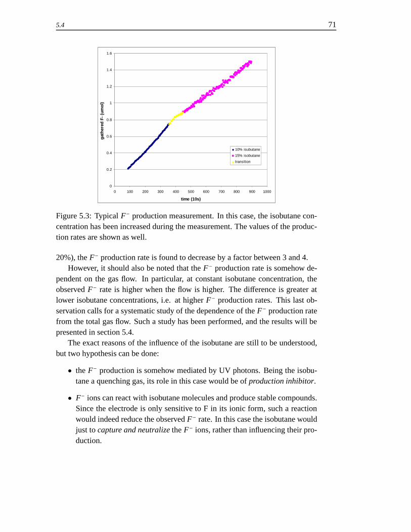
5.4 71
0
0.2
0.4
0.6
0.8
1
1.2
1.4
1.6
0 100 200 300 400 500 600 700 800 900 1000
time (10s)
gat
her
ed F
- (u
mo
l)
10% isubutane
15% isobutane
transition
Figure 5.3: Typical F− production measurement. In this case, the isobutane con-centration has been increased during the measurement. The values of the produc-tion rates are shown as well.
20%), the F− production rate is found to decrease by a factor between 3 and 4.However, it should also be noted that the F− production rate is somehow de-
pendent on the gas flow. In particular, at constant isobutane concentration, theobserved F− rate is higher when the flow is higher. The difference is greater atlower isobutane concentrations, i.e. at higher F− production rates. This last ob-servation calls for a systematic study of the dependence of the F− production ratefrom the total gas flow. Such a study has been performed, and the results will bepresented in section 5.4.
The exact reasons of the influence of the isobutane are still to be understood,but two hypothesis can be done:
• the F− production is somehow mediated by UV photons. Being the isobu-tane a quenching gas, its role in this case would be of production inhibitor.
• F− ions can react with isobutane molecules and produce stable compounds.Since the electrode is only sensitive to F in its ionic form, such a reactionwould indeed reduce the observed F− rate. In this case the isobutane wouldjust to capture and neutralize the F− ions, rather than influencing their pro-duction.

72 Chapter 5. F− production in RPCs
0.E+00
1.E-03
2.E-03
3.E-03
4.E-03
5.E-03
6.E-03
7.E-03
0 5 10 15 20 25
Isobutane (%)
F-
rate
(um
ol/1
0s)
30 cc/min
60 cc/min
Figure 5.4: F− production rate as a function of isobutane concentration for twodifferent total gas fluxes
5.4 The effect of the gas flow in F− production andaccumulation
As discussed in section 5.3, the F− production rate is found to be dependent onthe gas flow at which the chamber is operated. In order to investigate this effect, aspecific set of measurements was carried on.
The F− rate measured by the electrode is indeed due to the combination ofdifferent effects:
• the actual production of F− ions in the gas
• the partial accumulation of the ions on the internal surfaces of the plates
Some measurements of the accumulation process can be easily performed. Wedefine the attachment rate as the difference between the rate of the actual produc-tion inside the chamber and the rate which is measured by the electrode. What-ever the exact chemical reactions involved in the attachment are, some preliminaryconsiderations can be done:
• the attachment rate is likely to be inversely proportional to the gas flow
5.4 73
• it is reasonable to suppose that the attachment rate is proportional to theproduction rate itself.
In order to study the attachment rate, two identical chambers were seriallyconnected to the same gas line, with the downstream one turned off. The upstreamone was on the contrary operated at working point and the F− rate was measuredboth at the exit of the first chamber and at the exit of the second chamber. Thedifference between the two rates is a measurement of the attachment rate in thesecond chamber. Under the hypothesis that the two chambers behave in the sameway for what concerns the F− attachment, this measure allows to estimate whatthe attachment in the first chamber is, and thus to calculate the real productionrate.
The isobutane concentration in gas mixture and the operating current havebeen fixed at 10% and 10µA respectively, and the total gas flow has been set todifferent values, in the range 5÷60cc/min. Being φ1 the F− rate measured afterthe first chamber and φ2 the F− rate measured after the second chamber, the theabsorption factor is defined as
A =φ1 − φ2
φ1(5.9)
and represents the fraction of F− which is entrapped inside the second cham-ber. Figure 5.5 shows the absorption factors measured as a function of the totalgas flow. Remarkably the observed behavior is not inversely proportional to thegas flow, as clearly shown in figure 5.6, where the same data are plotted as afunction of the inverse of the gas flow. The reason of this behavior is still to beunderstood.
Once the absorption factor has been measured, it is possible to correct thevalue of φ1 in order to account for the fluorine ions attached into the first chamber.The corrected values, shown in figure 5.7 as a function of the total gas flow, aresubstantially in agreement with the hyposthesis of a constant F− production.
As already discussed in section 5.2.1, the chambers used for the tests pre-sented in this chapter were periodically fluxed with pure Ar, in order to removethe fluorine ions from the inner surface of the plates. Figure 5.8 show the F− con-centration in the target solution as a function of time for a chamber fluxed withpure Ar at 100cc/min. The current driven by the gap operated in Ar has beenswitched from 0 to 10µA, thus causing an increase of the extraction rate by a fac-tor 20. The dependence of the extraction rate in pure Ar on the operating current
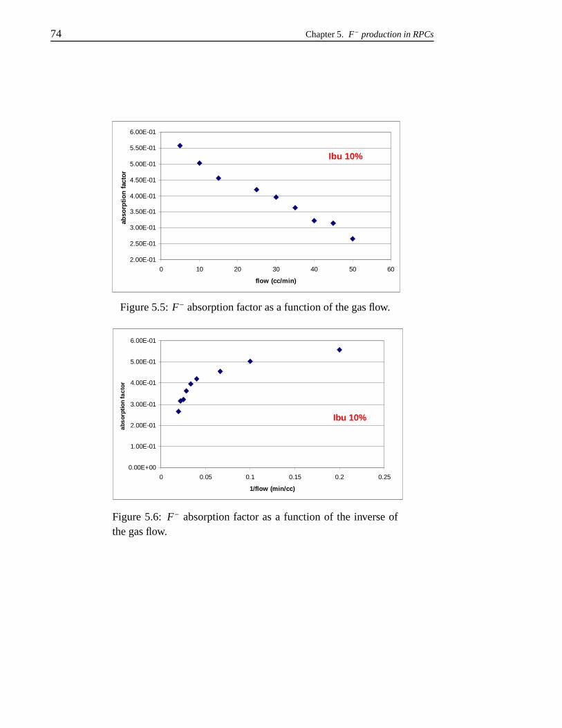
74 Chapter 5. F− production in RPCs
2.00E-01
2.50E-01
3.00E-01
3.50E-01
4.00E-01
4.50E-01
5.00E-01
5.50E-01
6.00E-01
0 10 20 30 40 50 60
flow (cc/min)
abso
rpti
on
fac
tor
Ibu 10%
Figure 5.5: F− absorption factor as a function of the gas flow.
0.00E+00
1.00E-01
2.00E-01
3.00E-01
4.00E-01
5.00E-01
6.00E-01
0 0.05 0.1 0.15 0.2 0.25
1/flow (min/cc)
abso
rptio
n fa
ctor
Ibu 10%
Figure 5.6: F− absorption factor as a function of the inverse ofthe gas flow.

5.5 75
0.00E+00
5.00E-04
1.00E-03
1.50E-03
2.00E-03
2.50E-03
3.00E-03
3.50E-03
4.00E-03
4.50E-03
5.00E-03
0 10 20 30 40 50 60
flow (cc/min)
corr
ecte
d p
rod
uct
ion
rat
e (u
mo
l/10
s)
Ibu 10%
Figure 5.7: F− production rate corrected using the measured absorption factor, asa function of the total gas flow.
has been found indeed to be linear (in the region above 2µA), as shown in figure5.9.
5.5 F− production as a function of the working cur-rent: avalanche and streamer working regimes
A clear knowledge of the exact dependence of the F− production on the work-ing current is of course needed for any long term use of RPCs, in which the op-erating voltage needs to be chosen in order to minimize any ageing effect due toF− pollution. Moreover, as discussed in section 3.4 RPCs can be operated, by aproper choice of the gas mixture and operating voltage, in two different regimes:avalanche and streamer. The study of the F− production for each regime is ofgreat interest, being for example the streamers characterized by the abundance ofUV photons, which is not true for avalanches. Therefore any difference in the pro-duction rate between avalanches and streamers can in principle give informationon the actual F− production mechanism.
A dedicated set of measurements has been performed in order to investigatethe abovementioned problems. The F− production rate has been measured forRPCs operated with binary and ternary mixtures, thus working in streamer andavalanche mode respectively. The exact composition of each mixture is shown in
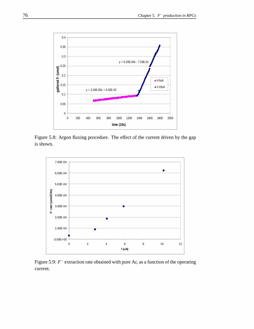
76 Chapter 5. F− production in RPCs
0
0.05
0.1
0.15
0.2
0.25
0.3
0.35
0.4
0 200 400 600 800 1000 1200 1400 1600 1800 2000
time (10s)
gath
ered
F- (
umol
)
I=0uA
I=10uAy = 3.24E-05x + 5.02E-02
y = 6.20E-04x - 7.53E-01
Figure 5.8: Argon fluxing procedure. The effect of the current driven by the gapis shown.
0.00E+00
1.00E-04
2.00E-04
3.00E-04
4.00E-04
5.00E-04
6.00E-04
7.00E-04
0 2 4 6 8 10 12
I (uA)
F-
rate
(u
mo
l/10s
)
Figure 5.9: F− extraction rate obtained with pure Ar, as a function of the operatingcurrent.

5.5 77
table 5.2. For each mixture, two different measurements of the F− production rateas a function of the working current were done:
mixture components composition
binary C2H2F4/i–C4H10 90/10tertiary C2H2F4/i–C4H10/S F6 89.5/10/0.5
Table 5.2: Gas mixtures used for avalanche vs streamer comparisons
• measurement at constant source irradiation, in which the current was in-creased by increasing the operating voltage of the chamber
• measurement at constant working point, in which the current variation isobtained increasing the irradiation rate (i.e. reducing the distance betweenthe source and the chamber). In this case the operating voltage was adjustedin order to compensate the voltage drop across the plates due to the currentdriven by the gap, thus maintaining a constant working point.
The results are shown in figure 5.10 and they clearly show the following ef-fects:
• at low working currents (<4µA) the chamber behaves always in the sameway, with no dependence on the gas mixture and the operating regime
• at higher working currents the binary mixture shows an effect of saturationof the F− production rate in spite of the increasing operating current
• the ternary mixture shows a behavior similar to the binary one when kept atconstant working point, while the plateau disappears if the operating voltageis increased under constant irradiation, in correspondence with the forma-tion of streamers in the gas. In these conditions, the F− production rateappears to rapidly increase when the operating voltage is increased.
In the ternary gas mixture there are indeed two sources of fluorine ions: C2H2F4
and S F6. The behavior of the chamber with ternary mixture operated at volt-ages above its optimal working point allows to conclude that at normal operatingvoltages the only significant contribution to the F− production rate is due to theC2H2F4. In fact in this region the binary and ternary mixtures produce the sameamount of fluorine ions. On the other hand, the presence of S F6 determines an
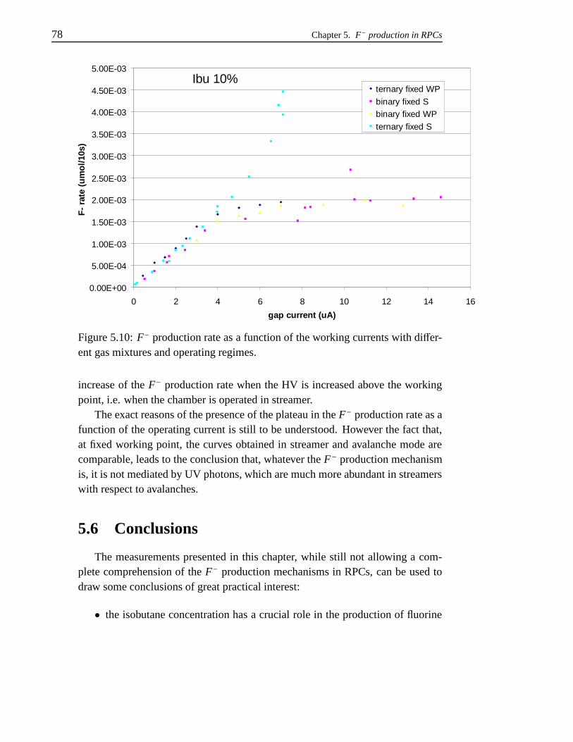
78 Chapter 5. F− production in RPCs
0.00E+00
5.00E-04
1.00E-03
1.50E-03
2.00E-03
2.50E-03
3.00E-03
3.50E-03
4.00E-03
4.50E-03
5.00E-03
0 2 4 6 8 10 12 14 16
gap current (uA)
F-
rate
(u
mo
l/10s
)ternary fixed WP
binary fixed Sbinary fixed WP
ternary fixed S
Ibu 10%
Figure 5.10: F− production rate as a function of the working currents with differ-ent gas mixtures and operating regimes.
increase of the F− production rate when the HV is increased above the workingpoint, i.e. when the chamber is operated in streamer.
The exact reasons of the presence of the plateau in the F− production rate as afunction of the operating current is still to be understood. However the fact that,at fixed working point, the curves obtained in streamer and avalanche mode arecomparable, leads to the conclusion that, whatever the F− production mechanismis, it is not mediated by UV photons, which are much more abundant in streamerswith respect to avalanches.
5.6 Conclusions
The measurements presented in this chapter, while still not allowing a com-plete comprehension of the F− production mechanisms in RPCs, can be used todraw some conclusions of great practical interest:
• the isobutane concentration has a crucial role in the production of fluorine

5.6 79
ions, and thus in the ageing of the detector. In particular, higher concentra-tions have proven to be very effective in reducing the observed F− produc-tion rate.
• the gas flow, on the other hand, has been shown to be an important parameterto reduce the deposit of F− ions on the inner surface of the gap.
• fluxing the chambers with pure Ar is an effective procedure for removingF− residuals from the inner surface of the plates. This effect is amplifiedwhen the current driven by the gas is different from zero.
• the S F6, which is fundamental to operate the RPCs in avalanche mode, is onthe other hand a major source of F− ions when operated in streamer mode,in spite of its low concentration.
Chapter 6
RPC simulation in the ATLASoffline framework using the Geant4toolkit
Simulation has a crucial role in high energy physics. It is indeed widely usedfor:
• the design of the experimental setup and the evaluation of its discovery po-tential;
• the development, test and optimization of the analysis and reconstructiontools;
• the measurement of physical quantities such as cross sections.
The simulation toolkit most widely used in the high energy physics communityhas been for a long time Geant3. It has been continuously developed for 15 years,but its last version (Geant3.2.1) has been released on March 1994 and is written inFORTRAN. It has been used not only in high energy physics simulations, but alsoin nuclear physics, and in the development of medical applications. One of thedisadvantages of Geant3 is the lack of a native implementation of the simulationof the hadronic processes, for which it relies on external packages.
6.1 The Geant4 Toolkit
Geant4 is a completely new toolkit, rather than a new release of Geant3. It isbased on an object oriented architecture, implemented using C++. It is in con-
80
6.2 81
tinuous development, and among its features there is a native implementation ofhadronic physics.
The Object Oriented approach ensures code maintainability along the numberof years foreseen for LHC experiment. Moreover, the implementation of physicalprocesses has been designed to be highly modular, thus allowing for the easy in-sertion of new processes.
The core components of the toolkit are known as the Geant4 kernel. The ker-nel is responsible for the simulation, i.e. it completely manages the run, takingcare of all the operations needed for the propagation in the simulated detector ofthe particles generated in each event. In order to carry out all its tasks, the kernelneeds to know from the user:
• a geometrical description of the volumes in which the particles will be prop-agated, together with an accurate description of the materials each volumeis made of;
• the list of the physical processes to be simulated for each kind of particle;
• a mechanism to generate the primary vertices of the events to be simulated.
A detailed description of the kernel internals is beyond the scope of this chap-ter, and can be found in [25] and in the Geant4 documentation, freely available onthe Geant4 official web site.
Hit production in Geant4 is provided by Sensitive Detectors. If a certain vol-ume described in the geometry is supposed to generate signals when crossed bysome kind of particle, it must be associated to a properly implemented Sensi-tive Detector, which is an instance of a class different from the one describingthe "real" geometry (tracking geometry in the following). The clear separationbetween Sensitive Detectors and Geometry classes allows to easily decouple thedescription of the tracking geometry from the one of the readout geometry. Eachtime a particle trajectory crosses a volume which can generate hits, the kernel isresponsible for calling the corresponding Sensitive Detector, which implementsthe hit generation algorithms. Hence, the Sensitive Detector generates a list ofhits, which are stored for further processing.
The RPCSensitiveDetector class has been implemented to provide the gen-eration mechanism for hits generated in the barrel trigger chambers.

82 Chapter 6. RPC simulation in the ATLAS offline framework using the Geant4 toolkit
6.2 ATHENA: the ATLAS offline framework
ATHENA [26] is a control framework based on the GAUDI architecture orig-inally developed by the LHCb experiment. This architecture has been extendedthrough collaboration with ATLAS, and an experiment neutral implementation,also called GAUDI, has been created. Athena is the result of this kernel frame-work, together with ATLAS-specific enhancements, such as the event data modeland event generator framework. The collaboration between LHCb and ATLAS isin the process of being extended to allow other experiments to also contribute newarchitectural concepts and concrete implementations to the kernel GAUDI frame-work.
It is intended that almost all software used in physics, whether for event gen-eration, reconstruction or analysis, will be in the form of specializations of a fewspecific components, where specialization means adding functionalities to a stan-dard component while keeping its interface the same. Within the applicationframework this is done by deriving new classes from one of the base classes:DataObject, Algorithm, Converter. Anything which has as its origin aconcept such as hit, point, vector, trajectory, i.e. a clear quantity-like entity shouldbe implemented by deriving a class from the DataObject base class. On the otherhand anything which is essentially a procedure , i.e. a set of rules for performingtransformations on more data-like objects, or for creating new data-like objectsshould be designed as a class derived from the Algorithm base class.
The role of an algorithm is to take input data, manipulate it and produce newoutput data. In general, an algorithm will be configurable: it will require certainparameters, such as cut-offs, upper limits on the number of iterations, convergencecriteria, etc., to be initialized before the algorithm may be executed. These param-eters may be specified at run time via job options files.
In ATHENA data objects produced by Algorithms are posted to a commonarea in memory from where other modules can access them and produce new dataobjects. The Transient Data Store (TDS) is the mechanism to provide such a com-mon area in the Gaudi architecture: an Algorithm creates a data object and post itinto the TDS, thus allowing other Algorithms to access it. Once an object is postedinto the store, the TDS takes ownership of it and manages its lifetime accordingto preset policies, removing, for example, a TrackCollection when a new event isread. StoreGate (SG) is the ATLAS implementation of the TDS. It manages thedata objects in transient form, as well as their transient/persistent conversion.

6.4 83
6.3 ATLAS Muon digitization
The Muon Digitization software packages have been completely re-written tooperate on Geant4 hits. It is independent of the Geant4 detector simulation, andruns within the ATHENA framework. The Muon Digitization consists of fouralgorithms, one for each muon technology (XXX_Digitization packages, whereXXX =MDT, RPC, TGC, CSC). It provides the production of collections of sim-ulated muon digits out of muon hit collections from the Geant4 simulation, whereboth the input and the output objects are assumed to be in SG. In the present archi-tecture, muon digits are converted to Raw Data Objects (RDOs) or to byte streamsbefore undergoing the persistent storage. RDOs are the output of the readout elec-tronic, thus are the constituents of the byte stream.
The goal of the muon digitization is to simulate the output signal of the muondetector in ATLAS given the output of the Geant4 detector simulation. The dig-itization process consists of two steps: in first, the output of the detector simula-tion, henceworth refereed to as Geant4 hits, is converted to muon digits. In thesecond step, the muon digits are converted to RDO from which the byte stream(the electronic output) is obtained. The muon digits are objects that can be feddirectly in the muon reconstruction, thus are known as Reconstruction Input Ob-jects (RIO). The muon off-line reconstruction dataflow starts from the raw data,the byte stream. The byte stream is read into the TDS as transient RDO dataobjects. In a subsequent steps, the RDO are converted into RIO (digits and orclusters), through calibration services, pedestal and noise handling, etc. The stepRDO→RIO is where the raw data is “prepared” before being fed into the off-linereconstruction. It thus follows that the muon digitization operates in the reversesteps of the off-line reconstruction dataflow, by producing the RIO first, then theRDO (or byte stream subsequently).
6.4 RPC digitization
6.4.1 From hits to digits
RPC hits are generated by the SensitiveDetector (SD) which assigns to thema Simulation Identifier (SimID), uniquely identifying the gas gap each hit is reg-istered in. The position of the hit in the reference system of the gas gap is alsostored, together with the time from the beginning of the event, i.e. the time offlight of the particle generating the hit. RPC hits are represented in the simulation

84 Chapter 6. RPC simulation in the ATLAS offline framework using the Geant4 toolkit
RPCHit RPCDigit
SimID of the gas gap OID of the stripPosition of the hit wrt the gas gap
Hit time (time of flight of the particle) Global time (tof + strip propagation)
Table 6.1: The information included in RPC hits and digits
code by instances of the class RPCHit.The digitization process takes care of adding to the hits the information nec-
essary for further analysis (for example trigger algorithm simulation and trackreconstruction). It translates any SimID to a Standard Offline Identifier (OID),which is used by the other ATHENA algorithms to uniquely identify RPC stripsin the muon spectrometer. Using the position information provided by the hits, thedigitization can properly calculate the propagation time of each electronic signalalong its strip, add it to the time of flight of the hit and assign this global timeto the digit. The information obtained is stored in a new instance of the classRPCDigit and posted in StoreGate for further processing. The main differencesbetween RPC hits and digits are summarized in table 6.1
6.4.2 Cluster simulation
When a particle generates an avalanche in an RPC, charge signals are induced(and detected) on the readout strips. A set of n adjacent strips with signals is calleda cluster of size n. In the RPC operation, due to possible signal induction on morethan one strip, cluster sizes are in general greater than 1, with an average clustersize at working point typically of 1.3. The hit production mechanism providedby the ATLAS Geant4 simulation does not include a tool for proper simulation ofclusters. Thus a particle generates hits on only one strip, except when secondaries(for example δ) are produced and detected by neighboring strips.
The impact point along a strip is known to influence the size of the clusterthe hit will generate. Figure 6.4.2 shows for example the probability to observea cluster of size 1 as a function of the impact point of the track along the strip.The strip pattern is also represented. The probability is normalized to the numberof clusters with sizes 1 or 2, i.e. for each bin, the complement to unity gives theprobability to have a cluster with size 2. From the plot it is clear that, for example,a muon crossing the region between two adjacent strips will most likely generatea cluster of size 2, whereas a track passing in the middle of one strip would induce

6.4 85
ClusterSize=1 (single hit)
ClusterSize=2
Figure 6.1: RPC clusters
Strips support
StripsImpact point (mm)
cs=1
pro
babi
lity
Figure 6.2: Probability to observe cluster size 1 as a function of the impact pointalong the strip.
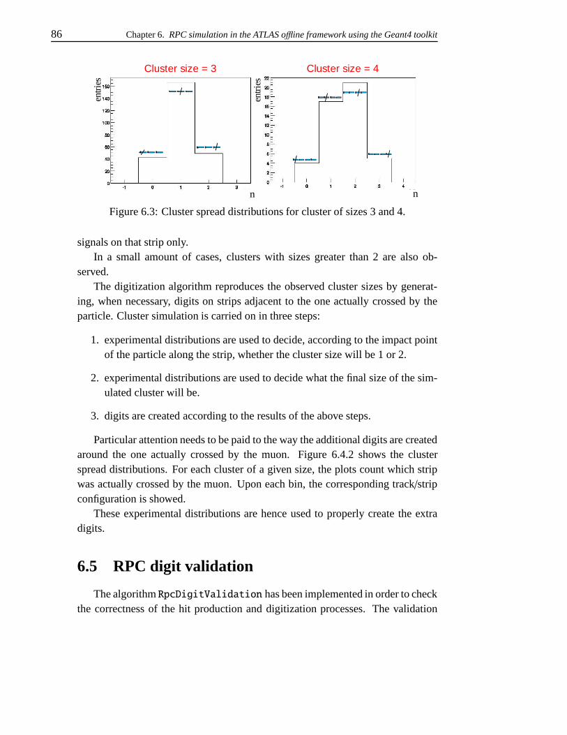
86 Chapter 6. RPC simulation in the ATLAS offline framework using the Geant4 toolkit
n n
entri
es
entri
es
Cluster size = 3 Cluster size = 4
Figure 6.3: Cluster spread distributions for cluster of sizes 3 and 4.
signals on that strip only.In a small amount of cases, clusters with sizes greater than 2 are also ob-
served.The digitization algorithm reproduces the observed cluster sizes by generat-
ing, when necessary, digits on strips adjacent to the one actually crossed by theparticle. Cluster simulation is carried on in three steps:
1. experimental distributions are used to decide, according to the impact pointof the particle along the strip, whether the cluster size will be 1 or 2.
2. experimental distributions are used to decide what the final size of the sim-ulated cluster will be.
3. digits are created according to the results of the above steps.
Particular attention needs to be paid to the way the additional digits are createdaround the one actually crossed by the muon. Figure 6.4.2 shows the clusterspread distributions. For each cluster of a given size, the plots count which stripwas actually crossed by the muon. Upon each bin, the corresponding track/stripconfiguration is showed.
These experimental distributions are hence used to properly create the extradigits.
6.5 RPC digit validation
The algorithm RpcDigitValidation has been implemented in order to checkthe correctness of the hit production and digitization processes. The validation
6.5 87
has been performed generating single muon events in the barrel, with no physicsprocesses activated but transportation. For each event, the algorithm executionproceeds as described in the following:
• for each muon, its direction at the generation vertex is retrieved from theMonteCarlo information. With no physics processes activated, this directionis a good approximation of the muon trajectory.
• for each RPC digit, its distance from the muon trajectory is calculated
• for each of the three RPC layers (Middle-lowPT, Middle-Pivot, Outer), theclosest digit to the muon is selected
• the fields of the OIDs of the selected digits are stored in an ntuple, togetherwith the direction of the muon.
The resulting ntuple can be used to validate both the RPCSensitiveDetectorand the RPCDigitization since it can easily spot any mistake in the generationof the SimID and in its translation to OID. For example the directions of the muonsnot producing any digit, or which produce digits too far from the track can be ana-lyzed. In figure 6.4 the η and ϕ directions of muons not producing any RPC digitsare plotted. These inefficiencies of the RPC system are concentrated, as expected,in regions not instrumented with RPCs:
• the feet of the ATLAS detector
• the ribs of the barrel magnet system
• the central (η = 0) crack
• the elevators
• the endcap regions (|η| > 1)
A similar plot has been produced for the outer stations and didn’t show anyabnormal inefficient region. With the same procedure, it is possible to look fordigits which are created in the wrong place.

88 Chapter 6. RPC simulation in the ATLAS offline framework using the Geant4 toolkit
RibsFeet
Central crackElevator
Figure 6.4: RPC digitization validation.

Chapter 7
The di-muon LVL1 trigger in theATLAS muon spectrometer
7.1 The ATLAS LVL1 trigger implementation
A general description of the Level 1 trigger and of the muon spectrometer hasbeen already given in chapters 1 and 2. As specialized trigger detectors, RPCs areused in the barrel part (|η| < 1.05) of the muon spectrometer, and TGCs, Thin Gapwire Chambers, in the end-cap.
RPCs are disposed in three stations, two of them (RPC1 and RPC2) cover theinternal and external faces of the middle precision chamber and the third (RPC3)is located close to the external precision chamber, as shown in figure 7.1. Eachstation is composed of an RPC doublet with read-out in two orthogonal views, ηand ϕ, referred as bending and non-bending projections respectively.
The barrel is divided in two half-barrels, symmetric with respect to η = 0, andazimuthally segmented in octants; each octant is further subdivided in two parts,referred as Large and Small sectors (see figure 7.2). RPC chambers are classi-fied, according to their location, into BML (Large sectors of RPC1 and RPC2),BMS (Small sectors of RPC1 and RPC2), BOL (Large sectors of RPC3) and BOS(Small sectors of RPC3).
The trigger logic is based on coincidences between different stations, one ofthe inner two stations being chosen as pivot. The two innermost stations are usedto trigger low-pT muons (mainly for b-physics studies), while the outermost isused to trigger high-pT muons.
The trigger logic is implemented through Coincidence Matrices (CM), to which
89

90 Chapter 6. The di-muon LVL1 trigger in the ATLAS muon spectrometer
Figure 7.1: View of a standard barrel sector. The RPCs are represented by shadedboxes.

7.1 91
BarrelSector
Large
Barrel Sector
Small
Figure 7.2: Azimuthal view of one half-barrel octant. Small units are placed incorrespondence of magnet coils.
the RPC strips are connected. Four CMs, two in η and two in ϕ, form a Pad. Theintersection of one η-CM and one ϕ-CM within a Pad gives a ROI (Region OfInterest) of size ∆η × ∆ϕ ' 0.1 × 0.1. The trigger response is given evaluatingthe so called Coincidence Windows, as schematically shown in figure 7.3. In thebarrel, where a muon is seen to leave a hit in both of the low-pT stations, the pro-jective extrapolation of the hit in station 2 to station 1 can be made assuming themuon path to be a straight line (i.e. the infinite momentum approximation) withthe origin at the interaction point. The distance between the extrapolated pointin station 1 and the actual hit detected is defined as the separation parameter, d.In the end-cap system the low-pT trigger coincidence is made using station 3 andstation 2.
The coincidence windows of the level-1 muon-trigger are designed to offermomentum discrimination by including muons above threshold and excludingthose below threshold which will be bent outside the coincidence window. The pT
resolution at fixed threshold in turn is a function of the trigger detector geometry(in particular the lever arm between stations 1 and 2, and station 3), the mag-netic field strength and its inhomogeneities, the Coulomb scattering in the centralcalorimeter and the width of the interaction region.
The sizes of the trigger windows that determine the pT threshold have been

92 Chapter 6. The di-muon LVL1 trigger in the ATLAS muon spectrometer
Figure 7.3: Schematic view of the coincidence-window-based muon LVL1 trigger.
computed [27] for the proposed trigger system by tracking single muons throughthe ATLAS detector using Monte Carlo simulation techniques. The size of a coin-cidence window is defined such that 90% of the muons of each charge within thedetector acceptance, generated with transverse momentum equal to the threshold,are accepted.
The coincidence window is not symmetric around the extrapolated point ofthe infinite momentum path: muons of a given charge, bending towards high |z|regions (in the barrel) or high r regions (end-cap), cross station 1 at a distancefrom the extrapolated point larger than that for muons of opposite charge. Thiseffect increases with |η| in the barrel and with r in the end-cap. This leads to asym-metric coincidence windows, formed by independent left and right half-windows.The difference between the right and left halfwindow is 7/10 cm in the large/smallchambers at |η| 0.9 in the barrel and 3.5 cm at |η| close to 1 in the end-cap. Thesize of each half-window is evaluated accounting for the relative trigger efficiencyof positive and negative muons independently, to minimize possible effects oncharge-asymmetry measurements. Figure 7.4 shows the working principle of thecoincidence-windows-based ATLAS LVL1 muon trigger.
The CM board produces an output pattern containing the low-pT trigger re-
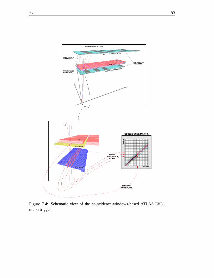
7.1 93
+
PIVOT PLANE
HIGH PT COINCIDENCE PLANE
LOW PT COINCIDENCE PLANE
Z
Y
RPC strips
RPC strips
COINCIDENCE
PIVOT PLANE
COINCIDENCEWINDOW HPT
COINCIDENCEWINDOW LPT
+
X
CM INPUT
PLANE
CM INPUT
Infinite Momentum Track
COINCIDENCE MATRIX
RPC TRIGGERCHAMBERS
COINCID
ENCE ROAD
RoI
Figure 7.4: Schematic view of the coincidence-windows-based ATLAS LVL1muon trigger

94 Chapter 6. The di-muon LVL1 trigger in the ATLAS muon spectrometer
sults for each pair of RPC doublets in the η or ϕ projection. The information oftwo adjacent CM boards in the η projection, and the corresponding information ofthe two CM boards in the ϕ projection, are combined together in the low-pT PadLogic (Pad) board. The four low-pT CM boards and the corresponding Pad boardare mounted on top of the second RPC station. The high-pT trigger logic receivesas an input the hits on the third station and the output pattern of the low-pT triggeralgorithm. The low-pT Pad board generates the low-pT trigger result and the asso-ciated RoI information. This information is transferred, synchronously at 40MHz,to the corresponding high-pT Pad board, mounted on the third RPC station, thatcollects the overall result for low- and high-pT .
The high-pT Pad board combines the low- and high-pT trigger results. Thecombined information is sent, synchronously at 40MHz, via optical links, to aSector Logic (SL) board, located in the counting room. Each SL board receivesinputs from seven (six) low-pT (high-pT ) Pad boards, combining and encodingthe trigger results of one of the 64 logic sectors into which the barrel trigger sys-tem is subdivided. The trigger data elaborated by the Sector Logic is sent, againsynchronously at 40MHz, to the Muon Interface to the Central Trigger Processor(µCTPI), located in the same counting room.
Data are read out from both the low- and high-pT Pad boards. These datainclude the RPC strip pattern and some additional information used in the LVL2trigger. The read-out data for events accepted by the LVL1 trigger are sent asyn-chronously to Read-Out Drivers (RODs) located in the counting room and fromhere to the Read-Out Buffers (ROBs). The data links for the read-out data areindependent of the ones used to transfer partial trigger results to the SL boards.
Figure 7.5 illustrates the segmentation of the LVL1 trigger system in the AT-LAS barrel. In each half barrel, one physical sector is divided in two logic sectors(i.e. it is readout by two SL boards). Approximate RoI, Pad and CM dimensionsare shown, as an example, for a small sector.
7.2 Rare beauty decay studies in the ATLAS detec-tor.
In certain rare B decays, the decay products provide a distinctive signaturethat can be used in the LVL1 trigger. These so-called self-triggering modes in-clude decays of the type Bd,s → µµ(X), which involve flavor-changing neutralcurrents (FCNC) and are strongly suppressed in the Standard Model, with pre-

7.2 95
Figure 7.5: Segmentation of the LVL1 barrel trigger.
dicted branching ratios typically in the range 10−5÷10−10. The high rate of B-hadron production foreseen in ATLAS will allow a very effective study of thesechannels.
For the purely muonic decays, ATLAS will be sensitive to branching ratios ofthe order of 10−9 and should be able to measure the branching ratio for Bs → µµ
assuming the Standard Model prediction. Large-statistics samples will be col-lected for decays of the type b→ (s, d)ll that give final states such as B0
d → K∗0µµ,B0
d → ρ0µµ and B0s → φ0µµ. This will allow precise measurements to be made
of the decay dynamics, as well as of the branching ratios, giving significant con-straints on new physics.
These rare decay modes are forbidden at the tree level in the Standard Model,i.e. the decays involve loop diagrams, thus being highly suppressed. In non-standard models of electroweak interactions, FCNC processes can be allowed atthe tree level and therefore the branching ratios of these rare decays would behigher. In addition, in the presence of new physics, additional particles may bepresent in the loops, thus increasing the decay probability.
In the context of Standard Model, the measurement of the branching frac-tions of the B → µµ(X) channels is of primary interest. The measurement of thebranching fractions of the decays B0
d → K∗0µµ and B0d → ρ0µµ allows the CKM
matrix-element ratio |Vtd |/|Vts| to be determined. The square of this ratio is useful

96 Chapter 6. The di-muon LVL1 trigger in the ATLAS muon spectrometer
Channel Signal BackgroundB0
d → µµ 4 93B0
s → µµ 27 93
Table 7.1: Number of expectedevents after three years at low lu-minosity (30 f b−1)
Channel Signal BackgroundB0
d → µµ 14 660B0
s → µµ 92 660
Table 7.2: Number of expectedevents after one year at low lu-minosity (100 f b−1)
also for the estimation of the ratio of the mass differences ∆ms/∆md in the B0d− B0
d
and B0s − B0
s systems, complementary to direct measurements of the oscillationperiods.
7.2.1 The channel Bd,s → µµ
As an example of the difficulties involved in the study of such rare decays, inthe following some results obtained from simulated events ([3]) will be summa-rized.
Simulations were made with the PYTHIA event generator. The Inner-Detectorresponse was fully simulated and the particles were reconstructed in the Inner De-tector. The muon reconstruction efficiency was assumed to be 85% for the LVL1trigger muon, and 95% for the other trigger levels. About 1500 signal events weresimulated in each channel, with pT (µ) > 6GeV and |η(µ)| < 2.5 for each muon.About 9000 background events were simulated and reconstructed.
The cuts applied for signal selection are:
• Decay length of B0> 0.7 mm
• Angle between pT of B0 and the line joining the primary and secondaryvertices < 1
• Isolated muons (no charged particles in a cone of 20)
Tables 7.1 and 7.2 ([3]) show the number of events (for both background andsignal) passing the cuts.
From the results reported above, it is clear that it is crucial, in order to increasethe significance of the signal for such channels, to increase the signal-to-noise ra-tio. The muons coming from B-physics di-muon sources are characterized bylow (< 6 GeV)pT values. Figure 7.6, for example, shows the pT distribution for

7.3 97
Tp4 5 6 7 8 9 10
entr
ies
500
1000
1500
2000
2500
3000
transverse momentum
Figure 7.6: pT distribution for muons coming from pp→ bb→ µµX processes.
muons coming from pp → bb → µµX processes. An enhancement of the signalcould therefore be obtained reducing the LVL1 muon trigger pT threshold. Un-fortunately, this would also increase the background contamination in the selectedsample. One of the possible improvements for the analysis of this kind of decaysis the implementation of a di-muon trigger.
7.3 The di-muon trigger
A trigger scheme with the possibility to discriminate events with two muonshas been foreseen in the ATLAS experiment, in order to increase the sensitivity ofthe detector to inclusive di-muon decays, which are the signature of many inter-esting processes, such as rare B decays. In the following, the results from a studyof the di-muon trigger performace in the barrel region are presented.
7.3.1 Geometrical overlaps
In order to increase the trigger acceptance of the muon spectrometer, severalregions of overlap between the trigger chambers are foreseen in the detector lay-out. A muon crossing one of these regions, may generate two different triggers,thus producing a false di-muon trigger. The trigger system must therefore beaware of the geometrical overlaps, in order to reject such fake double triggers.
Three kinds of geometrical overlaps are present in the barrel trigger chambers

98 Chapter 6. The di-muon LVL1 trigger in the ATLAS muon spectrometer
layout:
• ϕ overlaps between two adjacent sectors.
• η overlaps between two CMs belonging to the same pad.
• η overlaps between two CMs belonging to adjacent pads in the same sector.
An example of the first kind of overlaps is shown in 7.7, while the layout char-acteristics causing the second and third overlap typologies are shown in figures7.8 and 7.9 respectively.
In order to properly discriminate the fake double triggers, the trigger resultsfrom the CM operation can be flagged when the trigger originates from a stripin the pivot plane which is known to be in a region of geometrical overlap. Thehigher levels of the LVL1 trigger logic (i.e. Pad, SL and µCTPI) will afterwardstake care of identify and remove from the trigger results the fake double triggers.
In more detail, the removal of the fake double triggers by different parts of theLVL1 trigger logic proceeds as follows:
• the η overlaps between two CMs belonging to the same pad are solved by thepad itself, which indeed passes to the SL only one of the triggers detectedby its matrices, i.e. the one with the highest threshold.
• the η overlaps between two CMs belonging to adjacent pads in the samelogic sector are solved by the SL board the pads belong to. The SL collectsthe triggers from all its pads, and when it finds two triggers in two adjacentpads, both with the eta overlap flag asserted, it ignores one of them.
• finally, ϕ overlaps between two adjacent sectors can’t be solved by the bar-rel trigger logic, and the µCTPI is designed to deal with such overlaps. Itchecks the ϕ overlap flags of the triggers coming from the SL boards andproperly removes the fake double triggers. At this stage the overlaps be-tween the barrel and the endcap trigger systems (which will not be analyzedin this work) will also be solved.
7.3.2 Determination of the overlap flags
As discussed above, the trigger system needs to be aware of the strips whichare located in geometrically overlapping regions, and hence are likely to producefake double triggers. This information is stored in each CM configuration file.
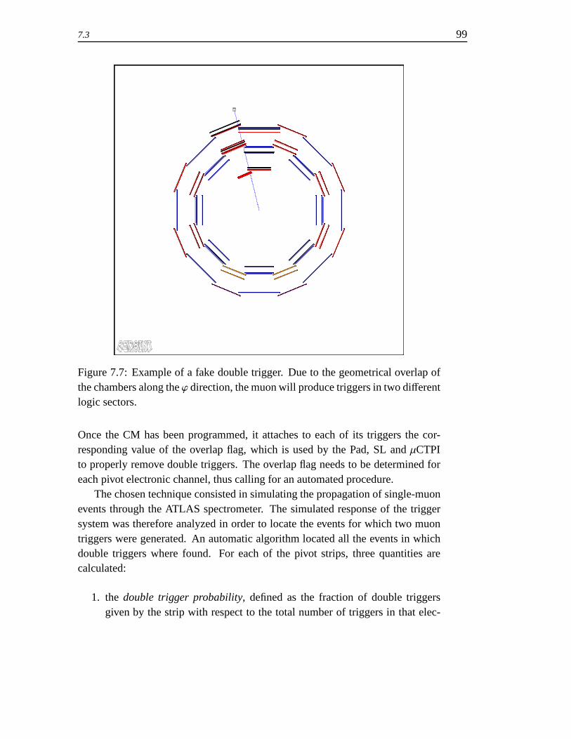
7.3 99
Figure 7.7: Example of a fake double trigger. Due to the geometrical overlap ofthe chambers along the ϕ direction, the muon will produce triggers in two differentlogic sectors.
Once the CM has been programmed, it attaches to each of its triggers the cor-responding value of the overlap flag, which is used by the Pad, SL and µCTPIto properly remove double triggers. The overlap flag needs to be determined foreach pivot electronic channel, thus calling for an automated procedure.
The chosen technique consisted in simulating the propagation of single-muonevents through the ATLAS spectrometer. The simulated response of the triggersystem was therefore analyzed in order to locate the events for which two muontriggers were generated. An automatic algorithm located all the events in whichdouble triggers where found. For each of the pivot strips, three quantities arecalculated:
1. the double trigger probability, defined as the fraction of double triggersgiven by the strip with respect to the total number of triggers in that elec-

100 Chapter 6. The di-muon LVL1 trigger in the ATLAS muon spectrometer
RPC
RPC
Figure 7.8: Eta overlap between two CMs in the same pad.
MDT
RPCRPC
RPC
Figure 7.9: Eta overlap between two adjacent pads. A muon track such the onereported here would generate triggers on two different pads in the same sector.
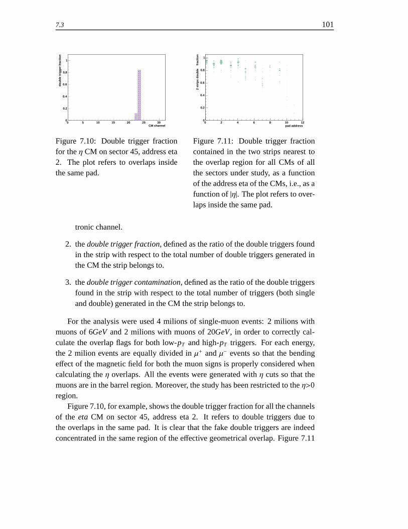
7.3 101
CM channel0 5 10 15 20 25 30
do
ub
le t
rig
ger
fra
ctio
n
0
0.2
0.4
0.6
0.8
1
Figure 7.10: Double trigger fractionfor the η CM on sector 45, address eta2. The plot refers to overlaps insidethe same pad.
pad address0 2 4 6 8 10 12
fra
ctio
n
2 st
rip
s d
ou
ble
0
0.2
0.4
0.6
0.8
1
Figure 7.11: Double trigger fractioncontained in the two strips nearest tothe overlap region for all CMs of allthe sectors under study, as a functionof the address eta of the CMs, i.e., as afunction of |η|. The plot refers to over-laps inside the same pad.
tronic channel.
2. the double trigger fraction, defined as the ratio of the double triggers foundin the strip with respect to the total number of double triggers generated inthe CM the strip belongs to.
3. the double trigger contamination, defined as the ratio of the double triggersfound in the strip with respect to the total number of triggers (both singleand double) generated in the CM the strip belongs to.
For the analysis were used 4 milions of single-muon events: 2 milions withmuons of 6GeV and 2 milions with muons of 20GeV , in order to correctly cal-culate the overlap flags for both low-pT and high-pT triggers. For each energy,the 2 milion events are equally divided in µ+ and µ− events so that the bendingeffect of the magnetic field for both the muon signs is properly considered whencalculating the η overlaps. All the events were generated with η cuts so that themuons are in the barrel region. Moreover, the study has been restricted to the η>0region.
Figure 7.10, for example, shows the double trigger fraction for all the channelsof the eta CM on sector 45, address eta 2. It refers to double triggers due tothe overlaps in the same pad. It is clear that the fake double triggers are indeedconcentrated in the same region of the effective geometrical overlap. Figure 7.11

102 Chapter 6. The di-muon LVL1 trigger in the ATLAS muon spectrometer
Figure 7.12: Fake double trigger frac-tion contained in the three strips near-est to the overlap region for all CMs ofall the sectors under study. Only CMswith more than 100 entries are consid-ered in this plot.
Figure 7.13: Fake double trigger frac-tion that is contained in the fourth stripnear the three considered in 7.12
reports the sum of the double trigger fraction registered by the two strips of eachCM which are the nearest to the actual overlap region, as a function of the η
address of the pads the double triggers are found in. The η address increases with|η|, so this plot shows that in the forward regions of the barrel the double triggerstend to interest more than two strips, as expected.
The results obtained for the ϕ overlaps are shown in figures 7.12 and 7.13. Asfor the η overlaps, these plots show the fraction of fake double triggers registeredin the strips adjacent to the actual geometrical overlap. In particular, figure 7.12shows that in the majority of the CMs, a fraction of fake double triggers greaterthan 80% is registered in just three strips, while figure 7.13 shows that typicallyadding a fourth strip to the three considered in figure 7.12 does not produce a greatincrease in the fraction of fake double trigger.
The ϕ fake double triggers were found to be 3.4% of the total ϕ triggers; thisratio decreases to 1.5% when calculated for the η projection.
Studying the results obtained from the fake double trigger analysis presentedabove, the following rules for the assignment of the overlap flags to the readoutchannels has been followed:
• as already discussed, the η overlaps between two CMs belonging to thesame pad does not require any flag to be set;
• for the η overlaps between adjacent pads, 7 strips are flagged in the regions

7.3 103
of the spectrometer illustrated in figure 7.9;
• for the ϕ overlaps, 3 strips are flagged; if they don’t account for at least80% of the fake double triggers in their CM, a fourth strip is added only ifit brings the fraction of fake double triggers above 80%
7.3.3 Performance study
Two tests have been performed to evaluate the impact of the overlap flagsdetermined as described above on the performances of the LVL1 muon trigger:
• a single muon sample is used to check the proper removal of the fake doubletriggers
• a di-muon sample is used to check the amount of real double triggers thatare lost due to the overlap removing mechanism.
In addition to the algorithm used to determine the overlap flags, which ana-lyzes the LVL1 trigger results looking for fake double triggers, a dedicated algo-rithm simulating the overlap solving functions of the µCTPI, has been developed.
These algorithms, applied on the LVL1 simulation results obtained for singlemuon events, showed that 22% of the fake double triggers was still not removedby the overlap solving routine. This is exactly what can be expected, consideringthe fact that the overlap flags were chosen in order to eliminate ∼80% of the fakedouble triggers.
The data sample used for the di-muon test are pp− > J/ψ(µµ)X events withthresholds on the pT of the two muons for the J/φ decay set to 6 and 3 GeV .The MonteCarlo information has been used to select the events according to thefollowing criteria:
• the event must present in the final state two muons with pT>6GeV (muonswith lowest pT would not be triggered anyway)
• both the muons must be in the barrel acceptance range (|η| < 1)
• the muons must be close to each other in space (∆ϕ < 0.1 and ∆η < 0.1). Adouble trigger indeed can be lost only in the case both the muons go throughthe same overlap region.

104 Chapter 6. The di-muon LVL1 trigger in the ATLAS muon spectrometer
1thr-2 0 2 4 6 8
2th
r
-2
0
2
4
6
8
Figure 7.14: Trigger thresholds of di-muon events passing the selection criteria.The ellipses show the cases in which one of the two triggers is considered "fake"by the overlap solving algorithm. The values of 1, 2, 3, 4, 5, 6 reported on theaxes correspond to the pT values of 6, 8, 10, 11, 20 and 40GeV respectively.
In addition to these cuts, in order to consider only clean events, the presenceof only two triggers (both with threshold different from 0) is required. The thresh-olds of the triggers are plotted, one vs the other, in figure 7.15. The value -1 isassigned by the overlap solving routine to the threshold of those triggers it has re-moved because of the overlap flags: such triggers are indicated by two ellipses inthe figure. The fraction of real double triggers which are lost due to the presenceof the overlap flags is therefore 0.58% of the total events, and it raises to 2.2% ifwe consider only the events in which both the muons gave triggers with non zerothreshold.
A similar analysis has been also performed on B → µµ events, the only dif-ference being that no constraint on the angular separation between the two muonshas been put, thus allowing to evaluate the global amount of events that are notproperly triggered. The results are shown in figure 7.14. One of the two muons iswrongly considered fake only in the 0.4% of the events giving two triggers.

7.4 105
1thr-1 0 1 2 3 4 5 6 7 8
2th
r
-1
0
1
2
3
4
5
6
7
8
Figure 7.15: Trigger thresholds of B → µµ events passing the selection criteria.The ellipses show the cases in which one of the two triggers is considered "fake"by the overlap solving algorithm. The values of 1, 2, 3, 4, 5, 6 reported on theaxes correspond to the pT values of 6, 8, 10, 11, 20 and 40GeV respectively.
7.4 Conclusions
The overlap solving mechanism of the ATLAS LVL1 muon trigger has beenfor the first time intensively tested with the final detector layout.
The overlap flags, needed by the trigger logic to properly handle fake doubletriggers due to geometrical overlap of the trigger detectors, have been determinedon a strip-by-strip basis by an automated procedure. In the case of ϕ overlapsbetween adjacent sectors, it has been shown that about 80% of the fake doubletriggers occur in the three strips nearest to the overlap region.
A pp− > J/ψ(µµ)X sample has been used to evaluate the fraction of realdouble triggers which is lost due to the overlap solving logic. This fraction hasbeen measured to be 0.58% of the selected events, raising to 2.2% if only eventswith both the triggers above threshold are considered.
A study performed on a B → µµ sample showed that one of the two muons iswrongly considered fake only in the 0.4% of the events giving two triggers.

Bibliography
[1] "The Large Hadron Collider - Conceptual Design", CERN/AC/95-05
[2] ATLAS Muon Collaboration; “ATLAS Muon Spectrometer Technical De-sign Report”, CERN/LHCC 97-22.
[3] ATLAS Collaboration; “Detector and Physics Performance Technical De-sign Report”, CERN/LHCC 99-14/15.
[4] W. Blum; ATLAS internal note MUON-NO-24 (1993).
[5] Detector Physics Group, ATLAS internal note MUON-NO-98 (1995).
[6] K. Nagai; “Thin Gap Chambers in ATLAS”, Nucl. Instrum. Methods A384(1996) 219.
[7] ATLAS Collaboration; “ATLAS First-Level Trigger Technical Design Re-port”, CERN/LHCC 97-22 (1998).
[8] R. Santonico and R. Cardarelli; “Development of Resistive plate coun-ters”,NIM, Nuclear Instruments and Methods in physiscs research 187(1981).
[9] P. Camarri et al.; “Streamer suppression with S F6 in RPCs operated inavalanche mode”, NIM, Nuclear Instruments and Methods in physiscs re-search A414 (1998).
[10] R. Cardarelli et al.; “Avalanche and streamer mode operation of resistiveplate chambers”, NIM, Nuclear Instruments and Methods in physics researchA382 (1996).
[11] R. Cardarelli, A. Di Ciaccio, R. Santonico; “Performance of a resistive platechamber operating with pure CF3Br,NIM, Nuclear Instruments and Methodsin physiscs research 333 (1993).
106

Bibliography 107
[12] M. Abbrescia et al.; “Resistive plate chambers working at high rate”, NIM,Nuclear Instruments and Methods in physiscs research B44 (1995).
[13] C. Bacci et al.; “Test of a resistive plate chamber operating with low gas am-plification at high intensity beams”, NIM, Nuclear Instruments and Methodsin physiscs research A352 (1995).
[14] R. Santonico; “Topics in resistive plate chambers ”, ‘Third InternationalWorkshop on Resistive Plate Chambers and related detectors’ on SCIEN-TIFICA ACTA Quaderni del dottorato (Universita’ degli studi di Pavia volIX (15 maggio 1996).
[15] A. Ferrari and P. Sala; ATLAS Internal Note MUON-NO-162 (1997).
[16] M. Angelone et al.; “Test of a resistive plate chamber under irradiation ofphotons and neutrons”, NIM, Nuclear Instruments and Methods in physicsresearch A355 (1995).
[17] S. Altieri et al.; “Gamma sensitivity simulation of Resistive Plate Cham-bers”, Fourth International Workshop on Resistive Plate Chamber and re-lated detectors 1999 (Bari).
[18] S. Agosteo et al.; “A facility for the test of large area muon chambers at highrate”, CERN-EP-2000-031, February 16th, 2000.
[19] E. Gennari et al.; “32 channel TDC VME board - User’s Manual”,http://sunset.roma2.infn.it/tdc/tdcboard.ps.
[20] G. Aielli et al.; "Electrical conduction properties of phenolic-melaminic lam-inates", Seventh International Workshop on Resistive Plate Chamber andrelated detectors 2003 (Clermont-Ferrand).
[21] G. Aielli et al.; "RPC ageing studies"; Proceedings of VCI 2001, NIM, Nu-clear Instruments and Methods in physiscs research A478 (2002) 271-276.
[22] G. Aielli et al.; "Further advances in aging studies for RPCs"; NIM, NuclearInstruments and Methods in physiscs research A518 (2003) 335-341.
[23] G. Aielli; Ph.D. thesis, University of Rome Tor Vergata, February 2001.

108 Bibliography
[24] G. Aielli et al.; “Performance of a large size RPC, equipped with the final AT-LAS front-end electronics, at X5-GIF facility”, NIM, Nuclear Instrumentsand Methods in physiscs research A456 (2000) 77.
[25] S. Agostinelli, J. Allison, K. Amako, J. Apostolakis, H. Araujo, P. Arce,M. Asai, D. Axen, S. Banerjee, G. Barrand et al.; "Geant4 - A SimulationToolkit", Nuclear Instruments and Methods A 506 (2003) 250-303
[26] "ATHENA Developer Guide", http://atlas.web.cern.ch/Atlas/GROUPS/SOFTWARE/OO/architecture/General/Documentation/ AthenaDeveloperGuide-8.0.0-draft.pdf
[27] F. Conventi; "The Simulation of the Level-1 muon trigger at LHC", PhDThesis
[28] M. Virchaux, D. Pomarède; "Persint Manual",http://atlasinfo.cern.ch/Atlas/GROUPS/MUON/ persint/Persint_manual.pdf

Aknowledgements
I would like to express my gratitude to Rinaldo Santonico, for his constantpresence during these years of work, and for having introduced me to the researchon Resistive Plate Chambers. I am also grateful to Anna Di Ciaccio, who followedme during my activities in the ATLAS software group, and patiently corrected thefirst drafts of this manuscript. For some of the results reported in this thesis I haveto thank Roberto Cardarelli’s intuitions and help.
Special thanks are due to Giulio Aielli, Barbara Liberti and Paolo Camarri, fortheir precious collaboration and friedship in the last three years.
I am also thankful to Luigi Di Stante, Enrico Pastori, Emiliano Paoletti, LuigiPasquali and to all the technical staff of the INFN-Roma2 ATLAS laboratories forreminding me, with their precious work, of how many things I am just not able todo.
The work on the Geant4 simulation of the ATLAS RPCs has been made eas-ier and pleasant by the collaboration with Adele Rimoldi and Daniela Rebuzzi, towhom I owe my gratitude.
For my work on the ATLAS LVL1 di-muon trigger, I profited from the experi-ence, suggestions and practical help of Leandro Nisati and Alessandro Di Mattia.
Finally my gratefulness goes to my family and my friends, for their love,friendship and patient support.
109