Via Cosimo Ridolfi, 10 – 56124 PISA – Tel. Segr. Amm. 050 2216231 Segr. Stud. 050 2216317 Fax 050 2216375

Cod. Fisc. 80003670504 - P. IVA 00286820501 - Web http://statmat.ec.unipi.it/ - E-mail: dipstat@ec.unipi.it

Università degli Studi di Pisa Dipartimento di Statistica e Matematica

Applicata all’Economia

Report n. 316

Endogenous restricted participation in general financial equilibrium:

existence results

Laura Carosi Michele Gori

Antonio Villanacci Pisa, maggio 2009 - Stampato in Proprio –

Endogenous restricted participation

in general financial equilibrium: existence results

Laura Carosi∗, Michele Gori†and Antonio Villanacci‡

May 8, 2009

Abstract

We consider an incomplete market model with numeraire assets. Each household facesan individual constraint on its participation in the asset market. In related literature, theconstraint is described by a function whose sole argument is the asset portfolio. On the contrary,in our analysis the constraint depends not only on the asset portfolio, but also on asset andgood prices - hence the reference to endogenous (in contrast to exogenous) in the title. We alsoanalyze the case in which some household is excluded from the trade of some asset. Existenceresults are provided using a homotopy argument.

JEL classification: D50; D52.Keywords: General equilibrium; Restricted participation; Financial markets; Existence of equi-

libria.

1 Introduction

This paper provides existence results for a pure exchange general equilibrium model with incompletemarkets and endogenous restricted participation. We consider the same model presented in Carosi,Gori and Villanacci (2009)1. Each household has only partial access, in a personalized manner tothe available set of assets. In related literature, the constraint is described by a function whose soleargument is the asset portfolio. On the contrary, in our analysis the constraint depends not onlyon the asset portfolio, but also on asset and good prices - hence the reference to endogenous (incontrast to exogenous) in the title. Each economies is described by endowments of commodities,utility functions, asset yield matrices, and restriction functions.

Assumptions on restriction functions are a natural generalizations to the endogenous setting ofthose used in Cass, Siconolfi and Villanacci (2001) in the exogenous case. It turns out that, in bothmentioned frameworks, those assumptions imply that the admissible portfolio set has nonemptyinterior - see Lemma 5 below. Therefore, they do not allow to cover the case in which somehousehold is excluded from the trade of some asset. Our proposed technique of proof can easilyaccomodate that economically meaningful situation.

The paper is organized as follows. In Section 2, we present the setup of the model. In Section 3,we show existence of equilibria in the case of restriction functions satisfying the proposed, standardset of assumptions; an homotopy argument is used. Finally, in Section 4, we show existence in thecase of some household asset demand for some asset being forced to be zero.

2 The model

Our model is the by now very standard two-period, pure exchange economy with uncertainty andboth commodities and assets. Spot commodity markets open in the first and second periods, and∗Dipartimento di Statistica e Matematica Applicata all’Economia, Universita di Pisa, E-mail: lcarosi@ec.unipi.it†Dipartimento di Matematica per le Decisioni, Universita degli Studi di Firenze, E-mail: michele.gori@unifi.it.‡Dipartimento di Matematica per le Decisioni, Universita degli Studi di Firenze, E-mail: anto-

nio.villanacci@unifi.it.Our research has been partially supported by M.I.U.R.

1See that paper for a discussion on restricted participation models.

1

there are C ≥ 2 types of commodities traded at each spot, denoted by c ∈ C = {1, 2, ..., C}.Asset markets open in just the first period, and there are A ≥ 1 (inside) assets traded, denotedby a ∈ A = {1, 2, ..., A}. We will also denote spots by s ∈ S = {0, 1, ..., S}, S ≥ 1, where s = 0corresponds to the first period, today, and s ≥ 1 the possible states of the world in the secondperiod, tomorrow. Finally, there are H ≥ 2 households, denoted by h ∈ H = {1, 2, ...,H}.

The time line for this model is as follows: today, households exchange commodities and assets,and consumption takes place. Then, tomorrow, uncertainty is resolved, households make good ontheir liabilities, and households again exchange and then consume commodities.

xch(s) is the consumption of commodity c in state s by household h, with parallel notation for theendowment of commodities, ech(s) . Both consumption xh = (xch(s), c ∈ C, s ∈ S) and endowmenteh = (ech(s), c ∈ C, s ∈ S) are elements of RG++, where G = (S + 1)C is the total number of goods.Household h’s preferences are represented by a utility function uh : RG++ → R. As in most of theliterature on smooth economies we will adopt throughout

Assumption u. For all h ∈ H,

u1. uh ∈ C2(RG++);

u2. uh is differentiably strictly increasing, that is, Duh (xh)� 0;

u3. uh is differentiably strictly quasi-concave, i.e.,

∆x 6= 0 and Duh (xh) ∆x = 0 ⇒ ∆xTD2uh (xh) ∆x < 0;

u4. uh has upper contour sets closed in the standard topology of RG, that is, for any x ∈ RG++,{x ∈ RG++ : uh (x) ≥ uh (x)

}is closed in the topology of RG .

The set of utility functions satisfying Assumption u is denoted by U . Define also U = UH .We will also use the following standard notation: pc(s) is the price of commodity c at spot s andp = (pc(s), c ∈ C, s ∈ S) is the corresponding commodity price vector; qa is the price of asset a andq = (qa, a ∈ A) is the corresponding asset price vector; ya(s) is the yield in state s of asset a inunits of the numeraire commodity, which, for specificity, we designate to be C, and

Y =

y1(1) . . . ya(1) . . . yA(1)...

......

y1(s) . . . ya(s) . . . yA(s)...

......

y1(S) . . . ya(S) . . . yA(S)

is the corresponding yield matrix; y (s) = (ya(s), a ∈ A) is the vector of asset yields in state s; zahis the quantity of asset a held by household h, zh = (zah, a ∈ A) is the corresponding asset portfolioand z = (zh, h ∈ H) ∈ RAH .

Concerning the financial side of the economy, and consistently with our restricted participationframework, we assume that

• there exists a given set of assets which, in number and kind, may even be sufficient for completemarkets,

• each household h has only partial access, in a personalized manner to the available set ofassets.

In other words, while there may be just a “few” or “many” assets, the market imperfection we con-sider is not incompleteness of numbers of assets, but rather restrictions on households’ opportunitiesfor transacting in assets.It greatly simplifies our analysis (but, for the reason just mentioned, is not without loss of generality)to assume that

Assumption Y. rank Y = A ≤ S.

2

Let Y be the set of S ×A matrices satisfying the above assumption.

There are J ≥ 1 potential participation constraints for each household. Let J = {1, ..., J} withgeneric element j. Then, the restriction function for household h is

rh : RA × RG++ × RA → RJ

(zh, p, q) 7→ rh (zh, p, q) =(rjh (zh, p, q) , j ∈ J

)For each nonempty subset Jh ⊆ J , denote its cardinality by Jh, and let

rJh

h : RA × RG++ × RA → RJh

(zh, p, q) 7→(rjh (zh, p, q) , j ∈ Jh

)We now introduce assumptions on restriction functions.

Assumption r.

r1. For all h ∈ H, rh is C2(RA × RG++ × RA; RJ);

r2. For all h ∈ H, j ∈ J , (p, q) ∈ RG++ × RA, rjh is quasi-concave in zh;

r3. For all h ∈ H, (p, q) ∈ RG++ × RA, rh (0, p, q) ≥ 0;

r4. For all h ∈ H, (zh, p, q) ∈ RA × RG++ × RA, Jh ⊆ J such that Jh 6= ∅,

rJh

h (zh, p, q) = 0 ⇒ rank DzhrJh

h (zh, p, q) = Jh;

r5. For all a ∈ A, there exists h ∈ H such that, for every (zh, p, q) ∈ RA × RG++ × RA,

Dzahrh(zh, p, q) = 0.

LetR be the set of restriction functions satisfying Assumptions r1-r5 above, with generic elementr = (rh)Hh=1. An economy is E = (e, u, Y, r) ∈ RGH++ × U × Y ×R = E .For given (p, q, E) ∈ RG++ × RA × E , household h ∈ H maximization problem is as follows.

Problem (Ph)

max(xh,zh)

uh(xh) s.t.

p (0)xh (0) + qzh ≤ p (0) eh (0)

p (s)xh (s)− pC (s) y (s) zh ≤ p (s) eh (s) , s ∈ {1, ..., S}

rh(zh, p, q) ≥ 0

(1)

Observe that normalizations of spot by spot prices are not possible because of the dependenceof the restriction functions on (p, q). In fact nominal changes of prices may in general affect theconstraint set of some household maximization problems. Therefore the appropriate definition ofequilibrium is as follows.

Definition 1((xh, zh)h∈H , p, q

)∈(RG++ × RA

)H × RG++ × RA = Θ is an equilibrium for theeconomy E ∈ E if for each h, (xh, zh) solves Problem (Ph) at (p, q, E) and (x, z) solves marketclearing conditions at e

H∑h=1

(xh − eh) = 0

H∑h=1

zh = 0(2)

In the following, for every E ∈ E , we denote by Θ(E) ⊆ Θ the set of equilibria for the economyE and by Θn(E) the set of normalized equilibria, that is,

Θn(E) ={(

(xh, zh)h∈H , p, q)∈ Θ(E) : ∀s ∈ S, pC(s) = 1

}.

3

3 Existence of normalized equilibria

In this section we prove the following existence theorem.

Theorem 2 For every E ∈ E, Θn(E) 6= ∅.

We are going to prove such a result via the system of equations of Kuhn-Tucker conditionsassociated with households maximizations problems, and market clearing conditions.

First of all note that in the considered model, S + 1 Walras’ laws do hold. If we define x\h(s) =

(xch (s) , c 6= C), x\h =(x\h(s), s ∈ S

)and similarly e

\h(s) = (ech (s) , c 6= C), e\h =

(e\h(s), s ∈ S

),

then we can write the significant market clearing conditions at e as

H∑h=1

(x\h − e

\h

)= 0,

H∑h=1

zh = 0.(3)

Define also

p\(s) = (pc (s) : c 6= C) , p\ =(p\(s), s ∈ S

), p(s) =

(p\(s), 1

), p = (p(s), s ∈ S) ,

andΞ = RGH++ × RAH × R(S+1)H

++ × RJH × RG−(S+1)++ × RA,

with generic elementξ =

(x, z, λ, µ, p\, q

).

Let us consider now E ∈ E . It is immediate to prove that if((xh, zh)h∈H , p, q

)∈ Θn(E)

then there exists (λh, µh)h∈H = (λ, µ) ∈ R(S+1)H++ × RJH such that

ξ =(

(xh, zh, λh, µh)h∈H , p\, q)

solves the system FE(ξ) = 0 whereFE : Ξ→ Rdim Ξ,

FE

(x, z, λ, µ, p\, q

)=

(h.1.s)h∈H,s∈S

Dxh(s)uh (xh)− λh (s) p (s)

(h.2.0)h∈H

−p (0) (xh (0)− eh (0))− qzh

(h.2.s)h∈H,s∈S\{0}

−p (s) (xh (s)− eh (s)) + y (s) zh

(h.3.a)h∈H,a∈A

−λh (0) qa +S∑s=1

λh (s) ya(s) +J∑j=1

µjhDzahrjh (zh, p, q)

(h.4.j)h∈H,j∈J

min{µjh, r

jh (zh, p, q)

}(M.x)

H∑h=1

(x\h − e

\h

)(M.z)

H∑h=1

zh

(4)

while ifξ =

((xh, zh, λh, µh)h∈H , p

\, q)

solves the system FE(ξ) = 0, then ((xh, zh)h∈H , p, q

)∈ Θn(E).

The above discussion implies that Theorem 2 is a consequence of the following result.

4

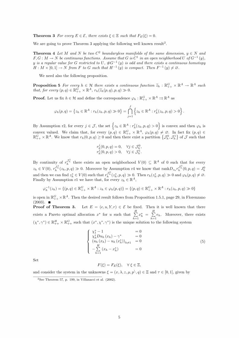
Theorem 3 For every E ∈ E, there exists ξ ∈ Ξ such that FE(ξ) = 0.

We are going to prove Theorem 3 applying the following well known result2.

Theorem 4 Let M and N be two C2 boundaryless manifolds of the same dimension, y ∈ N andF,G : M → N be continuous functions. Assume that G is C1 in an open neighborhood U of G−1 (y),y is a regular value for G restricted to U , #G−1 (y) is odd and there exists a continuous homotopyH : M × [0, 1]→ N from F to G such that H−1 (y) is compact. Then F−1 (y) 6= ∅.

We need also the following proposition.

Proposition 5 For every h ∈ H there exists a continuous function zh : RG++ × RA → RA suchthat, for every (p, q) ∈ RG++ × RA, rh(zh(p, q), p, q)� 0.

Proof. Let us fix h ∈ H and define the correspondence ϕh : RG++ × RA ⇒ RA as

ϕh(p, q) ={zh ∈ RA : rh(zh, p, q)� 0

}=

J⋂j=1

{zh ∈ RA : rjh(zh, p, q) > 0

}.

By Assumption r2, for every j ∈ J , the set{zh ∈ RA : rjh(zh, p, q) > 0

}is convex and then ϕh is

convex valued. We claim that, for every (p, q) ∈ RG++ × RA, ϕh(p, q) 6= ∅. In fact fix (p, q) ∈RG++ ×RA. We know that rh(0, p, q) ≥ 0 and then there exist a partition

{J 0h ,J 1

h

}of J such that

rjh(0, p, q) = 0, ∀j ∈ J 0h ,

rjh(0, p, q) > 0, ∀j ∈ J 1h .

By continuity of rJ1h

h there exists an open neighborhood V (0) ⊆ RA of 0 such that for every

zh ∈ V (0), rJ1h

h (zh, p, q) � 0. Moreover by Assumption r4 we know that rankDzhrJ 0

h

h (0, p, q) = J0h

and then we can find z∗h ∈ V (0) such that rJ0h

h (z∗h, p, q)� 0. Then rh(z∗h, p, q)� 0 and ϕh(p, q) 6= ∅.Finally by Assumption r1 we have that, for every zh ∈ RA,

ϕ−1h (zh) = {(p, q) ∈ RG++ × RA : zh ∈ ϕh(p, q)} = {(p, q) ∈ RG++ × RA : rh(zh, p, q)� 0}

is open in RG++×RA. Then the desired result follows from Proposition 1.5.1, page 29, in Florenzano(2003).Proof of Theorem 3. Let E = (e, u, Y, r) ∈ E be fixed. Then it is well known that there

exists a Pareto optimal allocation x∗ for u such thatH∑h=1

x∗h =H∑h=1

eh. Moreover, there exists

(χ∗, γ∗) ∈ RH++ × RG++ such that (x∗, χ∗, γ∗) is the unique solution to the following systemχ∗1 − 1 = 0χ∗hDuh (xh)− γ∗ = 0(uh (xh)− uh (x∗h))h6=1 = 0

−H∑h=1

(xh − x∗h) = 0

(5)

SetF (ξ) = FE(ξ), ∀ ξ ∈ Ξ,

and consider the system in the unknowns ξ = (x, λ, z, µ, p\, q) ∈ Ξ and τ ∈ [0, 1], given by

2See Theorem 57, p. 199, in Villanacci et al. (2002).

5

(h.1.s)h∈H,s∈S

Dxh(s)uh (xh)− λh (s) p (s) = 0

(h.2.0)h∈H

−p (0) (xh (0)− ((1− τ) eh(0) + τx∗h(0)))− qzh = 0

(h.2.s)h∈H,s∈S\{0}

−p (s) (xh (s)− ((1− τ) eh(s) + τx∗h(s))) + y (s) zh = 0

(h.3.a)h∈H,a∈A

−λh (0) qa +S∑s=1

λh (s) ya(s) +J∑j=1

µjh (1− τ)Dzahrjh ((1− τ) zh + τ zh(p, q), p, q) = 0

(h.4.j)h∈H,j∈J

min{µjh, r

jh ((1− τ) zh + τ zh(p, q), p, q)

}= 0

(M.x)H∑h=1

(x\h −

((1− τ) e\h + τx

∗\h

))= 0

(M.z)H∑h=1

zh = 0

(6)where, for every h ∈ H, the function zh is defined in Proposition 5.

Define nowH : Ξ× [0, 1]→ Rdim Ξ

(ξ, τ) 7→ left hand side of system (6),

andG : Ξ→ Rdim Ξ, ξ 7→ H (ξ, 1) .

Observe thatH (ξ, 0) = F (ξ) .

Let us now verify that Theorem 4 can be applied. F and G are defined in the same open subset ofRdim Ξ, take values in Rdim Ξ (and those sets are C2 boundaryless manifolds of the same dimension)and are continuous.

Of course H is a continuous homotopy from F to G. Moreover, Lemmas 6, 7 and 8 prove thefollowing needed results.

• G−1 (0) = {ξ∗};

• G is C1 in a neighborhood of ξ∗ and rankDξG (ξ∗) = dim Ξ;

• H−1 (0) is compact.

From Theorem 4, it then follows, as desired, that F−1(0) 6= ∅.

Lemma 6 G−1 (0) = {ξ∗} ={

(x∗, z∗, λ∗, µ∗, p\∗, q∗)}∈ Ξ, where

x∗h = x∗h, λ∗h =(γ∗C (s)χ∗h

, s ∈ S), z∗h = 0, µ∗h = 0, ∀h ∈ H,

p∗\ =(γ∗c (s)γ∗C (s)

, s ∈ S, c 6= C

), q∗ =

S∑s=1

(γ∗C (s)γ∗C (0)

)y (s) .

6

Proof. G−1 (0) is the set of solutions of system (6) at τ = 1, that is, the set of solutions of thesystem

(h.1.s)h∈H,s∈S

Dxh(s)uh (xh)− λh (s) p (s) = 0

(h.2.0)h∈H

−p (0) (xh (0)− x∗h (0))− qzh = 0

(h.2.s)h∈H,s∈S\{0}

−p (s) (xh (s)− x∗h (s)) + y (s) zh = 0

(h.3.a)h∈H,a∈A

−λh (0) qa +S∑s=1

λh (s) ya(s) = 0

(h.4.j)h∈H,j∈J

µjh = 0

(M.x)H∑h=1

(x\h − x

∗\h

)= 0

(M.z)H∑h=1

zh = 0

(7)

Using the definition of ξ∗, it is easy to check that ξ∗ ∈ G−1 (0). Define now ξ =(x, λ, z, µ, p\, q

),

assume ξ ∈ G−1(0) and prove ξ = ξ∗.Claim 1. µ = µ∗. Obvious.Claim 2. x = x∗. Suppose by contradiction x 6= x∗. Consider x = 1

2 (x+ x∗). Of course it is

H∑h=1

xh =12

(H∑h=1

xh +H∑h=1

x∗h

)=

H∑h=1

x∗h. (8)

Since (x∗h, z∗h) is feasible for the maximization problem of the h-th household, whose first order

conditions are given by equations (h.1.s), (h.2.0), (h.2.s) and (h.3.a) in (7), it is uh(xh) ≥ uh(x∗h).Moreover, from Assumption u3, we have

uh (xh) > min{uh (x∗h) , uh(xh)} = uh (x∗h) ∀h ∈ H. (9)

But (8) and (9) contradict the Pareto optimality of x∗.Claim 3. λ = λ∗. Since x = x∗, from (h.1.s) in (7) we have in particular

λh (s) = DxCh (s)uh (xh) = DxC

h (s)uh (x∗h) = λ∗h (s) , ∀h ∈ H, s ∈ S.

Claim 4. p\ = p\∗. ¿From (h.1.s) in (7) and Claims 2 and 3,

p (s) =Dxh(s)uh (xh)

λh (s)=Dxh(s)uh (x∗h)

λ∗h (s)= p∗ (s) ∀s ∈ S.

Claim 5. z = z∗. From (h.2.s) s ≥ 1 , in (7) and Claim 2, we have in particular,

Y zh = 0, ∀h ∈ H.

From Assumption Y, we get that for any h ∈ H, zh = 0 = z∗h.Claim 6. q = q∗. From (h.3.a) in (7) and Claims 1 and 3 we get

q =S∑s=1

λh (s)

λh (0)y (s) =

S∑s=1

λ∗h (s)λ∗h (0)

y (s) = q∗,

and the proof is completed.

Lemma 7 G is C1 in a neighborhood of ξ∗ and rankDξG (ξ∗) = dim Ξ.

7

Proof. It is immediate to prove that in a suitable small neighborhood of ξ∗ we have is

G(ξ) =

(h.1.s)h∈H,s∈S

Dxh(s)uh (xh)− λh (s) p (s)

(h.2.0)h∈H

−p (0) (xh (0)− x∗h (0))− qzh

(h.2.s)h∈H,s∈S\{0}

−p (s) (xh (s)− x∗h (s)) + y (s) zh

(h.3.a)h∈H,a∈A

−λh (0) qa +S∑s=1

λh (s) ya(s)

(h.4.j)h∈H,j∈J

µjh

(M.x)H∑h=1

(x\h − x

∗\h

)(M.z)

H∑h=1

zh

and this is a C1 function. The computation of DξG (ξ∗) is described below

xh λh zh µh p\ q

(h.1) D2uh (x∗h) −Φ (p∗)T −Λ∗h(h.2) −Φ (p∗)

[−q∗Y

](h.3)

[−q∗Y

]T−λ∗h (0) I

(h.4) I

(M.x) I(M.z) I

where

Φ (p) =

p1 (0) . . . pC−1 (0) 1. . .

p1 (S) ... pC−1 (S) 1

(S+1)×G

(10)

I =

I(C−1)×(C−1)0

. . .I(C−1)×(C−1)0

[G−(S+1)]×G

(11)

and

Λ∗h =

λ∗h (0) IC−1

0. . .

λ∗h (S) IC−1

0

=1χ∗h

γ∗C (0) IC−1

0. . .

γ∗C (S) IC−1

0

=1χ∗h

Γ∗,

(12)where Λ∗h and Γ∗ have G rows and G− (S + 1) columns and Γ∗ does not depend on h.

Then the above matrix has full rank if and only if the following does:

xh λh zh p\ q

(h.1) D2uh (x∗h) −Φ (p∗)T −Λ∗h(h.2) −Φ (p∗)

[−q∗Y

](h.3)

[−q∗Y

]T−λ∗h (0) I

(M.x) I(M.z) I

8

Using a standard argument exploiting Assumption u3, the desired result follows3.

Lemma 8 H−1 (0) is compact.

Proof. We want to show that any sequence(ξ[k], τ [k]

)k∈N included in H−1 (0) admits a convergent

subsequence inside that set.Since

{τ [k]}k∈N ⊆ [0, 1], up to a subsequence, we can assume τ [k] → τ ∈ [0, 1]. Consequently,

definede

[k]h =

(1− τ [k]

)eh + τ [k]x∗h, eh = (1− τ) eh + τx∗h,

e[k] =(1− τ [k]

)e+ τ [k]x∗, e = (1− τ) e+ τx∗,

we have e[k]h , eh ∈ RG++, e[k], e ∈ RGH++ and

e[k]h → eh, e[k] → e as k →∞.

Claim 1.(x[k])k∈N admits a subsequence converging to x ∈ RGH++ .

It suffices to show that(x[k])k∈N is contained in a compact subset of RGH included in RGH++ . Since{

x[k]}k∈N ⊆ RGH++ is bounded from below from zero. Observing that Walras’ law holds also for the

homotopy system, we have

H∑h=1

(x

[k]h −

((1− τ [k]

)eh + τ [k]x∗h

))= 0

and then for any h′ ∈ H

x[k]h′ =

H∑h=1

((1− τ [k]

)e

[k]h + τ [k]x∗h

)−∑h6=h′

x[k]h .

Therefore, since(e

[k]h

)k∈N

converges and(x[k])k∈N is bounded from below, it is bounded from above

as well. We are left with showing the closedness. Remember that equations (h.1.s), (h.2.0), (h.2.s),(h.3.a) and (h.4.j) in (6) say that for all k ∈ N,

(x

[k]h , z

[k]h

)solves the problem

max(xh,zh)

uh(xh) s.t.

−p[k] (0)(xh (0)− (1− τ [k])eh (0)− τ [k]x∗h(0)

)− q[k]zh = 0,

−p[k] (s)(xh (s)− (1− τ [k])eh (s)− τ [k]x∗h(s)

)+ y (s) zh = 0, s ∈ {1, ..., S}

rh((1− τ [k])zh + τ [k]zh(p[k], q[k]), p[k], q[k]

)≥ 0.

(13)

From Assumption u3 and the properties of zh it is simple to prove that, for all k ∈ N, we have thatthe vector

(e

[k]h , 0

)belongs to the constraint set described in (13), and therefore by definition of

x[k]h , we have that

uh

(x

[k]h

)≥ uh

(e

[k]h

)≥ mineh∈

ne[k]h

ok∈N∪{beh}

uh (eh) = uh, ∀k ∈ N, h ∈ H,

where the minimum is well defined because {e[k]h }k∈N∪{eh} is a compact set. Therefore,

{x[k]}k∈N ⊆{

xh ∈ RG++ : uh (xh) ≥ uh}

, which is a closed set in RG and contained in RG++ from Assumption u4.Therefore,

{x[k]}k∈N is contained in a closed set, too. We can assume then, up to a subsequence

that x[k] → x ∈ RGH++ as k →∞.

Claim 2.(λ[k])k∈N admits a subsequence converging to λ ∈ R(S+1)H

++ .Since p[k]C(s) = 1, from (h.1.s) in (6), we have

DxCh (s)uh

(x

[k]h

)= λ

[k]h (s), ∀h ∈ H, s ∈ S.

3See Villanacci et al. (2002), Lemma 18, p. 319.

9

Letting k →∞ in both sides, we get

limk→∞

λ[k]h (s) = lim

k→∞DxC

h (s)uh

(x

[k]h

)= DxC

h (s)uh (xh) = λh(s) > 0

where the last strict inequality comes from Assumption u2.

Claim 3.(p\[k]

)k∈N admits a subsequence converging to p\ ∈ RG−(S+1)

++ .

Again from (h.1.s) in (6), Dx\h(s)

uh

(x

[k]h

)− λ[k]

h (s)p\(s) = 0. Therefore, we get

limk→∞

p\[k](s) = limk→∞

Dx\h(s)

uh

(x

[k]h

)λ

[k]h (s)

=Dx\h(s)

uh (xh)

λh(s)= p\ > 0

where again the last strict inequality comes from Assumption u2.

Claim 4.(z[k])∞k=1

admits a subsequence converging to z ∈ RAH .

From equation (h.2.s) s ≥ 1 in (6), and using the fact that Y has full rank A and the previousclaims, we also get that

(z[k])∞k=1

converges.

Claim 5.(q[k])∞k=1

admits a subsequence converging to q ∈ RA.From the previous claims we know that, up to a subsequence,

(z[k], p\[k]

)converges to

(z, p\

). Let

us fix now a ∈ A and prove qa[k] → qa. From Assumption r5 there exists h ∈ H such that

(zh, p, q) ∈ RA × RG++ × RA ⇒ Dzahrh(zh, p, q) = 0

and therefore for every k we get

Dzahrh

((1− τ [k])z[k]

h + τ [k]zh(p[k], q[k]), p[k], q[k])

= 0

Then, (h.3.a) in (6) can be written as

−λ[k]h (0) qa[k] +

S∑s=1

λ[k]h (s) ya(s) = 0

and then

qa[k] =

S∑s=1

λ[k]h (s)y(s)

λ[k]h (0)

→

S∑s=1

λh(s)y(s)

λh(0)= qa.

Claim 6.(µ[k])k∈N admits a subsequence converging to µ ∈ RJH .

Fix h ∈ H and let{J 0h ,J 1

h

}be a partition of the set of indexes J such that

J 0h =

{j ∈ J : rjh

((1− τ) zh + τ zh(p, q), p, q

)= 0}

andJ 1h =

{j ∈ J : rjh

((1− τ) zh + τ zh(p, q), p, q

)> 0}

with cardinality J0h and J1

h, respectively. If j ∈ J 1h , if k is large enough it is

rjh

((1− τ [k]

)z

[k]h + τ [k]zh(p[k], q[k]), p[k], q[k]

)> 0

which implies µj,[k]h = 0. Then µ

j,[k]h → 0 as k →∞, for all j ∈ J 1

h .From Assumption r4,

rank(Dzh

rJ 0

h

h

((1− τ) zh + τ zh(p, q), p, q

))= J0

h.

10

Then∣∣detM

(zh, p

\, q, τ)∣∣ > 0 , where M

(zh, p

\, q, τ)

is a well chosen square J0h-dimensional sub-

matrix ofDzh

rJ 0

h

h

((1− τ) zh + τ zh(p, q), p, q

).

Let M(z

[k]h , p\[k], q[k], τ [k]

)be the square sub-matrix of

DzhrJ 0

h

h

((1− τ [k]

)z

[k]h + τ [k]zh(p[k], q[k]), p[k], q[k]

)(14)

whose columns are the same than the ones of M(zh, p

\, q, τ). Of course

M(z

[k]h , p\[k], q[k], τ [k]

)→M

(zh, p

\, q, τ)

;

if k is large enough we have also∣∣∣detM

(z

[k]h , p\[k], q[k], τ [k]

)∣∣∣ > 0 and then

M−1(z

[k]h , p\[k], q[k], τ [k]

)→M−1

(zh, p

\, q, τ).

Making the needed permutations of rows and columns of (14) in order to haveM(z

[k]h , p\[k], q[k], τ [k]

)in the top-left corner we get

J0h A− J0

h

J0h M

(z

[k]h , p\[k], q[k], τ [k]

)M12

(z

[k]h , p\[k], q[k], τ [k]

)J − J0

h M21

(z

[k]h , p\[k], q[k], τ [k]

)M22

(z

[k]h , p\[k], q[k], τ [k]

)Performing analogous permutation of the components of µh and η =

(−λh

[−qY

])in order to have

the equalities in equations (h.3.a), of (6) still satisfied we get:

[µ

0,[k]h µ

1,[k]h

] (1− τ [k]

) M(z

[k]h , p\[k], q[k], τ [k]

)M12

(z

[k]h , p\[k], q[k], τ [k]

)M21

(z

[k]h , p\[k], q[k], τ [k]

)M22

(z

[k]h , p\[k], q[k], τ [k]

) =[ηI,[k] ηII,[k]

]where µ0,[k]

h ∈ RJ0h , µ

1,[k]h ∈ RJ−J0

h , ηI,[k] ∈ RJ0h , ηII,[k] ∈ RA−J0

h .

Since µ1,[k]h = 0, we have in particular

µ0,[k]h

(1− τ [k]

) [M(z

[k]h , p\[k], q[k], τ [k]

)]= ηI,[k]

and thenµ

0,[k]h = ηI,[k]

[M(z

[k]h , p\[k], q[k], τ [k]

)]−1

which implies µ0,[k]h → µ0

h as k →∞ because the left hand side does converge.

4 Existence when some households cannot trade some assets

Let us consider an economy E ∈ E . For every h ∈ H let us define the set Ah ⊆ A such that, forevery a ∈ Ah,

Dzahrh(zh, p, q) = 0, ∀ (zh, p, q) ∈ RA × RG++ × RA.

Of course it may be Ah = ∅ but, because of Assumption r5, surely we have⋃h∈H

Ah = A.

Let us define then the set B(E) ⊆(2A)H as follows.4 Given B = (Bh)h∈H ∈

(2A)H we have

B ∈ B(E) if4We denote by 2A the power set of A.

11

1. for every h ∈ H, Bh ⊆ Ah,

2. for every a ∈ A, there exists h ∈ H such that a ∈ Ah \ Bh.

Moreover, for every h ∈ H, let Bh = #(Bh) and B =∑h∈HBh.

For given (p, q, E) ∈ RG++ × RA × E and B ∈ B(E), household h ∈ H maximization problem isnow as follows.

Problem (Ph2)

max(xh,zh)

uh(xh) s.t.

p (0)xh (0) + qzh ≤ p (0) eh (0)

p (s)xh (s)− pC (s) y (s) zh ≤ p (s) eh (s) , s ∈ {1, ..., S}

rh(zh, p, q) ≥ 0

zah = 0, a ∈ Bh

(15)

Moreover the definition of equilibrium is as follows.

Definition 9((xh, zh)h∈H , p, q

)∈(RG++ × RA

)H × RG++ × RA = Θ is an equilibrium for theeconomy E ∈ E and for B ∈ B(E) if for each h, (xh, zh) solves Problem (Ph2) at (p, q, E) and(x, z) solves market clearing conditions at e

H∑h=1

(xh − eh) = 0

H∑h=1

zh = 0(16)

In the following, for every E ∈ E and B ∈ B(E) we denote by Θ(E,B) ⊆ Θ the set of equilibria forthe economy E and for B ∈ B(E) by Θn(E,B) the set of normalized equilibria, that is,

Θn(E,B) ={(

(xh, zh)h∈H , p, q)∈ Θ(E,B) : ∀s ∈ S, pC(s) = 1

}.

The following existence theorem hold.

Theorem 10 For every E ∈ E and for every B ∈ B(E), Θn(E,B) 6= ∅.

The proof of Theorem 10 follows the same lines that the one of Theorem 2. In fact for this newkind of equilibria S + 1 Walras’ laws hold too and then the significant market clearing conditionsare given by (3).

Consider then E ∈ E and B ∈ B(E) as fixed and define

Ξ = RGH++ × RAH × R(S+1)H++ × RJH × RB × RG−(S+1)

++ × RA

with generic element

ξ =(

(xh, zh, λh, µh, βh)Hh=1 , p\, q)

=(x, z, λ, µ, β, p\, q

),

where, for every h ∈ H, βh ∈ RBh .It is immediate to prove that if(

(xh, zh)Hh=1 , p, q)∈ Θn(E,B)

then there exists (λ, µ, β) ∈ R(S+1)H++ × RJH × RB such that

ξ =(

(xh, zh, λh, µh, βh)Hh=1 , p\, q)

12

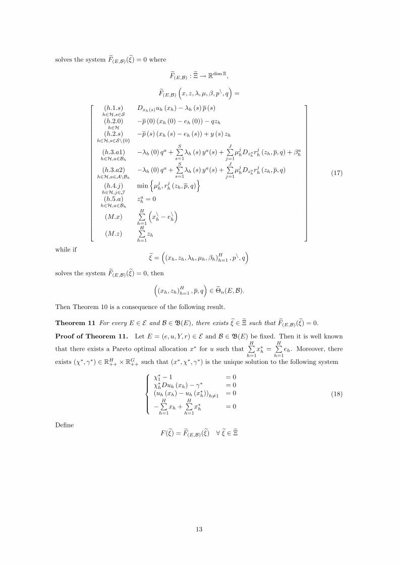
solves the system F(E,B)(ξ) = 0 where

F(E,B) : Ξ→ Rdim Ξ,

F(E,B)

(x, z, λ, µ, β, p\, q

)=

(h.1.s)h∈H,s∈S

Dxh(s)uh (xh)− λh (s) p (s)

(h.2.0)h∈H

−p (0) (xh (0)− eh (0))− qzh

(h.2.s)h∈H,s∈S\{0}

−p (s) (xh (s)− eh (s)) + y (s) zh

(h.3.a1)h∈H,a∈Bh

−λh (0) qa +S∑s=1

λh (s) ya(s) +J∑j=1

µjhDzahrjh (zh, p, q) + βah

(h.3.a2)h∈H,a∈A\Bh

−λh (0) qa +S∑s=1

λh (s) ya(s) +J∑j=1

µjhDzahrjh (zh, p, q)

(h.4.j)h∈H,j∈J

min{µjh, r

jh (zh, p, q)

}(h.5.a)h∈H,a∈Bh

zah = 0

(M.x)H∑h=1

(x\h − e

\h

)(M.z)

H∑h=1

zh

(17)

while ifξ =

((xh, zh, λh, µh, βh)Hh=1 , p

\, q)

solves the system F(E,B)(ξ) = 0, then((xh, zh)Hh=1 , p, q

)∈ Θn(E,B).

Then Theorem 10 is a consequence of the following result.

Theorem 11 For every E ∈ E and B ∈ B(E), there exists ξ ∈ Ξ such that F(E,B)(ξ) = 0.

Proof of Theorem 11. Let E = (e, u, Y, r) ∈ E and B ∈ B(E) be fixed. Then it is well known

that there exists a Pareto optimal allocation x∗ for u such thatH∑h=1

x∗h =H∑h=1

eh. Moreover, there

exists (χ∗, γ∗) ∈ RH++ × RG++ such that (x∗, χ∗, γ∗) is the unique solution to the following systemχ∗1 − 1 = 0χ∗hDuh (xh)− γ∗ = 0(uh (xh)− uh (x∗h))h6=1 = 0

−H∑h=1

xh +H∑h=1

x∗h = 0

(18)

DefineF (ξ) = F(E,B)(ξ) ∀ ξ ∈ Ξ

13

and consider the system in the unknowns ξ = (x, λ, z, µ, β, p\, q) ∈ Ξ and τ ∈ [0, 1] given by

(h.1.s)h∈H,s∈S

Dxh(s)uh (xh)− λh (s) p (s) = 0

(h.2.0)h∈H

−p (0) (xh (0)− ((1− τ) eh(0) + τx∗h(0)))− qzh = 0

(h.2.s)h∈H,s∈S\{0}

−p (s) (xh (s)− ((1− τ) eh(s) + τx∗h(s))) + y (s) zh = 0

(h.3.a1)h∈H,a∈Bh

−λh (0) qa +S∑s=1

λh (s) ya(s) +J∑j=1

µjh(1− τ)Dzahrjh ((1− τ) zh + τ zh(p, q), p, q) + βah = 0

(h.3.a2)h∈H,a∈A\Bh

−λh (0) qa +S∑s=1

λh (s) ya(s) +J∑j=1

µjh(1− τ)Dzahrjh ((1− τ) zh + τ zh(p, q), p, q) = 0

(h.4.j)h∈H,j∈J

min{µjh, r

jh ((1− τ) zh + τ zh(p, q), p, q)

}= 0

(h.5.a)h∈H,a∈Bh

zah = 0

(M.x)H∑h=1

(x\h − e

\h

)= 0

(M.z)H∑h=1

zh = 0

(19)where, for every h ∈ H, the function zh is defined in Proposition 5.

Define nowH : Ξ× [0, 1]→ Rdim eΞ(

ξ, τ)7→ left hand side of system (19),

andG : Ξ→ Rdim eΞ, ξ 7→ H

(ξ, 1).

Observe thatH(ξ, 0)

= F(ξ).

Let us now verify that Theorem 4 can be applied. F and G are defined in the same open subset ofRdim eΞ, take values in Rdim eΞ (and those sets are C2 boundaryless manifolds of the same dimension)and are continuous.

Of course H is a continuous homotopy from F to G. Moreover, Lemmas 12, 13 and 14 provethe following needed results.

• G−1 (0) ={ξ∗}

;

• G is C1 in a neighborhood of ξ∗ and rankDeξG(ξ∗)

= dim Ξ;

• H−1 (0) is compact.

From Theorem 4, it then follows, as desired, that F−1(0) 6= ∅.

Lemma 12 G−1 (0) ={ξ∗}

={

(x∗, z∗, λ∗, µ∗, β∗, p\∗, q∗)}∈ Ξ, where

x∗h = x∗h, λ∗h =(γ∗C (s)χ∗h

, s ∈ S), z∗h = 0, µ∗h = 0, β∗h = 0 ∀h ∈ H,

p∗\ =(γ∗c (s)γ∗C (s)

, s ∈ S, c 6= C

), q∗ =

S∑s=1

(γ∗C (s)γ∗C (0)

)y (s) .

14

Proof. G−1 (0) is the set of solutions of system (19) at τ = 1, that is, the set of solution of thesystem

(h.1.s)h∈H,s∈S

Dxh(s)uh (xh)− λh (s) p (s) = 0

(h.2.0)h∈H

−p (0) (xh (0)− x∗h(0))− qzh = 0

(h.2.s)h∈H,s∈S\{0}

−p (s) (xh (s)− x∗h(s)) + y (s) zh = 0

(h.3.a1)h∈H,a∈Bh

−λh (0) qa +S∑s=1

λh (s) ya(s) + βah = 0

(h.3.a2)h∈H,a∈A\Bh

−λh (0) qa +S∑s=1

λh (s) ya(s) = 0

(h.4.j)h∈H,j∈J

µjh = 0

(h.5.a)h∈H,a∈Bh

zah = 0

(M.x)H∑h=1

(x\h − e

\h

)= 0

(M.z)H∑h=1

zh = 0

(20)

Using the definition of ξ∗, it is easy to check that ξ∗ ∈ G−1 (0). Define now ξ =(x, λ, z, µ, β, p\, q

)and assume ξ ∈ G−1(0): we prove ξ = ξ∗.Claim 1. µ = µ∗. Obvious.Claim 2. x = x∗. Suppose by contradiction x 6= x∗. Consider x = 1

2 (x+ x∗). Of course it is

H∑h=1

xh =12

(H∑h=1

xh +H∑h=1

x∗h

)=

H∑h=1

x∗h. (21)

Since (x∗h, z∗h) is feasible for the maximization problem of the h-th household, whose first order

conditions are given by equations (h.1.s), (h.2.0), (h.2.s), (h.3.a1), (h.3.a2) and (h.5.a) in (20), itis uh(xh) ≥ uh(x∗h). Moreover, from Assumption u3, we have

uh (xh) > min{uh (x∗h) , uh(xh)} = uh (x∗h) ∀h ∈ H. (22)

But (21) and (22) contradict the Pareto optimality of x∗.Claim 3. λ = λ∗. Since x = x∗, from (h.1.s) in (20) we have in particular

λh (s) = DxCh (s)uh (xh) = DxC

h (s)uh (x∗h) = λ∗h (s) , ∀h ∈ H, s ∈ S.

Claim 4. p\ = p\∗. From (h.1.s) in (20) and Claims 2 and 3,

p (s) =Dxh(s)uh (xh)

λh (s)=Dxh(s)uh (x∗h)

λ∗h (s)= p∗ (s) ∀s ∈ S.

Claim 5. z = z∗. From (h.2.s) s ≥ 1, in (20) and Claim 2, we have in particular,

Y zh = 0, ∀h ∈ H.

From Assumption Y, we get that for any h ∈ H, zh = 0 = z∗h.Claim 6. q = q∗. From the assumption on B and (h.3.a2) in (20), for every a ∈ A, there existsh ∈ H

qa =S∑s=1

λh (s)

λh (0)ya (s) =

S∑s=1

λ∗h (s)λ∗h (0)

ya (s) = qa∗,

Claim 7. β = β∗. From (h.3.a1) in (20) and Claims 1 and 6 we get the claim and the proof is nowcompleted.

Lemma 13 G is C1 in a neighborhood of ξ∗ and rankDeξG(ξ∗)

= dim Ξ.

15

Proof. It is immediate to prove that in a suitable small neighborhood of ξ∗ we have

G(ξ) =

(h.1.s)h∈H,s∈S

Dxh(s)uh (xh)− λh (s) p (s)

(h.2.0)h∈H

−p (0) (xh (0)− x∗h(0))− qzh

(h.2.s)h∈H,s∈S\{0}

−p (s) (xh (s)− x∗h(s)) + y (s) zh

(h.3.a1)h∈H,a∈Bh

−λh (0) qa +S∑s=1

λh (s) ya(s) + βah

(h.3.a2)h∈H,a∈A\Bh

−λh (0) qa +S∑s=1

λh (s) ya(s)

(h.4.j)h∈H,j∈J

µjh

(h.5.a)h∈H,a∈Bh

zah

(M.x)H∑h=1

(x\h − e

\h

)(M.z)

H∑h=1

zh

and this is a C1 function. The computation of DeξG

(ξ∗)

is described below

xh λh zh µh βh p\ q

(h.1) D2uh (x∗h) −Φ (p∗)T −Λ∗h(h.2) −Φ (p∗)

[−q∗Y

](h.3)

[−q∗Y

]TIBh

−λ∗h (0) I

(h.4) I

(h.5) ITBh

(M.x) I(M.z) I

where Φ (p), I, Λ∗h are defined in (10), (11) and (12) respectively, and if Bh = {b1, . . . , bBh}, with

b1 < . . . < bBh, then

IBh= (γi,j)

j=1,...,Bh

i=1,...,A where γi,j ={

1 if i = bj0 if i 6= bj

The above matrix has full rank if and only if the following does:

M∗ =

xh λh zh βh p\ q

(h.1) D2uh (x∗h) −Φ (p∗)T −Λ∗h(h.2) −Φ (p∗)

[−q∗Y

](h.3)

[−q∗Y

]TIBh

−λ∗h (0) I

(h.5) ITBh

(M.x) I(M.z) I

(23)

We are going to use a simple modification of the standard argument. Consider a vector

∆ξ =(

(∆xh,∆zh,∆λh,∆µh,∆βh)Hh=1 ,∆p\,∆q

)

16

and prove that if M∆ξ = 0 then ∆ξ = 0. Let us explicitly write M∆ξ = 0 as follows:

(h.1) D2uh (x∗h) ∆xh − Φ (p∗)T ∆λh − Λ∗h∆p\ = 0(h.2) −Φ (p∗) ∆xh +

[−q∗Y

]∆zh = 0

(h.3)[−q∗Y

]T∆λh + IBh

∆βh − λ∗h (0) ∆q = 0

(h.5) ITBh∆zh = 0

(M.x)H∑h=1

∆x\h = 0

(M.z)H∑h=1

∆zh = 0

(24)

and remember that, from (20) we have in particular{(h.1) Duh (x∗h)− λ∗hΦ (p∗) = 0

(h.3)[−q∗Y

]Tλ∗h = 0

(25)

First we claim that if, for every h ∈ H, ∆xh = 0 then ∆ξ = 0. In fact if, for every h ∈ H, ∆xh = 0then, from (h.2) in (24) we have [

−q∗

Y

]∆zh = 0,

and from Assumption Y we have ∆zh = 0. From (h.1) in (24) it follows ∆λh = 0 that implies∆p\ = 0 as well. From (h.3) in (24) we obtain the equality

IBh∆βh = λ∗h (0) ∆q.

We know that, for every a ∈ A, there exists h ∈ H such that a ∈ Ah \ Bh. Then we have that, forevery a ∈ A, ∆qa = 0 that is ∆q = 0. As a consequence we have that, for every h ∈ H, ∆βh = 0too and the proof of the claim is complete.

Let us assume now there exists h′ ∈ H such that ∆x′h 6= 0 and prove that this leads to acontradiction. First of all let us show that, for every h ∈ H, Duh(x∗h)∆xh = 0. In fact multiplying(h.1) in (25) by ∆xh, for every h ∈ H, we obtain

Duh (x∗h) ∆xh = λ∗hΦ (p∗) ∆xh.

From (h.2) in (24) we have

Duh (x∗h) ∆xh = λ∗h

[−q∗

Y

]∆zh

and the right hand side is zero because of (h.3) in (25). The claim then follows and since ∆xh′ 6= 0and Assumption u3 holds, we have in particular that

H∑h=1

χ∗h∆xhD2uh(x∗h)∆xh < 0. (26)

We end the proof of the lemma showing that it has also to be

H∑h=1

χ∗h∆xhD2uh(x∗h)∆xh = 0, (27)

and then finding a contradiction.From (h.1) in (24) we have

χ∗h∆xhD2uh(x∗h)∆xh = χ∗h∆xhΦ (p∗)T ∆λh + χ∗h∆xhΛ∗h∆p\.

Moreover from (h.2) and (h.3) in (24) we have

χ∗h∆xhΦ (p∗)T ∆λh = χ∗h∆zh

[−q∗

Y

]T∆λh = ∆zh

(γ∗C(0)∆q − χ∗hIBh

∆βh).

17

and by definition of Λ∗h and Γ∗ we have

χ∗h∆xhΛ∗h∆p\ = ∆xhΓ∗∆p\.

Then

H∑h=1

χ∗h∆xhD2uh(x∗h)∆xh =

(H∑h=1

∆zh

)γ∗C(0)∆q −

H∑h=1

χ∗h∆zhIBh∆βh +

(H∑h=1

∆xh

)Γ∗∆p\.

We are going to prove (27) showing then the right hand side of the above equality is zero. Of courseby (M.z) in (24) (

H∑h=1

∆zh

)γ∗C(0)∆q = 0.

Moreover we have (H∑h=1

∆xh

)Γ∗∆p\ =

(H∑h=1

∆x\h,H∑h=1

∆xCh

)Γ∗∆p\ = 0

using (M.x) in (24) and the properties of Γ∗. Finally from (h.5) in (24) we have

H∑h=1

χ∗h∆zhIBh∆βh = 0

and the proof is completed.

Lemma 14 H−1 (0) is compact.

Proof. We want to show that any sequence(ξ[k], τ [k]

)k∈N included in H−1 (0) admits a convergent

subsequence inside that set.Since

{τ [k]}k∈N ⊆ [0, 1], up to a subsequence, we can assume τ [k] → τ ∈ [0, 1]. Consequently,

definede

[k]h =

(1− τ [k]

)eh + τ [k]x∗h, eh = (1− τ) eh + τx∗h,

e[k] =(1− τ [k]

)e+ τ [k]x∗, e = (1− τ) e+ τx∗,

we have e[k]h , eh ∈ RG++, e[k], e ∈ RGH++ and

e[k]h → eh, e[k] → e as k →∞.

Claim 1.(x[k])k∈N admits a subsequence converging to x ∈ RGH++ .

It suffices to show that(x[k])k∈N is contained in a compact subset of RGH included in RGH++ . Since{

x[k]}k∈N ⊆ RGH++ is bounded from below from zero. Observing that Walras’ law holds also for the

homotopy system, we have

H∑h=1

(x

[k]h −

((1− τ [k]

)eh + τ [k]x∗h

))= 0

and then for any h′ ∈ H

x[k]h′ =

H∑h=1

((1− τ [k]

)e

[k]h + τ [k]x∗h

)−∑h6=h′

x[k]h .

Therefore, since(e

[k]h

)k∈N

converges and(x[k])k∈N is bounded from below, it is bounded from above

as well. We are left with showing the closedness. Remember that equations (h.1.s), (h.2.0), (h.2.s),

18

(h.3.a1), (h.3.a2), (h.4.j) and (h.5.a) in (19) say that for all k ∈ N,(x

[k]h , z

[k]h

)solves the problem

max(xh,zh)

uh(xh) s.t.

−p[k] (0)(xh (0)− (1− τ [k])eh (0)− τ [k]x∗h(0)

)− q[k]zh = 0,

−p[k] (s)(xh (s)− (1− τ [k])eh (s)− τ [k]x∗h(s)

)+ y (s) zh = 0, s = 1, ..., S

rh((1− τ [k])zh + τ [k]zh(p[k], q[k]), p[k], q[k]

)≥ 0

zah = 0, a ∈ Bh

(28)

From Assumption u3 and the properties of zh it is simple to prove that, for all k ∈ N, we have thatthe vector

(e

[k]h , 0

)belongs to the constraint defined by (28), and therefore by definition of x[k]

h , wehave that

uh

(x

[k]h

)≥ uh

(e

[k]h

)≥ mineh∈

ne[k]h

ok∈N∪{beh}

uh (eh) = uh, ∀k ∈ N, h ∈ H,

where the minimum is well defined because {e[k]h }k∈N∪{eh} is a compact set. Therefore,

{x[k]}k∈N ⊆{

xh ∈ RG++ : uh (xh) ≥ uh}

, which is a closed set in RG and contained in RG++ from Assumption u4.Therefore,

{x[k]}k∈N is contained in a closed set, too. We can assume then, up to a subsequence

that x[k] → x ∈ RGH++ as k →∞.

Claim 2.(λ[k])k∈N admits a subsequence converging to λ ∈ R(S+1)H

++ .See Claim 2 of the proof of Lemma 8.

Claim 3.(p\[k]

)k∈N admits a subsequence converging to p\ ∈ RG−(S+1)

++ .See Claim 3 of the proof of Lemma 8.

Claim 4.(z[k])∞k=1

admits a subsequence converging to z ∈ RAH .See Claim 4 of the proof of Lemma 8.

Claim 5.(q[k])∞k=1

admits a subsequence converging to q ∈ RA.From the previous claims we know that, up to a subsequence,

(z[k], p\[k]

)converges to

(z, p\

). Let

us fix now a ∈ A and prove qa[k] → qa. From Assumption r5 and the properties of B we know thereexists h ∈ H such that a ∈ Ah \ Bh and therefore, for every k, we get

Dzahrh

((1− τ [k])z[k]

h + τ [k]zh(p[k], q[k]), p[k], q[k])

= 0

Then, (h.3.a2) in (19) can be written as

−λ[k]h (0) qa[k] +

S∑s=1

λ[k]h (s) ya(s) = 0

and then

qa[k] =

S∑s=1

λ[k]h (s)y(s)

λ[k]h (0)

→

S∑s=1

λh(s)y(s)

λh(0)= qa.

Claim 6.(µ[k])k∈N admits a subsequence converging to µ ∈ RJH .

See Claim 6 of the proof of Lemma 8.

Claim 7.(β[k])k∈N admits a subsequence converging to β ∈ RB.

It immediately follows from (h.3.a1) in (19) and the already proved claims. The proof of the lemmais then completed.

19

References

Carosi L, Gori M, Villanacci A. Endogenous restricted participation in general financial equilib-rium, mimeo, 2009.

Cass D, Siconolfi P, Villanacci A. Generic Regularity of Competitive Equilibria with RestrictedParticipation, Journal of Mathematical Economics 2001; 36; 61-76.

Florenzano, M., General Equilibrium Analysis. Kluwer Academic Press, 2003.

Villanacci A, Carosi L, Benevieri P, Battinelli A. Differential Topology and General Equilibriumwith Complete and Incomplete Markets, Kluwer Academic Publishers, 2002.

20