UNIVERSITA DEGLI STUDI DI PADOVA ...
68
UNIVERSIT ` A DEGLI STUDI DI PADOVA Dipartimento di Fisica ed Astronomia “Galileo Galilei” Corso di Laurea Magistrale in Fisica Efimov bound states in polymer physics Relatore: Candidata: Dott. Antonio Trovato Federica Mura Correlatore: Prof. Flavio Seno Anno Accademico 2013/2014
Transcript of UNIVERSITA DEGLI STUDI DI PADOVA ...

UNIVERSITA DEGLI STUDI DI PADOVA
Dipartimento di Fisica ed Astronomia “Galileo Galilei”
Corso di Laurea Magistrale in Fisica
Efimov bound states in polymer physics
Relatore: Candidata:
Dott. Antonio Trovato Federica Mura
Correlatore:
Prof. Flavio Seno
Anno Accademico 2013/2014


Abstract
The aim of this thesis is to investigate, using simplified lattice models, whetherthe Efimov effect, well known in quantum mechanics, can arise in polymerphysics too, particularly in a triple stranded DNA system. Such effect con-sists in the formation of stable trimer bound states when dimer bound statesare not stable.We base strand interaction rules on a Poland-Scheraga model for a directedDNA-like polymer, double-stranded first and triple-stranded later. Within thePoland-Scheraga scheme, only interactions between base pairs with the samemonomer indexes along the strands are permitted. Thus, the identificationof the monomer index with imaginary time allows the formal mapping to thequantum problem in which particles interact at the same time. According tothe transfer matrix method, we are able to extract information about the free-energy of the system from matrix eigenvalues. Studying them at the criticalpoint of the unzipped-zipped phase transition we look for the similarities be-tween the bound states in the polymer model and those predicted by Efimovtheory for a three particle quantum system. In particular, in Efimov theory,an infinite series of trimer energy levels, with a constant ratio between con-secutive levels, is found at the critical point of the 2-body problem.In chapter 1 we briefly describe the main characteristics of double strandedDNA physical and chemical structure, triple stranded DNA and the denatu-ration process which will be the main arguments of this work.In chapter 2 we give an elementary explanation of the Efimov effect in quan-tum physics concentrating on the conditions for which the effect arises. Wealso explain why to expect that an analogue of the Efimov effect could takeplace in a polymer system.In the third chapter we give an analytic procedure to solve exactly the twostrands DNA system. After that, we define the Poland-Scheraga model ona 1+1 directed lattice and we introduce the transfer matrix method for thetwo chain system, starting from a recursive equation for the partition functioncomputed on the lattice. We see how the matrix eigenvalues are related to thefree energy of the system and then to the phase transition in the denatura-tion process. The results achieved in this chapter also act as a check of suchmethod on a problem that is analytically solvable.In chapter 4 we face the task to build up the transfer matrix for the morecomplex three stranded system, then in chapter 5 we table the achieved re-sults in comparison with those of the double stranded system. In particular weobserve a shift between the transition point of the three and two chain system,accompanied by a free energy variation, in agreement with the analogy sug-gested by the quantum case. On the other hand, we do not find any evidencefor the existence of the analogy with the infinite series of Efimov trimers.


Contents
1 Introduction 1
1.1 DNA structure . . . . . . . . . . . . . . . . . . . . . . . . . . . 21.2 Triple stranded DNA . . . . . . . . . . . . . . . . . . . . . . . . 31.3 DNA denaturation . . . . . . . . . . . . . . . . . . . . . . . . . 61.4 DNA and random walks . . . . . . . . . . . . . . . . . . . . . . 7
2 Efimov states 9
2.1 Two body problem . . . . . . . . . . . . . . . . . . . . . . . . . 92.1.1 Two-body scattering at low energy . . . . . . . . . . . . 92.1.2 Separable two-body potential . . . . . . . . . . . . . . . 11
2.2 Efimov spectrum and the inverse square potential . . . . . . . . 122.3 The three body problem . . . . . . . . . . . . . . . . . . . . . . 132.4 Efimov effect in polymer physics . . . . . . . . . . . . . . . . . 15
3 Double chain DNA models 19
3.1 Generating function . . . . . . . . . . . . . . . . . . . . . . . . 193.1.1 Directed lattice model . . . . . . . . . . . . . . . . . . . 21
3.2 Transfer matrix method . . . . . . . . . . . . . . . . . . . . . . 233.2.1 Free energy from the transfer matrix method . . . . . . 263.2.2 Numerical results . . . . . . . . . . . . . . . . . . . . . . 273.2.3 Transfer matrix eigenvectors . . . . . . . . . . . . . . . 303.2.4 Mathematical notes . . . . . . . . . . . . . . . . . . . . 33
4 Triple chain DNA models 37
4.1 Three chains in a cylinder . . . . . . . . . . . . . . . . . . . . . 38
5 Results and discussion 47
5.1 Extrapolation . . . . . . . . . . . . . . . . . . . . . . . . . . . . 495.2 Eigenvectors . . . . . . . . . . . . . . . . . . . . . . . . . . . . . 54
6 Conclusions and future perspectives 57
iii


CONTENTS
Acknowledgements
I would like to sincerely thanks all those who helped me in this work, withopinions, corrections, critics and encouragements, that were fundamental forme from the beginning to the end.Firstly my supervisor Dott. Antonio Trovato of having involved me in thisproject and led constantly, giving most of his time and meeting me every timeI need. I am also grateful to my co-supervisor Prof. Flavio Seno, even ifthere were few occasions to work with him directly, I know that he has alwaysbeen interested in shaping this thesis and willing to give us his co-operationand opinion. My thanks also go to Giovanni who helped me, instead of beingin England, and to Hicham who adjusted the terrible English that I used towrite these acknowledgements. Last but not least, I wish to give thanks toStefano, not only for the unique practical and moral support he has given mein this thesis period, but also for everything that he has taught me during thisacademic path, with his sympathy also during his most challenging period,making always available his aptitude for giving me answers to my too manyand infinite questions.
v


Chapter 1
Introduction
Deoxyribonucleic acid, more commonly known as DNA, is a complex moleculethat contains all the information necessary to build and maintain living organ-isms. However, DNA does more than specifying the structure and function ofliving systems things, it also serves as the primary unit of heredity in organ-isms of all types. In other words, whenever organisms reproduce, a portionof their DNA is passed along to their offspring. This transmission of all orpart of an organism’s DNA helps ensure a certain level of continuity from onegeneration to the next, while still allowing for slight changes that contributeto the diversity of life.The discovery of DNA double-helical structure by Watson, Crick, Wilkins andFranklin in 1953 [11] was an important milestone of modern biology. Theyobserved that DNA is formed by two complementary strands where, throughhydrogen bonds, an adenine pairs with thymine, and guanine with cytosineforming A-T and G-C base pairs. The succession of base pairs defines the ge-netic information and gives the information to the cell to accomplish its vitalfunctions.Four years later, Felsenfeld et al [9] found that in DNA there are acceptor anddonor groups that can form hydrogen bond interactions with a third strand.This was the starting point for a number of studies that have had great impactin medical progress, for example with the development of the Antigen Ther-apy [5], based on gene silencing approach. This technique delivers short, singlestranded pieces of DNA, called oligonucleotides, that bind specifically betweena gene’s two DNA strands. This binding makes a triple-helix structure thatblocks the DNA from being transcribed into mRNA.Of course, a good model is a fine starting point to understand the implica-tions and the potential of the triple helix structure. Since DNA is a polymerformed by a great number of monomers it is reasonable to describe it with amechanical statistical approach, and this is what we are going to do in this
1

CHAPTER 1. Introduction
work with particular interest in the three chains structure.Firstly, we need a clear understanding of the biological structure of doubleand triple helical, in order to decide how to build our statistical model.
1.1 DNA structure
DNA in the form proposed for the first time by Watson and Crick is a longpolymer, made from repeated units called nucleotides. The basic structurecomprises two helical chains of nucleotides each coiled round the same axis,and each with a pitch of 34 angstroms (A, 1 A= 0.1 nm) and a radius of 10A. When measured in a particular solution, the DNA chain measured 22 to26 A in width, and one nucleotide unit measured 3.3 A long [18]. Althougheach individual repeating unit is very small, DNA polymers can be very largemolecules containing millions of nucleotides. For instance, the largest humanchromosome, chromosome number 1, consists of approximately 220 millionbase pairs and would be 85 mm long, if completely stretched.
Figure 1.1: A section of DNA.
Each nucleotide consists of a 5-carbon sugar (deoxyribose), a nitrogen con-taining base attached to the sugar, and a phosphate group. There are fourdifferent types of nucleotides found in DNA, differing only in the nitrogenousbase. The four nucleotides are given one letter abbreviations as shorthand forthe four bases: adenine (A), guanine (G), cytosine (C), thymine (T). Adenineand guanine are purines (5 carbon, 4 nitrogen) that are the largest of the twotypes of bases found in DNA, while thymine and cytosine are pyrimidines (4carbon, 2 nitrogen).The deoxyribose sugar of the DNA backbone has 5 carbons and 3 oxygens.The carbon atoms are numbered 1’, 2’, 3’, 4’, and 5’ to distinguish from thenumbering of the atoms of the purine and pyrmidine rings. Along the single
2

1.2 – Triple stranded DNA
strand each phosphate group binds the 3’-carbon of a deoxyribose moleculewith the 5’-carbon of the sequent sugar, forming phosphodiester bonds.In a double stranded DNA (dsDNA), each type of nucleobase on one strandpairs with just one type of nucleobase on the other strand. This is calledcomplementary base pairing. Here, purines form hydrogen bonds with pyrim-idines, with adenine bonding only to thymine with two hydrogen bonds, andcytosine bonding only to guanine with three hydrogen bonds.
Figure 1.2: DNA chemical structure.
Moreover the double helical structure is stabilised not only by hydrogenbonds, but also by the hydrophobic effect and especially by van der Waalsinteractions between parallel bases, also known as base stacking interactions,characterized by cooperativity.
1.2 Triple stranded DNA
Triple-stranded DNA (tsDNA) is a structure of DNA in which three oligonu-cleotides wind around each other and form a triple helix. Triplex formationis governed by sequence-specific binding rules that are conceptually similar
3

CHAPTER 1. Introduction
to the familiar Watson-Crick base-pairing rules. The third nucleotide strandbinds to dsDNA through Hoogsteen or reversed Hoogsteen hydrogen bonds[10].In the Hoogsteen pairing the adenine base is flipped as compared to Watson-Crick pairing and, since one nucleotide side is connected to one helix and theother is connected to the other helix, that’s going to change the shape of thatportion of the DNA. In Fig.(1.3) are shown the two possible Hoogsteen pairsfor the TAT couple or CGC.
Thymine
Adenine
Thymine
Cytosine
Guanine
Cytosine
T ∗A− T C ∗G− C
Figure 1.3: TAT and CGC pairing in tsDNA. The symbol ∗ indicate the Hoogsteenbase pairs and the − the Watson-Crick base pairs
Moreover the Hoogsteen pairing is stable only in determinate contexts,as pH 5 or lower, and the G-C Watson-Crick pairing consists of one morehydrogen bond than Hoogsteen pairing. Indeed normally, the Watson-Crickstructure is favoured over the Hoogsteen scheme.Besides the TAT and CGC pairing in the tsDNA also the GGC and AAT arepermitted. In these last cases the Hoogsteen pairing G*G and A*A is said tobe reverse because the purines sugars are located in the opposite side com-pared to the first case.The central strand in tsDNA have to be formed by purines only, because thepyrimidines cannot have multiple hydrogen bonds on both sides simultane-ously.Two particular types of tsDNA have been identified:
• the intermolecular tsDNA, discovered in 1957, formed between triplexforming oligonucleotides (TFO) consisting in a single DNA strand thatbinds to a target sequences on duplex DNA.
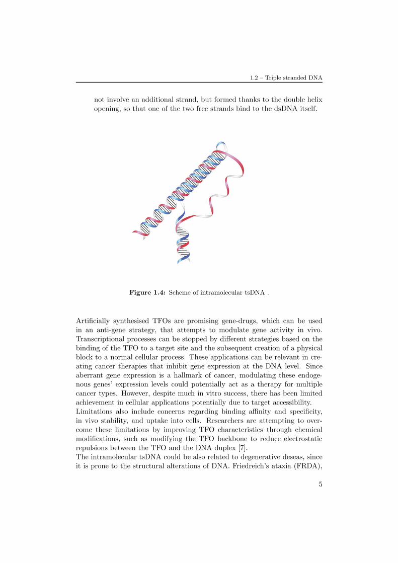
• the intramolecular tsDNA (Fig.(1.4)), discovered in 1987 [23], that does
4
1.2 – Triple stranded DNA
not involve an additional strand, but formed thanks to the double helixopening, so that one of the two free strands bind to the dsDNA itself.
Figure 1.4: Scheme of intramolecular tsDNA .
Artificially synthesised TFOs are promising gene-drugs, which can be usedin an anti-gene strategy, that attempts to modulate gene activity in vivo.Transcriptional processes can be stopped by different strategies based on thebinding of the TFO to a target site and the subsequent creation of a physicalblock to a normal cellular process. These applications can be relevant in cre-ating cancer therapies that inhibit gene expression at the DNA level. Sinceaberrant gene expression is a hallmark of cancer, modulating these endoge-nous genes’ expression levels could potentially act as a therapy for multiplecancer types. However, despite much in vitro success, there has been limitedachievement in cellular applications potentially due to target accessibility.Limitations also include concerns regarding binding affinity and specificity,in vivo stability, and uptake into cells. Researchers are attempting to over-come these limitations by improving TFO characteristics through chemicalmodifications, such as modifying the TFO backbone to reduce electrostaticrepulsions between the TFO and the DNA duplex [7].The intramolecular tsDNA could be also related to degenerative deseas, sinceit is prone to the structural alterations of DNA. Friedreich’s ataxia (FRDA),
5

CHAPTER 1. Introduction
the autosomal recessive degenerative disorder of nervous and muscles tissuecaused by the transcriptional silencing of the FXN gene, is the only diseaseknown so far to be associated with DNA triplex [25].
1.3 DNA denaturation
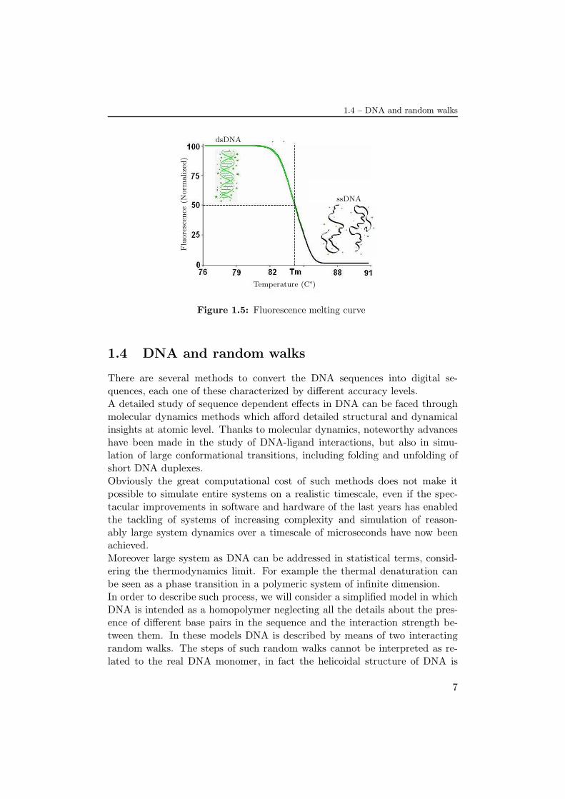
The hydrogen bonds between bases of different strands are not covalent sothat they can be broken and reformed relatively easily. The two strands ofDNA in a double helix can therefore be pulled apart like a zipper, either bya mechanical force or temperature increase. When DNA is destabilised bytemperature, the process is called melting, and occurs at high temperature,low salt and high pH. However low pH also melts DNA, but since DNA isunstable in this context, low pH is rarely used.Since the base pair A-T forms two hydrogen bonds and G-C three, the G-Cbase pair is stronger so that the dsDNA stability depends on the GC-content.Other indicators for stability are the sequence, because the stacking is se-quence specific, and the length, because long molecules are more stable. Acommon way to measure the stability is the melting temperature Tmc, whichis the temperature at which 50% of the nucleotides are converted from theclose (folded) to the open (unfolded) state.The primary experimental tool for studying the denaturation process is themeasurement of UV light absorption at a wavelength of about 270 nm. Lightat this wavelength is preferentially absorbed by the single strands and it thusprovides a measure for the fraction of the double-stranded pairs, θ(T), at anygiven temperature T. This is known as the optical melting curve of the DNA.We expects θ to decrease with temperature and to vanish at very high temper-ature[21]. This kind of analysis required µg amounts of DNA, and often tookhours to complete. Contemporary DNA melting analysis uses fluorescencebecause it is a more sensitive method. It needs only ng amounts of DNA,shortening the melting time to a few minutes. (Fig.(1.5))The denaturation process is energetically disadvantaged (Ess−Eds = ∆E > 0)because of the hydrogen bonds, while is entropically favoured (Sss−Sds=∆S >0) because the single strands are more flexible over the double strands so thatthe spatial configurations are more numerous for the denatured DNA. Indeedthe transition occurs when the system reaches a particular temperature abovewhich the free energy variation Fss−Fds = ∆F = ∆E−T∆S became negative.
6
1.4 – DNA and random walks
Temperature (C°)
dsDNA
ssDNA
Fluorescen
ce(N
orm
alized)
Figure 1.5: Fluorescence melting curve
1.4 DNA and random walks
There are several methods to convert the DNA sequences into digital se-quences, each one of these characterized by different accuracy levels.A detailed study of sequence dependent effects in DNA can be faced throughmolecular dynamics methods which afford detailed structural and dynamicalinsights at atomic level. Thanks to molecular dynamics, noteworthy advanceshave been made in the study of DNA-ligand interactions, but also in simu-lation of large conformational transitions, including folding and unfolding ofshort DNA duplexes.Obviously the great computational cost of such methods does not make itpossible to simulate entire systems on a realistic timescale, even if the spec-tacular improvements in software and hardware of the last years has enabledthe tackling of systems of increasing complexity and simulation of reason-ably large system dynamics over a timescale of microseconds have now beenachieved.Moreover large system as DNA can be addressed in statistical terms, consid-ering the thermodynamics limit. For example the thermal denaturation canbe seen as a phase transition in a polymeric system of infinite dimension.In order to describe such process, we will consider a simplified model in whichDNA is intended as a homopolymer neglecting all the details about the pres-ence of different base pairs in the sequence and the interaction strength be-tween them. In these models DNA is described by means of two interactingrandom walks. The steps of such random walks cannot be interpreted as re-lated to the real DNA monomer, in fact the helicoidal structure of DNA is
7

CHAPTER 1. Introduction
stiff because subsequent monomers are constrained to maintain a fixed anglebetween them for chemical reasons. We can interpret the random walk modelas an equivalent polymer in which each monomer is formed by a set of differ-ent nucleotides. This model is known as Equivalent freely jointed chain andconsist in a coarse graining of the real model of DNA strands.Another fundamental aspect to consider in DNA modellisation is the excludedvolume effect. Experimental studies on DNA melting are always carried on insolution and a property of a good solvent is that interaction of the polymerwith solvent molecules is energetically favoured over interaction with othermonomers. Indeed each monomer is surrounded by solvent molecules, formingan inaccessible region for the other chain elements. The most common wayto describe such effect is the self-avoiding walk (SAW), that is a model inwhich self-intersection in the chain paths are banned. The Poland-Scheragamodel that we are going to introduce in the Ch.(3) involve two different SAW,representing dsDNA, of which only elements with the same distance from theorigin, measured along the strands, can interact. This option is useful to ap-proximate the DNA base pairing and will enable us to develop an analogy withthe quantum case of two interacting particles. In fact is possible to interpretthe step index in the random walks as the time parameter in the quantumproblem in which particles can interact only at the same time.
8

Chapter 2
Efimov states
The Efimov effect is an effect in quantum mechanics first predicted by V.Efimov in 1970 [28] for identical bosons that occupy a spatially symmetrics-state and interact with a short-range pair-wise potential.In these circumstances, their spectrum obeys a geometrical scaling law, suchthat the ratio of the successive energy eigenvalues of the system is a constantand accumulation of states near zero energy takes place. When the dimerbinding is zero and the two-body state is exactly at the dissociation threshold,the number of three-body bound states is infinite. Indeed, three body boundstates are stable when two-body ones not. An issue to emphasise is the factthat Efimov effect is independent of the details of the interaction, for example,whether it is between atoms with a pair-wise van der Waals interaction, orbetween nuclei with a nuclear force.In 2005, for the first time the research group of Rudolf Grimm and Hanns-Christoph Nagerl from the Institute for Experimental Physics (University ofInnsbruck, Austria) experimentally confirmed such a state in an ultracold gasof caesium atoms [16]. At such low temperatures (10 nK) thermal motion doesnot mask quantum effects.In this chapter an elementary exposition of the Efimov effect, will be givenusing basic concepts of quantum mechanics.
2.1 Two body problem
2.1.1 Two-body scattering at low energy
We need to recall the most important results about the quantum mechanicalproblem of a beam of particles incident at low energy upon a target. In princi-ple, if we assume that all the in-going particles are represented by wavepacketsof the same shape and size, our challenge is to solve the full time-dependent
9

CHAPTER 2. Efimov states
Schrodinger equation for such a wavepacket
ih∂tΨ(r, t) =
[
− h2
2m∇2 + V (r)
]
Ψ(r, t) (2.1)
and find the probability amplitudes for out-going waves in different directionsat some later time after scattering has taken place. However, if the incidentbeam of particles is switched on for times very long as compared with the timea particle would take to cross the interaction region, steady-state conditionsapply. Moreover, if we assume that the incident wavepacket has a well-definedenergy (and hence momentum), so it is many wavelengths long, we may con-sider it a plane wave. Setting Ψ(r, t) = ψ(r)e−iEt/h we may therefore look forsolutions ψ(r) of the time-independent Schrodinger equation
Eψ(r) =
[
− h2
2m∇2 + V (r)
]
ψ(r) (2.2)
subject to the boundary condition that the incoming component of the wave-function is a plane wave, eik·x. Here E = p2/2m = h2k2/2m denotes theenergy of the incoming particles.In the three-dimensional system the wavefunction well outside the localizedtarget region will involve a superposition of the incident plane wave and thescattered spherical wave
ψ(r) ≃ eik·r + f(θ)eikr
r(2.3)
where we assume that the potential perturbation V (r) depends only on theradial coordinate and the function f(θ) records the relative amplitude andphase of the scattered components along the direction θ relative to the incidentbeam.Using the partial wave method the wavefunction can be expanded in a seriesof Legendre polynomials and f(θ) results
f(θ) =
∞∑
l=0
(2l + 1)fl(k)Pl(cos θ) (2.4)
where Pl(cos θ) denote the Legendre Polynomials and fl(k) is the partial wavescattering amplitude. At low energies is possible to show that the total scat-tering amplitude is dominated by the s-wave (l = 0) channel and results
f(θ) ≃ f0(k) = (k cot δ0(k)− ik)−1 (2.5)
10

2.1 – Two body problem
where δ0(k) is the s-wave phase shift caused by potential. The scatteringbetween the two particles is well described [12] at low energies by two shape-independent parameters, the scattering length a and the effective range r0,where
k cot δ0(k) = −1
a+
1
2r0k
2 + . . . (2.6)
The scattering length a is linked to potential strength and for a square well
potential, considering h = 2m = 1, a =(
1− tanγγ
)
with γ = U1/20 R , U0
the depth and R the width of well potential. At low energies, k → 0, thescattering cross-section, σ = 4πa2 is fixed by the scattering length alone. Ifγ ≪ 1, a is negative. As γ is increased, when γ = π/2, both a and σ diverge- there is said to be a zero energy resonance. This condition corresponds toa potential well that is just able to support an s-wave bound state. We’ll seethat the Efimov effect arise in this context.
2.1.2 Separable two-body potential
Consider the scattering of a heavy particle of mass M interacting with a lightone of mass m, with the mass ratio ρ = M
m . The relative energy is given byE2 = k2/ν ′ where we have set again h = 2m = 1 and ν ′ = ρ/(ρ + 1). Forsimplicity we assume ρ≫ 1 and ν ′ = 1. The eigenvalues equation is
(
k2 −H0
)
|ψk〉 = V |ψk〉 (2.7)
where H0 is the kinetic energy operator. The Eq.(2.7) takes the form
(
k2 +∇2)
ψk(r) =
∫
〈r|V |r′〉ψk(r′)d3r′ (2.8)
in the r-space with r the relative coordinate between the two particles, and
(
k2 − p2)
ψk(p) =
∫
〈p|V |p′〉ψk(p′)d3p′ (2.9)
in the p-space, where p is the relative momentum between the two particles.A separable potential in Hilbert space may be written as V = −λ |g〉 〈g|, wherethe negative sign is taken for attraction, and λ > 0 determines the strengthof the potential. In the coordinate representation the separable potential inr-space is given by 〈r|V |r〉 = −λg(r)g(r′) where g(r) is taken to be real. TheSchrodinger equation in p-space for a bound state k2 = −k20 is given by
(k20 + p2)ψk0(p) = λg(p)
∫
g(p′)ψk0(p′)d3p′ (2.10)
11

CHAPTER 2. Efimov states
where
g(p) =
∫
〈p|r〉g(r)d3r = 1
(2π)3/2
∫
exp(−ip · r)g(r)d3r (2.11)
Rewriting Eq.(2.10) as
ψk0(p) = λCk0
g(p)
(k20 + p2)(2.12)
with Ck0 =∫
g(p′)ψk0(p′)d3p′ and multiplying both sides by g(p) and integrat-
ing over d3p we obtain the equation that determines the binding energy k20 fora given potential
λ
∫
g(p)2
(k20 + p2)d3p = 1 (2.13)
For explicit calculations we choose the popular Yamaguchi form g(p) = (p2 +β2)−1 giving
g(r) =1
(2π)3/2
∫
exp(ip · r)g(p)d3p =√
π
2
exp(−βr)r
(2.14)
and
ψk0(r) = λCk0
√
π
2
(
exp(−k0r)r
− exp(−βr)r
)
(2.15)
2.2 Efimov spectrum and the inverse square poten-
tial
Let us now focus upon the problem of a single particle of mass m in an inversesquare potential V (r) = (h2/2m)λ′/r2 where λ′ is a dimensionless couplingconstant.It’s possible to show that for λ′ > −1/4 there is no bound states, while infiniteand continuous number of bound states arise for λ′ < −1/4. In order to solvethis problem we need to take a short distance cut-off in some point r = rc andimpose that eigenfunctions vanish on it [27][6].We are interested in the situation where the potential is inverse square onlyfor r > rc so we can write the radial (u(r) = rψ(r)) Schrodinger equation forthis case:
[
− d2
dr2− s20 + 1/4
r2
]
u(r) =2m
h2Eu(r) (2.16)
where s20 ≥ 0 is just a way of parametrizing the strength of an inverse squarepotential whose coupling constant is smaller than −1/4. For bound states, we
12

2.3 – The three body problem
set (2m/h2)E = −k2, and require that wave functions vanish at infinity. Thisequation give us an energy spectrum for shallow bound states that follows ageometric scaling law given by [13] :
En+1
En= exp(−2π/s0) n = 0, 1, 2, ...∞ (2.17)
Note that as n becomes larger, the states become shallower, with an infinitenumber of states accumulating at zero energy. This results will be useful, aswe’ll see in due course, to solve in the three body problem the Schrodingerequation for radial coordinate.
2.3 The three body problem
Our aim is now to obtain an inverse square interaction, like that of the previoussection, in the three body problem where the particles interact with a shortrange pair-wise potential. This objective is best served by taking two identicalheavy particles 1 and 2, each of mass M, and particle 3 of mass m ≪ M .The analysis is simplified if the relative coordinates R = (r1 − r2) and r =r3 − (r1 + r2)/2 are introduced, where r1, r2 and r3 are the coordinates ofparticles 1, 2 and 3 measured from an arbitrary origin. Following the commonconvention, we denote by V1 the interparticle potential between particles 2and 3, and likewise for V2 and V3 in cyclic order. The Schrodinger equationresults
HΨ(r,R) = EΨ(r,R) (2.18)
with
H = − 1
µ∇2
R −1
ν∇2
r + V1(r−R/2) + V2(r+R/2) + V3(R) (2.19)
µ = ρ/2 ν = 2ρ/(2ρ + 1) (2.20)
where E is the total energy of the system and ρ = M/m, recalling thath = 2m = 1. For ρ ≫ 1, ν → 1, and the motion of the heavy particles isvery slow compared to that of the light particle of mass m, so that we canapply the adiabatic Born-Oppenheimer approximation to solve the three-bodySchrodinger equation in two stages. First, the wave function is decomposedaccording to
Ψ(r,R) = ψ(r,R)φ(R) (2.21)
where ψ(r,R) with eigenenergy ǫ(R), is first solved for the relative motion ofthe light-heavy system, keeping R as parameter. For fixed R the relative ki-netic energy of the heavy particle is zero, and the potential V3(R) is a constant
13

CHAPTER 2. Efimov states
shift in energy and can be neglected at this stage. Eq.(2.18) becomes
[
−∇2r + V1(r−R/2) + V2(r+R/2)
]
ψ(r,R) = ǫ(R)ψ(r,R) (2.22)
Next, we can solve within the adiabatic approximation the two-body Schrodingerequation with ǫ(R) as the adiabatic potential between the two heavy particles
[−∇2R/µ+ V3(R) + ǫ(R)]φ(R) = Eφ(R) (2.23)
For V1 and V2 in Eq.(2.22), we take the short-range separable potential −λ |g〉 〈g|.Thus for a fixed parameter R we have
〈r′ −R/2|V1 |r−R/2〉 = −λ〈r′ −R/2|g〉〈g|r −R/2〉 (2.24)
〈r′ +R/2|V2 |r+R/2〉 = −λ〈r′ +R/2|g〉〈g|r +R/2〉 (2.25)
In the p-space after some algebra and letting ǫ(R) = −k2(R) the Eq.(2.22)takes the form
λ
∫
g2(pr)
p2r + k2d3pr + λ
∫
g2(pr)exp(ipr ·R)
p2r + k2d3pr = 1 (2.26)
The coupling constant λ may be eliminated by relating it to the binding k20of the two body problem from Eq.(2.13). For the Yamaguchi form g(p) =(p2 + β2)−1 the integrals in Eq(2.26) may be performed analytically, giving
1−(
β + k0β + k
)2
=
(
β + k0β + k
)2 [ 2β
(β − k)2e−kR − e−βR
R− β + k
β − ke−βR
]
(2.27)
As the distance R between the two heavy atoms is increased, the light atomtend to attach to one of them, and k2(R)→ k20. We are particularly interestedin this large R behaviour of ǫ(R) as the two-body binding k20 goes to zero. It’sconvenient to define ζ ≡ k−k0 and substitute it into Eq.(2.27). In the resonantlimit, consider a → +∞ so that k0 = 1/a → 0 [13], and moreover k0 ≪ β,βR ≫ 1, R/a → 0, ζ ≪ β so that exp(−βR) → 0 and exp(−k0R) → 1. TheEq.(2.27) in this limit results
e−ζR
ζR= 1 (2.28)
which has the solution ζR = A where A = 0.5671 . . . Hence k = k0 + ζ =k0 + A/R. In the resonant limit we see that ǫ(R) = −k2 = −A2/R2, givingthe desired inverse square potential.In our analysis, we set ν = 1, which only approximately holds for ρ ≫ 1.However, setting ν = 1 is not necessary, but it’s possible to show [1] thatǫ(R) = −µA2/(νR2) = −(1/4A2)(1 + 2ρ)/R2. Substituting this expression in
14

2.4 – Efimov effect in polymer physics
E = 0
a < 0 a > 0
1/aEnergy
Figure 2.1: Bound and unbound states for three and two particles system. Thebound Efimov states are shown schematically by solid lines, with a scaling factor setartificially at 2 rather than 22.7. We see that for a < 0, even though there is no twobody bound state (dimer), more three-body bound states (trimers) are formed. Fora > 0 the trimers break up at the atom-dimer continuum, indicated by the dottedcurve.
Eq.(2.23) and neglecting the short-range potential V3 we obtain an equationsimilar in form to that achieved in the previous section for single particle inan inverse square potential.Indeed Efimov spectrum arise in three body problem too, and the scalingparameter s0 depends on the mass ratio ρ. For three identical bosons weget exp(π/s0) ≃ 22.694 . . .. The number of shallow bound states is givenapproximately by [1]
N ≃ s0π
ln|a|r0
(2.29)
and we note that it diverges in the resonant limit a → ∞ with finite r0 fora short range potential. Fig.(2.1) depicts the Efimov scenario for the threeboson states plotted as function of 1/a.
2.4 Efimov effect in polymer physics
After seeing the underlying causes of Efimov states in quantum mechanics,we’re going to investigate whether this effect can arise in polymer physics too.To look into that, consider three Gaussian polymers interacting through aDNA base pairing type short range potential. The Hamiltonian for such sys-tem results [3]
15

CHAPTER 2. Efimov states
βH =
∫ N
0ds
3∑
j=1
Kj
2
(
∂rj(s)
∂s
)2
+∑
k<l
Vkl(rk(s), rl(s))
(2.30)
where s is the length variable measured along the contour of the chain andidentify the monomer, j is the index of the chain (j = 1, 2, 3), rj(s) is themonomer position, Vkl is the short-range attractive interaction between chainsk and l, Kj is a bending rigidity controlling the flexibility of chain j.We can obtain the partition function of the system by summing over (
∫
DR)all configurations of the three chains:
Z =
∫
DR exp(−βH) (2.31)
The DNA-quantum correspondence relates the quantum critical threshold tothe thermal melting of duplex DNA, a continuous transition in this modelof Gaussian chains, with a diverging length scale. Suppose that we havetwo non-interacting chains 1 and 3, both interacting with another one, chain2. For simplicity, although not essential, in the spirit of Born-Oppenheimerapproximation we may take 1 and 3 as relatively stiffer compared to 2, notingthat in Eq.(2.30) the stiffness parameter Kj in the kinetic term, takes theplace of mass of the quantum case. The system composed by chain 1 andchain 2 or chain 2 and chain 3 is characterized generally by the presence ofmany crossings which define a sequence of bubbles (Fig.2.2). These bubblesare described by two scales: ξ⊥ for the spatial extent and ξ‖ for the length ofthe bubbles along the chain. Since ξ⊥ is linked to the correlation length of thesystem and ξ‖ to the relaxation time, these are related by ξ‖ ∼ ξz⊥, where z isa size exponent for polymers. Moreover, we note that the melting transitionof double chain system takes place in the limit ξ⊥ → ∞. The diffusive orGaussian nature of the free chains for our case implies z = 2 [20]. If ξ⊥ > R,where R is the distance between chain 1 and 3, then in between two contactswith chain 1, chain 2 is expected to meet chain 3, thus mediating an effectiveinteraction between chains 1 and 3.By expliciting in the Eq(2.31) the sum over the configurations of each chainwe achieve:
Z =
∫
DR1
∫
DR2
∫
DR3 exp
[
−β∫ N
0dsK1
2
(
∂r1∂s
)2
+
+K2
2
(
∂r2∂s
)2
+K3
2
(
∂r3∂s
)2
+ V (r1, r2) + V (r2, r3) + V (r1, r3)
] (2.32)
16

2.4 – Efimov effect in polymer physics
ξ⊥ξ‖
1 2 3
s
R
Figure 2.2: Two non interacting Gaussian chains 1 and 3 separated by a distanceR. Each of these can pairs with a flexible chain 2, denoted by the thin line. Theextent along the bubble contour is ξ‖ and the spatial extent is ξ⊥,while s is the lengthvariable measured along the contour of the chain.
Born-Oppenheimer approximation allows to perform the integration over theconfigurations of flexible chain 2, fixing that of the other two chains. Theanalogy with the quantum case suggests that the outcome of such operationcould be the emergence of three chains bound states at two chains criticalpoint, resulting in a reduction of the free energy of the system. As in thequantum case the effect of the light particle induces an attractive interaction,at long length scales, between the other two particles, so in the polymer systemwe expect the arising of similar interaction between the stiffer chains.We can assume the change in free energy as:
∆F ∼ −Nξ‖f(R/ξ⊥) (2.33)
where the first factor is the numbers of bubbles and f(x) is a scaling function.In the limiting behaviour suggested by the quantum analogy, for ξ⊥ → ∞,Eq.(2.33) should be finite, requiring f(x) ∼ x−z as x → 0. Indeed, in thislimit and for z = 2 we have
ǫ(R) ≡ ∆F
N≃ − A
Rz= − A
R2(2.34)
where A is constant. We see the emergence of an inverse square interaction likein the quantum case suggesting the origin of three chain Efimov-like bound
17

CHAPTER 2. Efimov states
states. Different polymer models based on hierarchical diamond lattice orEuclidean lattice in 1+1 dimensions have been developed by Jaya Maji et
al.[20] and have given us the numerical evidence that the melting point inDNA unzipped-zipped transition is different in the case of three or two chains.Thus three chains bound states would appear to arise even if there are notwo chain bound states yet. In the next chapters we will try to find a directevidence of Efimov states in the well known Poland-Scheraga polymer modelusing the transfer matrix technique that allows us to directly access the freeenergy of a system of infinite chains confined in a finite lattice strip, eventuallyhighlighting the presence of bound states.
18

Chapter 3
Double chain DNA models
From a statistical mechanics point of view the two chain system is obviouslysimpler than that with three chains. In the latter case, many difficulties areencountered in the calculation of the partition function, so that we need analternative technique to obtain information about the system. In order to dothat, we will use the well known transfer matrix method.On the other hand different theoretical models have been developed to studythe double chains DNA configurations by a statistical mechanics approach.In this chapter we will discuss one of these models and we will see how toobtain the partition function exactly and other analytical results. This willbe helpful because it allows to compare these analytical outcomes with thoseachieved by the transfer matrix technique applied to the two chain system,testing therefore such method in this context.
3.1 Generating function
A simple but accurate way to describe DNA structure was introduced byPoland and Scheraga [4] and consists of two infinite random walks that caninteract when two point of different walks, whit the same distance from theorigin, touch each other. This is useful to simulate complementary DNA basepairing, where, to a good approximation, only bases with the same chemicaldistance from the origin can join together. Configurations of partially meltedDNA are represented in this model as alternating sequences of double strandedsegments (rods) and single stranded loops (bubble), as depicted in Fig.(3.1).To make analytical computations feasible, we shall ignore the variations inbinding energy for different nucleotides, and assign an average energy ǫ < 0per double-stranded base pair. The weight of a rod segment formed by lnucleotides is thus exp(−βǫl) = wl. We assign also a weight σ for each bubbleopening to take into account the difficulty to pass from a rod segment to the
19

CHAPTER 3. Double chain DNA models
bubble rod
Figure 3.1: Schematic representation of the Poland-Scheraga model.
bubble and the corresponding increase in free energy when two bases breakup. The parameter σ reflect the breaking of cooperative stacking interactionbetween consecutive base pairs. In real DNA σ ≃ 10−4÷10−5 and denaturatingbubbles are strongly suppressed.For the sake of simplicity we choose to start and end the DNA chain with rodsegments. We consider indeed a chain of N steps, formed by s bubbles ands+1 rods with lengths, in order of position along the chain, i0, j1, i1, . . . , js, is,where j are the lengths of the bubbles and i those of the rods. Since all internalsegments must measure one step at least, it is required that
i0 +
s∑
τ=1
(iτ + jτ ) = N, 0 ≤ s ≤[
N − 1
2
]
(3.1)
The canonical partition function results
ZN (w) =
[(N−1)/2]∑
0
∑
{iτ ,jτ}
(
s∏
τ=1
viτwiτ+1gσujτ
)
vi0(wz)i0 (3.2)
where {iτ , jτ} denotes the sum over all possible lengths of segments such thati0 +
∑
τ (iτ + jτ ) = N ; viτ is the number of different configurations of rodswith length iτ and ujτ is the number of different configurations of bubbleswith length jτ . The g factor is 2 when the crossing of two strands is allowedand 1 otherwise. In other words, we are defining bubbles for two chains thatare not allowed to cross each other in a one-dimensional system.
20
3.1 – Generating function
The grand canonical partition function, with fugacity z, is
G(w, z) =
∞∑
N=0
zNZN (w)
=
∞∑
N=0
[(N−1)/2]∑
s=0
∑
{iτ ,jτ}
(
s∏
τ=1
viτwiτ+1gσujτ z
iτ+jτ
)
vi0(wz)i0
=
∞∑
s=0
∞∑
N=2s
∑
{iτ ,jτ}
(
s∏
τ=1
viτw(wz)iτ gσujτ z
jτ
)
vi0(wz)i0
=
∞∑
s=0
s∏
τ=1
∞∑
iτ=0
∞∑
jτ=0
viτw(wz)iτ gσujτ z
jτ
∞∑
i0=0
vi0(wz)i0
=
∞∑
s=0
∞∑
i=0
∞∑
j=0
viw(wz)igσujz
j
s
·∞∑
i0=0
vi0(wz)i0
(3.3)
We define now the generating function V (x) for rods and U(x) for bubbles
V (x) =
∞∑
i=0
vixi, U(x) =
∞∑
j=0
ujxj (3.4)
Indeed we obtain
G(w, z) = V (wz)∞∑
s=0
(wgσU(z)V (wz))s =V (wz)
1−wgσU(z)V (wz)(3.5)
3.1.1 Directed lattice model
To compute explicitly the generating functions in Eq.(3.4) we introduce thePoland-Scheraga model [4] for a directed self-avoiding polymer in a 1+1 squarelattice. Particularly, consider two strands moving in oblique-lattice as showedin Fig.(3.2); at each step we enforce them to increase their coordinate alongthe (1, 1) direction so that the possibles moves need to be along (1, 0) or (0, 1)directions.
In this way self-intersections are banned and only interactions betweenbases with the same distance from the origin are permitted, as it should happenfor two complementary DNA strands.The last request is important regarding the problem of the quantum mappingin which particles interact at the same time. We can map, in fact, the N -th strand step to the N -th instant of discretized time in the formalism forquantum particles.
21

CHAPTER 3. Double chain DNA models
Figure 3.2: Double stranded polymer in oblique lattice.
These rules demand two different possibilities at each step and therefore thenumber of different paths for a rod with length i is vi = 2i and V results:
V (x) =
∞∑
i=0
2ixi =1
1− 2x(3.6)
To find an explicit expression for the bubble generating function is more com-plicated and it results [2]
U(z) =1− 2z −
√1− 4z
2(3.7)
Finally, the grand canonical partition function results
G(z, w) =1
1−2wz
1− wgσ 11−2wz
1−2z−√1−4z
2
=2
2− 4wz − wgσ(1 − 2z −√1− 4z)
(3.8)
There are two points of non analyticity for G:
• zU = 14 that is the radius of convergence of U(z)
• zc such that 2− 4wz = wgσ(1 − 2z −√1− 4z), namely
zc(w) =1
(2− gσ)2
[
2
w− gσ
(
1
w+ 1−
√
1− 2
w+gσ
w
)]
(3.9)
22
3.2 – Transfer matrix method
Since the free energy density f = F/N , where N is the steps number and Fthe total free energy, is linked to the radius of convergence rc of the grandcanonical partition function [14] by
f = limN→∞
KBT ln rc(w) (3.10)
we obtain that the denaturation transition take place at wt such that the twosingularities are equal
wt =4
2 + gσ(3.11)
We can mark that in the case of allowed crossing (g = 2) and σ = 1/2 itresults wt = 4/3.Henceforward we’ll be interested only in the case with crossing, so we set g = 2and this will the value used in the following.In this discussion we enforce the rearmost segments to join together, but ingeneral we can find configurations with open strands ending in a ”fork config-uration”. Anyhow, the generating function of fork segments don’t insert othersingularities in the partition function of the system, so that the value of w atthe transition point remains the same [24].
3.2 Transfer matrix method
An alternative form to express the canonical partition function is
ZN (w, σ) =N∑
x=0
dN (x,w, σ) (3.12)
where x is the unsigned distance between the strands at the end of the chainand dN (x,w, σ) is the partition function for all configurations with fixed x.So let’s see now how a recursive equation for dN can be achieved. The twostrands in the square lattice can move in four different ways, so that eachconfiguration with a fixed ending distance x at the N -th step can be obtainedin four different ways starting from the (N − 1)-th step: two starting fromdistance x, one from x+ 1 and another one from x− 1 (Fig.3.13).In general we should apply the relation dN (x) =
∑
x′ dN−1(x′)µ(x, x′)p(x, x′)
where µ(x, x′) is the number of ways of passing from distance x′ to distancex and p(x, x′) is the weight due to bubble opening and base pair interactionin double-stranded segments. An alternative formulation could be given ifbubble closure is weighted; the two formulations (weighting either openingor closure) yield different results for finite size, but the same results in the
23

CHAPTER 3. Double chain DNA models
b
b
b
b
b
b
b
b
b
b
= + + +x x+ 1 x− 1
Figure 3.3: Scheme of recurrence relation for the coefficients dN (x).
thermodynamic limit.Therefore, the recurrence relation for the partition function with fixed x results
dN (x) = [2dN−1(x) + dN−1(x− 1)(2σ)δx,1 + dN−1(x+ 1)]wδx,0 (3.13)
Obviously for a system in an infinite lattice the dN (x) are vectors of infinitedimension [dN (0), dN (1), ..., dN (∞)]T because all ending distances x betweenstrands are permitted. But, with appropriate periodic boundary conditions,we can confine paths in a finite strip of transverse size L and infinite length. Inthis way the dN (x) are vectors of finite dimension: [dN (0), dN (1), ..., dN (L/2)]T .In fact, if we impose the top and bottom side of the strip to coincide, the pathsare enforced to move in a cylinder of base circumference L and the largest dis-tance which can be achieved is L/2 [Fig.(3.4)].
x
Figure 3.4: Paths in a strip with periodic boundary conditions.
24

3.2 – Transfer matrix method
The boundary conditions now in place are (for the case of L even)
dN (L/2) =2dN−1(L/2) + dN−1(L/2 − 1)
dN (L/2− 1) =2dN−1(L/2 − 1) + dN−1(L/2− 2) + 2dN−1(L/2)
dN (0) =2dN−1(0)w + dN−1(1)w
dN (1) =2dN−1(1) + 2dN−1(0)σ + dN−1(2)
(3.14)
In particular when the ending distance is x = L/2, two of the four possiblemoves don’t change the distance and the other two lower it to L/2− 1.In other words we enforce reflecting boundary conditions at x = L/2 to ex-ploit the mirror symmetry x → L − x within the cylindrical strip. Similarly,reflecting boundary conditions are enforced at x = 0 because the two chainsare allowed to cross each other.Thanks to this confining it is possible to write the Eq.(3.13) in matrix form
dN (x) =
L/2∑
y=0
TxydN−1(y) (3.15)
where we have introduced the transfer matrix T, which is tridiagonal andresults
T =
2w w 02σ 2 1
1. . .
. . .. . .
. . . 1
. . .. . . 2
0 1 2
(3.16)
Considering the Eq.(3.12) and the Eq.(3.15) we obtain immediately
ZN =∑
x
TxydN−1(y)
=∑
x
TxyTymdN−2(m)
=∑
x
T 2xmTmndN−3(n) = · · ·
=∑
x
TNxl d0(l)
(3.17)
where we adopt the Einstein’s convention for the sum over the repeated in-dexes.
25

CHAPTER 3. Double chain DNA models
If in general we expand the initial state d0 as a superposition of the transfermatrix eigenvectors [v1, · · · ,vL/2], from Eq.(3.17) we obtain
ZN =∑
x
TNxl d0(l)
=∑
x
TNxl (a1v1(l) + a2v2(l) + · · ·+ aL/2vL/2(l))
=∑
x
(a1λN1 v1(x) + a2λ
N2 v2(x) + · · ·+ aL/2λ
NL/2vL/2(x))
=∑
x
λN1
(
a1v1(x) + a2
(
λ2
λ1
)Nv2(x) + · · ·+ aL/2
(
λL/2
λ1
)NvL/2(x)
)
(3.18)
3.2.1 Free energy from the transfer matrix method
A general property of the interacting system which could be described usingthe transfer matrix formalism is that thermodynamic quantities will dependon its largest eigenvalue in the thermodynamic limit.Supposing that eigenvalues are arranged in descending order, so that λ1 is thelargest one, considering the limit N →∞, in the expression that we obtainedfor the partition function only the first term survives. The free energy densityin natural units is therefore given by:
f = limN→∞
1
N(− lnZN )
≃ 1
N
(
−N lnλ1 − ln
(
∑
x
a1v1(x)
))
≃− lnλ1
(3.19)
Importantly, the free energy density depends only on the largest eigenvalue.Hence, the thermodynamic quantities which are different derivatives of the freeenergy density will also depend on λ1.The ratio between the second and the first eigenvalues influence the timeemployed by the system to reach the equilibrium ξ‖ according to
1
ξ‖= ln
(
λ1λ2
)
(3.20)
in turn related to the correlation length of the system by ξ‖ = ξz⊥, with z = 2.We expect both quantities to diverge for a phase transition, with ξ⊥ linearwith the system size.
26

3.2 – Transfer matrix method
3.2.2 Numerical results
In this section we present the main results of the transfer matrix methodapplied to the two chain model. Note that all energies and free energies val-ues given in this thesis are in unit of KBT, whereas the temperature scaleis set by w = exp(−ǫ/KBT) via the choice of the pairing energy parameterǫ ∼ −8.9 Kcal/mol [22].The analytical achievement discussed in section 3.1.1 tells us that the phasetransition point is located at w = 4/3. From Eq.(3.10) we also expect thefree energy density to be constant for w ≤ 4/3, with rc = 1/4, and start todecrease for w > 4/3 with rc given by Eq.(3.9).In Fig.(3.5) is shown, as a function of w, the free energy obtained from thelargest eigenvalue of the transfer matrix, for different values of matrix dimen-sion L/2 and compared with the expected analytical function f(w). We cansee, already for L/2 = 500, the numerical data essentially agreeing with thetheoretical prediction. The vertical dashed lines correspond to the w valuesfor which we have observed the free energy trend at varying L, as depicted inFig.(3.6). Particularly, the free energy is shown as a function of 1/(L/2), sothat the limit L→∞ can be seen in 1/(L/2)→ 0. We note that in Fig.(3.6a)and Fig.(3.6b) the limit for 1/(L/2)→ 0 is − ln 4, while in Fig.(3.6c) is ln(zc)with zc given by Eq.(3.9) computed for w = 1.34, σ = 1/2 (and g = 2).The results for unbound states below the transition at w = 4/3 can also bejustified with an entropic argument: at each step the strands have four dif-ferent possible moves, so that after N steps the entropy results S = kB ln 4N .Starting from F = U−TS and considering two non interacting strands (U = 0,σ = w = 1), the free energy density in natural units 1/kBT , becomes exactlyf = − ln 4. Since we know that for w < wt and L→∞ the free energy densitymust be constant, so it results f = − ln 4 in the entire interval [1, wt].At w = wt = 4/3, it can be shown explicitly that λ1 = 4 is an eigenvalue of thetransfer matrix of Eq.(3.16) for all L values, as indeed shown in Fig.(3.6b).In Fig.(3.7) we plot the relaxation time ξ‖, rescaled to the square systemsize, given from Eq.(3.20) and computed for different values of L/2. Recallingthat we expect ξ‖ to diverge at transition point, we note that its peak raisesat growing L, suggesting that the phase transition takes place in the limitL→∞.
27

CHAPTER 3. Double chain DNA models
1.2 1.24 1.28 1.32 1.36 1.4−1.395
−1.39
−1.385
−1.38
w
f
L/2 = 10L/2 = 20L/2 = 30L/2 = 500f(w)
Figure 3.5: Free energy, σ = 1/2
0 0.002 0.004 0.006 0.008 0.01−1,386296
−1,386292
−1,386288
−1,386284
−1,38628
−1,386276
1/(L/2)
f
lnλ1
ln4
(a) w = 1.33, σ = 1/2
28

3.2 – Transfer matrix method
0 0.002 0.004 0.006 0.008 0.01
−1,38636
−1,38632
−1,38628
−1,38624
−1,3862
1/(L/2)
f
lnλ1
ln4
(b) w = 4/3, σ = 1/2
0 0,002 0,004 0,006 0,008 0,01−1,38637
−1,38636
−1,38635
−1,38634
−1,38633
1/(L/2)
f
lnλ1
lnzc
(c) w = 1.34, σ = 1/2
Figure 3.6: L→∞ limit for different values of w.
29

CHAPTER 3. Double chain DNA models
1.32 1.324 1.328 1.332 1.336 1.340
0,1
0,2
0,3
0,4
w
ξ ‖/(L/2)2
L/2 = 200
L/2 = 300
L/2 = 400
L/2 = 500
Figure 3.7: ξ‖ rescaled to the square system size, for different values of L/2, σ = 1/2.
It is clear that the peaks of different curves in Fig.(3.7) move towards leftwhen L/2 increases, approaching the transition point of the infinite system at4/3. Therefore, we could reasonably estimate wt looking for the positions ofthe peaks at every L. To improve the precision of peak localization we havecomputed the relaxation time, at fixed L, for different w at steps of ∆w = 10−4
around the theoretical transition point. Successively, we have selected a subsetof ten points located around the maximum and interpolated with a 4th orderpolynomial. The peak of the relaxation time profile was then computed byanalytically finding the local maximum of the interpolated curve. This processwas repeated varying L/2 between 200 to 2000 and the resulting wt estimateswere plotted against 1/(L/2) in Fig.(3.8) in order to point out the L → ∞limit at 1/(L/2) = 0.
3.2.3 Transfer matrix eigenvectors
It is interesting to deal with the meaning of the transfer matrix eigenvectorsin our specific problem. From Eq.(3.18) it is evident that in the N →∞ limitthe only contribute to the partition function is given from the first eigenvectorv1 linked to the largest eigenvalue λ1. In particular the probability to have a
30

3.2 – Transfer matrix method
0 1 2 3 4 5 6
x 10−3
1.333
1.3335
1.334
1.3345
1.335
1.3355
1.336
1/(L/2)
wt
wt
4/3
Figure 3.8: Transition point wt against 1/(L/2) varying L/2 from 200 to 2000 atsteps of 100.
certain ending distance x results
P (x) =dN (x)
ZN=
a1λN1 v1(x)
∑
x a1λN1 v1(x)
=v1(x)∑
v1(x)
(3.21)
Therefore, when N → ∞ the probability distribution of ending distance xdepends on the first eigenvector components and this vector represents thestationary state of the system. This means that whatever the initial conditionmay be, the system will go to position itself in the same state. If we plotthe first eigenvector components against x (Fig.(3.9a)) or the correspondentprobability distribution P (x) (Fig.(3.9b)) for different values of w in the zippedphase (w > 4/3), we can see that, over the transition, the states of the systemwith small final distances x between strands are favoured with an exponentialdecay, reminiscent of the ground state wavefunction in a δ-function potentialwell that would be obtained in the corresponding quantum problem.Ultimately we want to highlight the meaning of the other eigenvectors of thetransfer matrix. In fact from Eq.(3.18) it is clear that these play a significantrole at fixed N . Their components are indeed linked to the time spent by thesystem with a certain distance x before the steady state is reached after infinite
31

CHAPTER 3. Double chain DNA models
0 100 200 300 400 5000
0.05
0.1
0.15
0.2
0.25
0.3
0.35
0.4
0.45
0.5
x
v 1(x)
w = 1.3335w = 1.335w = 1.35w = 1.37w = 1.40
(a) First eigenvector components
0 100 200 300 400 5000
0.02
0.04
0.06
0.08
0.1
0.12
0.14
x
P(x)
w = 1.3335w = 1.335w = 1.35w = 1.37w = 1.40
(b) Probability distribution of distance x
Figure 3.9: Stationary distribution of the system.
32

3.2 – Transfer matrix method
0 100 200 300 400 500
−0.05
0
0.05
0.1
x
v i(x)
firstsecondthirdfourth
Figure 3.10: First four eigenvectors at w = 4/3,σ = 1/2.
steps. If we perturb the system, the time spent at some distance x could berelated to the corresponding components of the eigenvectors that follows thefirst one. In Fig.(3.10) are showed the eigenvector components against thedistance x, for the vectors linked to the first four largest eigenvalues, computedat the phase transition point, w = 4/3 . These are reminiscent of the statesfound in the corresponding quantum problem of the particle in a box of sizeL/2 with reflecting boundaries.
3.2.4 Mathematical notes
We need to stress that in our discussion we have implicitly assumed the firsteigenvalue of the transfer matrix to be non degenerate, so that in the Eq.(3.18)only the first term survives in the limit N →∞.This hypothesis is satisfied thanks to the following theorem [8].
Theorem (Perron-Frobenius for irreducibile matrices). Let A be an irreducible
non-negative n × n matrix with period h and spectral radius r = max(|λi|),then the following statements hold
1. The number r is a positive real number and it is an eigenvalue of the
33

CHAPTER 3. Double chain DNA models
matrix A, called the Perron-Frobenius eigenvalue
2. The Perron-Frobenius eigenvalue r is simple. Both right and left eigenspaces
associated with r are one-dimensional
3. A has a left eigenvector vl with eigenvalue r whose components are all
positive
4. Likewise, A has a right eigenvector vr with eigenvalue r whose compo-
nents are all positive
5. The only eigenvectors whose components are all positive are those asso-
ciated with eigenvalue r
6. Matrix A has exactly h eigenvalues with absolute value r
For the sake of completeness we need to give the following definitions
Definition (Irreducibility). A matrix A is irreducible if it is not similar via
a permutation to a block upper triangular matrix
Definition (Periodicity). A square matrix A such that the matrix power
Ak+1 = A for k a positive integer is called a periodic matrix. If k is the
least such integer, then the matrix is said to have period k.
In order to apply the theorem we need to verify that the transfer matrix Tsatisfies the condition of irreducibility and aperiodicity (h = 1). In order to dothis check, it is convenient to move on the correspondent directed graph. Thegraph is defined by a set of nodes connected by edges, where the edges have adirection associated with them. It has exactly n vertices, where n is size of A,and there is an edge from vertex i to vertex j precisely when Aij > 0. Thenthe matrix A is irreducible if and only if its associated graph GA is stronglyconnected, that is, for every couple of states i and j exists an oriented paththat connects them.When A is irreducible, the period can be defined as the greatest commondivisor of all the lengths of the closed directed paths in GA [15].
34
3.2 – Transfer matrix method
b b b bb b b
x = 0 x = 1 x = 2 x = L2
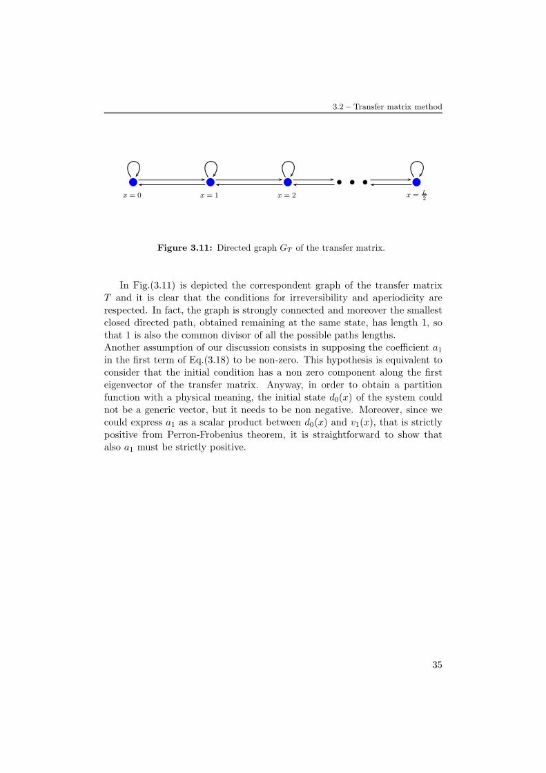
Figure 3.11: Directed graph GT of the transfer matrix.
In Fig.(3.11) is depicted the correspondent graph of the transfer matrixT and it is clear that the conditions for irreversibility and aperiodicity arerespected. In fact, the graph is strongly connected and moreover the smallestclosed directed path, obtained remaining at the same state, has length 1, sothat 1 is also the common divisor of all the possible paths lengths.Another assumption of our discussion consists in supposing the coefficient a1in the first term of Eq.(3.18) to be non-zero. This hypothesis is equivalent toconsider that the initial condition has a non zero component along the firsteigenvector of the transfer matrix. Anyway, in order to obtain a partitionfunction with a physical meaning, the initial state d0(x) of the system couldnot be a generic vector, but it needs to be non negative. Moreover, since wecould express a1 as a scalar product between d0(x) and v1(x), that is strictlypositive from Perron-Frobenius theorem, it is straightforward to show thatalso a1 must be strictly positive.
35


Chapter 4
Triple chain DNA models
The key theme of this work is to study the denaturation process with a ba-sic model of triple chain DNA and verify if an analogue of the Efimov effecttakes place in that system. In fact, the polymeric system that we describedin Chap.2, under scaling hypothesis, is characterized by the presence of aninverse square interaction between chains, very similar to that arising in thequantum case when the Efimov states occur. Indeed, as in the quantum casethe Efimov effect predicts the appearance of three particles bound states atthe two particles resonance point, so we can suppose that an infinite numberof triple chain DNA bound states could appear at the transition point of thetwo chain system.In order to verify this fact, we will build a system analogue to the previouslydescribed two chain system, but with three chains interacting together. Ob-viously such system is more complicated than the previous, both from theanalytical and the computational point of view. In fact, a generic configu-ration of three chains cannot be schematised by a sequence of bubbles androds, as we did in the analytic model for the two chains DNA, because otherdifferent configurations are possible. On the other hand, the great numbersof achievable configurations increase a lot the computation times needed toaddress the problem with the transfer matrix method. Since we are interestedto see the L → ∞ limit, it will be appropriate to take advantage of somesystem symmetries, as we will see in the next section, in order to be able tocompute the eigenvalues of the transfer matrix for a system of dimension L aslarge as possible.Our aim is to verify that variations, predicted in Eq(2.33) for the free energyof the system, that is related to the transfer matrix eigenvalues, effectivelytake place.
37

CHAPTER 4. Triple chain DNA models
x12 x23
Figure 4.1: Three chains paths with periodic boundary conditions.
4.1 Three chains in a cylinder
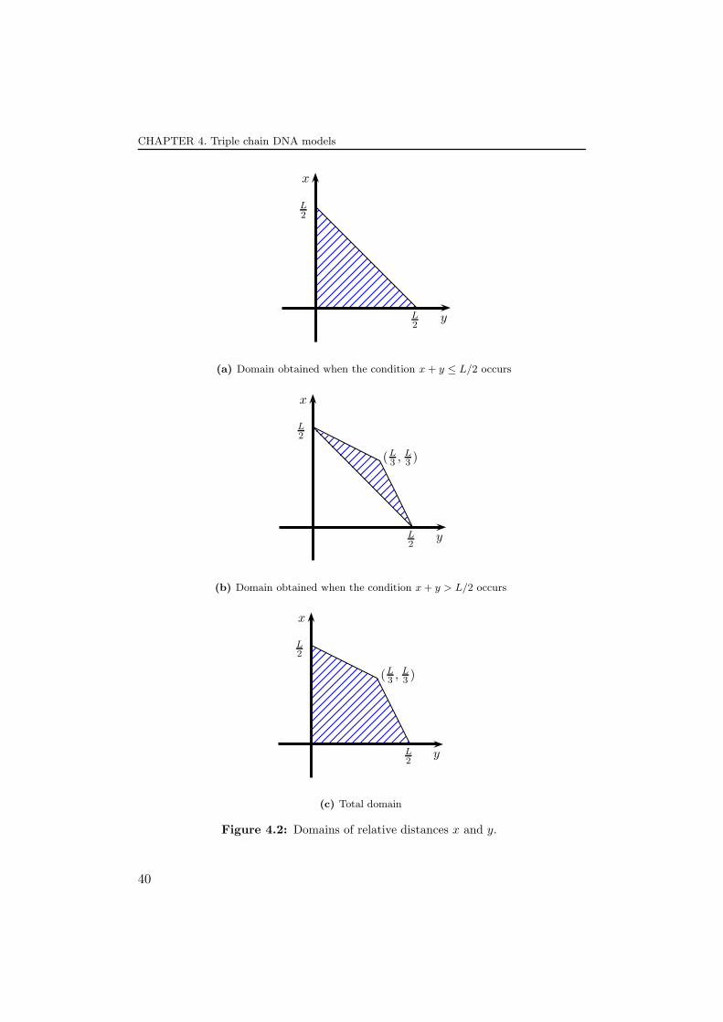
Consider three interacting strands able to move in a cylindrical directed latticewith the rules imposed by the Poland-Scheraga model, described in Sec.(3.1.1),that is banning self intersection and permitting interactions only betweenpoints with the same distance from the origin. (Fig.(4.1)). We associate aweight w when two chains join together and a weight σ when there is a bub-ble opening between two strands, where w and σ are analogue parameters tothose already defined for the two chain model. Instead, when three chainsare involved, or in joint or in breaking a triple-stranded bond, we associaterespectively a weight w2 or σ2ρ, where ρ is a parameter useful to introduce adifferent stacking interaction in the three body case. We set ρ = 1/σ since wechoose chains to interact like two pairs within the triple-stranded arrangement(Fig.(1.3)), based on the chemical nature of the Hoogsteen base pairs.As it is clear from Fig.(4.1), this time there are three possible ending distancesto describe the system states, x12, x23, x13, which are respectively the distancebetween chain 1 and chain 2, between chain 2 and chain 3 and between chain3 and chain 1. Obviously only two of these are independent, so that the par-tition function can depend only from them. Basing ourselves on the naturaldefinition of distance, we choose to utilize the two smallest unsigned distancesof the three. Define indeed x and y the smallest distances and z the largestone. Consider moreover that the largest distance which can be reached in acylinder of base circumference L is L/2. Then we notice that the definitionof z as a function of x and y must change if the condition (x + y) ≤ L/2 or(x+ y) > L/2 occurs.The resulting requests are summarized in Eq.(4.1) and Eq.(4.2).
38

4.1 – Three chains in a cylinder
1. x+ y ≤ L/2
x+ y = z
x ≤ zy ≤ z
=⇒x ≥ 0
y ≥ 0(4.1)
2. x+ y > L/2
x+ y + z = L
x ≤ zy ≤ z
=⇒x ≥ (L− y)/2y ≥ (L− x)/2 (4.2)
In Fig.(4.2) are depicted the domains resulting from Eq.(4.1) end Eq.(4.2),and their union that takes in all the possible configurations for the smallestdistances x and y. From now on we will assume L to be a multiple of six.To write the partition function at fixed distances dN (x, y) we have to con-sider eight different possible moves and their respective weights, as shown inFig.(4.3).
b bb
b
b
b
wδx,0wδy,0
b
b
b
b
b
b
wδx,0wδy,0
b
b
b
b
b
b
σδx,1(w)δy,0
b
b
b
bb
b
σδy,1(w)δx,0
b
b
b
b
b
b
wδx,0wδy,0
b
b
b
b
b
b
wδx,0wδy,0
b
b
b
b
b
b
wδx,0σδy,1
b
b
b
b
b
b
wδy,0σδx,1
Figure 4.3: Possible moves for three strands in an oblique square lattice.
39
CHAPTER 4. Triple chain DNA models
y
x
L2
L2
(a) Domain obtained when the condition x+ y ≤ L/2 occurs
y
x
L2
L2
(L3 ,L3 )
(b) Domain obtained when the condition x+ y > L/2 occurs
y
x
L2
L2
(L3 ,L3 )
(c) Total domain
Figure 4.2: Domains of relative distances x and y.
40

4.1 – Three chains in a cylinder
y
x
L2
L2
(L3 ,L3 )
b b b b b b
b
b
b
b
b
b b b b
b b b b
b b b
b b
b
b
b
b
b
b
b
b
b
Figure 4.4: Possible pairs of distances x and y. The arrows outline the possiblemoves for a chain starting from a particular point, and coloured points are those forwhich not all moves are allowed, so that they need special boundary conditions.
In order to build the recursive equations for dN (x, y) we need to takecare imposing the boundary conditions at the polygon edges in Fig.(4.2c).Obviously our system is discrete because the strands move in a lattice, so thatthe possible couples of distances x and y are given by the points that arelocated into the polygon and separated by the steps shown in Fig.(4.4). Thecoloured points in the picture need a special attention because they cannotallow all permitted moves; in fact they are affected by edges presence. Theblue points are those in which x = z (upper side) or y = z (right lateral side),and starting from them the moves (↑,→,տ) (upper side) and (↑,→,ց)(rightlateral side) are denied, but there are two different ways to take the steps(←, ↓,ց) and (←, ↓,տ). To take this fact into account we have to add a factor2 in the recursive equation for the dN (x, y) every time there is a contributefrom such edges. In order to better figure out this arguments it is useful tosee Fig.(4.5) where a graphic depiction is given.The red points, besides being reached in two ways from each nearby boundarypoint, have also another peculiarity. In fact, starting from this points themoves ↑( under upper side) and → (under right lateral side) are banned, butthere are three ways to remain in the same point instead of two. For example,if we start from the red point with coordinates (L/2−1, 1) to take the step→,
41

CHAPTER 4. Triple chain DNA models
bx
by
(x − 1, y) (x− 1, y + 1) (x, y − 1)
bb
b
b b
b
b b
b
b b
b
b b
b
b b
b
b b
b
Figure 4.5: Possible moves starting from a blue point with x = z. The circleshould depicts the cylindrical lattice seen from above, and the points are the strandsextremities. It is clear that there are two possibilities to take the steps (↓,ց,←)
we see that as the distance y grow of a unity the distance z decrease to L/2−1becoming the smallest together with x, so that the couple of distances whichdefine the partition function dN remains unchanged. To take that into accountwe need to introduce a factor which multiplies by 3 the terms dN−1(x, y − 1)that contribute to dN (x, y − 1) when x and y belong to the upper side, andthe terms dN−1(x− 1, y) that contribute to dN (x− 1, y) when x and y belongthis time to the right lateral side.
The gray points in the left lateral side and in the down side are those inwhich at least one distance x or y is zero. Starting from one of this points it isnot possible to take the steps (←,տ) (lateral side) or (↓,ց) (down side), butthere are two ways to reach the points respective to the moves (→,ց)(lateralside) and (↑,տ) (down side). We need indeed to add in the recursive equationa factor 2 which multiplies every term with a factor σ related to the bubbleopening and a factor 3 which multiplies the terms related to the double bubbleopening. This last is to take account of the point at the origin, because themoves (←, ↓,→,տ) cannot be performed starting from it, whereas (↑,→) canbe performed each three times.In the coloured point that we have listed are included also the polygon verticesas special points, as we will see later.We could further simplify the problem considering the symmetry of the systemunder the exchange of distances x and y. In fact, states identified by thedistances (x, y) or (y, x) results clearly equivalent. Therefore, we could identifyopposite states with respect to the line y = x and reduce the computationof the partition function to those states for which y ≤ x, introducing newboundary conditions (Fig.(4.6)).
42

4.1 – Three chains in a cylinder
y
x
L2
L2
(L3 ,L3 )
b b b b b b
b
b
b
b
b
b
b b b b
b b b b
b b b
b b
b
bb
b
b
b
b
b
b
b
b
b b
b
b
b
bb
b
Figure 4.6: The final domain in the bottom triangle, obtained taking advantage ofthe system simmetry under the exchange of distances x and y.
If we consider only the bottom triangle, starting from the points on the straightline x = y the moves (←,տ, ↑) cannot be allowed, but there are two ways todo the moves (→,ց, ↓). To take that into account we introduce a factor 2 inthe terms coming from this edge which give a contribute in the equation fordN . Moreover, we note that also starting from the new red points under theline y = x there are three ways to remain in the same state.The yellow points have the peculiarity that starting from them there are fourways to remains in the same points, and particularly for those in the bottomside there are two ways that required bubble opening and the other two not.Finally, let’s see the vertices, identified by green dots. Starting from thevertex on top, or from that on the lower left there is only one points that canbe reached in six different ways. While from the vertex on the lower rightthere are two points accessible, the red in four ways and the gray in two.Now we are able to write the recursive equation for the partition function atfixed distances dN (x, y). It is useful to define the following functions
f(y, x) =
3 if (y, x) ∈ red dots
4 if (y, x) = (L/3, L/3 − 1)
2 + 2σ if (y, x) = (1, 0)
2 otherwise
(4.3)
43

CHAPTER 4. Triple chain DNA models
b(yi, xi, y, x) =
2 if (yi, xi) ∈ edge ∧ (y, x) 6∈ same edge
6 if (yi, xi) = (0, 0) | |(yi, xi) = (L/3, L/3)
2 if (yi, xi) = (L/2, 0) ∧ (y, x) = (yi − 1, xi)
4 if (yi, xi) = (L/2, 0) ∧ (y, x) = (yi − 1, xi + 1)
1 otherwise
(4.4)
Then the recursive equation for dN (x, y) can be written as
dN (x, y) = f(y, x)dN−1(x, y)wδx,0wδy,0+
+ dN−1(x− 1, y)σδx,1wδy,0b(y, x− 1, y, x)+
+ dN−1(x, y − 1)(σ)δy,1wδx,0b(y − 1, x, y, x)+
+ dN−1(x− 1, y + 1)wδy,0σδx,1b(y + 1, x− 1, y, x)+
+ dN−1(x+ 1, y)wδx,0wδy,0b(y, x+ 1, y, x)+
+ dN−1(x, y + 1)wδx,0wδy,0b(y + 1, x, y, x)+
+ dN−1(x+ 1, y − 1)wδx,0σδy,1b(y − 1, x+ 1y, x)
(4.5)
where the points (x, y) are contained in the triangle with vertexes in (0, 0),(L/3, L/3) and (L/2, 0).We can now define the transfer matrix for the three chains system, so that
dN (x, y) =∑
(x′,y′)
T[(x,y),(x′,y′)]dN−1(x′, y′)
dN (i) = Ti,jdN−1(j) = TNi,jd0(j)
(4.6)
where we have indexed all the states of the system with a new index i thatruns over every row inside the bottom triangle of Fig.(4.6) in ascending order.An example of the transfer matrix for L = 12 is reported in Eq.(4.8). Wenote that the matrix dimension M is equal to the number of points inside thetriangular domain, and can be obtained by the Pick’ theorem [26], resulting
M = A+ L/2 + 1 = (L2/12) + L/2 + 1 (4.7)
where A is the area of the triangular domain.
44

4.1 – Three chains in a cylinder
T =
2w2 w2
6wσ (2 + 2σ)w w 2ww 2w w 2w w
w 2w w w ww 2w w w w
w 2w 2w w ww 2w w
2σ 2σ 2 12σ 2σ 2 3 1 2
2σ 2σ 1 2 1 2 12σ 2σ 1 2 1 1 1
2σ 4σ 1 3 1 21 1 2 1
1 1 2 3 1 21 1 1 2 2 2 1
1 1 2 11 1 2 1
1 2 2 4 61 2
(4.8)
Since we are in interested in studying the analogy between the Efimovquantum effect and the behaviour of tsDNA bound states, we need to underlinethe analogy between the Eq.(4.6) and an equation of time evolution in thequantum problem
|ψ(t)〉 = e−iHt/h |ψ(0)〉 (4.9)
Such formal analogy, obtained by the identification of the monomer indexwith the imaginary time, suggests us to expect a common behaviour of thehamiltonian eigenvalues and the logarithm of the eigenvalues of the transfermatrix. Obviously this analogy could be affected by the fact that Eq.(4.9)holds for a continuous time and the other one is defined on a discrete lattice.
45


Chapter 5
Results and discussion
In this chapter we report the results we have been able to obtain by increasingthe system dimension as much as possible. In order to optimize the numer-ical computing we took advantage of sparse matrices computation modulesunder Matlab platform (R2013a), and particularly of the eigs function, usefulto compute the largest eigenvalues of the matrix [17]. In this way we havereached a limit system dimension of L = 2940 that corresponds to a transfermatrix dimension of 721.771.In Fig.(5.1) it is shown an illustrative graph for the free energy density withvarying w. The different curves correspond to different small values of L,just to highlight the behaviour of the system near to the transition point.This picture is enough to figure that in the limit L → ∞ the curve beforethe phase transition (w < wt) tends to become constant with limit value− ln 8 = −2, 0794.., similarly to the two chains system with − ln 4. This resultit is also justifiable with entropic arguments, in fact now we have eight possiblemoves for the strands in the lattice, instead of four. Thus we expect to find, innatural units and in the limit L→∞, f = − ln 8 for w = σ = 1 and thereforefor the whole stretch (w < wt) before the phase transition, in the denaturedphase.In the spirit of Efimov effect we expect to find, at the point of the two chaintransition w = 4/3, bound states for the triple chains DNA, resulting in a re-duction of the free energy. This would correspond to find the largest eigenvalueof the transfer matrix bigger than eight, in the limit L → ∞. In Fig.(5.2) isplotted the variation of the free energy density with respect to the denaturedphase (∆f = − ln(λ1/8)) against 1/L. Since we observe it to converge to anegative value, Fig.(5.2) is in agreement with our prediction of the analogywith the Efimov effect.
As in the case of double chains we plot in Fig.(5.3) the relaxation timeξ‖, rescaled to the squared system size, against w for different value of L, to
47

CHAPTER 5. Results and discussion
1.3 1.32 1.34−2.084
−2.08
−2.076
w
f
L = 48L = 72L = 144L = 240
Figure 5.1: Free energy density, σ = 1/2, for varying w.
0.4 0.6 0.8 1 1.2 1.4
x 10−3
−1.178
−1.174
−1.17
−1.166
−1.162
−1.16x 10
−5
1/L
∆f
Figure 5.2: Variation of the free energy density against L, at fixed σ = 1/2, w = 4/3;the last value is achieved for L = 2940.
48

5.1 – Extrapolation
1.3 1.32 1.34 1.36 1.380
0.04
0.08
0.12
0.16
w
ξ ‖/L
2
L = 48L = 72L = 144L = 240
Figure 5.3: ξ‖ rescaled to L2, σ = 1/2, varying w.
emphasize that we expect ξ‖ to diverge, at the transition point, when L→∞.To estimate wt we fit, with a fourth degree polynomial, a set of ten points
located around the maximum with variable w increments and we look for themaximum ξ‖. In Fig.(5.4) we compare the achieved results with those obtainedfrom the two chain system with the same L; it is clear that the two sets ofdata converge at different values. Particularly the limit value of wt of the dataset for the three chain system is clearly smaller than that of the two chain case(4/3), under the reasonable assumption that the sequence be monotonic. Suchshift in the transition point too gives us an evidence of the presence of at leastonethree stranded DNA bound state when the double stranded transition hasnot yet taken place.The problem of assessing the existence of excited trimer bound states is muchmore difficult and we will address it in the next section.
5.1 Extrapolation
The problem to extrapolate the limit of an sequence of data depending on aparameter L, when the latter tends to infinity, is a difficult one. Any possiblechoice of a particular functional form, for data dependence on L, could biasthe reliability of the final outcome.
49

CHAPTER 5. Results and discussion
0 0.004 0.008 0.012 0.016 0.021.3325
1.3335
1.3345
1.3355
1.3365
1/(L/2)
wt
2 chains
3 chains
wt = 4/3
Figure 5.4: Comparison between the two and the three chains wt estimates.
One possible choice to face this task is to assume a particular functional formfor sequence dependence on L. The particular function opted for will dependson a certain number of free parameters that we need to set in order to in-terpolate the data points computed until a finite value Lmax. As has alreadybeen said, it is useful to observe the sequence as a function of 1/L so that wewill consider as our final estimate of the data sequence limit for L → ∞ thefunction value extrapolated at 1/L = 0.It is clear that such method introduces a systematic error due to the choiceof the function form. Our data can be considered free from error except fromthat introduced by numerical precision, that we estimate to be of the orderof 10−12. Indeed, obtaining the function from a least square interpolation,the statistical error obtained from the fit cannot be interpreted as a standarderror.To put into practice what has just been said, we fit our data with differ-ent functions, obtaining different estimates, and observe how such estimateschange by varying the function form. The variability of final extrapolatedvalues, under changing function, gives us an idea of the systematic error in-troduced by function choice.In Fig.(5.5) are shown the interpolations resulting from the comparison of twoand three stranded system transition point. In the two chain case a linearfit of data returns a value of wt entirely in agreement with the analytical re-
50

5.1 – Extrapolation
0 0.004 0.008 0.012 0.016 0.02
1.3325
1.3335
1.3345
1.3355
1.3365
1/(L/2)
wt
2 chains3 chainsquadratic
cubic4th degree
wt = 4/3
linear
Figure 5.5: Comparison between the two and the three chains wt limit, and resultingfit functions.
sult within the fourth digit (wt = 1.3333). While for the three chain systemwe try to fit data with a quadratic (wt = 1.3326), cubic(wt = 1.3327) andquartic (wt = 1.3328) polynomial function . We can indeed assume a sys-tematic error of about 10−4, and give an estimate of the transition point ofwt3 = 1.3327 ± 0.0001, in agreement with the value reported in literature,wt = 1.3326 ± 0.0001 [20].Having quantitatively checked the presence of a shift of the three chain tran-sition point in relation to that of the two chain case, we are now interestedto understand if this behaviour is a consequence of an Efimov-like effect. Inorder to do that we are going to search in our polymeric system, as mainfeatures of the quantum Efimov effect, the presence of an infinite number ofthree particles bound states which obey a geometrical scaling law (Eq.(2.17)).In the transfer matrix theory at the thermodynamic limit we have seen onlythe largest eigenvalue to be meaningful in the free energy computation, butbased on the formal analogy between Eq.(4.6) and Eq.(4.9) we expect thatalso the logarithm of the transfer matrix eigenvalues, following the first, couldbehave in the classical polymer system in the same way of the correspondentquantum energies. If that were the case, we also expect, recalling Eq.(2.33),that the quantities ∆fi = − ln(λi/8) share the same properties of the hamilto-nian eigenvalues of the quantum problem, so that they are negative and follow
51

CHAPTER 5. Results and discussion
0 0.4 0.8 1.2
x 10−3
−0.5
0
0.5
1.5
2.5
3.5
x 10−6
1/L
−ln(λ
2/8)
− ln(λ2/8)
cubic4th degree
5th degree
6th degree
Figure 5.6: ∆f2 and different interpolating functions, w = 4/3, σ = 1/2, three chainsystem.
the analogue of the quantum mechanics scaling law
∆fi+1
∆fi= c (5.1)
where c is a constant value dependent on system features.The transfer matrix eigenvalues, corresponding to the excited states, resultsmaller than eight even at the largest value of L that we have been able toreach. In order to verify if the quantities ∆fi may turn out to be negativein the L → ∞, we will use the extrapolation method already described. InFig.(5.6) and Fig.(5.7) we plotted respectively ∆f2 and ∆f3 against 1/L, withdifferent choices of function forms for the interpolation. In Tab.(5.1) and inTab.(5.2) are listed the extrapolated values, respectively of ∆f2 and ∆f3, byvarying the polynomial function, and compared with those of the three chainnon interacting case (w = σ = 1) for which we don’t expect Efimov effect,since any chain behaves independently from the other chain. Similar resultsare obtained for the other eigenvalues.
We can note that changing polynomial order the limit values ranges aroundzero, so that we are not able to reach a conclusion about his sign; even if itis interesting to observe that the results obtained for the interacting systemdiffer by four orders of magnitude with respect to that obtained for the non
52
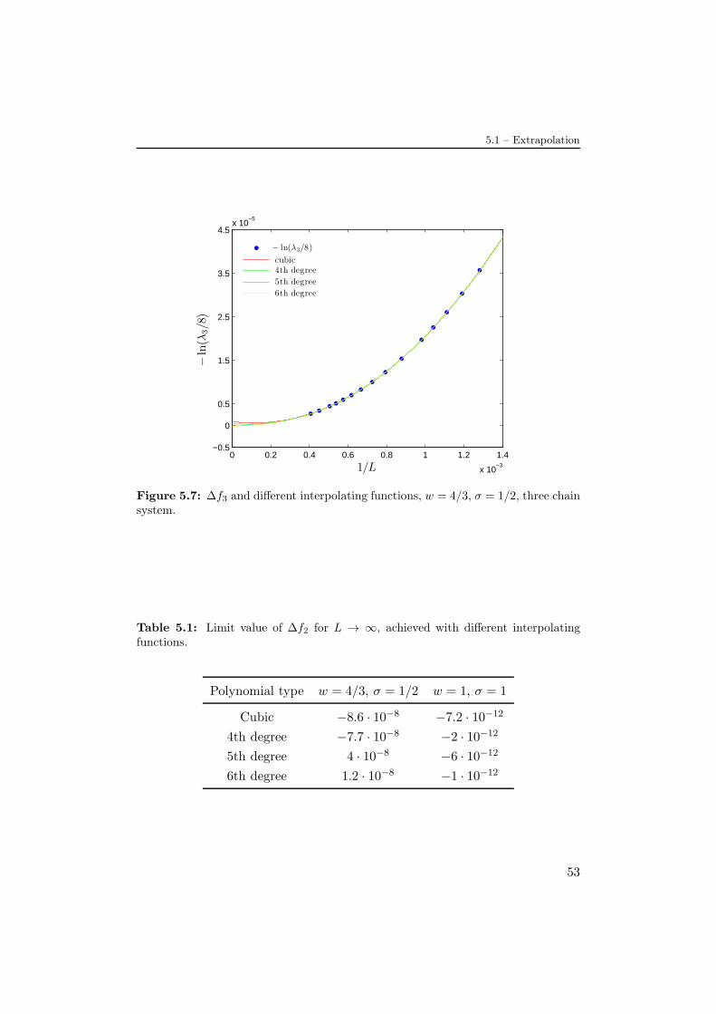
5.1 – Extrapolation
0 0.2 0.4 0.6 0.8 1 1.2 1.4
x 10−3
−0.5
0
0.5
1.5
2.5
3.5
4.5x 10
−5
1/L
−ln(λ
3/8)
− ln(λ3/8)
cubic4th degree
5th degree
6th degree
Figure 5.7: ∆f3 and different interpolating functions, w = 4/3, σ = 1/2, three chainsystem.
Table 5.1: Limit value of ∆f2 for L → ∞, achieved with different interpolatingfunctions.
Polynomial type w = 4/3, σ = 1/2 w = 1, σ = 1
Cubic −8.6 · 10−8 −7.2 · 10−12
4th degree −7.7 · 10−8 −2 · 10−12
5th degree 4 · 10−8 −6 · 10−12
6th degree 1.2 · 10−8 −1 · 10−12
53
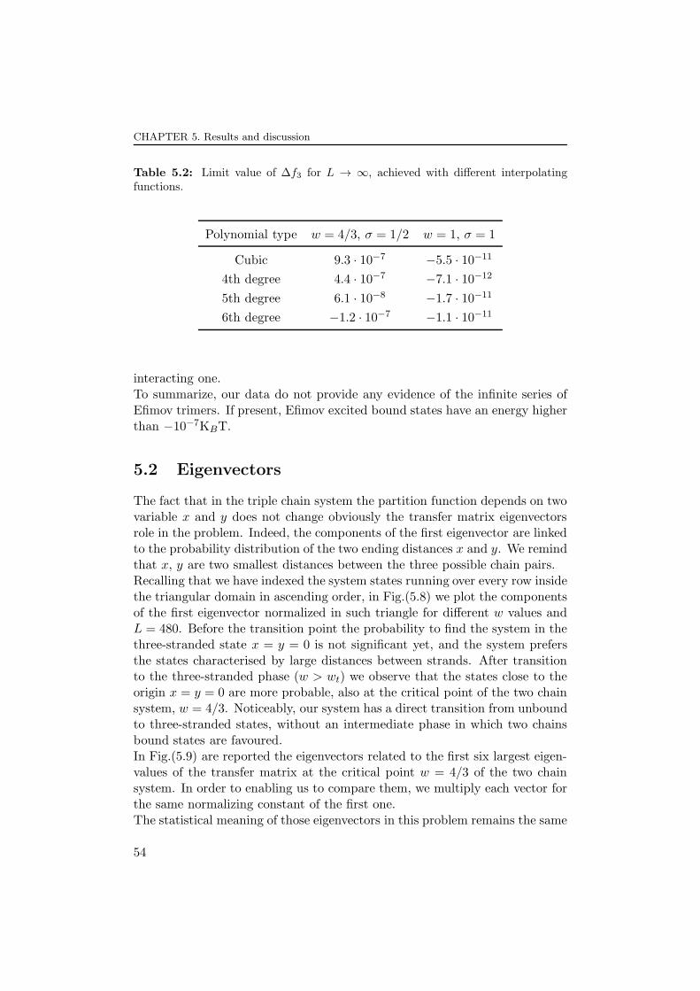
CHAPTER 5. Results and discussion
Table 5.2: Limit value of ∆f3 for L → ∞, achieved with different interpolatingfunctions.
Polynomial type w = 4/3, σ = 1/2 w = 1, σ = 1
Cubic 9.3 · 10−7 −5.5 · 10−11
4th degree 4.4 · 10−7 −7.1 · 10−12
5th degree 6.1 · 10−8 −1.7 · 10−11
6th degree −1.2 · 10−7 −1.1 · 10−11
interacting one.To summarize, our data do not provide any evidence of the infinite series ofEfimov trimers. If present, Efimov excited bound states have an energy higherthan −10−7KBT.
5.2 Eigenvectors
The fact that in the triple chain system the partition function depends on twovariable x and y does not change obviously the transfer matrix eigenvectorsrole in the problem. Indeed, the components of the first eigenvector are linkedto the probability distribution of the two ending distances x and y. We remindthat x, y are two smallest distances between the three possible chain pairs.Recalling that we have indexed the system states running over every row insidethe triangular domain in ascending order, in Fig.(5.8) we plot the componentsof the first eigenvector normalized in such triangle for different w values andL = 480. Before the transition point the probability to find the system in thethree-stranded state x = y = 0 is not significant yet, and the system prefersthe states characterised by large distances between strands. After transitionto the three-stranded phase (w > wt) we observe that the states close to theorigin x = y = 0 are more probable, also at the critical point of the two chainsystem, w = 4/3. Noticeably, our system has a direct transition from unboundto three-stranded states, without an intermediate phase in which two chainsbound states are favoured.In Fig.(5.9) are reported the eigenvectors related to the first six largest eigen-values of the transfer matrix at the critical point w = 4/3 of the two chainsystem. In order to enabling us to compare them, we multiply each vector forthe same normalizing constant of the first one.The statistical meaning of those eigenvectors in this problem remains the same
54

5.2 – Eigenvectors
of previous case, that is their components give us information about the timeemployed by the system to approach the equilibrium state in the thermody-namic limit.
Figure 5.8: Components of the first normalized transfer matrix eigenvector, com-puted at L = 480, σ = 1/2 for different w values. Note the different scales in thecolour bars.
55

CHAPTER 5. Results and discussion
Figure 5.9: Components of the first six transfer matrix eigenvectors, computed atL = 480, σ = 1/2, w = 4/3.
We observe that only for the λ1-eigenvector all components are positive,in agreement with the Perron-Frobenius theorem.The λ1-eigenvector describes a three-stranded bound state, as expected atw > wt. Other eigenvectors describe oscillatory states, that are similar tothose obtained for the non-interacting three-chain (w = σ = 1). This isconsistent with the eigenvalues analysis performed in the previous section.
56

Chapter 6
Conclusions and future
perspectives
In this work we studied the denaturation transition of double-stranded andtriple-stranded DNA-like polymers setting up the transfer matrix techniquewithin simplified 1+1 directed lattice models.We obtained results that give us a new evidence supporting the notion thata shift in the transition point takes place moving from the two chain to thethree chain system. The achieved value of the transition point for the triplestranded DNA is in agreement with that previously reported in literature ofwt = 1.3326 ± 0.0001 [20], to be compared with the exact result wt = 4/3 forthe double-stranded system. w = exp(−ǫ/KBT ) is an adimensional param-eter related to the base-pair interaction energy ǫ. In order to have a finitedenaturation temperature (that is wt > 1), we set σ = 1/2, where σ is theadimensional cooperativity parameter weighting the opening of denaturationbubbles.The transfer matrix method allows us to reach a novel result, estimating thevariation in the free energy, upon addition of the third chain, in correspon-dence of the critical point of the two chain system, that results of the order of−10−5KBT.These results are in line with the prediction by the polymer analogue of thequantum mechanics Efimov effect, that is the presence of three chain boundstates when there is not a correspondent two chain bound state yet.On the other hand, we have not been able to verify the analogy with the otherfeatures present in the Efimov effect, as the appearance of infinite trimer boundstates and the geometrical scaling law for the energy spectrum.The reasons for this could be due to the restrictions imposed by the modelwhich has been used. In fact, the analogue of the quantum effect is predictedin a continuum system, but the transfer matrix method was used to study a
57

CHAPTER 6. Conclusions and future perspectives
model defined on a simplified directed 1+1 lattice.In order to understand the reasons of the incomplete analogy it would beinteresting to study a three-dimensional model for discrete polymer chains.Such choice would enable us to discover if the discrepancies can be due to thediscretization or to the dimensionality of the system. Moreover, the transfermatrix method cannot be used to study a 3-D Poland-Scheraga model andnumerical simulations would be probably the best option, as done for examplein [22].Another interesting perspective would be to further explore the model used inthis thesis by varying the value of the parameter ρ, controlling the coopera-tivity of the three chain bubble opening in the system. Indeed we can foreseethat, by setting it to a small value, a mixed phase of a two chain bound stateand the other one free, takes place in the DNA denaturation process, as al-ready predicted by studying DNA model on a Sierpinsky Gasket [19]. In fact,even though very often the results obtained on the Sierpinsky gasket turn outto be true in the real world, nevertheless it would be interesting to obtain thesame result in a more realistic 1+1 lattice.
58

Bibliography
[1] A.Fonseca and P.E.Shanley. “Efimov effect in an analitically solvablemodel”. In: Nucl.Phys (1979).
[2] A.J.Guttmann and T.Prellberg. “Staircase polygons, elliptic integrals,Heun functions, and lattice Green functions”. In: Phys. Rev. 47 (1993).
[3] Somendra M Bhattacharjee. “Unzipping DNAs: towards the first stepof replication”. In: Journal of Physics A: Mathematical and General 33(2000).
[4] D.Poland and A.Scheraga. “Phase transitions in one dimension and thehelix-coil transition in polyamino acids”. In: J. Chem. Phys 45 (1996).
[5] Maria Duca et al. “The triple helix: 50 years later, the outcome”. In:Nucleic Acids Research (2008).
[6] Andrew M. Essin and David J. Griffiths. “Quantum mechanics of the1/x2 potential”. In: American Journal of Physics (2005).
[7] Keith R. Fox and Tom Brown. “Formation of stable DNA triplexes”. In:Biochemical Society Transactions (2011), 629–634.
[8] Georg Frobenius. “Ueber Matrizen aus nicht negativen Elementen”. In:Sitzungsber. Konigl. Preuss. Akad. Wiss. (1912), pp. 456–477.
[9] Felsenfeld G, Davies DR, and Rich A. “Formation of a three-strandedpolynucleotide molecule”. In: J. Am. Chem. Soc (1957).
[10] K. Hoogsteen. “The crystal and molecular structure of a hydrogen-bonded complex between 1-methylthymine and 9-methyladenine”. In:Acta Crystallographica 16.9 (1963), pp. 907–916.
[11] Watson JD and Crick FH. “Molecular structure of nucleic acids; a struc-ture for deoxyribose nucleic acid”. In: Nature (1953), 737–738.
[12] J.M.Blatt and V.F.Weisskopf. Theoretical Nuclear Physics. 1952.
[13] Rajat K.Bhaduri. “An elementary exposition of the Efimov effect”. In:American Journal of Physics (2011).
59

BIBLIOGRAPHY
[14] Gerasim K.Iliev. “Phase transitions in polymeric systems: a directedwalk study”. In: PhD thesis, University of Toronto (2008).
[15] Bruce Kitchens. Symbolic dynamics: one-sided, two-sided and countable
state markov shifts. Ed. by Springer. 1998.
[16] T. Kraemer et al. “Evidence for Efimov quantum states in an ultracoldgas of caesium atoms”. In: Nature (2006).
[17] R.B. Lehoucq and D.C. Sorensen. “Deflation Techniques for an Implic-itly Re-Started Arnoldi Iteration”. In: SIAM J. Matrix Analysis and
Applications (1996), 789–821.
[18] Mandelkern M et al. “The dimensions of DNA in solution”. In: J Mol
Biol (1981).
[19] Jaya Maji et al. “Melting behavior and different bound states in three-stranded DNA models”. In: Physical review 89 (2014).
[20] Jaya Maji et al. “When a DNA triple helix melts: an analogue of theEfimov state”. In: New Journal of Physics (2010).
[21] M. Mandel and J. Marmur. “Use of Ultraviolet Absorbance-TemperatureProfile for Determining the Guanine plus Cytosine Content of DNA”.In: Methods in Enzymology (1968), pp. 198–206.
[22] D. Marenduzzo et al. “Different pulling modes in DNA overstretching:A theoretical analysis”. In: Physical review 81 (2010).
[23] Mirkin et al. “DNA H form requires a homopurine-homopyrimidine mir-ror repeat”. In: Nature (1987).
[24] M.Masetto. “Denaturazione termica del DNA a tre eliche:un approcciomeccanico statistico”. In: Bachelor’s degree thesis, University of Padua
(2011).
[25] Rajeswari MR. “DNA triplex structures in neurodegenerative disorder,Friedreich’s ataxia”. In: journal of biosciences (2012), pp. 519–32.
[26] Georg Pick. “Geometrisches zur Zahlenlehre”. In: Sitzungsberichte des
deutschen naturwissenschaftlich-medicinischen Vereines fur Bohmen ”Lo-
tos” (1899), 311–319.
[27] S.A.Coon and B.R.Holstein. “Anomalies in quantum mechanics: The1/r2 potential”. In: Am.J.Phys. (2002).
[28] V.Efimov. “Energy levels arising from resonant two-body forces in athree-body system”. In: Physics Letters B 33 (1970), pp. 563–564.
60


![universita' degli studi di padova - [email protected] - Universit](https://static.fdocuments.in/doc/165x107/620619ec8c2f7b1730049ab8/universita-degli-studi-di-padova-emailprotected-universit.jpg)