Universit a degli Studi di Padova - MathUniPDdronzani/docs/md_thesis_ronzani.pdf · Universit a...
104
Universit` a degli Studi di Padova Dipartimento di Matematica Corso di Laurea Magistrale in Informatica Analysis and Comparison of Position-based Routing Protocols for 3D MANETs Relatore Prof. Claudio Enrico Palazzi Laureando Daniele Ronzani Anno Accademico 2014-2015
Transcript of Universit a degli Studi di Padova - MathUniPDdronzani/docs/md_thesis_ronzani.pdf · Universit a...

Universita degli Studi di Padova
Dipartimento di Matematica
Corso di Laurea Magistrale in Informatica
Analysis and Comparison of Position-based
Routing Protocols for 3D MANETs
Relatore
Prof. Claudio Enrico Palazzi
Laureando
Daniele Ronzani
Anno Accademico 2014-2015

Vorrei ringraziare il Prof. Claudio Palazzi, relatore della mia tesi, ed Armir Bujari,
per l’aiuto e il sostegno fornitomi durante la stesura di questa tesi.
Ringrazio la mia famiglia per il sostegno economico e morale, e per essermi stata vicina,
a suo modo, durante tutti i miei anni di studio.
Ringrazio la mia fidanzata per avermi sostenuto, ascoltato e capito in tutto e per tutto,
nonostante le molte difficolta che abbiamo dovuto affrontare insieme. E ringrazio infine
i miei amici e colleghi di universita, per i quali avro un ricordo dei molti piacevoli
momenti vissuti insieme.
Padova, Sep 2015 Daniele Ronzani
iii

Abstract
Recent evolutions of Mobile Ad-hoc Networks (MANETs) have considered microaerial
vehicles (drones), generalizing the topology from a 2D model to a 3D one, thus
generating a 3D MANET or Drone Ad-hoc Network (DANET). Indeed, the capability
of drones to fly generates a scenario where nodes are not just distributed on a plain
surface. This is a very interesting and technically challenging scenario, when considering
routing of messages between endpoints.
The wireless nature of the connection, node mobility and the lack of a communication
infrastructure further complicates the problem of routing messages between endpoints.
This problem is clearly exacerbated in a 3D scenario; yet, the presence of alternative
routes that pass through non-planar multi-hop routes provides new possibilities that
are not well exploited by current state-of-the-art algorithms. It is hence very interesting
for the scientific community to study how routing protocols, designed for 2D scenarios,
have been adapted to deal with 3D MANETs and whether there is a winner approach
among existing ones.
In this context, this thesis focuses on the difficulties and the state-of-the-art of proto-
cols on 3D routing, drawing analysis strengths and weaknesses of all the related routing
protocols proposed so far (to the best of our knowledge). Moreover, a comparison of
these protocols through a common scenario is performed.
v


Table of Contents
1 Introduction 1
2 Background 5
2.1 Mobile Ad-Hoc Networks . . . . . . . . . . . . . . . . . . . . . . . . . 5
2.1.1 Applications of MANET . . . . . . . . . . . . . . . . . . . . . . 6
2.1.2 Drone Ad-Hoc Networks . . . . . . . . . . . . . . . . . . . . . . 7
2.2 The problem of routing in MANETs . . . . . . . . . . . . . . . . . . . 8
2.3 Classification of Routing Protocols . . . . . . . . . . . . . . . . . . . . 9
2.3.1 Topology-based protocols . . . . . . . . . . . . . . . . . . . . . 9
2.3.2 Position-based protocols . . . . . . . . . . . . . . . . . . . . . . 12
3 Routing in 3D Networks 19
3.1 Notation and Preliminaries . . . . . . . . . . . . . . . . . . . . . . . . 19
3.1.1 General Model . . . . . . . . . . . . . . . . . . . . . . . . . . . 19
3.1.2 Terminology . . . . . . . . . . . . . . . . . . . . . . . . . . . . 20
3.1.3 Metrics . . . . . . . . . . . . . . . . . . . . . . . . . . . . . . . 21
3.2 Neighborhood Discovery . . . . . . . . . . . . . . . . . . . . . . . . . . 22
3.2.1 Beaconing . . . . . . . . . . . . . . . . . . . . . . . . . . . . . . 22
3.2.2 Location Request Message . . . . . . . . . . . . . . . . . . . . . 24
3.3 Single-path Forwarding Algorithms . . . . . . . . . . . . . . . . . . . . 25
3.3.1 Deterministic Progress-based Algorithms . . . . . . . . . . . . 25
3.3.2 Randomized Progress-based Algorithms . . . . . . . . . . . . . 35
3.3.3 Face-based algorithms . . . . . . . . . . . . . . . . . . . . . . . 38
3.3.4 3D Hybrid Algorithms . . . . . . . . . . . . . . . . . . . . . . . 49
3.4 Multi-path Forwarding Algorithms . . . . . . . . . . . . . . . . . . . . 52
4 Simulation Environment 55
4.1 Network Simulator 2 (NS-2) . . . . . . . . . . . . . . . . . . . . . . . . 55
4.1.1 Why use NS-2? . . . . . . . . . . . . . . . . . . . . . . . . . . . 56
4.1.2 Basic architecture . . . . . . . . . . . . . . . . . . . . . . . . . 56
4.2 Experimental Scenario . . . . . . . . . . . . . . . . . . . . . . . . . . . 57
4.2.1 Single Flow . . . . . . . . . . . . . . . . . . . . . . . . . . . . . 60
vii

viii TABLE OF CONTENTS
4.2.2 Multiple Flow . . . . . . . . . . . . . . . . . . . . . . . . . . . . 61
5 Performance Evaluation 63
5.1 Comparison of different parameters in randomized-based algorithms . 63
5.2 Standard comparison results . . . . . . . . . . . . . . . . . . . . . . . . 64
5.3 Comparison results with dynamic threshold values . . . . . . . . . . . 71
5.3.1 Dynamic TTLR threshold . . . . . . . . . . . . . . . . . . . . . 71
5.3.2 Dynamic TTLF threshold . . . . . . . . . . . . . . . . . . . . . 71
5.4 Comparison results with noise traffic . . . . . . . . . . . . . . . . . . . 74
5.5 Comparison results with dynamic min path length . . . . . . . . . . . 74
5.6 Summarized Results . . . . . . . . . . . . . . . . . . . . . . . . . . . . 82
6 Conclusions and Future Works 85
References 89

List of Figures
2.1 LAR protocol used with AODV or DSR protocols, to route a packet
from S to D. Node S sends request packets to all neighbors’ nodes inside
the square box (called REQUEST ZONE), limiting flooding forwarding. 13
2.2 Taxonomy of routing algorithms . . . . . . . . . . . . . . . . . . . . . 16
2.3 Performance comparison of DSR and Grid routing protocols. Pictures
taken from [19] . . . . . . . . . . . . . . . . . . . . . . . . . . . . . . . 18
3.1 Two graphs of nodes that represent two wireless networks. Lines are
wireless links that connect each pair of nodes. Figure (a) is a 2D network,
figure (b) is a 3D network. . . . . . . . . . . . . . . . . . . . . . . . . . 20
3.2 Every node has a disk around itself, which represents the coverage area
of its transmission range. Every node that is located inside this disk,
can communicate directly to the done to which the disk belongs . . . . 21
3.3 A step of Greedy algorithm, based on distance between neighbor nodes
and destination node. . . . . . . . . . . . . . . . . . . . . . . . . . . . 27
3.4 A step of Compass strategy, based on angle formed by current node,
neighbor nodes and destination node. . . . . . . . . . . . . . . . . . . . 29
3.5 A loop with Compass. . . . . . . . . . . . . . . . . . . . . . . . . . . . 29
3.6 A step of Most Forward strategy, based on projected distance between
neighbor nodes and destination node. . . . . . . . . . . . . . . . . . . . 30
3.7 A step of Ellipsoid strategy, based on sum of distance between each
neighbor node and destination node and distance between the same
neighbor node and current node. . . . . . . . . . . . . . . . . . . . . . 31
3.8 A local minima example executing Greedy and GEDIR algorithms . . 32
3.9 Path performed by DFS. The node sequence is s− 2− 3− 1− 2− 1−s− 1− 3− 2− 1− 2− s− 1− s− 4− 5− d. . . . . . . . . . . . . . . 33
3.10 In AB3D, plane PL1 passes through s, d and n1, plane PL2 is orthogonal
to PL1. Both planes contain the line sd. . . . . . . . . . . . . . . . . . 37
3.11 Planarization of a graph (a) to extract the GG sub-graph (b). . . . . . 41
3.12 Forwarding steps of Face2 algorithm. . . . . . . . . . . . . . . . . . . . 42
3.13 Nodes projected on a plane . . . . . . . . . . . . . . . . . . . . . . . . 43
ix

x LIST OF FIGURES
3.14 Cross link in red circle . . . . . . . . . . . . . . . . . . . . . . . . . . . 43
3.15 Computing of a plane with Projective face algorithm . . . . . . . . . . 44
3.16 Projection of graph nodes (a) on the three planes xy (b), xz (c) and yz
(d) in CFace(3) algorithm. . . . . . . . . . . . . . . . . . . . . . . . . . 45
3.17 2D graphic representation of computing Least-Squares Projection (LSP)
plane, as the first projection plane. . . . . . . . . . . . . . . . . . . . . 48
3.18 Example of GFG algorithm. Green arrows represents packet forwarding
in greedy-mode, blue arrows are represents packet forwarding in face-mode. 50
3.19 Performing of LAR algorithm. Packets are forwarded only to nodes that
are located within the defined area. . . . . . . . . . . . . . . . . . . . . 53
4.1 Two language structure of NS-2. Class hierarchies in both the languages
(C++ and OTcl) may be standalone or linked together. OTcl class
hierarchy is the interpreted hierarchy and C++ class hiearchy is the
compiled hierarchy . . . . . . . . . . . . . . . . . . . . . . . . . . . . . 56
4.2 Basic architecture of NS-2 . . . . . . . . . . . . . . . . . . . . . . . . . 57
4.3 Node degrees in 10,000 generated graphs with n = 50, 100, 150 and 200 59
5.1 Performance of best parameters combinations in Random Walk, con-
sidering the simulation scenario described in 4.1 with 150 nodes. m is
the number of candidate nodes, R indicates which strategy is used to
choose candidate nodes (random, greedy, compass, most forward), S
indicates how the chances of choosing the next node are made (uniform,
distance, angle, projected distance) and ab indicates if consider planes
subdivision or not. . . . . . . . . . . . . . . . . . . . . . . . . . . . . . 64
5.2 Delivery rate (a), path dilation (b), and delivery time (c) of all algorithms,
in a graph of 50 nodes, with TTLF = 2N (100), TTLR = N (50) and
TTL = 6N (300) . . . . . . . . . . . . . . . . . . . . . . . . . . . . . . 67
5.3 Delivery rate (a), path dilation (b) and delivery time (c) of all algorithms,
in a graph of 100 nodes, with TTLF = 2N (200), TTLR = N (100) and
TTL = 6N (600) . . . . . . . . . . . . . . . . . . . . . . . . . . . . . . 68
5.4 Delivery rate (a), path dilation (b) and delivery time (c) of all algorithms,
in a graph of 150 nodes, with TTLF = 2N (300), TTLR = N (150) and
TTL = 6N (900) . . . . . . . . . . . . . . . . . . . . . . . . . . . . . . 69
5.5 Delivery rate (a), path dilation (b) and delivery time (c) of all algorithms,
in a graph of 200 nodes, with TTLF = 2N (400), TTLR = N (200) and
TTL = 6N (1200) . . . . . . . . . . . . . . . . . . . . . . . . . . . . . . 70
5.6 Delivery rate (a) and path dilation (b) of Random Walk and Greedy-
Random-Greedy algorithms, in a graph of 150 nodes, with TTLR = 75,
150, 225, 300, and a global threshold TTL of 2 ∗ TTLR. . . . . . . . . 72
5.7 Delivery rate (a) and path dilation (b) of Projected Face, CFace(3),
ALSP Face and GFG algorithms, in a graph of 150 nodes, with TTLF
= 150, 300, 450, 600, a global threshold TTL of 3 ∗ TTLF and an ABS
value of 100. . . . . . . . . . . . . . . . . . . . . . . . . . . . . . . . . . 73
5.8 Delivery rate (a) and delivery time (b) of all algorithms, in a graph of
150 nodes with 5 concurrent data streams. . . . . . . . . . . . . . . . . 75
5.9 Delivery rate (a) and delivery time (b) of all algorithms, in a graph of
150 nodes with 20 concurrent data streams. . . . . . . . . . . . . . . . 76
5.10 Delivery rate (a) and delivery time (b) of all algorithms, in a graph of
150 nodes with 40 concurrent data streams. . . . . . . . . . . . . . . . 77
5.11 Delivery rate (a), path dilation (b), and delivery time (c) of all algorithms,
in a graph of 150 nodes with minimum path length of each pair source-
destination of 1, 2 or 3 hops. . . . . . . . . . . . . . . . . . . . . . . . 78
5.12 Delivery rate (a), path dilation (b), and delivery time (c) of all algorithms,
in a graph of 150 nodes with minimum path length of each pair source-
destination of 4, 5 or 6 hops. . . . . . . . . . . . . . . . . . . . . . . . 79
5.13 Delivery rate (a), path dilation (b), and delivery time (c) of all algorithms,
in a graph of 150 nodes with minimum path length of each pair source-
destination of 7, 8 or 9 hops. . . . . . . . . . . . . . . . . . . . . . . . 80
5.14 Delivery rate (a), path dilation (b), and delivery time (c) of all algorithms,
in a graph of 150 nodes with minimum path length of each pair source-
destination greater than 10 hops. . . . . . . . . . . . . . . . . . . . . . 81
List of Tables
3.1 List of randomized algorithm and their attribute values in RW. . . . . 40
4.1 Settings of simulated topology in Single Flow experiment. . . . . . . . 61
4.2 Settings of simulated topology in Multi Flow experiment. . . . . . . . 62
5.1 All the algorithms considered in this thesis, with their characteristic
and performance results. . . . . . . . . . . . . . . . . . . . . . . . . . . 83
xi

xii LIST OF ALGORITHMS
List of Algorithms
1 One step of GEDIR algorithm . . . . . . . . . . . . . . . . . . . . . . . 26
2 One step of Greedy algorithm . . . . . . . . . . . . . . . . . . . . . . . 27
3 One step of Compass algorithm . . . . . . . . . . . . . . . . . . . . . . 28
4 One step of Most Forward algorithm . . . . . . . . . . . . . . . . . . . 30
5 One step of Ellipsoid algorithm . . . . . . . . . . . . . . . . . . . . . . 30
6 One step of DFS algorithm . . . . . . . . . . . . . . . . . . . . . . . . 34
7 One step of Random Walk algorithm . . . . . . . . . . . . . . . . . . . 39
8 Face2 algorithm . . . . . . . . . . . . . . . . . . . . . . . . . . . . . . 41
9 CFace(3) algorithm . . . . . . . . . . . . . . . . . . . . . . . . . . . . . 46
10 Adaptive Least-Squares Projective Face algorithm, refering to [14] adapted
to this thesis. . . . . . . . . . . . . . . . . . . . . . . . . . . . . . . . . 48
11 Greedy-Face-Greedy algorithm . . . . . . . . . . . . . . . . . . . . . . . 51

Chapter 1
Introduction
Mobile ad-hoc networks (MANETs) are networks in which mobile and autonomous
terminals - in this context simply referred to as “nodes” - are connected by wireless
links, even through multi-hop communications, capable of operating without a fixed
infrastructure or centralized administration. Their high flexibility have made MANETs
applicable to a wide set of scenarios including all those cases where a fixed infrastructure
is not available or effective (e.g., rescue teams, operations in remote rural areas, disaster
environments, underwater networking). An ad-hoc network is capable of operating
autonomously and, generally, it is completely self-organizing and self-configuring.
Devices that represent wireless hosts may be notebook computers, PDAs, cell phones,
drones, vehicles, etc, with different memory capacity, energy capacity and computing
power. The main feature of this type of networks is the frequent change of topology,
caused by the uncontrolled motion of the terminals. This makes routing discovery and
maintenance a very challenging task.
Recent evolutions of these networks have considered vehicles (VANETs - Vehicular
ad-hoc networks) and microaerial vehicles (drones or UAVs). While the former changes
the scenario by just adding an increase speed of nodes and a schematic movement
through streets, the latter generalizes the topology from a 2D topology to a 3D one with
a free movement scheme. This difference generates the 3D MANETs or Drone Ad-hoc
Networks (DANETs). Indeed, the capability of drones to fly generates a scenario
where nodes are not just distributed on a plain surface. This is a very interesting and
technically a challenging scenario, especially when considering the routing process. On
the other hand, since the current commercial popularity of drones, this is the first time
we can envision a real practical employment for such 3D MANETs. Therefore, even if
very little scientific literature has been devoted so far to the issues and solutions related
this kind of networks, this is a trend that is going to change very soon, attracting
researchers and practitioners for many years, as well as to become increasingly present
in real applications.
1

2 CHAPTER 1. INTRODUCTION
In a MANET, the communication between two nodes occurs if and only if the
distance between them is less than the minimum between the two nodes’ transmission
ranges. If two nodes are not directly connected, multi-hop forwarding involving
intermediates nodes can be used, running a routing process. The wireless nature of the
connection, the mobility of the nodes and the lack of a communication infrastructure,
make the problem of routing very complex. Mobile hosts are free to move in the space,
resulting in a dynamic network with potentially rapid topological changes and without
notice not known a priori. Hence, routing information is volatile and changes in time.
Moreover, the mobile hosts often use batteries which have a limited energy supply
and the continuous exchange of control messages for network updates may cause a
fast discharge of energy power. These issues are clearly exacerbated in a 3D scenario.
Several routing protocols for ad-hoc networks have been proposed in the recent years
[1, 2].
A typical categorization divides routing protocols into topology-based protocols
and position-based protocols (or geographic-based protocols) [25, 34]. Position-based
routing protocols use a different mechanism for path discovery, which does not need to
maintain routes to destinations. These routing protocols use the geographic position
information of the nodes to perform packet forwarding. The position-based approach in
routing becomes practical due to the recent availability of small, inexpensive low-power
Global Position System (GPS) receivers, and the rapidly developing software and
hardware solutions for determining absolute or relative position of nodes in ad-hoc
networks. Each node determines its own geographic position using a location system,
such as GPS. Therefore, the routing decision at each node can be based only on the
position of node itself, the destination’s position (being either a physical node or
geographical position where data needs to reside), and the neighbors’ position. This
translates into a purely local routing protocols, in which the nodes do not have to
know the status of the entire network and ever have to store routing tables nor do they
need to transmit control messages to keep routing tables.
A scalable routing protocol is one that performs well in a large network. Some
experiments [19, 34] confirm that classic topology-based (AODV, DSDV, or DSR) or
simply flooding-based routing protocols are not scalable. So, when considering large
networks with many nodes, for instance, hundred or thousand of nodes, geographically
based routing protocols, when GPS information is available, would perform better in
terms of achieved data rate, routing table size and low overhead, as demonstrated in
[19]. This is clearly desirable in a 3D MANETs where nodes are drones, which are
nowadays more and more frequently endowed with GPS technology.

3
Contribution
This thesis hence focuses on the analysis and comparison of position-based routing
protocols running in 3D topology networks. After describing the properties and
advantages of the positions-based protocols compared to the topology-based one, a
comprehensive taxonomy of routing protocols for MANETs is proposed, based on the
exploitation of available literature scientific works. Then, with the support of this
taxonomy, a detailed description of all considered position-based protocols is done,
with their possible extensions in 3D networks.
Many routing protocols have been proposed by various researches, using different
models and assumptions. Of course, not all of them are experimented in same simulation
scenario/environment. Therefore, one of the main contribution of this work is to study
these protocols under common assumptions and experimental grounds so as to get an
objective comparison. Performance results, lead to a critical exploration of efficacy
and efficiency. Classical performance metrics have been studied by varying a set of
parameters, providing a comprehensive and extensive analysis of the protocols under
investigation.
The contributions of this thesis are as follows:
(i) Provide a critical analysis, also through common experimental scenario, on the-
state-of-the-art protocols that use geographical position for packet forwarding.
(ii) Provide to the scientific community an implementation of these protocols on a
well known simulator environment, in order to make possible a study support
and future contributions.
(iii) Provide additional insights on the performance of these protocols in real settings.
Organization of thesis
Chapter 2 introduces MANETs, with emphasis of the subclass of DANETs, its
applications and related issues. These concepts are needed to provide some
insights, motivating our work so as to recognize the potential and problems of
this context.
Chapter 3 provides a complete taxonomy of all the routing protocols, with particular
reference to the position-based protocols. The second part of this chapter
describes and analyzes the state-of-the-art of position-based protocols.
Chapter 4 describes the simulator used for tests and the different scenarios generates
for simulations.

4 CHAPTER 1. INTRODUCTION
Chapter 5 shows and analyzes the results obtained from simulations, specifying
the substantial differences that exist between the protocols under dynamic
parameters.
Chapter 6 contains the conclusions and possible future works.
Chapter 2
Background
This chapter gives a background on MANET, including an overview of other subclass
of this type of network, specifying their possible application in real world. Moreover we
discuss the problem of routing in MANETs, with emphasis on position-based routing
protocols and their advantages compared to classical routing protocols. In this context,
a taxonomy of this class of protocols is provided. Finally we discuss the benefits of
using position-based protocols, their potential and how they can improve the routing
compared to topology-based protocols.
2.1 Mobile Ad-Hoc Networks
A MANET consists of a set of mobile nodes that communicate with each other over
wireless links, capable of operating without centralized control or established infras-
tructure. In these settings, nodes can self-organize dynamically and may themselves
act as routers as well. If a node needs to send a packet to another node, the latter
may not be in the transmission range of the first and then intermediate nodes may
be required to collaborate in forwarding the packet from source node to destination
node via multi-hop routing. Since mobile ad-hoc networks may change their topology
frequently, routing in such networks is difficult. There are a number of situations
in which ad-hoc networks are desirable, e.g., in scenarios where infrastructure is not
feasible or cost-effective. They have many potential applications, ranging from environ-
mental monitoring, disaster relief, tactical scenarios etc. Given their popularity and
commercial investment, this technology will continue to have significant attention over
the years to come. In this context, Wireless Sensor Networks (WSNs) are a class of
wireless ad-hoc networks that, characterized by a distributed architecture, are realized
by a set of autonomous electronic devices able to gather data from their immediate
environment and communicate with each other. Wireless networks of sensors are likely
5

6 CHAPTER 2. BACKGROUND
to be widely deployed in the near future because they greatly extend the ability to
monitor and control the physical environment from remote locations, and improve the
accuracy of information obtained via collaboration among sensor nodes and online
information processing at those nodes.
2.1.1 Applications of MANET
Nowadays there are many applications that use MANET technology. Ad-hoc networking
can be applied anywhere where there is little or no communication infrastructure or
the existing infrastructure is expensive or inconvenient to use, e.g., in places where
there are emergency situations such as an earthquake or a tsunami. Ad-hoc networking,
and in particular MANET, allows the devices to maintain connections to the network
as well as easily adding and removing devices to and from the network. The set of
applications for MANET is varied, ranging from large-scale, mobile, highly dynamic
networks, to small, static networks that are constrained by power sources. Typical
applications include:
• Military applications: military equipment contains now some sort of embedded
computer. Ad-hoc networking would allow the military to take advantages of
network technology to maintain an information network between soldiers, vehicles,
airplanes, ships and military information headquarters. The size of military
network is usually very large, because it may have to cover an entire area. This
is a typical scenario in which the use of drones is taking hold.
• Industrial production: industrial applications can require networks for indoor
environment or outdoor environment. Possible applications refer to monitoring
and control of industrial equipment, processes and personnel. Routing in such an
environment can become especially difficult due to obstacles and noise which can
affect the sensor nodes’ line of sight communication, but most of these networks
is static and medium sized, as installed manually in these cases and data can be
routed on pre-determined paths.
• Home applications: these applications refer to indoor environments. Higher
bandwidth might be necessary for gaming or enternainment purposes. The size
of this type of networks is usually little due to the small number of terminals
and needs less energy consumption.
• Health and medical applications: these applications are similar to industrial
applications, but are defined here to be in hospitals and clinics, so inside buildings.
For tracking personnel and patients, a minimum sensor mobility is required. The
size of health network is usually small and uses in-door routing. Among routing
requirements of health applications are reliability, robust routing, high fault
tolerance and high delivery ratio.

2.1. MOBILE AD-HOC NETWORKS 7
• Environmental applications: environmental applications usually refer to
network nodes distributed in certain areas (crops, forests, volcanoes, sea, air,
space). These networks have to be of medium to high size due to the number
of events they may have to detect and track. In physical world surveillance,
sensor networks can be used to track different parameters such as motion, sound,
temperature, light, humidity, atmospheric pressure, etc. In emergency situation
surveillance, nodes may have to track natural catastrophes, detect hazardous
chemical levels, fires, floods etc. WSN is a typical network used for this scenario.
• Automotive applications: a new type of network was considered in the ’80,
based on ad-hoc networks. Networks that involve vehicles are named Vehicular
Ad-hoc Networks. The interest of automotive applications comes from the mobility
of the nodes which are embedded on vehicles and communicate through wireless
technology. The size of such a networks can reach metropolitan areas and this
networks are characterized by nodes that move at different speeds and any
direction.
• Commercial applications: commercial applications refer to small indoor net-
works used in conferences and meetings, or to larger outdoor mesh networks or
extensions to services provided by cellular infrastructure.
Industrial applications, home applications and some health and medical applications
require static routing (or reduced mobility) and small to medium networks. In this
thesis, a focus on techniques that exploit geographic location are done. In a building
of limited geographic area, the use of geographic coordinates doesn’t make sense.
2.1.2 Drone Ad-Hoc Networks
Recently, with the advent of new technologies that make it possible to miniaturize
complex electronic systems, different interesting gadget, that are able to move and fly
autonomously or remotely controlled by a user, were born: these are called drones
or unmanned aircraft vehicles (UAVs). Already many years ago, drone were build,
especially for war environments. Nowadays, given the rapidly growing small unmanned
aircraft industry and their cost reduction, their trade has been extended also in civilian
applications. Thus, drones are also used in a growing number of civil applications,
such as policing and firefighting, and nonmilitary security work, but often preferred
in tactical and battlefield scenarios operated without a human persence, dirty or
dangerous for manned aircraft. Interesting civil applications focuses on search and
rescue missions. Small-scale UAVs can be equipped with imaging sensors for aerial
photography to support rescue people [20]. The use of multiple UAVs rather than
one UAV plays an important role, since the limited flight time of such UAVs and
the fact that search and rescue missions are time critical. Authors in [3] propose the

8 CHAPTER 2. BACKGROUND
problem of deploying a high number of low-cost, low-complexity robots inside a known
environment with the objective that at least one robotic platform reaches each of N
preassigned goal locations. In [23], ab ambitious project is proposed, that tries to
design and build a control system of heterogeneous multi-agents, composed of human,
animals and robots, working in cooperation to solve distributed tasks that require
different technical, physical and cognitive skills. Therefore, this new scenarios require
that those agents could communicate with each other, to exchange relevant information.
These contexts have also introduced the need for a network that extends beyond the
two dimensions, since the altitude is regarded as the third dimension.
2.2 The problem of routing in MANETs
In ad-hoc networks two nodes can communicate with each other (in both directions) if
and only if the distance between them is less than the minimum of their transmission
range. If a node is placed outside the transmission range of a node that wants to
communicate with it, multi-hop routing is used through intermediate communicating
nodes, to send a message from the node to another receiver node. There are various
challenges in MANET such as routing, energy consumption and bandwidth optimization,
but the major challenge is the link failure due to mobility, which causes topology
changes rendering routing information volatile. The utility of routing mechanism makes
it an integral part of any network and there exists a multitude of routing protocols (IP
routing for internet, communication protocols that connect machine, robots, drones,
and protocols for ad hoc networks). Different needs and characteristics of various
networks present specific challenges, requiring appropriate routing techniques.
One way of communication in such networks might seem to simply flood the entire
network. However, the fact that power and bandwidth are scarce resources in such
networks of low powered wireless devices necessitates more efficient routing protocols.
In large networks, with many nodes, the flooding method would cause many collisions
due to contemporary sending of the same packet from multiple nodes and therefore an
increase of the delay time of arrival of the packet to the recipient. Moreover, flooding
causes buffers to fill which translates in packets being dropped when buffers full or
augmented delays due to long packet queuing times. These factors classify this method
as not scalable. A scalable solution is one that performs well in a large network.
Nowadays, there are a number of routing protocols proposed for MANETs to
address the multi-hop routing problem. In general these protocols can be categorized
in topology-based and position-based. Topology-based routing protocols use the
information about the links in the network to perform packet forwarding, position-based
protocols use the position information to make routing decision. Most of position-based
routing protocols are widely used in 2D MANETs, but their performance on 3D
MANETs is not well studied (see 2.3.2.1).

2.3. CLASSIFICATION OF ROUTING PROTOCOLS 9
2.3 Classification of Routing Protocols
Several routing protocols have been proposed to address the routing problem in ad-hoc
mobile environments. Each protocol is based on particular concepts and strategies
which can be advantageous or not based on the type of network on which the protocol
is tailored (network size, number of nodes, range transmission). Mauve et al. [25] and
Stojmenovic [34] divide these protocols in two main categories, topology-based routing
and position-based routing.
2.3.1 Topology-based protocols
Topology-based protocols consider the network topology, and employ routing tables
that specify the best path to route a packet from a source node to a destination node.
These ad-hoc routing systems communicate either topology information or queries
to all nodes in the network. Two important categories that reside in this branch of
protocols are: reactive and proactive. A protocol is said proactive when each node
keeps an up-to-date information reflecting the state of the network and this information
is used when a message should be sent from one node to another to create the route.
A protocol is said reactive when the routing path is created only when necessary.
In the literature, most of the proactive protocols have been proposed in the topology-
based context, in which each node holds information relating to each other node of
the network. The topology-based protocols, in fact, have been primarily designed
for wired networks, or that otherwise have a static structure or that can tolerate
few link disruptions. For this, the protocols based on topology information derive
benefits from this static (if the topology is static, the information on the network
do not change). Proactive protocols can be based on distance-vector strategy (e.g.,
Destination-Sequenced Distance-Vector, DSDV ) and link-state strategy (e.g., Optimized
Link State Routing, OLSR), and constantly discover routes and maintain them in
routing tables. Hello packets are exchanged periodically by which nodes get informed
of changes in the topology.
Instead, when the routes are calculated on a per need basis, reactive protocols
are used. This method presents the main disadvantage of being very slow in forming
the routes, since each node in the creation of the link requires, in on-demand mode,
the connection to subsequent nodes. However, it presents the advantage of incurring
less overhead (due to less control packets flowing in the network), there is less risk
of congestion and the nodes can manage efficiently energy consumption. Ad-Hoc On-
Demand Distance Vector (AODV ) and Dynamic Source Routing (DSR) are examples
of reactive protocols.

10 CHAPTER 2. BACKGROUND
2.3.1.1 Proactive approaches
This section explains some of the state-of-the-art protocols based on proactive mecha-
nism.
Destination Sequenced Distance Vector (DSDV)
Based on the Bellman Ford algorithm, DSDV [9] is a proactive protocol that is
enhanced by the use of sequence numbers in the routing tables (Destination Sequence
Number) to avoid loop problem. In this way, the more updated paths have a higher
sequence number. Each node updates its sequence number every time that it sends
an update. Each node maintains a routing table with an entry for each network node.
Each entry holds a sequence number, which is updated with each change, used to avoid
cycles, and distinguish old routes with the new ones. Each node transmits the updates
periodically or also in case of major changes. When a node receives two paths to the
same node, it chooses the one with greater sequence number, or the one with lesser
hops number in case of equal sequence number. To improve the overhead of network
traffic, this routing protocol uses two type of update packet:
• Full dump: all complete routing information are sent.
• Incremental dump: only updates are sent.
Topology Broadcast on Reverse-Path Forwarding (TBRPF)
TBRPF [30] is another proactive protocol. It transmits only the differences between
the previous network state and the current one. With this routing protocol, each node
computes a spanning tree, formed by all shortest path to all nodes, based on partial
information stored in its topology table. To reduce overhead, each node sends only
part of the spanning tree to its neighbors.
Optimized Link State Routing (OLSR)
Based on link-state algorithm, OLSR [35] is a proactive protocol that tries to reduce
classic flooding and then the overhead. It uses the broadcast of link state information,
to allow each node the reconstruction of the network topology. But this broadcast is
optimized using a system called MultiPoint Relaying (MPR). MPR technique tries
to avoid that each node receives the same message several times, which wastes a lot
of bandwidth. This situation can be improved selecting only some neighbors, called
Multi Point Relays (MPRs). This technique is called partial flooding and perform well
in very dense networks. Link state information is generated only by the MPR nodes.
In OLSR, each node chooses a subset of its neighbors, such that each two-hop away
neighbor is reached through this set. Messages types are:
• HELLO: sent at regular intervals, performs the detection neighbors function,
MPR nodes communication and link sensing.

2.3. CLASSIFICATION OF ROUTING PROTOCOLS 11
• TC (topology control): used to communicate topological information from the
node’s point of view.
• MID: used by the nodes with multiple interfaces to declare its existence to the
rest of the network.
2.3.1.2 Reactive approaches
This section explains some of the state-of-the-art protocols based on reactive mechanism.
Ad-Hoc On-Demand Distance Vector (AODV)
AODV [10] is the reactive version of DSDV. Routes are established on-demand, as
they are needed. An advantage of this approach is that the routing overhead is greatly
reduced, but a disadvantage is a possible large delay from the moment the route
is needed until the time the route is actually acquired. In AODV, the network is
silent until a connection is needed. At that point the network node s that needs
a connection broadcasts a request for connection, sending a Route Request packet
(RREQ) in broadcast on the network, when a path must be found. Other nodes that
receive this RREQ packet, forward it and record the node that they heard it from,
updating the routing information of s, that is, creates or updates the temporary route
to reach the source node in its routing table. This route will serve the Route Reply
packet (RREP) to get to the source. When a node receives such a message and already
has a route to the desired node, it sends a RREP packet though a temporary route
to the requesting node. The needy node then begins using the route that has the
least number of hops through other nodes. Unused entries in the routing tables are
recycled after a time. When a link fails, a routing error is passed back to a transmitting
node sending a Route Error packet (RERR), and the process repeats. Much of the
complexity of the protocol is to lower the number of messages to conserve the capacity
of the network. For example, each request for a route has a sequence number. Nodes
use this sequence number so that they do not repeat route requests that they have
already passed on. Another such feature is that the route requests have a “time to live”
number that limits how many times they can be retransmitted. Another such feature is
that if a route request fails, another route request may not be sent until twice as much
time has passed as the timeout of the previous route request. The advantage of AODV
is that it creates no extra traffic for communication along existing links. Also, distance
vector routing is simple, and doesn’t require much memory or calculation. However
AODV requires more time to establish a connection, and the initial communication to
establish a route is heavier than some other approaches.
Dynamic Source Routing
DSR is similar to AODV, but it uses source routing instead of relying the routing table
at each intermediate node. The source node s sends a RREQ packet, which contains
source address, destination address, request id and path. If a host saw the packet

12 CHAPTER 2. BACKGROUND
before, discards it. Otherwise, the route looks up its route caches to look for a route
to destination. If it is not find, appends its address into the packet and rebroadcast it.
If a node finds a route in its route cache or is the destination, sends a RREP packet,
which is sent to the source by route cache or the route discovery in RREQ packet.
2.3.2 Position-based protocols
Due to changes in topology of mobile environment, the maintenance of routing tables
require an excessive overhead for update network topology information: the network
information must be constantly updated, and this creates an overhead due to the
exchange of control messages. Furthermore, in large networks there are more exchanges
of control messages and routing tables size become very high. For this reason, topology-
based routing protocols become almost useless in more dynamic and large networks.
Position-based (or geographic) routing protocols, use the position of the nodes in the
network to make the forwarding decisions. This position-based approach is introduced
to eliminate some of the limitations of the topology-based protocols in MANETs. These
methods limit the bandwidth required by topology-based routing, because they do not
need to establish and maintains routes, thereby eliminating routing table constructions
and maintenance. The first proposed protocols that use geographic information were
intended to act as a support to the topology-based protocols. For example, one of the
early proposed protocol was Location Aided Routing (LAR), based on DSR, but limits
the propagation of route request packets to a limited geographic region, as seen in Fig.
2.1, where it is most probable for the destination to be located in. In this case, location
information is not used for packet forwarding decision, but it is only used to limit the
propagation area. Over time, many protocols that exploit the position only for the
forwarding decision, have been proposed. This thesis will refer to protocols that use
position information only for the forwarding decision. An overview of position-based
routing protocols and location services can be found e.g. in [25] and [34].
Position-based routing protocols are local, because a node forwards the message
based only on its position, the position of the destination and the position of its
neighbors to which it can communicate directly. Therefore, these protocols do not
require a global knowledge of the network, but they rely on having only a piece of
information (the nodes’ physical location information)1. To use such protocols, it is
necessary for nodes to obtain their coordinates either by using a location service such
as GPS (Global Positioning System) or other types of position services. The position
of a node associates with a neighbor is provided from several mechanism of control
messages (beaconing or request messages). Positional information becomes less current
as that neighbor moves and the accuracy of its position in neighbor table decreases;
1This is not always true. As will be seen later, some protocols use other information to make
decisions, but its complexity is O(1), therefore it is reasonable to also classify these protocols as local.

2.3. CLASSIFICATION OF ROUTING PROTOCOLS 13
RREQS
D
REQUEST ZONE
RREQ
RREQ
r
r
Figure 2.1: LAR protocol used with AODV or DSR protocols, to route a packet from S to
D. Node S sends request packets to all neighbors’ nodes inside the square box
(called REQUEST ZONE), limiting flooding forwarding.
old neighbors may leave and new neighbors may enter radio range. In other words,
neighbor tables can become inconsistent and do not reflect the current state of the
network. For these reasons, the correct choice of beaconing interval to keep nodes’
neighbor tables current depends on the rate of mobility in the network and range of
nodes’ radios. This problem, although not beyond the scope of this thesis, is treated
in chapter 3, section 3.2.
In general, position-based routing protocols have the following characteristics:
• Each node can determine its position (longitude, latitude and altitude) obtained
through a GPS receiver, or another such mechanism.
• Each node can determine the position of its neighbors (usually 1 hop) by using
a location service (for example a set of short request position messages, or a
beaconing system).
• Nodes do not need routing tables to make the forwarding decisions. Each node

14 CHAPTER 2. BACKGROUND
only stores the information about its neighbors (position, speed, direction, etc)
in a neighbor table.
• The routing decision at each hop can be made based on the location of the
current node, its neighbors’ nodes and the destination node.
There are some solutions that require nodes to memorize routes or past traffic,
making these protocols not well scalable. These solutions are sensitive to node queue
size, changes in node activity, and node mobility while routing is ongoing. It is better
to avoid memorizing past traffic at any node if possible. However, the need to memorize
past traffic is not necessarily a demand for significant new resources in the network for
two reason:
• A lot of memory space is available on tiny chips.
• The store of past traffic can be deleted after a certain period of time, when the
routing process is done.
So, the memory usage may be justified in order to improve the performance of some
protocols. An example of routing protocol that use memory is Depth First Search.
2.3.2.1 Routing problem in 3D networks
Position-based routing, unlike topology-based routing, is scalable to a large number
of networks nodes and is efficient when nodes move frequently, because it no need
to keep routing tables up-to-date and no need to maintain a global updated view
of the entire network topology. Establishment and maintenance of routes are not
required, reducing packet overhead, energy and memory capacity considerably. From
this feature, MANET, in particular, derive the best advantage, as these networks are
composed by hosts with limited power energy and limited memory. For 2D networks, a
lot of research has been done about the problem of position-based routing; however, in
real scenarios, nodes may be distributed in 3D space and the extension of 2D routing
protocols into 3D protocols is not trivial. Topology-based routing protocols are not
sensitive to the addition of the third dimension because they rely on a link-state system
knowledge. Instead, position-based protocols are based on the spatial position. In a
three-dimensional space some assumptions made in 2D, such as the ability to extract
planar subgraphs, break down. Durocher et al. [32] shows the impossibility of routing
protocols that guarantee delivery in three-dimensional ad-hoc networks, when nodes
are constrained to have information only about their k-hop neighborhood, in contrast
to the two-dimensional case, where a protocol that uses 1-local algorithm, such as face
routing (see section 3.3.3), guarantees delivery. This leads the problem of finding other
solutions that can guarantee the delivery of packets, with the least use of resources.
Some works have proposed several algorithms that try to achieve a higher delivery

2.3. CLASSIFICATION OF ROUTING PROTOCOLS 15
rate, with a smaller number of node involved. This thesis takes these and compares
them in a fits-all simulation, to obtaining their performance.
2.3.2.2 Taxonomy
Position-based routing protocols can be divided in two main types of packet-forwarding
strategies:
• Single-path forwarding: with single path strategy, an algorithm forwards the
packet in every step to one of its neighbors. Algorithms that uses single path
strategies may be even more robust and with less communication overhead.
• Multi-path forwarding: in this strategy the current node forwards the packet
to all or part of its neighbors. Flooding can be costly in terms of wasted bandwidth,
because packet become duplicated in the network. Moreover, duplicate packets
may circulate forever in loop, unless certain precaution.
Single path forwarding algorithms consider another subdivision based on the type of
geometric or mathematical concepts used for forwarding decision:
• Deterministic progress-based: with deterministic progress based routing
algorithms, the current node (the node holding the packet) forwards the packet
at every step to one of its neighbors that make progress to the destination.
• Randomized progress-based: this strategy is similar to deterministic progress-
based method but in this case the next node is chosen uniformly at random
or according to a probability distribution, from the set of neighbor nodes or
candidate nodes.
• Face-based it is a strategy that allows to arrive at a delivery-rate close to
100% in some cases. In the context of a two-dimensional space, face-based
algorithms allows progress between the faces defined by the nodes considering
the right-hand rule, with which always guarantee reaching the destination. In the
three-dimensional space, the concept of “face” can not be extended, but some
approaches have been proposed that are based mainly on the projection of points
in a plane.
2.3.2.3 Advantages of position-based routing
Position-based routing algorithms are born initially to deal with the requirement
of using less resources. The reasoning behind the position-based algorithms is the
following: if it is possible know the location of the destination and the neighboring

16 CHAPTER 2. BACKGROUND
Figure 2.2: Taxonomy of routing algorithms
nodes, then we can eliminate all the work for the route search and the current node may
send the packet directly to its neighbors which are located “towards” the destination
node.
This section aims to provide an explanation of which are the metrics that provide a
clear gap between the performance of the two routing strategies (positions-based and
topology-based) and then the reasons why the position-based perform well in specific
context. Stojmenovic [34] says that routing protocols that do not use geographic
location in the routing decisions, such as AODV, DSDV, or DSR are not scalable.
Furthermore, because of high mobility of the nodes in MANETs, the route update
may be more frequent than the route requests and some of bandwidth is wasted due to
most of the routing information is never uses. Reactive protocols (e.g., AODV ) reduce
number of broadcasts by establishing routes on demand basis and does not maintain
the whole routing information of all nodes in the network, but need to use flooding to
propagate route request packets (RREQ) in the entire network. If the number of nodes
is very high and the communication requests are very frequent, the flooding mechanism
becomes unsustainable. But on the other hand the use of flooding is necessary to
ensure reaching the destination node. This means that topology-based protocols are
not scalable, due to the effects on broadcast storm problem, while it is likely that only
position-based approaches provide satisfactory performance for large networks.
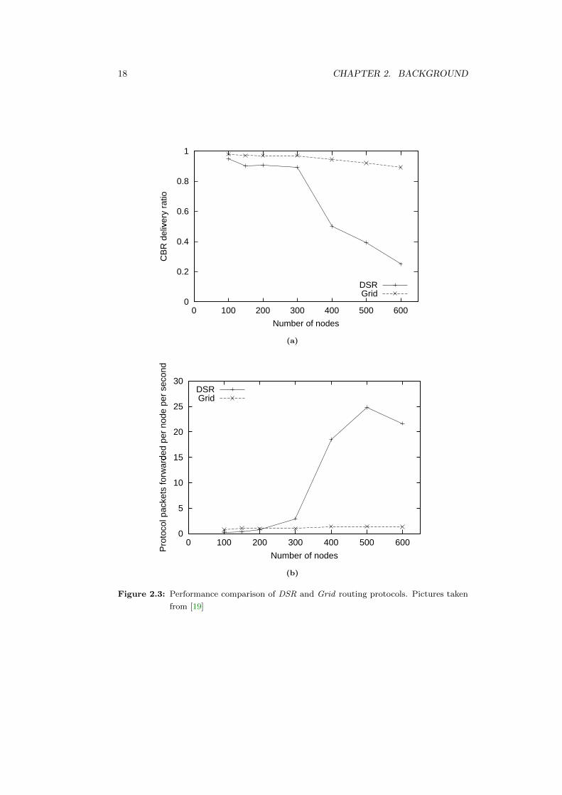
In [19] an experiment compares a geographic forwarding algorithm, called Grid
(similar to Greedy, described in 3.3.1) with DSR protocol. Grid uses GLS (Scalable
Location Service), a distributed location service that tracks mobile node locations.
Experiments, using the ns simulator for up to 600 mobile nodes, show that the

2.3. CLASSIFICATION OF ROUTING PROTOCOLS 17
storage and bandwidth requirements of GLS grow slowly with the size of the network.
Comparing Grid with DSR, in a simulation with nodes that move with a maximum
speed of 10 m/s, [19] obtains two pictures: Fig. 2.3a, that show the fraction data
packets that are successfully delivered in simulations for increasing number of nodes,
and Fig. 2.3b, that shows the number of two protocols packets forwarded per node per
second as a function of the total number of nodes.
In Fig. 2.3a most of the data packets that Grid fails to deliver are due to GLS
query failures; once Grid finds the location of a destination, data losses are unlikely,
since geographic forwarding adapts well to the motion of intermediate nodes. Below
400 nodes, most of the DSR losses are due to broken source routes, but at 400 nodes
and above, losses are mainly due to flooding-induces congestion. So, Grid does a better
job than DSR, especially in large networks. Fig. 2.3b counts only protocol packets
(route request, route reply, hello, etc.). DSR produces less control overhead for small
networks, but at 400 nodes and above, suffers from network congestion and almost
half of the route reply and cache reply messages are dropped due to congestion which
causes new insertions of even more route requests into the network. Also, the source
route is vulnerable to failure. Grid produces less overhead for large networks, because
only local exchange of position information, through small packets, occurs.
18 CHAPTER 2. BACKGROUND
0
0.2
0.4
0.6
0.8
1
0 100 200 300 400 500 600
CB
R d
eliv
ery
ratio
E
Number of nodes
DSRGrid
Figure 14: The fraction of data packets that are successfullydelivered in simulations for increasingnumbers of nodes.Thenodesmove with a maximum speedof 10 m/s.
purposesof comparisonwe includeresultsfor theDSR[10] proto-col. This maynotbea fair comparisonsinceDSRis optimizedforrelatively smallnetworks[3].
Figure14showsthefractionof datapacketssuccessfullydelivered.Most of the datapackets thatGrid fails to deliver aredueto GLSquery failures; thesepackets never leave the source. OnceGridfinds the locationof a destination,datalossesareunlikely, sincegeographicforwardingadaptswell to the motion of intermediatenodes.Below 400nodes,mostof theDSRlossesaredueto brokensourceroutes;at 400 nodesand above, lossesaremainly due toflooding-inducedcongestion.Grid doesabetterjob thanDSRoverthewholerangeof numbersof nodes,especiallyfor largenetworks.
Figure15 shows the messageoverheadof theGrid andDSRpro-tocols. Only protocolpackets are included. In the caseof Grid,theseareHELLO, GLS update,and GLS query and reply pack-ets.In thecaseof DSR,thesearerouterequest,reply, cachedreplypacketsetc. DSR produceslessprotocoloverheadfor small net-works, while Grid produceslessoverheadfor large networks. At400 nodesandabove, DSR suffers from network congestion.Al-mosthalf of theroutereply andcachereply messagesaredroppeddueto congestionwhich causesDSRto inject evenmoreroutere-questsinto the network. Also, as the network grows larger andcongestionbuilds up, the sourcerouteis morevulnerableto fail-ure which will alsoinduceDSR sourcenodesto sendmorerouterequestpackets. DSR’s overheaddropsat 600 nodesbecauseitcould not sendmuchmorepackets in the presenceof congestion.We presentoverheadin termsof packetsratherthanbytesbecausemediumacquisitionoverheaddominatesactualpacket transmissionin 802.11,particularlyfor thesmallpacketsusedby Grid.
7. Future WorkOneareaof the GLS protocol that could be improved is the han-dling of nodemobility. Accuratemovementmodelsmayallow usto integratemovementpredictioninto theGLS protocol. Our cur-rent systemmakes little effort to predict the movementof nodesover long time periodsbecauseour movementmodel is random-ized,but in therealworld anodemaynotneedto updatea locationserver asoftenif its velocity is constantor predictable.
Currently the GLS protocolmakes little effort to proactively cor-
0
5
10
15
20
25
30
0 100 200 300 400 500 600
Pro
toco
l pac
kets
forw
arde
d pe
r no
de p
er s
econ
d
F
Number of nodes
DSRGrid
Figure 15: The number of all protocol packets forwarded pernodeper secondasa function of the total number of nodes.Nodata packets are included. The nodesmove with a maximumspeedof 10 m/s.
rect out-of-dateinformationwhen, for instance,a nodecrossesagrid boundaryline. Proactive updatesmay reducethe incidenceof queryfailures.However, the tradeoff is obvious—caremustbetakennot to consumetoomuchbandwidthwith theupdates.An al-ternatestrategy to addressthesameproblemis to placelesstrustinlocationsobtainedfrom distantlocationservers. Ratherthantrusta distantlocationserver to pinpoint the order-1 squarein which anodeis located,a querycould be moved to, for instance,the sur-roundingorder-3 square.Therethequerycanberestartedwith thefresherinformationavailablein thatsquare
Anotherpotentialareaof improvementis adaptingto nodedensity.If anorder-1 squarebecomestoo crowded,eachnodewill get lessbandwidthfrom thesharedradiospectrum,andeachnodewill haveto work harderto keepits neighbortableup to date. Radioswithvariablepower levels would helpalleviate this problemby chang-ing the effective densityof nodeswithin radio range. In addition,eachsquarein theGLSmaymakealocaldecisionabouthow finelyto sub-divide itself; distantareasneednot agreeon thesizeof theorder-1 square.
Finally, aswe notedearlier, the choiceof a grid basedsystemissomewhatarbitrary. In fact,certainpartitioningschemesoffer thepossibility of betterscaling. The numberof locationservers thata nodemustrecruit is equalto the numberof neighborsper levelin the geographichierarchymultiplied by the numberof levels inthehierarchy. For agrid basedsystem,thismeansthatanodemustmaintainG ��H I�J � serversin anetwork thatis � timesthesizeof thecoverageareaof a singleradio. It is possible,however, to split theworld in half at eachlevel, ratherthanin fourths,by usingrectan-gleswith anaspectratio of �'� � ! . At successive levels,eachsuchrectanglemaybedividedinto two suchrectangles.This leadsto anetwork in which nodesmustrecruitonly ��H I � � locationservers,or ! ��G thenumberof serversneededin a grid basedapproach.
8. ConclusionsWirelesstechnologyhasthepotentialto dramaticallysimplify thedeploymentof datanetworks. For themostpart this potentialhasnot beenfulfilled: mostwirelessnetworksusecostlywired infras-tructurefor all but thefinalhop.Ad hocnetworkscanfulfill thispo-tentialbecausethey areeasyto deploy: they requireno infrastruc-
(a)
0
0.2
0.4
0.6
0.8
1
0 100 200 300 400 500 600
CB
R d
eliv
ery
ratio
E
Number of nodes
DSRGrid
Figure 14: The fraction of data packets that are successfullydelivered in simulations for increasingnumbers of nodes.Thenodesmove with a maximum speedof 10 m/s.
purposesof comparisonwe includeresultsfor theDSR[10] proto-col. This maynotbea fair comparisonsinceDSRis optimizedforrelatively smallnetworks[3].
Figure14showsthefractionof datapacketssuccessfullydelivered.Most of the datapackets thatGrid fails to deliver aredueto GLSquery failures; thesepackets never leave the source. OnceGridfinds the locationof a destination,datalossesareunlikely, sincegeographicforwardingadaptswell to the motion of intermediatenodes.Below 400nodes,mostof theDSRlossesaredueto brokensourceroutes;at 400 nodesand above, lossesaremainly due toflooding-inducedcongestion.Grid doesabetterjob thanDSRoverthewholerangeof numbersof nodes,especiallyfor largenetworks.
Figure15 shows the messageoverheadof theGrid andDSRpro-tocols. Only protocolpackets are included. In the caseof Grid,theseareHELLO, GLS update,and GLS query and reply pack-ets.In thecaseof DSR,thesearerouterequest,reply, cachedreplypacketsetc. DSR produceslessprotocoloverheadfor small net-works, while Grid produceslessoverheadfor large networks. At400 nodesandabove, DSR suffers from network congestion.Al-mosthalf of theroutereply andcachereply messagesaredroppeddueto congestionwhich causesDSRto inject evenmoreroutere-questsinto the network. Also, as the network grows larger andcongestionbuilds up, the sourcerouteis morevulnerableto fail-ure which will alsoinduceDSR sourcenodesto sendmorerouterequestpackets. DSR’s overheaddropsat 600 nodesbecauseitcould not sendmuchmorepackets in the presenceof congestion.We presentoverheadin termsof packetsratherthanbytesbecausemediumacquisitionoverheaddominatesactualpacket transmissionin 802.11,particularlyfor thesmallpacketsusedby Grid.
7. Future WorkOneareaof the GLS protocol that could be improved is the han-dling of nodemobility. Accuratemovementmodelsmayallow usto integratemovementpredictioninto theGLS protocol. Our cur-rent systemmakes little effort to predict the movementof nodesover long time periodsbecauseour movementmodel is random-ized,but in therealworld anodemaynotneedto updatea locationserver asoftenif its velocity is constantor predictable.
Currently the GLS protocolmakes little effort to proactively cor-
0
5
10
15
20
25
30
0 100 200 300 400 500 600
Pro
toco
l pac
kets
forw
arde
d pe
r no
de p
er s
econ
d
F
Number of nodes
DSRGrid
Figure 15: The number of all protocol packets forwarded pernodeper secondasa function of the total number of nodes.Nodata packets are included. The nodesmove with a maximumspeedof 10 m/s.
rect out-of-dateinformationwhen, for instance,a nodecrossesagrid boundaryline. Proactive updatesmay reducethe incidenceof queryfailures.However, the tradeoff is obvious—caremustbetakennot to consumetoomuchbandwidthwith theupdates.An al-ternatestrategy to addressthesameproblemis to placelesstrustinlocationsobtainedfrom distantlocationservers. Ratherthantrusta distantlocationserver to pinpoint the order-1 squarein which anodeis located,a querycould be moved to, for instance,the sur-roundingorder-3 square.Therethequerycanberestartedwith thefresherinformationavailablein thatsquare
Anotherpotentialareaof improvementis adaptingto nodedensity.If anorder-1 squarebecomestoo crowded,eachnodewill get lessbandwidthfrom thesharedradiospectrum,andeachnodewill haveto work harderto keepits neighbortableup to date. Radioswithvariablepower levels would helpalleviate this problemby chang-ing the effective densityof nodeswithin radio range. In addition,eachsquarein theGLSmaymakealocaldecisionabouthow finelyto sub-divide itself; distantareasneednot agreeon thesizeof theorder-1 square.
Finally, aswe notedearlier, the choiceof a grid basedsystemissomewhatarbitrary. In fact,certainpartitioningschemesoffer thepossibility of betterscaling. The numberof locationservers thata nodemustrecruit is equalto the numberof neighborsper levelin the geographichierarchymultiplied by the numberof levels inthehierarchy. For agrid basedsystem,thismeansthatanodemustmaintainG ��H I�J � serversin anetwork thatis � timesthesizeof thecoverageareaof a singleradio. It is possible,however, to split theworld in half at eachlevel, ratherthanin fourths,by usingrectan-gleswith anaspectratio of �'� � ! . At successive levels,eachsuchrectanglemaybedividedinto two suchrectangles.This leadsto anetwork in which nodesmustrecruitonly ��H I � � locationservers,or ! ��G thenumberof serversneededin a grid basedapproach.
8. ConclusionsWirelesstechnologyhasthepotentialto dramaticallysimplify thedeploymentof datanetworks. For themostpart this potentialhasnot beenfulfilled: mostwirelessnetworksusecostlywired infras-tructurefor all but thefinalhop.Ad hocnetworkscanfulfill thispo-tentialbecausethey areeasyto deploy: they requireno infrastruc-
(b)
Figure 2.3: Performance comparison of DSR and Grid routing protocols. Pictures taken
from [19]

Chapter 3
Routing in 3D Networks
This chapter describes the current state-of-the-art of position-based protocols and their
modus-operandi. The overview starts by discussing single-path forwarding strategy
algorithms, introducing the necessary terminology and concepts needed to better
comprehend multi-path approaches. These two strategies perform differently, in terms
of delivery rate and path dilation.
3.1 Notation and Preliminaries
3.1.1 General Model
In the following we will use this conventions and notations:
• A model of MANET is represented, in R2 and R3 spaces, by a geometric graph
G = (V,E), consisting of a finite set V = v1, v2, ..., vN of nodes and a subset
E of cartesian product V × V , the elements called edges (links from a node to
another). Fig. 3.1 shows two model of graphs, that represent two examples of
networks.
• All nodes have the same communication range r, which is represented as a disc
in 2D space and as a sphere in 3D space. The graphs thus obtained is called
Unit Disk Graph, UDG(V, r) and Unit Ball Graph, UBG(V, r) respectively. An
example of Unit Disk Graph is represented in Fig. 3.2
• We define dist(u, v) as the distance between two nodes u and v, given by the
formula of the Euclidean distance:
dist(u, v) =√
(ux − vx)2 + (uy − vy)2 + (uz − vz)2
19

20 CHAPTER 3. ROUTING IN 3D NETWORKS
• Two nodes are said to be neighboring and connected by a link if the Euclidean
distance is at most r:
u is neighboring of v if dist(u, v) ≤ r
• For a node u, we define the set of its neighbors as N(c)
• A path from a node s to a node d is a sequence of nodes s = v1, v2, ..., vk = d,
such that vi and vi+1, 1 ≤ k − 1, are neighbors.
9
35
36
28
2
33
40
49
6
20
4
22
41
4321
18
31
32
48
42
46
44
50
14
5
10
27
17
19
16
3
739
47
37
15
25
13
38
34
12
111
8
45
26
30
23
29
24
(a)
23
30
6
25
11
53
43
15
39
10
58
31
13 38
35
24
42
48
9
5
36
41
44
60
28
40
32
20
29
3
59 33
54
46
49
57
18
27
26
12
56
16
8
34
45
1
37
2
17
50
47
524
5121 22
55
14
19
7
(b)
Figure 3.1: Two graphs of nodes that represent two wireless networks. Lines are wireless
links that connect each pair of nodes. Figure (a) is a 2D network, figure (b) is a
3D network.
3.1.2 Terminology
In order to provide a uniform and fair treatment of all algorithms, a common terminology
to define uniform concepts is introduced.
• The source node is the node that sends the packet, and destination node is the
node that receives the packet. They are called respectively s and d.
• The current node is the node that applies the algorithm at a given time and that
has in its memory the package to be forwarded, and is called c.
• The previous node is the node that sent the packet to c in the previous step, and
is called prev.

3.1. NOTATION AND PRELIMINARIES 21
r
Figure 3.2: Every node has a disk around itself, which represents the coverage area of its
transmission range. Every node that is located inside this disk, can communicate
directly to the done to which the disk belongs
• The neighborhood of the current node c is the set of all nodes connected directly
to c, called N(c). The size of N(c) is indicated with n.
• The disk centered at node c with radius r is called disk(u, r) and covers the
transmission area of c in two-dimensional space.
• The sphere centered at node c with radius r is called ball(u, r) and covers the
transmission area of c in three-dimensional space.
3.1.3 Metrics
In this thesis we are interested in the following performance metrics for routing
protocols.
• Delivery Rate: delivery rate is the ratio of the number of packets received by
the destination (or destinations) to the number of packets sent by the source (or
sources). The first goal that a routing algorithm must achieve is get a guaranteed
delivery rate. Unfortunately many algorithms based on heuristic techniques fail
to reach a delivery rate of 100%.
DeliveryRate% =NumberDataPacketReceived
NumberDataPacketSent∗ 100
• Path Dilation: path dilation is the ratio of the number of hops traversed by
the package during execution of the algorithm to the length of shortest path.
The secondary goal, but not the least important, is to get a path dilation close
as possible to 1, that is, the routing algorithm must travel a path of length as
close as possible to the length of the shortest path.
PathDilation =HopsRoutedByAlgorithm
MinimumPathLength

22 CHAPTER 3. ROUTING IN 3D NETWORKS
• Delivery Time: in this work, the delivery time is defined as the time spent
from when the package arrives from the MAC layer of the source node to the
delivery of the same packet at the recipient node. This metric can be traced
back to the number of hops paths, but, as in this thesis we evaluate real-world
scenarios, we need an index of time. Sometimes, the delivery time is proportional
to the path dilation.
DeliveryT ime = time(PacketDelivered)− time(GetPacketFromMAC)
The above metrics are analyzed by dynamic parameters such as the number of nodes
in the network, the value of threshold, and others, to evaluate the behavior of the
algorithms.
3.2 Neighborhood Discovery
In position-based routing protocols, each node must know the location of all its neigh-
bors. There are several techniques for acquiring this information, based on a periodic
beacon exchange (proactive approach) or location request messages (reactive approach).
This chapter aims to provide an overview of the techniques of the neighborhood dis-
covery. One of these techniques is in fact incorporated in the implemented routing
protocols of this thesis, in order to bring simulations to a more real context, that is
without the ideal situation that the nodes know a priori their neighbors.
With a periodic beacon exchange, beaconing method, each node sends in broadcast
a small packet, called “beacon” that contains its identity, position and other informa-
tion (e.g., its speed and direction). Neighbor nodes receiving this beacon and store
location information in their neighbor-table. This is a proactive approach and is totally
independent of the data traffic. With the location request message the node that holds
a packet and has to forward it, sends in broadcast a request message that contains its
identify. The neighbor nodes that receive the request message from a node, reply with
an hello packet that contains location information and its identify, and send it to the
requester node. This is a reactive approach and depends of the data traffic.
3.2.1 Beaconing
The problem of neighborhood discovery can be identified when the network nodes
move. If a periodic beacon between nodes is started, the speed of nodes can affect the
correctness of position information. Inaccurate or out-dated neighborhood information
may severely affect position-based routing protocols. If a periodic beaconing is used,
there are three different situations that can occur when nodes moves:

3.2. NEIGHBORHOOD DISCOVERY 23
1. Nodes are listed in the neighbor table with an inaccurate position, but are still
accessible.
2. A node moves within the transmission range of another node, but was not visible
before (because it had not received the beacon). So, routing makes a not great
decision, since it does not know that there is a new node maybe as good.
3. A node moves out of transmission range of another node. So, the routing has still
that node in its neighbor table and may send a message to it, but the MAC layer
is unable to reach the node. After some retransmission, the MAC layer drops the
message or notify that it was not able to send and send back the packet. Then,
the routing protocol selects a different next hop and sends back the packet to
the MAC layer. This re-routing has three consequences:
• Delay grows.
• Effective bandwidth decreases.
• Battery discharges.
In addition to the incorrect position information, the beaconing system has other
problems, as the unnecessary use of network resources and the interference with data
traffic. In [24], authors analyze the impact of inaccurate and out-dated neighbor
information on the performance of the network for position-based routing, and propose
some solutions that can solve these problems. They explain that no research has
investigated this problem, which could become important for the effectiveness and
efficiency of position-based routing.
3.2.1.1 Beaconing Strategies
To improve the accuracy of the beaconing, several strategies are proposed:
• Time-based beacon: each node sends a beacon periodically (every t seconds).
• Distance-based beacon: each node sends a beacon only when it is moved of d
meters from its original last sending position.
• Speed-based: the frequency of the beacons is proportional to the speed of the
nodes.
In [24] simulations are carried to see the effectiveness of these beaconing strategies
varying the beacon period B, depending on the time, on the distance and on the speed
of nodes. Clearly, the use of beaconing is closer to a more realistic scenario, where
nodes do not know a priori their neighbors. This assumption leads to the conclusion
that the delivery rate can be reduced, compared to the ideal case. This fact is then
confirmed by conducted tests.

24 CHAPTER 3. ROUTING IN 3D NETWORKS
3.2.2 Location Request Message
Location Request Message technique is a reactive approach for neighborhood knowledge.
In [24] this method is cited only as fully reactive and it is not explored in detail. Only
when a node receives a data packet and must send it, before sends a request packet
in broadcast, that reaches all its neighbors. These last node, receiving the request
message, forward to the requester an hello packet providing their id, their position
data and other information (e.g., speed). The requester node, on receiving these
hello packets from all its neighbors, can choose the next node to forward the data
packet. Note that the requester node is not able to know when it has received the
hello message from all the neighbors (it does not know the size of its neighborhood).
For this reason a timer, called timerSend, that the applicant must wait before sending
the data packet. This timer allows hello messages to arrive in time to the requester
node before forwarding.
If there is a consistent flow of packets in the network, this method may result in an
exponential increase of control messages (request messages and hello messages) since,
for every single packet, a location request message is sent. Moreover, if more data
packets arrive immediately after the first data packet in the same node, a repeated
position request is redundant, as the neighborhood has not changed and the position,
most likely, are slightly different. The solution to this problems uses another timer
and a boolean variable, and is described in the following:
• Each node owns a boolean variable haveToRequest initialized to true.
• Each node owns a timer timerRequest that, when expires, performs haveToRequest =
true.
• Before transmitting a data packet, a node checks the haveToRequest variable:
if haveToRequest is true, the node sends a broadcast beacon request, starts
the timerToRequest and perform haveToRequest = false; then, attends the
timerSend before sending the data packet. If haveToRequest is false sends
immediately the data packet.
This method avoids sending too many requests for location when many data packets
arrive at a node in a very small time, causing too much traffic control. If other packets
arrive at the node while a packet is already waiting to send, these are put in a queue;
when timerSend expires, all of the packets in the queue are sent in the order to arrival.
Duration of all the timers in this technique can be chosen depending on various factors,
as the speed of nodes. The method described above is implemented in the work of this
thesis, to simulate a complete real position-based routing protocol, and obtaining a
more real performance results.

3.3. SINGLE-PATH FORWARDING ALGORITHMS 25
3.3 Single-path Forwarding Algorithms
Single path algorithms forward the packet in each step to only one of node’s neighbors.
This class of algorithms has the property that only a single copy of a packet is present
in the entire network at all time. This strategy reduces the chance of collision of
packets, compared to flooding strategy. This group can be divided into three types of
algorithms:
• Deterministic Progress-based algorithms
• Randomized Progress-based algorithms
• Face-based algorithms
3.3.1 Deterministic Progress-based Algorithms
The notion of progress is the key concept of several GPS based methods proposed in
1984-86. Originally, given a transmitting node c, the progress of a node u was defined
as the projection onto the line connecting c and the destination d of the distance
between c and the receiving node u. This first definition is now considered as Most
Forward Routing (discussed in the following).
Deterministic progress-based algorithms are defined here as follows. The current
node c (the node holding the packet) forwards the packet at every step to one of
its neighbors that makes progress to the destination. The progress depends on the
forwarding strategy chosen (e.g., the node nearest to the destination) and almost
all the strategies described later try to send the package in the general direction of
the destination node. A neighbor is in forward direction if the progress is positive;
otherwise it is said to be in backward direction. Examples of those strategies are Greedy
[13], Compass [12] and MFR [16].
Greedy
With greedy forwarding strategy, the current node c forwards the packet to the neighbor
node u that minimizes the distance to the destination node d, min{dist(u1, d), ..., dist(un, d)}.Note that, in greedy method, c’s distance does not compare against the distances of
its neighbors. There are two forwarding algorithms that use greedy strategy, and differ
on which neighbors consider on the choice.
• Greedy [13]: the current node c forwards a packet to one of its neighbors that is
closer to d than c and any other neighbors of c.
• GEDIR [18]: the current node c forwards a packet to one of its neighbors that is
closer to d than any other neighbors of c, not necessarily closer to d than node c
itself.

26 CHAPTER 3. ROUTING IN 3D NETWORKS
This routing method is a loop-free algorithms, and [18] proof the following theorem:
Theorem 1. Routing algorithms in wireless networks in which nodes forward the
message to several neighbors closest to the destination or with the most forward
progress (i.e., the MFR and GEDIR algorithms and their enhancements, e.g., flooding
and 2-hop routing) are inherently loop-free.
In GEDIR, all neighbors are considered. So, also the nodes that are in backward
direction can be chosen and the only kind of loop that may be formed using this
algorithm is the local loop between c and the node prev that sent the message to c in
the previous step [18], but this case is avoided by the assumption mentioned follow.
If the next node for forwarding is the node that sent message to c, it means that the
packet has reached a local minimum c and then the algorithm fails. An example of
pseudo code of GEDIR algorithm is written in Algorithm 1. Instead, in Greedy, only
the neighbors that are closer to the destination than c are considered. If no one is
closer to d, algorithm fails. An example of pseudo code of Greedy algorithm is written
in Algorithm 2. Fig. 3.3 shows an example of choosing of next node using Greedy.
The current node c has five nodes that are in the direction of destination node d, but
the node that is closer to the destination is 2 (see the dotted line). With GEDIR, in
some cases, the node on which the algorithm fails can not be the true local minimum:
for example, in the same figure, if node 3 is removed, node 2 selects node 7 as the
next (farther from destination, but this is allowed by the GEDIR definition). Node
7 finds that its next node to be closer to the destination is still the node 2, but here
the algorithm fails. Node 7 become the local minimum, but node 2 is the node closest
to the destination. In this thesis we refer to Greedy algorithm and specify when we
consider GEDIR.
Algorithm 1 One step of GEDIR algorithm
1: procedure GEDIR(c, d, prev,N(c))
2: next← ui : min{dist(ui, d), 0 ≤ i < n}3: if next = prev then
4: return fail
5: end if
6: return next
7: end procedure

3.3. SINGLE-PATH FORWARDING ALGORITHMS 27
Algorithm 2 One step of Greedy algorithm
1: procedure Greedy(c, d,N(c))
2: next← ui : min{dist(ui, d) : dist(ui, d) < dist(c, d), 0 ≤ i < n}3: if next = NULL then
4: return fail
5: end if
6: return next
7: end procedure
4
5
8
2
dc
3
8
7
6
Figure 3.3: A step of Greedy algorithm, based on distance between neighbor nodes and
destination node.

28 CHAPTER 3. ROUTING IN 3D NETWORKS
Compass
With Compass forwarding algorithm [12] (or Directional algorithm, DIR), the current
node c uses the location information of d to calculate its direction. Then, forwards the
packet to the neighbor node u such that the direction cu is closest to the direction cd,
that is the neighbor node u that minimizes the angle between u, c and the destination
node d, min{∠u1cd, ...,∠uncd}. In Fig. 3.4 node c chooses node 6 as the next node,
since the angle ∠6cd is the smallest among all. Compass is a not a loop-free algorithm
and [18] proof the following theorem:
Theorem 2. Any memoryless routing algorithms in ad-hoc wireless networks in which
a node currently holding the message forwards it to its neighbors with the closest
direction toward the destination (and to some other nodes) is a not loop-free algorithm.
This theorem is proven by an example of a loop that consists of four nodes, show
in Fig. 3.5. There are four nodes, 1, 2, 3, 4, and nodes 3 and 4 are not connected
(because they are outside their own transmission range). Node 1 receives a packet from
node c and selects node 3 to forward the message because the direction of 3 is closer
to destination d than the direction of its other neighbor 2. Similarly, node 3 selects 2
(source node 1 is not considered), node 2 selects 4, and node 4 selects 1. The travel
continues with this loop. If a loop occurred, the nodes on the loop are not able to
recognize the loop unless packet id is memorized (for each forwarded packet). So, with
a memoryless Compass routing algorithm, a local minimum can not be recognized.
Algorithm 3 shows the pseudo code of Compass.
Algorithm 3 One step of Compass algorithm
1: procedure Compass(c, d,N(c))
2: next← ui : min{angle(uicd), 0 ≤ i < n}3: return next
4: end procedure
Most Forward
Most Forward, a.k.a MFR forwarding algorithm [16] is very similar to Greedy, but,
in this case, the current node c forwards the packet to the neighbor node whose
projection on the line between the current node c and the destination d is closer to
d, min{d(u′1, d), ..., dist(u′n, d)}. If the packet reaches a local minimum, the algorithm
fails. In most cases MFR choose the same path of Greedy. In Fig. 3.6 an example
of this strategy is shows. Node c selects node 5 as next node, since the latter has
the smallest projected distance to d, on the line sd. Most Forward is a loop-free
algorithm, and Theorem 1 refers also to this. A pseudo code of Most Forward is shown
in Algorithm 4.
Ellipsoid
In Ellipsoid forwarding algorithm [22], the current node c forwards the packet to the

3.3. SINGLE-PATH FORWARDING ALGORITHMS 29
4
5
8
2
dc
3
8
7
6
Figure 3.4: A step of Compass strategy, based on angle formed by current node, neighbor
nodes and destination node.
d
2
c
3
1
4
Figure 3.5: A loop with Compass.
neighbor node u that minimizes the sum of the distance from node c to u and the dis-
tance from node u and the destination node d, min{dist(u1, c)+dist(u1, d), ..., dist(un, c)+
d(un, d)}. If the packet reaches a local minimum, the algorithm fails. In Fig. 3.7 there
is an example. A pseudo code example of Ellipsoid is shown in Algorithm 5.
3.3.1.1 3D extension for deterministic progress-based algorithms
The extension of these algorithms in 3D networks, proposed in [15], is relatively simple,
as we need only the definition of the Euclidean distance between two points u and v in
three dimensions and the definition of the sphere with center c and radius r.

30 CHAPTER 3. ROUTING IN 3D NETWORKS
Algorithm 4 One step of Most Forward algorithm
1: procedure MFR(c, d,N(c))
2: next← ui : min{dist(uCDi , d), 0 ≤ i < n}
3: return next
4: end procedure
4
5
8
2
dc
3
8
7
6
Figure 3.6: A step of Most Forward strategy, based on projected distance between neighbor
nodes and destination node.
Algorithm 5 One step of Ellipsoid algorithm
1: procedure Ellipsoid(c, d,N(c))
2: next← ui : min{dist(ui, c) + dist(ui, d), 0 ≤ i < n}3: return next
4: end procedure

3.3. SINGLE-PATH FORWARDING ALGORITHMS 31
4
5
8
2
dc
3
8
6
7
d2d1
Figure 3.7: A step of Ellipsoid strategy, based on sum of distance between each neighbor
node and destination node and distance between the same neighbor node and
current node.
3.3.1.2 The local minimum problem
Progress-based routing strategy is subject to the problem called local minimum, in
which a packet may fail to reach the recipient because it is stuck in a node, called
local minimum, that has no neighbor that make progress to the destination, even if
the source and destination are connected in the network. If a local minimum node is
reached, the algorithm fails and the packet can not be delivered to the destination
node. If network is sparse, all algorithms that uses progress-based strategy have a
low delivery rate, due to the local minimum phenomenon. These characteristic are
seen in Chapter 5, where the delivery rate test results are show. For this reason, these
algorithms are only used in very dense graphs, because there are low probability to
found local minima, and as stages in other more sophisticated algorithms. Fig. 3.8
describe an example of a failure state with Greedy and GEDIR. In this example, node
6 sends the packet to node 1 using greedy forwarding. If Greedy is used, node 1 does
not have any neighbor that is closer to destination d than itself, and Greedy fails. From
node 1, GEDIR selects node 6 as next node, but node 1 has received the packet from
node 6 and, for the above assumption, GEDIR fails. However, the figure shows that a
valid path (blue path) from node 1 and node d exists.
Depth First Search
In [17], authors propose to use depth first search (DFS) method for routing decision.
DFS algorithm performs DFS search in a given graph in distributed way, using a
progress-based forwarding strategy. The property of DFS is that it creates a path in
the graph without making any jumps from a node to another node that is not it’s
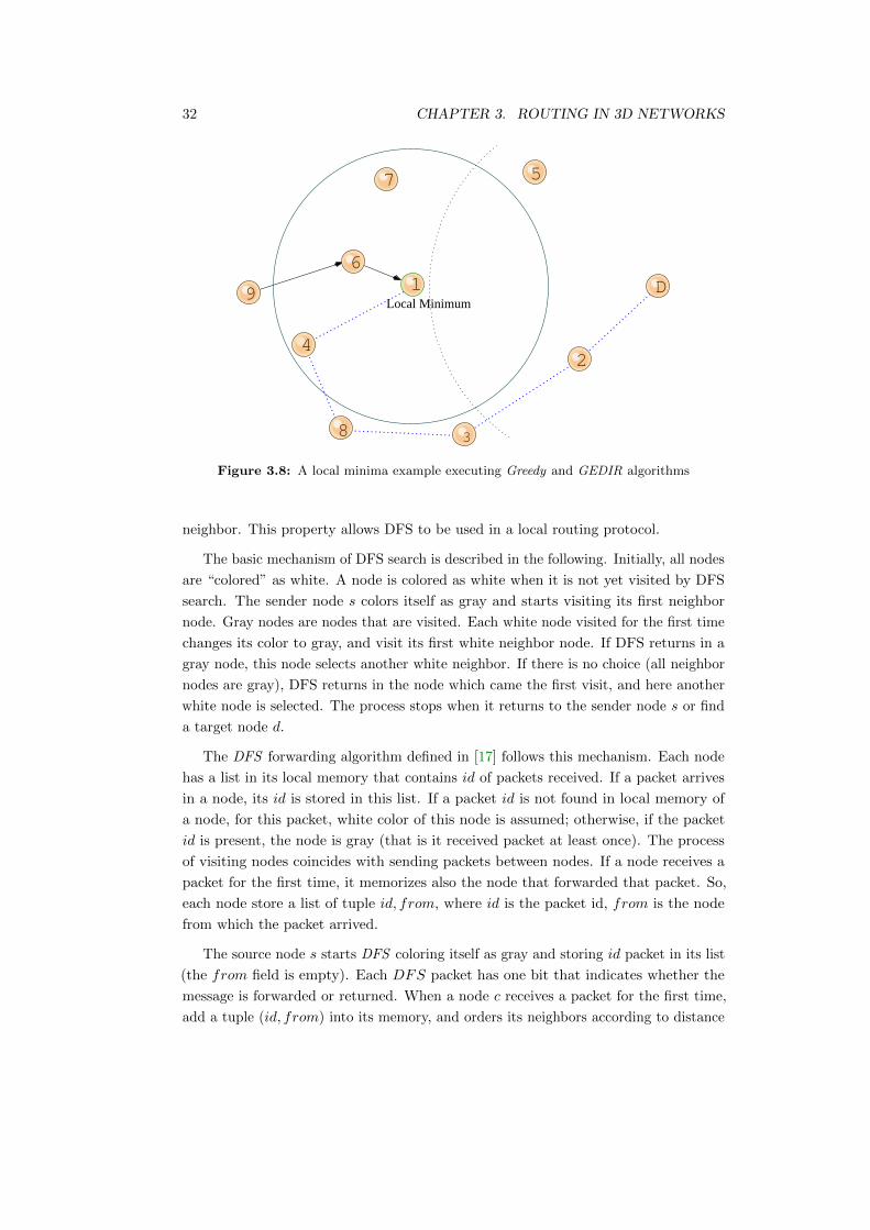
32 CHAPTER 3. ROUTING IN 3D NETWORKS
D1
3
2
5
9
4
8
7
6
Local Minimum
Figure 3.8: A local minima example executing Greedy and GEDIR algorithms
neighbor. This property allows DFS to be used in a local routing protocol.
The basic mechanism of DFS search is described in the following. Initially, all nodes
are “colored” as white. A node is colored as white when it is not yet visited by DFS
search. The sender node s colors itself as gray and starts visiting its first neighbor
node. Gray nodes are nodes that are visited. Each white node visited for the first time
changes its color to gray, and visit its first white neighbor node. If DFS returns in a
gray node, this node selects another white neighbor. If there is no choice (all neighbor
nodes are gray), DFS returns in the node which came the first visit, and here another
white node is selected. The process stops when it returns to the sender node s or find
a target node d.
The DFS forwarding algorithm defined in [17] follows this mechanism. Each node
has a list in its local memory that contains id of packets received. If a packet arrives
in a node, its id is stored in this list. If a packet id is not found in local memory of
a node, for this packet, white color of this node is assumed; otherwise, if the packet
id is present, the node is gray (that is it received packet at least once). The process
of visiting nodes coincides with sending packets between nodes. If a node receives a
packet for the first time, it memorizes also the node that forwarded that packet. So,
each node store a list of tuple id, from, where id is the packet id, from is the node
from which the packet arrived.
The source node s starts DFS coloring itself as gray and storing id packet in its list
(the from field is empty). Each DFS packet has one bit that indicates whether the
message is forwarded or returned. When a node c receives a packet for the first time,
add a tuple (id, from) into its memory, and orders its neighbors according to distance

3.3. SINGLE-PATH FORWARDING ALGORITHMS 33
5
d
2
3
s
1
4
Figure 3.9: Path performed by DFS. The node sequence is s− 2 − 3 − 1 − 2 − 1 − s− 1 −3 − 2 − 1 − 2 − s− 1 − s− 4 − 5 − d.
from destination d (this is the greedy method). The only node not to be taken into
account in the ordered list is node from that sent the packet to c. The packet is then
forwarded to the first choice u among neighbors (the first node chosen is the node that
is closest to the destination). If there is no choice, the packet is returned to from.
A gray node c, upon receiving forwarded packet from any node b, will reject the
packet immediately, returning it to b (returned message). A gray node b, upon receiving
a returned message from node c, will forward the message to the next choice e in its
sorted list of neighbors, if such a neighbor exists. If b has no more neighbors in its list,
the packet will be returned to the node from which sent the message for the first time
to b (memorized in packets list). To know which is the next node in the ordered list to
send the packet, an index L is used. L is the index, in the list, of the last neighbor
u selected for packet forwarding. When a new node has to be chosen, L is increased.
The pseudo code of DFS can be given in Algorithm 6.
DFS has one drawback: there are some situations in which the algorithm visit few
nodes many times, forming a sort of limited loop. Fig. 3.9 shows an example of this
case. The path performed by DFS is shown in the following (the arrows with f and r
represents respectively a forwarded packet sending and a returned packet sending).
sf→ 2
f→ 3f→ 1
f→ 2r→ 1
f→ sr→ 1
r→ 3r→ 2
f→ 1r→ 2
r→ sf→ 1
r→ sf→ 4
f→ 5f→ d
This basic DFS method can be improved in several ways. For example, an improve-
ment could be to memorize all the neighbor that sent a forwarded packet which was
then reject, in order to not choose them for next forwarding. However, this addition
increases the memory requirements.

34 CHAPTER 3. ROUTING IN 3D NETWORKS
Algorithm 6 One step of DFS algorithm
1: procedure DFS(c, d, from,N(c))
2: if c is source node then
3: L← 0
4: add in packet list entry < id,−, L >5: else
6: if forwarded packet then
7: if id packet is present in packet list then
8: set a returned packet
9: next← from
10: return next
11: else . packet arrived for the first time
12: L← 0
13: add in packet list entry < id, from,L >
14: sort N(c) (expcept from) according to distance from d as
u0, u1, ..., uk − 1
15: if L < k then
16: set a forward packet
17: next← uL
18: L+ +
19: return next
20: else
21: set a returned packet
22: next← from
23: return next
24: end if
25: end if
26: else . returned packet
27: sort N(c) (expcept from) according to distance from d as u0, u1, ..., uk−1
28: if L < k then
29: set a forward packet
30: next← uL
31: L+ +
32: return next
33: else if c is source node then
34: returnfail . source node is not connected to d
35: else
36: set a returned packet
37: next← from
38: return next
39: end if
40: end if
41: end if
42: end procedure

3.3. SINGLE-PATH FORWARDING ALGORITHMS 35
3.3.2 Randomized Progress-based Algorithms
Randomized-based forwarding algorithm, also called Random Walk algorithms, try to
solve the local minimum problem described in previous section, by choosing the next
node randomly from a subset of the current node’s neighbors that makes progress to
the destination. Already since 1984, some authors have tried to put the concepts of
randomization algorithms in order to avoid the emergence of loops: authors of [29]
study the case where a packet destined towards a destination node d in the network
are routed with equal probability towards one immediate neighboring node that lies
in the general direction of d; in [27] authors present examples of several situations
where Greedy and Compass algorithms fail, and then propose the Randomized Compass
Routing ; in [36] authors propose several variations of greedy and compass heuristics
with using randomization, combining them in various way. Routing algorithms that
use randomization are usually considered to fail when the number of hops in the path
computed so far exceeds a threshold value. The choice of this value is important because
determines the probability of reaching the destination and length of the path traveled
by algorithm: if threshold valued is little, the chances of reaching the destination are
few, if is great, the chances are many, but with a very large number of hops. A typical
value for the threshold is the number of nodes in the network graph, or multiple of
them. Performance of randomized algorithms, in terms of delivery rate, are much
better than deterministic algorithms in general, but they are worse in terms of path
dilation.
Random Compass
Random Compass is a first randomized algorithm proposed in [27]. In this method
the current node c choose a neighboring node, called ccw(c), that minimizes the
angle ∠dc{ccw(c)}, and a neighboring node, called cw(c), that minimizes the angle
∠{cw(c)cd}. ccw and cw refer respectively to counterclockwise and clockwise, that are
the respective directions of searching from line cd.
In [37] authors propose a set of randomized routing algorithms that uses various
methods. In this context, the most significant algorithms are considered in the following.
RCompass
In RCompass algorithm, d selects one neighbor u1 of c above the line cd such that
∠dcu1 is the smallest angle among all such neighbors, and one neighbor u2 of c below
the line cd such that ∠u2cd is the smallest angle among all such neighbors. Then it
choose the next node u uniformly at random from u1 and u2.
WeightedRCompass
WeightedRCompass algorithm selects u1 and u2 in the same way described in RCompass,
but the next node u is chosen from u1 and u2 with probability θ2(θ1+θ2) and θ1(θ1+θ2),
respectively.
Best2Compass
36 CHAPTER 3. ROUTING IN 3D NETWORKS
With Best2Compass algorithm u1 and u2 are selected in such a way that ∠dcu1 (or
∠u1cd) and ∠dcu2 (or ∠u2cd) are the two smallest such angles among all neighbors
of c. This method is different from RCompass in that the directions of the smallest
angles are not considered.
Best2Greedy
Best2Greedy algorithm selects u1 and u2 in such a way that they are the closest and
the second closest neighbors of c to the destination d.
3.3.2.1 3D extension of randomized algorithms
Extension of randomized algorithm is not trivial, because it is not obvious to choose the
best way to determine candidate neighbors. The reason is that in a three-dimensional
graph there is no concept of above and below a line passing from source to destination.
So, directly using of some algorithms, as RCompass or WeightedRCompass, that use a
line sd for reference, is not possible. Therefore, in [4] authors propose an extension for
the algorithms seen above, called by them AB algorithms (Above/Below), from 2D to
3D, that uses the concept of 3D planes. This new algorithm is called AB3D.
AB3D
AB3D is a randomized routing algorithms that uses three parameters for make for-
warding decisions. The first parameter is m, that indicates the number of possible
candidates, and can be 3 or 5. The second is R that is one of CM (as Compass),
GR (as Greedy) or MF (as Most Forward) and represent the strategy for choosing
candidate nodes. Similarly, the symbol S represents the probability weighting when
randomly choosing between more than one candidate neighbors and it is one of U , A
or D.
If the symbol S is U , then the next node is chosen uniformly at random from ni, that
is with probability:
PU (ni) =1
m.
If the symbol S is D then the next node is chosen from ni with probability:
PD(ni) =1− pi
p0 + ...+ pm-1, where pi = disti = dist(ni, d).
If the symbol S is A then the next node is chosen from ni with probability:
PA(ni) =1− pi
p0 + ...+ pm-1, where pi = θi = ∠nicd.
The steps of the algorithm are the following. The current node c selects a node n1
from its neighbors, chosen according to the method defined in R (CM , GR or MF ).
Define the plane PL1 identified by the three nodes s, d and n1. If m is 5, define also

3.3. SINGLE-PATH FORWARDING ALGORITHMS 37
S
n1
PL_1
PL_2D
Figure 3.10: In AB3D, plane PL1 passes through s, d and n1, plane PL2 is orthogonal to
PL1. Both planes contain the line sd.
the plane PL2 that is perpendicular to PL1 and passes through c and d, such that the
intersection line between the two planes is the line cd. Fig. 3.10 shows an example
of network graph and its subdivision with the two planes. Then, if the parameter m
is 3, AB3D select another two nodes, in addition to n1. One neighbor n2 is chosen
from the above of the plane PL1 according to R and one neighbor n3 is chosen from
the below of the plane PL1 according to R. If m is 5, in addition to n1, the algorithm
choose from N(c) four neighbors n2, n3, n4, n5 each one in one side of the four regions
that result from the intersection between PL1 and PL2. Once these candidates are
determined, node c selects one of these nodes randomly, according to the probability
weighting determined by S, and forwards the packet to the chosen node.
3.3.2.2 Unification of randomized algorithm - Random Walk
The algorithms seen above have a common mechanism: they choose m neighboring
nodes that satisfy a certain requirement and then one node is chosen among these
according to a certain probability (uniform or weighted). In this work, all these
algorithms are generalized in a single algorithm, called Random Walk (RW ) and that
accepts some parameters. Abdallah et al. in [4] and [5] calls this generic algorithm

38 CHAPTER 3. ROUTING IN 3D NETWORKS
AB, but does not include all the variants described in [37] (e.g. Best2Compass and
Best2Greedy can’t be defined by AB3D algorithm), then here a more general algorithm
that encompasses all and adds other variants is defined. Note that in RW, and obviously
in previous randomized algorithms, the greedy method does not maintain the status of
its failure condition, because it must be able to allow to go back, selecting also nodes
that have backward progress (GEDIR algorithm is used to choose the candidate nodes
in RW ). If the deterministic termination condition would be present, randomization
would not make sense. The pseudo code of RW can be given in Algorithm 7.
Random Walk
Random Walk (RW ) algorithm has four attributes, that are:
• m: are possible candidate neighbors to choose from N(c).
• R: is the name of progress-base algorithm used to choose the m candidates, and
it is one of R (Random), CM (Compass), GR (Greedy) or MF (most Forward),
as in AB3D.
• S: is used to represent the probability weighting when randomly choosing, and
it is one of U (Uniform), D (Distance) , A (Angle), PD (Projection Distance).
Probability weightings are defined as in AB3D.
• ab (above-below): is a boolean flag indicating whether to define the candidates
over and below the Plane PL1 (or even over and below the plane PL2, if m = 5),
or select candidates without considering the planes.
In the papers that propose randomized-based algorithms there is no explicit indication
of whether the previous node prev, the node that sent the packet at the previous step,
is chosen again by the current node c in the next step. Some tests show that the
performance of RW improve when the previous node is not included in the candidates
list. So, our implementation of RW assumes that the previous node prev is not
considered (of course it is considered as the only neighbor of c).
In the simulations of this thesis, only this algorithm with different parameters is
performed. In table 3.1, RW is associated with most of the algorithms defined in [4, 5,
27, 37].
3.3.3 Face-based algorithms
Face, a.k.a, Perimeter forwarding method has been proposed first time in [12] and
optimized in [26]. This method is a typical planar graph technique which involves
walking adjacent faces using the right-hand rule and it is the first geographic routing
algorithm that guarantee a delivery rate of 100% in 2D network graphs. Position
information can be used to extract a planar subgraph that is a graph that contains

3.3. SINGLE-PATH FORWARDING ALGORITHMS 39
Algorithm 7 One step of Random Walk algorithm
1: procedure RW(c, d, p,N(c),m,R, S, ab)
2: if ab = Y ES then
3: sump ← 0
4: for i← 0 to n do
5: ni ← R(c, d,N(c))
6: N(c)← N(c) \ ni7: pi ← S(ni, c, d)
8: sump ← sump + pi
9: if N(c) is empty then
10: break
11: end if
12: end for
13: next←choose one of ni with probability equal (1− pi)/sump
14: else . ab = NO
15: if m = 3 then
16: n1 ← R(c, d,N(c))
17: c computes the plane Pln1
18: above← all the nodes above Pln1 from N(c)
19: below ← all the nodes below Pln1 from N(c)
20: n2 ← R(c, d, above)
21: n3 ← R(c, d, below)
22: sump ← 0
23: for i← 1 to 3 do
24: pi ← S(ni, c, d)
25: sump ← sump + pi
26: end for
27: else if m = 5 then
28: c computes the plane Pln2 ortogonal to plane Pln1
29: aboveo ← all the nodes above Pln1 and above Pln2 from N(c)
30: abovee ← all the nodes above Pln1 and below Pln2 from N(c)
31: belowo ← all the nodes below Pln1 and above Pln2 from N(c)
32: belowe ← all the nodes below Pln1 and below Pln2 from N(c)
33: n2 ← R(c, d, aboveo)
34: n3 ← R(c, d, abovee)
35: n4 ← R(c, d, belowo)
36: n5 ← R(c, d, belowe)
37: sump ← 0
38: for i← 1 to 5 do
39: pi ← S(ni, c, d)
40: sump ← sump + pi
41: end for
42: end if
43: next←choose one of ni with probability equal (1− pi)/sump
44: end if
45: return next
46: end procedure

40 CHAPTER 3. ROUTING IN 3D NETWORKS
Table 3.1: List of randomized algorithm and their attribute values in RW.
Name Attribute values in RW
RCompass (2D) RW(3, CM, U, ab = YES)
WeightedRCompass (2D) RW(3, CM, A, = YES)
Best2Compass (2D) RW(3, CM, U, ab = NO)
Best2Greedy (2D) RW(3, GR, U, ab = NO)
AB3D(R, S) RW(3, R, S, ab = YES)
AB3D(m, R, S) RW(m, R, S, ab = YES)
faces whose corners are the terminal node. So that routing can be performed on
the faces of this subgraph. This type of algorithms suffers from the problem of a
high traffic. Some alternatives that seek to hybridize this algorithm with the first
progress-based algorithms seen so far, such as Greedy, have been proposed. These
hybrids sacrifice a bit of the delivery rate for the reduction of traffic. For example GFG
(Greedy-Face-Greedy), also called Greedy Perimeter Stateless Routing (GPSR) (in [7],
with little enhancements), is an hybrid algorithm that start from greedy approach until
the packet find a local minimum, then it change and switch to Face algorithm, until to
find a node closer to that in which one was blocked, and then return to greedy. GFG
is described in 3.3.4.
3.3.3.1 Connected Planar Sub-graph
Face algorithm work by finding a connected planar sub-graph of UDG and then
applying routing algorithm for planar graph on this sub-graph. In this section we
describe a distributed algorithm for extracting a connected planar sub-graph from
UDG, called Gabriel Graph (GG)1. Each node can run this algorithm and the only
information needed is the position of each of its neighbors. Let disk(u, v) be the disk
with diameter dist(u, v). Then, the Gabriel graph GG of a graph G, denoted by GG(G)
is a geometric graph in which the edge (u, v) is present if and only if disk(u, v) contains
no other points of G. Then a Gabriel Graph does not contains two edge that crosses,
and [21] demonstrates that if we apply this algorithm to each vertex of G then the
resulting graph is connected. Fig. 3.11 show an example of graph planarization.
Face
In [26], two algorithm that make routing are proposed, Face1 and Face2. In this
work, only Face2 algorithm is considered, that is more optimized than Face1. Face2
algorithm starts by extracting the GG sub-graph from UDG. Then the packet are
routed over the faces of GG, which are intersected by the line between the source
1Another sub-graph of G is Relative Neighbourhood Graph (RNG(G)), in which each node u keeps
its outgoing edge uv if circles with centers u and v and radii |uv| contains no other node than v. In
this thesis the RNG will not be considered

3.3. SINGLE-PATH FORWARDING ALGORITHMS 41
(a) (b)
Figure 3.11: Planarization of a graph (a) to extract the GG sub-graph (b).
and the destination, sd, using the right-hand rule. The boundary of current face f is
traversed in the counterclockwise direction, unless the current edge crosses sd at an
intersection point p. At this point, the algorithm switches to the next face sharing the
edge (that contains the previously intersection point) and continues with the right-hand
rule. This process is repeated until the packet arrives to the destination. In Fig. 3.12),
an example of Face2 behavior are shown. Node x uses right hand rule to forward
packet to node 5, then to node 9. At this point, for right hand rule, the next node
should be 2, but link between 9 and 2 crosses the line xd, and the same happens with
nodes 8 and 3. So, the next node is 4. In Algorithm 8 the pseudo code of Face2 is
reported.
Algorithm 8 Face2 algorithm
1: p← s
2: while p 6= d do
3: let f be the face of G with p on its boundary that intersects (p, t)
4: traverse f until reaching an edge (u, v) that intersects (p, t) at some point p′ 6= p
5: p← p′
6: end while
3.3.3.2 3D extension of Face routing algorithms
In 3D graphs, extracting a straight line planar graph is impossible because the line
sd does not determine the faces in this 3D graph. So, the notion of planarization and
traversing faces do not exist. Thus, Face algorithm cannot directly applicable on a 3D
graphs. Kao et al. in [15] propose a heuristic that adapt the face strategy using the
projected graph to deal the problem. This approach presents two problems: first, this
method doesn’t guaranteed the delivery rate, because in many cases the projection of

42 CHAPTER 3. ROUTING IN 3D NETWORKS
5
2
D
4
8
3
9
c
6
7
Figure 3.12: Forwarding steps of Face2 algorithm.
the nodes in a plan may generate cycles from which Face algorithm can not get out,
and second, the planar graph cannot be extracted from the projected graph using only
its local information before projection.
However, the experiments show that the delivery rate is significantly better than
the other progress-based routing algorithms. Moreover, in [12] it is shown that if the
2D network of nodes forms a layer of a thickness of not larger than 1/sqrt(2) times
the range of a node, then there exists a particular algorithm based on face strategy
which can guarantee a delivery rate to 100%. The following is a treatment of main 3D
face routing algorithms proposed in recent years.
Projective face
The first extension of Face algorithm in 3D space provides using two orthogonal planes
intersected to the line connecting source and destination. In [15] authors propose
Projected Face, that proceed as follows. The points of the networks are firstly projected
onto one plane that contains the line sd, with third point chosen randomly. Face
algorithm is performed on this projected graph. If the routing fails, the points are
then projected onto the second plane, that is orthogonal to the first plane and also
contains the line sd. Face algorithm is again performed. Fig. 3.15 shows an example of
planes configuration in Projective Face. Note that, in this case (and in all the following
algorithms), since the delivery rate is not guaranteed, the algorithm needs a local
threshold value, TTLF (Time To Live Face), in order to terminate the algorithm in
case it not reached the destination. This is necessary because the algorithm can get
stuck in a loop. More precisely, in this version of algorithm, TTLF counter is started
twice, once for the first plane and one for the orthogonal plane, obtaining a global

3.3. SINGLE-PATH FORWARDING ALGORITHMS 43
Projection Plane
Figure 3.13: Nodes projected on a plane
Figure 3.14: Cross link in red circle

44 CHAPTER 3. ROUTING IN 3D NETWORKS
S
D
Casual Point
Figure 3.15: Computing of a plane with Projective face algorithm
threshold value ,TTL, at most 2 ∗ TTLF . As discussed in the next chapter, this first
extension, in some cases, provides a delivery rate greater than 90%, though suffering a
very high path dilation.
CoordinateFace(3)
CoordinateFace(3) (CFace(3)), proposed in [4], uses another set of projection planes,
that is the planes xy, xz and yz for the projection of the nodes. CFace(3) works
as follow. All nodes are projected on the first xy plane (node.z = 0) and then the
face routing is started on the projected graph. If the packet does not arrive at the
destination (TTLF has expired) , original coordinate of all nodes are projected in
xz plane (node.y = 0) and face routing is again performed. If again the packet does
not arrive to the destination, original coordinate of all nodes are projected on yz
plane (node.x = 0) and face routing is again performed. If the packet does not arrive
with this last plane, algorithm fails. Fig. 3.16 shows all the three projections on the
coordinate planes. Note that, in this algorithm, TTL is at most 3 ∗ TTLF . As we will
see, the delivery rate is typically greater greater than that of the Projective face, but
with a greater path dilation. A pseudo code of CFace(3) is shown in Algorithm 9.
Adaptive Least-Squares Projective Face
Authors of [14] proposes three heuristics to modify and improve Projective Face
algorithm. The new algorithm is called Adaptive Least-Squares Projective Face, (ALSP

3.3. SINGLE-PATH FORWARDING ALGORITHMS 45
(a) (b)
(c) (d)
Figure 3.16: Projection of graph nodes (a) on the three planes xy (b), xz (c) and yz (d) in
CFace(3) algorithm.

46 CHAPTER 3. ROUTING IN 3D NETWORKS
Algorithm 9 CFace(3) algorithm
1: c← s
2: Compute the projected graph on the xy plane (z = 0)
3: while pre-set TTLF is not reached do
4: Perform Face algorithm step
5: if d is reached then
6: return true
7: end if
8: end while
9: Compute the projected graph on the xz plane (y = 0)
10: while pre-set TTLF is not reached do
11: Perform Face algorithm step
12: if d is reached then
13: return true
14: end if
15: end while
16: Compute the projected graph on the yz plane (x = 0)
17: while pre-set TTLF is not reached do
18: Perform Face algorithm step
19: if d is reached then
20: return true
21: end if
22: end while
23: return fail

3.3. SINGLE-PATH FORWARDING ALGORITHMS 47
Face). The three heuristics are:
• Least-Squares Projection (LSP) Plane;
• Adaptive Behavior Scale (ABS);
• Multi-Projection-Plane Strategy.
In the Projective Face, a third point is chosen randomly, together with the source and
the destination points, to compute the first projection plane. Instead, ALSP Face
choose the third point adopting a mathematical optimization technique (first heuristic)
for finding the best fitting plane to the set of neighbor nodes: using the current node,
its neighbors up to two hops away, and the destination node, the initial projection
plane is determined by using least-squares error minimization of the distance of the
nodes to the plane, minimizing the sum
m∑i=1
(ri)2
where ri is the Euclidean distance from a point i to its perpendicularly projected point
in the least-squares projection plane (LSP plane), as seen in Fig. 3.17. To maintain
the local characteristic of the routing algorithm, authors propose that only the source,
destination and the neighboring nodes within the 2-hops scope of the current node be
selected as the set of points for computing the least projection plane 2 Then, nodes are
projected to this plane and Face routing is performed. This LSP plane aim to have
a less distorted projected graph so that the number of crossing edges can potentially
be reduces. The second heuristic defines a parameter called Adaptive Behavior Scale
(ABS) that is used to determine when recalculate the LSP plane, in order to ensure
that the plan is always appropriate for the current node. Third heuristic uses a set of
Ns projection planes arranged in a fixed order about an axis. The algorithm switches
between these planes, following the order, to disrupt any looping that may occur during
routing. In Algorithm 10 ALSP Face is written in pseudo code.
In [14] it is said that by performing the face routing on the additional projection
plane, there is a significant increase in the delivery rate. Therefore, third heuristic tries
to increase the number of projection planes. But this reasoning is true only up to a
certain point: if it is true that the delivery rate is slightly increased, it is also true that
the path followed by the packet becomes enormously long, because, for each projection
plane, the threshold value (here, TTLF ) is reset to the its pre-set value. Such a high
traffic for only one packet might not be acceptable in real world. Then it is not clear
So, this thesis consider the third heuristic using only two additional planes, chosen as
in Projective Face.
2for simplicity of implementation, in this work the 1-hop scope of current node was used for LSP
plane computing

48 CHAPTER 3. ROUTING IN 3D NETWORKS
LSP
Figure 3.17: 2D graphic representation of computing Least-Squares Projection (LSP) plane,
as the first projection plane.
Algorithm 10 Adaptive Least-Squares Projective Face algorithm, refering to [14]
adapted to this thesis.
1: Input The source node (s), the destination node (d) and a 3D geometric graph.
2: Output return true if the delivery is successful else return false.
3: c← s
4: while pre-set TTLF is not reached do
5: Compute LSP plane using position of c, t and the 1-hop neighbors of c.
6: Compute the projected graph on the LSP plane.
7: while pre-set ABS is not reached do
8: Perform a 2D Face routing step.
9: if t is reached then
10: return true
11: end if
12: end while
13: end while
14: while pre-set number of projection planes Ns is reached do
15: Compute the next projection plane.
16: Compute the projected graph on the plane.
17: while pre-set TTLF is not reached do
18: Perform a 2D Face routing step.
19: if t is reached then
20: return true
21: end if
22: end while
23: end while
24: return false

3.3. SINGLE-PATH FORWARDING ALGORITHMS 49
3.3.4 3D Hybrid Algorithms
In this section we will discuss a set of 3D hybrid algorithms that have been proposed
to solve some disadvantages of the algorithms previously seen. These algorithms work
at different times using one of two algorithmic methods in alternate way (for example
greedy phase and face phase, as in GFG). Initially the algorithm begins with a method,
then, if a certain condition is satisfied (or not), the algorithm switches to the other
method. The three classic combinations that we’ll see, will be the combination of two
algorithms that are part of the three categories seen above: progress-based/randomize-
based, progress-based/face-based, randomized-based/face-based. Typically the primary
stage is a progress-based strategy, while the second, also called recovery phase, a is
random-based or face-based strategy. All the algorithms treated follows set the packet
with two modalities, which represent the two used methods.
Greedy-Random-Greedy
Greedy-Random-Greedy (GRG) algorithm belongs to progress-based/randomized-based
class, and uses Greedy as the primary stage and a randomized algorithm, such as
Random Walk, as a recovery strategy. Unlike the recovery strategy based on face
routing, randomization strategy is able to obtain a delivery rate similar but with a
much lower path dilation. The general idea of this algorithm is the following: the
algorithm starts with proceeding the greedy phase until it find a local minimum c.
At this point, it will switch to random phase, as recovery strategy, where the node c
randomly selects one of its neighboring nodes, using probability distributions defined
in RandomWalk. In this case, it is very likely that the next node chosen u is not a
local minimum, then resumes the greedy forwarding. If the node u is another local
minimum, is again the recovery phase.
Greedy-Face-Greedy
Greedy-Face-Greedy algorithm (GFG), also defined as Greedy Perimeter Stateless
Routing algorithm (GPSR) for 2D networks, uses a combination of greedy method
with face method. With GFG, a flag is stored in data packet. This flag can be set
into greedy-mode and face-mode (or perimeter-mode), indicating whether the packet
is forwarded with Greedy or Face algorithm. The algorithm starts from s with Greedy,
setting the packet into greedy-mode and forwarding it. A node that receives a greedy-
mode packet, searches from its neighbors the node that is closest to the destination.
If this neighbor exists, the current node forwards the packet to this, otherwise marks
the packet into perimeter-mode. GFG algorithm forwards the perimeter-mode packets
performing the same planar graph as the Face2 algorithm. Moreover, when a packet
enters in perimeter-mode at node x, GFG set the line xd as a reference line to the
crossing with the faces and records in the packet the location of x as the node when
greedy forwarding mode failed. This information is used at next hops to determine
whether and when the packet can be returned to greedy-mode: upon receiving a
perimeter-mode packet, the current node c first compare the location of x stored in

50 CHAPTER 3. ROUTING IN 3D NETWORKS
D9
4
8
3
2
c
5
6
7
Local Minimum
Figure 3.18: Example of GFG algorithm. Green arrows represents packet forwarding in
greedy-mode, blue arrows are represents packet forwarding in face-mode.
the packet with the forwarding node’s location. GFG returns in greedy-mode if the
distance from the forwarding node to d is less than the distance from x to d. In this
case the packet is set into greedy-mode and algorithm continue greedy progress towards
the destination. Fig. 3.18 shows an example, where the packet travels nodes 9, 6 and
c in greedy-mode (the green path), stopping at node c, that is the local minimum.
Then, from node c the face-mode is started, and forwards the packet on progressively
closer faces of the planar graph, each of which is crossed by the line cd. The packet
reaches nodes 7, 8 and 5 (the blue path). Node 5 is closest to the destination d than c,
so the packet can be returned to greedy-mode and reaches destination d (the second
green path). GFG has the same guaranteed delivery rate (100%), but reduces the
number of hops traveled compared to pure face routing strategy. A pseudo code of
GFG algorithm is given in Algorithm 11.
RW-CFace(1)-RW
This algorithm, initially conceived in [4] as AB3D-CFace(1)-AB3D, starts with RW
algorithm. Once the local threshold TTLR is passed and the algorithm reaches a local
minimum, it switches to CFace(1). CFace(1) traverses one projective plane, which is
chosen randomly from the xy, yz, or xz planes, starting from the node in which the
algorithm is switched. At this point, TTLF is initialized to 0 and CFace(1) restarts.
If the destination is not reached during this phase and TTLF is passed (a looping
occurs), the algorithm goes back to RW and TTLR restarts at 0.

3.3. SINGLE-PATH FORWARDING ALGORITHMS 51
Algorithm 11 Greedy-Face-Greedy algorithm
1: c← s
2: while pre-set TTL is not reached do
3: while c is not a local minimum do
4: Perform Greedy algorithm step
5: if d is reached then
6: return true
7: end if
8: end while
9: let p be the closest node to d before turn on face phase
10: p← c
11: while dist(p, d) <= dist(c, d) do
12: Perform Face algorithm step
13: if d is reached then
14: return true
15: end if
16: if pre-set TTLF is reached then
17: return fail
18: end if
19: end while
20: end while

52 CHAPTER 3. ROUTING IN 3D NETWORKS
RW-CFace(3)
This algorithm starts as RW-CFace(1)-RW, but instead of going back to RW if the
phase in a projective plane fails, RW-CFace(3) tries the other two projective planes,
define as in CFace(3). This algorithm starts with RW stage and if the destination
is not reached and TTLR is passed, the algorithm switches to CFace(3) using the
first xy plane. Again if a loop occurred (TTLF is reached), it switch to yz plane, and
finally the same process is make for xz plane.
3.4 Multi-path Forwarding Algorithms
Flooding is a routing protocol used by routers to forward an incoming packet on all lines
except the one it came from. Multi-path strategy uses a partial flooding mechanism to
deliver the packet to the destination. With partial flooding each node may forward
the packet to more than one of the neighbors. Flooding-based algorithms present the
problem of packet redundancy: a node can receive a packet for the second time, or
even several times, resulting in a very high traffic if it does not have a mechanism to
recognize and eliminate these duplicate packets. Moreover, this situation, can lead to
an infinite sending of packets. To avoid infinite sending of duplicate packets there are
two shrewdness:
• Jump count: the package has a counter to be decremented when a new router is
crossed. Ideally, the value of this counter should be the same as the shortest path
between source and destination, but not knowing the topology of the network, it
can be assigned a value equal to the diameter of the network, or the number of
nodes in the network.
• Store sequence number: this strategy need a sort of memory mechanism, that
store in a sequence number table the sequence number of the packets arriving
from all the neighbors, for some time. If any packet reach a node, the node check
in the sequence number table if the sequence number of the packet is present.
If so, it just ignores it and does not forward it, otherwise insert the sequence
number within the table and forwards the packet.
In this thesis a partial flooding strategy (also called restricted directional flooding) is
considered. A partial flooding try to send packet to more than one of the neighbors
that are located closer to the destination, than the forwarding node itself. Examples
of routing algorithms that use this strategy are Distance Routing Effect Algorithm
for Mobility (DREAM ) and Location-Aided Routing (LAR). We consider only LAR
algorithm for its 3D extension, comparison and hybridizing it with RW algorithm.

3.4. MULTI-PATH FORWARDING ALGORITHMS 53
s
d
Figure 3.19: Performing of LAR algorithm. Packets are forwarded only to nodes that are
located within the defined area.
LAR
This algorithm uses the position information of nodes to restrict the flooding process.
LAR strategy was created first time in reactive topology-based algorithm, to reduce
the sending area of Request Message (RREQ) during the route discovery phase. With
the available information of source node and destination node positions, the flooding
area is (in 2D) a minimum size rectangle with disk(s, r) in one corner and the expected
zone in the other corner. Expected zone, in the original definition [38], is a circle
around d of radius equal to vmax ∗ (t1 − t0) where t1 is the current time, t0 is the time
stamp of the position information that c has about d, and vmax is the maximum speed
of the node in the network. In our case, since we analyze static scenarios (vmax = 0),
the expected zone is disk(d, r). Figure 3.19 shows an example of packet forwarding in
LAR area, depending on position of source and destination.
3.4.0.1 3D extension of partial flooding algorithms
3D extension of this class of algorithms does not require considerable changes. It is
sufficient extend in three dimensional space the flooding areas in which packets can be
forwarded.

54 CHAPTER 3. ROUTING IN 3D NETWORKS
LAR 3D
In the extension of LAR algorithm in 3D space, with three-dimensional coordinates of
source and destination positions, the source node computes the expected zone for d,
which is a sphere around d of radius equal to vmax ∗ (t1 − t0) where t1 is the current
time, t0 is the time stamp of the position information that c has about d, and vmax is
the maximum speed of the node in the network. This zone is used to define the 3D
flooding area, which is the minimum size rectangular box with ball(s, r) in one corner
and the expected zone in the opposite corner. In our case, since we analyze static
scenarios (vmax = 0), the expected zone is ball(d, r).
RW-LAR
RW-LAR was proposed in [5] and hybridize Random Walk with LAR. This algorithm
try to reduce the high path dilation of LAR algorithm. All the combinations in
RW-LAR use the same partitions as in Random Walk algorithm. The difference is that,
while RW select only one of the m candidates chosen from the neighborhood, RW-LAR
sends the packet to all those selected candidates which are within the rectangular box
defined as in LAR.

Chapter 4
Simulation Environment
This chapter provides some insights on the simulation environment used for the experi-
mentation. In addition, we provide some common settings related to the simulations
such as the orchestration of the simulation scenario.
4.1 Network Simulator 2 (NS-2)
Network Simulator 2, widely known as NS-2, is an object-oriented, discrete event-driven
simulator tool that is useful in studying the dynamic networks. This simulator can
simulate wired as well as wireless network and communication protocols (e.g., routing
algorithms, TCP, UDP). In general, NS-2 provides users with a way of specifying such
network protocols and simulating their corresponding behaviour. Since it was born, in
1989, NS-2 has gradually gained great popularity and, ever since, several revolutions
and revision have marked the growing maturity of the tool, with the contribution of
many users in the field and, since 1995, with support of DARPA (Defence Advanced
Research Project Agency). In NS-2, many network protocols are implemented, located
in the different logical network layers:
• Phy/MAC layer (links, CSMA/CD, etc).
• Network layer (AODV, DSR, etc).
• Transport layer (TCP, UDP, etc).
• Application layer (web, telnet, ftp, etc).
55

56 CHAPTER 4. SIMULATION ENVIRONMENT
3
Linkage Between OTcl and C++ in NS2
NS2 is an object oriented simulator written in OTcl and C++ languages.While OTcl acts as the frontend (i.e., user interface), C++ acts as the back-end running the actual simulation (Fig. 3.1). As can be seen from Fig. 3.1,class hierarchies of both languages can be either standalone or linked togetherusing an OTcl/C++ interface called TclCL [15]. There are two types of classesin each domain. The first type includes classes which are linked between theC++ and OTcl domains. In the literature, these OTcl and C++ class hierar-chies are referred to as the interpreted hierarchy and the compiled hierarchy,respectively. The second type includes OTcl and C++ classes which are notlinked together. These classes are neither a part of the interpreted hierarchynor a part of compiled hierarchy. This chapter discusses how OTcl and C++languages constitute NS2.
C++ class
class class class
class class
OTclclass
class classclass
class class
one-to-one correspondence
The interpretedhierarchy
The compiledhierarchy
Fig. 3.1. Two language structure of NS2 [12]. Class hierarchies in both the lan-guages may be standalone or linked together. OTcl and C++ class hierarchies whichare linked together are called the interpreted hierarchy and the compiled hierarchy,respectively.
Written in C++, TclCL consists of the following six main classes:
• Class Tcl provides methods to access the interpreted hierarchy (from thecompiled hierarchy; Defined in files ˜tclcl/tclcl.h and ˜tclcl/Tcl.cc).
T. Issariyakul, E. Hossain, Introduction to Network Simulator NS2,
DOI: 10.1007/978-0-387-71760-9 3, c© Springer Science+Business Media, LLC 2009
Figure 4.1: Two language structure of NS-2. Class hierarchies in both the languages (C++
and OTcl) may be standalone or linked together. OTcl class hierarchy is the
interpreted hierarchy and C++ class hiearchy is the compiled hierarchy
4.1.1 Why use NS-2?
NS-2 is a free open source common simulator with support for simulations of a
large number of protocols and also provides opportunity to study large-scale protocol
interaction in a controlled environment. Moreover, NS-2 allows users to extend the code
by implementing their own protocols. In fact, in the work of this thesis, a new routing
agent module has been implement to add new georouting functionalities. However,
NS-2 has certain disadvantages, such as NS’s dual language implementation is proving
to be a barrier to some developers. But increasing awareness among the researchers
along with the other tools like tutorials, manuals and mailing lists have improved the
situation.
4.1.2 Basic architecture
NS-2 is written in C++ and Object-oriented Tool Command Language (OTcl), that split
the programming model. So, the implementation of this model is distributed between
two languages, in order to provide adequate flexibility without losing performance.
While the C++ defines the internal mechanism of the simulation and all the objects
of network communication (nodes, packets, links), the OTcl sets up simulation by
assembling and configuring the objects as well as scheduling discrete events. These
two languages are linked using TclCL, mapping variables (instvars) and functions
(instprocs), in the OTcl domains, into C++ objects. In this way it is possible to run
simulations without the need to recompile at every change, being able to act directly
in the script, which is then translated from OTcl in C++ (see Fig. 4.1). The choice of
using two languages instead of one comes from the fact that C++ is faster in execution,
but less convenient to change; to the contrary, OTcl has lower performance, but it can
be changed very quickly, which is ideal for touch-ups configurations.
NS-2 can be invoked by executing NS command from the shell environment, followed

4.2. EXPERIMENTAL SCENARIO 57
20 2 Introduction to Network Simulator 2
examples for setting up basic NS2 simulation. A comprehensive list of NS2codes contributed by researchers can be found in [13]. These introductoryonline resources would be helpful in understanding the material presented inthis book.
In this chapter an introduction to NS2 is provided. In particular, Sec-tion 2.2 presents the basic architecture of NS2. The information on NS2installation is given in Section 2.3. Section 2.4 shows NS2 directories andconventions. Section 2.5 shows the main steps in NS2 simulation. A simplesimulation example is given in Section 2.6. Section 2.7 describes how to includeC++ modules in NS2. Finally, Section 2.8 concludes the chapter.
2.2 Basic Architecture
Figure 2.1 shows the basic architecture of NS2. NS2 provides users with anexecutable command ns which takes on input argument, the name of a Tclsimulation scripting file. Users are feeding the name of a Tcl simulation script(which sets up a simulation) as an input argument of an NS2 executablecommand ns. In most cases, a simulation trace file is created, and is used toplot graph and/or to create animation.
NS2 consists of two key languages: C++ and Object-oriented Tool Com-mand Language (OTcl). While the C++ defines the internal mechanism (i.e.,a backend) of the simulation objects, the OTcl sets up simulation by assem-bling and configuring the objects as well as scheduling discrete events (i.e., afrontend). The C++ and the OTcl are linked together using TclCL. Mappedto a C++ object, variables in the OTcl domains are sometimes referred to ashandles. Conceptually, a handle (e.g., n as a Node handle) is just a string (e.g.,_o10) in the OTcl domain, and does not contain any functionality. Instead, thefunctionality (e.g., receiving a packet) is defined in the mapped C++ object(e.g., of class Connector). In the OTcl domain, a handle acts as a frontendwhich interacts with users and other OTcl objects. It may defines its ownprocedures and variables to facilitate the interaction. Note that the memberprocedures and variables in the OTcl domain are called instance procedures
SimulationObjects
Simulation Objects
TclCL
C++ OTcl
NS2 Shell Executable Command (ns)
TclSimulation
Script
SimulationTraceFile
NAM(Animation)
Xgraph(Plotting)
Fig. 2.1. Basic architecture of NS.Figure 4.2: Basic architecture of NS-2
by a Tcl script, that represents the simulation scenario. A scenario script, typically,
includes the definition of the network topology, the type of terminals, the active flows,
the type of connection between nodes (wired or wireless), the movement of the nodes,
and more. After simulation, NS-2 outputs either text-based simulation results. To
interpreter these results graphically and interactively, tool such as NAM (Network
AniMator) and XGraph are used. Fig. 4.2 shows the basic architecture of NS-2 and
all its steps.
In Network Simulator 2 physical activities are translated to events, that are queued
and processed in the order of their scheduled occurrences. The scheduler maintains the
chain of events and simulation (virtual) time. At runtime, it moves along the chain,
and dispaches one event after another. Since there is only one chain of events in a
simulation, there is exactly one Scheduler object in a simulation. NS-2 supports four
types of schedulers: List Scheduler, Heap Scheduler, Calendar Scheduler (default) and
Real-time Scheduler.
4.2 Experimental Scenario
A 3D MANET consists of n hosts located at different positions, at different altitudes
and connected between them through wireless links. Many of the works considered in
this thesis, have simulated their proposal on a scenario that is not very realistic. For
example, a typical scenario reproduced is a networks of 75 nodes inside a cube with
sides of length 100 units, and each node has a transmission range of 25 units. Possible
real networks contain a higher number of terminals, in a much larger structure than a
cube of side 100. In fact, many real-world applications are based on longer distances,
e.g, tactical or environmental disaster scenarios which need to cover a vast territory.
The basic feature of the simulation scenario involves the random placement of n nodes

58 CHAPTER 4. SIMULATION ENVIRONMENT
in a three-dimensional space, especially inside a cube of 500 units of side length. In
this work one unit is associated to a one meter in real world. This area size is closer to
the real typical area sizes.
Another common choice that many researchers have adopted in their work is to
start with the calculation of all connected components in the graph (LCC), then select
the largest connected component to perform the routing algorithms. This method can
creates considerable results as, declaring to position n nodes and then taking the LCC,
each different simulation is started with a different number of nodes involved, more
precisely nLCC ≤ n. This approach is not flexible when we are interested in studying
the impact of node density in the performance metrics of interest.
In this work each graph is generated with a set of nodes placed in the space,
constituting a connected ad-hoc network wherein between each pair of nodes exists a
least one path and all the nodes are connected. To do this, the Dijkstra shortest path
algorithm is used. In this regard, each graph is generated in the following steps:
1. All the n nodes are inserted in a list Q.
2. Every node in the list Q si randomly placed in a position (xi, yi, zi) within a
cube of side length N .
3. Starting from a defined node u (e.g., node 1) a Dijkstra algorithm is launched for
evaluate which nodes are connected to u. Each node that the algorithm meets is
removed, if any, from the list Q.
4. If Q is not empty, return to step 2.
In this way, each graph has always all n connected nodes, without leaving any node,
or group of nodes, stayed to itself, which would have not reason to exist in the graph.
For simplify the simulation, it is assumed that the nodes are not moving in space,
getting an ad-hoc static network. This choice depends on the necessity of having to
consider some initial essential parameters for the comparison (as the minimum path)
calculated in generation of graphs, that they would change with the addition of mobility,
not allowing a more precise analysis of the results. This slightly sacrifices the faithful
reproduction of reality, but it is easy to imagine many scenarios of application in which
sensor, drones, etc., are arranged in a space area to form an ad-hoc network, finally
settled (or at most moving for a few meters). For a more comprehensive comparison,
it is chosen to perform all the algorithms in networks with a variable number n of
nodes, in particular n = {50, 100, 150, 200}, in order to evaluate the behavior of those
algorithms varying the size of network. A different number of nodes within a cube
of equal size causes a change in the density of nodes themselves, therefore causing
a variation in the number of the average neighbors for each node. This feature has
highlighted some aspects, first including the different results that algorithms have
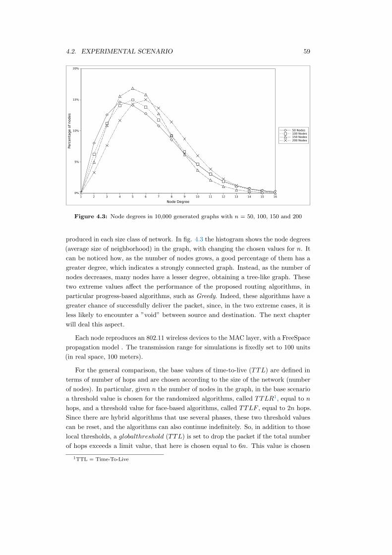
4.2. EXPERIMENTAL SCENARIO 59
1 2 3 4 5 6 7 8 9 10 11 12 13 14 15 16
Node Degree
0%
5%
10%
15%
20%Perc
enta
ge o
f nodes
50 Nodes
100 Nodes
150 Nodes
200 Nodes
Figure 4.3: Node degrees in 10,000 generated graphs with n = 50, 100, 150 and 200
produced in each size class of network. In fig. 4.3 the histogram shows the node degrees
(average size of neighborhood) in the graph, with changing the chosen values for n. It
can be noticed how, as the number of nodes grows, a good percentage of them has a
greater degree, which indicates a strongly connected graph. Instead, as the number of
nodes decreases, many nodes have a lesser degree, obtaining a tree-like graph. These
two extreme values affect the performance of the proposed routing algorithms, in
particular progress-based algorithms, such as Greedy. Indeed, these algorithms have a
greater chance of successfully deliver the packet, since, in the two extreme cases, it is
less likely to encounter a ”void” between source and destination. The next chapter
will deal this aspect.
Each node reproduces an 802.11 wireless devices to the MAC layer, with a FreeSpace
propagation model . The transmission range for simulations is fixedly set to 100 units
(in real space, 100 meters).
For the general comparison, the base values of time-to-live (TTL) are defined in
terms of number of hops and are chosen according to the size of the network (number
of nodes). In particular, given n the number of nodes in the graph, in the base scenario
a threshold value is chosen for the randomized algorithms, called TTLR1, equal to n
hops, and a threshold value for face-based algorithms, called TTLF , equal to 2n hops.
Since there are hybrid algorithms that use several phases, these two threshold values
can be reset, and the algorithms can also continue indefinitely. So, in addition to those
local thresholds, a globalthreshold (TTL) is set to drop the packet if the total number
of hops exceeds a limit value, that here is chosen equal to 6n. This value is chosen
1TTL = Time-To-Live

60 CHAPTER 4. SIMULATION ENVIRONMENT
because some algorithms use more times the local thresholds; for example, CFace(3)
use three projection planes and so use three time the TTLF threshold (2n ∗ 3 = 6n).
Some results shown in the next chapter refer to different simulation scenarios, with
different parameters than those presented above, for the comparison of different aspects
of algorithms of the same class: will be specified when different criteria will be chosen
from the base testbed.
To reproduce the data flows, a CBR (Constant Bit Rate) model is chosen, with
different characteristic depending on the type of test that is going to analyze. In
particular, two types of scenario are studied: the first, Single Flow scenario, analyzes
the performance of the routing algorithms with the simulation of sending only one
packet through the graph (from one source to one destination) during all the time
testing; the second, Multi Flow scenario, uses multiple streams of packets that are sent
from multiple sources to multiple destinations in the same time testing.
4.2.1 Single Flow
The Single Flow scenario provides a CBR flow generated by a single source node
in the entire network graph. The CBR agent sends one packet during the entire
simulation time, to analyze the inherent performance of each routing algorithm without
the presence of external impact factors (noise traffic, interferences, etc.). Source
and destination nodes are respectively always 0 and 1 for each network graph. This
deterministic choice of the two nodes may seems wrong, but it originates anyway a
randomized situation: the nodes, in each different graph, are completely placed in
random positions, making a further random choice of source node and destination node
unnecessary. To calculate the average delivery rate, the delivery rate is determined
20 times on as much different graphs and an average is calculated. This process is
repeated further 100 times - getting a total of 2000 different simulations for each instance
(algorithm, nodes) - and the average delivery rate and its variance are determined.
Additionally, out of the same 2000 runs used, the average path dilation and its variance
are computed. The path dilation is not considered in case the algorithm fails.
With flooding-based algorithms, the measurement of the two metrics is carried out
in a different way, to avoid errors and ambiguities. In the case where the same packet
travels in multiple copies within a network, the destination may receive the packet
several times. In this case, the delivery and path length are counted only for he first
copy of the packet arrived at its destination. Subsequent copies are not consider. Table
4.1 summarizes simulation characteristics.

4.2. EXPERIMENTAL SCENARIO 61
Table 4.1: Settings of simulated topology in Single Flow experiment.
Parameter Value
Wireless MAC 802.11, FreeSpace model
Cube size 500 units of side length
Network size (n) {50, 100, 150, 200} nodes
Transmission range (r) 100 units
Face threshold (TTLF ) 2n
Random threshold (TTLR) n
Time-to-live (TTL) 6n
Flows Single Flow (one packet)
4.2.1.1 Single Flow with dynamic thresholds
Another two experiments aim to show the effect of varying threshold values on the
average delivery rate and path dilation of specific algorithms. In particular, for
randomized-based algorithms (RW and GRG) an environment with 150 nodes is
created and every test is run with TTLR value that assumes the values n/2, n, 1.5n
and 2n (the TTL threshold is set to 2 ∗ TTLR for GRG). For face-based algorithms
(Projective Face, CFace(3), ALSP Face and GFG) an environment with 150 nodes is
created and every test is run with TTLF value that assumes the values n, 2n, 3n and
4n (the TTL threshold is set to 3 ∗ TTLR for GFG)
4.2.2 Multiple Flow
To consider a more real scenario, in which multiple streams coexist with each other
(for example, a scenario in which the sensors continuously transmit environmental data
or video streams), the Multiple Flows scenario provides more CBR streams of data
packets (that can simulate video or audio streams) generated by different source nodes,
towards different destinations. Any data flow may be subject to a cross-flow with other
data flows, disturbing the normal working to it and involving other network entities,
such as the nodes’ buffer or the links’ capacity. This test aims to verify the robustness
of the position-based routing algorithms in presence of multiple data streams. Few
research works have studied the behavior of these algorithms with different scenarios
from the single-packet mode, undoubtedly unrealistic.
Three types of scenario are tested with a three numbers of flows that act simulta-
neously: the first with 5 flows, the second with 20 flows and the third with 40 flows.
Each stream is delivered from a different source node and is directed to a different
destination, getting that each network node has almost one incoming flow and almost
one outgoing flow, but can has two streams, one incoming and one outgoing, in the
same time. Packet size value is 256 bytes and the interval between packets is 50

62 CHAPTER 4. SIMULATION ENVIRONMENT
Table 4.2: Settings of simulated topology in Multi Flow experiment.
Parameter Value
Wireless MAC 802.11, FreeSpace model
Cube size 500 units of side length
Network size (n) 150 nodes
Transmission range (r) 100 units
Buffer size 100 packets
Packet size 256 bytes
Packet interval/rate 50 ms / 40 Kbps
Face threshold (TTLF ) 2n
Random threshold (TTLR) n
Time-to-live (TTL) 6n
Flows {5, 20, 40} flows (multiple packets)
milliseconds. Duration of every test is 5 seconds. Also in this case 2000 simulations
are run as described above. As there are multiple streams and multiple packets in
each single simulations, the average values of delivery rate and path dilation are taken.
Table 4.2 summarizes simulation characteristics.
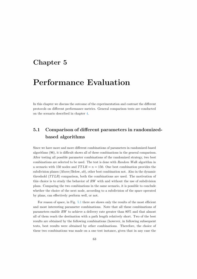
Chapter 5
Performance Evaluation
In this chapter we discuss the outcome of the experimentation and contrast the different
protocols on different performance metrics. General comparison tests are conducted
on the scenario described in chapter 4.
5.1 Comparison of different parameters in randomized-
based algorithms
Since we have more and more different combinations of parameters in randomized-based
algorithms (96), it is difficult shows all of these combinations in the general comparison.
After testing all possible parameter combinations of the randomized strategy, two best
combinations are selected to be used. The test is done with Random Walk algorithm in
a scenario with 150 nodes and TTLR = n = 150. One best combination provides the
subdivision planes (Above/Below, ab), other best combination not. Also in the dynamic
threshold (TTLR) comparison, both the combinations are used. The motivation of
this choice is to study the behavior of RW with and without the use of subdivision
plans. Comparing the two combinations in the same scenario, it is possible to conclude
whether the choice of the next node, according to a subdivision of the space operated
by plans, can effectively perform well, or not.
For reason of space, in Fig. 5.1 there are shows only the results of the most efficient
and most interesting parameter combinations. Note that all these combinations of
parameters enable RW to achieve a delivery rate greater than 80% and that almost
all of them reach the destination with a path length relatively short. Two of the best
results are obtained by the following combinations (however, in following subsequent
tests, best results were obtained by other combinations. Therefore, the choice of
these two combinations was made on a one test instance, given that in any case the
63

64 CHAPTER 5. PERFORMANCE EVALUATION
differences in performance were minimal).
• m = 3, R = Greedy, S = Angle, ab = Y ES
• m = 2, R = Compass, S = Angle, ab = NO
40% 50% 60% 70% 80% 90%
Delivery rate %
m=2,R=1,S=0,ab=0
m=2,R=1,S=1,ab=0
m=2,R=1,S=2,ab=0
m=2,R=1,S=3,ab=0
m=2,R=2,S=0,ab=0
m=2,R=2,S=1,ab=0
m=2,R=2,S=2,ab=0
m=2,R=2,S=3,ab=0
m=2,R=3,S=0,ab=0
m=2,R=3,S=1,ab=0
m=2,R=3,S=2,ab=0
m=2,R=3,S=3,ab=0
m=3,R=1,S=2,ab=1
m=3,R=2,S=2,ab=1
m=3,R=2,S=2,ab=1
m=3,R=2,S=3,ab=1
m=3,R=3,S=1,ab=1
m=3,R=3,S=2,ab=1
m=3,R=3,S=3,ab=1
Random
Walk
- P
ara
mete
rs C
om
bin
ati
ons
(a)
0 1 2 3 4
Path Dilation
m=2,R=1,S=0,ab=0
m=2,R=1,S=1,ab=0
m=2,R=1,S=2,ab=0
m=2,R=1,S=3,ab=0
m=2,R=2,S=0,ab=0
m=2,R=2,S=1,ab=0
m=2,R=2,S=2,ab=0
m=2,R=2,S=3,ab=0
m=2,R=3,S=0,ab=0
m=2,R=3,S=1,ab=0
m=2,R=3,S=2,ab=0
m=2,R=3,S=3,ab=0
m=3,R=1,S=2,ab=1
m=3,R=2,S=2,ab=1
m=3,R=2,S=2,ab=1
m=3,R=2,S=3,ab=1
m=3,R=3,S=1,ab=1
m=3,R=3,S=2,ab=1
m=3,R=3,S=3,ab=1
Random
Walk
- P
ara
mete
rs C
om
bin
ati
ons
(b)
Figure 5.1: Performance of best parameters combinations in Random Walk, considering
the simulation scenario described in 4.1 with 150 nodes. m is the number
of candidate nodes, R indicates which strategy is used to choose candidate
nodes (random, greedy, compass, most forward), S indicates how the chances of
choosing the next node are made (uniform, distance, angle, projected distance)
and ab indicates if consider planes subdivision or not.
In Single Flow scenario, both combinations are used in RW and only the combination
with plane subdivision (ab = Y ES) is used in other random algorithms (GRG, RW-
CFace(1)-RW, RW-CFace(3)). In Multi Flows scenario only the combination with
plane subdivision is used in all the algorithms.
5.2 Standard comparison results
Results of general comparison of all the algorithms of this thesis is shown in Figs. 5.2,
5.3, 5.4 and 5.5, respectively related to 50, 100, 150 and 200 nodes in the graphs. It
it immediately evident, from the result given in those graphics, that deterministic

5.2. STANDARD COMPARISON RESULTS 65
progress-based algorithms (Greedy, Compass, Most Forward and Ellipsoid, in first 4
columns) have the lowest delivery rate, less than 60% in the case of 150 nodes (Fig.
5.4a). This makes clear that cubic networks with side length of 500 units and 150
hosts, are a critical scenario for deterministic progress-based algorithms, because there
is more chance of finding local minima. Instead, as seen in other cases (Figs. 5.2a,
5.3a and 5.5a) delivery rate of the same algorithms tends to increase. About path
dilation, deterministic progress-based can nearly always find the minimum path, thus
obtaining a path dilation value close to 1, as seen in all path dilation histograms. For
this reason this type of algorithms are used in combination with algorithms that offer
a high delivery rate, but a too high traffic.
RW algorithm, obtains better results in delivery rate, but slightly worse results in
path dilation (between 2 and 3). This decline is not very bad, whereas the delivery rate
can exceed a value of 90% in case of 50 nodes, as seen in Fig. 5.2a. As seen, in all four
scenarios the performance of two combinations of parameters in RW are the same, with
a slight increase by the combination m = 3, R = Greedy, S = Angle, ab = Y ES for
n = 200 (Fig. 5.5a). This means that with this scenario configuration the forwarding
strategy with plane subdivision perform well not significantly.
Maintaining a delivery rate almost equal, also GRG offers a shorter path in all four
network sizes, since a Greedy scheme is integrated in this. This can be noticed, for
example, in Fig. 5.4 where RW and GRG delivery rate’s columns are almost at the
same height (Fig. 5.4a), while GRG path dilation’s column is lowest than the column
of RW (m = 3, R = Greedy, S = Angle, ab = Y ES) (Fig. 5.4b), and also the delivery
time is reduced (Fig. 5.4c).
Face-based routing algorithms (Projective Face, CFace(3) and ALSP Face) can
generally achieve better results than the previous ones. As can be seen in Fig. 5.2a,
these have better performance than randomized-based algorithms (about 97% of
delivery in some cases), but when the size network grows, in Figs. 5.3a, 5.4a and
5.5a, a little overcoming of delivery rate can be noted. CFace(3) can be defined as
Projective Face, only choosing two plans that are xy plane and xz plane, and with
the addition of the xz plane. So, since the algorithm have three chances to find the
destination instead of two as Projective Face, the delivery rate is a little higher, with
a little higher path dilation (TTLF is counted 3 times). However, the results of all
these three algorithms, regarding the number of traveled hops, are very bad, with
a path dilation that reaches peaks of 35 times the minimum path length (see Fig.
5.5b). It means that many instances of tests use almost all the set global threshold,
TTL, before the packet reaches the destination. In particular, for CFace(3) and ALSP
Face, when the graph size increase, there is an increase in the number of crossing
edges, which means greater chance for entering into loops, therefore increasing the
probability of having to project to the second and third plane. Face-based strategy is
born to give a guaranteed delivery in two-dimensional graphs, and forcing of these in

66 CHAPTER 5. PERFORMANCE EVALUATION
three-dimensional environments causes a series of long and unnecessary forwards of
packets, since no planarization of graphs is applied.
Greedy-Face-Greedy algorithm is particularly able to find a short routing path and it
is used to reduce the bad effects caused by the above three seen algorithms. Comparing
the difference in performance of ALSP and GFG (that uses ALSP strategy) algorithms,
as can be seen in the results of the path dilation in Figs. 5.2b, 5.3b, 5.4b and 5.5b
(ALSP and GFG histograms), the values of the latter are reduced considerably, reaching
a maximum of 15 times the minimum path length. Moreover, GFG offers better results
compared to ALSP, also with regard to the delivery of the packet.
In comparison of CFace(3) with the two RW-CFace(1)-RW and RW-CFace(3), it is
seen that RW-CFace(1)-RW performs better than CFace(3) in terms of delivery, and
decreases the path dilation. RW-CFace(3) reaches an higher delivery rate (about 98%),
always maintaining a low path dilation, compared to CFace(3) (the small increase in
the path length of RW-CFace(3) is due to the fact that the algorithm does not return
to RW phase, but continues with CFace(3) until the threshold expires).
LAR and RW-LAR algorithms are partial flooding-based. LAR has a relevant
traffic with a nearly guaranteed delivery in case of fewer and closer nodes. In more
large networks, because increasing the number of nodes implies increasing of density,
the path dilation of LAR increases, because the restriction area includes many more
nodes, and the delivery rate decreases. The descent of the delivery rate is due to
the increase of nodes covering around the 3D cube simulation. This increases the
probability that the path from source to destination lies outside the LAR area.
DFS algorithm maintains a guaranteed delivery in a static network. Then, only its
path dilation is analyzed. Since increasing the number of nodes implies increasing the
possibility for long detours being discovered during depth search, the path dilation is
increased; however, to 200 nodes (Fig. 5.5b the value does not exceed 4, reaching a
less traffic than GFG and RW-LAR. Whereas it achieves a delivery rate of 100%, it is
one of the best algorithms, except that it is not a memoryless algorithm (this question
is discussed in the conclusions).

5.2. STANDARD COMPARISON RESULTS 67
Gre
edy
Com
pass
Mos
t Fo
rwar
d
Ellip
soid
RW
(2,
CM
,A,a
b=NO)
RW
(3,
GR,A
,ab=
YES)
Proj
ective
Fac
e
Cfa
ce(3
)
ALS
P Fa
ce
GFG
RW
-CFa
ce(1
)-RW
RW
-CFa
ce(3
)
GRG
LAR
RW
-LAR
DFS
Routing Algorithms
40%
50%
60%
70%
80%
90%
100%
Delivery
Rate
%
(a)
Gre
edy
Com
pass
Mos
t Fo
rwar
d
Ellip
soid
RW
(2,
CM
,A,a
b=NO)
RW
(3,
GR,A
,ab=
YES)
Proj
ective
Fac
e
Cfa
ce(3
)
ALS
P Fa
ce
GFG
RW
-CFa
ce(1
)-RW
RW
-CFa
ce(3
)
GRG
LAR
RW
-LAR
DFS
Routing Algorithms
0
5
10
15
20
25
30
35
40
Path
Dilati
on
(b)
Gre
edy
Com
pass
Mos
t Fo
rwar
d
Ellip
soid
RW
(2,
CM
,A,a
b=NO)
RW
(3,
GR,A
,ab=
YES)
Proj
ective
Fac
e
Cfa
ce(3
)
ALS
P Fa
ce
GFG
RW
-CFa
ce(1
)-RW
RW
-CFa
ce(3
)
GRG
LAR
RW
-LAR
DFS
Routing Algorithms
0
10
20
30
40
50
60
Delivery
Tim
e (
ms)
(c)
Figure 5.2: Delivery rate (a), path dilation (b), and delivery time (c) of all algorithms, in a
graph of 50 nodes, with TTLF = 2N (100), TTLR = N (50) and TTL = 6N
(300)

68 CHAPTER 5. PERFORMANCE EVALUATION
Gre
edy
Com
pass
Mos
t Fo
rwar
d
Ellip
soid
RW
(2,
CM
,A,a
b=NO)
RW
(3,
GR,A
,ab=
YES)
Proj
ective
Fac
e
Cfa
ce(3
)
ALS
P Fa
ce
GFG
RW
-CFa
ce(1
)-RW
RW
-CFa
ce(3
)
GRG
LAR
RW
-LAR
DFS
Routing Algorithms
40%
50%
60%
70%
80%
90%
100%D
elivery
Rate
%
(a)
Gre
edy
Com
pass
Mos
t Fo
rwar
d
Ellip
soid
RW
(2,
CM
,A,a
b=NO)
RW
(3,
GR,A
,ab=
YES)
Proj
ective
Fac
e
Cfa
ce(3
)
ALS
P Fa
ce
GFG
RW
-CFa
ce(1
)-RW
RW
-CFa
ce(3
)
GRG
LAR
RW
-LAR
DFS
Routing Algorithms
0
5
10
15
20
25
30
35
40
Path
Dilati
on
(b)
Gre
edy
Com
pass
Mos
t Fo
rwar
d
Ellip
soid
RW
(2,
CM
,A,a
b=NO)
RW
(3,
GR,A
,ab=
YES)
Proj
ective
Fac
e
Cfa
ce(3
)
ALS
P Fa
ce
GFG
RW
-CFa
ce(1
)-RW
RW
-CFa
ce(3
)
GRG
LAR
RW
-LAR
DFS
Routing Algorithms
0
10
20
30
40
50
60
Delivery
Tim
e (
ms)
(c)
Figure 5.3: Delivery rate (a), path dilation (b) and delivery time (c) of all algorithms, in a
graph of 100 nodes, with TTLF = 2N (200), TTLR = N (100) and TTL = 6N
(600)

5.2. STANDARD COMPARISON RESULTS 69
Gre
edy
Com
pass
Mos
t Fo
rwar
d
Ellip
soid
RW
(2,
CM
,A,a
b=NO)
RW
(3,
GR,A
,ab=
YES)
Proj
ective
Fac
e
Cfa
ce(3
)
ALS
P Fa
ce
GFG
RW
-CFa
ce(1
)-RW
RW
-CFa
ce(3
)
GRG
LAR
RW
-LAR
DFS
Routing Algorithms
40%
50%
60%
70%
80%
90%
100%
Delivery
Rate
%
(a)
Gre
edy
Com
pass
Mos
t Fo
rwar
d
Ellip
soid
RW
(2,
CM
,A,a
b=NO)
RW
(3,
GR,A
,ab=
YES)
Proj
ective
Fac
e
Cfa
ce(3
)
ALS
P Fa
ce
GFG
RW
-CFa
ce(1
)-RW
RW
-CFa
ce(3
)
GRG
LAR
RW
-LAR
DFS
Routing Algorithms
0
5
10
15
20
25
30
35
40
Path
Dilati
on
(b)
Gre
edy
Com
pass
Mos
t Fo
rwar
d
Ellip
soid
RW
(2,
CM
,A,a
b=NO)
RW
(3,
GR,A
,ab=
YES)
Proj
ective
Fac
e
Cfa
ce(3
)
ALS
P Fa
ce
GFG
RW
-CFa
ce(1
)-RW
RW
-CFa
ce(3
)
GRG
LAR
RW
-LAR
DFS
Routing Algorithms
0
10
20
30
40
50
60
Delivery
Tim
e (
ms)
(c)
Figure 5.4: Delivery rate (a), path dilation (b) and delivery time (c) of all algorithms, in a
graph of 150 nodes, with TTLF = 2N (300), TTLR = N (150) and TTL = 6N
(900)
70 CHAPTER 5. PERFORMANCE EVALUATION
Gre
edy
Com
pass
Mos
t Fo
rwar
d
Ellip
soid
RW
(2,
CM
,A,a
b=NO)
RW
(3,
GR,A
,ab=
YES)
Proj
ective
Fac
e
Cfa
ce(3
)
ALS
P Fa
ce
GFG
RW
-CFa
ce(1
)-RW
RW
-CFa
ce(3
)
GRG
LAR
RW
-LAR
DFS
Routing Algorithms
40%
50%
60%
70%
80%
90%
100%D
elivery
Rate
%
(a)
Gre
edy
Com
pass
Mos
t Fo
rwar
d
Ellip
soid
RW
(2,
CM
,A,a
b=NO)
RW
(3,
GR,A
,ab=
YES)
Proj
ective
Fac
e
Cfa
ce(3
)
ALS
P Fa
ce
GFG
RW
-CFa
ce(1
)-RW
RW
-CFa
ce(3
)
GRG
LAR
RW
-LAR
DFS
Routing Algorithms
0
5
10
15
20
25
30
35
40
Path
Dilati
on
(b)
Gre
edy
Com
pass
Mos
t Fo
rwar
d
Ellip
soid
RW
(2,
CM
,A,a
b=NO)
RW
(3,
GR,A
,ab=
YES)
Proj
ective
Fac
e
Cfa
ce(3
)
ALS
P Fa
ce
GFG
RW
-CFa
ce(1
)-RW
RW
-CFa
ce(3
)
GRG
LAR
RW
-LAR
DFS
Routing Algorithms
0
10
20
30
40
50
60
Delivery
Tim
e (
ms)
(c)
Figure 5.5: Delivery rate (a), path dilation (b) and delivery time (c) of all algorithms, in a
graph of 200 nodes, with TTLF = 2N (400), TTLR = N (200) and TTL = 6N
(1200)

5.3. COMPARISON RESULTS WITH DYNAMIC THRESHOLD VALUES 71
5.3 Comparison results with dynamic threshold val-
ues
The aim of this test is to see the effect of the threshold respectively for randomized-
based and face-based algorithms. That is, to see how effective is to increase their
threshold values (TTLR and TTLF ) to increase performance. To get a fair treatment
of the various instances of tests, the TTL value is calculated equal to 2 ∗ TTLR for
random comparison and to 3∗TTLF for face comparison, as in this test are the TTLR
and TTLF thresholds to be dynamic in this test, and not the number of nodes n.
5.3.1 Dynamic TTLR threshold
Figs. 5.6 show the effect of varying the TTLR threshold value on the average delivery
and average path dilation of the two algorithms that use pure randomized strategy,
Random Walk and GRG, with two parameters combinations. Remember that the two
best parameters combination chosen and used on both the algorithms in this test are:
• m = 3, R = Greedy, S = Angle, ab = Y ES
• m = 2, R = Compass, S = Angle, ab = NO
As seen in Fig. 5.6a, the delivery rate is generally stable from a TTLR value of 150.
It means that, in this scenario and this configuration of the network, it is useless to
increase the threshold value up to n, to increase the chance to reach the destination.
Since the little increasing of the delivery rate means more success delivered packets
added to the average path dilation, then there is an increase of the path dilation. The
simulation results also confirm this expectation, with an increase in the path dilation,
as seen in Fig. 5.6b, corresponding to an increase in TTL threshold.
5.3.2 Dynamic TTLF threshold
Figs. 5.7 shows the effect of varying the TTLF threshold value on the average delivery
and average path dilation of the four algorithms that use pure face strategy, Projective
Face, CFace(3), ALSP Face and GFG. Remember that GFG uses ALSP Face algorithm
as recovery phase. The increase in the delivery rate, in Fig. 5.7a, is very significant
for all the algorithms until the threshold value of 300 (2n). Fig. 5.7b shows the
corresponding path dilation, that continues to increase even though the delivery rate
stop increasing noticeably. This indicates that a lot of looping occurs during the
routing process. ALSP Face, CFace(3) and GFG algorithms perform well together in
terms of delivery rate, than other algorithms, but CFace(3) has a path dilation that
grows more compared to the other. GFG algorithm perform well in delivery rate, as

72 CHAPTER 5. PERFORMANCE EVALUATION
75 150 225 300
TTLR threshold
60%
70%
80%
90%
100%
Delivery
Rate
%
RW (3, GR, A, ab=YES)
RW (2, CM, A, ab=NO)
GRG (3, GR, A, ab=YES)
GRG (2, CM ,A , ab=NO)
(a)
75 150 225 300
TTLR threshold
0
1
2
3
4
5
Path
Dilati
on
RW (3, GR, A, ab=YES)
RW (2, CM, A, ab=NO)
GRG (3, GR, A, ab=YES)
GRG (2, CM ,A , ab=NO)
(b)
Figure 5.6: Delivery rate (a) and path dilation (b) of Random Walk and Greedy-Random-
Greedy algorithms, in a graph of 150 nodes, with TTLR = 75, 150, 225, 300,
and a global threshold TTL of 2 ∗ TTLR.

5.3. COMPARISON RESULTS WITH DYNAMIC THRESHOLD VALUES 73
150 300 450 600
TTLF Threshold
60%
70%
80%
90%
100%
Delivery
Rate
%
Projected Face
Cface(3)
ALSP Face
GFG
(a)
150 300 450 600
TTLF Threshold
10
20
30
40
50
Path
Dilati
on
Projected Face
Cface(3)
ALSP Face
GFG
(b)
Figure 5.7: Delivery rate (a) and path dilation (b) of Projected Face, CFace(3), ALSP Face
and GFG algorithms, in a graph of 150 nodes, with TTLF = 150, 300, 450,
600, a global threshold TTL of 3 ∗ TTLF and an ABS value of 100.

74 CHAPTER 5. PERFORMANCE EVALUATION
ALSP Face, and has the least path dilation than other algorithms (the value remains
permanently below 10). Moreover, GFG has a path length that increases much more
slowly than the others one; this means that even for very long threshold values, it can
reach the destination with short path.
5.4 Comparison results with noise traffic
Figs. 5.8, 5.9, 5.10 show the results from Multi Flow simulations. From the test, the
noise traffic has not affected little the performance of almost all algorithms (path
dilation is not shown in this test, since results would be the same as those in Single
Flow simulations). The only decrease in performance can be seen in face-based
algorithms, where the delivery rate decreases much. Following a longer path and
being in competition with multiple streams, with face routing some packets may drop.
CFace(3) has the greatest descent in the case of 40 flows, as seen in Fig. 5.10a. Moreover,
always the face-based algorithms have an high delay to delivering the packet (more
than 1 second), caused by the many queues due to traffic. It is clearly that face-based
algorithms are not suitable to a scenario with multi data streams. Progress-based,
randomized-based and DFS algorithms have not noticeable performance degradation.
The slight decrease in the delivery rate in DFS is due to lack of the neighborhood
information: in tests there have been cases of empty neighbor table, caused by the fact
that the hello messages, in response to the position request messages came later than
the expiry of timerSend (caused by queues), resulting in a packet forwarding with an
empty neighborhood, and then a subsequent failure.
5.5 Comparison results with dynamic min path length
This section shows the results relating to the application of all the routing algorithms
considered in classes of graphs in which the length of the shortest path source-destination
is respectively 1-3, 4-6, 7-9, and >10 hops. These results can be seen in Figs. 5.11,
5.12, 5.13, 5.14. Note that for the first class (1-3 hops), all the algorithms have a
high delivery rate and a small path dilation. This happens because there is very little
chance that in a so few hop distance there are holes (local minima).
When it start to move to longer paths, deterministic progress-based strategies are
the first to degenerate, because, as the destination is more distant, there is a greater
probability to finding holes (localm minima). As seen in Fig. 5.14a, progress-based
algorithms reach about 10% of delivery rate.
RW and GRG algorithms perform well up to 4-6 length of minimum path, but
from this point the delivery rate decreases. This is because the increasing of number of
link to choose from source to destination reduce the probability of choosing the right

5.5. COMPARISON RESULTS WITH DYNAMIC MIN PATH LENGTH 75
Gre
edy
Com
pass
Mos
t Fo
rwar
d
Ellip
soid
RW
(3,
GR,A
,ab=
YES)
Proj
ective
Fac
e
Cfa
ce(3
)
ALS
P Fa
ce
GFG
RW
-CFa
ce(1
)-RW
RW
-CFa
ce(3
)
GRG
LAR
RW
-LAR
DFS
Routing Algorithms
30%
40%
50%
60%
70%
80%
90%
100%D
elivery
Rate
%
(a)
Gre
edy
Com
pass
Mos
t Fo
rwar
d
Ellip
soid
RW
(3,
GR,A
,ab=
YES)
Proj
ective
Fac
e
Cfa
ce(3
)
ALS
P Fa
ce
GFG
RW
-CFa
ce(1
)-RW
RW
-CFa
ce(3
)
GRG
LAR
RW
-LAR
DFS
Routing Algorithms
0
200
400
600
800
1000
1200
1400
1600
Delivery
Tim
e (
ms)
(b)
Figure 5.8: Delivery rate (a) and delivery time (b) of all algorithms, in a graph of 150 nodes
with 5 concurrent data streams.
path. However, the path length of the delivered packet remain short (see Fig. 5.14b,
RW and GRG histogram).
Performance of face-based and hybridized algorithms are also good for high lengths,
due to the fact that they succeed in reach the destination within the TTLF or TTL,
despite the increasing of the distance from source to destination. However, the length
of path performed and delivery time are too high, due to an increase in the number of
crossing links during the travel.
DFS remains delivery time guaranteed. For path lengths >10, path dilation is
slightly greater than 5, which means that also work well for very long distances.

76 CHAPTER 5. PERFORMANCE EVALUATION
Gre
edy
Com
pass
Mos
t Fo
rwar
d
Ellip
soid
RW
(3,
GR,A
,ab=
YES)
Proj
ective
Fac
e
Cfa
ce(3
)
ALS
P Fa
ce
GFG
RW
-CFa
ce(1
)-RW
RW
-CFa
ce(3
)
GRG
LAR
RW
-LAR
DFS
Routing Algorithms
30%
40%
50%
60%
70%
80%
90%
100%
Delivery
Rate
%
(a)
Gre
edy
Com
pass
Mos
t Fo
rwar
d
Ellip
soid
RW
(3,
GR,A
,ab=
YES)
Proj
ective
Fac
e
Cfa
ce(3
)
ALS
P Fa
ce
GFG
RW
-CFa
ce(1
)-RW
RW
-CFa
ce(3
)
GRG
LAR
RW
-LAR
DFS
Routing Algorithms
0
200
400
600
800
1000
1200
1400
1600
Delivery
Tim
e (
ms)
(b)
Figure 5.9: Delivery rate (a) and delivery time (b) of all algorithms, in a graph of 150 nodes
with 20 concurrent data streams.

5.5. COMPARISON RESULTS WITH DYNAMIC MIN PATH LENGTH 77
Gre
edy
Com
pass
Mos
t Fo
rwar
d
Ellip
soid
RW
(3,
GR,A
,ab=
YES)
Proj
ective
Fac
e
Cfa
ce(3
)
ALS
P Fa
ce
GFG
RW
-CFa
ce(1
)-RW
RW
-CFa
ce(3
)
GRG
LAR
RW
-LAR
DFS
Routing Algorithms
30%
40%
50%
60%
70%
80%
90%
100%
Delivery
Rate
%
(a)
Gre
edy
Com
pass
Mos
t Fo
rwar
d
Ellip
soid
RW
(3,
GR,A
,ab=
YES)
Proj
ective
Fac
e
Cfa
ce(3
)
ALS
P Fa
ce
GFG
RW
-CFa
ce(1
)-RW
RW
-CFa
ce(3
)
GRG
LAR
RW
-LAR
DFS
Routing Algorithms
0
200
400
600
800
1000
1200
1400
1600
Delivery
Tim
e (
ms)
(b)
Figure 5.10: Delivery rate (a) and delivery time (b) of all algorithms, in a graph of 150
nodes with 40 concurrent data streams.

78 CHAPTER 5. PERFORMANCE EVALUATION
Gre
edy
Com
pass
Mos
t Fo
rwar
d
Ellip
soid
RW
(3,
GR,A
,ab=
YES)
Proj
ective
Fac
e
Cfa
ce(3
)
ALS
P Fa
ce
GFG
RW
-CFa
ce(1
)-RW
RW
-CFa
ce(3
)
GRG
LAR
RW
-LAR
DFS
Routing Algorithms
0%
10%
20%
30%
40%
50%
60%
70%
80%
90%
100%D
elivery
Rate
%
(a)
Gre
edy
Com
pass
Mos
t Fo
rwar
d
Ellip
soid
RW
(3,
GR,A
,ab=
YES)
Proj
ective
Fac
e
Cfa
ce(3
)
ALS
P Fa
ce
GFG
RW
-CFa
ce(1
)-RW
RW
-CFa
ce(3
)
GRG
LAR
RW
-LAR
DFS
Routing Algorithms
5
10
15
20
25
30
35
Path
Dilati
on
(b)
Gre
edy
Com
pass
Mos
t Fo
rwar
d
Ellip
soid
RW
(3,
GR,A
,ab=
YES)
Proj
ective
Fac
e
Cfa
ce(3
)
ALS
P Fa
ce
GFG
RW
-CFa
ce(1
)-RW
RW
-CFa
ce(3
)
GRG
LAR
RW
-LAR
DFS
Routing Algorithms
0
50
100
150
200
Delivery
Tim
e (
ms)
(c)
Figure 5.11: Delivery rate (a), path dilation (b), and delivery time (c) of all algorithms, in a
graph of 150 nodes with minimum path length of each pair source-destination
of 1, 2 or 3 hops.

5.5. COMPARISON RESULTS WITH DYNAMIC MIN PATH LENGTH 79
Gre
edy
Com
pass
Mos
t Fo
rwar
d
Ellip
soid
RW
(3,
GR,A
,ab=
YES)
Proj
ective
Fac
e
Cfa
ce(3
)
ALS
P Fa
ce
GFG
RW
-CFa
ce(1
)-RW
RW
-CFa
ce(3
)
GRG
LAR
RW
-LAR
DFS
Routing Algorithms
0%
10%
20%
30%
40%
50%
60%
70%
80%
90%
100%
Delivery
Rate
%
(a)
Gre
edy
Com
pass
Mos
t Fo
rwar
d
Ellip
soid
RW
(3,
GR,A
,ab=
YES)
Proj
ective
Fac
e
Cfa
ce(3
)
ALS
P Fa
ce
GFG
RW
-CFa
ce(1
)-RW
RW
-CFa
ce(3
)
GRG
LAR
RW
-LAR
DFS
Routing Algorithms
5
10
15
20
25
30
35
Path
Dilati
on
(b)
Gre
edy
Com
pass
Mos
t Fo
rwar
d
Ellip
soid
RW
(3,
GR,A
,ab=
YES)
Proj
ective
Fac
e
Cfa
ce(3
)
ALS
P Fa
ce
GFG
RW
-CFa
ce(1
)-RW
RW
-CFa
ce(3
)
GRG
LAR
RW
-LAR
DFS
Routing Algorithms
0
50
100
150
200
Delivery
Tim
e (
ms)
(c)
Figure 5.12: Delivery rate (a), path dilation (b), and delivery time (c) of all algorithms, in a
graph of 150 nodes with minimum path length of each pair source-destination
of 4, 5 or 6 hops.

80 CHAPTER 5. PERFORMANCE EVALUATION
Gre
edy
Com
pass
Mos
t Fo
rwar
d
Ellip
soid
RW
(3,
GR,A
,ab=
YES)
Proj
ective
Fac
e
Cfa
ce(3
)
ALS
P Fa
ce
GFG
RW
-CFa
ce(1
)-RW
RW
-CFa
ce(3
)
GRG
LAR
RW
-LAR
DFS
Routing Algorithms
0%
10%
20%
30%
40%
50%
60%
70%
80%
90%
100%D
elivery
Rate
%
(a)
Gre
edy
Com
pass
Mos
t Fo
rwar
d
Ellip
soid
RW
(3,
GR,A
,ab=
YES)
Proj
ective
Fac
e
Cfa
ce(3
)
ALS
P Fa
ce
GFG
RW
-CFa
ce(1
)-RW
RW
-CFa
ce(3
)
GRG
LAR
RW
-LAR
DFS
Routing Algorithms
5
10
15
20
25
30
35
Path
Dilati
on
(b)
Gre
edy
Com
pass
Mos
t Fo
rwar
d
Ellip
soid
RW
(3,
GR,A
,ab=
YES)
Proj
ective
Fac
e
Cfa
ce(3
)
ALS
P Fa
ce
GFG
RW
-CFa
ce(1
)-RW
RW
-CFa
ce(3
)
GRG
LAR
RW
-LAR
DFS
Routing Algorithms
0
50
100
150
200
Delivery
Tim
e (
ms)
(c)
Figure 5.13: Delivery rate (a), path dilation (b), and delivery time (c) of all algorithms, in a
graph of 150 nodes with minimum path length of each pair source-destination
of 7, 8 or 9 hops.

5.5. COMPARISON RESULTS WITH DYNAMIC MIN PATH LENGTH 81
Gre
edy
Com
pass
Mos
t Fo
rwar
d
Ellip
soid
RW
(3,
GR,A
,ab=
YES)
Proj
ective
Fac
e
Cfa
ce(3
)
ALS
P Fa
ce
GFG
RW
-CFa
ce(1
)-RW
RW
-CFa
ce(3
)
GRG
LAR
RW
-LAR
DFS
Routing Algorithms
0%
10%
20%
30%
40%
50%
60%
70%
80%
90%
100%
Delivery
Rate
%
(a)
Gre
edy
Com
pass
Mos
t Fo
rwar
d
Ellip
soid
RW
(3,
GR,A
,ab=
YES)
Proj
ective
Fac
e
Cfa
ce(3
)
ALS
P Fa
ce
GFG
RW
-CFa
ce(1
)-RW
RW
-CFa
ce(3
)
GRG
LAR
RW
-LAR
DFS
Routing Algorithms
5
10
15
20
25
30
35
Path
Dilati
on
(b)
Alg
oritm
o
Gre
edy
Com
pass
Mos
t Fo
rwar
d
Ellip
soid
RW
(3,
GR,A
,ab=
YES)
Proj
ective
Fac
e
Cfa
ce(3
)
ALS
P Fa
ce
GFG
RW
-CFa
ce(1
)-RW
RW
-CFa
ce(3
)
GRG
LAR
RW
-LAR
DFS
Routing Algorithms
0
50
100
150
200
Delivery
Tim
e (
ms)
(c)
Figure 5.14: Delivery rate (a), path dilation (b), and delivery time (c) of all algorithms, in a
graph of 150 nodes with minimum path length of each pair source-destination
greater than 10 hops.
82 CHAPTER 5. PERFORMANCE EVALUATION
5.6 Summarized Results
A taxonomy of described and tested position-based algorithms is given in table 5.1. It
summarizes the main characteristics of these techniques, reporting the results in terms
of performance quality. These characteristics are described as follows (delivery and
path dilation are already defined in 3.1.3).
• Loop Freedom: a data packet can be resent into the network to nodes that
have previously received the same packet. Thus, the packet can circulate around
the network on the same path. In this context, a loop occurs when a path is
repeated several times and an expiration of a threshold is necessary to terminate
the process.
• Path Strategy: algorithms can use either the single path strategy which requires
only a single packet is present in the network at any time, or the multi path
strategy which requires many copies of the same packet are present in the network.
• Forwarding Method: it indicates the forwarding strategy to send packets.
There are four main forwarding strategies: progress-based, randomized-based,
face-based and hybrid-based, that uses combinations of the first three strategies.
• Memory: there are routing protocols which require nodes to maintain informa-
tion about the status of the other nodes. So, these protocols (e.g., DFS ) can
be categorized according to the memory requirements of the nodes. If nodes
need more than the position information of themselves, their neighbors and the
destination (and other information with complexity O(1)), they are considered
to have a memory requirement.
• Scalability: ad hoc networks have varying size. A routing protocol that perform
well also in large size networks is considered scalable. Scalability is not measured in
a particular way and it depends on the outcome of a certain protocol simulation.
In this thesis, scalability is valued based on the path dilation and memory
requirement.
From the table we can see some considerations. Progress-based forwarding algorithms
are highly scalable, but have a low delivery rate. These algorithms are suitable for
dense and uniform networks, where there are not voids (local minima). Furthermore,
these can be used in combination with other algorithms to reduce the path to reach the
destination. Randomized-based forwarding strategy have one of the best performances
in terms of scalability and delivery. It can outperform the progress-based strategy in
sparse networks. Face-based forwarding algorithms have a significant path dilation;
thus, they are not appropriate for dense networks, because there are many crossed
links, and for flow data scenarios. But they perform well in sparse networks, where
there are few nodes and so few crossed links. Partial flooding-based algorithms can be

5.6. SUMMARIZED RESULTS 83
used in small/medium networks, where multi path strategy does not greatly reduces
the performances. Hybrid-based algorithms can perform well in a large range of
network types, since they combine some advantages from base algorithms: delivery
rate is high, path dilation is not high and scalability is high; this depends on the
progress/randomized strategy combined with face-based methods. The only delivery
guaranteed algorithm is DFS, with a low path dilation. It uses memory requirement.
Several improvements can be make to reduce the amount of data memorized in nodes.
Scalability of this forwarding algorithm can be discussed (see conclusion in Cap. 6),
considering the currently available technologies and methodologies to improver the
memory requirement. If a small/medium network is considered, DFS algorithm is one
of the best choices.
Table 5.1: All the algorithms considered in this thesis, with their characteristic and perfor-
mance results.
3D Algorithm Loop Freedom Path Strategy Forw. Method Memory Delivery Rate Path Dil. Scalability
Greedy Yes Single path Prog-based No Low Very Low High
Compass No Single path Prog-based No Low Very Low High
Most Forward Yes Single path Prog-based No Low Very Low High
Ellipsoid Yes Single path Prog-based No Low Very Low High
Random Walk Yes* Single path Rand-based No Medium Low High
Projective Face No Single path Face-based No Medium High Medium
CFace(3) No Single path Face-based No High High Medium
ALSP face No Single path Face-based No High High Medium
GFG No Single path Hybrid-based No High Medium High
RW-CFace(1)-RW No Single path Hybrid-based No High Medium High
RW-CFace(3) No Single path Hybrid-based No High Medium High
GRG Yes Single path Hybrid-based No Medium Medium High
LAR Yes/No** Multiple path Prog-based Yes/No** Medium High Medium
RW-LAR Yes/No** Multiple path Prog-based*** Yes/No** Medium Medium Medium
DFS Yes Single path Prog-based Yes Guaranteed Low Medium****
* Since randomized, there are no repeated cycles.
** LAR and RW-LAR are loop free if the nodes store received packets in its memory to not
retransmit the same, otherwise, a loop occurs and a time-to-live is necessary to drop the
packets.
*** Even if RW is used for the selection of the nodes, it does not make a random choice, since
the packet is sent to all chosen nodes.
**** DFS uses memory to store the past traffic.


Chapter 6
Conclusions and Future
Works
This thesis has deepened, in many ways, the problem of position-based routing applied
on three-dimensional networks. Firstly, the reasons of using an approach based on
the position are discussed, and then the problems and limitations of the algorithms
that use these techniques. Through experimental evaluation we have shown that
almost all the algorithms do not guarantee the delivery of packets, not even using the
planarization models, which guarantee the delivery of networks to two-dimensional
networks. The reason is that, in 2D networks, searching the border of a face is a trivial
one-dimensional search; in 3D networks the search space is two-dimensional, and for
this reason a local (stateless) routing protocol can not ensure to reach the recipient
node.
Deterministic memoryless progress-based strategies can perform well in very dense
networks, with a path length closed to the minimum path one, but not in sparse
networks, due to the problem of local minima. These algorithms, in particular Greedy,
that is loop-free, may be used in combination with other algorithms, as seen, in order
to reduce effectively the number of nodes traveled.
The random component in a forwarding decision offers a better chance to reach
the destination. In this thesis, recovering all algorithms based on randomization, a
unification of all of these into a single algorithm (Random-Walk), with different input
parameters, is be made. With the best combinations of possible parameters, Random
Walk reaches a delivery rate of 80%, with a path length of at most three times the
minimum path length in the considered scenarios. Hybridizing this with Greedy, getting
GRG, can reduce the path length, up to 1.5 times, reaching a slight improvement of
packets delivery.
85

86 CHAPTER 6. CONCLUSIONS AND FUTURE WORKS
Algorithms based on planarization (face-based algorithms) are able to reach very
high values of performance in delivery of packets, whit the cost of a very high path
length. The choice of one of these algorithms hybridized with a progress-based one
(getting GFG) has, in part, raised from the heavy traffic. However, the application of
two-dimensional geometric concepts, as the planarization of a graph, does not seem to
be a very efficient idea applied in three-dimensional environments, as the number of
crosses links is noticeable when the graph is projected, and the followed path is not
always towards the target node as the two-dimensional case, producing unnecessary
several hops and traffic, that generate, in case of multiple streams, many packets
dropping and an high delivery time.
DFS seems to be one of the best algorithms, with the drawback that requires memory
by the nodes. If the network becomes large, the amount of memory may be prohibitive,
but some considerations about it can be made. For example, information about a
packet in nodes’ memory can be deleted after packet’s time-to-live has expired. So,
since the time-to-live and the bandwidth are small, the amount of routing information
stored in each node is small. Furthermore, nowadays many devices are able to acquire a
large amount of memory consuming very little power energy. The memory requirement
is now no longer a problem and this feature can make scalable also not memoryless
algorithms.
This thesis suggests which protocols are most suitable for certain applications and
helps to understand which of them can be enhanced and which ones are not suitable
for the 3D context. Position-based protocols in 3D networks leaves room for further
research and progress, but its advantages for future network design look very promising.
As future works we deem worth pursuing an approach similar in spirit to [8]. In [8],
an efficient geometric routing algorithms is proposed. Authors consider the routing
on hull, that is a 3D analogue to face routing. The proposal of this methodology is
mainly based on the concept of PUTD (Partial Unit Delaunay Triangulation) to define
a “hull”, in which the algorithm is limited to explore. The basic idea foresees that the
packet, as soon as found in a local minimum, covers only the nodes that are in this
hull, i.e., those nodes that have the greatest likelihood and quickness of reaching the
destination node. This context introduces the notion of subspace, where the packet
can travel through its hull. Such a hull is formed by triangles (group of 3 nodes
connected to each other) and edges (two nodes connected to each other), which can be
obtained through methods similar to planarization, using only the neighborhood to 1
hop away. Once PUDT, on the local minimum m in which Greedy algorithm has locked,
is calculated, Depth First Search algorithm is started, to travel the relative subspace’s
hull. If DFS found a node closer to the destination than m, Greedy restarts. Since
DFS is used for routing, this method is delivery guaranteed, and also DFS requires
less memory and power energy, because not all the nodes are considered, but only
those belonging to the relative hull. This may be an interesting starting point, being

87
one of the possible true extensions of face routing in 3D networks. Further studies can
verify its efficiency and costs in various scenario types (multicast, virtual coordinates,
energy efficient scenario, etc.), with an improvement of the technique.
Some improvements of GRG algorithm are proposed in [28]. The proposed technique
is a memoryless greedy-random-greedy strategy with four improvements that try to
increase the performance of Random Walk method.
• Region Limited Random Walk: when the algorithm switch from Greedy to
Random Walk phase in a node c, a sphere of dimension k-hops with center c is
defined. The algorithm operates within this sphere, that is, Random Walk travels
the nodes that are located at most k hop away from c. The k value increases
when a certain threshold of number of traveled hops is exceeded.
• RW on the hull: the search can be limited on the surface (hull) that delimits
the hole in which Greedy stopped. It uses, as above, the concept of PUTD.
• Sparse subgraph: the concept of connected dominating set is used to applying
the algorithm in a restricted set of few major nodes in the network. This
improvement aims to reduce the number of nodes (and hence reduce number of
edges) in dense regions.
• Power of choice for RW : Random Walk does not send the packet to the node
from which the packet came (this improvement is already implemented in this
thesis).
Random Walk, unlike that above, is memoryless and thus it is highly suitable for
MANETs. This line of research can be further analyzed and deepened, since the
randomization is considered a powerful scheme for routing, applicable for real network.


References
[1] N. Aydin M. Ahmad et al. A. Boukerche B. Turgut. “Routing protocols in ad
hoc networks: A survey”. In: Computer Networks 55 (13) (2011), pp. 3032–3080
(cit. on p. 2).
[2] T. Kun A. Maghsoudlou M. St-Hilaire. “A survey on Geographic Routing Pro-
tocols for Mobile Ad hoc Networks”. In: System and Computer Engineering,
Technical Report SCE-11-03 (2011) (cit. on p. 2).
[3] B. Sadler S. Carpin A. Purohit P. Zhang. “Deployment of Swarms of Micro-
Aerial Vehicles: from Theory to Practice”. In: Proceedings of the 2014 IEEE
International Conference on Robotics and Automation (2014) (cit. on p. 7).
[4] A.E. Abdallah, T. Fevens, and J. Opatrny. “Randomized 3D Position-based
Routing Algorithms for Ad-hoc networks”. In: Proceedings of the Third Annual
International Conference on Mobile and Ubiquitous Systems: Networks and
Services (MOBIQUITOUS) (2006), pp. 1–8 (cit. on pp. 36–38, 44, 50).
[5] J. Opatrny A.E Abdallah T. Fevens. “High delivery rate position-based routing
algorithms for 3d ad-hoc networks”. In: Computer Communications 31 (4) (2007),
pp. 807–817 (cit. on pp. 37, 38, 54).
[6] J. Opatrny A.E. Abdallah T. Fevens. “Hybrid Position-based 3D Routing Algo-
rithms with Partial Flooding”. In: Proceedings of the Canadian Conference on
Electrical and Computer Engineering (2006), pp. 1135–1138.
[7] H.T. Kung B. Karp. “GPSR: Greedy Perimeter Stateless Routing for wireless
networks”. In: Proceedings MOBICOM (2000), pp. 243–254 (cit. on p. 40).
[8] J. Wu C. Liu. “Efficient Geometric Routing in Three Dimensional Ad Hoc
Networks”. In: Proceedings of the 28th Conference on Computer Communications
(IEEE INFOCOM 2009) (2009), pp. 2751–2755 (cit. on p. 86).
[9] P. Bhagwat C. Perkins. “Highly dynamic Destination-Sequenced Distance-Vector
routing (DSDV) for mobile computers”. In: Proceedings ACM SIGCOMM Con-
ference (SIGCOMM ’94) (1994), pp. 234–244 (cit. on p. 10).
89

90 REFERENCES
[10] S. R. Das C. Perkins E. Royer. “Ad hoc On-demand Distance Vector (AODV)
routing”. In: Proceedings of the Second IEEE Workshop on Mobile Computing
System and Application (WMCSA) (1999), pp. 90–11 (cit. on p. 11).
[11] D. Malts D. Johnson. “Dynamic Source Routing in Ad-hoc Wireless Networks”.
In: T. Imielinski, H. Korth (Eds.), Mobile Computing, Kluwer Academic Publisher
(1996), pp. 153–181.
[12] H. Singh E. Kranakis and J. Urrutia. “Compass routing on geometric networks”.
In: Proceedings of the 11th Canadian Conference on Computational Geometry
(CCCG’99) (1999), pp. 51–54 (cit. on pp. 25, 28, 38, 42).
[13] Gregory G. Finn. “Routing and addressing problems in large metropolitan-scale
internetworks”. In: Technical Report ISU/RR-87-180, USC Information Sciences
Institute (ISI) (1987) (cit. on p. 25).
[14] J. Opatrny G. Kao T. Fevens. “3D localized position-based routing with nearly
certain delivery in mobile ad-hoc networks”. In: Proceeding of 2nd International
Symposius on Wireless Pervasive Computing (ISWPC’07) (2007) (cit. on pp. xii,
44, 47, 48).
[15] J. Opatrny G. Kao T. Fevens. “Position-based routing on 3D geometric graphs
in mobile ad hoc networks”. In: Proceeding of 17th Canadian Conference on
Computational Geometry (CCCG’05) (2005), pp. 88–91 (cit. on pp. 29, 41, 42).
[16] L. Kleinrock H. Takagi. “Optimal transmission ranges for randomly distributed
packet radio terminals”. In: IEEE Transactions on Communications 32 (3) (1984),
pp. 246–257 (cit. on pp. 25, 28).
[17] M. Vukojevic I. Stojmenovic I. Russell. “Depth First Search and Location Based
Localized Routing and QoS Routing in wireless networks”. In: IEEE International
Conference on Parallel Processing (2000), pp. 173–180 (cit. on pp. 31, 32).
[18] X. Lin I. Stojmenovic. “Loop-free hybrid single-path/flooding routing algorithms
with guaranteed delivery for wireless networks”. In: IEEE Transactions on
Parallel and Distribution Systems 12 (10) (2001), pp. 1023–1032 (cit. on pp. 25,
26, 28).
[19] D. S. J. De Couto D. R. Karger R. Morris J. Li J. Jannotti. “A Scalable Location
Service for geographic ad hoc routing”. In: Proceedings ACM MOBICOM (2000),
pp. 120–130 (cit. on pp. 2, 16–18).
[20] S. Hayat J. Scherer S. Yahyanejad. “An Autonomous Multi-UAV System for
Search and Rescue”. In: Proceedings of the First Workshop on Micro Aerial
Vehicle Networks, Systems, and Applications for Civilian Use (2015), pp. 33–38
(cit. on p. 7).

REFERENCES 91
[21] R. R. Sokal K. R. Gabriel. “A new statistical approach to geographic variation
analysis”. In: Systematic Zoology (Society of Systematic Biologists) 18 (3) (1969),
pp. 259–270 (cit. on p. 40).
[22] K. Sezaki. K. Yamazaki. “The proposal of geographical routing protocols for
location-aware services”. In: Electronics and Communications in Japan 87(4)
(2004) (cit. on p. 28).
[23] D. Giustiniano M. Asapdour K. Anna Hummel. “Micro Aerial Vehicle Networks
in Practice”. In: Proceedings of the First Workshop on Micro Aerial Vehicle
Networks, Systems, and Applications for Civilian Use (2015) (cit. on p. 8).
[24] T. Braun M. Heissenbuttel. “Optimizing Neighbor Table Accuracy of Position-
Based Routing Algorithms”. In: IEEE INFOCOM 2005 (2005) (cit. on pp. 23,
24).
[25] H. Hartenstein M. Mauve J. Widmer. “A survey of position-based routing in
mobile ad-hoc networks”. In: IEEE Network Magazine 15 (6) (2001), pp. 30–39
(cit. on pp. 2, 9, 12).
[26] I. Stojmenovic P. Bose P. Morin. “Routing with guaranteed delivery in ad hoc
wireless networks”. In: Proceedings of the 3rd international workshop on Discrete
algorithms and methods for mobile computing and communications, ACM Press
(1999), pp. 48–55 (cit. on pp. 38, 40).
[27] P. Morin P. Bose. “Online routing in triangulations”. In: Proceedings of the 10th
Annual International Symposium on Algorithms and Computation (ISAAC’99)
(1999), pp. 113–122 (cit. on pp. 35, 38).
[28] R. Wattenhofer R. Flury. “Randomized 3D Geographic Routing”. In: Proceedings
of the 27th Conference on Computer Communications (IEEE INFOCOM 2008)
(2008) (cit. on p. 87).
[29] L. Kleinrock R. Nelson. “The spatial capacity of a slotted ALOHA multihop
packet radio network with capture”. In: IEEE Transactions on Communications
COM-32 (1984), pp. 684–694 (cit. on p. 35).
[30] F.L. Templin B. Bellur R.G. Ogier M.G. Lewis. “Topology broadcast based on
Reverse Path Forwarding (TBRPF)”. In: RFC 3684, IETF Network Working
Group (2002) (cit. on p. 10).
[31] V.Syrotiuk S. Basagni I. Chlamtac. “A distance routing effect algorithm for
mobility (DREAM)”. In: Proceedings of the Fourth Annual ACM/IEEE Interna-
tional Conference on Mobile Computing and Networking (MOBICOM) (1998),
pp. 76–84.

92 REFERENCES
[32] L. Narayanan S. Durocher D. Kirkpatrick. “On Routing with Guaranteed Delivery
in Three-Dimensional Ad Hoc Wireless Networks”. In: Proceedings of ICDCN
’08 (2008), pp. 546–557 (cit. on p. 14).
[33] A. E. Abdallah S. Liu T. Fevens. “Hybrid Position-based Routing Algorithms for
3D Mobile ad Hoc Networks”. In: Proceedings of the 4th International Conference
on Mobile Ad-hoc and Sensor Networks (2008), pp. 177–186.
[34] I. Stojmenovic. “Position-Based Routing in Ad Hoc Networks”. In: IEEE Com-
munications Magazine 40, No. 7 (July 2002), pp. 128–134 (cit. on pp. 2, 9, 12,
16).
[35] P. Jacquet T. Clausen. “Optimized Link State Routing protocol (OLSR)”. In:
RFC 3626, IETF Network Working Group (October 2003) (cit. on p. 10).
[36] B. N. Bennani T. Fevens A. E. Abdallah. “Randomized AB-Face-AB routing
algorithms in mobile ad hoc networks”. In: Proceedings of the 4th international
conference on Ad-Hoc, Mobile, and Wireless Networks (2005) (cit. on p. 35).
[37] L. Narayanan T. Fevens I. T. Haque. “Randomized routing algorithms in mobile
ad hoc networks”. In: Proceeding of the 1st Algorithms for Wireless and Ad-hoc
Networks (A-SWAN) (2004) (cit. on pp. 35, 38).
[38] N. H. Vaidya Y. B. Ko. “Location-Aided Routing (LAR) in mobile ad hoc
networks”. In: ACM/Baltzer Wireless Networks (WINET) 6 (4) (2000), pp. 307–
321 (cit. on p. 53).


![universita' degli studi di padova - [email protected] - Universit](https://static.fdocuments.in/doc/165x107/620619ec8c2f7b1730049ab8/universita-degli-studi-di-padova-emailprotected-universit.jpg)