UNIVERSIDADE FEDERAL DO CEARÁ FACULDADE DE …©.pdf · universidade federal do cearÁ faculdade...

UNIVERSIDADE FEDERAL DO CEARÁFACULDADE DE ECONOMIA, ADMINISTRAÇÃO, ATÚARIA E CONTABILIDADE

PROGRAMA DE PÓS-GRADUAÇÃO EM ECONOMIA - CAEN

DIEGO DE MARIA ANDRÉ

THREE ESSAYS ON APPLIED MICROECONOMETRICS WITH SPATIALEFFECTS

FORTALEZA

2016


THREE ESSAYS ON APPLIED MICROECONOMETRICS WITH SPATIAL EFFECTS

Tese de Doutorado submetida à Coordenaçãodo Programa de Pós-Graduação em Economia– CAEN, da Faculdade de Economia, Adminis-tração, Atúaria e Contabilidade da Universi-dade Federal do Ceará, como requisito parcialpara a obtenção do título de Doutor em Ci-ências Econômicas. Área de concentração:Econometria aplicada.

Prof. Dr. José Raimundo de Araújo CarvalhoJúnior

FORTALEZA

2016

Dados Internacionais de Catalogação na Publicação Universidade Federal do Ceará

Biblioteca UniversitáriaGerada automaticamente pelo módulo Catalog, mediante os dados fornecidos pelo(a) autor(a)

A573t André, Diego de Maria. Three essays on applied microeconometrics with spatial effects / Diego de Maria André. – 2016. 95 f. : il. color.

Tese (doutorado) – Universidade Federal do Ceará, Faculdade de Economia, Administração, Atuária eContabilidade, Programa de Pós-Graduação em Economia, Fortaleza, 2016. Orientação: Prof. Dr. José Raimundo de Araújo Carvalho Júnior.

1. Microeconometria. 2. Econometria espacial. I. Título. CDD 330


THREE ESSAYS ON APPLIED MICROECONOMETRICS WITH SPATIAL EFFECTSTese de Doutorado submetida à Coordenaçãodo Programa de Pós-Graduação em Economia– CAEN, da Faculdade de Economia, Adminis-tração, Atúaria e Contabilidade da Universi-dade Federal do Ceará, como requisito parcialpara a obtenção do título de Doutor em Ci-ências Econômicas. Área de concentração:Econometria aplicada.

Aprovada em: 18 de Maio de 2016.

BANCA EXAMINADORA

Prof. Dr. José Raimundo de Araújo CarvalhoJúnior (Orientador)

Universidade Federal do Ceará (UFC)

Prof. Dr. João Mário Santos de FrançaUniversidade Federal do Ceará (UFC)

Prof. Dr. Emerson Luís Lemos MarinhoUniversidade Federal do Ceará (UFC)

Prof. Dr. Victor Hugo de Oliveira SilvaInstituto de Pesquisa e Estratégia Econômica do

Ceará (IPECE)

Prof. Dr. Cleyber Nascimento de MedeirosInstituto de Pesquisa e Estratégia Econômica do

Ceará (IPECE)

Aos meus pais e à minha esposa.

AGRADECIMENTOS

Nesse momento tão especial da minha vida, não poderia deixar de agradecer aspessoas que de alguma forma contribuiram para que eu alcançasse o meu objetivo. Emprimeiro lugar, agradeço a Deus, por nos dar a oportunidade de vivenciar esse grandemistério que é a vida.

Agradeço aos meus pais, Haroldo e Célia, que através de muito esforço e dedicação,conseguiram me dar educação e me ensinaram a valorizar as pequenas coisas da vida,mostrando-me que só tem valor aquilo que é conseguido com o suor do nosso trabalho. Sehoje sou Doutor em economia, devo isso eles. Obrigado!

A minha esposa, Talita, que durante os nossos quase 9 anos juntos, sempre temme dado apoio, amor e carinho nos momentos díficeis, sempre me incentivando a continuara busca por soluções quando estou quase desistindo. Sem esses incentivos, com certeza,não teria conseguido. Te amo e Obrigado!

Ao professor José Raimundo, com quem tenho aprendido bastante nesses 6 anosem que temos trabalhado juntos (Mestrado e Doutorado), e cujos ensinamentos levareipara a vida toda.

Aos professores João Mário, Emerson Marinho, Victor Hugo e Cleyber Nasci-mento por disponibilizarem seu tempo para participar da banca de avaliação e por suascontribuições ao trabalho.

Aos demais professores do CAEN por suas contribuições à minha formação acadê-mica.

A todos os funcionários do CAEN, em especial ao Cléber e o S. Adelino, que comsuas conversas e brincadeiras ajudam a tornar o CAEN um lugar especial.

Agradeço ainda à todos os colegas do Laboratório de Econometria e Otimização(LECO), não só os atuais (Sylvia, Abel, Luan, Marcelino, Sara) mas a todos os que emalgum momento passaram pelo LECO durante os 6 anos que trabalho lá (Luis Carlos, Yuri,Isadora), pelo convívio e trocas de conhecimento e experiências. Agradeço também a todosos colegas de Mestrado e Doutorado do CAEN.

Por fim, agradeço ao CAEN por disponibilizar sua estrutura para a realização destetrabalho e a CAPES pela bolsa concedida.

A todos, os meus sinceros agradecimentos.

RESUMO

A presente tese é composta por três capítulos, independentes entre si, em microeconometriaaplicada. O primeiro capítulo aplica o instrumental teórico e empírico da econometriaespacial para analisar os determinantes da demanda residencial de água para a cidadede Fortaleza (Brasil). Estimamos três modelos econométricos, que tem como variáveisexplicativas o preço médio/marginal, a diferença, renda, número de homens e mulheresresidentes, número de banheiros, sob diferentes especificações espaciais: O modelo de erroespacial (SEM), o modelo espacial autorregressivo (SAR) e o modelo espacial autorregressivode médias móveis (SARMA), sendo o modelo SARMA o que melhor se ajusta aos dados.Os resultados indicaram que não controlar pelos efeitos espaciais é uma fonte de erro deespecificação, subestimando o efeito de quase todas as variáveis. Algumas vezes, essasdiferenças podem chegar a 24.66% e 13.32% para a elasticidade-preço no modelo de preçomédio e no modelo de McFadden, respectivamente. No segundo capítulo estima-se adisposição a pagar (WTP) pela redução estocástica de primeira ordem no risco de serroubado, para a cidade de Fortaleza (Brasil). Inspirado por Cameron e DeShazo (2013),desenvolveu-se um modelo simples de escolha que aninha o processo de avaliação contingente(CV) entre loterias e estimou-se por máxima verossimilhança paramétrica e pelo modelode regressão geograficamente ponderada (GWR). Para o modelo global, isto é, sem efeitosespaciais, estimou-se uma disposição a pagar média de R$ 23.35 por mês/por residência, eum valor implícito de um roubo estatístico de R$ 11,969 por crime evitado. Para o modelolocal (GWR), implementou-se o protocolo da krigagem para calcular uma superfície dedisposição a pagar. Os resultados sugerem que embora na periferia a disposição a pagarseja menor, à medida que vamos para o centro da cidade existe muita heterogeneidade nadistribuição espacial da disposição a pagar para a redução do risco de roubo. No terceirocapítulo analisou-se como o rendimento acadêmico de alunos universitários é afetado pelosseus colegas de sala, através de um desenho descontínuo. Utilizando dados da UniversidadeFederal do Ceará (UFC), empregamos o modelo de regressão descontínua (RDD) paraestimar a diferença entre entrar na turma do primeiro ou do segundo semestre. Devido àquantidade de cursos disponível na nossa base de dados, classificamos os cursos em quatrocategorias, de acordo com as notas de entrada no vestibular. Então, procedemos com aestimação de um modelo multi-tratamento. Os resultados mostram que os alunos queforam classificados um pouco acima do limite de vagas (turma do primeiro semestre) têmrendimento acadêmico 2% menor (-0.19) do que alunos que tiveram classificação um poucoabaixo desse limite (turma do segundo semestre). Ademais, encontramos não linearidadesnesses efeitos, assim como Sacerdote (2001) e Zimmerman (2003), com intervalos entre 2.5e -0.18.

Palavras-chave: Demanda por água. Efeitos Espaciais. Crime. Avaliação Contingente.Peer Effects. Regressão Descontínua.

ABSTRACT

This Thesis consists of three independent essays on applied microeconometrics. The firstchapter applies theoretical and empirical tools of spatial econometrics to analyze the deter-minants of residential water demand function for the city of Fortaleza (Brazil). We estimatedthree econometric models, which have as explanatory variables the average/marginal price,the difference, income, number of male and female residents and the number of bathrooms,under different spatial specifications: the Spatial Error Model (SEM), the Spatial Auto-regressive model (SAR), and finally, the Spatial Autoregressive Moving Average model(SARMA), which is the model that best fitted the data. Results suggest that not control-ling for spatial effects is a key specification error, underestimating the effect of almostall variables in the model. Sometimes, these differences can be as high as 24.66 % and13.32 % for price elasticity in the Average Price and the McFadden models, respectively.In the second chapter we estimated willingness to pay (WTP) for a first order stochasticreduction on the risk of robbery, for the city of Fortaleza (Brazil). Inspired by Cameronand DeShazo (2013), we develop a simple choice model that nests a process of contingentvaluation (CV) among lotteries and estimate it by both parametric maximum likelihoodand geographically weighted regression (GWR). For the global model (i.e., without spatialeffects), we estimated an average WTP of R$ 23.35 per month/household, and an implicitvalue of a statistical robbery approximately equal to R$ 11,969 per crime avoided. For thelocal model (GWR), we implement a protocol to calculate a surface of WTP using Krigingtechniques. The results suggests that although peripheries present lower willingness to pay,as long as we go inwards there is plenty of heterogeneity on its spatial distribution forrisk reductions. In the third chapter we analyzed how undergraduate students’ academicperformance is affected by theirs classmates, by means of a “discontinuity design”. Withdata from Ceará Federal University (UFC), we employed regression discontinuity design(RDD) to estimate the difference between entering in the first semester class or secondsemester class. Due to the great courses availability, we assign each course into one of fourcategories depending on its admitted students’ results at the entrance exam. Then, weproceed the estimation exercise using a multi-treatment effect model. Results show thatstudents who were ranked just above the cutoff (first semester class) had an academicperformance 2% smaller (-0.19) than students who were ranked just below the cutoff (se-cond semester class). Moreover, we found non-linearities in this effect, as well as Sacerdote(2001) and Zimmerman (2003), with intervals between 0.5 to -0.18.

Keywords: Water demand. Spatial Effects. Crime. Contingent Valuation. Peer Effects.Regression Discontinuity Design.

LIST OF FIGURES

Figure 1.1 – Geographical location of the city of Fortaleza . . . . . . . . . . . . . . 11Figure 3.1 – Survival Function . . . . . . . . . . . . . . . . . . . . . . . . . . . . . . 39Figure 3.2 – First-Order Stochastic Dominance . . . . . . . . . . . . . . . . . . . . . 41Figure 3.3 – Estimated parameters of spatial distribution - Subject Prob. * Income 49Figure 3.4 – Estimated parameters of spatial distribution - Gender . . . . . . . . . . 49Figure 3.5 – Estimated parameters of spatial distribution - Age . . . . . . . . . . . 50Figure 3.6 – Estimated parameters of spatial distribution - Education . . . . . . . . 50Figure 3.7 – Estimated parameters of spatial distribution - Perception of patrolling . 51Figure 3.8 – Estimated parameters of spatial distribution - Victim of robbery . . . . 51Figure 3.9 – Willingness to Pay - Spatial Distribution . . . . . . . . . . . . . . . . . 52Figure 3.10–Willingness to Pay - Kriging Surface . . . . . . . . . . . . . . . . . . . 53Figure 4.1 – Distribution of normalized assignment grade by courses - Medical school

and Law school . . . . . . . . . . . . . . . . . . . . . . . . . . . . . . . 67Figure 4.2 – Distribution of normalized assignment grade by courses - College of

Economics, Management, Actuarial Science and Accounting . . . . . . 68Figure 4.3 – Distribution of normalized assignment grade by courses - College of

Sciences and College of Agricultural Sciences . . . . . . . . . . . . . . . 69Figure 4.4 – Distribution of normalized assignment grade by courses - College of

Humanities . . . . . . . . . . . . . . . . . . . . . . . . . . . . . . . . . 70Figure 4.5 – Distribution of normalized assignment grade by courses . . . . . . . . . 71Figure 4.6 – IRA results as a function of standard assignment grade . . . . . . . . . 76Figure 4.7 – Sensitivity test . . . . . . . . . . . . . . . . . . . . . . . . . . . . . . . 77Figure 4.8 – McCrary test . . . . . . . . . . . . . . . . . . . . . . . . . . . . . . . . 78Figure 4.9 – IRA results as a function of assignment grade . . . . . . . . . . . . . . 80

LIST OF TABLES

Table 2.1 – Descriptive Statistics . . . . . . . . . . . . . . . . . . . . . . . . . . . . 17Table 2.2 – Estimates Average Price, Marginal Price and Mc Fadden, No Spatial

Effects . . . . . . . . . . . . . . . . . . . . . . . . . . . . . . . . . . . . 23Table 2.3 – Estimates Average Price and McFadden, with Spatial Effects . . . . . . 25Table 2.4 – Total Impact on AP and McFadden Models . . . . . . . . . . . . . . . . 25Table 2.5 – Percentual Variation (%) - 100× βT otalSpatial−βNonSpatial

βNonSpatial. . . . . . . . . . 26

Table 3.1 – Variables’ descriptions . . . . . . . . . . . . . . . . . . . . . . . . . . . . 36Table 3.2 – Sample Description - Total . . . . . . . . . . . . . . . . . . . . . . . . . 37Table 3.3 – Sample description - Protesters . . . . . . . . . . . . . . . . . . . . . . . 38Table 3.4 – Sample description - Willing to Pay . . . . . . . . . . . . . . . . . . . . 38Table 3.5 – Willingness to pay frequency distribution . . . . . . . . . . . . . . . . . 38Table 3.6 – Estimates - Parametric Maximum Likelihood . . . . . . . . . . . . . . . 47Table 3.7 – Results of WTP(R$) from the global parametric model . . . . . . . . . 47Table 3.8 – Estimates for the Local Model - GWR -Adaptive bandwidth . . . . . . . 48Table 4.1 – Variables descriptions . . . . . . . . . . . . . . . . . . . . . . . . . . . . 65Table 4.2 – Descriptive statistics . . . . . . . . . . . . . . . . . . . . . . . . . . . . . 65Table 4.3 – Definitions of treatments groups . . . . . . . . . . . . . . . . . . . . . . 72Table 4.4 – SRD estimates for the effect of being in the first semester class on

students’ IRA . . . . . . . . . . . . . . . . . . . . . . . . . . . . . . . . 75Table 4.5 – Effects of policies in some studies . . . . . . . . . . . . . . . . . . . . . . 76Table 4.6 – Covariates balanced test . . . . . . . . . . . . . . . . . . . . . . . . . . . 78Table 4.7 – SRD estimates for the effect of being in the first semester class on

students’ IRA — Multi-treatment . . . . . . . . . . . . . . . . . . . . . 79Table 4.8 – Incremental and comparison with the control effects . . . . . . . . . . . 81Table 4.9 – SRD estimates for the effect of being in the first semester class on

students’ IRA — Classified by areas of knowledge . . . . . . . . . . . . 87Table 4.10–SRD estimates for the effect of being in the first semester class on

students’ IRA — Divided by semesters . . . . . . . . . . . . . . . . . . 88Table 4.11–SRD estimates for the effect of being in the first semester class on

students’ IRA — Multi-treatment - 15% . . . . . . . . . . . . . . . . . . 89

CONTENTS

1 GENERAL INTRODUCTION . . . . . . . . . . . . . . . . . . . . . . 11

2 SPATIAL DETERMINANTS OF URBAN RESIDENTIAL WATERDEMAND IN FORTALEZA, BRAZIL . . . . . . . . . . . . . . . . . 14

2.1 Introduction . . . . . . . . . . . . . . . . . . . . . . . . . . . . . . . . . 142.2 Water Micro Demand Estimation with Spatial Effects . . . . . . . . 152.3 Data Set . . . . . . . . . . . . . . . . . . . . . . . . . . . . . . . . . . . 162.3.1 The Sample . . . . . . . . . . . . . . . . . . . . . . . . . . . . . . . . . . 162.3.2 Spatial Exploratory Data Analysis . . . . . . . . . . . . . . . . . . . . . . 172.4 Econometric Model . . . . . . . . . . . . . . . . . . . . . . . . . . . . 182.4.1 Non-Spatial Specification . . . . . . . . . . . . . . . . . . . . . . . . . . . 182.4.2 Spatial Specification . . . . . . . . . . . . . . . . . . . . . . . . . . . . . 202.4.3 Why Spatial Effects in Water Demand? . . . . . . . . . . . . . . . . . . . 212.5 Results . . . . . . . . . . . . . . . . . . . . . . . . . . . . . . . . . . . . 222.5.1 Non-Spatial Specification . . . . . . . . . . . . . . . . . . . . . . . . . . . 222.5.2 Spatial Specification . . . . . . . . . . . . . . . . . . . . . . . . . . . . . 242.6 Final Considerations . . . . . . . . . . . . . . . . . . . . . . . . . . . . 26

References . . . . . . . . . . . . . . . . . . . . . . . . . . . . . . . . 28

3 SPATIALWILLINGNESS TO PAY FOR A FIRST-ORDER STOCHAS-TIC REDUCTION ON THE RISK OF ROBBERY . . . . . . . . . . 31

3.1 Introduction . . . . . . . . . . . . . . . . . . . . . . . . . . . . . . . . . 313.2 Data Set . . . . . . . . . . . . . . . . . . . . . . . . . . . . . . . . . . . 353.3 Econometric Model . . . . . . . . . . . . . . . . . . . . . . . . . . . . 393.4 A “Local” Econometric Model . . . . . . . . . . . . . . . . . . . . . . 443.5 Results . . . . . . . . . . . . . . . . . . . . . . . . . . . . . . . . . . . . 463.5.1 Results from the Global Model . . . . . . . . . . . . . . . . . . . . . . . . 463.5.2 Results from the Local Model . . . . . . . . . . . . . . . . . . . . . . . . 483.6 Final Considerations . . . . . . . . . . . . . . . . . . . . . . . . . . . . 53

References . . . . . . . . . . . . . . . . . . . . . . . . . . . . . . . . 55

4 PEER EFFECTS AND ACADEMIC PERFORMANCE IN HIGHEREDUCATION - A REGRESSION DISCONTINUITY DESIGN AP-PROACH . . . . . . . . . . . . . . . . . . . . . . . . . . . . . . . . . 57

4.1 Introduction . . . . . . . . . . . . . . . . . . . . . . . . . . . . . . . . . 57

4.2 Brief empirical literature review . . . . . . . . . . . . . . . . . . . . . 594.2.1 Peer effects . . . . . . . . . . . . . . . . . . . . . . . . . . . . . . . . . . 594.2.2 The use of regression discontinuity design . . . . . . . . . . . . . . . . . . 604.3 The entrance process in Brazilian universities . . . . . . . . . . . . . 624.4 Data . . . . . . . . . . . . . . . . . . . . . . . . . . . . . . . . . . . . . 634.5 Empirical strategy . . . . . . . . . . . . . . . . . . . . . . . . . . . . . 724.6 Results . . . . . . . . . . . . . . . . . . . . . . . . . . . . . . . . . . . . 754.7 Final Considerations . . . . . . . . . . . . . . . . . . . . . . . . . . . . 81

References . . . . . . . . . . . . . . . . . . . . . . . . . . . . . . . . 83

1 GENERAL INTRODUCTION

This Thesis is a collection of three independent essays on microeconometrics usingdata from the city of Fortaleza (Brazil). In the first chapter, I examine the determinantsof urban residential water demand. The second chapter studies willingness to pay for areduction on the risk of robbery. The third chapter studies how “peer effects” determinesacademic performance in high education.

Fortaleza is the state capital of Ceará. Located in northeastern Brazil, a dry climateregion, the city has a population of about to 2.5 million and it is the fifth largest city inBrazil with an area of 313 square kilometers, boasting one of the highest demographicdensities in the country (8,001 per km2). Fortaleza’s economy is mainly based on trade,service, and tourism and its gross domestic product is the largest in northeastern Brazil.For being a large urban center, Fortaleza has many problems and criminality is one ofthese. The city is ranked as number one in intentional lethal violent crimes against lifein Brazil and one of the most violent city in the world, which creates a great sense ofinsecurity among the population. In educational sector, Fortaleza hosted one of the bestuniversity in Brazil, besides many others privates universities, which attracts studentsfrom several cities of the region. In this sense, this thesis analyze three important aspectsof the city of Fortaleza: The Water scarcity, the criminality and the higher education.

Figure 1.1 – Geographical location of the city of Fortaleza

12

The first chapter is “Spatial determinants of urban residential water demand inFortaleza, Brazil”. This essay is a enhanced version of my dissertation, and was publishedwith Professor José Raimundo Carvalho in Water Resources Management1. In this essay weestimated a residential water demand function for the city of Fortaleza, Brazil, consideringthe potential impact of including spatial effects in the model. The empirical evidence is aunique micro-data set obtained through a household water consumption survey carried outin 2007. We estimated three econometric models, which have as explanatory variables theaverage/marginal price, the difference, income, number of male and female residents andthe number of bathrooms, under different spatial specifications: the Spatial Error Model(SEM), the Spatial Autoregressive model (SAR), and finally, the Spatial AutoregressiveMoving Average model (SARMA). Results suggest that the SARMA model is the “best”as shown by a series of tests. Such results contradict conclusions drawn by Chang etal. (2010), House-Peters et al. (2010), and Ramachandran and Johnston (2011). Thismeans, among other things, that not controlling for spatial effects is a key specificationerror, underestimating the effect of almost all variables in the model. Sometimes, thesedifferences can be as high as 24.66 % and 13.32 % for price elasticity in the Average Priceand the McFadden models, respectively.

The second chapter is “Spatial willingness to pay for a first order stochastic reductionon the risk of robbery”2. In this essay we estimated willingness to pay (WTP) for afirst order stochastic reduction on the risk of crimes for residents of a large and denseurban center. Inspired by Cameron and DeShazo (2013), we develop a simple structuralchoice model that nests a process of contingent valuation (CV) among lotteries andestimate it by both parametric maximum likelihood and geographically weighted regression(GWR). Our empirical support is a unique and rich micro data set about victimization inFortaleza, CE (Brazil). For the global model (i.e., without spatial effects), we estimatedan average WTP of R$ 23.35 per month/household, and an implicit value of a statisticalrobbery approximately equal to R$ 11,969 per crime avoided. By means of geographicallyweighted regression (GWR), we find that variables Sex, Age and Education present areasonable amount of spatial heterogeneity and, as expected, follow the very inertial city’ssocioeconomic spatial distribution profile. We implement as well a protocol to calculate asurface of WTP using Kriging techniques. Income, age, and crime spatial distributions haveimportant effects on the surface of WTP. Although peripheries present lower willingnessto pay, as long as we go inwards there is plenty of heterogeneity on its spatial distributionfor risk reductions. Our results supports a theory of crime with an active role for victim(costly) precautions.1 Spatial Determinants of Urban Residential Water Demand in Fortaleza, Brazil. Water Resources

Management , v. 28, p. 2401-2414, 2014.2 This essays was presented at the 42nd economics national meeting - ANPEC 2014, at the VII CAEN-

EPGE Public Policy and Economic Growth meeting (2015) and accepted for presentation at theSpatial Econometrics Association Annual meeting - IX world conference SEA 2015 (Miami, USA).

13

The third chapter is “peer effects and academic performance in higher education - aregression discontinuity design approach”. We estimated peer effects in undergraduatestudents’ academic performance at a Brazilian university. Our empirical evidence comesfrom a micro data set containing information of 1550 undergraduate students enrolled in27 courses at the Federal University of Ceará. In light of this great courses availability, weassign each course into one of four categories depending on its admited students’ resultsat the entrance exam. Then, we proceed the estimation exercise using a multi-treatmenteffect model. In this fashion, using IRA as a measure of academic performance, we obtaina negative effect (-0.19) for being in a first semester class, which means a 2% smallerIRA for firt semester students, vis-a-vis members of second semester classes. Moreover,we found non-linearities in this effect, since, for example, it ranges between 0.5 to -0.18.This results are in accordance with Sacerdote (2001) and Zimmerman (2003), also findingnon-linearities in “peer effects”.

2 SPATIAL DETERMINANTS OF URBANRESIDENTIAL WATER DEMAND INFORTALEZA, BRAZIL

2.1 INTRODUCTIONThe literature on residential water demand estimation has grown considerably, indicat-

ing the main variables that affect water consumption and the estimation techniques to beemployed. However, that line of research has not been yet capable of fully exploring howspatial effects might influence water demand. Franczyk and Chang (2009) point out that “water consumption standards cannot be explained by economic and population growthonly, but also through biophysical and socioeconomic factors that usually have spatialdependence”. Following the same line, House-Peters, Pratt and Chang (2010) suggestthat “residential water consumption is not affected by climate, socioeconomic and physicalvariables only. It is also affected by geographical location and its interaction with nearbyregions.”

Therefore, incorporating spatial effects into the analysis of residential water demandcould provide a wider and more accurate explanation on its consumption variations. Paperslike Chang, Parandvash and Shandas (2010), Wentz and Gober (2007), Franczyk andChang (2009), House-Peters, Pratt and Chang (2010), Ramachandran and Johnston (2011)have recently included spatial effects in their studies, increasing the significance of theirmodels when compared to other models that do not consider such effects. Based on thatseries of papers, we believe that our endeavor has its own merits. Firstly, because estimateson water micro-demand models with spatial effects are quite new in international literatureand absent in the national research. Secondly, because by aggregating new methodologicalprocedures we can better understand the factors that affect residential water demand.

Therefore, this paper aims at analyzing water demand using spatial econometrictechniques in an exploratory way. For this, we have at our disposal information froma study field in the city of Fortaleza, Brazil (The state capital of Ceará, located inNortheastern Brazil - WGS84 coordinates 3043′6′′

South and 38032′34′′West). The city

has a population of about to 2.5 million and it is the fifth largest city in Brazil with anarea of 313 square kilometers, boasting one of the highest demographic densities in thecountry (8,001 per km2).

From a series of test procedures and econometric exercises, we can confirm the im-portance of considering spatial effects, since the exclusion of those effects underestimatethe impact that income and the number of bathrooms per residence can have over water

15

demand. More importantly, it underestimate considerably the impact of average andmarginal prices on water demand. Although our results are of an exploratory nature,we believe they will enable us to better understand how space matters for water-microdemand estimation.

Besides this introduction and a section discussing final considerations, this paperhas four more sections. Section 2 offers a brief literature review on residential watermicro-demand estimation. Section 3 introduces the database used and the results of anexploratory spatial data analysis. Section 4 sets up the demand function to be estimatedwith a non-linear tax structure. We also introduce the econometric models used in thispaper together with the tests used for (mis)specification analysis. Finally, Section 5 showsthe results and Section 6 draws some final considerations.

2.2 WATER MICRO DEMAND ESTIMATION WITH SPATIALEFFECTS

To understand the way in which charging water use affects its consumption, it isnecessary to know the factors that determine water demand. Since Gottlieb (1963) andHowe and Linaweaver (1967), several researchers in many countries have carried outstudies to estimate a residential water demand function for their particular regions inorder to provide technical work as a support to implement policies aimed at controllingand promoting its rational use and preservation.

Agthe, Billings and Dobra (1986) for Tucson, Arizona (USA), Rietveld, Rouwendal andZwart (2000) in Indonesia, Polycarpou and Zachariadis (2013) in Cyprus, and Miyawaki,Omori and Hibiki (2013) for the cities of Tokyo and Chiba, are just some representativeexamples. In Brazil, literature on residential water demand estimation is still new. Oneof the first papers that approached this issue was written by Andrade et al. (1995). Forthe city of Piracicaba, São Paulo, Mattos (1998) and Melo and Neto (2007) estimated thefunction of residential water demand for Northeastern Brazil.

Although very heterogenous in terms of methodologies and scopes, all studies brieflycited above share an important shortcoming: they do not consider spatial effects in waterdemand estimation. Aware of this problem, some authors recently started to includespatial effect in their analysis, seeking to explain the spatial association pattern forwater consumption. Wentz and Gober (2007) used GWR model (Geographic WeightedRegression) in a study for Phoenix, USA, in order to verify if there was any additionalspatial effect contribution to the results obtained through the OLS model (Ordinary LeastSquare). The authors verified through the GWR model that the importance of spatialeffects reduces to two the variables that determine water demand. The variables areresidence size and the existence or not of a swimming pool in the property.

16

In the state of Oregon (USA), Franczyk and Chang (2009) realized that water demandwas not just related to population and economic growth, but also to other biophysicaland socioeconomic factors that in general present spatial dependence. The authorsused the spatial error model (SEM), besides the OLS model in order to include spatialautocorrelation effects in the study. They applied Moran-I statistics and showed thatthere is spatial dependence on errors.

In the city of Portland (Oregon, USA) Chang, Parandvash and Shandas (2010) identifieda spatial association pattern for water demand. They verified that the areas where waterconsumption was higher coincided with the areas in which average home sizes were largerand both the building density and property age averages were low. House-Peters, Prattand Chang (2010) carried out a study for the city of Hillsboro (Oregon, USA) analyzingclimate effects on water demand. Using spatial analysis techniques, the authors foundthat although water demand in that area was not sensitive to dry conditions at all, somespecific areas presented higher water consumption levels under such conditions.

Ramachandran and Johnston (2011) studied how the spatial effect influenced residentialwater demand for external use in the city of Ipswich (Massachusetts, USA) while a restricteduse of water policy was being implemented. They argued that decisions on house landscapes,and therefore, the use of water in order to maintain these landscapes would depend oneconomic factors such as if the landscape affects the house selling price or social factorssuch as imitation reasons, as people tend to copy the landscaping and vegetation used ingardens of nearby residences.

2.3 DATA SET

2.3.1 The Sample

The database contains information from a scientific project carried out by a group ofresearchers from UECE and UFC (Ceará State University and Ceará Federal University)requested by CAGECE (Ceará Water and Sewage Company). It collected more than 3,000questionnaires containing information on socioeconomic and physical characteristics fromdifferent households in Fortaleza. After deletion of missing observations, we end up with2,891 usable observations, as shown in Table 2.1.

The data introduced shows that residential water consumption in February 2007 forthe city of Fortaleza was 16.41 m3, on average. The median of 14 m3 indicates that half ofresidences in Fortaleza are either in CAGECE’s first or second consumption block ([0 m3,10 m3] or (10 m3, 15 m3]). This might not be good for CAGECE if the tax structure ispoorly designed. As for the socioeconomic characteristics, on average, each household has2.09 and 1.76 male and female residents respectively. Families have an average monthlyincome of 2.43, which indicates that they spread out between two income classes: class 2

17

Table 2.1 – Descriptive StatisticsMean Std. Dev. Min Median Max

Water Consumption (m3) 16.41 9.71 2.00 14.00 60.00Effective Price (R$) 24.49 21.44 9.80 16.04 159.35Average Price (R$) 1.45 0.56 0.98 1.25 4.90Marginal Price (R$) 1.61 1.02 0.10 1.56 4.95Difference (R$) 9.46 18.68 -8.71 5.80 137.65Family Income (class) 2.43 1.04 1.00 2.00 5.00Type of Property (class) 2.69 0.55 1.00 3.00 4.00Male Residents (number) 2.09 1.16 0.00 2.00 8.00Female Residents (number) 1.76 1.12 0.00 2.00 8.00Bathrooms (number) 1.55 0.86 0.00 1.00 8.00Gardens (dummy) 0.24 0.43 0.00 0.00 1.00Source: Elaborated by the Authors

(whose people earn from one minimum wage (R$ 350.00 or US$ 219.45 - Purchase ParityPower) up to 2 minimum wages), and class 3(those earning from 2 to 5 minimum wages).

With regards to the physical characteristics of households, the residences have, onaverage, 1.55 bathrooms and 24% of them have a garden. The average type of property is2.69, which allows us to classify residences between the medium and regular categoriesaccording to CAGECE’s standards. In terms of pricing, CAGECE applies an increasingtariff system through consumption blocks: [0, 10], (10, 15], (15, 20], (20, 50] and (50,∞).The rates, in 2007, for each block were: R$ 9.80 (Fixed fee), 1.56 R$/m3, 1.65 R$/m3,2.80 R$/m3 and 4.95 R$/m3, respectively. In next section we shall introduce a spatialexploratory analysis applied to our data set.

2.3.2 Spatial Exploratory Data Analysis

In order to check the hypothesis that spatial effect plays an important role to explainresidential water demand, we will verify if water consumption presents any spatial associa-tion pattern at all. Therefore, we stick to the literature and use the Moran-I statistic totest for global spatial association and the local Moran-I statistic to test for local spatialassociation, besides the significances and clusters maps (see, Anselin (1995)).

Moran-I statistics for five well know weighting matrices (distance, 5, 10, 15 and 20nearest neighborhood) were calculated. All figures for the Moran I statistic belong to theinterval (0.0, 0.15). These values exceed their statistical averages but they are close to zero,which apparently indicates no spatial autocorrelation in water consumption. However,although these values are close to zero, they are statistically different from zero, once thepseudo-p-value is extremely low (in fact it is undistinguishable from zero). That is anindication that we cannot reject the hypothesis of lack of positive spatial autocorrelation,even if in a reduced magnitude and for any common weighting matrix. These first resultsprompt us to carry on.

Not always the global pattern of spatial association reflects the local pattern of spatialassociation, though. In this sense, LISA indexes (Local Indicator Spatial Association)

18

are used to overcome this obstacle and capture local patterns of linear association. Themost well known LISA statistic, the local Moran-I, is derived from a global indicatorof autocorrelation that decomposes the local contribution of each observation into fourcategories.

The results of dispersion diagram show that there is a tendency to a positive autocor-relation with the observations distributed in the first and third quadrants for all weightingmatrices, however with a lower value (0.0487) for the distance weighting matrix1.

As for the significance and dispersion maps, they all give similar results for all weightingmatrices: there is a high concentration of water consumption at the top center in the cityof Fortaleza that covers the downtown area and the richest neighborhoods in the city,as well as low consumption clusters in suburban areas2. Hence, such exploratory spatialanalysis confirmed our idea that not only there are global and local spatial autocorrelationpatterns in our sample but also that such spatial autocorrelation might be important.Next section deals with the demand function models specifications and estimations.

2.4 ECONOMETRIC MODEL

2.4.1 Non-Spatial Specification

It is well known that in a setup with non linear prices, the consumer’s budget restrictionwill be non linear as well. In such cases, the solution to the optimization problem faced bya consumer, i.e. maximization of utility given (non-linear) budget constraint, will giveus the water demand as a function of prices and income, according to Moffitt (1986).However, the residential water demand is not a function of water price and consumersincome only.

We need to add other variables, which are important to explain residential waterdemand. Although there is no consensus over the “best” econometric specification formodeling household water demand, we stick to two of the most prominent ones (see,Arbués, García-Valiñas and Espiñeira (2003), Olmstead, Hanemann and Stavins (2007)and Worthington and Hoffman (2008)):

ln (QCi) = β1+β2ln(Pavgi)+β3Inci+β4Malei+β5Femalei+β6Bathi+β7Gardeni+εiln (QCi) = β1 + β2ln(Pmgi) + β3Diffi + β4Inci + β5Malei + β6Femalei + β7Bathi +

β8Gardeni + εi

where,

• QC = Amount of consumed water in February 2007 in m3

• Pavg = Average price in February 20071 Moran-I statistics and all dispersion diagrams can be obtained from the authors upon request.2 Both maps can be obtained from the authors upon request. A possible explanation for the configuration

of such clusters is that the income distribution in the city of Fortaleza is very unequal.

19

• Pmg = Marginal price in February 2007

• Diff = Difference variable3

• Inc = Family Income

• Male = Number of male residents in the household

• Female = Number of female residents in the household

• Bath = Number of bathrooms in the household

• Garden = Dummy for the presence of a garden in the household

• ε = Error term

We decided to start our modeling4 exercise with both the average price and marginalprice coupled with the difference variable specifications based on the following premises.Firstly, the average price versus marginal price (with difference) continues to be an openissue, yet to be settled. Hence, from a methodological point of view it is good practice torely on statistical methodology and not on any ad hoc personal choice of specification exante the modeling exercise.

Secondly, we agree with Saleth and Dinar (2001) when these authors claim that theaverage price versus marginal price issue has not been casted in a correct way whenstressing the question of the lack of perfect information on the water tariff structure or theinexpressive value of water bill compared to household total income. Rather, Saleth andDinar (2001) argue quite convincingly that the price perception debate is not as much of acontroversy on the price specification itself as it is with regards to the relative relevanceof the positive [Pavg] versus normative [Pmg and Diff ] approach to consumer behaviorunder block rate pricing.

Although we may end up choosing the “best” specification, the ... comparison ofdemand functions under these prices can be used to at least show the effects of the changein price levels due to a shift in the price perception. Therefore, the issue on average priceversus marginal price has important behavioral implications beyond the simply traditionaleconometric specification debate, resulting in an almost necessary topic to deal with byestimating both specifications.3 The difference between the bill that would result if each m3 of water consumed was priced by the

marginal price and the actual bill. For increasing block tariffs, the difference is negative for householdslocated on the first block, meaning that their water consumption receives subsidies. See, among others,Nordin (1976)

4 Note that specifications like equations 2.4.1 and 2.4.1 are by no means the only ones. For example,there is growing interest in modeling water demand as composed of two parts; a fixed and a residualcomponent, seeking to capture consumption niches that are non-responsive to pricing (see, Dharmaratnaand Harris (2012)).

20

The choice of socioeconomic variables and the physical characteristics of residencesagree with the main studies carried out on water demand estimation, very well summarizedin Arbués, García-Valiñas and Espiñeira (2003). We expect that family income, numberof male residents and number of female residents in the household, as well as the numberof bathrooms shall exert a positive effect on water demand, since an increase in thesevariables will increase water demand. As for the independent variable presence of garden,we also expect a positive value; however this variable will play an important role whendiscussing spatial effects. Finally, with regards to average, marginal and difference price,it is expected that water reacts as a normal good.

It is known that the estimation of a demand function in a non linear tax context creates,a priori, a problem of endogeneity. We are aware of the potential deleterious impacts ofendogeneity in our estimates (especially on the average price specification) as well as ofauthors that find no significant difference between simple least square estimations andinstrumental variable approaches such the one carried out by Jones and Morris (1984).However, we do control for endogeneity issues, although in a rather traditional way, byestimating the marginal price model through a methodology developed by McFadden,Puig and Kirschner (1977).

Before we proceed to discuss spatial specification issues, it is important to stress thefact that even though Fortaleza is a city located in a developing country, its urban watermarket is very similar to those of cities located in developed countries. Besides being alarge and dense urban center, it has been served by the same water company since 1970,and its customers are used to their tariff system. Also, the market presents an index ofhydrometration above 98%. However, when we move away from the coast, towards innercities in the state of Ceara, the water demand and supply conditions can change quicklyand drastically. On such settings, our model could be a considerable specification error5.

2.4.2 Spatial Specification

To verify if the inclusion of spatial effects affect residential water demand, we usedthree models (see, Anselin (1988)): SEM (Spatial Error Model), which is used when webelieve that spatial dependence is caused by autocorrelation in error terms; mixed SAR(Spatial Autoregressive), that aggregates explicative variables and it is used when thespatial dependence is contained in the dependent variable and finally, the SARMA model(Spatial Autoregressive and Moving Average), that is used when we believe that spatialdependence is contained both in error terms and in the dependent variable. The SARMAmodel is represented by:5 We would like to thank a referee for pointing out that to us.

21

Y = ρW1Y +Xβ + ε (2.1)

ε = λW2ε+ u (2.2)

Y is an n× 1 vector that contains observations on water demand in logarithms. X is ann×m vector of explicative variables, the same used in previous models, and β is an m× 1parameter vector to be estimated, where m is the number of independent variables andn, the sample size. W1 and W2 are the spatial weighting matrixes, u is the random errorterm in standard normal distribution with mean equal zero and a constant variance, andλ is the autoregressive parameter associated to error term. Finally, ρ is the autoregressiveparameter associated to the lagged dependent variable.

In order to help us decide which of the three specifications capture in a more accurateway the spatial effect over residential water demand, we applied Lagrange multiplierstests, both for lag (LMρ) and for spatial error (LMλ), as well as their robust Lagrangemultipliers (RLM) versions. To detect the correct functional form, Florax, Folmer andRey (2003) suggest the use of the "hybrid identification" strategy, using both the classicaland robust tests for spatial autocorrelation.

2.4.3 Why Spatial Effects in Water Demand?

As logical as SARMA model might appear, it subsumes a host of possible theoretical or,according to econometric parlance, "structural", explanations for its channels of causation.However, establishing clear cut causal linkages for spatial models is not an easy task. Infact, according to Corrado and Fingleton (2012), literature on spatial statistics, as wellas spatial econometrics, appear to be dominated by data-analytic considerations onlyduring the model specification phase, to the detriment of causal modeling. However,data-driven protocols are indispensable approaches to perform, especially during theexploratory analysis of statistical and econometric models. A unique reliance on data-analytic considerations trades off against a better understanding of the important behavioraland policy implications of the model. Consequently, a more equilibrated modeling strategyhas to be chosen and this requires a justification on how spatial effects might be importantfor water demand estimation.

The justification for the use of the SARMA model comes from the belief that the spatialeffect might work through both the error terms and/or lags of the dependent variable.Such factors would be the climate-related, biophysical, socioeconomic and geographical, aswell as the infrastructure of the water distribution system. Two theoretical justificationsfor spatial effects that have gained wider acceptance are: i) imitation of consumption inneighboring residences, and ii) water supply network dependencies.

Some authors such as Ramachandran and Johnston (2011) believe that there is imitationof water consumption in neighboring residences, especially in gardening activities, due

22

to the attempt to imitate the shape and type of plants used by neighbors. Althougha seminal idea, their papers fall short after computing descriptive spatial dependenceindexes. Others, like Wentz and Gober (2007) and Janmaat (2013) found similar effects.Janmaat (2013) calls that an emulation effect in water use behavior after modeling waterdemand for the city of Okanagan, Canada, through a geographically weighted regression.Observe, however, that he is very careful to imply a more elaborated causal link beyondasserting that I do not have an explicit theory on how neighbors influence each other ...beyond neighbors noticing each other’s water use. Anyway, we conjecture that imitationor emulation is a possible effect that incorporate (positive) water consumption spatialdependence.

Another possible justification for spatial effects comes from the infrastructure ofwater distribution network systems. A network may create a negative consumptionautocorrelation, once the pressure over the distribution system causes a given residentialconsumption that affects the consumption of nearby residences. Such channel of spatialeffect has a much longer history (see Jones and Morris (1984) for a justification alongthese lines).

2.5 RESULTS

2.5.1 Non-Spatial Specification

Table 2.2 presents first the results related to the econometric model for residentialwater demand function with no spatial effects. We estimated three specifications: AveragePrice (AV model), Marginal Price cum Difference (MP model), and Marginal Price cumDifference with McFadden (McFadden model) method. According to results, the estimatedcoefficients for all variables (excluding log(Pavg), log(Pmg), Diff and Garden) showedexpected positive signals and are statistically significant. However, there are importantintra and inter-models differences.

The AP model presents quite intuitive estimated parameters and an overall fit (R2 =0.17) compatible with estimations of models based on micro-data sets. The elasticityof the average price is negative (-0.3503) and conforms to past empirical exercises. Allfigures are in accordance with theoretical predictions. Water is a (slightly) normal good,as reflected by the estimated parameter of Income (0.0631). Male and Female exertsa different impact on water demand with Females (0.0850) consuming less than males(0.1140). The number of bathrooms, as expected, have a positive impact (0.1351) on waterdemand ceteris paribus as well as the presence of garden (0.0530). the Garden variablewill play an import role when discussing channels of spatial effects. In the meantime, letus comment on the MP model.

Overall, the MP model presents estimated parameters for common variables with

23

Table 2.2 – Estimates Average Price, Marginal Price and Mc Fadden, No Spatial EffectsAV MP McFadden

Estimate S. E. Estimate S. E. Estimate S. E.Intercept 1.9713∗∗∗ 0.0365 2.1329∗∗∗ 0.0256 1.7578∗∗∗ 0.0367log(Pavg) −0.3503∗∗∗ 0.0364 - - - -log(Pmg) - - 0.056∗∗∗ 0.0096 −0.4098∗∗∗ 0.0326Diff - - 0.0216∗∗∗ 0.0006 0.0392∗∗∗ 0.0013Income 0.0631∗∗∗ 0.0114 0.0239∗∗ 0.0080 0.0447∗∗∗ 0.0079Male 0.1140∗∗∗ 0.0092 0.0573∗∗∗ 0.0065 0.1119∗∗∗ 0.0076Female 0.0850∗∗∗ 0.0094 0.0318∗∗∗ 0.0067 0.0657∗∗∗ 0.0069Bath 0.1351∗∗∗ 0.0139 0.0261∗∗ 0.0098 0.0456∗∗∗ 0.0097Garden 0.0530∗ 0.0257 0.0147 0.0180 0.0249 0.0176adjusted R2 0.1760 0.5980 0.6150F statistic 104 616 660Source: Elaborated by the AuthorsNote: Signif. codes: 0 ∗∗∗ 0.001 ∗∗ 0.01 ∗ 0.05 . 0.1

regards to the AP model (say, Income, Male, Female, Bath and Garden) that have theright signal and are statistically significant (except for Garden), although with much lesssize. Interestingly, we are able to find the elusive intramarginal effect (see, Nordin (1976)),since we cannot reject equality between the estimated parameters of Diff (0.0216) andIncome (0.0239). Despite these initial achievements, the MP model shows a key weakness:the coefficient of log(Pavg) is positive and significant! This is so despite the much “better”R2 and F − statistic compared to the AP model. Therefore, we go straight to endogeneityissues and this lead us to the McFadden model.

The estimated parameters of the McFadden model, not surprisingly, are quite differentfrom the ones of the MP model. Overall, they all inflate the values. The intra-marginaleffect is preserved, as again, we cannot reject equality between the estimated parametersof Diff (0.0392) and Income (0.0447). The good news is the sensible estimated effect ofthe elasticity of marginal prices (-0.4098). A Hausman test (-14.9518) rejects thoroughlythe null of exogeneity under any sensible level of significance. From this point on, wefeel confident to eliminate the MP specification and proceed comparing only the AP andMcFadden models6.

The most striking, although not necessarily surprising result is the small differencebetween the elasticity of average price (-0.3503) and the elasticity of marginal price (-0.4098). Also, all common estimated parameters present similar results and are statisticallysignificant, except the variable Garden that is both lower and not significant in theMcFadden specification.6 We would like to stress that we conducted the famous Oppaluch testing approach (see, Opaluch

(1984)) and could not discard either specification, say, AP and MP. However, we back our choice onpragmatic grounds reflected on the results from the AP and McFadden model.

24

2.5.2 Spatial Specification

Since there is room for spatial dependence on water consumption, we run the Moran-Itest for the residues estimated for both the AP and McFadden models. The Moran-Istatistics is significant for both models and weighting matrices types7. This means that theprobability for the spatial association pattern being random is close to zero, supportingthe hypothesis that the residues are spatially dependent. Moreover, the positive valueindicates that the autocorrelation is positive, as expected due to an “imitation” channel ofspatial causation.

After confirming the presence of spatial autocorrelation in the residues, we run La-grange multipliers tests in their classic and robust versions to define which model is moreappropriate. Following the methods proposed by Florax, Folmer and Rey (2003), wecompare the LMλ and LMρ values first8. The values are significant for both the AP modeland the McFadden model. This indicates that there is spatial dependence associated bothto lag in the dependent variable as well as to non-modeled effects, the latter representedby error term. This means that the SAR specification should be estimated. However, afteranalyzing the SARMA tests results, we can see that the SAR in not the best model. Infact, they point out that the SARMA model is the correct way to model spatial effect onresidential water demand in the city of Fortaleza.

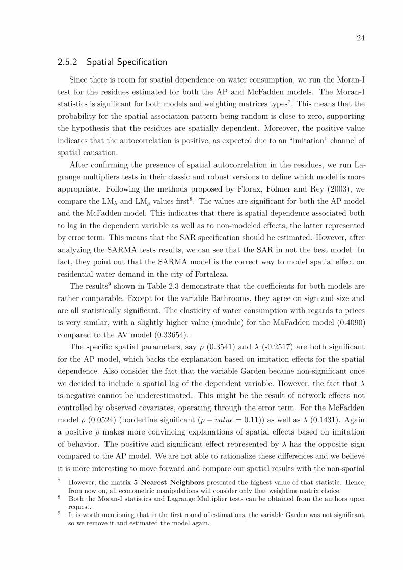
The results9 shown in Table 2.3 demonstrate that the coefficients for both models arerather comparable. Except for the variable Bathrooms, they agree on sign and size andare all statistically significant. The elasticity of water consumption with regards to pricesis very similar, with a slightly higher value (module) for the MaFadden model (0.4090)compared to the AV model (0.33654).

The specific spatial parameters, say ρ (0.3541) and λ (-0.2517) are both significantfor the AP model, which backs the explanation based on imitation effects for the spatialdependence. Also consider the fact that the variable Garden became non-significant oncewe decided to include a spatial lag of the dependent variable. However, the fact that λis negative cannot be underestimated. This might be the result of network effects notcontrolled by observed covariates, operating through the error term. For the McFaddenmodel ρ (0.0524) (borderline significant (p− value = 0.11)) as well as λ (0.1431). Againa positive ρ makes more convincing explanations of spatial effects based on imitationof behavior. The positive and significant effect represented by λ has the opposite signcompared to the AP model. We are not able to rationalize these differences and we believeit is more interesting to move forward and compare our spatial results with the non-spatial7 However, the matrix 5 Nearest Neighbors presented the highest value of that statistic. Hence,

from now on, all econometric manipulations will consider only that weighting matrix choice.8 Both the Moran-I statistics and Lagrange Multiplier tests can be obtained from the authors upon

request.9 It is worth mentioning that in the first round of estimations, the variable Garden was not significant,

so we remove it and estimated the model again.

25

Table 2.3 – Estimates Average Price and McFadden, with Spatial EffectsAverage Price Mc Fadden

Estimate S. E. Estimate S. E.Intercept 1.1166∗∗∗ 0.1122 1.6403∗∗∗ 0.0911log(Pavg) −0.3365∗∗∗ 0.0348 - -log(Pmg) - - −0.4090∗∗∗ 0.0318Diff - - 0.0389∗∗∗ 0.0012Income 0.0535∗∗∗ 0.0104 0.0442∗∗∗ 0.0081Male 0.1096∗∗∗ 0.0087 0.1102∗∗∗ 0.0074Female 0.0810∗∗∗ 0.0089 0.0650∗∗∗ 0.0069Bath 0.1194∗∗∗ 0.0131 0.0424∗∗∗ 0.0098Rho 0.3541∗∗∗ 0.0463 0.0524 0.0332lambda −0.2517∗∗∗ 0.0794 0.1431∗∗∗ 0.0422LR test 59.705∗∗∗ 45.84∗∗∗

Log likelihood -2432.501 -1351.896Source: Elaborated by the AuthorsNote: Signif. codes: 0 ∗∗∗ 0.001 ∗∗ 0.01 ∗ 0.05 . 0.1

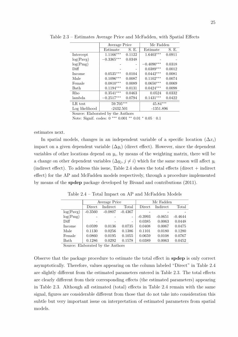
estimates next.In spatial models, changes in an independent variable of a specific location (∆xi)

impact on a given dependent variable (∆yi) (direct effect). However, since the dependentvariables of other locations depend on yi, by means of the weighting matrix, there will bea change on other dependent variables (∆yj, j 6= i) which for the same reason will affect yi(indirect effect). To address this issue, Table 2.4 shows the total effects (direct + indirecteffect) for the AP and McFadden models respectively, through a procedure implementedby means of the spdep package developed by Bivand and contributions (2011).

Table 2.4 – Total Impact on AP and McFadden ModelsAverage Price Mc Fadden

Direct Indirect Total Direct Indirect Totallog(Pavg) -0.3560 -0.0807 -0.4367 - - -log(Pmg) - - - -0.3993 -0.0651 -0.4644Diff - - - 0.0385 0.0063 0.0448Income 0.0599 0.0136 0.0735 0.0408 0.0067 0.0475Male 0.1130 0.0256 0.1386 0.1101 0.0180 0.1280Female 0.0860 0.0195 0.1055 0.0659 0.0108 0.0767Bath 0.1286 0.0292 0.1578 0.0389 0.0063 0.0452Source: Elaborated by the Authors

Observe that the package procedure to estimate the total effect in spdep is only correctasymptotically. Therefore, values appearing on the column labeled “Direct” in Table 2.4are slightly different from the estimated parameters entered in Table 2.3. The total effectsare clearly different from their corresponding effects (the estimated parameters) appearingin Table 2.3. Although all estimated (total) effects in Table 2.4 remain with the samesignal, figures are considerable different from those that do not take into consideration thissubtle but very important issue on interpretation of estimated parameters from spatialmodels.

26

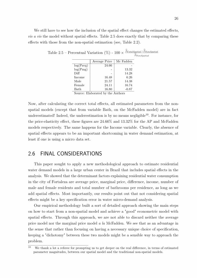
We still have to see how the inclusion of the spatial effect changes the estimated effects,vis a vis the model without spatial effects. Table 2.5 does exactly that by comparing theseeffects with those from the non-spatial estimation (see, Table 2.2).

Table 2.5 – Percentual Variation (%) - 100× βT otalSpatial−βNonSpatial

βNonSpatial

Average Price Mc Faddenlog(Pavg) 24.66 -log(Pmg) - 13.32Diff - 14.28Income 16.48 6.26Male 21.57 14.38Female 24.11 16.74Bath 16.80 -0.87Source: Elaborated by the Authors

Now, after calculating the correct total effects, all estimated parameters from the non-spatial models (except that from variable Bath, on the McFadden model) are in factunderestimated! Indeed, the underestimation is by no means negligible10. For instance, forthe price-elasticity effect, these figures are 24.66% and 13.32% for the AP and McFaddenmodels respectively. The same happens for the Income variable. Clearly, the absence ofspatial effects appears to be an important shortcoming in water demand estimation, atleast if one is using a micro data set.

2.6 FINAL CONSIDERATIONSThis paper sought to apply a new methodological approach to estimate residential

water demand models in a large urban center in Brazil that includes spatial effects in theanalysis. We showed that the determinant factors explaining residential water consumptionin the city of Fortaleza are average price, marginal price, difference, income, number ofmale and female residents and total number of bathrooms per residence, as long as weadd spatial effects. Most importantly, our results point out that not considering spatialeffects might be a key specification error in water micro-demand analysis.

Our empirical methodology built a sort of detailed approach showing the main stepson how to start from a non-spatial model and achieve a "good" econometric model withspatial effects. Through this approach, we are not able to discard neither the averageprice model nor the marginal price model a la McFadden. We see that as an advantage inthe sense that rather than focusing on having a necessary unique choice of specification,keeping a "dichotomy" between these two models might be a sensible way to approach theproblem.10 We thank a lot a referee for prompting us to get deeper on the real difference, in terms of estimated

parameter magnitudes, between our spatial model and the traditional non-spatial models.

27

As expected, for both spatial and non-spatial specifications, the average and marginalprices variables had a negative impact on water consumption. Also, water behaved as anormal good. Income, total of male and female residents, and total of bathrooms resultedin a positive effect. As to the long debate on endogeneity issues, we found no considerabledifferences between the AP and McFadden models. Interestingly, we were able to find theintramarginal effect (see Nordin (1976)).

Lagrange multipliers and SARMA tests showed both in classic and robust versionsthat the “best specification” to estimate residential water demand is the SARMA model,instead of the SEM. We address that by estimating a SARMA model for both the averageprice and the McFadden procedure. Now, after correcting the direct and indirect effects ofthe estimated parameters, the advantage of using a spatial approach appears to be moreevident. Not including spatial features underestimates almost all variables in absoluteterms when compared to their non-spatial counterparts. For instance, including spatialeffects increases the price-elasticity in the AP price in 24.66% and the price-elasticity forthe McFadden model in 13.32%!

As suggestions for future studies, we believe that both the incorporation of spatialheterogeneity and the inclusion of water quality variables are worth pursuing. Also, adetailed study of spatial effects on markets that are not well served by water companiesand that rely on alternative non-market sources of water seems to be a mandatory task.Another interesting line of research would be applying spatial models to longitudinal data.Finally, replicating our empirical exercise on different data sets coming from differentinstitutional backgrounds might be something worth pursuing in order to validate ourapproach.

REFERENCES

AGTHE, D. E.; BILLINGS, R. B.; DOBRA, J. L. A simultaneous equation demandmodel for block rates. Water Resources Research, v. 1, p. 1 – 4, 1986.

ANDRADE, T. et al. Saneamento urbano: a demanda residencial por água. Pesquisa ePlanejamento Econômico, v. 25, n. 3, p. 427–448, 1995.

ANSELIN, L. Spatial econometrics: methods and models. [S.l.: s.n.], 1988. 304 p. ISBN978-90-247-3735-2.

ANSELIN, L. Local indicators of spatial association-lisa. Geographical analysis, v. 27, n. 2,p. 93–115, 1995.

ARBUÉS, F.; GARCÍA-VALIÑAS, M. A.; ESPIÑEIRA, R. M. Estimation of residentialwater demand: a state-of-the-art review. Journal of Socio-Economics, v. 32, n. 1, p.81–102, 2003.

BIVAND, R.; CONTRIBUTIONS with. spdep: spatial dependence: weightingschemes, statistics and models. [S.l.], 2011. R package version 0.5-40. Disponível em:<http://CRAN.R-project.org/package=spdep>.

CHANG, H.; PARANDVASH, G. H.; SHANDAS, V. Spatial variations of single-familyresidential water consumption in portland, oregon. Urban Geography, v. 31, n. 7, p.953–972, 2010.

CORRADO, L.; FINGLETON, B. Where is the economics is spatial econometrics?Journal of Regional Science, Wiley Blackwell (Blackwell Publishing), v. 52, n. 2, p.210–239, May 2012.

DHARMARATNA, D.; HARRIS, E. Estimating residential water demand using thestone-geary functional form: the case of sri lanka. Water Resources Management, SpringerNetherlands, v. 26, n. 8, p. 2283–2299, 2012. ISSN 0920-4741.

FLORAX, R.; FOLMER, H.; REY, S. Specification searches in spatial econometrics: therelevance of hendry’s methodology. Regional Science and Urban Economics, Elsevier,v. 33, n. 5, p. 557–579, 2003.

FRANCZYK, J.; CHANG, H. Spatial analysis of water use in oregon, usa, 1985-2005.Water Resources Management, v. 23, n. 4, p. 755–774, 2009.

GOTTLIEB, M. Urban domestic demand of water in the united states. Land Economics,v. 39, n. 2, p. 204–210, 1963.

29

HOUSE-PETERS, L.; PRATT, B.; CHANG, H. Effects of urban spatial structure,sociodemographics, and climate on residential water consumption in hillsboro, oregon.JAWRA Journal of the American Water Resources Association, v. 46, n. 3, p. 461–472,2010.

HOWE, C. W.; LINAWEAVER, F. P. The impact of price on residential water demandand its relation to system design and price structure. Water Resources Research, v. 3, n. 1,p. 13, 1967.

JANMAAT, J. Spatial patterns and policy implications for residential water use: Anexample using kelowna, british columbia. Water Resources and Economics, Elsevier, v. 1,p. 3–19, Jan 2013.

JONES, C. V.; MORRIS, J. R. Instrumental price estimates and residential water demand.Water Resources Research, Wiley Blackwell (John Wiley & Sons), v. 20, n. 2, p.197–202, Feb 1984.

MATTOS, Z. d. B. Uma análise da demanda residencial por água usando diferentesmétodos de estimação. Pesquisa and Planejamento Econômico, v. 28, n. 1, p. 207–224,1998.

MCFADDEN, D.; PUIG, C.; KIRSCHNER, D. Determinants of the long-run demand forelectricity. In: Proceedings of the American Statistical Association. [S.l.: s.n.], 1977. v. 1,n. 1, p. 109–19.

MELO, J.; NETO, P. Estimação de funções de demanda residencial de agua em contextode preços não-lineares. Pesquisa and Planejamento Econômico, v. 37, n. 1, p. 149–173,2007.

MIYAWAKI, K.; OMORI, Y.; HIBIKI, A. Exact estimation of demand functions underblock rate princing. Econometric Reviews, 2013.

MOFFITT, R. The econometrics of piecewise-linear budget constraints: a survey andexposition of the maximum likelihood method. Journal of Business & Economic Statistics,JSTOR, v. 4, n. 3, p. 317–328, 1986.

NORDIN, J. A proposed modification of taylor’s demand analysis: comment. The BellJournal of Economics, v. 7, n. 2, p. 719–721, 1976.

OLMSTEAD, S. M.; HANEMANN, W. M.; STAVINS, R. N. Water demand underalternative price structures. Journal of Environmental Economics and Management,Elsevier, v. 54, n. 2, p. 181–198, Sep 2007.

OPALUCH, J. J. A test of consumer demand response to water prices: reply. LandEconomics, v. 60, n. 4, p. 417–421, 1984.

30

POLYCARPOU, A.; ZACHARIADIS, T. An econometric analysis of residential waterdemand in cyprus. Water Resources Management, Springer Netherlands, v. 27, n. 1, p.309–317, 2013. ISSN 0920-4741.

RAMACHANDRAN, M.; JOHNSTON, R. J. Quantitative restrictions and residentialwater demand : a spatial analysis of neighborhood effects. 2011.

RIETVELD, P.; ROUWENDAL, J.; ZWART, B. Block rate pricing of water in indonesia:an analysis of welfare effects. Bulletin of Indonesian Economic Studies, Informa UK(Taylor & Francis), v. 36, n. 3, p. 73–92, Dec 2000.

SALETH, R. M.; DINAR, A. Preconditions for market solution to urban water scarcity:empirical results from hyderabad city, India. Water Resources Research, Wiley Blackwell(John Wiley & Sons), v. 37, n. 1, p. 119–131, Jan 2001.

WENTZ, E. a.; GOBER, P. Determinants of small-area water consumption for the city ofphoenix, arizona. Water Resources Management, v. 21, n. 11, p. 1849–1863, 2007.

WORTHINGTON, A. C.; HOFFMAN, M. An empirical survey of residential waterdemand modelling. Journal of Economic Surveys, v. 22, n. 5, p. 842–871, Dec 2008.

3 SPATIAL WILLINGNESS TO PAY FORA FIRST-ORDER STOCHASTIC REDUC-TION ON THE RISK OF ROBBERY

3.1 INTRODUCTIONContingent Valuation (CV) is a method widely used in recent decades. Its foremost

objective is to infer, by means of public opinion surveys, the value of certain goodswhich are not readily tradable on traditional markets, such as public goods and naturalresources. This method consists in constructing a hypothetical market for a certain good,as realistic and structured as possible, such that, by performing a survey, researchers canextract the maximum willingness to pay (WTP) of individuals for that good1. Bowen(1943) and Ciriacy-Wantrup (1947) were the pioneers to propose the use of public opinionsurveys specially developed for the valuation of social goods or collective goods (CARSON;HANEMANN, 2005). These authors believed that voting would be the closest substituteto consumer choice, so they considered that the public opinion surveys would be a validinstrument for valuation of these goods (HOYOS; MARIEL, 2010; CARSON; HANEMANN,2005).

Although the main goal of CV is to measure the monetary value of a certain good foran individual (CARSON; HANEMANN, 2005), there is a much more powerful insight ontop of it: welfare analysis. According to Hoyos and Mariel (2010), by means of CV surveys,it is possible to directly obtain a monetary measure (Hicksian) of welfare associated witha discrete change in the provision of an environmental good, either by the substitution ofone good for another or by the marginal substitution of different attributes of an existinggood.

To understand the measurement of this value for the agent, we follow Whiteheadand Blomquist (2006) and Carson and Hanemann (2005). Define a utility function that,for simplicity, only depends on a good x and contingent good q, given by u(x, q). Thus,assuming that good q is desirable, and that q0 is the state in which the consumer doesnot have the good and q1 is the state in which the consumer has access to the good,the consumer will pay to consume the good if, and only if, the utility obtained with theconsumption of the good is greater than the utility obtained without the consumption ofthe good, i.e., u1(x, q1) > u0(x, q0).1 There is also the concept of minimum willingness to accept, where the individual reports the minimum

amount he/she would be willing to accept to give up consuming a good that he/she would have beenentitled. However, we will not cover this side.

32

So, the consumer will maximize their utility function u(x, q), subject to their budgetconstraint, given by y = px+ tq, where y is the consumer’s income, p is the price of goodx and t is the price of contingent good q, to define the optimal level of consumption ofgoods x and q. From this, we find the indirect utility function, denoted by v(p, q, y), whoseusual properties with respect to p and y are satisfied. On the other hand, solving theproblem of minimizing costs, subject to the constraint level of utility in state q0, generatesan expenditure function given by e(p, q, u), (see Mas-Colell, Whinston and Green (1995)).According to Carson and Hanemann (2005), the value for the individual, in monetaryterms, of the increment in utility caused by the change of state from q0 to q1 can berepresented by two Hicksian measures: the compensatory variation and the equivalentvariation. As shown by (MAS-COLELL; WHINSTON; GREEN, 1995). Formally, thosemeasures are solutions to the following equations:

v1(p, q1, y − C) = v0(p, q0, y) (3.1)

v1(p, q1, y) = v0(p, q0, y + E) (3.2)

Based on these two concepts, one can define the willingness to pay in two different ways:i) as the difference between expenditure functions in the situation without contingentgood and with contingent good, and, ii) as the monetary value that leaves the consumerindifferent between the status quo and the increase in the provision of contingent good.Following Carson and Hanemann (2005), it is possible to define the willingness to pay’sfunction as a function to initial value q0, the terminal value, q1, and the values of p and yin which the changes in q occur.

However, a common assumption for both C(q0, q1, p, y) or E(q0, q1, p, y) is the fact thatwhat is measured is a discrete change between two deterministic states of nature withdegenerate distribution, i.e., from initial value q0 (status quo) with Prob(q0) = 1 up to theterminal value, q1 with Prob(q1) = 1. The more general and interesting case of measuringwillingness to pay for changes between (non-degenerate) lotteries of states of nature arestill lacking a complete approach in the literature, although Cameron, DeShazo and Stiffler(2010) and Cameron and DeShazo (2013) are notably exceptions.

Although the scope of applicability of the CV method has grown considerably, manykey areas traditionally approached by economists have not been thoroughly touched uponby contingent valuation. A notable example is the economics of crime. Since problems ofmeasurement, externalities, and difficulties in assessing costs plague the area of crime andeconomics, it appears to us that underutilization of CV methods is hard to understand.In fact, very few papers have applied that method so far.

Ludwig and Cook (2001) estimate the benefits of reducing crime using CV methods.They focus on gun violence, in a national survey in the U.S. Using a parametric form, theyfound a value of US$ 24.5 billion as the worth for American society for a 30% reduction

33

in gun violence or US$1.2 million per injury avoided. Still in the U.S., Cohen et al.(2004) using a nationally representative sample of 1,300 U.S. residents, found that therepresentative American household would be willing to pay between US$ 100 and US$ 150per year for programs that reduced specific crimes by 10% in their communities. Cohen etal. (2004) analyzed five types of crimes: burglary, serious assault, armed robbery, rape orsexual assault and murder.

In the U.K., Atkinson, Healey and Mourato (2005) valued the costs of three violentcrimes: common assault (no injury), other wounding (moderate injury) and seriouswounding (serious injury). Their data set contained 807 observations in Wales and inEngland. At the interview, respondents were told that the probability of being victimsof each crime was 4% for common assault and 1% for both other wounding and seriouswounding. Then each respondent was asked to express his WTP to reduce their chance ofbeing victims of this offense by 50% over the next 12 months. The estimated values forWTP were £ 105.63, £ 154.54 and £ 178.33 for common assault, other wounding andserious wounding, respectively.

Finally, in Portugal, Soeiro and Teixeira (2010) studied the determinants of highereducation students’ willingness to pay for reducing the risk of being victims of violentcrimes. They conducted an online survey with students from the University of Porto, whichhad 1,122 respondents. By means of a parametric approach, they modeled WTP as afunction of demographic factors (age and gender), family-related factors (income, dimension,dependents), degree (undergraduate, master, PhD) and field of study (economics, arts, ...),crime-related factors (crime victim, crime time, physical injuries, psychological damages,fear of crime), averting behavior (locking doors), payment vehicle and policy. They foundthat variables such as age and family members had a negative impact in WTP, whereasvariables such as gender, fear of crime, locking doors and payment vehicle had a positiveimpact on willingness to pay.

In Brazil, Araújo and Ramos (2009) used contingent valuation to estimate the lossof welfare associated with insecurity, by means of willingness to pay. The survey wasconducted in the city of João Pessoa (PB), and had 400 observations. Respondents wereasked how much they would be willing to pay for a bundle of public security services,which includes: fixed police posts equipped with adequate weaponry; vehicles equippedfor better care and effective police action; trained officers, with greater integration withthe community and greater agility (speed) in citizen service; day and night patrols andconduction of educational programs to prevent violence and crime. They found that publicsecurity is a normal and common good and also that the estimated cost of insecurity inJoão Pessoa varies between R$ 6,524,727.01, considering the most conservative estimative,and R$ 104,864,863.52 for the highest value.

Although Ludwig and Cook (2001), Cohen et al. (2004), Atkinson, Healey and Mourato(2005), and Soeiro and Teixeira (2010) propose valuations between non-degenerate lotteries,

34

they stopped very far from building an econometric model that incorporates the basictenets of choice under risk.

Given that state of affairs, say, the lack of a conceptual empirical strategy for CVamong lotteries, and incipient literature on willingness to pay for crime reduction policies,our main contributions are: i) to build (and estimate) an econometric model capable ofassessing the willingness to pay for first-order stochastic reductions in the risk of robbery,ii) to incorporate, in a sensible and manageable way, spatial effects to realistic mimicsinteractions present in a large and densely populated urban center in Brazil, and, iii) toapply our empirical strategy to real data, more specifically, to Brazilian data.

We believe to have succeeded in a satisfactory way. We make use of a unique geo-referenced sample of 4,030 households from the city of Fortaleza, CE (Brazil), containinginformation on socioeconomic background, experience, expectation of victimization, andwillingness to pay to reduce some type of crimes (see, Carvalho (2012)). For the globalmodel (i.e., without spatial effects), the parameters for all independent variables, exceptAge, show positive signs. Older people tend to pay less to reduce crime than young peopledo, men and more educated people tends to pay more for risk reductions. Finally, as tovariables of perception and experience of victimization (variable Perception of patrollingis measured in decreasing order), the lower the perception of patrolling, the greater thewillingness to pay to reduce the number of robberies, and people who were Victims ofrobbery tend to pay more to prevent such experience again. We also estimated an averagewillingness to pay of R$ 23.35 per month/household, a value of R$ 5.91 higher than theestimated value of the nonparametric form. Also, we estimated the implicit value of astatistical robbery approximately equal to R$ 11,969 per crime avoided. Both valuesare quite reasonable. As a matter of fact, our proposed specification made possible toimplicitly estimate the average cost of each robbery in the city of Fortaleza. This amountsto approximately 4,15% of the income. Multiplying this value by average income, we havea value of R$ 61,38 per robbery.

The full spatial heterogeneity reveals our local model. By means of a geographicallyweighted regression (GWR), it is possible to allow for the estimation of local parametersrather than global parameters (FOTHERINGHAM; BRUNSDON; CHARLTON, 2003).Now, the main difference is the lack of one estimated parameter for each independentvariable. Instead, for each independent variable, we have a possible different parameter foreach sampled point. Overall, the estimated spatial heterogeneity brings us both expectedresults and surprises. The estimative mapping for variables Gender, Age and Educationpresent a reasonable amount of spatial heterogeneity and, as expected, follow the veryinertial city’s socioeconomic spatial distribution profile. Given the geographically weightedregression, we implement a protocol to calculate a surface of willingness to pay. In orderto do that, we apply Kriging techniques. The image that emerges from such empiricalexercise is not difficult to rationalize: the income, age, and crime spatial distribution of

35

Fortaleza has an important effect on the surface of willigness to pay. Although peripheriespresent lower willingness to pay, as long as we go inwards, there is plenty of heterogeneityon the spatial distribution of willingness to pay for robbery reduction. It is worth notingthat the highest willingness to pay is not necessarily the richest one, corroborating with atheory of crime that posits an active role for victim (costly) precautions.

Besides this introduction, we have more 5 Sections. Section (3.2) introduces the dataset used in our estimatives. Section (3.3) develops a simple structural model of contingentchoice between risky lotteries and frames the resulting equation as a fully parametriceconometric model, although, given the type of data collected, we end up estimatingit by fully maximum likelihood. In order to introduce our spatial effects, Section (3.4)deals with geographically weighted regression and how to manage that in our context.We call such model local to contrast with the previous one that neglects spatial effects.All estimatives are performed on Section (3.5), as well as their interpretations. Finally,Section (3.6) elaborates more on results and proposes futures improvements.

3.2 DATA SETOur data set comes from a survey conducted in 2012 where a total of 4,030 households

were sampled along 119 districts (bairros) from the city of Fortaleza (Brazil) during themonths of October 2011 to January 2012, see Carvalho (2012). Besides information aboutsocioeconomic background, experience and expectation of victimization, Carvalho (2012)induced respondents to express their willingness to pay to reduce certain types of crimes.A key component from the data set is due to the fact that household, work and schoolpositions were georeferenced.

The section about contingent valuation presents respondents with a fictional scenariowhere there was a program to fight against criminality, more specifically the crime ofrobbery. The respondent was informed that the program was successful and succeeded inreducing 50% the amount of robberies. However, to maintain this program, it was necessarythat the population funds it by means of fictitious future taxes. Then, respondents wereasked if they were willing to pay a monthly fee to maintain that crime prevention program,and if so, how much they would be willing to pay monthly. The exact introduction andquestion wording were:

•Introductory Remark: Now I would like to know how much you are willing to spendto reduce certain crimes in your town. In each case, I will ask you to answer whetheryou would vote ‘’yes” or ‘’no” for a bill that would require from you and from eachhousehold in your community a payment to prevent certain crimes. Remember thatthe money you agree to spend to prevent crimes is the same that you could use tobuy food, clothes or other needs to you and to your family.

36

•Question: Q105 Now forget about this program that was able to reduce homicidesand think about a new one. Let’s suppose a new government program funded by thepopulation of Fortaleza managed to cut the occurrence of personal robbery in the cityin half. Would you be willing to pay a monthly amount to keep this program of crimeprevention?

Table 3.1 defines the variables used in this paper. Initially, we show the socioeconomicprofile, the perception of security and experience of victimization of the research partic-ipants. From a total of 4,030 observations in the initial sample, 246 observations wereremoved due to lack of information about participation in the program and due to thedifficulty in georeferencing respondents’ addresses. Table 3.2 shows that 44,66% of therespondents were men. The overall age of respondents was 39,45 years old, with completefundamental school level. As to income, its average level was R$ 1,488.70 per month, butabout 50% of respondents earn R$ 817.50 or less2.

Table 3.1 – Variables’ descriptions

Variable DescriptionGender 1 if male; 0 if femaleAge yearsIncome R$Education 1.No education; 2.Incomplete fundamental school; 3.Complete fun-

damental school; 4.Incomplete high school; 5.Complete high school;6.Incomplete undergraduate degree; 7.Complete undergraduatedegree; 8.Graduate Program

Victim of robbery 1 if you’ve been the victim of robbery; 0 OtherwiseSubject Prob. ∈ (0,1)Perception of patrolling 1.Always; 2.Often; 3.Sometimes ; 4.Rarely; 5.NeverWillingness to pay R$/monthSource: Elaborated by the Authors

As to victimization and perception of security, 23,24% of respondents were victimsof robbery at least once in the last five years. As to perception of security, on average,respondents considered that the probability of being robbed in the next 12 months wasabout 49.2%, although the perception of patrolling is frequent (mean 2.05).

Table 3.4 shows that out of 3,784 respondents, 1,709 (45,16%) answered that theyare willing to pay a monthly fee to fund the program to combat robberies, while 2,076(54,86%) answered they would not pay any amount. Despite the fact that the number ofpeople who are not willing to pay to keep the program to combat crime is fairly high, it isconsistent with other studies about contingent valuation, for instance, Atkinson, Healeyand Mourato (2005), which had 34,57%, and Araújo and Ramos (2009), which had a rateof 48.5 %, the last one for the city of João Pessoa (Brazil). This second group is definedin the contingent valuation literature as protesters. These people refuse to pay for a good2 The minimum wage in Brazil at the time of the survey was R$ 545,00.

37

Table 3.2 – Sample Description - Total

Variable Mean Std. dev Min Median Max NA NGender 0.4466 0.4972 0 0 1 0 3784Age 39.4519 16.8278 16 37 94 80 3704Income 1,488.70 1,524.27 272.50 817.50 10,900.00 137 3647Education 3.5552 1.6451 1 3 8 0 3784Victim of robbery 0.2324 0.4224 0 0 1 1 3783Subject Prob. 0.4920 0.2990 0 0.5000 1 532 3252Perception of patrolling 2.0533 1.2146 1 1 5 10 3774Source: Elaborated by the Authors

either because they think they already pay many taxes or, in the case of public goods,because the provision of such goods is responsibility of the government, or simply becauseit is the duty of other groups to pay for the provision of that good3. However, it is possiblethat someone reports a true zero value for the reduction on the risk of being robbed orjust cannot afford to pay for such amount.

Notwithstanding that, we will not enter in this debate4, and we simply characterizethem as protesters. The protesters’ group, 50.48% of them were men, with an average ageof 41.42 years old and with complete fundamental school level. In this group, the averageincome was equal to R$ 1,488.90, but 50% of them earned R$ 817.50 or less. Concerningthe expectation of victimization and perception of security, 22,74% of them suffered atleast one robbery in the last five years and they consider that the probability of beingrobbed in the next 12 month is about 48,47%, even though the perception of patrolling isfrequent. In the CV’s literature, the standard procedure for dealing with this group isto remove them from the sample and proceed to estimation of the maximum willingnessto pay (STRAZZERA et al., 2003). However, Strazzera et al. (2003) states that thisprocedure is valid only when both groups are similar due to the fact that, if this is not thecase, selection bias will pop up.

We compared the empirical distributions for both protesters and those who are willingto pay a positive amount of money and they are quite similar. Thus, protesters andthose who are willing to pay are quite homogeneous, which indicates that the estimates ofwillingness to pay using only the second group should not be affected by selection bias(STRAZZERA et al., 2003). Thus, we remove the group of protesters from the sample inorder to estimate the cost of robberies. Table 3.4 shows the characteristics of those whoare willing to pay to maintain the crime’s reduction program.

Table 3.5 shows the frequency distribution of willingness to pay. From the total of1,708 respondents who answered that they would accept to pay some amount to reducerobberies, 70 did not know/ did not want to inform a value from those presented in the3 We also consider the fact that individuals do not report their willingness to pay for fear that, once

answered a value, the research can be used to make them pay the reported amount.4 For details, see Jorgensen et al. (1999)

38

Table 3.3 – Sample description - Protesters

Variable Mean Std. dev Min Median Max NA NGender 0.5048 0.5001 0 1 1 0 2076Age 41.4205 17.4722 16 39 93 26 2050Income 1,488.90 1,553.82 272.50 817.50 10,900.00 84 1992Education 3.5111 1.6823 1 3 8 0 2076Victim of robbery 0.2274 0.4192 0 0 1 0 2076Subject Prob. 0.4847 0.2973 0 0.5000 1 302 1774Perception of patrolling 2.0778 1.2273 1 2 5 6 2070Fonte: Elaborated by the Authors

Table 3.4 – Sample description - Willing to Pay

Variable Mean Std. dev Min Median Max NA NGender 0.3759 0.4845 0 0 1 0 1708Age 37.0121 15.6586 16 34 94 54 1654Income 1,488.45 1,488.40 272.50 817.50 10,900.00 53 1655Education 3.6089 1.5976 1 4 8 0 1708Victim of robbery 0.2384 0.4262 0 0 1 1 1707Subject Prob. 0.5007 0.3008 0.0100 0.5000 1 230 1478Perception of patrolling 2.0235 1.1987 1 1 5 4 1704Source: Elaborated by the Authors

payment card. Thus, we had 1,638 observations. The columns Cumulative frequencyand Survival probability in table 3.5 indicate, respectively, the number of people and thepercentage of the sample that is willing to pay at least the indicated value. Thus, it canbe seen that 990 people, equivalent to 60.40%, are willing to pay at least R$ 10 for themaintenance of the combating robbery crimes program.

Table 3.5 – Willingness to pay frequency distribution

WTP Frequency Cumulative frequency Survival probability1 212 1638 1.00005 428 1426 0.870610 460 998 0.609315 159 538 0.328425 173 379 0.231450 123 206 0.125875 12 83 0.0507100 38 71 0.0433150 8 33 0.0201+150 25 25 0.0153Source: Elaborated by the Authors

One can also notice that, as the value of willingness to pay increases, fewer people will bewilling to pay this amount.

From this empirical distribution of willingness to pay, we estimated, nonparametrically,

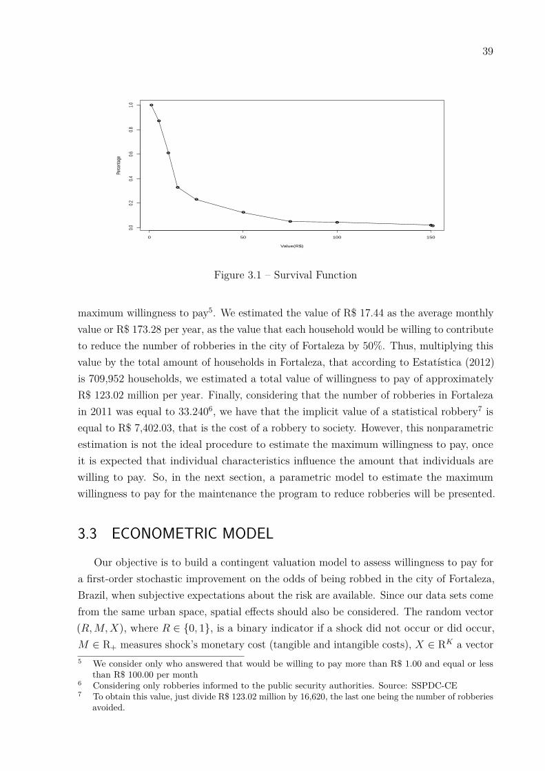
39

●●

●●

●

●

●

●

●

●

0 50 100 150

0.0

0.2

0.4

0.6

0.8

1.0

Value(R$)

Perc

enta

ge

Figure 3.1 – Survival Function

maximum willingness to pay5. We estimated the value of R$ 17.44 as the average monthlyvalue or R$ 173.28 per year, as the value that each household would be willing to contributeto reduce the number of robberies in the city of Fortaleza by 50%. Thus, multiplying thisvalue by the total amount of households in Fortaleza, that according to Estatística (2012)is 709,952 households, we estimated a total value of willingness to pay of approximatelyR$ 123.02 million per year. Finally, considering that the number of robberies in Fortalezain 2011 was equal to 33.2406, we have that the implicit value of a statistical robbery7 isequal to R$ 7,402.03, that is the cost of a robbery to society. However, this nonparametricestimation is not the ideal procedure to estimate the maximum willingness to pay, onceit is expected that individual characteristics influence the amount that individuals arewilling to pay. So, in the next section, a parametric model to estimate the maximumwillingness to pay for the maintenance the program to reduce robberies will be presented.

3.3 ECONOMETRIC MODELOur objective is to build a contingent valuation model to assess willingness to pay for

a first-order stochastic improvement on the odds of being robbed in the city of Fortaleza,Brazil, when subjective expectations about the risk are available. Since our data sets comefrom the same urban space, spatial effects should also be considered. The random vector(R,M,X), where R ∈ {0, 1}, is a binary indicator if a shock did not occur or did occur,M ∈ R+ measures shock’s monetary cost (tangible and intangible costs), X ∈ RK a vector5 We consider only who answered that would be willing to pay more than R$ 1.00 and equal or less

than R$ 100.00 per month6 Considering only robberies informed to the public security authorities. Source: SSPDC-CE7 To obtain this value, just divide R$ 123.02 million by 16,620, the last one being the number of robberies

avoided.

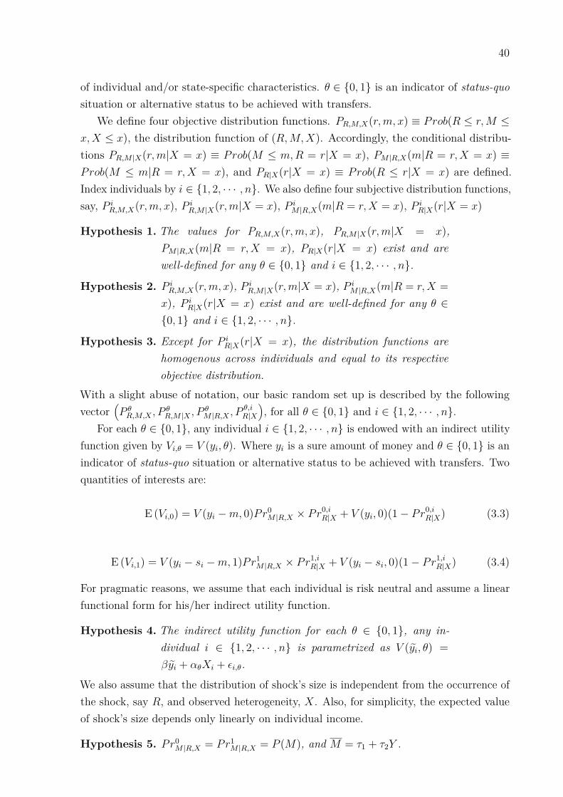
40

of individual and/or state-specific characteristics. θ ∈ {0, 1} is an indicator of status-quosituation or alternative status to be achieved with transfers.

We define four objective distribution functions. PR,M,X(r,m, x) ≡ Prob(R ≤ r,M ≤x,X ≤ x), the distribution function of (R,M,X). Accordingly, the conditional distribu-tions PR,M |X(r,m|X = x) ≡ Prob(M ≤ m,R = r|X = x), PM |R,X(m|R = r,X = x) ≡Prob(M ≤ m|R = r,X = x), and PR|X(r|X = x) ≡ Prob(R ≤ r|X = x) are defined.Index individuals by i ∈ {1, 2, · · · , n}. We also define four subjective distribution functions,say, P i

R,M,X(r,m, x), P iR,M |X(r,m|X = x), P i

M |R,X(m|R = r,X = x), P iR|X(r|X = x)

Hypothesis 1. The values for PR,M,X(r,m, x), PR,M |X(r,m|X = x),PM |R,X(m|R = r,X = x), PR|X(r|X = x) exist and arewell-defined for any θ ∈ {0, 1} and i ∈ {1, 2, · · · , n}.

Hypothesis 2. P iR,M,X(r,m, x), P i

R,M |X(r,m|X = x), P iM |R,X(m|R = r,X =

x), P iR|X(r|X = x) exist and are well-defined for any θ ∈

{0, 1} and i ∈ {1, 2, · · · , n}.

Hypothesis 3. Except for P iR|X(r|X = x), the distribution functions are

homogenous across individuals and equal to its respectiveobjective distribution.

With a slight abuse of notation, our basic random set up is described by the followingvector

(P θR,M,X , P

θR,M |X , P

θM |R,X , P

θ,iR|X

), for all θ ∈ {0, 1} and i ∈ {1, 2, · · · , n}.

For each θ ∈ {0, 1}, any individual i ∈ {1, 2, · · · , n} is endowed with an indirect utilityfunction given by Vi,θ = V (yi, θ). Where yi is a sure amount of money and θ ∈ {0, 1} is anindicator of status-quo situation or alternative status to be achieved with transfers. Twoquantities of interests are:

E (Vi,0) = V (yi −m, 0)Pr0M |R,X × Pr

0,iR|X + V (yi, 0)(1− Pr0,i

R|X) (3.3)

E (Vi,1) = V (yi − si −m, 1)Pr1M |R,X × Pr

1,iR|X + V (yi − si, 0)(1− Pr1,i

R|X) (3.4)

For pragmatic reasons, we assume that each individual is risk neutral and assume a linearfunctional form for his/her indirect utility function.

Hypothesis 4. The indirect utility function for each θ ∈ {0, 1}, any in-dividual i ∈ {1, 2, · · · , n} is parametrized as V (yi, θ) =βyi + αθXi + εi,θ.

We also assume that the distribution of shock’s size is independent from the occurrence ofthe shock, say R, and observed heterogeneity, X. Also, for simplicity, the expected valueof shock’s size depends only linearly on individual income.

Hypothesis 5. Pr0M |R,X = Pr1

M |R,X = P (M), and M = τ1 + τ2Y .

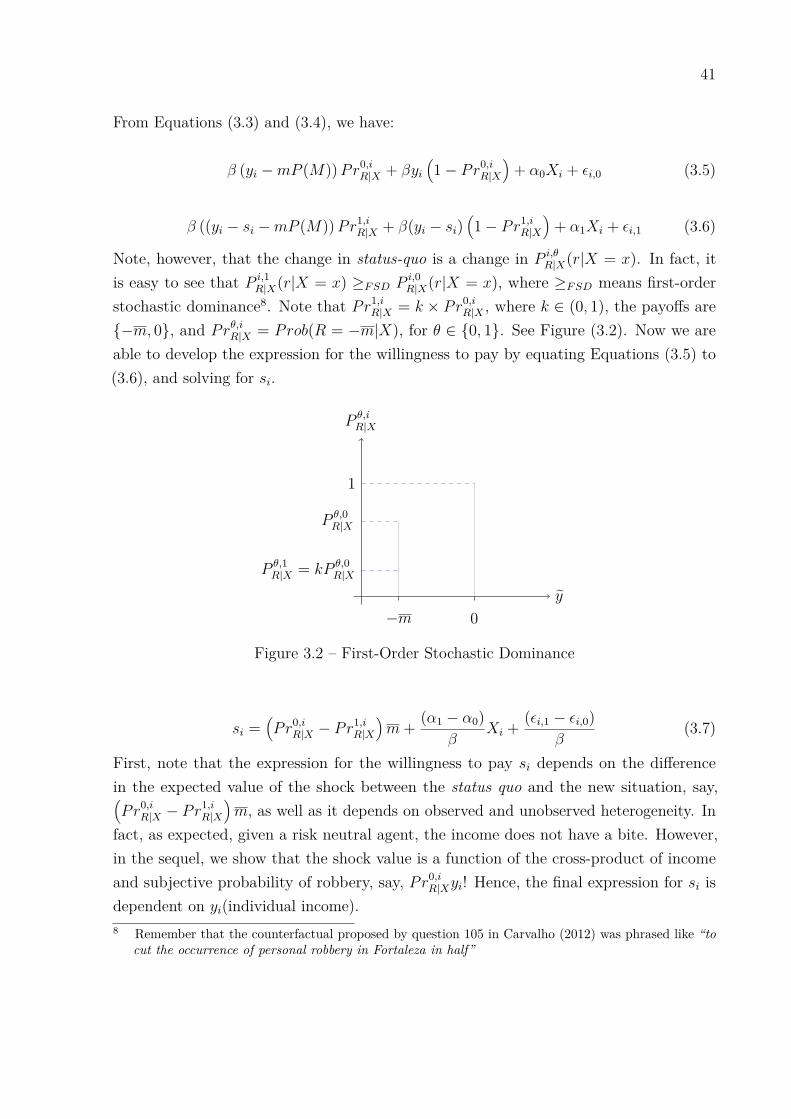
41

From Equations (3.3) and (3.4), we have:

β (yi −mP (M))Pr0,iR|X + βyi

(1− Pr0,i

R|X

)+ α0Xi + εi,0 (3.5)

β ((yi − si −mP (M))Pr1,iR|X + β(yi − si)

(1− Pr1,i

R|X

)+ α1Xi + εi,1 (3.6)

Note, however, that the change in status-quo is a change in P i,θR|X(r|X = x). In fact, it

is easy to see that P i,1R|X(r|X = x) ≥FSD P i,0

R|X(r|X = x), where ≥FSD means first-orderstochastic dominance8. Note that Pr1,i

R|X = k × Pr0,iR|X , where k ∈ (0, 1), the payoffs are

{−m, 0}, and Prθ,iR|X = Prob(R = −m|X), for θ ∈ {0, 1}. See Figure (3.2). Now we areable to develop the expression for the willingness to pay by equating Equations (3.5) to(3.6), and solving for si.

y

P θ,iR|X

−m 0

1

P θ,0R|X

P θ,1R|X = kP θ,0

R|X

Figure 3.2 – First-Order Stochastic Dominance

si =(Pr0,i

R|X − Pr1,iR|X

)m+ (α1 − α0)

βXi + (εi,1 − εi,0)

β(3.7)

First, note that the expression for the willingness to pay si depends on the differencein the expected value of the shock between the status quo and the new situation, say,(Pr0,i

R|X − Pr1,iR|X

)m, as well as it depends on observed and unobserved heterogeneity. In

fact, as expected, given a risk neutral agent, the income does not have a bite. However,in the sequel, we show that the shock value is a function of the cross-product of incomeand subjective probability of robbery, say, Pr0,i

R|Xyi! Hence, the final expression for si isdependent on yi(individual income).8 Remember that the counterfactual proposed by question 105 in Carvalho (2012) was phrased like “to

cut the occurrence of personal robbery in Fortaleza in half”

42

Remember that Pr1,iR|X = k × Pr0,i

R|X , and m = τ1 + τ2yi. Defining α ≡ (α1−α0)β

, andεi ≡ (εi,1−εi,0)

β, and Zi ≡ (1 − k)Pr0,i

R|X , Wi ≡ Ziyi we get the estimable equation, where,with no loss of generality, right-hand side variable appears in logarithmic form:

ln(si) = ln (τ1Zi + τ2Wi + αXi) + εi (3.8)

Where, εi ∼ N(0, σ2). Approximating the left-hand side of Equation (3.8) by a first orderTaylor’s expansion (Note that the full Taylor’s approximation is ln(x) = (x− 1)− (x−1)2

2 +(x−1)3

3 − (x−1)4

4 · · · , as long as we re-scale monetary values si to belong to the interval(−1, 1] actually close to 1, we get:

ln(siθ

)= ln

(τ1

θZi + τ2

θWi + α

θXi

)+ εi (3.9)

Where θ ∈ (min(si),max(si)). Assuming that Xi has an intercept whose parameter isαintercpt

β:

ln(si) =(αintercpt

β+ ln(θ)− 1

)+ τ1

θZi + τ2

θWi + α

θXi + εi (3.10)

Before we proceed, it is worth noting that models which incorporate willingness to pay forfirst-order stochastic dominance improvements on risks is a quite new endeavor. In fact,there are only two papers we are aware of, say, Cameron, DeShazo and Stiffler (2010) andCameron and DeShazo (2013), that build on this topic. Their approach is different fromours, however. Last, but not least, it is important to stress that individual’s subjectiveexpectations play a crucial role in our modeling strategy.

So, Cameron and Huppert (1989) propose that contingent valuation data sets obtainedby means of payment cards’ method can be analyzed parametrically by means of maximumlikelihood models with data in intervals. They suggest that when an agent chooses avalue in payment card, say tui, the true value of the agent’s willingness to pay is greaterthan or equal to this value, but less than the next card value, say tu+1i. Therefore, theprobability that the agent chooses to pay the tui value is equal to the probability that thetrue willingness to pay is in the range defined by tui and tu+1i.

P (tui) = P (tui ≤ s < tu+1i) (3.11)

Thus, it is possible to rewrite 3.11 as:

P (tui) = P (log(tui) ≤ log(si) < log(tu+1i)) (3.12)

By equation 3.10, we have that s has mean µ and standard deviation σ. Then, defineµ as:

µ =(αintercpt

β+ ln(θ)− 1

)+ τ1

θZi + τ2

θWi + α

θXi (3.13)

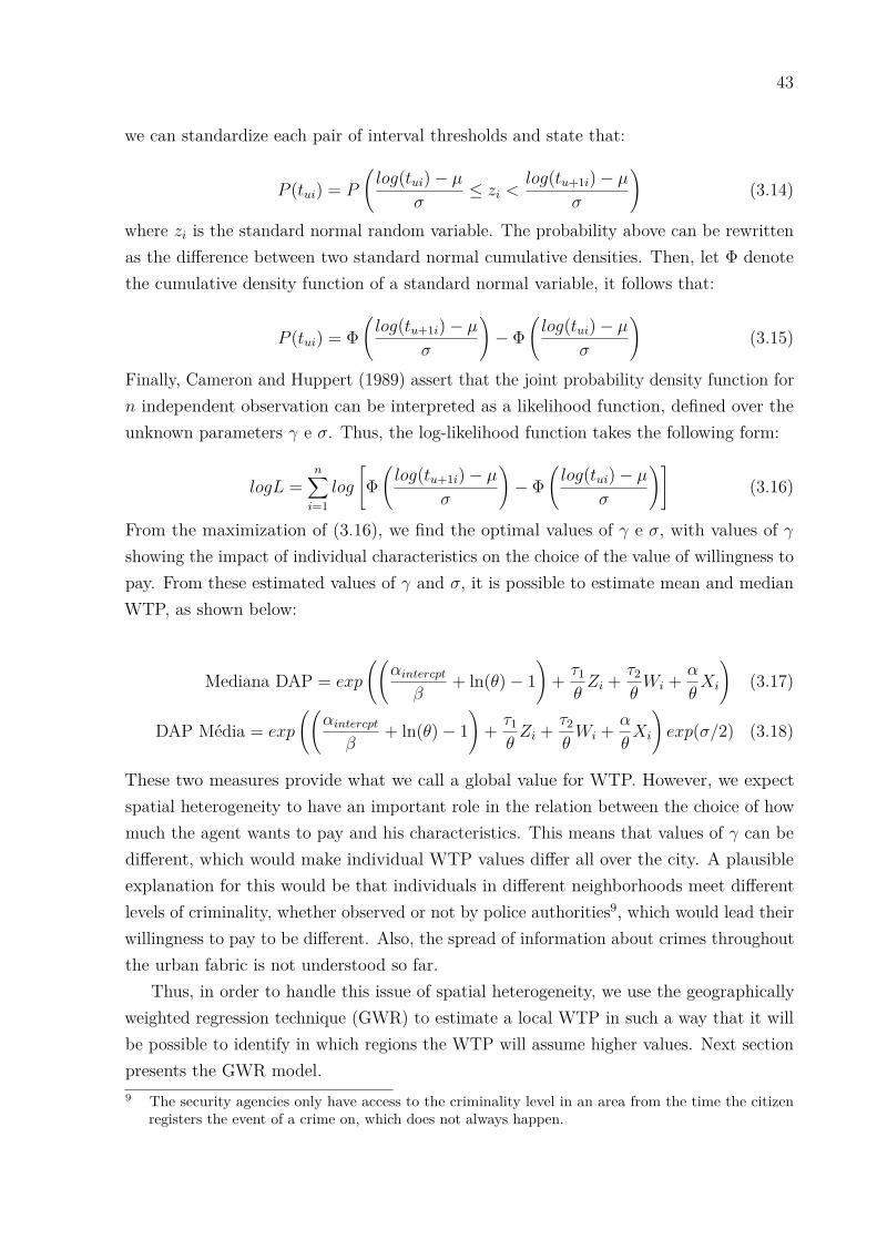
43

we can standardize each pair of interval thresholds and state that:

P (tui) = P

(log(tui)− µ

σ≤ zi <

log(tu+1i)− µσ

)(3.14)

where zi is the standard normal random variable. The probability above can be rewrittenas the difference between two standard normal cumulative densities. Then, let Φ denotethe cumulative density function of a standard normal variable, it follows that:

P (tui) = Φ(log(tu+1i)− µ

σ

)− Φ

(log(tui)− µ

σ

)(3.15)

Finally, Cameron and Huppert (1989) assert that the joint probability density function forn independent observation can be interpreted as a likelihood function, defined over theunknown parameters γ e σ. Thus, the log-likelihood function takes the following form:

logL =n∑i=1

log

[Φ(log(tu+1i)− µ

σ

)− Φ

(log(tui)− µ

σ

)](3.16)

From the maximization of (3.16), we find the optimal values of γ e σ, with values of γshowing the impact of individual characteristics on the choice of the value of willingness topay. From these estimated values of γ and σ, it is possible to estimate mean and medianWTP, as shown below:

Mediana DAP = exp

((αintercpt

β+ ln(θ)− 1

)+ τ1

θZi + τ2

θWi + α

θXi

)(3.17)

DAP Média = exp

((αintercpt

β+ ln(θ)− 1

)+ τ1

θZi + τ2

θWi + α

θXi

)exp(σ/2) (3.18)

These two measures provide what we call a global value for WTP. However, we expectspatial heterogeneity to have an important role in the relation between the choice of howmuch the agent wants to pay and his characteristics. This means that values of γ can bedifferent, which would make individual WTP values differ all over the city. A plausibleexplanation for this would be that individuals in different neighborhoods meet differentlevels of criminality, whether observed or not by police authorities9, which would lead theirwillingness to pay to be different. Also, the spread of information about crimes throughoutthe urban fabric is not understood so far.

Thus, in order to handle this issue of spatial heterogeneity, we use the geographicallyweighted regression technique (GWR) to estimate a local WTP in such a way that it willbe possible to identify in which regions the WTP will assume higher values. Next sectionpresents the GWR model.9 The security agencies only have access to the criminality level in an area from the time the citizen

registers the event of a crime on, which does not always happen.

44

3.4 A “LOCAL” ECONOMETRIC MODELAccording to Almeida (2012), analyzing only the average or global response of a

phenomenon may not be useful or convenient, since socioeconomic phenomena are notlikely to be constant in different regions. Fotheringham, Brunsdon and Charlton (2003)refer to this situation as spatial non-stationarity and claim that any relationship that isnon-stationary over space is not well represented by a global statistic and, indeed, thisglobal value may be very misleading locally.

Fotheringham, Brunsdon and Charlton (2003) affirm that there are several reasons toexpect that a relationship varies over space. Among possible explanations, we can citesample variations, misspecification and, most importantly, there might be relationshipswhich are intrinsically different across space. In the last case, it is suggested that there arespatial variations in peoples’ attitudes or preferences or there are different administrative,political or other contextual issues that produce different responses to the same stimuliover space.

When it comes to the object of study in this article, it is a stylized fact that crimedistribution is heterogenous across space. In big cities, like Fortaleza (the fifth largest cityin Brazil with an area of 313 square kilometers, boasting one of the highest demographicdensities in the country, say, 8,001 per km2), robberies are concentrated on richer areas inthe city, leading to formation of crime clusters in these areas. Due to this heterogeneousdistribution, we expected that individuals’ reactions to crime would also be heterogeneous.So, we expect that an individual who lives in a region with high rates of criminalityhas a different behavior than an individual who lives in low crime prone regions. Thus,unlike classical models of spatial dependence, here we do not expect that individuals caninfluence each other’s willingness to pay, but we expected that different individuals havedifferent factors that influence their willingness to pay. So, a variable that can influence thewillingness to pay for individual i maybe have no influence on individual j, or have moreor less influence. In this sense, a local model is necessary to estimate this relationship.

The geographically weighted regression (GWR) is a method that extends the tradi-tional regression framework by allowing the estimation of local parameters rather thanglobal parameters (FOTHERINGHAM; BRUNSDON; CHARLTON, 2003). This methodgenerates a sequence of regressions estimated for each region, using subsamples from thedata, weighted by distance (ALMEIDA, 2012). Subsamples are created from the regressionor calibration point, that is the reference point for the parameters estimation for region i.From this point, each observation belonging to the sample is weighted according to itsdistance to the calibration point. Close observations have a higher weight, while moredistant observations have a lower weight (ALMEIDA, 2012).

The weights used for the creation of these subsamples are taken by the spatial kernelfunction. According to Almeida (2012), the kernel function is a real, continuous andsymmetric function in which integral sums one, like a probability density function. This

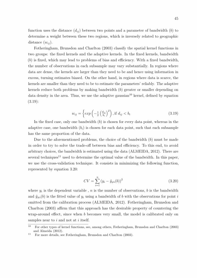
45

function uses the distance (dij) between two points and a parameter of bandwidth (b) todetermine a weight between these two regions, which is inversely related to geographicdistance (wij).

Fotheringham, Brunsdon and Charlton (2003) classify the spatial kernel functions intwo groups: the fixed kernels and the adaptive kernels. In the fixed kernels, bandwidth(b) is fixed, which may lead to problems of bias and efficiency. With a fixed bandwidth,the number of observations in each subsample may vary substantially. In regions wheredata are dense, the kernels are larger than they need to be and hence using information inexcess, turning estimates biased. On the other hand, in regions where data is scarce, thekernels are smaller than they need to be to estimate the parameters’ reliably. The adaptivekernels reduce both problems by making bandwidth (b) greater or smaller depending ondata density in the area. Thus, we use the adaptive gaussian10 kernel, defined by equation(3.19):

wij ={exp

(−1

2

(dij

bi

)2), if dij < bi (3.19)

In the fixed case, only one bandwidth (b) is chosen for every data point, whereas in theadaptive case, one bandwidth (bi) is chosen for each data point, such that each subsamplehas the same proportion of the data.

Due to the aforementioned problems, the choice of the bandwidth (b) must be madein order to try to solve the trade-off between bias and efficiency. To this end, to avoidarbitrary choices, the bandwidth is estimated using the data (ALMEIDA, 2012). There areseveral techniques11 used to determine the optimal value of the bandwidth. In this paper,we use the cross-validation technique. It consists in minimizing the following function,represented by equation 3.20:

CV =n∑i=1

(yi − y6=i(b))2 (3.20)

where yi is the dependent variable , n is the number of observations, b is the bandwidthand y 6=i(b) is the fitted value of yi using a bandwidth of b with the observations for point iomitted from the calibration process (ALMEIDA, 2012). Fotheringham, Brunsdon andCharlton (2003) affirm that this approach has the desirable property of countering thewrap-around effect, since when b becomes very small, the model is calibrated only onsamples near to i and not at i itself.10 For other types of kernel functions, see, among others, Fotheringham, Brunsdon and Charlton (2003)

and Almeida (2012).11 For more details, see Fotheringham, Brunsdon and Charlton (2003).

46

After obtaining these weights generated by the kernel function, it is possible to get thelocal spatial weighting diagonal matrix:

W (ui, vi) =

wi1 0 · · · 00 wi2 · · · 0... ... . . . ...0 0 · · · win

(3.21)

where win is the weight attributed to point n in the model calibration in regression pointi, obtained by means of spatial kernel function. Thus, from the model showed in equation(3.16), the local model can be specified by the following weighted maximum likelihoodfunction, represented by equation (3.22):

logL =n∑i=1

W (ui, vi)log[Φ(log(tu+1i)− µ

σ

)− Φ

(log(tui)− µ

σ

)](3.22)

From the equation above, are estimated parameter sets for each n points. Next sectionpresents results of the estimation for both global and local models.

3.5 RESULTS

3.5.1 Results from the Global Model

Table 3.6 shows the results of the estimation of the global model represented by equation(3.16). All parameters are statistically significant. The sign of estimates indicate theeffect on willingness to pay. All variables, except Age, show positive signs. The negativesign of variable Age indicates that older people tend to pay less to reduce crime thanyoung people, indicating that older people have a greater feeling of security than youngpeople. As to variables Gender and Education, the positive sign indicates that men andmore educated people tend to pay more to reduce the risk of being robbed. Finally, as tovariables of perception and experience of victimization (variable Perception of patrollingis measured in decreasing order), the lower the perception of patrolling, the greater thewillingness to pay to reduce the number of robberies, and people who were Victims ofrobbery tend to pay more to prevent such experience again.Variable I(Subject Prob. * Income) deserves special attention. The positive sign of thisvariable shows that the higher the income and the subjective probability of being robbed,the higher the willingness to pay to reduce the risk of being robbed. On the other hand,when this variable is multiplied by θ, we have the fraction, in average, of the incomerobbed in each robbery. This value is equal to approximately 0.0415. So, in each robbery,approximately 4,15% of the income is robbed. Multiplying this value by the averageincome, we have a value of R$ 61,38 per robbery.

In table 3.7, the values of estimated WTP, as defined by equation 3.17, are presented.

47

Table 3.6 – Estimates - Parametric Maximum Likelihood

Variable Estimate Stand. Dev. t p-value(Intercept) 2.3949 0.1024 23.3750 0.0000I(Subject Prob. * Income) 0.0002 0.0000 4.7072 0.0000Gender 0.1897 0.0477 3.9738 0.0000Age -0.0034 0.0016 -2.0946 0.0362Education 0.0466 0.0160 2.9058 0.0036Perception of patrolling 0.0520 0.0196 2.6559 0.0079Victim of robbery 0.0926 0.0550 1.6818 0.0926σ 0.7299 0.0167 43.6735 0.0000log-likelihood = -1851.53Newton-Raphson maximization, 4 interationsSource: Elaborated by the authors

Table 3.7 – Results of WTP(R$) from the global parametric model

Variable Estimate Stand. Dev. Inter. Conf.Mean 23.35 6.12 22.98 - 23.72Median 16.21 4.25 15.95 - 16.47Source: Elaborated by the authors

The average WTP estimated from the global model is equal to R$ 23.35 per month/household,a value R$ 5.91, which is higher than the estimated value of the nonparametric form,which was only R$ 17.44. Thus, if the government decided to implement a monthly taxabout this value, it would be possible to raise, per year, R$ 280.20 per household, whichwould generate an average tax revenue of about R$ 198.92 million per year, equivalentto approximately 20.63% of the amount spent on public security in the state of Ceará in201112. Assuming a worst case scenario, using the median WTP value of R$ 16.21 permonth/household as a benchmark, we have a value of R$ 194.52 per year/household. Inthis case, the annual tax revenue in Fortaleza would be approximately R$ 138.09 million,equivalent to 14.32% of spending on public security in 2011.

Now, considering the damage of robberies to society, in the first scenario, where theWTP was estimated in R$ 23.35, we got an implicit value of a statistical robbery ofapproximately R$ 11,969 per robbery avoided. Considering the second scenario, wherewe assumed the WTP median value equal to R$ 16.21, the value of a statistical robberywas estimated approximately equal to R$ 8,310 per crime avoided. Next section presentsresults from the local model.12 According to Pública (2012), the amount spent on public security in the state of Ceará in the year of

2011 was R$ 964,095,556.61.

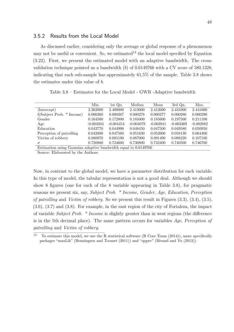
48

3.5.2 Results from the Local Model

As discussed earlier, considering only the average or global response of a phenomenonmay not be useful or convenient. So, we estimated13 the local model specified by Equation(3.22). First, we present the estimated model with an adaptive bandwidth. The cross-validation technique pointed us a bandwidth (b) of 0.6149766 with a CV score of 580.1328,indicating that each sub-sample has approximately 61,5% of the sample. Table 3.8 showsthe estimates under this value of b.

Table 3.8 – Estimates for the Local Model - GWR -Adaptive bandwidth

Min. 1st Qu. Median Mean 3rd Qu. Max.(Intercept) 2.362000 2.400000 2.413000 2.412000 2.431000 2.441000I(Subject Prob. * Income) 0.000260 0.000267 0.000278 0.000277 0.000286 0.000290Gender 0.164500 0.172800 0.183400 0.185600 0.197500 0.211100Age -0.004934 -0.004454 -0.004079 -0.003941 -0.003369 -0.002882Education 0.043770 0.044990 0.048450 0.047500 0.049580 0.050950Perception of patrolling 0.042800 0.047560 0.051630 0.052600 0.058130 0.064400Victim of robbery 0.080970 0.085190 0.087000 0.091490 0.098220 0.107100σ 0.720800 0.724600 0.730800 0.732400 0.740500 0.746700Estimation using Gaussian adaptive bandwidth equal to 0.6149766Source: Elaborated by the Authors

Now, in contrast to the global model, we have a parameter distribution for each variable.In this type of model, the tabular representation is not a good deal. Although we shouldshow 8 figures (one for each of the 8 variable appearing in Table 3.8), for pragmaticreasons we present six, say, Subject Prob. * Income, Gender, Age, Education, Perceptionof patrolling and Victim of robbery. So we present this result in Figures (3.3), (3.4), (3.5),(3.6), (3.7) and (3.8). For example, in the east region of the city of Fortaleza, the impactof variable Subject Prob. * Income is slightly greater than in west regions (the differenceis in the 5th decimal place). The same pattern occurs for variables Age, Perception ofpatrolling and Victim of robbery.13 To estimate this model, we use the R statistical software (R Core Team (2014)), more specifically

packages “maxLik” (Henningsen and Toomet (2011)) and “spgwr” (Bivand and Yu (2013)).

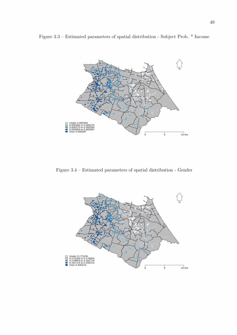
49

Figure 3.3 – Estimated parameters of spatial distribution - Subject Prob. * Income

●

●

●

●

●

●●

●●

●

●

●

●

●

●● ●●

●

●

●

●

●●

●

●

●●

●

●

●

●

●●

●

●

●

●

●●

●●●●

●●

●

●

●●

●

●

●

●

● ●●

●

●●●●●●

●●

●●

●

●

●●

●●

●

●

●●●

●

●

●●

●

●●●●

●

●

●

●

●

●

●●

●●

●●

●

●

●

●

●

●

●●

●●

●

●

●

●

●●●

●

●

●●●●

●

●●●●●●

●

●

●●

●

●

●

●

●

●

●

●●●

●●●

●●

●●

●●

●●●

●

●

●

●

●●

●

●●●

●

●

●

●

●

●●

●●

●

●

●

●

●

●

●

●●

●

●●●

●●

●

●

●

●

●

●

●

●● ●

●

●

●

●

●●●

●

●

●

●

●

●

●●●

●●

●●●

●●

●

●

●

●

●

●●

●●

●

●

●

●●

●●●

●●● ●

●

●

●

●

●

●●

●

●

●●●

●

● ●

●

●

●●

●

●●●

●

●

●

●●●

●

●

●

●●

●

●

●

●

●●●

●

●

●

●●

●

●

●●

●●●●

●●

●

●

●●

●●

●●

●

●

●●

●

●●

●●

●

●●●●

●

●

●●

●●

●●●●●

●

●

●

●●

●

●

●

●●

●

●

●

●●

●

●

●

●

●

●

●

●

●●● ●

●

●● ●

●

●

●

● ●

●●

●

●

●

●●●

●

●●

●●

●●

●●

●

●

●

●

●●

●

●●●●

●●●

●

●

●

●●●

●●

●

●

●

●

●●

●●●●

●●●

●

●

●●●●

●●●

●

●

●

●

●

●

●

●●●●

●●●

●

●●●

●●

●●●

●

●

●

●●

●●●

●●●

●

●

●

●

●●●

●

●●●

●●

●

●●●● ●●

●●

●●

●

●

●●● ●

●

●

●

●

●

●

●

●●●

●●●

●●●●

●

●●●●●●

●●

●

●

●

●

●●● ●●●●

●●

●

●●

●

●

●

●●●●●

●

●

●●

●

●●●●

●●

●

●

●

●

●●●

●

●

● ●

●

●●

●●●●●

●

●

●

●

●

●

●

●●

●●●

●●

●

●●●

●●●

●

●●●

●

●

●

●●●●

●●●●●

●

●

●

●●●●●●

●●

●

●●

●

●●●●●

●●

●

●●

●●

●

● ●●●

●

●

●●●●

●

● ●●●

●

● ●

●

●

●●●

●

●●

●

●●

●●

●●●

●

●●

●

●●

●●

●

●●●●●

●

● ●

●●●

●●

●●●

●

●●●

●●

●

●●

●●

●

●

●

●

●

●●

●

●

●

●●

●

●

●●

●●●

●

●●

●

●●

●

●

●

●

●

●

●●●

●

●

●

●

●●●

●

●

●●●

●●

●●● ●

●

●●●

●

●

●●

●●

●

●

●●●●●

●●●●●

●

●

●

●●●

●●

●

●

●

●

●

●●●●

●

●

●●●

●

●●●

●

●●

●

●

●●

●

●

●●

●●

●●

●●●

●

●

●

●●●●●

●●●●

●

●

●

●

●●

●● ●

●

●

●

●●●

●●●●●●●

●

●

●

●

●

●

●●

●

●

●

●

●

●

●

●

●●●

●●

●

●

●●

●●

●

●

●

●●

●

●

●●

●

●●

●

●●

●

●

●

●

●

●

●●● ●

●●●

●

●

●

●●●

●●

●

●

●

●

●

●

●

●

●●●

●

●

●

●

●

●

●

●●●

●●●

●

●

●

●

●

●●

● ●

●

●

●●

●

●●

●

●●

●●

●

●●

●

●●

●

●

●

●●

●

●

●

●

●

●●

●●●●●●●

●

●●

●●●

●

●●●

●

●

●

●

●●

●●●

●●●

●

●●

●

●

●●●

●●

●

●

●

●

●

●

●●●

●●

●

Under 0.0002650.000265 to 0.0002750.000275 to 0.0002830.000283 to 0.000287Over 0.000287

0 5 10 km

N

Figure 3.4 – Estimated parameters of spatial distribution - Gender

●

●

●

●

●

●●

●●

●

●

●

●

●

●● ●●

●

●

●

●

●●

●

●

●●

●

●

●

●

●●

●

●

●

●

●●

●●●●

●●

●

●

●●

●

●

●

●

● ●●

●

●●●●●●

●●

●●

●

●

●●

●●

●

●

●●●

●

●

●●

●

●●●●

●

●

●

●

●

●

●●

●●

●●

●

●

●

●

●

●

●●

●●

●

●

●

●

●●●

●

●

●●●●

●

●●●●●●

●

●

●●

●

●

●

●

●

●

●

●●●

●●●

●●

●●

●●

●●●

●

●

●

●

●●

●

●●●

●

●

●

●

●

●●

●●

●

●

●

●

●

●

●

●●

●

●●●

●●

●

●

●

●

●

●

●

●● ●

●

●

●

●

●●●

●

●

●

●

●

●

●●●

●●

●●●

●●

●

●

●

●

●

●●

●●

●

●

●

●●

●●●

●●● ●

●

●

●

●

●

●●

●

●

●●●

●

● ●

●

●

●●

●

●●●

●

●

●

●●●

●

●

●

●●

●

●

●

●

●●●

●

●

●

●●

●

●

●●

●●●●

●●

●

●

●●

●●

●●

●

●

●●

●

●●

●●

●

●●●●

●

●

●●

●●

●●●●●

●

●

●

●●

●

●

●

●●

●

●

●

●●

●

●

●

●

●

●

●

●

●●● ●

●

●● ●

●

●

●

● ●

●●

●

●

●

●●●

●

●●

●●

●●

●●

●

●

●

●

●●

●

●●●●

●●●

●

●

●

●●●

●●

●

●

●

●

●●

●●●●

●●●

●

●

●●●●

●●●

●

●

●

●

●

●

●

●●●●

●●●

●

●●●

●●

●●●

●

●

●

●●

●●●

●●●

●

●

●

●

●●●

●

●●●

●●

●

●●●● ●●

●●

●●

●

●

●●● ●

●

●

●

●

●

●

●

●●●

●●●

●●●●

●

●●●●●●

●●

●

●

●

●

●●● ●●●●

●●

●

●●

●

●

●

●●●●●

●

●

●●

●

●●●●

●●

●

●

●

●

●●●

●

●

● ●

●

●●

●●●●●

●

●

●

●

●

●

●

●●

●●●

●●

●

●●●

●●●

●

●●●

●

●

●

●●●●

●●●●●

●

●

●

●●●●●●

●●

●

●●

●

●●●●●

●●

●

●●

●●

●

● ●●●

●

●

●●●●

●

● ●●●

●

● ●

●

●

●●●

●

●●

●

●●

●●

●●●

●

●●

●

●●

●●

●

●●●●●

●

● ●

●●●

●●

●●●

●

●●●

●●

●

●●

●●

●

●

●

●

●

●●

●

●

●

●●

●

●

●●

●●●

●

●●

●

●●

●

●

●

●

●

●

●●●

●

●

●

●

●●●

●

●

●●●

●●

●●● ●

●

●●●

●

●

●●

●●

●

●

●●●●●

●●●●●

●

●

●

●●●

●●

●

●

●

●

●

●●●●

●

●

●●●

●

●●●

●

●●

●

●

●●

●

●

●●

●●

●●

●●●

●

●

●

●●●●●

●●●●

●

●

●

●

●●

●● ●

●

●

●

●●●

●●●●●●●

●

●

●

●

●

●

●●

●

●

●

●

●

●

●

●

●●●

●●

●

●

●●

●●

●

●

●

●●

●

●

●●

●

●●

●

●●

●

●

●

●

●

●

●●● ●

●●●

●

●

●

●●●

●●

●

●

●

●

●

●

●

●

●●●

●

●

●

●

●

●

●

●●●

●●●

●

●

●

●

●

●●

● ●

●

●

●●

●

●●

●

●●

●●

●

●●

●

●●

●

●

●

●●

●

●

●

●

●

●●

●●●●●●●

●

●●

●●●

●

●●●

●

●

●

●

●●

●●●

●●●

●

●●

●

●

●●●

●●

●

●

●

●

●

●

●●●

●●

●


0 5 10 km

N

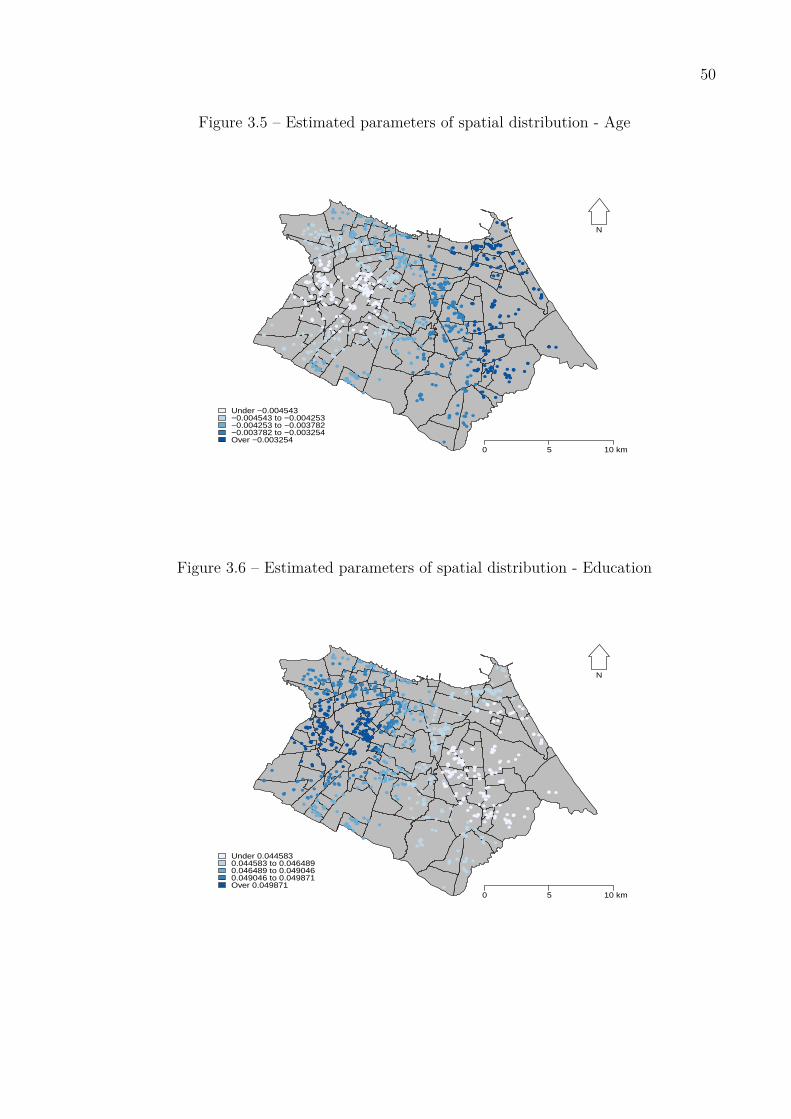
50

Figure 3.5 – Estimated parameters of spatial distribution - Age

●

●

●

●

●

●●

●●

●

●

●

●

●

●● ●●

●

●

●

●

●●

●

●

●●

●

●

●

●

●●

●

●

●

●

●●

●●●●

●●

●

●

●●

●

●

●

●

● ●●

●

●●●●●●

●●

●●

●

●

●●

●●

●

●

●●●

●

●

●●

●

●●●●

●

●

●

●

●

●

●●

●●

●●

●

●

●

●

●

●

●●

●●

●

●

●

●

●●●

●

●

●●●●

●

●●●●●●

●

●

●●

●

●

●

●

●

●

●

●●●

●●●

●●

●●

●●

●●●

●

●

●

●

●●

●

●●●

●

●

●

●

●

●●

●●

●

●

●

●

●

●

●

●●

●

●●●

●●

●

●

●

●

●

●

●

●● ●

●

●

●

●

●●●

●

●

●

●

●

●

●●●

●●

●●●

●●

●

●

●

●

●

●●

●●

●

●

●

●●

●●●

●●● ●

●

●

●

●

●

●●

●

●

●●●

●

● ●

●

●

●●

●

●●●

●

●

●

●●●

●

●

●

●●

●

●

●

●

●●●

●

●

●

●●

●

●

●●

●●●●

●●

●

●

●●

●●

●●

●

●

●●

●

●●

●●

●

●●●●

●

●

●●

●●

●●●●●

●

●

●

●●

●

●

●

●●

●

●

●

●●

●

●

●

●

●

●

●

●

●●● ●

●

●● ●

●

●

●

● ●

●●

●

●

●

●●●

●

●●

●●

●●

●●

●

●

●

●

●●

●

●●●●

●●●

●

●

●

●●●

●●

●

●

●

●

●●

●●●●

●●●

●

●

●●●●

●●●

●

●

●

●

●

●

●

●●●●

●●●

●

●●●

●●

●●●

●

●

●

●●

●●●

●●●

●

●

●

●

●●●

●

●●●

●●

●

●●●● ●●

●●

●●

●

●

●●● ●

●

●

●

●

●

●

●

●●●

●●●

●●●●

●

●●●●●●

●●

●

●

●

●

●●● ●●●●

●●

●

●●

●

●

●

●●●●●

●

●

●●

●

●●●●

●●

●

●

●

●

●●●

●

●

● ●

●

●●

●●●●●

●

●

●

●

●

●

●

●●

●●●

●●

●

●●●

●●●

●

●●●

●

●

●

●●●●

●●●●●

●

●

●

●●●●●●

●●

●

●●

●

●●●●●

●●

●

●●

●●

●

● ●●●

●

●

●●●●

●

● ●●●

●

● ●

●

●

●●●

●

●●

●

●●

●●

●●●

●

●●

●

●●

●●

●

●●●●●

●

● ●

●●●

●●

●●●

●

●●●

●●

●

●●

●●

●

●

●

●

●

●●

●

●

●

●●

●

●

●●

●●●

●

●●

●

●●

●

●

●

●

●

●

●●●

●

●

●

●

●●●

●

●

●●●

●●

●●● ●

●

●●●

●

●

●●

●●

●

●

●●●●●

●●●●●

●

●

●

●●●

●●

●

●

●

●

●

●●●●

●

●

●●●

●

●●●

●

●●

●

●

●●

●

●

●●

●●

●●

●●●

●

●

●

●●●●●

●●●●

●

●

●

●

●●

●● ●

●

●

●

●●●

●●●●●●●

●

●

●

●

●

●

●●

●

●

●

●

●

●

●

●

●●●

●●

●

●

●●

●●

●

●

●

●●

●

●

●●

●

●●

●

●●

●

●

●

●

●

●

●●● ●

●●●

●

●

●

●●●

●●

●

●

●

●

●

●

●

●

●●●

●

●

●

●

●

●

●

●●●

●●●

●

●

●

●

●

●●

● ●

●

●

●●

●

●●

●

●●

●●

●

●●

●

●●

●

●

●

●●

●

●

●

●

●

●●

●●●●●●●

●

●●

●●●

●

●●●

●

●

●

●

●●

●●●

●●●

●

●●

●

●

●●●

●●

●

●

●

●

●

●

●●●

●●

●

Under −0.004543−0.004543 to −0.004253−0.004253 to −0.003782−0.003782 to −0.003254Over −0.003254

0 5 10 km

N

Figure 3.6 – Estimated parameters of spatial distribution - Education

●

●

●

●

●

●●

●●

●

●

●

●

●

●● ●●

●

●

●

●

●●

●

●

●●

●

●

●

●

●●

●

●

●

●

●●

●●●●

●●

●

●

●●

●

●

●

●

● ●●

●

●●●●●●

●●

●●

●

●

●●

●●

●

●

●●●

●

●

●●

●

●●●●

●

●

●

●

●

●

●●

●●

●●

●

●

●

●

●

●

●●

●●

●

●

●

●

●●●

●

●

●●●●

●

●●●●●●

●

●

●●

●

●

●

●

●

●

●

●●●

●●●

●●

●●

●●

●●●

●

●

●

●

●●

●

●●●

●

●

●

●

●

●●

●●

●

●

●

●

●

●

●

●●

●

●●●

●●

●

●

●

●

●

●

●

●● ●

●

●

●

●

●●●

●

●

●

●

●

●

●●●

●●

●●●

●●

●

●

●

●

●

●●

●●

●

●

●

●●

●●●

●●● ●

●

●

●

●

●

●●

●

●

●●●

●

● ●

●

●

●●

●

●●●

●

●

●

●●●

●

●

●

●●

●

●

●

●

●●●

●

●

●

●●

●

●

●●

●●●●

●●

●

●

●●

●●

●●

●

●

●●

●

●●

●●

●

●●●●

●

●

●●

●●

●●●●●

●

●

●

●●

●

●

●

●●

●

●

●

●●

●

●

●

●

●

●

●

●

●●● ●

●

●● ●

●

●

●

● ●

●●

●

●

●

●●●

●

●●

●●

●●

●●

●

●

●

●

●●

●

●●●●

●●●

●

●

●

●●●

●●

●

●

●

●

●●

●●●●

●●●

●

●

●●●●

●●●

●

●

●

●

●

●

●

●●●●

●●●

●

●●●

●●

●●●

●

●

●

●●

●●●

●●●

●

●

●

●

●●●

●

●●●

●●

●

●●●● ●●

●●

●●

●

●

●●● ●

●

●

●

●

●

●

●

●●●

●●●

●●●●

●

●●●●●●

●●

●

●

●

●

●●● ●●●●

●●

●

●●

●

●

●

●●●●●

●

●

●●

●

●●●●

●●

●

●

●

●

●●●

●

●

● ●

●

●●

●●●●●

●

●

●

●

●

●

●

●●

●●●

●●

●

●●●

●●●

●

●●●

●

●

●

●●●●

●●●●●

●

●

●

●●●●●●

●●

●

●●

●

●●●●●

●●

●

●●

●●

●

● ●●●

●

●

●●●●

●

● ●●●

●

● ●

●

●

●●●

●

●●

●

●●

●●

●●●

●

●●

●

●●

●●

●

●●●●●

●

● ●

●●●

●●

●●●

●

●●●

●●

●

●●

●●

●

●

●

●

●

●●

●

●

●

●●

●

●

●●

●●●

●

●●

●

●●

●

●

●

●

●

●

●●●

●

●

●

●

●●●

●

●

●●●

●●

●●● ●

●

●●●

●

●

●●

●●

●

●

●●●●●

●●●●●

●

●

●

●●●

●●

●

●

●

●

●

●●●●

●

●

●●●

●

●●●

●

●●

●

●

●●

●

●

●●

●●

●●

●●●

●

●

●

●●●●●

●●●●

●

●

●

●

●●

●● ●

●

●

●

●●●

●●●●●●●

●

●

●

●

●

●

●●

●

●

●

●

●

●

●

●

●●●

●●

●

●

●●

●●

●

●

●

●●

●

●

●●

●

●●

●

●●

●

●

●

●

●

●

●●● ●

●●●

●

●

●

●●●

●●

●

●

●

●

●

●

●

●

●●●

●

●

●

●

●

●

●

●●●

●●●

●

●

●

●

●

●●

● ●

●

●

●●

●

●●

●

●●

●●

●

●●

●

●●

●

●

●

●●

●

●

●

●

●

●●

●●●●●●●

●

●●

●●●

●

●●●

●

●

●

●

●●

●●●

●●●

●

●●

●

●

●●●

●●

●

●

●

●

●

●

●●●

●●

●


0 5 10 km

N

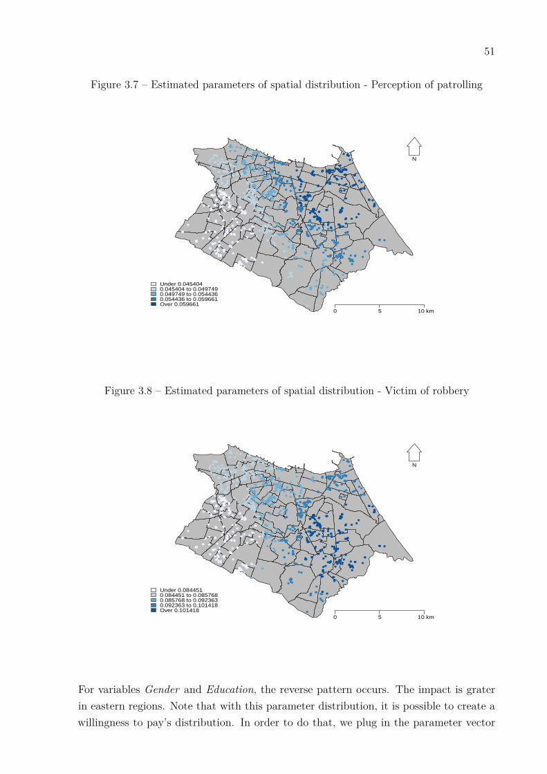
51

Figure 3.7 – Estimated parameters of spatial distribution - Perception of patrolling

●

●

●

●

●

●●

●●

●

●

●

●

●

●● ●●

●

●

●

●

●●

●

●

●●

●

●

●

●

●●

●

●

●

●

●●

●●●●

●●

●

●

●●

●

●

●

●

● ●●

●

●●●●●●

●●

●●

●

●

●●

●●

●

●

●●●

●

●

●●

●

●●●●

●

●

●

●

●

●

●●

●●

●●

●

●

●

●

●

●

●●

●●

●

●

●

●

●●●

●

●

●●●●

●

●●●●●●

●

●

●●

●

●

●

●

●

●

●

●●●

●●●

●●

●●

●●

●●●

●

●

●

●

●●

●

●●●

●

●

●

●

●

●●

●●

●

●

●

●

●

●

●

●●

●

●●●

●●

●

●

●

●

●

●

●

●● ●

●

●

●

●

●●●

●

●

●

●

●

●

●●●

●●

●●●

●●

●

●

●

●

●

●●

●●

●

●

●

●●

●●●

●●● ●

●

●

●

●

●

●●

●

●

●●●

●

● ●

●

●

●●

●

●●●

●

●

●

●●●

●

●

●

●●

●

●

●

●

●●●

●

●

●

●●

●

●

●●

●●●●

●●

●

●

●●

●●

●●

●

●

●●

●

●●

●●

●

●●●●

●

●

●●

●●

●●●●●

●

●

●

●●

●

●

●

●●

●

●

●

●●

●

●

●

●

●

●

●

●

●●● ●

●

●● ●

●

●

●

● ●

●●

●

●

●

●●●

●

●●

●●

●●

●●

●

●

●

●

●●

●

●●●●

●●●

●

●

●

●●●

●●

●

●

●

●

●●

●●●●

●●●

●

●

●●●●

●●●

●

●

●

●

●

●

●

●●●●

●●●

●

●●●

●●

●●●

●

●

●

●●

●●●

●●●

●

●

●

●

●●●

●

●●●

●●

●

●●●● ●●

●●

●●

●

●

●●● ●

●

●

●

●

●

●

●

●●●

●●●

●●●●

●

●●●●●●

●●

●

●

●

●

●●● ●●●●

●●

●

●●

●

●

●

●●●●●

●

●

●●

●

●●●●

●●

●

●

●

●

●●●

●

●

● ●

●

●●

●●●●●

●

●

●

●

●

●

●

●●

●●●

●●

●

●●●

●●●

●

●●●

●

●

●

●●●●

●●●●●

●

●

●

●●●●●●

●●

●

●●

●

●●●●●

●●

●

●●

●●

●

● ●●●

●

●

●●●●

●

● ●●●

●

● ●

●

●

●●●

●

●●

●

●●

●●

●●●

●

●●

●

●●

●●

●

●●●●●

●

● ●

●●●

●●

●●●

●

●●●

●●

●

●●

●●

●

●

●

●

●

●●

●

●

●

●●

●

●

●●

●●●

●

●●

●

●●

●

●

●

●

●

●

●●●

●

●

●

●

●●●

●

●

●●●

●●

●●● ●

●

●●●

●

●

●●

●●

●

●

●●●●●

●●●●●

●

●

●

●●●

●●

●

●

●

●

●

●●●●

●

●

●●●

●

●●●

●

●●

●

●

●●

●

●

●●

●●

●●

●●●

●

●

●

●●●●●

●●●●

●

●

●

●

●●

●● ●

●

●

●

●●●

●●●●●●●

●

●

●

●

●

●

●●

●

●

●

●

●

●

●

●

●●●

●●

●

●

●●

●●

●

●

●

●●

●

●

●●

●

●●

●

●●

●

●

●

●

●

●

●●● ●

●●●

●

●

●

●●●

●●

●

●

●

●

●

●

●

●

●●●

●

●

●

●

●

●

●

●●●

●●●

●

●

●

●

●

●●

● ●

●

●

●●

●

●●

●

●●

●●

●

●●

●

●●

●

●

●

●●

●

●

●

●

●

●●

●●●●●●●

●

●●

●●●

●

●●●

●

●

●

●

●●

●●●

●●●

●

●●

●

●

●●●

●●

●

●

●

●

●

●

●●●

●●

●


0 5 10 km

N

Figure 3.8 – Estimated parameters of spatial distribution - Victim of robbery

●

●

●

●

●

●●

●●

●

●

●

●

●

●● ●●

●

●

●

●

●●

●

●

●●

●

●

●

●

●●

●

●

●

●

●●

●●●●

●●

●

●

●●

●

●

●

●

● ●●

●

●●●●●●

●●

●●

●

●

●●

●●

●

●

●●●

●

●

●●

●

●●●●

●

●

●

●

●

●

●●

●●

●●

●

●

●

●

●

●

●●

●●

●

●

●

●

●●●

●

●

●●●●

●

●●●●●●

●

●

●●

●

●

●

●

●

●

●

●●●

●●●

●●

●●

●●

●●●

●

●

●

●

●●

●

●●●

●

●

●

●

●

●●

●●

●

●

●

●

●

●

●

●●

●

●●●

●●

●

●

●

●

●

●

●

●● ●

●

●

●

●

●●●

●

●

●

●

●

●

●●●

●●

●●●

●●

●

●

●

●

●

●●

●●

●

●

●

●●

●●●

●●● ●

●

●

●

●

●

●●

●

●

●●●

●

● ●

●

●

●●

●

●●●

●

●

●

●●●

●

●

●

●●

●

●

●

●

●●●

●

●

●

●●

●

●

●●

●●●●

●●

●

●

●●

●●

●●

●

●

●●

●

●●

●●

●

●●●●

●

●

●●

●●

●●●●●

●

●

●

●●

●

●

●

●●

●

●

●

●●

●

●

●

●

●

●

●

●

●●● ●

●

●● ●

●

●

●

● ●

●●

●

●

●

●●●

●

●●

●●

●●

●●

●

●

●

●

●●

●

●●●●

●●●

●

●

●

●●●

●●

●

●

●

●

●●

●●●●

●●●

●

●

●●●●

●●●

●

●

●

●

●

●

●

●●●●

●●●

●

●●●

●●

●●●

●

●

●

●●

●●●

●●●

●

●

●

●

●●●

●

●●●

●●

●

●●●● ●●

●●

●●

●

●

●●● ●

●

●

●

●

●

●

●

●●●

●●●

●●●●

●

●●●●●●

●●

●

●

●

●

●●● ●●●●

●●

●

●●

●

●

●

●●●●●

●

●

●●

●

●●●●

●●

●

●

●

●

●●●

●

●

● ●

●

●●

●●●●●

●

●

●

●

●

●

●

●●

●●●

●●

●

●●●

●●●

●

●●●

●

●

●

●●●●

●●●●●

●

●

●

●●●●●●

●●

●

●●

●

●●●●●

●●

●

●●

●●

●

● ●●●

●

●

●●●●

●

● ●●●

●

● ●

●

●

●●●

●

●●

●

●●

●●

●●●

●

●●

●

●●

●●

●

●●●●●

●

● ●

●●●

●●

●●●

●

●●●

●●

●

●●

●●

●

●

●

●

●

●●

●

●

●

●●

●

●

●●

●●●

●

●●

●

●●

●

●

●

●

●

●

●●●

●

●

●

●

●●●

●

●

●●●

●●

●●● ●

●

●●●

●

●

●●

●●

●

●

●●●●●

●●●●●

●

●

●

●●●

●●

●

●

●

●

●

●●●●

●

●

●●●

●

●●●

●

●●

●

●

●●

●

●

●●

●●

●●

●●●

●

●

●

●●●●●

●●●●

●

●

●

●

●●

●● ●

●

●

●

●●●

●●●●●●●

●

●

●

●

●

●

●●

●

●

●

●

●

●

●

●

●●●

●●

●

●

●●

●●

●

●

●

●●

●

●

●●

●

●●

●

●●

●

●

●

●

●

●

●●● ●

●●●

●

●

●

●●●

●●

●

●

●

●

●

●

●

●

●●●

●

●

●

●

●

●

●

●●●

●●●

●

●

●

●

●

●●

● ●

●

●

●●

●

●●

●

●●

●●

●

●●

●

●●

●

●

●

●●

●

●

●

●

●

●●

●●●●●●●

●

●●

●●●

●

●●●

●

●

●

●

●●

●●●

●●●

●

●●

●

●

●●●

●●

●

●

●

●

●

●

●●●

●●

●


0 5 10 km

N

For variables Gender and Education, the reverse pattern occurs. The impact is graterin eastern regions. Note that with this parameter distribution, it is possible to create awillingness to pay’s distribution. In order to do that, we plug in the parameter vector

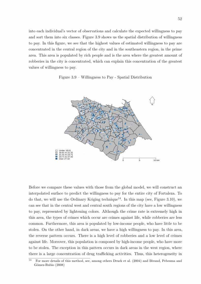
52

into each individual’s vector of observations and calculate the expected willingness to payand sort them into six classes. Figure 3.9 shows us the spatial distribution of willingnessto pay. In this figure, we see that the highest values of estimated willingness to pay areconcentrated in the central region of the city and in the southeastern region, in the primearea. This area is populated by rich people and is the area where the greatest amount ofrobberies in the city is concentrated, which can explain this concentration of the greatestvalues of willingness to pay.

Figure 3.9 – Willingness to Pay - Spatial Distribution

●

●

●

●

●

●●

●●

●

●

●

●

●

●● ●●

●

●

●

●

●●

●

●

●●

●

●

●

●

●●

●

●

●

●

●●

●●●●

●●

●

●

●●

●

●

●

●

● ●●

●

●●●●●●

●●

●●

●

●

●●

●●

●

●

●●●

●

●

●●

●

●●●●

●

●

●

●

●

●

●●

●●

●●

●

●

●

●

●

●

●●

●●

●

●

●

●

●●●

●

●

●●●●

●

●●●●●●

●

●

●●

●

●

●

●

●

●

●

●●●

●●●

●●

●●

●●

●●●

●

●

●

●

●●

●

●●●

●

●

●

●

●

●●

●●

●

●

●

●

●

●

●

●●

●

●●●

●●

●

●

●

●

●

●

●

●● ●

●

●

●

●

●●●

●

●

●

●

●

●

●●●

●●

●●●

●●

●

●

●

●

●

●●

●●

●

●

●

●●

●●●

●●● ●

●

●

●

●

●

●●

●

●

●●●

●

● ●

●

●

●●

●

●●●

●

●

●

●●●

●

●

●

●●

●

●

●

●

●●●

●

●

●

●●

●

●

●●

●●●●

●●

●

●

●●

●●

●●

●

●

●●

●

●●

●●

●

●●●●

●

●

●●

●●

●●●●●

●

●

●

●●

●

●

●

●●

●

●

●

●●

●

●

●

●

●

●

●

●

●

●●● ●

●

●● ●

●

●

●

● ●

●●

●

●

●

●●●

●

●●

●●

●●

●●

●

●

●

●

●●

●

●●●●

●●●

●

●

●

●●●

●●

●

●

●

●

●●

●●●●

●●●

●

●

●●●●

●●●

●

●

●

●

●

●

●

●●●●

●●●

●

●●●

●●

●●●

●

●

●

●●

●●●

●●●

●

●

●

●

●●●

●

●●●

●●

●

●●●● ●●

●●

●●

●

●

●●● ●

●

●

●

●

●

●

●

●●●

●●●

●●●●

●

●●●●●●

●●

●

●

●

●

●●● ●●●●

●●

●

●●

●

●

●

●●●●●

●

●

●●

●

●●●●

●●

●

●

●

●

●●●

●

●

● ●

●

●●

●●●●●

●

●

●

●

●

●

●

●●

●●●

●●

●

●●●

●●●

●

●●●

●

●

●

●●●●

●●●●●

●

●

●

●●●●●●

●●

●

●●

●

●●●●●

●●

●

●●

●●

●

● ●●●

●

●

●●●●

●

●

● ●●●

●

● ●

●

●

●●●

●

●●

●

●●

●●

●●●

●

●●

●

●●

●●

●

●●●●●

●

● ●

●●●

●●

●●●

●

●●●

●●

●

●●

●●

●

●

●

●

●●

●

●●

●●

●

●

●

●●

●

●

●●

●●●

●

●●

●

●●

●

●

●

●

●

●

●●●

●

●

●

●

●●●

●

●

●●●

●●

●●● ●

●

●●●

●

●

●●

●●

●

●

●●●●●

●●●●●

●

●

●

●●●

●●

●

●

●

●

●

●●●●

●

●

●●●

●

●●●

●

●●

●

●

●●

●

●

●●

●●

●●

●●●

●

●

●

●●●●●

●●●●

●

●

●

●

●●

●● ●

●

●

●

●●●

●●●●●●●

●

●

●

●

●

●

●●

●

●

●

●

●

●

●

●

●●●

●●

●

●

●●

●●

●

●

●

●●

●

●

●●

●

●●

●

●●

●

●

●

●

●

●

●●● ●

●●●

●

●

●

●●●

●●

●

●

●

●

●

●

●

●

●●●

●

●

●

●

●

●

●

●●●

●●●

●

●

●

●

●

●●

● ●

●

●

●●

●

●●

●

●●

●●

●

●●

●

●●

●

●

●

●●

●

●

●

●

●

●●

●●●●●●●

●

●●

●●●

●

●●●

●

●

●

●

●●

●●●

●●●

●

●●

●

●

●●●

●●

●

●

●

●

●

●

●●●

●●

●


0 5 10 km

N

Before we compare these values with those from the global model, we will construct aninterpolated surface to predict the willingness to pay for the entire city of Fortaleza. Todo that, we will use the Ordinary Kriging technique14. In this map (see, Figure 3.10), wecan see that in the central west and central south regions of the city have a low willingnessto pay, represented by lightening colors. Although the crime rate is extremely high inthis area, the types of crimes which occur are crimes against life, while robberies are lesscommon. Furthermore, this area is populated by low-income people, who have little to bestolen. On the other hand, in dark areas, we have a high willingness to pay. In this area,the reverse pattern occurs. There is a high level of robberies and a low level of crimesagainst life. Moreover, this population is composed by high-income people, who have moreto be stolen. The exception in this pattern occurs in dark areas in the west region, wherethere is a large concentration of drug trafficking activities. Thus, this heterogeneity in14 For more details of this method, see, among others Druck et al. (2004) and Bivand, Pebesma and

Gómez-Rubio (2008)

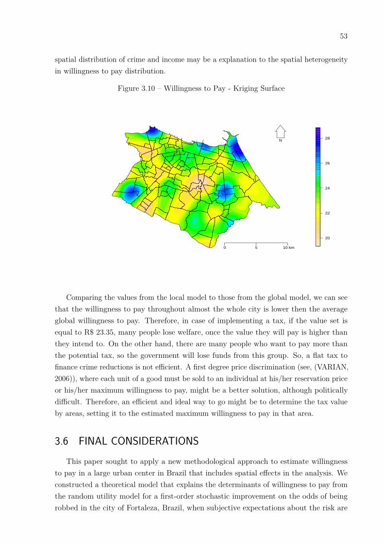
53

spatial distribution of crime and income may be a explanation to the spatial heterogeneityin willingness to pay distribution.

Figure 3.10 – Willingness to Pay - Kriging Surface

20

22

24

26

28

0 5 10 km

N

Comparing the values from the local model to those from the global model, we can seethat the willingness to pay throughout almost the whole city is lower then the averageglobal willingness to pay. Therefore, in case of implementing a tax, if the value set isequal to R$ 23.35, many people lose welfare, once the value they will pay is higher thanthey intend to. On the other hand, there are many people who want to pay more thanthe potential tax, so the government will lose funds from this group. So, a flat tax tofinance crime reductions is not efficient. A first degree price discrimination (see, (VARIAN,2006)), where each unit of a good must be sold to an individual at his/her reservation priceor his/her maximum willingness to pay, might be a better solution, although politicallydifficult. Therefore, an efficient and ideal way to go might be to determine the tax valueby areas, setting it to the estimated maximum willingness to pay in that area.

3.6 FINAL CONSIDERATIONSThis paper sought to apply a new methodological approach to estimate willingness

to pay in a large urban center in Brazil that includes spatial effects in the analysis. Weconstructed a theoretical model that explains the determinants of willingness to pay fromthe random utility model for a first-order stochastic improvement on the odds of beingrobbed in the city of Fortaleza, Brazil, when subjective expectations about the risk are

54

available. We showed that the determinant factors explaining willingness to pay in the cityof Fortaleza are Subject Prob*Income, Gender, Age, Education, Perception of patrollingand Victim of robbery.

From the global model, we estimated a mean WTP of R$ 23.35 per month/household asthe value that the representative citizens of Fortaleza would be willing to pay to reduce theamount of robberies in the city in 50%. From this value, we calculated in approximatelyR$ 198.92 million the total cost to society, equal to 20.63% of the total amount spent onpublic security in the state of Ceará in 2011. We also estimated the WTP per robberyavoided equal to R$ 11,969.

Our local model, utilizing an adaptive gaussian kernel function with a bandwidth equalto approximately 0.6149, estimated a geographically weighted regression with an intervalregression that, to the best of our knowledge, it is the first study to do so. We showedthat in almost the whole city, the willingness to pay estimated in the local model is lowerthan one estimated in the global model and that there is an island where this value isgreater. So, in case of tax implementation, the most efficient procedure is to discriminatethe tax according to the area.

As suggestions for future studies, we believe that the construction of a new modelrelaxing the hypothesis of risk neutrality is a fine way to go. Finally, replicating ourempirical exercise on different data sets coming from different institutional backgroundsmight be something worth pursuing in order to validate our approach.

REFERENCES

ALMEIDA, E. Econometria espacial aplicada. [S.l.]: Alínea, 2012.

ARAÚJO, A. F. V. d.; RAMOS, F. S. Estimação da perda de bem-estar causada pelacriminalidade: o caso da cidade de João Pessoa - pb. Economia, v. 10, n. 3, p. 577–607,set/dez 2009.

ATKINSON, G.; HEALEY, A.; MOURATO, S. Valuing the costs of violent crime: astated preference approach. Oxford Economic Papers, v. 57, n. 4, p. 559–585, 2005.

BIVAND, R.; PEBESMA, E.; GÓMEZ-RUBIO, V. Applied spatial data analysis with R:analysis with R. [S.l.]: Springer, 2008. (Use R!). ISBN 9780387781716.

BIVAND, R.; YU, D. spgwr: geographically weighted regression. [S.l.], 2013. R packageversion 0.6-24. Disponível em: <http://CRAN.R-project.org/package=spgwr>.

BOWEN, H. R. The interpretation of voting in the allocation of economic resources.Quarterly Journal of Economics, v. 58, p. 27–48, 1943.

CAMERON, T. A.; DESHAZO, J. Demand for health risk reductions. Journal ofEnvironmental Economics and Management, v. 65, n. 1, p. 87–109, 2013.

CAMERON, T. A.; DESHAZO, J.; STIFFLER, P. Demand for health risk reductions: across-national comparison between the us and canada. Journal of Risk and Uncertainty,v. 41, n. 3, p. 245–273, 2010.

CAMERON, T. A.; HUPPERT, D. D. Ols versus ml estimation of non-market resourcevalues with payment card interval data. Journal of Environmental Economics andManagement, v. 17, n. 3, p. 230 – 246, 1989.

CARSON, R. T.; HANEMANN, W. M. Handbook of environmental economics:valuing environmental changes. In: . [S.l.]: Elsevier Science, 2005. (Handbookof Environmental Economics, v. 2), cap. 17.Contingent Valuation, p. 822–920. ISBN9780080457499.

CARVALHO, J. R. Montagem de uma base de dados longitudinal de vitimização do ceará:aspectos sócio-econômicos and espaciais. Relatório Final, FUNCAP. 2012.

CIRIACY-WANTRUP, S. V. Capital returns from soil-conservation practices. Journal ofFarm Economics, v. 29, p. 1181–1196, 1947.

COHEN, M. A. et al. Willingness-to-pay for crime control programs. Criminology, v. 42,n. 1, p. 89–110, 2004.

56

DRUCK, S. et al. Análise espacial de dados geográficos. EMBRAPA, 2004. Disponível em:<www.dpi.inpe.br/gilberto/livro/analise>.

ESTATÍSTICA, I. B. de Geografia e. Censo demográfico 2010. 2012.Http://www.censo2010.ibge.gov.br/apps/mapa/. Acessado em: 25/10/2012.

FOTHERINGHAM, A. S.; BRUNSDON, C.; CHARLTON, M. Geographically weightedregression: the analysis of spatially varying relationships. [S.l.]: John Wiley & Sons, 2003.

HENNINGSEN, A.; TOOMET, O. maxlik: A package for maximum likelihoodestimation in R. Computational Statistics, v. 26, n. 3, p. 443–458, 2011. Disponível em:<http://dx.doi.org/10.1007/s00180-010-0217-1>.

HOYOS, D.; MARIEL, P. Contingent valuation: past, present and future. PragueEconomic Papers, v. 2010, n. 4, p. 329–343, 2010.

JORGENSEN, B. et al. Protest responses in contingent valuation. Environmental andResource Economics, v. 14, n. 1, p. 131–150, July 1999.

LUDWIG, J.; COOK, P. J. The benefits of reducing gun violence: evidence fromcontingent-valuation survey data. Journal of Risk and Uncertainty, v. 22, n. 3, p. 207–26,2001.

MAS-COLELL, A.; WHINSTON, M. D.; GREEN, J. R. Microeconomic theory. [S.l.]:Oxford University Press, 1995.

PúBLICA, F. B. de S. Anuário brasileiro de segurança pública. [S.l.], 2012.

R Core Team. R: a language and environment for statistical computing. Vienna, Austria,2014. Disponível em: <http://www.R-project.org/>.

SOEIRO, M.; TEIXEIRA, A. A. Determinants of higher education students’ willingness topay for violent crime reduction: a contingent valuation study. [S.l.], July 2010. Disponívelem: <http://ideas.repec.org/p/por/fepwps/384.html>.

STRAZZERA, E. et al. The effect of protest votes on the estimates of wtp for use valuesof recreational sites. Environmental and Resource Economics, v. 25, n. 4, p. 461–476,August 2003.

VARIAN, H. Microeconomia - Principios básicos. [S.l.]: CAMPUS, 2006. ISBN9788535216707.

WHITEHEAD, J. C.; BLOMQUIST, G. C. Handbook on contingent valuation. In: .[S.l.]: Edward Elgar Publishing Limited, 2006. cap. The Use of Contingent Valuation inBenefit Cost Analysis, p. 92–115.

4 PEER EFFECTS AND ACADEMIC PER-FORMANCE IN HIGHER EDUCATION -A REGRESSION DISCONTINUITY DE-SIGN APPROACH

4.1 INTRODUCTIONHuman beings are social creatures. This is based not only on the fact that we like

company or depend on each other. Human beings are social creatures simply in the sensethat our existence requires interaction with other people (GAWANDE, n.d). In the lastdecades, economists have devoted great attention to these interactions and its influenceon individual behavior. The effects of these interactions are known in the literature as“peer effects”.

Sacerdote (2011) defines peer effect as any externality, excluding those market-based orprice-based, in which peers’ background, current behavior, or outcomes exert an influenceon a specific outcome obtained by another individual. Manski (1993) classifies this effectas endogenous, when it emanates from peers’ current outcomes, and exogenous, when it isdue to peers’ backgrounds.

Several studies have analyzed peers’ influence on criminal activity, drugs use, teenagepregnancy, educational achievement, among others (SACERDOTE, 2011). Lookingspecifically at the literature concerning educational achievement, peer effects have playedan important role for primary and secondary education since Coleman et al. (1966)seminal work, being considered a key factor in determining children’s schooling outcomes(WINSTON; ZIMMERMAN, 2004).

Even though the importance of peer effects in elementary and secondary educationhad been raised a long time ago, its relevance to the economics of undergraduate/graduatedegrees has only recently been acknowledged (WINSTON; ZIMMERMAN, 2004). Thence-forward, this research agenda experimented an exponential growth, with several studiesseeking to take a deeper look at the peer effects for higher education. So far, the empiricalresults bring up contradictory conclusions. Some studies find a positive effect on academicoutcomes due to peers’ influence, while others show negative effects or even no effect at all(EPPLE; ROMANO, 2011; SACERDOTE, 2011).

Commonly, the literature has been using roommates interaction as a standard sourceof peer effects. This is the case for works such as Sacerdote (2001),Zimmerman (2003) andMcEwan and Soderberg (2006). On the other hand, studies like Paola and Scoppa (2010),

58

Androushchak, Poldin and Yudkevich (2012) and Booij, Leuven and Oosterbeek (2015)prefer to take advantage of classmates interactions. Our paper follows this guidance anduses the interactions between classmates as well. However, it contributes to the literaturepresenting a different group formation.

Based on this set of papers, we believe our endeavor has its own merits. Firstly, weestimate peer effects in higher education for a developing country with an institutionalbackground which is very different from what is found in OECD members, for example.Secondly, by aggregating new methodological procedures, we can better understand therelation between peer effects and academic performance in high education.

Therefore, this paper aims to estimate peer effects of undergraduate students onacademic outcomes. For this purpose, we used a micro data set conceded by the FederalUniversity of Ceará, a public Brazilian university located in Fortaleza, the capital cityof Ceará. Our data set brings several socioeconomic information and maps concerning 4years of academic performance with respect to 2149 students enrolled in 33 undergraduateprograms. Due to the entrance process specificities, we are able to estimate peer effectsusing a sharp regression discontinuity design. Also, in light of programs’ heterogeneity,and since the assignment grade distribution pattern is different, we are able to estimatea multi-treatment effect model. For this, we classify each program according to thecompetition in its first and second semester classes.

We found that peer effects have a negative impact on the academic performance ofour undergraduate students. The evidence suggests that low-ranked students put togetherwith high-ranked classmates have a worse academic performance than those in a lowerlevel class. This goes against several studies of peer effects for primary and high schools,as well as for higher education.

Notwithstanding, for a multi treatment model, we also found evidence of non-linearitiesas in Sacerdote (2001) and Zimmerman (2003). We found positive peer effects whenboth first and second semester classes are of low competition level, and negative peereffects in all other configurations, with modest magnitudes when both classes are of highcompetition level.

Besides this introduction and a final considerations section, this paper presents fivemore sections. Section 2 offers a brief literature review of peer effects on academic outcomes.Section 3 introduces the entrance process for Brazilian universities and demonstrates thatit follows a sharp design. Section 4 scrutinizes our data, presenting the results of an initialexploratory analysis. Section 5 sets up the model to be estimated and a brief discussion ofthe estimation method. Finally, section 6 presents our results.

59

4.2 BRIEF EMPIRICAL LITERATURE REVIEW

4.2.1 Peer effects

The literature of peer effect on academic achievement has grown significantly in recentyears. Studies trying to access its role in elementary, secondary and post-secondary educa-tional levels are of particular interest in many countries, raising different methodologicalapproaches to take the particularities of each educational level and backgrounds intoaccount.

Sacerdote (2001) estimated peer effects among Dartmouth College (USA) roommates.He found that peers have an important impact on students’ grades and on the decision tojoin social groups such as fraternities. Also, the paper attests a non-linearity in these peereffects: students whose roommates were in the top 25% of the class had higher grades.Sacerdote (2001) concluded that high-ability students had a positive effect on the academicachievement of relatively less talented colleagues, while there was no such influence forstudents in the middle of distribution.

Similarly, Zimmerman (2003) studied peer effects among Williams College (USA)undergraduate students. In this paper, since first year roommates were assigned randomlywith respect to academic ability, the author could estimate differences in grades of high,medium, and low SAT students living with high, medium or low SAT roommates. Theresults indicated that a medium student tended to have worse grades if put together witha low SAT roommate, while high ability students were least influenced by peers.

McEwan and Soderberg (2006), in a study carried out at Wellesley College (USA),estimated the effects of students’ background characteristics on their roommates’ academicoutcomes. The authors applied both a linear and a nonlinear model. Regarding the firststructure, there is no evidence of peer effects on students’ GPA. With respect to thenonlinear specification, the results suggest that students’ SAT scores have a nonlineareffect on their roommates’ achievement, yet the results are not robust. The conclusionis that there might exist roommate peer effects restricted to a small number of students.However this effect is not a key determinant for academic outcomes.

Carrell, Fullerton and West (2008) also estimated peer effects in college achievement.The paper uses data from the United States Air Force Academy, in a context in whichstudents are exogenously assigned to peer groups. The interaction is even stronger in thiscase, since required activities involve both academic and non-academic duties. They find ascholarly peer influence larger than those found in previous studies relating to roommates.Furthermore, peer effect persists at a diminishing rate into sophomore, junior, and senioryears, indicating long lasting ties on academic achievement.

Contreras, Badua and Adrian (2012) investigated peer effects for classroom colleaguesin a Business College of a U.S. public university. The authors find a negative significantpeer effect in students’ performance, yet the proper direction and magnitude are sensitive

60

to both peers’ and student’s own average ability.Besides the USA, there is a growing literature in European countries on peer effects. In

Italy, Paola and Scoppa (2010) analyzed peer effects among students of Calabria University,a middle-sized public university. They found a positive and statistically significant influence,being robust to different peer group definitions and abilities measures. Also, the effectwas larger than previous studies focusing on roommates. The results attest that students’ability is an important input in college education, which means that attracting high-levelstudents is a key path to improve the overall performance by means of direct and indirectdirections.

Androushchak, Poldin and Yudkevich (2012) used data about Russian undergraduatestudents enrolled at the Economics department of the National Research University —Higher School of Economics (HSE)— to estimate peer effects in exogenously formed groups.The evidence suggests that high-ability classmates exert a positive influence on individualacademic performances. Still, the most talented ones are the greatest beneficiaries fromthis presence. The paper also finds that an increase in the proportion of low-performancestudents has an insignificant or negative influence on individual grades.

Regarding undergraduate students in Economics at the University of Amsterdam(NED), Booij, Leuven and Oosterbeek (2015) estimated peer effects from tutorial groups’ability composition. Aiming to achieve a wide range of support, the authors manipulatedthese compositions and assigned the students randomly. They find that low and mediumability students gain, on average, 0.2 standard deviation achievement units after switchingfrom ability mixing to three-way tracking — a system in which each group is constitutedby students of the same ability distribution, measured by GPA. They also find that high-ability students are not affected by the specific group composition, and defend that there isno evidence implying that teachers adjust their teaching to different group configurations.

4.2.2 The use of regression discontinuity design

In common, none of these papers use a regression discontinuity design approach toestimate peer effects in academic achievement. Actually, this approach is usually foundin analysis of both remedial education effects and financial aid on academic achievement,due to particularities of post-secondary educational level.

Moss and Yeaton (2006) are an example of a sharp regression discontinuity designapplication in remedial education. This study analyzed the effectiveness of a developmentalEnglish program in an American university. The program offers compulsory remedialeducation to students of ASSET scores less or equal to 85 out of 107 points. Theauthors found that those students participating in the program had their English academicachievement similar to those initially out of supplemental coursework. Furthermore, thestudents in greatest need of the program had the major benefit from it.

61

Another example is the study of Butcher, McEwan and Taylor (2010). It estimated thecausal effect of taking a course in quantitative reasoning on student’s academic performanceand classroom peer-group composition at Wellesley College (USA). The assignment rule inthis program is similar to the one presented in Moss and Yeaton (2006): if the student’stest score is less or equal to 9 (out of 18), then he/she is assigned to this mandatoryquantitative course. The authors found that there is no impact in taking the course onstudent’s academic outcomes. Nevertheless, they identified robust effects on classroompeer-group composition, i.e, classmates of this remedial course tend to keep studyingtogether along other different courses.

In a similar study, Schöer and Shepherd (2013) estimated the role of taking a compulsoryremedial course on students’ performance in an undergraduate level microeconomics class.Using data from a South African university, they used a fuzzy regression discontinuitydesign and found that this program participation positively affects students’ performance.

Regarding the role of financial aid on academic outcomes, the seminal paper of Klaauw(2002) analyzed the effects of universities’ financial aid offers on students enrollmentdecisions. The author found that this recruitment resource is an effective instrument incompeting with other colleges for new students. In the same line, Leeds and DesJardins(2014) found similar conclusions for the University of Iowa. In addition, the results suggestthat financial aids may have strong effects on the brightest candidates.

Mealli and Rampichini (2012) analyze the relation between grants offered by an Italianuniversity for low-income students and their dropout decision. The results suggest that,at a given threshold, the grant is an effective tool to prevent those low-income studentsto drop out of higher education. However, if the family income is much lower than thisthreshold, then the grant effect becomes smaller and not significant.

Canton and Blom (2004) analyzed the effects of financial aid on enrollment and students’performance at Mexican universities. The results indicate a positive effect for both issues.Concerning the enrollments, a strong impact is verified, since the probability of enteringin higher education is raised in 24 percent. For the performances, students who receivefinancial aid have better academic results than those without it. A similar study wascarried out by Curs and Harper (2012), attesting that students who receive financial aidhave a GPA between 0.12 and 0.16 higher than students who do not.

In the studies of peer effects, the methodological framework depicted by the regressiondiscontinuity design is more usual when dealing with elementary and high school levels.For example, Koppensteiner (2012), using Brazilian data on elementary school students,estimated the effect of being in a class of older classmates on students’ achievement. Theconclusion consists in a large negative impact of it. Card and Giuliano (2015) estimatedthe effect of being in a gifted/high achiever classroom for U.S. students. They foundpositive and significant effects concentrated among minorities, and found no evidence ofspillovers on non-participants of the program.

62

The same Card and Giuliano (2015) motivation is presented in Vardardottir (2013).Refering to high school Icelander students, this paper estimated the effect of being inhigh-ability classes, and found a significant and sizable positive impact on the academicachievement of students around the assignment threshold. Abdulkadiroğlu, Angrist andPathak (2014) are also concerned about peer effects at a high school level. They estimatedthe effect of study in a high-quality school, and the results suggest that the marked changesin peer characteristics at exam school admissions cutoffs have little causal effect on testscores or college quality.

In common, all of these studies follow a clear rule in the class group formations, whichare usually not the case for U.S. and European universities. With respect to Brazil, thereis a well-established rule in forming two types of undergraduate classes: the first one getsthe best ranked students in the entrance process, and start academic activities in February(first semester); the second type is a place for the lowest ranked students, and runs at thebeginning of August (second semester). Relying on this fact, we developed our study.

4.3 THE ENTRANCE PROCESS IN BRAZILIAN UNIVERSITIESIn Brazil, according to (Inep) (2014), in 2013, there were 7,3 million students enrolled

in 2,391 higher education institutions. Among those institutions, 106 are public andmaintained by the Brazilian federal government, counting 5.968 undergraduate programsand 1,14 million students enrolled at federal institutions. In other terms, these num-bers represent 18% and 15% of Brazilian undergraduate programs and college students,respectively.

Since federal universities are free of charge and present a high teaching quality1, theyare target of many students from all social backgrounds, which translates into a highdemand and, therefore, great competition for a vacancy. Thus, in order to ensure equalaccess, its entrance processes take place by means of a public tender.

Silva (2007) makes a historical analysis of the admission process in higher education inBrazil. In the 19th century, students who aimed to enter in higher education had to gothrough a series of tests after they completed the secondary education to obtain a requiredgrade to access the higher education. These exams were called exit tests.

From 1915 on, these exams became to be called Vestibular, as we know nowadays,being mandatory for all students who wanted to access the higher education system. Thisadmission process became effective, in fact, in the 1920s, when the number of candidatesbecame higher than the number of vacancies. In this period, Vestibular still was an exittest.

It was after 1925 that Vestibular became an entry test, whose objective was to evaluatestudent’s capability to understand studies at higher level. The exams were restricted to1 In Brazil, public universities hold status of higher quality compared to their private counterparts.

63

disciplines considered pre-requisites to the undergraduate program the student intendedto attend to.

In 1971, due to the pressure of the students who were unable to access higher education,new conditions of access were created. This new system established that Vestibular musthave only one content for all programs and adopt classification criteria, in which studentsthat obtained the greatest grades were selected. Under this system, each university becameresponsible to organize its own selection process, establishing the number of vacancies tobe offered (SILVA, 2007). This system remained in force until 2010, when a new admissionprocess based on ENEM and SISU arose2.

Abreu (2013) summarizes Vestibular’s algorithm. In a first moment, each studentchooses and announces only one program of his preference. In a second moment, for eachprogram, a preference relation is determined, utilizing the grade obtained in the exam.And finally, students are allocated based on their rankings and preferences of the chosenprogram. It was demonstrated that this algorithm is not stable, is not pareto efficient andis not strategy-proof.

At the time of our analysis, the Federal University which we have access to theinformation used Vestibular as its admission process. In this University, the exam consistsin two stages. The access to the second stage is conditioned by the performance in the firststage. All students above a rank at the first stage exam are accepted to the second stage,which make the number of students who take the second stage exam a multiple (usually 4sometimes 3) of the number of final available vacancies. These ranks (one for each major)define a first stage grade threshold. Similarly, second stage threshold determine who passesthe exam and enters the University (CARVALHO; MAGNAC; XIONG, 2014). Based onscores achieved in the second stage, students were ranked, vacancies were filled, and theupper classified half of students for every course was assigned to start studies in the firstsemester of the academic year (first semester class), while the bottom half was allocatedinto the second semester(second semester class).

Carvalho, Magnac and Xiong (2014) demonstrated that this threshold is a BayesianNash equilibrium, and it is unique. This allows us to use a sharp regression discontinuitydesign to analyze peer effects among students allocated in first semester classes and insecond semester classes.

4.4 DATAOur analysis is based on a rich administrative data set, providing information on

undergraduate students enrolled in 2008 at the Federal University of Ceará (UFC). This is2 Since 2011, the new entrance process is by means of ENEM and SISU. Students take a centralized

national exam (ENEM) and, in light of the obtained results, they choose any university and under-graduate program (SISU), taking their own score and the cutoff score determined by competition intoaccount.

64

a public Brazilian university located in Fortaleza — the fifth largest city in Brazil with apopulation of 2.5 million citizens. Founded in 1954, UFC is considered one of the bestuniversities in Brazil according to the Brazilian ministry of education, and the secondbest in the northeastern region. During the 2013 academic year, the university had 26,782students enrolled in 114 undergraduate programs. With respect to graduate programs, theuniversity had 6,061 students enrolled in 167 programs, divided into lato sensu, professionaland academic masters, as well as doctoral programs. The Federal University of Cearáwas constituted by 2,152 professors, of whom 1,436 and 543 have doctoral and master’sdegrees, respectively. UFC also had 3,407 administrative staff members, including theUniversity Hospital (UFC, 2014).

The data set was collected from both the Vestibular Commission and the provostOffice of Undergraduate Studies. We have information on 27 undergraduate programswith classes starting in both academic terms3, counting 1550 students. Our data coversgrades and final classification in the entrance exam for the 2008 academic year. Wealso bring information on the students’ socioeconomic characteristics, collected at theregistration stage by means of a survey held by the Vestibular commission. Concerningacademic performance, students are traced from 2008 to 20114, which is equivalent to 8academic semesters and to the required time before graduating. As a measure of academicachievement, we use IRA — UFC equivalent to the American GPA.

The IRA (Índice de Rendimento Acadêmico) index is a measure of student’s academicperformance similar to the American GPA, but in a 10-point scale. This index is used torank students for research and teaching grants, for distinction purposes and so on. TheIRA index for a student i is calculated as follows:

IRAi =(

1− 0.5TC

)×(∑

j Pi × Cj ×Nj∑j Pj × Cj

)(4.1)

Where:

•T is the sum of all withdrawn courses’ workload;

•C is the sum of all courses’ workload, withdrawn or not;

•Cj is the workload of course j;

•Nj is the final grade of course j;

•Pj is the period in which the course was done, obeying the following limitation: Pj= min {6, semester in which the course was done}.

As shown above, the IRA index is a weighted mean. Variable TCmeasures the proportion

of all withdrawn courses’ workload with respect to the total amount (withdrawn or not).3 This is equivalent to 38% of the total amount of undergraduate programs.4 Or until student drops out the course.

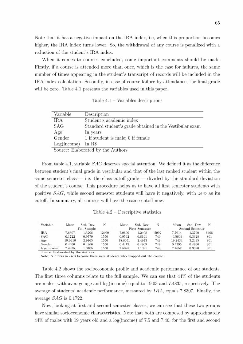
65

Note that it has a negative impact on the IRA index, i.e, when this proportion becomeshigher, the IRA index turns lower. So, the withdrawal of any course is penalized with areduction of the student’s IRA index.

When it comes to courses concluded, some important comments should be made.Firstly, if a course is attended more than once, which is the case for failures, the samenumber of times appearing in the student’s transcript of records will be included in theIRA index calculation. Secondly, in case of course failure by attendance, the final gradewill be zero. Table 4.1 presents the variables used in this paper.

Table 4.1 – Variables descriptions

Variable DescriptionIRA Student’s academic indexSAG Standard student’s grade obtained in the Vestibular examAge In yearsGender 1 if student is male; 0 if femaleLog(income) In R$Source: Elaborated by the Authors

From table 4.1, variable SAG deserves special attention. We defined it as the differencebetween student’s final grade in vestibular and that of the last ranked student within thesame semester class — i.e. the class cutoff grade — divided by the standard deviationof the student’s course. This procedure helps us to have all first semester students withpositive SAG, while second semester students will have it negatively, with zero as itscutoff. In summary, all courses will have the same cutoff now.

Table 4.2 – Descriptive statistics

Variable Mean Std. Dev. N Mean Std. Dev. N Mean Std. Dev NFull Sample First Semester Second Semester

IRA 7.8307 1.3208 12400 7.9690 1.2408 5992 7.7014 1.3790 6408SAG 0.1722 0.9779 1550 0.9562 0.8191 749 -0.5609 0.3328 801Age 19.0316 2.9165 1550 18.8051 2.4943 749 19.2434 3.2495 801Gender 0.4406 0.4966 1550 0.4419 0.4969 749 0.4395 0.4966 801Log(income) 7.4835 1.0105 1550 7.5025 1.1091 749 7.4657 0.9090 801Source: Elaborated by the AuthorsNote: N differs in IRA because there were students who dropped out the course.

Table 4.2 shows the socioeconomic profile and academic performance of our students.The first three columns relate to the full sample. We can see that 44% of the studentsare males, with average age and log(income) equal to 19.03 and 7.4835, respectively. Theaverage of students’ academic performance, measured by IRA, equals 7.8307. Finally, theaverage SAG is 0.1722.

Now, looking at first and second semester classes, we can see that these two groupshave similar socioeconomic characteristics. Note that both are composed by approximately44% of males with 19 years old and a log(income) of 7.5 and 7.46, for the first and second

66

group, respectively, in average. The academic performance of the first semester group is7.96, and 7.70 to the second.

Finally, by definition, variable SAG has a positive or negative sign depending on thereference class — first or second semester, respectively. Concerning the spread of SAG,the standard deviation in the first group is larger than in the second, which shows thatthe class beginning in the last academic semester is more homogeneous. This is not acoincidence, since students ranked in the top class tend to be more prepared and achievehigher grades in vestibular. It also involves the top 1% students, whose grades are possiblytoo far from average. We can see this better in figures 4.1, 4.2, 4.3, 4.4 and 4.5.

67

Figure 4.1 – Distribution of normalized assignment grade by courses - Medical school andLaw school

|

|

|

|||

||||||

Dire

ito (

Diu

rno)

Dire

ito (

Not

urno

)

Enf

erm

agem

Farm

acia

Med

icin

a (F

orta

leza

)

Odo

ntol

ogia

(Fo

rtal

eza)

−4.0

−3.5

−3.0

−2.5

−2.0

−1.5

−1.0

−0.5

0.0

0.5

1.0

1.5

2.0

2.5

3.0

3.5

Nor

mal

ized

ass

ignm

ent g

rade

Undergraduate courses

These figures display the SAG distribution for each course. Figures 4.1, 4.2, 4.3 and

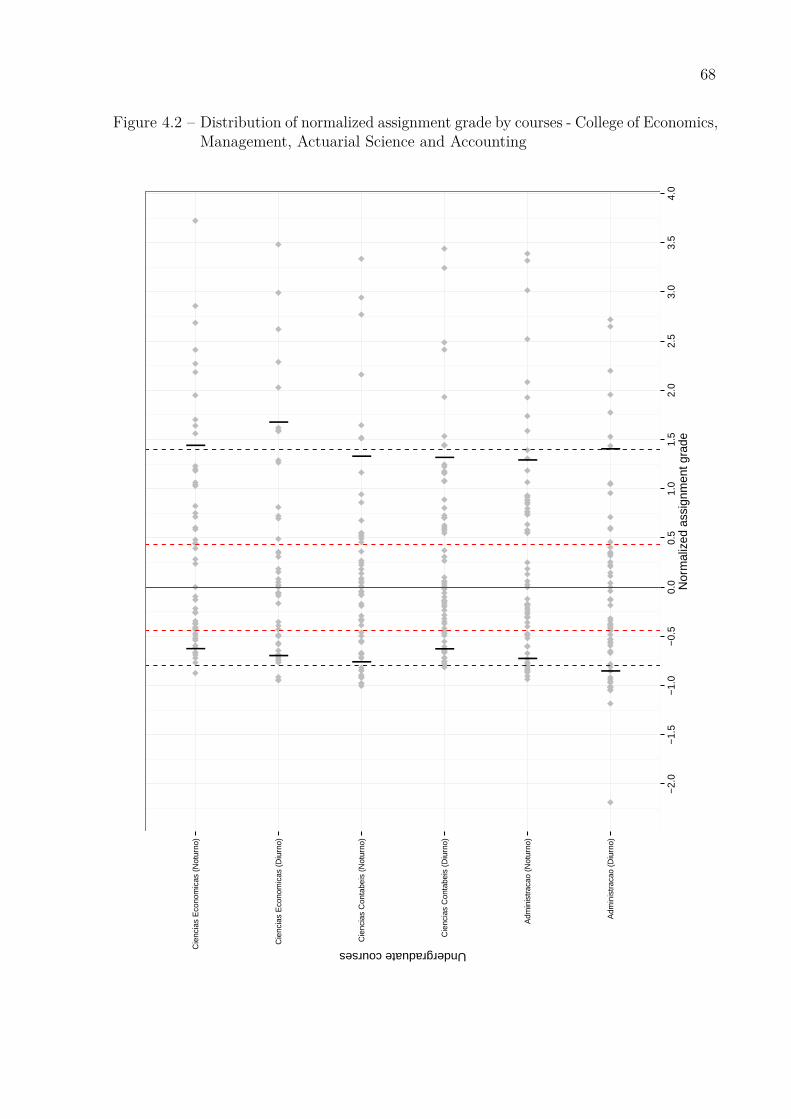
68

Figure 4.2 – Distribution of normalized assignment grade by courses - College of Economics,Management, Actuarial Science and Accounting

||||

|

|

|

||

|||

Adm

inis

trac

ao (

Diu

rno)

Adm

inis

trac

ao (

Not

urno

)

Cie

ncia

s C

onta

beis

(D

iurn

o)

Cie

ncia

s C

onta

beis

(N

otur

no)

Cie

ncia

s E

cono

mic

as (

Diu

rno)

Cie

ncia

s E

cono

mic

as (

Not

urno

)

−2.0

−1.5

−1.0

−0.5

0.0

0.5

1.0

1.5

2.0

2.5

3.0

3.5

4.0

Nor

mal

ized

ass

ignm

ent g

rade


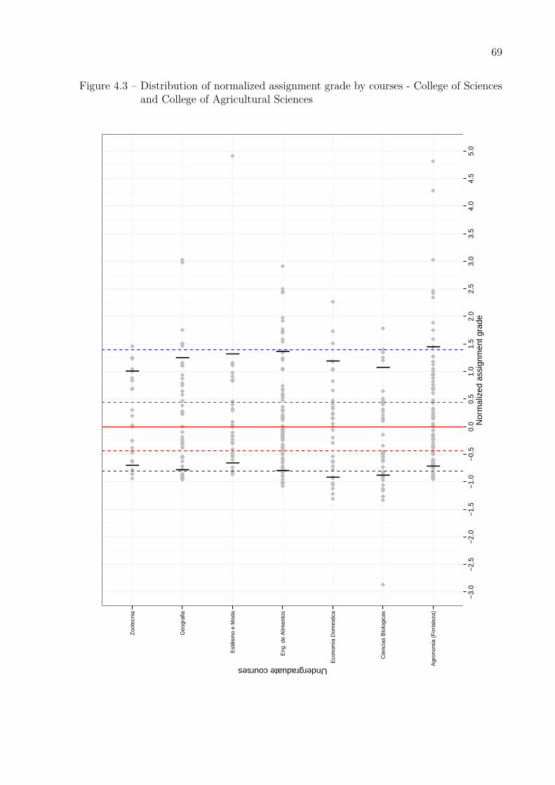
69

Figure 4.3 – Distribution of normalized assignment grade by courses - College of Sciencesand College of Agricultural Sciences

|

||

|||

|

|

||||||

Agr

onom

ia (

Fort

alez

a)

Cie

ncia

s B

iolo

gica

s

Eco

nom

ia D

omes

tica

Eng

. de

Alim

ento

s

Est

ilism

o e

Mod

a

Geo

graf

ia

Zoo

tecn

ia

−3.0

−2.5

−2.0

−1.5

−1.0

−0.5

0.0

0.5

1.0

1.5

2.0

2.5

3.0

3.5

4.0

4.5

5.0

Nor

mal

ized

ass

ignm

ent g

rade


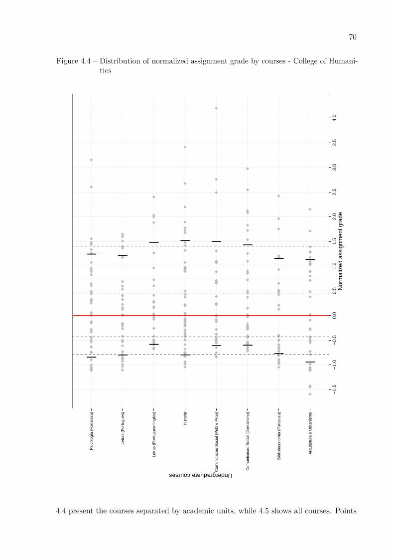
70

Figure 4.4 – Distribution of normalized assignment grade by courses - College of Humani-ties

||

||||

||

|

|

||

|

|

||

Arq

uite

tura

e U

rban

ism

o

Bib

liote

cono

mia

(Fo

rtal

eza)

Com

unic

acao

Soc

ial (

Jorn

alis

mo)

Com

unic

acao

Soc

ial (

Pub

l e P

rop)

His

toria

Letr

as (

Por

tugu

es−I

ngle

s)

Letr

as (

Por

tugu

es)

Psi

colo

gia

(For

tale

za)

−1.5

−1.0

−0.5

0.0

0.5

1.0

1.5

2.0

2.5

3.0

3.5

4.0

Nor

mal

ized

ass

ignm

ent g

rade


4.4 present the courses separated by academic units, while 4.5 shows all courses. Points

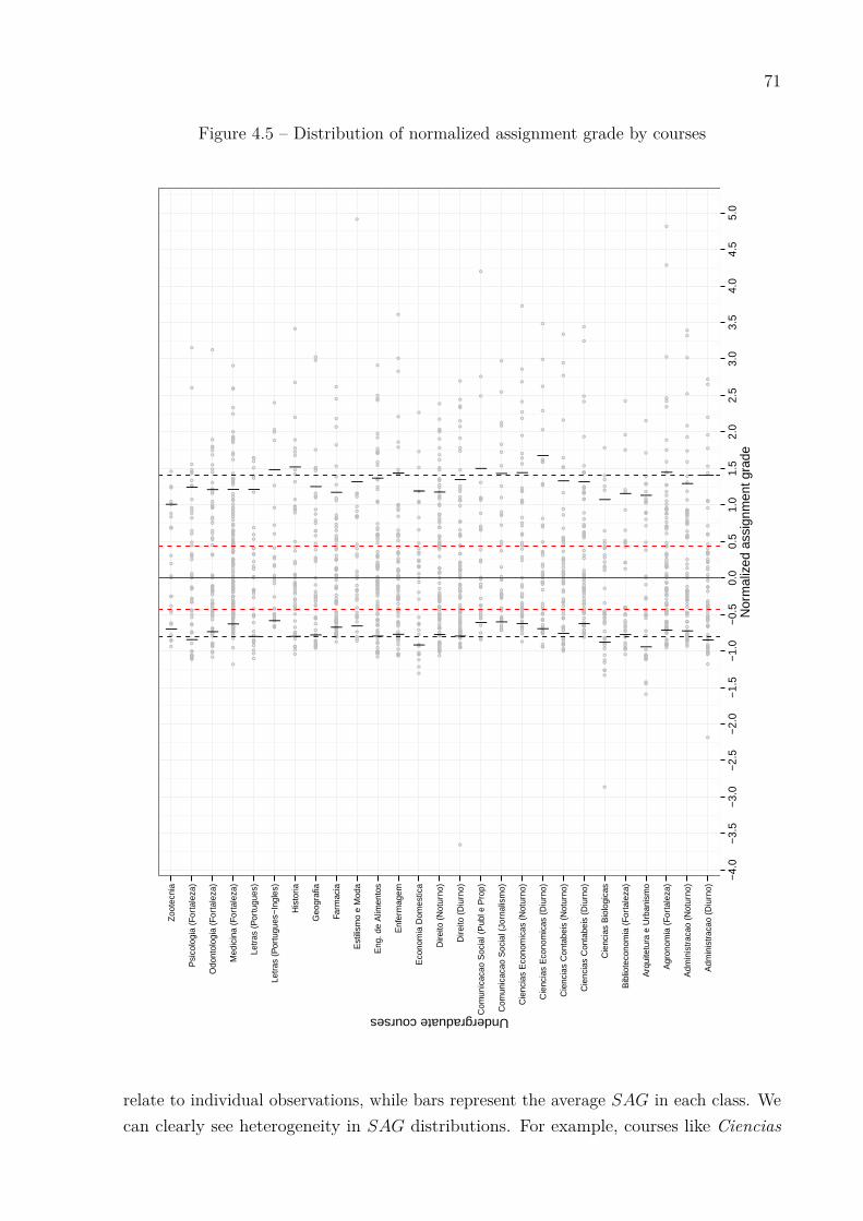
71

Figure 4.5 – Distribution of normalized assignment grade by courses

●

●

●

●

●

●

●

●

●

●

●

●● ●●

●

●

●

●

●●

●

●

●

●

●

●

●

●

●

●

●●

●

●

●

●

●

●

●

●

●

●

●

● ●

●

●

●

●

●

●

●●

●

●

●

●

●●

●

●

●

●

●

●

●

●

●

●

●

●

●

●

●

●

●

●

●

●

●

●

●●

●●

●

●

●●

●

●

●

●

●

●

●●

●

●

●

●

●

●

●

●

●

●

●

●

●

●

●

●●

●

●

●

●

●

●

●

●

●

●

●

●

●

●

●

●

●

●

●

●

●●

●

●

●

●

●

● ●

●

●

●

●

●

●

●

●

●

●

●

●

●

●

●

●

●

●

●

●

●

●

●

●

●

●

●

●●

●

●

●

●

●

●

●

● ●

●

●

●

●

●

●

●

●

●

●

●●

●

●

●

●

●●

●

●

●

●

●

●

●

●

●

●

●

●

●

●

●

●

●

●

●

●

●

●

●

●

●

●

●

●

●

●

●

●

●

●

●

●

●

●

●

●

●

●

●

●●

●

●

●

●

●

●

●

●

●

●

●

●

●

●

●

●

●

●

●

●

●

●

●

●

●

●

●

●

●

●

●

●

● ●

●

●

●

●

●

●

●

●

●

●

●

●

●

●

●

●●

●

●

●

●

●

●

●

●

●

●

●

●

●

●

●

●

●

●

●

●

●

●

●

●

●

●

●

●

●●

●●

●

●

●

●

●

●

●

●

●

●

●●

●

●

●

●

●

●

●

●

●

●

●

●●

●

●

●

●

●●

●

●

●

●

●●

●

●

●

●

●

●

●

●

●

●

●

●

●

●

●

●

●

●

●

●

●

●

●

●

●

●

●

●

●

●

●

●

●

●

●

●

●

●

●

●

●

●

●

●

●

●

●

●

●

●●

●

●

●●

●

●

●

●

●

●

●

●

●

●

●

●

●

●

●

●

●

●

●

●

●

●

●

●

●

●

●

●

●

●●

●

●

●

●●

●

●

●

●

●

●

●

●

●

●

●

●

●

●

●

●

●

●

●

●

●

●

●●

●

●

●

●

●

●●

●

●

●

●

●

●

●

●

●

●

●●●

●

●

●

●

●

●

●

●

●

●

●

●

●

●

●

●

●

●

●

●

●

●

●

●

●

●

●

●

●

●

●

●

●

●

●

●

●

●

●

●

●

●●●

●

●

●

●

●

●

●

●

●

●

●

●

●

●

●

●

●

●

●

●

●

●

●●

●

●

●

●

●

●

●

●

●

●

●

●

●

●

●

●

●

●

●

●

●

●

●

●

●

●

●

●●

●●

●

●

●

●

●

●

●

●

●

●

●

●

●

●

●

●

●●

●

●

●

●

●

●●

●

●

●●

●

●

●

●

●

●

●

●● ●

●

●

●

●

●

●

●

●

●

●

●

●

●

●

●

●

●

●

●

●

●

●

●

●

●

●

●

●

●

●

●

●

●

●

●

●

●

●

●

●

●

●

●

●

●

●

●

●

●

●

●

● ●

●

●

●

●

●

●

●

●

●

●

●

●

●

●

●

●

●

●

●

●

●

●

●

●

●

●

●

●

●

●

●

●

●

●

●

●

●●

●

●

●

●

●

●

●

●

●

●

●

●

●

●

●

●

●

●

●

●

●

●

●●

●

●

●

●

●

●

●

●

●

●

●

●

●

●

●

●

●

●●

●

●

●

●

●

●

●

●

●

●

●

●

●

● ●●

●

●

●

●

●

●

●

●

●

●

●●

●

●

●

●

●

●

●

●

●

●

●

●

●

●

●

●

●

●

●

●

●

●

●

●

●

●

●

●

●

●●

●

●

●

●

●

●

●

●

●

●

●

●

●

●

●

●

●

●

●

●

●

●

●

●

●

●

●

●

●

●●

●●

●

●●

●

●

●

●

●

●

●

●●

●

●

●

●

●

●

●

●

●

●

●

●

●

●

●

●

●

● ●

●

●

●

●

●

●

●

●

● ●

●

●

●

●

●

●

●

●

●

●

●

●●

●

●

●

●●

●

●

●

●

●

●●

●

●

●

●

●

●

●

●

●

●

●

●

●

●

●●

●

●

●

●

●

●

●

●

●

●

●

●

●

●

●

●

●

●

●

●

●

●

●

●

●

●

●

●

●

●

●

●

●

●

●

●

●

●

●

●

●

●

●●

●

●

●

●●

●

●

●

●

●

●

●

●●

●

●

●

●

●

●

●

●●

●

●

●

●

●

●

●

●

●●

● ●

●

●

●

●

●●

●

●

●

●

●

●●

●

●

●

●

●

●

●

●

●

●

●

●

●

●●

●

●

●

●

●

●

●

●

●

●

●

●

●

●

●

●

●

●

●

●

●

●

●

●

●

●

●

●

●

●

●●

●●

●

●

●

●

●

●

●

●●

●

●

●●

●

●

●

●

●

●

●

●

●

●

●

●

●

●

●

●

●

●

●

●

●

●

●

●

●

●

●

●

●

●

●

●

●

●

●

●

●

●

●

●

●

●

●

●

●

● ●

●

●

●●

●

●

●

●

●

●

●

●

●

●●

●

●

●

●

●

●●

●

●

●

●

●●

●

●

●

●

●

●

●

●

●

●

●

●

●

●

●

●

●

●

●

●

●

●

●

●

●●

●

●

●

●

●

●

●

●

●

●

●

●

●●

●

●

●

●

●

●

●

●

●

●

●

●

●

●

●

●

●

●

●●

●

●

●●

●

●

●

●

●

●

●

●

●

●

●

●

●

●

●

●

●

●

●

●

●

●

●

●

●

●

●

●

●

●

●

●

●

●

●

●●

●

●

●

●

●

●

●

●

●

●

●

●

●

●

●

●

●●

●

●●

●

●

●

●

●

●

●

●

●

●

●

●

●

●

●

●

●

●

●

●

●

●

●

●

●

●

●

●

●

●

●

●

●

●

●

●

●

●

●

●

●

●

●

●

●

●●

●

●

●

●

●

●

●

●

●

●

●

●

●

●

●

●

●

●

●

●●

●

●

●

●

●

●

●

●

●

●

●

●

●

●

●

●

●

●

●

●

●●

●

●

●

●

●

●

●

●

●

●

●

●

●●

●

●

●

●

●

●

●

●

●

●

●

●

●

●

●

●

●

●●

●

●

●

●

●

●

●

●

●

●

●

●

●

●

●

●

●

●

●

●

●

●

●

●

●

●

●

●

●

●

●

●

●

●●

●

●

●

●

●

●

●

●

●

●

●

●

●

●

●

●

●

●

●

●

●

● ●

●

●

●

●

●

●

●

●

●

●

●

●

●

●

●

●

●

●

●

●

●

●

●●●

●

●

●

●

●

●●

●●

●

●

●

●

●

●

●

●

●

●

●

●

●

●

●

●

●

●

●

●

●

●

●

●

●

●

●

●

●

●●

●

● ●

●

●

●

●

||||

|

||

|||

|

||

||

||||

|

|

|||

||

|

|

|||

||

|

||

|| |||

|

|

|

|

|

| |

|

|

|

|

||

Adm

inis

trac

ao (

Diu

rno)

Adm

inis

trac

ao (

Not

urno

)

Agr

onom

ia (

Fort

alez

a)

Arq

uite

tura

e U

rban

ism

o

Bib

liote

cono

mia

(Fo

rtal

eza)

Cie

ncia

s B

iolo

gica

s

Cie

ncia

s C

onta

beis

(D

iurn

o)

Cie

ncia

s C

onta

beis

(N

otur

no)

Cie

ncia

s E

cono

mic

as (

Diu

rno)

Cie

ncia

s E

cono

mic

as (

Not

urno

)

Com

unic

acao

Soc

ial (

Jorn

alis

mo)

Com

unic

acao

Soc

ial (

Pub

l e P

rop)

Dire

ito (

Diu

rno)

Dire

ito (

Not

urno

)

Eco

nom

ia D

omes

tica

Enf

erm

agem

Eng

. de

Alim

ento

s

Est

ilism

o e

Mod

a

Farm

acia

Geo

graf

ia

His

toria

Letr

as (

Por

tugu

es−I

ngle

s)

Letr

as (

Por

tugu

es)

Med

icin

a (F

orta

leza

)

Odo

ntol

ogia

(Fo

rtal

eza)

Psi

colo

gia

(For

tale

za)

Zoo

tecn

ia

−4.0

−3.5

−3.0

−2.5

−2.0

−1.5

−1.0

−0.5

0.0

0.5

1.0

1.5

2.0

2.5

3.0

3.5

4.0

4.5

5.0

Nor

mal

ized

ass

ignm

ent g

rade


relate to individual observations, while bars represent the average SAG in each class. Wecan clearly see heterogeneity in SAG distributions. For example, courses like Ciencias

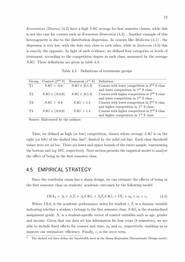
72

Economicas (Diurno) (4.2) have a high SAG average for first semester classes, while thisis not the case for courses such as Economia Domestica (4.3) . Another example of thisheterogeneity is due to the distribution dispersion. In courses like Medicina (4.1) , thedispersion is very low, with the dots very close to each other, while in Zootecnia (4.3) thisis exactly the opposite. In light of such evidence, we defined four categories or levels oftreatment, according to the competition degree in each class, measured by the averageSAG. These definitions are given in table 4.3.

Table 4.3 – Definitions of treatments groups

Group Control (2nd S) Treatment (1st S) DefinitionT1 SAG < -0.8 SAG ∈ [0,1.4] Courses with lower competition in 2nd S class

and lower competition in 1st S class.T2 SAG ∈ [-0.8,0) SAG ∈ [0,1.4] Courses with higher competition in 2nd S class

and lower competition in 1st S class.T3 SAG < -0.8 SAG > 1.4 Courses with lower competition in 2nd S class

and higher competition in 1st S class.T4 SAG ∈ [-0.8,0) SAG > 1.4 Courses with higher competition in 2nd S class

and higher competition in 1st S class.Source: Elaborated by the authors

Thus, we defined as high (or low) competition, classes whose average SAG is on theright (or left) of the dashed blue line5, limited by the solid red line. Each class thresholdvalues were set ad hoc. There are lower and upper bounds of the entire sample, representingthe bottom and top 10%, respectively. Next section presents the empirical model to analyzethe effect of being in the first semester class.

4.5 EMPIRICAL STRATEGYSince the vestibular exam has a sharp design, we can estimate the effects of being in

the first semester class on students’ academic outcomes by the following model:

IRAit = β0 + β1Ti + β2SAGi + β3TiSAGi + δXi + αk + αt + εi (4.2)

Where IRAi is the academic performance index for student i, Ti is a dummy variableindicating whether a student i belongs to the first semester class, SAGi is the standardizedassignment grade, Xi is a student-specific vector of control variables such as age, genderand income. Given that our data set has information for four years (8 semesters), we areable to include fixed effects for courses and time, αk and αt, respectively, enabling us toimprove our estimators’ efficiency. Finally, εi is the error term.5 The dashed red lines define the bandwidth used in the Sharp Regression Discontinuity Design model.

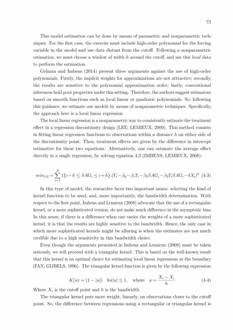
73

This model estimation can be done by means of parametric and nonparametric tech-niques. For the first case, the exercise must include high-order polynomial for the forcingvariable in the model and use data distant from the cutoff. Following a nonparametricestimation, we must choose a window of width h around the cutoff, and use this local datato perform the estimation.

Gelman and Imbens (2014) present three arguments against the use of high-orderpolynomials. Firstly, the implicit weights for approximations are not attractive; secondly,the results are sensitive to the polynomial approximation order; lastly, conventionalinferences hold poor properties under this setting. Therefore, the authors suggest estimatorsbased on smooth functions such as local linear or quadratic polynomials. So, followingthis guidance, we estimate our models by means of nonparametric techniques. Specifically,the approach here is a local linear regression.

The local linear regression is a nonparametric way to consistently estimate the treatmenteffect in a regression discontinuity design (LEE; LEMIEUX, 2009). This method consistsin fitting linear regression functions to observations within a distance h on either side ofthe discontinuity point. Then, treatment effects are given by the difference in interceptestimative for these two equations. Alternatively, one can estimate the average effectdirectly in a single regression, by solving equation 4.3 (IMBENS; LEMIEUX, 2008):

minβ,δ =N∑i=1

1{c−h ≤ SAGi ≤ c+h}.(Yi−β0−β1Ti−β2SAGi−β3TiSAGi−δXi)2 (4.3)

In this type of model, the researcher faces two important issues: selecting the kind ofkernel function to be used, and, more importantly, the bandwidth determination. Withrespect to the first point, Imbens and Lemieux (2008) advocate that the use of a rectangularkernel, or a more sophisticated version, do not make much difference in the asymptotic bias.In this sense, if there is a difference when one varies the weights of a more sophisticatedkernel, it is that the results are highly sensitive to the bandwidth. Hence, the only case inwhich more sophisticated kernels might be alluring is when the estimates are not muchcredible due to a high sensitivity in this bandwidth choice.

Even though the arguments presented in Imbens and Lemieux (2008) must be takenseriously, we will proceed with a triangular kernel. This is based on the well-known resultthat this kernel is an optimal choice for estimating local linear regressions at the boundary(FAN; GIJBELS, 1996). The triangular kernel function is given by the following expression:

K(u) = (1− |u|) for|u| ≤ 1, where u = Xi −Xc

h(4.4)

Where Xc is the cutoff point and h is the bandwidth.The triangular kernel puts more weight, linearly, on observations closer to the cutoff

point. So, the difference between regressions using a rectangular or triangular kernel is

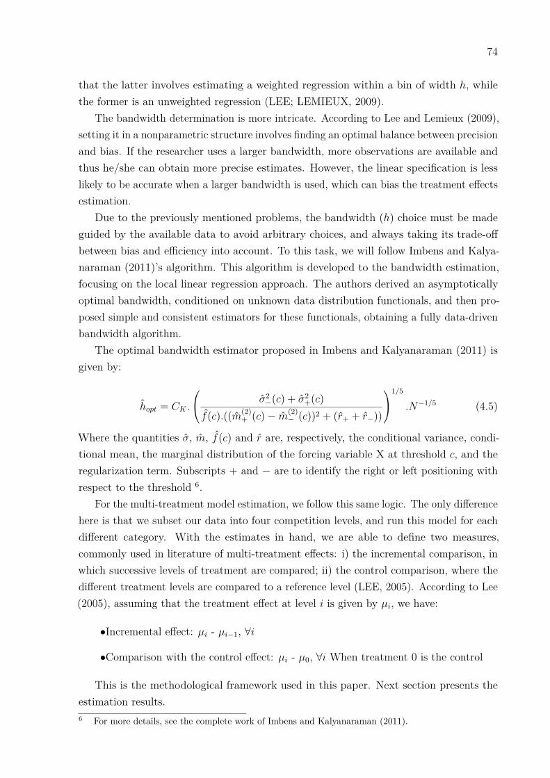
74

that the latter involves estimating a weighted regression within a bin of width h, whilethe former is an unweighted regression (LEE; LEMIEUX, 2009).

The bandwidth determination is more intricate. According to Lee and Lemieux (2009),setting it in a nonparametric structure involves finding an optimal balance between precisionand bias. If the researcher uses a larger bandwidth, more observations are available andthus he/she can obtain more precise estimates. However, the linear specification is lesslikely to be accurate when a larger bandwidth is used, which can bias the treatment effectsestimation.

Due to the previously mentioned problems, the bandwidth (h) choice must be madeguided by the available data to avoid arbitrary choices, and always taking its trade-offbetween bias and efficiency into account. To this task, we will follow Imbens and Kalya-naraman (2011)’s algorithm. This algorithm is developed to the bandwidth estimation,focusing on the local linear regression approach. The authors derived an asymptoticallyoptimal bandwidth, conditioned on unknown data distribution functionals, and then pro-posed simple and consistent estimators for these functionals, obtaining a fully data-drivenbandwidth algorithm.

The optimal bandwidth estimator proposed in Imbens and Kalyanaraman (2011) isgiven by:

hopt = CK .

σ2−(c) + σ2

+(c)f(c).((m(2)

+ (c)− m(2)− (c))2 + (r+ + r−))

1/5

.N−1/5 (4.5)

Where the quantities σ, m, f(c) and r are, respectively, the conditional variance, condi-tional mean, the marginal distribution of the forcing variable X at threshold c, and theregularization term. Subscripts + and − are to identify the right or left positioning withrespect to the threshold 6.

For the multi-treatment model estimation, we follow this same logic. The only differencehere is that we subset our data into four competition levels, and run this model for eachdifferent category. With the estimates in hand, we are able to define two measures,commonly used in literature of multi-treatment effects: i) the incremental comparison, inwhich successive levels of treatment are compared; ii) the control comparison, where thedifferent treatment levels are compared to a reference level (LEE, 2005). According to Lee(2005), assuming that the treatment effect at level i is given by µi, we have:

•Incremental effect: µi - µi−1, ∀i

•Comparison with the control effect: µi - µ0, ∀i When treatment 0 is the control

This is the methodological framework used in this paper. Next section presents theestimation results.6 For more details, see the complete work of Imbens and Kalyanaraman (2011).

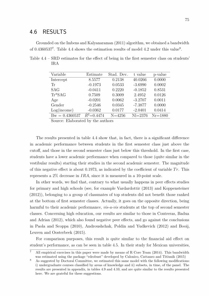
75

4.6 RESULTSGrounded on the Imbens and Kalyanaraman (2011) algorithm, we obtained a bandwidth

of 0.43605377. Table 4.4 shows the estimation results of model 4.2 under this value8.

Table 4.4 – SRD estimates for the effect of being in the first semester class on students’IRA

Variable Estimate Stad. Dev. t value p-valueIntercept 8.5577 0.2138 40.0266 0.0000Tr -0.1973 0.0533 -3.6990 0.0002SAG -0.0411 0.2220 -0.1852 0.8531Tr*SAG 0.7509 0.3009 2.4952 0.0126Age -0.0201 0.0062 -3.2707 0.0011Gender -0.2546 0.0345 -7.3877 0.0000Log(income) -0.0362 0.0177 -2.0401 0.0414Bw = 0.4360537 R2=0.4474 N=4256 Nl=2376 Nr=1880Source: Elaborated by the authors

The results presented in table 4.4 show that, in fact, there is a significant differencein academic performance between students in the first semester class just above thecutoff, and those in the second semester class just below this threshold. In the first case,students have a lower academic performance when compared to those (quite similar in thevestibular results) starting their studies in the second academic semester. The magnitudeof this negative effect is about 0.1973, as indicated by the coefficient of variable Tr. Thisrepresents a 2% decrease in IRA, since it is measured in a 10-point scale.

In other words, we find that, contrary to what usually happens in peer effects studiesfor primary and high schools (see, for example Vardardottir (2013) and Koppensteiner(2012)), belonging to a group of classmates of top students did not benefit those rankedat the bottom of first semester classes. Actually, it goes on the opposite direction, beingharmful to their academic performance, vis-a-vis students at the top of second semesterclasses. Concerning high education, our results are similar to those in Contreras, Baduaand Adrian (2012), which also found negative peer effects, and go against the conclusionsin Paola and Scoppa (2010), Androushchak, Poldin and Yudkevich (2012) and Booij,Leuven and Oosterbeek (2015).

For comparison purposes, this result is quite similar to the financial aid effect onstudent’s performance, as can be seen in table 4.5. In their study for Mexican universities,7 All empirical exercises in this paper were made by means of R Core Team (2014). This bandwidth

was estimated using the package “rdrobust” developed by Calonico, Cattaneo and Titiunik (2015)8 As suggested by Doctoral Committee, we estimated this same model with the following modifications:

i) undergraduate courses classified by areas of knowledge and ii) subsets, in time, of the panel. Theresults are presented in appendix, in tables 4.9 and 4.10, and are quite similar to the results presentedhere. We are grateful for these suggestions.

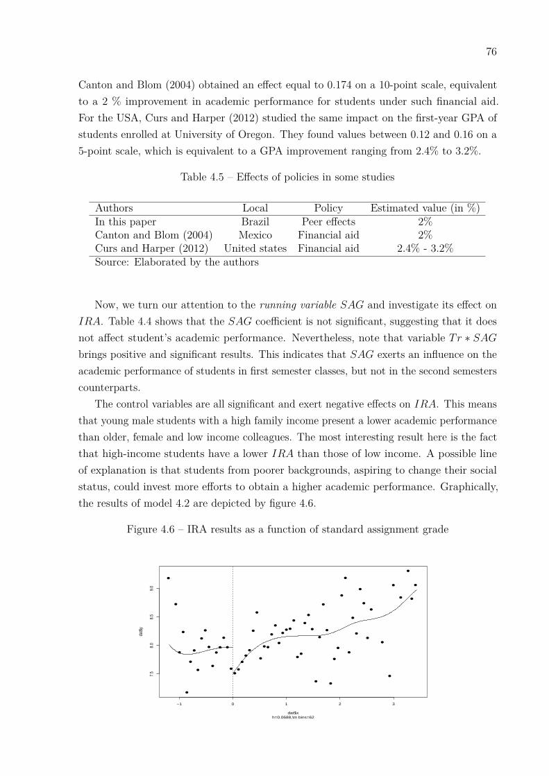
76

Canton and Blom (2004) obtained an effect equal to 0.174 on a 10-point scale, equivalentto a 2 % improvement in academic performance for students under such financial aid.For the USA, Curs and Harper (2012) studied the same impact on the first-year GPA ofstudents enrolled at University of Oregon. They found values between 0.12 and 0.16 on a5-point scale, which is equivalent to a GPA improvement ranging from 2.4% to 3.2%.

Table 4.5 – Effects of policies in some studies

Authors Local Policy Estimated value (in %)In this paper Brazil Peer effects 2%Canton and Blom (2004) Mexico Financial aid 2%Curs and Harper (2012) United states Financial aid 2.4% - 3.2%Source: Elaborated by the authors

Now, we turn our attention to the running variable SAG and investigate its effect onIRA. Table 4.4 shows that the SAG coefficient is not significant, suggesting that it doesnot affect student’s academic performance. Nevertheless, note that variable Tr ∗ SAGbrings positive and significant results. This indicates that SAG exerts an influence on theacademic performance of students in first semester classes, but not in the second semesterscounterparts.

The control variables are all significant and exert negative effects on IRA. This meansthat young male students with a high family income present a lower academic performancethan older, female and low income colleagues. The most interesting result here is the factthat high-income students have a lower IRA than those of low income. A possible lineof explanation is that students from poorer backgrounds, aspiring to change their socialstatus, could invest more efforts to obtain a higher academic performance. Graphically,the results of model 4.2 are depicted by figure 4.6.

Figure 4.6 – IRA results as a function of standard assignment grade

●

●

●

●

●

●

●

●

●

●

●

●

●

●

●

●

●

●

●

●

●

●

●

●

●

● ●

●

●

●

●

● ●

●

●

●

●

●

●

●

●

●

●

●

●

●

●

●

●

●

●

●

●

●

●

●

●

●

●

●

●

●

−1 0 1 2 3

7.5

8.0

8.5

9.0

dat$x

dat$

y

h=0.0688,\tn bins=62

77

We verified our results’ robustness to the bandwidth choice with a regression sensitivitytest. This test consists in reestimating model 4.2 using several bandwidths. After that,we plotted the relation between the bandwidth and the regression discontinuity design’sestimates, getting a visually powerful tool to explore the trade-off between bias andprecision (JACOB et al., 2012). This is presented in figure 4.7.

Figure 4.7 – Sensitivity test

●−0.2

0.0

0.2

0.4

0.6

0.0 0.5 1.0 1.5 2.0bw

LATE

This figure shows the treatment effects’ response to a bandwidth variation rangingfrom 0.01 to 2.18. As expected, for small bandwidth values, precision is low and bias ishigh, with the treatment effect being positive. As the bandwidth assumes higher values,bias decreases and precision increases, with the treatment effect turning negative. Forbandwidths larger than 0.5, the treatment effect is virtually unchanged, indicating thatours results are not much sensitive to the bandwidth choice near this value (rememberthat the optimal bandwidth is about 0.44).

The next step is to test the assignment variable’s continuity around the cutoff. A keyassumption in the regression discontinuity design approach is that agents are not able tomanipulate the assignment variable. If an individual can manipulate it, then he/she candecide whether or not to receive the treatment, so that continuity assumption may not beplausible. To test the this assignment variable’s continuity, we use the McCrary (2008)test.

From the McCrary (2008) test, we estimated a discontinuity around 0.10, with z−valueand p− value equal to 0.8875 and 0.3748, respectively. In this test, the null hypothesisis that the density is continuous around the cutoff. Given the choosen p − value, wecannot reject this null hypothesis, hence our assignment variable is really continuous9.The graphical result of this test is shown in figure 4.8.9 This result is not so surprising. Remember that students do not know the cutoff point, since it is

determined exogenously by competition. The only information in students’ possesion is the numberof vacancies. Therefore, we argue that if students do not know the cutoff, then they are not able tomanipulate the assignment variable

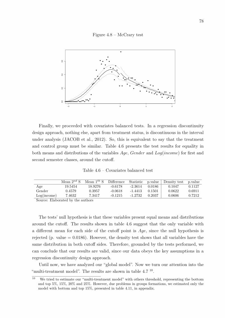
78

Figure 4.8 – McCrary test

−2 −1 0 1 2

0.0

0.2

0.4

0.6

● ● ● ● ●

●

● ● ● ● ● ● ● ● ● ● ●

●

● ●

● ●

●

● ●

●

●

●

●

●

●

●

●

●

●

●

●

●

●

●

●

●

●

●

●

●

●

●

●

●

●

●

●

● ●

●

●

●

● ●

●

●

● ●

●

●

●

●

● ●

●

●

●

●

●

●

●

●

●

●

●

●

●

●

● ●

●

●

●

●

●

●

●

●

● ●

Finally, we proceeded with covariates balanced tests. In a regression discontinuitydesign approach, nothing else, apart from treatment status, is discontinuous in the intervalunder analysis (JACOB et al., 2012). So, this is equivalent to say that the treatmentand control group must be similar. Table 4.6 presents the test results for equality inboth means and distributions of the variables Age, Gender and Log(income) for first andsecond semester classes, around the cutoff.

Table 4.6 – Covariates balanced test

Mean 2nd S Mean 1th S Difference Statistic p.value Density test p.valueAge 19.5454 18.9276 -0.6178 -2.3614 0.0186 0.1047 0.1127Gender 0.4579 0.3957 -0.0618 -1.4413 0.1501 0.0622 0.6911Log(income) 7.4632 7.3417 -0.1215 -1.2732 0.2037 0.0606 0.7212Source: Elaborated by the authors

The tests’ null hypothesis is that these variables present equal means and distributionsaround the cutoff. The results shown in table 4.6 suggest that the only variable witha different mean for each side of the cutoff point is Age, since the null hypothesis isrejected (p. value = 0.0186). However, the density test shows that all variables have thesame distribution in both cutoff sides. Therefore, grounded by the tests performed, wecan conclude that our results are valid, since our data obeys the key assumptions in aregression discontinuity design approach.

Until now, we have analyzed our “global model”. Now we turn our attention into the“multi-treatment model”. The results are shown in table 4.7 10.10 We tried to estimate our “multi-treatment model” with others threshold, representing the bottom

and top 5%, 15%, 20% and 25%. However, due problems in groups formations, we estimated only themodel with bottom and top 15%, presented in table 4.11, in appendix.

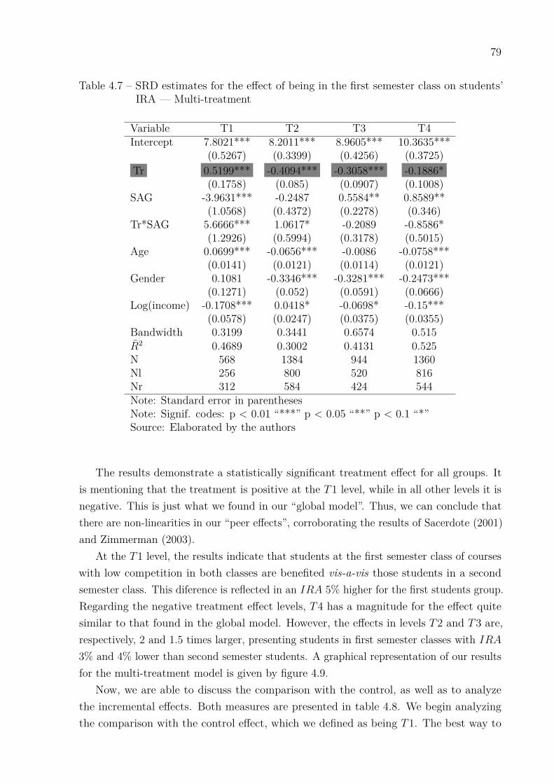
79

Table 4.7 – SRD estimates for the effect of being in the first semester class on students’IRA — Multi-treatment

Variable T1 T2 T3 T4Intercept 7.8021*** 8.2011*** 8.9605*** 10.3635***

(0.5267) (0.3399) (0.4256) (0.3725)Tr 0.5199*** -0.4094*** -0.3058*** -0.1886*

(0.1758) (0.085) (0.0907) (0.1008)SAG -3.9631*** -0.2487 0.5584** 0.8589**

(1.0568) (0.4372) (0.2278) (0.346)Tr*SAG 5.6666*** 1.0617* -0.2089 -0.8586*

(1.2926) (0.5994) (0.3178) (0.5015)Age 0.0699*** -0.0656*** -0.0086 -0.0758***

(0.0141) (0.0121) (0.0114) (0.0121)Gender 0.1081 -0.3346*** -0.3281*** -0.2473***

(0.1271) (0.052) (0.0591) (0.0666)Log(income) -0.1708*** 0.0418* -0.0698* -0.15***

(0.0578) (0.0247) (0.0375) (0.0355)Bandwidth 0.3199 0.3441 0.6574 0.515R2 0.4689 0.3002 0.4131 0.525N 568 1384 944 1360Nl 256 800 520 816Nr 312 584 424 544Note: Standard error in parenthesesNote: Signif. codes: p < 0.01 “***” p < 0.05 “**” p < 0.1 “*”Source: Elaborated by the authors

The results demonstrate a statistically significant treatment effect for all groups. Itis mentioning that the treatment is positive at the T1 level, while in all other levels it isnegative. This is just what we found in our “global model”. Thus, we can conclude thatthere are non-linearities in our “peer effects”, corroborating the results of Sacerdote (2001)and Zimmerman (2003).

At the T1 level, the results indicate that students at the first semester class of courseswith low competition in both classes are benefited vis-a-vis those students in a secondsemester class. This diference is reflected in an IRA 5% higher for the first students group.Regarding the negative treatment effect levels, T4 has a magnitude for the effect quitesimilar to that found in the global model. However, the effects in levels T2 and T3 are,respectively, 2 and 1.5 times larger, presenting students in first semester classes with IRA3% and 4% lower than second semester students. A graphical representation of our resultsfor the multi-treatment model is given by figure 4.9.

Now, we are able to discuss the comparison with the control, as well as to analyzethe incremental effects. Both measures are presented in table 4.8. We begin analyzingthe comparison with the control effect, which we defined as being T1. The best way to

80

Figure 4.9 – IRA results as a function of assignment grade

●

●

●

●

●●

●●

●

●

●●

●●

●●

●●

●

●

●

●

●

●

●

●

●●●

●

●

●

●

●

●

●

●

●

●

●

●●

●

●

●●

●

●

●

●●

●

●

●

●

●

●

●

−3 −2 −1 0 1 2 3

67

89

Normalized assigment grade

IRA

Treatment effect Estimate: 0.5199 (0.1758)

h=0.064,\tn bins=58

●

●

●

●

●

●

●

●

●

●

●

●

●

●

●

●

●●

●

●

●

●

●

●

●

●●

●

●

●

●●●

●

●●

●

●

●

●

●

●

●

●

●

●

●

●

●

●

●

●

●

●

●

●

●

●

●

●

●

●

−1 0 1 2 3

7.5

8.0

8.5

9.0


IRA

Treatment effect Estimate: −0.4094 (0.085)

h=0.0688,\tn bins=62

●

●

●

●

●

● ●

●●

●

●

●

●

●

●●

●

●

●

●

●

●

●●

●

●

●

● ●

●

●

●

●

−2 0 2

7.0

7.5

8.0

8.5

9.0

9.5


IRA


h=0.1315,\tn bins=33

●

●

●

●

●

●

●

●

●●

●●

●

●

● ●

● ●

●

●●

●

●

●

●

●

●

●

●

●

●

●

● ●

●

●

●

●

●

●

●

●

●

●

●●

●

−1 0 1 2 3 4 5

6.5

7.0

7.5

8.0

8.5

9.0

9.5


IRA


h=0.103,\tn bins=47

understand this is by thinking about a first-semester student. T1 has both classes withlow competition and a positive treatment effect. T2 has the first semester class associatedto a high competition and, thus, the student’s loss is 0.9292, compared to T1. In T3, thefirst semester class continues to be of low competition, but that of the second semester isa high competition class now. In this case, the students’ loss is less than in T2. Finally, inT4, both classes are of high competition, and the students’ loss is 0.7085, i.e., less than inT2 and T3.

Now, we are going to analyze the treatment’s incremental effect following the samelogic as previously. The change from T1 to T2 is already analyzed. When the treatmentof a first-semester student is initially T2, and changes to T3, his/her class becomes oflow competition, and high competition is associated with the second semester class. Inthe case of a change from T3 to T4, both classes are of high competition now. In bothchanges, there is no significant effect.

Therefore, we can conclude that the peer effects are positive when both classes are oflow competition, and negative in the other cases. However, note that this negative effectis lower when both classes are of high competition. In addition, the incremental effect issignificant only when first and second semester classes present high and low competition,respectively.

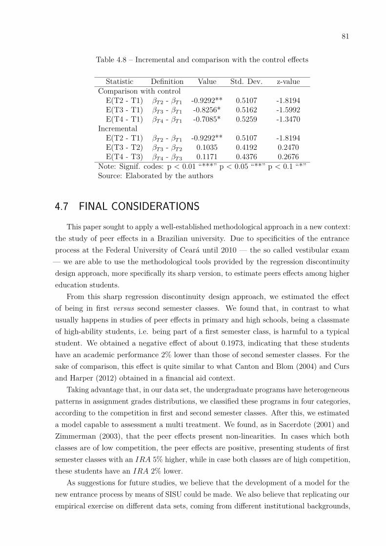
81

Table 4.8 – Incremental and comparison with the control effects

Statistic Definition Value Std. Dev. z-valueComparison with control

E(T2 - T1) βT2 - βT1 -0.9292** 0.5107 -1.8194E(T3 - T1) βT3 - βT1 -0.8256* 0.5162 -1.5992E(T4 - T1) βT4 - βT1 -0.7085* 0.5259 -1.3470

IncrementalE(T2 - T1) βT2 - βT1 -0.9292** 0.5107 -1.8194E(T3 - T2) βT3 - βT2 0.1035 0.4192 0.2470E(T4 - T3) βT4 - βT3 0.1171 0.4376 0.2676

Note: Signif. codes: p < 0.01 “***” p < 0.05 “**” p < 0.1 “*”Source: Elaborated by the authors

4.7 FINAL CONSIDERATIONSThis paper sought to apply a well-established methodological approach in a new context:

the study of peer effects in a Brazilian university. Due to specificities of the entranceprocess at the Federal University of Ceará until 2010 — the so called vestibular exam— we are able to use the methodological tools provided by the regression discontinuitydesign approach, more specifically its sharp version, to estimate peers effects among highereducation students.

From this sharp regression discontinuity design approach, we estimated the effectof being in first versus second semester classes. We found that, in contrast to whatusually happens in studies of peer effects in primary and high schools, being a classmateof high-ability students, i.e. being part of a first semester class, is harmful to a typicalstudent. We obtained a negative effect of about 0.1973, indicating that these studentshave an academic performance 2% lower than those of second semester classes. For thesake of comparison, this effect is quite similar to what Canton and Blom (2004) and Cursand Harper (2012) obtained in a financial aid context.

Taking advantage that, in our data set, the undergraduate programs have heterogeneouspatterns in assignment grades distributions, we classified these programs in four categories,according to the competition in first and second semester classes. After this, we estimateda model capable to assessment a multi treatment. We found, as in Sacerdote (2001) andZimmerman (2003), that the peer effects present non-linearities. In cases which bothclasses are of low competition, the peer effects are positive, presenting students of firstsemester classes with an IRA 5% higher, while in case both classes are of high competition,these students have an IRA 2% lower.

As suggestions for future studies, we believe that the development of a model for thenew entrance process by means of SISU could be made. We also believe that replicating ourempirical exercise on different data sets, coming from different institutional backgrounds,

82

might be something worth pursuing to validate our approach. Finally, we believe that thisshould be done with ENADE’s 11score as an outcome, instead of IRA′s. It would help usto understand this effect better.

11 The National Survey of Students’ Performance (ENADE) is an exam that constitutes the NationalSystem of Higher Education Assessment (Sinaes). This test aims to assess students’ performance inrelation to the syllabus provided in the curriculum guidelines of their undergraduate programs, andthe skills and competences in their training ((INEP), 2015).

REFERENCES

ABDULKADIROĞLU, A.; ANGRIST, J.; PATHAK, P. The elite illusion: Achievementeffects at boston and new york exam schools. Econometrica, Wiley Online Library, v. 82,n. 1, p. 137–196, 2014.

ABREU, L. C. M. Mecanismos de seleção Gale-Shapley dinâmicos em universidadesBrasileiras: SISU , SISUalpha, SISUbeta. Dissertação (Dissertação de mestrado) —Universidade Federal do Ceará, 2013.

ANDROUSHCHAK, G. V.; POLDIN, O.; YUDKEVICH, M. Peer effects in exogenouslyformed university student groups. [S.l.], 2012. v. 3, n. 03/EDU/2012.

BOOIJ, A.; LEUVEN, E.; OOSTERBEEK, H. Ability peer effects in university: Evidencefrom a randomized experiment. [S.l.], January 2015.

BUTCHER, K. F.; MCEWAN, P. J.; TAYLOR, C. H. The effects of quantitative skillstraining on college outcomes and peers. Economics of Education Review, Elsevier, v. 29,n. 2, p. 187–199, 2010.

CALONICO, S.; CATTANEO, M. D.; TITIUNIK, R. rdrobust: Robust Data-DrivenStatistical Inference in Regression-Discontinuity Designs. [S.l.], 2015. R package version0.80. Disponível em: <http://CRAN.R-project.org/package=rdrobust>.

CANTON, E.; BLOM, A. Do student loans improve accessibility to higher education andstudent performance. [S.l.]: CPB Netherlands Bureau for Economic Policy Analysis TheHague, 2004.

CARD, d.; GIULIANO, L. Can tracking raise the test scores of high-abilitybility minoritystudents? March 2015.

CARRELL, S. E.; FULLERTON, R. L.; WEST, J. E. Does your cohort matter?Measuring peer effects in college achievement. [S.l.], 2008.

CARVALHO, J.-R.; MAGNAC, T.; XIONG, Q. College Choice Allocation Mechanisms:Structural Estimates and Counterfactuals. [S.l.], June 2014.

CEARÁ FEDERAL UNIVERSITY. UFC statistical yearbook - A brief edition2013-2014. 2014. Disponível em: <http://www.ufc.br/images/ files/a universidade-/anuario estatistico/statistical yearbook ufc 2014 2013.pdf>.

COLEMAN, J. S. et al. Equality of educational opportunity. Washington, dc, p. 1066–5684,1966.

http://CRAN.R-project.org/package=rdrobust

http://www.ufc.br/images/_files/a_universidade/anuario_estatistico/statistical_yearbook_ufc_2014_2013.pdf

http://www.ufc.br/images/_files/a_universidade/anuario_estatistico/statistical_yearbook_ufc_2014_2013.pdf

84

CONTRERAS, S.; BADUA, F.; ADRIAN, M. Peer effects on undergraduate businessstudent performance. International Review of Economic Education, Economics Network,University of Bristol, v. 11, n. 1, p. 57–66, 2012.

CURS, B. R.; HARPER, C. E. Financial aid and first-year collegiate gpa: A regressiondiscontinuity approach. The Review of Higher Education, The Johns Hopkins UniversityPress, v. 35, n. 4, p. 627–649, 2012.

EPPLE, D.; ROMANO, R. Peer effects in education: A survey of the theory and evidence.Handbook of social economics, Forthcoming, v. 1, n. 11, p. 1053–1163, 2011.

FAN, J.; GIJBELS, I. Local polynomial modelling and its applications: Monographs onstatistics and applied probability 66. Taylor and Francis, 1996. (Chapman & Hall/CRCMonographs on Statistics & Applied Probability). ISBN 9780412983214. Disponível em:<https://books.google.com.br/books?id=BM1ckQKCXP8C>.

GAWANDE, A. BrainyQuote.com. n.d. <http://www.brainyquote.com/quotes/quotes/a/atulgawand527239.html>. Accessed: May 22, 2015.

GELMAN, A.; IMBENS, G. Why high-order polynomials should not be used in regressiondiscontinuity designs. [S.l.], 2014.

IMBENS, G.; KALYANARAMAN, K. Optimal bandwidth choice for the regressiondiscontinuity estimator. The Review of Economic Studies, Oxford University Press, v. 79,n. 3, p. 933–959, 2011.

IMBENS, G. W.; LEMIEUX, T. Regression discontinuity designs: A guide to practice.Journal of econometrics, Elsevier, v. 142, n. 2, p. 615–635, 2008.

(INEP), I. de Estudos e P. E. A. T. Censo da educação superior 2013. 2014. Disponívelem: <http://download.inep.gov.br/educacao superior/censo superior/apresentacao-/2014/coletiva censo superior 2013.pdf>.

(INEP), I. de Estudos e P. E. A. T. Exame Nacional de Desempenho de Estudantes -ENADE. May 2015. Disponível em: <http://portal.inep.gov.br/enade>.

JACOB, R. T. et al. A practical guide to regression discontinuity. [S.l.]: MDRC, 2012.

KLAAUW, W. Van der. Estimating the effect of financial aid offers on college enrollment:A regression discontinuity approach. International Economic Review, Wiley OnlineLibrary, v. 43, n. 4, p. 1249–1287, 2002.

KOPPENSTEINER, M. F. Class assignment and peer group effects: Evidence fromBrazilian primary schools. [S.l.], 2012.

LEE, D. S.; LEMIEUX, T. Regression discontinuity designs in economics. [S.l.], 2009.

http://www.brainyquote.com/quotes/quotes/a/atulgawand527239.html

http://www.brainyquote.com/quotes/quotes/a/atulgawand527239.html

http://download.inep.gov.br/educacao_superior/censo_superior/apresentacao/2014/coletiva_censo_superior_2013.pdf

http://download.inep.gov.br/educacao_superior/censo_superior/apresentacao/2014/coletiva_censo_superior_2013.pdf

http://portal.inep.gov.br/enade

85

LEE, M.-J. Micro-econometrics for policy, program, and treatment effects. [S.l.]: OxfordUniversity Press Oxford, 2005.

LEEDS, D. M.; DESJARDINS, S. L. The effect of merit aid on enrollment: A regressiondiscontinuity analysis of iowa’s national scholars award. Research in Higher Education,Springer, p. 1–25, 2014.

MANSKI, C. F. Identification of endogenous social effects: The reflection problem. Thereview of economic studies, Oxford University Press, v. 60, n. 3, p. 531–542, 1993.

MCCRARY, J. Manipulation of the running variable in the regression discontinuitydesign: A density test. Journal of Econometrics, Elsevier, v. 142, n. 2, p. 698–714, 2008.

MCEWAN, P. J.; SODERBERG, K. A. Roommate effects on grades: Evidence fromfirst-year housing assignments. Research in Higher Education, Springer, v. 47, n. 3, p.347–370, 2006.

MEALLI, F.; RAMPICHINI, C. Evaluating the effects of university grants by usingregression discontinuity designs. Journal of the Royal Statistical Society: Series A(Statistics in Society), Wiley Online Library, v. 175, n. 3, p. 775–798, 2012.

MOSS, B. G.; YEATON, W. H. Shaping policies related to developmental education: Anevaluation using the regression-discontinuity design. Educational Evaluation and PolicyAnalysis, Sage Publications, v. 28, n. 3, p. 215–229, 2006.

PAOLA, M. D.; SCOPPA, V. Peer group effects on the academic performance of italianstudents. Applied Economics, Taylor & Francis, v. 42, n. 17, p. 2203–2215, 2010.

R Core Team. R: A Language and Environment for Statistical Computing. Vienna,Austria, 2014. Disponível em: <http://www.R-project.org/>.

SACERDOTE, B. Peer effects with random assignment: Results for dartmouthroommates. The Quarterly Journal of Economics, Oxford University Press (OUP), v. 116,n. 2, p. 681–704, May 2001. ISSN 1531-4650. Disponível em: <http://dx.doi.org/10.1162-/00335530151144131>.

SACERDOTE, B. Peer effects in education: How might they work, how big are they andhow much do we know thus far? Handbook of the Economics of Education, Elsevier, v. 3,p. 249–277, 2011.

SCHÖER, V.; SHEPHERD, D. Compulsory tutorial programmes and performance inundergraduate microeconomics: A regression discontinuity design. [S.l.], September 2013.

SILVA, J. E. M. d. Vestibular na UFC: Implicações para o ensino médio — Um estudode caso a partir das mudanças realizadas de 1978 a 2004. Dissertação (Dissertação demestrado) — Universidade Federal do Ceará, 2007.

http://www.R-project.org/

http://dx.doi.org/10.1162/00335530151144131

http://dx.doi.org/10.1162/00335530151144131

86

VARDARDOTTIR, A. Peer effects and academic achievement: A regression discontinuityapproach. Economics of Education Review, Elsevier, v. 36, p. 108–121, 2013.

WINSTON, G.; ZIMMERMAN, D. Peer effects in higher education. In: College choices:The economics of where to go, when to go, and how to pay for it. [S.l.]: University ofChicago Press, 2004. p. 395–424.

ZIMMERMAN, D. J. Peer effects in academic outcomes: Evidence from a naturalexperiment. Review of Economics and Statistics, MIT Press, v. 85, n. 1, p. 9–23, 2003.

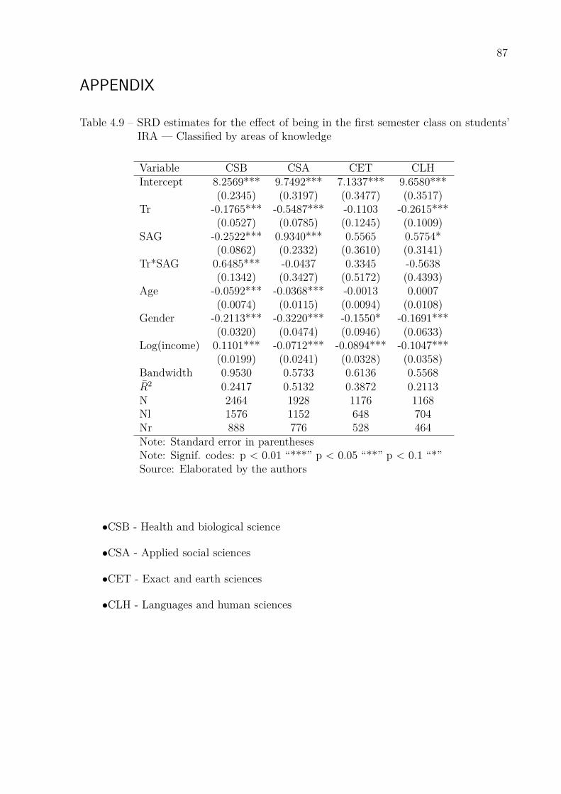
87

APPENDIX

Table 4.9 – SRD estimates for the effect of being in the first semester class on students’IRA — Classified by areas of knowledge

Variable CSB CSA CET CLHIntercept 8.2569*** 9.7492*** 7.1337*** 9.6580***

(0.2345) (0.3197) (0.3477) (0.3517)Tr -0.1765*** -0.5487*** -0.1103 -0.2615***

(0.0527) (0.0785) (0.1245) (0.1009)SAG -0.2522*** 0.9340*** 0.5565 0.5754*

(0.0862) (0.2332) (0.3610) (0.3141)Tr*SAG 0.6485*** -0.0437 0.3345 -0.5638

(0.1342) (0.3427) (0.5172) (0.4393)Age -0.0592*** -0.0368*** -0.0013 0.0007

(0.0074) (0.0115) (0.0094) (0.0108)Gender -0.2113*** -0.3220*** -0.1550* -0.1691***

(0.0320) (0.0474) (0.0946) (0.0633)Log(income) 0.1101*** -0.0712*** -0.0894*** -0.1047***


•CSB - Health and biological science

•CSA - Applied social sciences

•CET - Exact and earth sciences

•CLH - Languages and human sciences

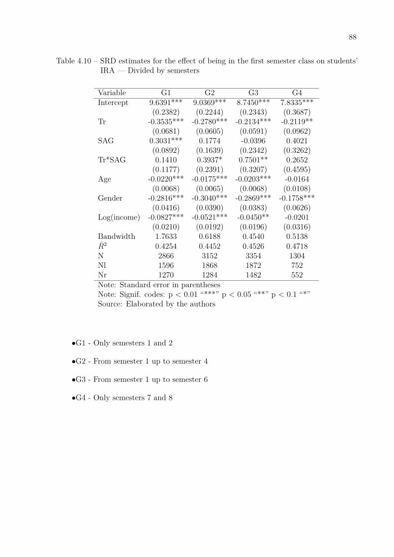
88

Table 4.10 – SRD estimates for the effect of being in the first semester class on students’IRA — Divided by semesters

Variable G1 G2 G3 G4Intercept 9.6391*** 9.0369*** 8.7450*** 7.8335***

(0.2382) (0.2244) (0.2343) (0.3687)Tr -0.3535*** -0.2780*** -0.2134*** -0.2119**

(0.0681) (0.0605) (0.0591) (0.0962)SAG 0.3031*** 0.1774 -0.0396 0.4021

(0.0892) (0.1639) (0.2342) (0.3262)Tr*SAG 0.1410 0.3937* 0.7501** 0.2652

(0.1177) (0.2391) (0.3207) (0.4595)Age -0.0220*** -0.0175*** -0.0203*** -0.0164

(0.0068) (0.0065) (0.0068) (0.0108)Gender -0.2816*** -0.3040*** -0.2869*** -0.1758***

(0.0416) (0.0390) (0.0383) (0.0626)Log(income) -0.0827*** -0.0521*** -0.0450** -0.0201


•G1 - Only semesters 1 and 2

•G2 - From semester 1 up to semester 4

•G3 - From semester 1 up to semester 6

•G4 - Only semesters 7 and 8

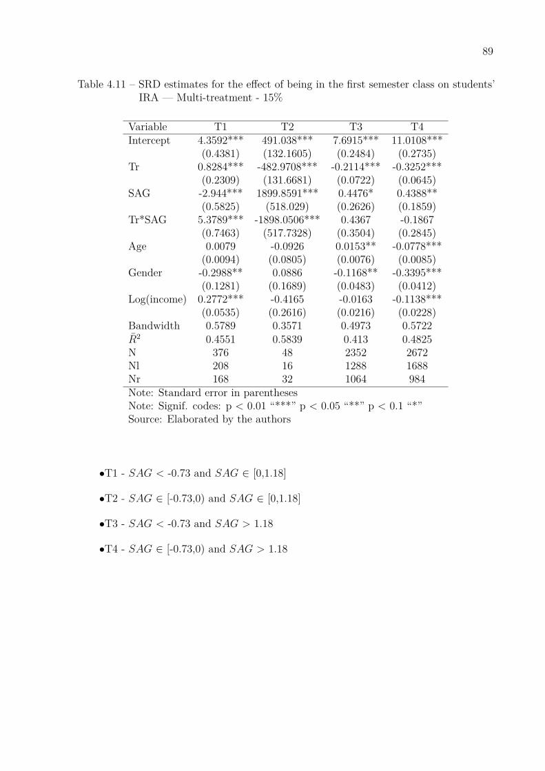
89

Table 4.11 – SRD estimates for the effect of being in the first semester class on students’IRA — Multi-treatment - 15%

Variable T1 T2 T3 T4Intercept 4.3592*** 491.038*** 7.6915*** 11.0108***

(0.4381) (132.1605) (0.2484) (0.2735)Tr 0.8284*** -482.9708*** -0.2114*** -0.3252***

(0.2309) (131.6681) (0.0722) (0.0645)SAG -2.944*** 1899.8591*** 0.4476* 0.4388**

(0.5825) (518.029) (0.2626) (0.1859)Tr*SAG 5.3789*** -1898.0506*** 0.4367 -0.1867

(0.7463) (517.7328) (0.3504) (0.2845)Age 0.0079 -0.0926 0.0153** -0.0778***

(0.0094) (0.0805) (0.0076) (0.0085)Gender -0.2988** 0.0886 -0.1168** -0.3395***

(0.1281) (0.1689) (0.0483) (0.0412)Log(income) 0.2772*** -0.4165 -0.0163 -0.1138***


•T1 - SAG < -0.73 and SAG ∈ [0,1.18]

•T2 - SAG ∈ [-0.73,0) and SAG ∈ [0,1.18]

•T3 - SAG < -0.73 and SAG > 1.18

•T4 - SAG ∈ [-0.73,0) and SAG > 1.18

APPENDICES

UNIVERSIDADE FEDERAL DO CEARÁ FACULDADE DE …©.pdf · universidade federal do cearÁ faculdade...

Documents

Transcript of UNIVERSIDADE FEDERAL DO CEARÁ FACULDADE DE …©.pdf · universidade federal do cearÁ faculdade...