Universidad Complutense de Madrid Facultad de Ciencias ... · Universidad Complutense de Madrid...

Universidad Complutense de Madrid

Facultad de Ciencias Matematicas

Proyecto Fin de Master en Investigacion MatematicaAcademic Year: 2008-2009

On the stability of vector bundles

Alfonso Zamora Saiz∗

Directed by Ignacio Sols

Supervised by Tomas Luis Gomez

∗The author was supported by a FPU fellowship from the Spanish Ministry of

Education

El abajo firmante, matriculado en el Master en Investigacion Matematica de la

Facultad de Ciencias Matematicas, autoriza a la Universidad Complutense de Madrid

(UCM) a difundir y utilizar con fines academicos, no comerciales y mencionando ex-

presamente a su autor, el presente Trabajo de Fin de Master: “On the stability of

vector bundles”, realizado durante el curso academico 2008-2009 bajo la direccion del

profesor Ignacio Sols y con la colaboracion del profesor Tomas Luis Gomez (CSIC),

y a la Biblioteca de la UCM a depositarlo en el Archivo Institucional E-Prints Com-

plutense con el objeto de incrementar la difusion, uso e impacto del trabajo en Internet

y garantizar su preservacion y acceso a largo plazo.

Alfonso Zamora Saiz

i

Abstract

In this work we present vector bundles and their properties. We will expose the

construction of the moduli space of vector bundles on a smooth projective algebraic

curve, following Gieseker´s construction, as a way of classifying them. We will talk

about the notion of stability which let us make a construction for the semistable

bundles and we will give some ideas about Geometric Invariant Theory, one-parameter

subgroups, and their contributions to our problem. Afterwards, we give the Harder-

Narashiman filtration for unstable vector bundles. Finally, we consider the Kempf’s

one-parameter subgroup, as the best way of destabilizing for an unstable point and

we apply it to the case of vector bundles to obtain a destabilizing filtration. The main

result of the work is to conclude that the Kempf filtration and the Harder-Narashiman

filtration are really the same.

Mathematical Subject Classification (2010): primary 14H60; secondary 14D20.

Key words: moduli space, vector bundles, algebraic curves, Geometric Invariant

Theory, Harder-Narasimhan filtration, Kempf one-parametric subgroup

ii

Resumen

En este trabajo presentamos los fibrados vectoriales y sus propiedades. Expondremos

la construccion del espacio de moduli de fibrados vectoriales sobre una curva alge-

braica proyectiva no singular, siguiendo la construccion de Gieseker, como forma

de clasificarlos. Hablaremos acerca de la nocion de estabilidad que nos permite re-

alizar una construccion para los fibrados semiestables y daremos algunas ideas acerca

de la Teorıa de Invariantes Geometricos, los subgrupos uniparametricos, y sus con-

tribuciones a nuestro problema. Despues, damos la filtracion de Harder-Narasimhan

para los fibrados vectoriales inestables. Finalmente, consideramos el subgrupo uni-

parametrico de Kempf, como la mejor forma de desestabilizar un punto inestable y lo

aplicamos al caso de fibrados vectoriales para obtener una filtracion desestabilizante.

El principal resultado del trabajo es concluir que la filtracion de Kempf y la filtracion

de Harder-Narasimhan son realmente la misma.

Mathematical Subject Classification (2010): primaria 14H60; secundaria 14D20.

Palabras clave: espacio de moduli, fibrados vectoriales, curvas algebraicas, Teorıa

de Invariantes Geometricos, filtracion de Harder-Narasimhan, subgrupo uniparametrico

de Kempf

Contents

Abstract . . . . . . . . . . . . . . . . . . . . . . . . . . . . . . . . . . . . . i

Resumen . . . . . . . . . . . . . . . . . . . . . . . . . . . . . . . . . . . . . ii

Contents iii

Introduction 1

1 Background 4

1.1 Sheaves . . . . . . . . . . . . . . . . . . . . . . . . . . . . . . . . . . 5

1.2 Vector bundles . . . . . . . . . . . . . . . . . . . . . . . . . . . . . . 7

1.3 Degree of a vector bundle . . . . . . . . . . . . . . . . . . . . . . . . 9

2 The moduli space of vector bundles 12

2.1 The concept of moduli . . . . . . . . . . . . . . . . . . . . . . . . . . 12

2.2 Gieseker construction of the moduli space of vector bundles . . . . . . 14

2.3 Geometric Invariant Theory . . . . . . . . . . . . . . . . . . . . . . . 19

iii

iv

2.4 One-parameter subgroups . . . . . . . . . . . . . . . . . . . . . . . . 23

2.5 Application of GIT to the construction of the moduli space . . . . . . 26

3 The Harder-Narasimhan filtration 28

4 The Kempf filtration 32

4.1 Convex cones . . . . . . . . . . . . . . . . . . . . . . . . . . . . . . . 33

4.2 The m-Kempf filtration of an unstable bundle . . . . . . . . . . . . . 36

4.3 Properties of the m-Kempf filtration of E . . . . . . . . . . . . . . . . 40

4.4 The Kempf filtration is the Harder-Narasimhan filtration . . . . . . . 44

A Simpson construction of the moduli space 46

Bibliography 47

Introduction

Vector bundles are an important object of study. They make precise the idea of a

family of vector spaces parametrized by another space, which can be a topological

space, a differential manifold, an algebraic variety, etc. In algebraic geometry, they

are used to provide functions over algebraic varieties. A complex projective algebraic

variety is a compact topological space, thus its global functions to the complex field

are only the constants. Then, vector bundles provide us global sections -meromorphic

functions- over algebraic varieties, apart from the global functions. Knowing whether

a vector bundle has global sections or not and, in the affirmative case, computing the

dimension of the space of global sections, is precisely knowing the dimension of the

vector space of global functions the vector bundle defines over our variety.

In fact, vector bundles are a particular case of a more general construction, prin-

cipal bundles (where the transition functions map in a group G, in general different

from the general linear group). Principal bundles have important applications in

topology, differential geometry and gauge theories in physics. They provide a unify-

ing framework for the theory of fiber bundles in the sense that all fiber bundles with

structure group G determine a unique principal G-bundle from which the original

bundle can be reconstructed.

There are two main purposes in this report. The first one is to study vector

bundles. The second one is to pave the way for the study of tensors, which are vector

bundles with additional structure.

Dealing with vector bundles, beyond the background of the framework given in

Chapter 1, we encounter the idea of moduli. In mathematics, to study something is,

1

2

in one way or another, to classify the objects we are working with. And this is the idea

of what a moduli space is: a good way of parametrizing a family of objects, meaning

that the moduli space has a good structure (it will be an algebraic variety) and that

isomorphism classes of objects correspond with points of it. We will construct a

moduli space for vector bundles over a given curve, with their algebraic invariants

fixed, degree, rank and genus.

The first construction was due to Mumford, who gave the moduli space for stable

sheaves over algebraic curves. The next was the construction of Narashiman and

Seshadri for semistable sheaves over curves, with which we get the compactness of

the moduli space. Gieseker and Maruyama extended it to the case of an algebraic

variety higher dimension and later, Simpson gave another method to do it. The

last result of Adrian Langer obtains a moduli space for semistable sheaves over an

algebraic variety of dimension n, in characteristic p. The difficulty in higher dimension

is to prove the boundedness of semistable sheaves.

Here we are going to follow the construction of the moduli space of semistable

vector bundles over curves due to David Gieseker. To complete, in some way, the

classification, we use the filtration given by Harder and Narasimhan. This filtration

characterizes the unstable vector bundles and it is the best way to destabilize them.

In order to study the semistable vector bundles, as well as the unstable ones,

we use the powerful machinery of the Geometric Invariant Theory, due to Mumford.

This framework appears in the heart of many problems in geometry. In our case, it

gives numerical criteria to determine the type of the bundle through one-parameter

subgroups, which can destabilize or not.

In the unstable case some one-parameter subgroups turn out to be better than

others. And this was the inspiration of George Kempf: the fact that there exists a

way to destabilize a unstable object which is the best one. The main purpose of this

work is to prove that the Harder-Narasimhan filtration and the Kempf filtration (the

filtration provided by the one-parameter subgroup defined in Kempf’s article) are the

same. Both of them are the best way to destabilize a unstable vector bundle.

In the case of tensors there have been several attempts at giving a similar desta-

3

bilizing filtration. The stability for tensors depends on a parameter which relates

the vector bundle and the additional information (a morphism). We cannot obtain a

maximum destabilizing object because it can destabilize the vector bundle or the mor-

phism but not both at the same time. The aim is to use the Kempf’s one-parameter

subgroup to give the best way of destabilizing for tensors.

There are very important theorems of Mehta and Ramanathan on the restriction

of a semistable vector bundle from a variety to a subvariety. However, they are proved

only in the case of sheaves. Being able to give a Kempf filtration in the case of tensors

would definitely help in order to extend these results.

Chapter 1

Background

In this section we present the concepts and properties that we are going to need in this

work. We want to emphasize that the theory and most of the general results are stated

in the framework of schemes. To deal with schemes is more difficult because they

represent the natural generalization of algebraic varieties but with a very technical

language. Given that the main argument can be followed substituting scheme for

algebraic variety we have preferred to take the easier way. Similarly we have omitted

several considerations about sheaf cohomology and Chern classes. For a complete

treatment of schemes and cohomology of sheaves, see [Ha].

We give the basic definitions about sheaves over algebraic curves. We present

vector bundles and their connection with classes of Cech cohomology, and we discuss

the definition of the degree of a vector bundle. For all of this, we suppose the reader

to be familiarized with algebraic varieties.

In this work X will be a smooth projective algebraic variety of dimension 1 over

C, which is the same that a Riemann surface. We call it algebraic curve or just curve.

4

CHAPTER 1. BACKGROUND 5

1.1 Sheaves

Definition 1.1.1. A presheaf F of abelian groups (resp. rings, modules...) over a

topological space X consists of the data

• for every open subset U ⊂ X, an abelian group F(U)

• for every inclusion V ⊂ U of open subsets of X, a morphism of abelian groups

ρUV : F(U)→ F(V ), subject to the conditions

1. F(∅) = 0, where ∅ is the empty set

2. ρUU : F(U)→ F(U) is the identity map

3. if W ⊂ V ⊂ U are three open subsets, then ρUW = ρVW ◦ ρUV

We define a presheaf of rings, modules, etc..., by replacing the words ”abelian

group” in the definition by ”ring”, ”module”, etc.

If F is a presheaf on X, we refer to s ∈ F(U) as the sections of the presheaf Fover the open set U , and we use the notation Γ(U,F) to denote the group F(U). We

call the maps ρUV restriction maps, and we sometimes write s|V instead of ρUV (s), if

s ∈ F(U).

Remark 1.1.2. If we consider, for any topological space X, the category Top(X),

whose objects are the open subsets of X, and where the only morphisms are the in-

clusion maps, a presheaf is just a contravariant functor from the category Top(X) to

the category Ab of abelian groups.

Definition 1.1.3. A presheaf F over a topological space X is a sheaf if it satisfies

the following supplementary conditions:

4. if U is an open set, if {Vi} is an open covering of U , and if s ∈ F(U) is an

element such that s|Vi = 0 for all i, then s = 0

5. if U is an open set, if {Vi} is an open covering of U, and if we have elements

si ∈ F(Vi) for each i, with the property that for each i, j, si|Vi∩Vj = sj|Vi∩Vj ,then there is an element s ∈ F(U) such that s|Vi = si for each i


(Note that condition (4.) implies that s is unique).

Definition 1.1.4. If F is a presheaf over X, and if P is a point of X, we define

the stalk FP of F at P to be the direct limit of the groups F(U) for all open sets U

containing P , via the restriction maps ρ.

Given a sheaf of rings A on X we can consider a sheaf of modules F over the

sheaf of rings A in such a way that on each open set U ⊂ X, F(U) is a module over

the ring A(U) and the restriction homomorphisms agree with the module structure.

The sheaf F is said to be a sheaf of A-modules.

Definition 1.1.5. Let A be a sheaf of rings on X. A sheaf of A-modules, F , is free

if F ' Ar, for any r. F is locally free if there exists a covering of {Ui} of X such

that F|Ui ' Ar|Ui, for any r.

Definition 1.1.6. Let F be a sheaf over X. The support of F , denoted SuppF , is

defined to be {P ∈ X : FP 6= 0}, where FP is the stalk of F at P .

Definition 1.1.7. A sheaf F of A-modules is a torsion sheaf if for each open set

U ⊂ X and for all s ∈ F(U), s is a torsion element (m 6= 0 is a torsion element of a

module M over a ring A if there exists an element a ∈ A, a 6= 0 such that a ·m = 0).

Definition 1.1.8. A sheaf F of A-modules is a torsion-free sheaf if for each open

set U ⊂ X the module F(U) has no torsion elements.

Definition 1.1.9. A sheaf F is pure if ∀F ′ ⊂ F , dim SuppF ′ = dim SuppF .

The intuitive idea of a pure sheaf is a sheaf which is torsion-free if we restrict it

to its support. Note that if F is torsion-free, then F is pure.

Remark 1.1.10. Note that to be locally free implies to be torsion free. Indeed, if a

sheaf F is locally free, in a neighborhood of each point is isomorphic to certain Ar,thus locally has no torsion elements. If our variety X is a smooth curve, the converse

is also true because the locus of singularities of a torsion free sheaf over X has at

least codimension 2, so it is locally free. Another way to see this is to consider the

local algebra problem. We can see a torsion-free sheaf of modules over the structure

sheaf of rings of a curve, locally, as a torsion-free, finitely generated module over a


local regular ring of dimension 1, which is, in particular, a principal ideal domain.

Then, we have a structure theorem for finitely generated modules over a principal

ideal domain, so if the module is torsion-free, hence is free. Therefore, our sheaf will

be locally free. If the curve X is non-smooth, it is not true: see the local ring of a

node(X, Y )

(XY ), which is not a principal ideal domain (the ideal of the origin,

(X, Y )

(XY )is

not a principal ideal, therefore(X, Y )

(XY )is not locally free as a sheaf of modules).

However, the converse is not true in general. See the example of (X, Y ) as a

sheaf of C[X, Y ]-modules over Spec C[X, Y ]. The stalk at the origin has dimension 2.

Otherwise it has dimension 1. Therefore F is a torsion-free sheaf because, locally, the

modules have no torsion elements but it is no a locally free sheaf because we cannot

give a trivialization in a neighborhood of the origin.

Definition 1.1.11. If F is a torsion-free sheaf, F ′ ⊂ F is saturated if F/F ′ is a

torsion-free sheaf. If F is a pure sheaf, F ′ ⊂ F is saturated if F/F ′ is a pure sheaf.

1.2 Vector bundles

The main objects about which we will discuss are vector bundles over a curve X.

Here we give the definition:

Definition 1.2.1. A (complex) vector bundle of rank r over X is a smooth manifold

E together with a smooth morphism π : E −→ X with the following properties. There

is an open covering {Ui} of X such that for every Ui there is a biholomorphism hi

making the following diagram commutative

E|Uihi //

π|Ui��

Ui × Cr

p1zzuuuuuuuuuu

Ui

where p1 is projection to the first factor (in other words, π is locally trivial). And for

every pair (i, j), the composition hi ◦ h−1j is linear on the fibers, i.e.

hi ◦ h−1j (x, v) = (x, gij(v)) ,


where gij : Ui ∩ Uj −→ GL(r,C) is a holomorphic morphism. The morphisms gji are

called the transition functions.

Given two vector bundles over X, namely (E, π) and (E ′, π′), an isomorphism

between them is an isomorphism ϕ : E −→ E ′ which is compatible with the lin-

ear structure. That is, π = π′ ◦ ϕ and the covering {Ui}⋃{U ′i} together with the

isomorphisms hi, h′i ◦ ϕ is a linear structure on E as before.

Given two vector bundles E and F , there is a vector bundle E⊗F whose fiber E⊗F |x over x ∈ X is canonically isomorphic to the tensor product of the fibers E|x⊗F |x.If gij and hij are the transition functions of E and F , then the transition functions

describing E ⊗ F are of the form gji ⊗ hij. Analogously, the usual constructions

with vector spaces can be defined for vector bundles: the dual E∨, symmetric and

skew-symmetric products SymmE,∧mE, etc...

Remark 1.2.2. The set of isomorphism classes of vector bundles of rank r on X is

canonically bijective to the Cech cohomology set H1(X,GL(r,C)). Indeed, we choose

a trivialization of the vector bundle in open sets {Ui}i∈I and we consider the chain

complex where

C0 = {fi : Ui −→ GL(r,C)}C1 = {gij : Uij = Ui ∩ Uj −→ GL(r,C)}C2 = {hijk : Uijk = Ui ∩ Uj ∩ Uk −→ GL(r,C)}

and the coboundary map is

C0 d0 // C1 d1 // C2

fi� // fi ◦ f−1

j

gij � // gij ◦ g−1kj ◦ gki

We can identify each vector bundle E of rank r with an element of H1(X,GL(r,C)) =

Ker d1

Im d0, associating the element of C2 given by the transition functions gij in each

intersection of the trivialization. This element is in Ker d1 because the functions gij


satisfy the cocycle condition. Moreover, two elements associated to the same vector

bundle differ by an element of Im d0, as the following diagram shows:

E|Uiψi' //

��Ui × Cr fi //

gij

��

Ui × Cr

fj◦gij◦f−1i

��E|Uj

ψj' //

EEUi × Crfj // Ui × Cr

A local section of a vector bundle E is a morphism s : Ui −→ E such that

π|Ui ◦ s = id|Ui .

Given a vector bundle E over X we define the locally free sheaf E of its sections,

which assigns to each open set U the set of sections on U ⊂ X, E(U) = Γ(U, π−1(U)).

This provides an equivalence of categories between the categories of vector bundles

and that of locally free sheaves, (see [We], Thm. 1.13, p. 40). Therefore, if no

confusion seems likely to arise, we will use the words ”vector bundle” and ”locally

free sheaf” interchangeably.

1.3 Degree of a vector bundle

We define a divisor D in a curve X as a formal sum of points D =∑i

niPi locally finite

(hence finite), where the coefficients ni are integers. Given a divisor D and given a

point x ∈ X, there exists a meromorphic function h = f1·...·flg1·...·gs in a neighborhood U of

x which defines the divisor D, i.e. the points of D ∩ U with positive coefficient are

exactly the zeroes of the f ′s and those with negative coefficient are exactly the zeroes

of the g′s. Then, for every divisor D there exists a covering {Ui} of X where, for each

open set Ui, D has meromorphic equation hi. In each Uij = Ui ∩Uj the meromorphic

function gij = hihj

is an unitary element of O∗(Uij) since it has no zeroes or poles (both


hi and hj define the same divisor in Uij). We call them transition functions

gij : Uij −→ GL(1,C)

and we see they verify the cocycle condition. Therefore, given a divisor D, we can

define a vector bundle of rank 1 as that with precisely the transition functions gij

associated to the covering {Ui}.

We define the degree of a divisor D =∑i

niPi over a curve X as the sum of the

coefficients

degD =∑i

ni .

We want to give a definition of degree for vector bundles. With the correspondence

between divisors and line bundles, we define the degree of a line bundle as the degree

of its associated divisor. Roughly speaking, the degree of a line bundle will be the

number of zeroes minus the numbres of poles of a rational section (counted with

multiplicity).

If E is a vector bundle or a locally free sheaf over a smooth projective variety X of

dimension n, we define the determinant line bundle as detE =∧r E. If E is torsion

free, since X is smooth, we can still define its determinant as follows. The maximal

open subset U ⊂ X where E is locally free is big (with this we will mean that its

complement has codimension at least two), because it is torsion free. Therefore, there

is a line bundle detE|U on U , and since U is big and X is smooth, this extends to a

unique line bundle on X, which we call the determinant of E, denoted detE. Then,

we can define the degree of a vector bundle of rank r as the degree of its determinant

line bundle.

The formal definition of the degree of a torsion free sheaf is given in terms of

Chern classes.

Definition 1.3.1. Let X be an algebraic curve embedded in a projective space, i.e.

with an fixed ample line bundle OX(1) corresponding to a divisor H. Let E be a

torsion free sheaf on X. Its Chern classes are denoted ci(E) ∈ H2i(X; Z). We define

the degree of E

degHE =

∫c1(E) ∧ c1(H)n−1


It can be proved that degE = deg(detE).

Definition 1.3.2. Given a sheaf F over X, we define its Euler characteristic χ(E)

as

χ(E) =∑i≥0

(−1)ihi(X,F)

Definition 1.3.3. We define the Hilbert polynomial of a torsion-free sheaf E

PE(m) = χ(E(m)) ,

where E(m) = E ⊗OX(m) (called the twist of E by m) and OX(m) = OX(1)⊗m.

Chapter 2

The moduli space of vector bundles

Here we are going to give a rather good answer to the problem of classifying vector

bundles over a given algebraic curve X, fixing the numerical invariants as data. This

is the idea of constructing the moduli space of vector bundles, meaning an algebraic

variety which parametrizes the bundles. We will follow the construction of a moduli

space for semistable torsion free sheaves on a smooth projective curve, given by David

Gieseker in 1977 (see [Gi1]). There is a more recent construction, due to Simpson

(see [Si]), which we will comment in Apendix A.

The construction of the moduli space will require of Mumford’s Geometric Invari-

ant Theory (see [Mu]) about which we will give the main ideas.

2.1 The concept of moduli

Moduli spaces were born to give a solution to classification problems, specifically

in algebraic geometry. A general classification problem consist of a collection of

objects A and an equivalence relation ∼ on A; the problem is to describe the set of

equivalence classes A/ ∼. Sometimes there are discrete invariants which partition

A/ ∼ into a countable number of subsets, but in algebraic geometry this very rarely

gives a complete solution of the problem. Almost always there exist ”continuous

12

CHAPTER 2. THE MODULI SPACE OF VECTOR BUNDLES 13

families” of objects of A, and we would like to give A/ ∼ some algebro-geometric

structure to reflect this fact. This is the object of the theory of moduli.

More precisely, the existence of non-trivial automorphisms of the objects being

classified makes it difficult to have a moduli space as the set of equivalence classes.

However, it is often possible to consider a modified moduli problem of classifying the

original objects together with additional data, chosen in such a way that the identity

is the only automorphism respecting also the additional data. With a suitable choice

of the rigidifying data, the modified moduli problem will have a moduli space.

The modern formulation of moduli problems and definition of moduli spaces

dates back to Alexander Grothendieck, (1960/1961), ”Techniques de construction

en geometrie analytique. I. Description axiomatique de l’espace de Teichmuller et de

ses variantes.”, in which he described the general framework, approaches and main

problems using Teichmuller spaces in complex analytical geometry as an example.

The talks in particular describe the general method of constructing moduli spaces,

fixing data in the moduli problem.

Geometric Invariant Theory (GIT), developed by David Mumford, shows that

under suitable conditions we can give a solution to the problem.

Another general approach is primarily associated with Michael Artin. Here the

idea is to start with any object of the kind to be classified and study its deformation

theory.

Example 2.1.1. The complex projective space PnC is a moduli space. It is the space

of lines in Cn+1 which pass through the origin. More generally, the Grassmannian

GR(k, n) is the moduli space of all k-dimensional linear subspaces of Cn.

Example 2.1.2. We consider the collection A of all the non-singular complex cubics.

By a change of coordinates we can think them of the form y2 = x(x−1)(x−λ), where

λ ∈ C. Then we define j = j(λ) = 28 (λ2 − λ+ 1)3

λ2(λ− 1)2, called the j-invariant of a curve.

We see that all the non-singular complex cubics are parametrized by the affine complex

line (an algebraic variety), by the j-invariant of a curve. Hence, to classify cubics

is the same that to give a 1-dimensional variety where each point corresponds to a

cubic.


Remark 2.1.3. The word ”moduli” was coined by Riemann, in his celebrated paper

of 1857 on abelian functions.

2.2 Gieseker construction of the moduli space of

vector bundles

Once we have an idea of what a moduli space is in mathematics, let us go to construct

a moduli space for vector bundles over a given curve X. We will construct a moduli

space for a certain class of vector bundles, the semistable ones. Here we give a

definition of stability which will arise naturally from the construction at the end.

Definition 2.2.1. A torsion free sheaf E over an algebraic variety X is called (semi)stable

if for all proper subsheaves F ⊂ E,

PFrkF

≤(<)

PErkE

.

A torsion free sheaf is called unstable if it is not semistable. Sometimes this is referred

to as Gieseker (or Maruyama) stability.

Definition 2.2.2. A torsion free sheaf E over X is slope-(semi)stable if for all proper

subsheaves F ⊂ E with rkF < rkE,

degF

rkF≤(<)

degE

rkE.

The number degE/ rkE is called the slope of E. A torsion free sheaf E is called

slope-unstable if it is not slope-semistable. Sometimes this is referred to as Mumford

(or Takemoto) stability.

Using Riemann-Roch theorem, we find

PE(m) = rkEmn

n!+ (degE − rkE

degK

2)mn−1

(n− 1)!+ · · ·

where K is the canonical divisor. From this it follows that

slope-stable =⇒ stable =⇒ semistable =⇒ slope-semistable


Note that, if n = 1, Gieseker and Mumford (semi)stability coincide, because the

Hilbert polynomial has degree 1.

We suppose our curve X embedded in a projective space with a very ample line

bundle H = OX(1) (called a polarization of X). The concept of stability depends on

the Hilbert polynomial of E which depends on deg(E), and the degree of E depends

at first on the polarization of X by definition in terms of Chern classes:

degH E =

∫c1(E) ∧ c1(H)n−1 ,

where n is the dimension of X. See that, for 1-dimensional varieties (n = 1) the

stability of E does not depend on the polarization.

To begin with the construction we have to remark the idea of boundedness and

the crucial Vanishing Theorem of Serre.

Definition 2.2.3. Let m be an integer. A vector bundle E over a variety X is said

to be m-regular if

H i(E(m− i)) = 0 ,

for all i > 0.

As a consequence of the definition, if E is m-regular, then E(m) is generated by

global sections (the evaluation map is surjective), and E is again m′-regular for all

integers m′ ≥ m.

Theorem 2.2.4 (Serre’s Vanishing Theorem). Given a vector bundle E over a

variety X, there exists an m ∈ Z big enough such that E is m-regular, i.e., hi(E(m−i)) = 0, i > 0 and E(m) is generated by global sections.

Definition 2.2.5. A set E = {E} of vector bundles is bounded if there exists a family

E −→ X × T parametrized by scheme of finite type T .

In our context, a scheme of finite type T means a finite union of finite dimension

varieties.

For the proof of the two following propositions we refer to [H-L1].


Proposition 2.2.6. Let E be a vector bundle over X. If {E ′} is a family of vector

subbundles, E ′ ⊂ E, with their numerical invariants bounded, then {E ′} is a bounded

family. Similarly, if {E ′′} is a family of quotients, E → E ′′, with their numerical

invariants bounded, then {E ′′} is a bounded family.

Here, the numerical invariants are the coefficients of the Hilbert polynomial.

Proposition 2.2.7. Given a bounded family {E}, there exists an m ∈ Z such that

E is m-regular ∀E ∈ {E}.

Maruyama proved that all the semistable vector bundles E over an n-dimensional

algebraic variety X are a bounded family. Thus, we can choose the same m for all

the vector bundles in the result of Serre. Then, we twist our semistable vector bundle

E with OX(m) in such a way that H i(E(m)) = 0, i > 0.

So we have all of ingredients we need to begin the construction of the moduli

space. In the following, let X be an algebraic curve with a polarization H. We fix

a line bundle L ∈ Pic(X), and let E be a semistable vector bundle of rank r and

degree d over X such that det(E) =∧r(E) ' L. Let m ∈ Z an integer working for

all the semistable vector bundles E in the Vanishing Theorem of Serre. Thus, we

can compute the dimension of the space of global sections with the Riemann-Roch

theorem:

h0(E(m)) = χ(E(m)) = deg(E(m)) + r(1− g) = d+ rm+ r(1− g) = N ,

where deg(E(m)) = d+ rm is the well-known formula for the degree.

Serre’s theorem says also that E(m) is generated by global sections, so there exists

a surjective map between sheaves, the evaluation morphism:

H0(E(m))⊗OX(U)ev� E(m)(U)

s⊗ 1|U 7−→ s|U,

for each open set U in X.


Remark 2.2.8. The morphism to be surjective means that

(1, ..., 1) ∈ OX⊕...⊕OX 7−→ s1(x) + ...+ sN(x) ∈ E(m)(x) ,

generate all the r-dimensional vector space E(m)(x) for each x ∈ X.

We want to define the previous map in CN ⊗OX , N = dimH0(E(m)). For this,

we have to give an isomorphism α

H0(E(m))⊗OXα' CN ⊗OX = (OX)N = OX⊕...⊕OX

and then, we define the new surjective map:

CN ⊗OXα

�� '' ''PPPPPPPPPPPP

H0(E(m))⊗OX ev// // E(m)

We will denote U α' H0(E(m)), so we have U ⊗OX � E(m). Taking cohomology

we obtain

U = H0(U ⊗OX) −→ H0(E(m)) ,

a homomorphism between vector spaces.

Now we take the r-exterior power to obtain

∧rU −→ ∧rH0(E(m)) −→ H0(∧r(E(m))) ,

where the second morphism is given by taking a wedge product of r sections of E(m) to

get a section of ∧r(E(m)). Besides, we have H0(∧r(E(m))) = H0(∧rE⊗OX(rm)) 'H0(L⊗OX(rm)) =W , where we take an isomorphism det(E) =

∧r(E)β' L. Thus,

we have homomorphisms of vector spaces

∧rU −→ W .

Therefore, a pair (E,α) given by a semistable vector bundle E over X, of rank

r, degree d and determinant line bundle isomorphic to L, and a choice of basis


H0(E(m))α' CN corresponds to a point of Hom(∧rU ,W). We consider the pro-

jectivization P(Hom(∧rU ,W)) and we see (E,α) as a point in a projective space.

The group SL(N,C) represents the changes of basis in H0(E(m)), so it gives an

action on U and induces an action on P(Hom(∧rU ,W)).

Note that two isomorphisms∧r(E)

β' L and

∧r(E)β′

' L only differ by multipli-

cation by a scalar. Then, the points (E,α) and (E,α′) map to the same point in the

projective space.

Remark 2.2.9. In fact, the changes of basis in H0(E(m)) are represented by the

action of GL(N,C), but when we consider the projective space, two changes differing

by multiplication by an scalar go to the same point. Similarly, det(E) =∧r(E) ' L

is fixed apart from a scalar so, in the projective space, all the isomorphisms are the

same, hence we do not have to make an additional quotient due to that election.

Now we give the definition of the Quot-scheme, due to Grothendieck.

Definition 2.2.10. Let X an algebraic projective variety and let F a sheaf over X.

We fix a polynomial P . We define the Quot-scheme

QuotF ,X,P = {F � E : PE = P} ,

the set of all the quotients where E is another sheaf over X with Hilbert polynomial P .

An isomorphism of quotients is an isomorphism α : E → E ′ such that the following

diagram is commutative

Fq // // E

α'

��F

q′ // // E ′

In our case, we can consider F = U ⊗OX(−m) and the quotients are

F = U ⊗OX(−m) � E ,

twisting by−m. Note that all our vector bundles E have the same Hilbert Polynomial,

namely PE = d + r(1− g). Then, we can see the pairs (E,α) as points of the Quot-

scheme:

Z = {(E , α : U ' H0(E(m))} ⊂ QuotU⊗OX(−m),X,P=d+r(1−g)


Finally, to obtain the moduli space of semistable vector bundles we have to quo-

tient our subset Z ⊂ Quot by the action of SL(N,C), the group representing the

changes of basis in H0(E(m)).

2.3 Geometric Invariant Theory

Let G be an algebraic group. Recall that a right action on a variety X is a morphism

σ : X×G→ X, which we will usually denote σ(x, g) = x·g, such that x·(gh) = (x·g)·hand x·e = x, where e is the identity element of G. A left action is analogously defined,

with the associative condition (hg) · x = h · (g · x).

The orbit of a point x ∈ X is the image x · G. A morphism f : X → Y between

two varieties endowed with G-actions is called G-equivariant if it commutes with the

actions, that is f(x) · g = f(x · g). If the action on Y is trivial (i.e. y · g = y for all

g ∈ G and y ∈ Y ), then we also say that f is G-invariant.

If G acts on a projective variety X, ψ : G×X → X, a linearization of the action

on an ample line bundle OX(1) consists of giving an action on the total space L of the

line bundle OX(1), σ : G×L −→ L, such that for every g ∈ G and x ∈ X there exists

a isomorphism which takes a fiber onto another Lx −→ Lg·x (σ is linear along the

fibers and the projection L → X is equivariant). It is the same thing as giving, for

each g ∈ G, an isomorphism of line bundles g : OX(1) −→ ϕ∗gOX(1), (ϕg = ψ(g, ·))which also satisfies the previous associative property. We say also that σ = ψ is a

lifting to L of the action ψ:

G× L σ=ψ //

��

L

��G×X ψ // X

If OX(1) is very ample, then a linearization is the same thing as a representation

of G on the vector space H0(OX(1)) such that the natural embedding

X ↪→ P(H0(OX(1))∨)

is equivariant.


At this point, we have a groupG = SL(N,C) acting on Z ⊂ Quot ↪→ P(Hom(∧rU ,W)).

We consider the set of orbits Z/G. When can we define Z/G as a varietyM, i.e., the

points of Z/G correspond in a natural way to the points of M?

Let us study the following example, due to David Gieseker, which clarifies the

situation:

Example 2.3.1. Given an integer N , let VN = {∑

i+j=N

aijXi0X

j1} be the set of all

homogeneous polynomials of degree N in two variables X0 and X1. Let P(VN) be

the set of lines in VN . Then G = SL(2,C) operates on VN in the following way: if

g = (aij) ∈ G and P ∈ VN , then

P g(X0, X1) = P (g−1

(X0

X1

)) .

We have the following geometric interpretation of f ∈ VN . The equation {f = 0}defines a finite set of points with multiplicities in P1. The multiplicity of p ∈ P1 is just

the order of vanishing or f at p. Thus {f = 0} defines a divisor Df on P1, and P(VN)

exactly corresponds to the space of divisors of degree N on P. The corresponding

action of G on the space of divisors is to move the divisors around by linear fractional

transformations. We cannot form X/G as a variety, where X = P(VN), since X/G

is not Hausdorff in the classical topology. Indeed, consider f ∈ P(VN) and f ∈ VNa corresponding equation. We can find an element h in the orbit of f so that XN

1

occurs in h(X0, X1) (i.e., h(X0, X1) = a0XN0 +a1X

N−10 X1 + ...+aN−1X0X

N−11 +XN

1 ).

Set ht(X0, X1) = tNh(tX0, t−1X1) and note that ht(X0, X1) is in the orbit of f and

h for every t 6= 0, since ht(X0, X1) = tN · hgt(X0, X1), with gt =

(t−1 0

0 t

)and all

of them gives the same point in X = P(VN). Then we cannot give X/G a Hausdorff

structure so that φ : X −→ X/G is continuous. If φ were continuous, from

limht(X0, X1)t→0

= h0(X0, X1) = XN1 ,

we would have

φ(f) = φ(h) = limφ(ht)t→0

= φ(XN1 ).

So φ would have to map all orbits onto one element. The reason of this is that the

polynomial XN1 is not in the orbit of f and g, but is in its adherence. When we try to

define a continuous quotient map, the adherent orbits have to go to the same point.


The example shows that, in order to obtain a ”good” quotient (a quotient which

is an algebraic variety), we have to make some considerations about the orbits of the

action of our group G. Geometric Invariant Theory (GIT) will be a technique to

construct such ”good” quotients.

Definition 2.3.2. Let X be a variety endowed with a G-action. A categorical quo-

tient is a variety M with a G-invariant morphism p : X −→ M such that for every

other variety M ′, and G-invariant morphism p′, there is a unique morphism ϕ with

p′ = ϕ ◦ pX

p

��

p′

!!CCCCCCCC

M ∃!ϕ//___ M ′

Definition 2.3.3. Let X be a variety endowed with a G-action. A good quotient is

a variety M with a G-invariant morphism p : X −→M such that

1. p is surjective and affine

2. p∗(OGX) = OM , where OGX is the sheaf of G-invariant functions on X.

3. If Z is a closed G-invariant subset of X, then p(Z) is closed in M . Furthermore,

if Z1 and Z2 are two closed G-invariant subsets of X with Z1 ∩ Z2 = ∅, then

f(Z1) ∩ f(Z2) = ∅.

Definition 2.3.4. A geometric quotient p : R → M is a good quotient such that

p(x1) = p(x2) if and only if the orbit of x1 is equal to the orbit of x2.

Clearly, a geometric quotient is a good quotient, and a good quotient is a cate-

gorical quotient.

Let X be a projective variety, let G be a reductive algebraic group and an action

σ : G×X −→ X of G on X. We call again σ a linearization of the action on an ample

line bundle OX(1). A closed point x ∈ X is called GIT-semistable if, for some m > 0,


there is a G-invariant section s of OX(m), s ∈ H0(X,OX(m)), such that s(x) 6= 0.

If, moreover, the orbit of x is closed in the open set of all GIT-semistable points, it

is called GIT-polystable and, if furthermore, this closed orbit has the same dimension

as G ( i.e. if x has finite stabilizer), then x is called a GIT-stable point. We say that

a closed point of X is GIT-unstable if it is not GIT-semistable.

Using this definition, the stable points are precisely the polystable points with

finite stabilizer.

Remark 2.3.5. We consider X embedded in a projective space by the ample line

bundle OX(1)

X ↪→ P(H0(OX(1))∨) = P(V )

We can see a section s ∈ H0(O(m)) as a polynomial homogeneous function of degree

m in V . Then, the GIT-unstable points are those for which, for all m > 0, a G-

invariant section s ∈ H0(O(m)) vanishes in the point. Therefore, as all homogeneous

polynomials vanish at zero, the points which contains the zero in the closure of its

orbit are GIT-unstable.

The core of Mumford’s Geometric Invartiant Theory is the following theorem:

Theorem 2.3.6 (Mumford). Let Xss (respectively, Xs) be the subset of GIT-

semistable points (respectively, GIT-stable). Both Xss and Xs are open subsets. There

is a good quotient Xss −→ Xss//G (where closed points are in one-to-one correspon-

dence to the orbits of polystable points), the image Xs//G of Xs is open, X//G is

projective, and the restriction Xs → Xs//G is a geometric quotient (in the sense that

it is an orbit space).

A finite dimensional representation ρ : G −→ GL(V ) provides an action of G on

P(V ) and a linearization of this action in OP(V )(1), called again ρ. A point [v] ∈ P(V )

represented by v ∈ V is then semistable if and only if the closure of the orbit of v in

V does not contain 0. It is polystable if, furthermore, its orbit is closed, and stable if

the orbit of v in V is closed and the dimension of this orbit equals the dimension of

G.

Finally, we define the moduli space of semistable vector bundles of rank r and

degree d over an algebraic curve X. We had Z = {(E , α : U ' H0(E(m))} ⊂


Quot ↪→ P(Hom(∧rU ,W)). We consider the closure Z in Quot (in order to obtain a

projective variety as a quotient) and we define the moduli space as the GIT-quotient

MX(r, d) = Z//SL(N,C) .

Theorem (2.3.6) says that there is a good quotient Zss −→ Z

ss//G. Gieseker and

Maruyama proved that, in fact, the points of Z (the semistable vector bundles) are

exactly the same that the GIT-semistable points of Zss

, so we have Z = Zss

and the

moduli space is

MX(r, d) = Z//SL(N,C) .

Therefore the unstable vector bundles which we had erased at the beginning were

exactly the GIT-unstable points that we have had to erase now. Of course, very soon

this notion of stability will be equivalent to the one given at the beginning, taking

into account only the numerical invariants of the vector bundle.

2.4 One-parameter subgroups

Beyond the technical definitions, Geometric Invariant Theory gives us a numerical

criterium, based on the use of one-parameter subgroups of G, to characterize GIT-

semistable points.

Definition 2.4.1. A one-parameter subgroup of G, denoted 1−PS, is a non-trivial

algebraic homomorphism λ : C∗ −→ G.

In the following, we will consider the group G = SL(N,C).

It follows from elementary representation theory that there is a basis v1, ..., vN of

CN and λi ∈ Z such that

λ(t) =

tλ1 0

. . .

0 tλN

,


so we will refer it by giving the diagonal form. Note that∑λi = 0 because λ(t) ∈

SL(N,C).

Let X be the projective variety where the group G acts. Suppose that this action

is linearized in a line bundle OX(1) and call the linearization σ. Then, given a one-

parameter subgroup λ of G and x ∈ X, we can define Φ : C∗ −→ X by Φ(t) = λ(t) ·x.

We say limλ(t) · xt→0

=∞ if Φ cannot be extended to a map Φ : C −→ X. If Φ can be

extended, we write limλ(t) · xt→0

= x0.

Then, the numerical criterium is the folowing:

Theorem 2.4.2. With the previous notations:

• x is semistable if for all 1-PS λ, limλ(t) · xt→0

6= 0 or limλ(t) · xt→0

=∞.

• x is polystable if it is semistable and for all 1-PS λ such that limλ(t) · xt→0

= x0,

∃g ∈ G with x0 = g · x

• x is stable if for all 1-PS λ, limλ(t) · xt→0

=∞ (then the stabilizer of x is finite)

• x is unstable if there exists a 1-PS λ such that limλ(t) · xt→0

= 0

The point x0 is clearly a fix point for the C∗ on X induced by λ. Thus, C∗ acts

on the fiber of L = OX(1) over x0, say, with weight γ. One defines

µσ(λ, x) := γ .

Note that this γ is the minimum exponent of the diagonal of the one-parameter

subgroup which acts on a non-zero component of the point x, λ(t) · (x1, ..., xN) =

(tλ1 · x1, . . . , tλN · xN). We will call this γ the minimum relevant exponent.

With the definition of γ we can give the Hilbert-Mumford criterion of GIT-

stability:

Theorem 2.4.3 (Hilbert-Mumford criterion). With the previous notations:


• x is semistable if for all 1-PS λ, µσ(λ, x) ≤ 0

• x is polystable if x is semistable and for all 1-PS λ with µσ(λ, x) = 0, ∃g ∈ Gwith x0 = g · x

• x is stable if for all 1-PS λ, µσ(λ, x) < 0

• x is unstable if there exists a 1-PS λ such that µσ(λ, x) > 0

Example 2.4.4. Returning to the example of Gieseker (2.3.1), we can apply this

criterion. We had G = SL(2,C) and VN = {∑

i+j=N

aijXi0X

j1}. Let us consider the

one-parameter subgroup of G

λ(t) =

(t−r 0

0 tr

), r > 0 .

Let P be a polynomial in VN and we ask when limP λ(t)

t→0= limλ(t) · P

t→0

= 0. If

P (X0, X1) =∑aijX

i0X

j1 , then P λ(t)(X0, X1) =

∑aijX

i0X

j1tr(i−j). So limP λ(t)

t→0= 0

means that aij = 0 if j ≥ i. That is, P has a factor of Xk0 with k > N

2, hence, in that

case, P is unstable. For a general monoparametric, we can see that P is semistable

if and only if P has no linear factors of degree > N2

.

Remark 2.4.5. A theorem of GIT says that, if G · v is the orbit of a point v ∈ V , in

its closure G · v there is an unique orbit Y ⊂ G · v such that Y is closed in G · v, so it

is closed also in the whole space V . The GIT-polystable points are in correspondance

with these closed orbits. Two orbits, G · v and G ·w, with the same closed orbit Y in

their closures G · v, G · w, are called S-equivalent.

Remark 2.4.6. Geometric Invariant Theory says that we can go to every point in the

closure of an orbit through one-parameter subgroups. Then the GIT-stability measures

if 0 is an adherent point or not, and if there exist another adherent orbits to one given

or not. The points of the moduli space are in correspondence with the distinguished

closed orbits in (2.4.5), so we are classifying polystable points modulo S-equivalence.


2.5 Application of GIT to the construction of the

moduli space

Recall that we have the set of all the isomorphism classes of semistable vector bundles

E of rank r, degree d and determinant line bundle L fixed, over an algebraic curve X.

We have given a correspondence between each one of this E with a certain choice of

basis, and a point of Z ⊂ Quot, a subvariety of a projective space. Thanks to GIT we

can make a good quotient for the GIT-semistable points of Z (in order to erase the

previous choice of basis, seen as a group acting on Quot), where the space obtained

is an algebraic variety

MX(r, d) = Zss//SL(N,C) .

The main result here, due to Gieseker and Maruyama, is that every semistable vector

bundle E with Hilbert Polynomial fixed (rank and degree fixed) and det(E) = L,

with L line bundle fixed, gives a GIT-semistable point of Z for any choice of basis

(for any choice of isomorphism CN α' H0(E(m))). The proof of the result is rather

long and technical. Thus, Z = Zss

and

MX(r, d) = Z//SL(N,C) .

Now, we apply the Hilbert-Mumford criteria in our case. We have a monopara-

metric λ : C∗ −→ SL(N,C), where N is the dimension of H0(E(m))α' CN , N =

χ(E(m)). Let us call V = H0(E(m)) and V i each one of the eigenspaces of the diag-

onalization of λ, where V =⊕

i Vi and Vi =

⊕ij=1 V

j. Let Ei(m) be the sheaf gener-

ated by the sections of Vi, rkEi(m) = ri, and let us denote Ei(m) = Ei(m)/Ei−1(m),

rkEi(m) = ri. Then, we can compute the weight of the action in the limit point,

which is the same that the minimum relevant exponent, denoted µ(λ,E). It is given

by

µ(λ,E) = dimV ·∑n∈Z

n·rn =∑n∈Z

n·(rn dimV−r·dimV n) = −∑n∈Z

(rn·dimV−r·dimVn) ,

and, in terms of the exponents λi of the diagonal of λ

µ(λ,E) =N∑i=1

λi(− dimV i · r + dimV · ri) .


Note that, although the first sum is taken over all the integers, it will have only

a finite number of nonzero terms.

The criteria concludes that, E is semistable (resp. stable), if and only if,

dim(V ′) · r ≤(<)

dimV · r′ ,

for all V ′ a non-trivial proper subspace of V , E ′(m) the subsheaf generated by the

global sections of V ′ and r′ its rank.

See that dimV = χ(E(m)) and dimV ′ < h0(E ′(m)). Then, if E is a unstable

vector bundle, there exists V ′ strictly contained in V such that

χ(E ′(m))

r=h0(E ′(m))

r′>

dimV ′

r′>

dimV

r=χ(E(m))

r.

Since we have

χ(E(m)) = h0(E(m)) =d+ rm+ r(1− g)

r=d+ r(1− g)

r+m =

= h0(E) +m = χ(E) +m ,

(and same for E ′(m)) the characterization of the stability through minimum relevant

exponents is the same that the definition of the Giesecker-stability, given in (2.2.1):

a torsion free sheaf E over an algebraic variety X is called unstable if for all proper

subsheaves F ⊂ E,PF

rkF>

PErkE

.

In the case of curves, it is the same that the slope-stability, given in (2.2.2):

a torsion free sheaf E over X is unstable if for all proper subsheaves F ⊂ E with

rkF < rkE,degF

rkF>

degE

rkE.

Chapter 3

The Harder-Narasimhan filtration

In the previous chapter we have constructed an algebraic variety which parametrizes

the semistable vector bundles of rank r and degree d over an algebraic curve X. This

left out of the classification of the vector bundles over X the unstable ones. To study

them, there is a powerful instrument, namely the Harder-Narasimhan filtration, which

will exhibit unstable vector bundles as extensions of semistable ones. Hence, in some

way, the classification problem will be completed.

Definition 3.0.1. Let E be a torsion-free sheaf of rank r. A Harder-Narasimhan

filtration for E is an increasing sequence

{0} = E0 $ E1 $ E2 $ ... $ El−1 $ El = E

verifying that the quotients Ei = Ei/Ei−1 ∀i ∈ {1, ..., l} are semistable sheaves of rank

r, with slopes µi = µEi = di−di−1

ri−ri−1satisfying µ1 > µ2 > µ3 > ... > µl−1 > µl = µ.

Let E be a vector bundle of rank r and degree d over an algebraic curve X. We

supose that E is unstable and let µ = dr

be its slope. By definition of stability there are

subbundles E ′ of rank r′ < r and degree d, {0} $ E ′ $ E such that µ′ = d′

r′> µ = d

r.

We choose E1 with µ1 > µ to be maximal and of maximal rank between those of

maximal slope (i.e. if ∃E ′1 with µ′1 = µ1, then E ′1 ⊆ E1). We will call it the maximal

destabilizing of E. Now we consider the subbundle F = E/E1. If it is semistable

28

CHAPTER 3. THE HARDER-NARASIMHAN FILTRATION 29

we have finished and the Harder-Narasimhan filtration is {0} $ E1 $ E. If not, in

analogy to the previous case there exists {0} $ F1 $ F , of maximal slope and of

maximal rank between those of maximal slope, hence we have

{0} $ E1 $ E2 $ E

↓ ↓ ↓{0} $ E2/E1 = F1 $ E/E1 = F

verifying two properties:

• E2/E1 is semistable. Indeed, if E2/E1 = F1 was not semistable, there would

exists {0} $ F2 $ F1 with µF2 > µF1 , contradicting the choice of F1.

• µ1 = µE1/{0} > µ2 = µE2/E1 , because if we had µ1 ≤ µ2 ⇐⇒ d1r1≤ d2−d1

r2−r1 ⇐⇒d1r2 − d1r1 ≤ d2r1 − d1r1 ⇐⇒ d1

r1≤ d2

r2⇐⇒ µ1 = µE1 ≤ µ2 = µE2 , and we have

chosen E1 of maximal slope between the subbundles of E and E1 $ E2.

Repeating the process, if the quotient G = E/E2 is not semistable, we choose

{0} $ G1 $ G with maximal slope and rank and we will have

{0} $ E1 $ E2 $ E3 $ E

↓ ↓ ↓ ↓{0} $ E2/E1 = F1 $ E3/E1 = F2 $ E/E1 = F

↓ ↓ ↓{0} = F1/E2 $ E3/E2 = G1 $ E/E2 = G

.

By analogy we will have that F2/F1 = E3/E1

E2/E1≈ E3/E2 is semistable and that

µF1=E2/E1 > µG1=E3/E2 ⇐⇒ µ2 > µ3 .

Iterating until we get a semistable quotient E/El−1, we obtain the Harder-Narasimhan

filtration:

{0} $ E1 $ E2 $ ... $ El−1 $ El = E

which verifies:


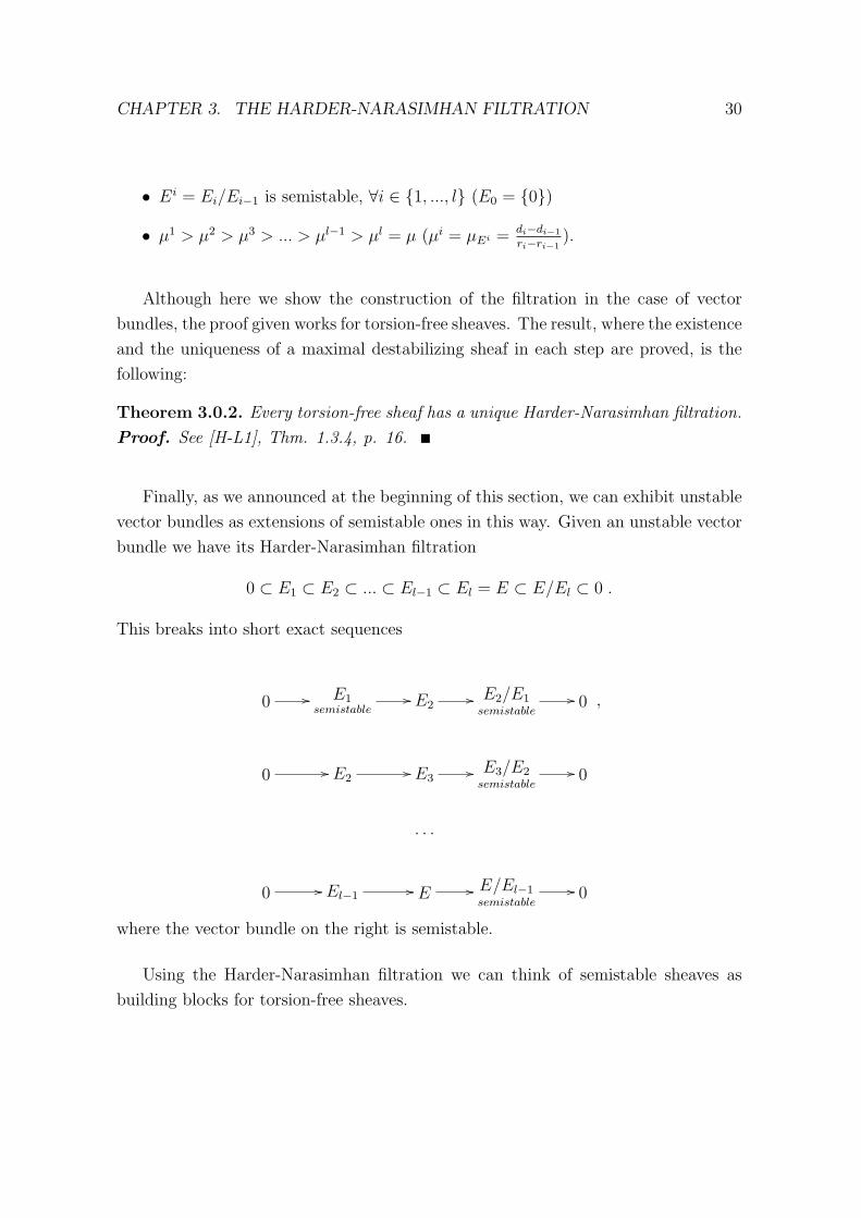
• Ei = Ei/Ei−1 is semistable, ∀i ∈ {1, ..., l} (E0 = {0})

• µ1 > µ2 > µ3 > ... > µl−1 > µl = µ (µi = µEi = di−di−1

ri−ri−1).

Although here we show the construction of the filtration in the case of vector

bundles, the proof given works for torsion-free sheaves. The result, where the existence

and the uniqueness of a maximal destabilizing sheaf in each step are proved, is the

following:

Theorem 3.0.2. Every torsion-free sheaf has a unique Harder-Narasimhan filtration.

Proof. See [H-L1], Thm. 1.3.4, p. 16.

Finally, as we announced at the beginning of this section, we can exhibit unstable

vector bundles as extensions of semistable ones in this way. Given an unstable vector

bundle we have its Harder-Narasimhan filtration

0 ⊂ E1 ⊂ E2 ⊂ ... ⊂ El−1 ⊂ El = E ⊂ E/El ⊂ 0 .

This breaks into short exact sequences

0 // E1semistable

// E2// E2/E1semistable

// 0

0 // E2// E3

// E3/E2semistable

// 0

. . .

0 // El−1// E // E/El−1

semistable// 0

,

where the vector bundle on the right is semistable.

Using the Harder-Narasimhan filtration we can think of semistable sheaves as

building blocks for torsion-free sheaves.


We will show that we can give an easy expression for the Harder-Narasimhan

filtration in the case X = P1C.

Example 3.0.3. Suppose that the curve X is isomorphic to P1C. We know, by an

important theorem of Grothendieck, (see [H-L1], Thm. 1.3.1, p. 14) that a vector

bundle E over P1C splits in line bundles

E = OP1C(a1)⊕OP1

C(a1)⊕...⊕OP1

C(a1)⊕OP1

C(a2)⊕...⊕OP1

C(a2)⊕OP1

C(a3)⊕...⊕OP1

C(as)

with a1 > a2 > ... > as, and we call bi the number of times each line bundle

OP1C(ai) appears. Thus the slope is the average of ai :

µ =degE

rk E=a1b1 + ...+ asbsb1 + ...+ bs

It is clear that

E1 = OP1C(a1)⊕OP1

C(a1)⊕ ...⊕OP1

C(a1)

with

µ1 =a1 +

b1︷︸︸︷· · · +a1

b1= a1 > µ

and

F = E/E1 = OP1C(a2)⊕ ...⊕OP1

C(a2)⊕OP1

C(a3)⊕ ...⊕OP1

C(ar) .

Then also

E2 = OP1C(a2)⊕ ...⊕OP1

C(a2)

which lifts to

E2 = OP1C(a1)⊕OP1

C(a1)⊕ ...⊕OP1

C(a1)⊕OP1

C(a2)⊕ ...⊕OP1

C(a2) .

It is clear that each Ei is semistable and µ1 > µ2 > µ3 > ... > µs−1 > µs = µ.

Chapter 4

The Kempf filtration

We said in Remark 2.4.6 that Geometric Invariant Theory measured, through one-

parameter subgroups, if zero was in the closure of the orbit of a given point or not,

that is, if the point was unstable or not. Understanding one-parameter subgroups as

paths which give a way of approaching a limit point, we can think that there are 1-PS

better than others in the sense that they go to the limit point faster than others.

With this idea, we can say that the Harder-Narasimhan filtration of an unstable

vector bundle represents, in some way, the best one-parameter subgroup. This means

the following: we know that, if E is unstable, there is any 1-PS that destabilizes E,

and the Harder-Narasimhan filtration is the best way to destabilize E, so maybe it

has to correspond to the best one-parameter subgroup, with this point of view.

George R. Kempf, in [Ke], explores this idea generalizing the main results of

Mumford in GIT from an algebraic closed field to a perfect field. He find an ”spe-

cial almost unique” one-parameter subgroup with the best properties, to move most

rapidly toward the origin.

Suppose that E is a GIT-unstable point. Then, there exists a 1-PS λ such that

µ(λ,E) > 0, its minimum relevant exponent. The article of Kempf says that, if

there exists a 1-PS with these conditions, the functionµ(λ,E)

‖λ‖has maximum value

32

CHAPTER 4. THE KEMPF FILTRATION 33

(as a function of λ) and the 1-PS that achieves this maximum is unique, where

‖λ‖ =√∑

i

λ2i is the norm of the 1-PS and µ(λ,E) the minimum relevant exponent.

We will call this 1-PS, the Kempf one-parameter subgroup. It will be the fastest

1-PS which destabilizes our vector bundle E and we will prove that it corresponds to

the Harder-Narasimhan filtration, hence both ideas are really the same.

4.1 Convex cones

Here we are going to describe a pure linear geometry technique which will be very

useful in the developing of the results.

Endow Rt with an inner product (·, ·) defined by a matrix b1

. . .

bt

where bi are positive integers. Let

C ={x ∈ Rt : x1 < x2 < · · · < xt

}Let v = (v1, · · · , vt) ∈ Rt. Define

µv(λ) =(λ, v)

‖λ‖(4.1)

We want to find a vector λ ∈ C which maximizes this function (assuming that there

exists λ ∈ C with µv(λ) > 0).

Let wi = −bivi, w0 = 0, wi = w1 + · · · + wi, b0 = 0, and bi = b1 + · · · + bi.

We draw a graph joining the points with coordinates (bi, wi). Note that this graph

has t segments, each segment has slope −vi and width bi. This is the graph drawn

with a continuous line in the figure. Now draw the convex envelope of this graph

(discontinuous line in the figure), whose coordinates we denote by (bi, wi), and let

λi = −wi/bi. In other words, the quantities −λi are the slopes of the convex envelope

graph. Note that the vector λ = (λ1, · · · , λt) belongs to C by construction.


Remark 4.1.1. If wi > wi, then λi+1 = λi.

bi

wi,w

i

◦��

◦

◦

◦��

��

◦◦@@@@@@◦◦BBBBBBBBB◦◦��

��◦��◦��@@@◦�

��

◦CCCCCC◦��

(b1, w1)

(b1, w1)(b2, w2)

(b2, w2)

(b3, w3 = w3)(b4, w4)

(b4, w4)

(b5, w5 = w5)

Figure 4.1: Graph

Theorem 4.1.2. The vector λ defined in this way gives a maximum for the function

µv.

Before proving the theorem we need some lemmas.

Lemma 4.1.3. Let λ be the point in C which is closest to v. Then λ achieves the

maximum of µv.

Proof. For any α ∈ R>0, the vector αλ is also in C, so in particular λ is the closest

point in the line αλ to v. This point is the orthogonal projection of v into the line

αλ, and the distance is

||v|| sin β(v, λ) (4.2)

where β(v, λ) is the angle between v and λ. But a vector λ ∈ C minimizes (4.2) if

and only if it maximizes

||v|| cos β(v, λ) =(v, λ)

‖λ‖


so the lemma is proved.

We say that an affine hyperplane in Rt separates a point v from C if v is on one side

of the hyperplane and all the points of C are on the other side or on the hyperplane.

Lemma 4.1.4. A point λ ∈ C gives minimum distance to v if and only if the hyper-

plane λ+ (v − λ)⊥ separates v from C.

Proof. ⇒) Assume that there is a point w ∈ C on the same side of the hyperplane

as v. The segment going from λ to w is in C (by convexity), but there are points in

this segment (near λ), which are closer to v than λ.

⇐) Let λ be a point in C such that λ+ (v−λ)⊥ separates v from C. Let w ∈ C be

another point. Let w′ be the intersection of the hyperplane and the segment which

goes from w to v. Since the hyperplane separates C from v, either w′ = w or w′ is in

the interior of the segment. Therefore

d(w, v) ≥ d(w′, v) ≥ d(λ, v) ,

where the last inequality follows from the fact that λ is the orthogonal projection of

v to the hyperplane.

Proof of the theorem. Let λ be the vector in the hypothesis of the theorem.

Using lemmas 4.1.3 and 4.1.4, it is enough to check that the hyperplane λ+ (v− λ)⊥

separates v from C.

Let λ+ ε ∈ C. The condition that λ+ ε belongs to C means that

εi − εi+1 ≤ λi+1 − λi (4.3)

The hyperplane separates v from C if and only if (v−λ, ε) ≤ 0 for all such ε. Therefore

we calculate (using the convention w0 = 0, w0 = 0 and εt+1 = 0)

(v − λ, ε) =t∑i=1

bi(vi − λi)εi =t∑i=1

(−wi + wi)εi =

=t∑i=1

((wi − wi−1)− (wi − wi−1)

)εi =

t∑i=1

(wi − wi)(εi − εi+1)


If wi = wi, then the corresponding summand is zero. On the other hand, if wi > wi,

then λi+1 = λi (Remark 4.1.1), and (4.3) implies εi − εi+1 ≤ 0. In any case, the

summands are always non-positive, and hence (v − λ, ε) ≤ 0.

4.2 The m-Kempf filtration of an unstable bundle

Let E be a vector bundle of rank r and degree d over an algebraic curve X, and

suppose that E is unstable.

Consider the following positive rational number

C = max{(dr− µmax(E))r(r − 1) + gr(r − 1) + 1 , 1},

which we remark that is strictly greater than

(d

r− µmax(E))r(r − 1) + gr(r − 1) ,

where µmax(E) is the maximum slope of the semistable factors of the Harder-Narashiman

filtration of E. Recall that, for any proper subbundle E ′ ⊆ E, it is µmax(E ′) ≤µmax(E).

Any vector subbundle E ′ ⊆ E, of rank r′ and degree d′, such that µ(E ′) < dr−C,

satisfies, for any natural number m, an estimate due to Le Poitier and Simpson (see

[G-S1], [Sch] or [Si]):

h0(E ′(m)) ≤ r′(r′ − 1

r′[d

r+ (

d

r− µmax(E)) +m+ 1]+ +

1

r′[d

r− C +m+ 1]+) ,

where [x]+ = max{0, x}. We denote

m0 := max{−dr− (

d

r− µmax(E))− 1 , −d

r+ C − 1} ,

and we choose m ≥ max{m0,mG}, where mG, depending on g, r, d, is the integer

from which the construction of the moduli space of Gieseker is valid. Then we have


the following bound of the space of global sections of E ′(m):

h0(E ′(m)) ≤ r′(r′ − 1

r′(d

r+ (

d

r− µmax(E)) +m+ 1) +

1

r′(d

r− C +m+ 1))

= r′(d

r+m+ 1 +

r′ − 1

r′(d

r− µmax(E))− C

r′)

≤ r′(d

r+m+ 1 + (

d

r− µmax(E))− C

r′),

so that

h0(E ′(m))r − χ(E(m))r′

≤ r′(d

r+m+ 1 + (

d

r− µmax(E))− C

r′)r − (d+ rm+ r(1− g))r′

= r′(d

r− µmax(E))r + r′r − r(1− g)r′ − rC

= r′(d

r− µmax(E))r + grr′ − rC

≤ (d

r− µmax(E))r(r − 1) + gr(r − 1)− C

hence

h0(E ′(m))r − χ(E(m))r′ < 0. (4.4)

We fix m > max{m0,mG}. Let V be a vector space of dimension h0(E(m)).

Fixing an isomorphism between V and H0(E(m)), and using Gieseker’s construction,

we obtain a point in our orbit space, which is GIT-unstable with respect to the natural

action of SL(V ).

Given a filtration V1 ⊂ · · · ⊂ Vt = V and real numbers λ1 < · · · < λt, we define

the function

µ(V•, λ•) =

∑dimV iλi(r

i dimVdimV i

− r)√∑dimV iλ2

i

where V i = Vi/Vi−1.

Theorem 4.2.1 (Kempf). There is a unique filtration Vi ⊂ V and weights λ1 <

· · · < λt for which Kempf’s function µ(V•, λ•) achieves a maximum.


Remark 4.2.2. Note that this Kempf function is the same as the one given in the

introduction of Chapter 4, where the numerator is the minimum relevant exponent

and the denominator is the norm of the one-parameter subgroup, by associating a

filtration of vector spaces with an 1-PS.

Let V• ⊂ V be the filtration given by Kempf’s theorem. For each i, let Emi ⊂ E

be the subsheaf generated by Vi ⊗OX(−m) under the evaluation map. We call this

filtration, the m-Kempf filtration of E.

Proposition 4.2.3. Every filter Emi in the m-Kempf filtration of E has slope µ(Em

i ) ≥d

r− C.

Proof. Following the notations in Section 4.1 we call vi = −r +dimV · ri

dimV i, bi =

dimV i > 0 (therefore wi = −bi · vi = r · dimV i − dimV · ri). Then the Kempf

function µ(V•, λ•) is the same that the function µv(λ) =(λ, v)

‖λ‖in 4.1.2. See that

wi = w1 + . . .+ wi = r · dimVi − dimV · ri.

If it were µ(Emi ) <

d

r− C for any filter Em

i , then,

wi = r · dimVi − χ(E(m)) · ri ≤ r · h0(Ei(m))− χ(E(m)) · ri < 0,

where the first inequality holds because the dimension of the space of global sections

of Emi is, in general, greater than the dimension of Vi, the vector space of the sections

which generate Emi . The second inequality follows from the bound given in (4.4).

Hence, for that index i, we would have wi < 0. By 4.1.2 this graph must be the

convex envelope as in Figure 4.1, so the slopes have to be decreasing. If for any index

the height of the point in the graph, wi, is negative, it will be wj < 0, for every

j ≥ i, so wt < 0, the last of them. However wt = r dimVt − rt dimV = 0, which is a

contradiction.

On the other hand, it is clear that µ(Emi ) ≤ µmax(E). The important point is that,

although Emi will in general depend on m, its slope is bounded above and below by

numbers which do not depend on m, and furthermore it is a subsheaf of E. Hence, the


set of possible isomorphism classes for Emi is bounded. So we can apply the Vanishing

Theorem of Serre and there is an m1 ≥ max{m0,mG} such that, the sheaves Emi and

Em,i = Emi /E

mi−1 are m1-regular. In particular their higher cohomology groups vanish

and they are generated by global sections. We also assume that m1 is large enough

so that the maximal destabilizing subsheaf of any Em,i is also m1-regular. From now

on, we will assume m ≥ m1.

Proposition 4.2.4. With the previous notations we have that Vi = H0(Emi ), so also

dimVi = h0(Emi ).

Proof. Let Em• ⊆ E the m-Kempf filtration. We know that Vi generates the subsheaf

Emi by definition, so we have the following diagram:

0 ⊂ V1 ⊂ V2 ⊂ · · · ⊂ Vt = V

∩ ∩ ||H0(Em

1 ) ⊂ H0(Em2 ) ⊂ · · · ⊂ H0(Em

t ) = H0(E)

Suppose that there is any index i such that Vi 6= H0(Emi ). Let i be such a subindex

with Vi 6= H0(Emi ) and ∀j > i it is Vj = H0(Em

j ). Then we get the following diagram

Vi ⊂ Vi+1 ⊂ Vi+2 ⊂ ... ⊂ V

∩ || || ||H0(Em

i ) ⊂ H0(Emi+1) H0(Em

i+2) H0(E)

Hence, we have Vi ⊂ H0(Emi ) ⊂ Vi+1 and we consider a new filtration by addition

of the filter H0(Emi ):

0 ⊂ · · · ⊂ Vi ⊂ H0(Emi ) ⊂ Vi+1 ⊂ · · · ⊂ Vt = V

Using again the notations of Section 4.1, let us call

(bi, wi) = (dimVi, dimVi · r − ri · dimV ) ,

the graph of the m-Kempf filtration. Now we consider the graph of the new filtra-

tion, which has two new segments. The old segment linking the points (bi, wi) =


(dimVi, dimVi · r− ri · dimV ) and (bi+1, wi+1) = (dimVi+1, dimVi+1 · r− ri+1 · dimV )

has disappeared.

The new point corresponding to the new filter has coordinates

(h0(Emi ), h0(Em

i ) · r − ri · dimV ) .

Hence, the first of our new segments has slope

(h0(Emi ) · r − ri · dimV )− (dimVi · r − ri · dimV )

h0(Emi )− dimVi

= r

By the other hand, the first one of the slopes is

dimV1 · r − r1 · dimVdimV1

= r − r1 · dimVdimV1

< r .

Then the Kempf function µ(V•, λ•) is the same that the function µv(λ) =(λ, v)

‖λ‖

in 4.1.2, with vi = −r +dimV · ri

dimV i, bi = dimV i > 0 (therefore wi = −bi · vi =

r · dimV i− dimV · ri). Thus, by Theorem 4.1.2, the maximun for the function µv(λ)

is achieved in the convex envelope graph, as in Figure 4.1. But, if a new segment has

slope strictly bigger than another preceding one, the new point has to be in the convex

envelope, so the first filtration could not be the convex envelope. This contradicts

the fact that the first filtration was the maximal filtration.

Therefore Vi = H0(Emi ), for all i.

4.3 Properties of the m-Kempf filtration of E

In the previous section we have seen that, for any m ≥ m1, all the filters Emi of the

m-Kempf filtration of E are m1-regular. Hence, Emi (m1) is generated by the subspace

H0(Emi (m1)) of H0(E(m1)), and the filtration of sheaves

Em1 ⊂ Em

2 ⊂ · · · ⊂ Emt−1 ⊂ Em

t = E


is the filtration associated to the filtration of vector spaces

H0(Em1 (m1)) ⊂ H0(Em

2 (m1)) ⊂ · · · ⊂ H0(Emt−1(m1)) ⊂ H0(Em

t (m1)) = H0(E(m1))

Therefore, for any m ≥ m1, the m-Kempf filtration of E has length t ≤ h0(E(m1)) =:

N1, a bound which does not depend on m.

For each m, the ranks and degrees of the quotients Em,i = Emi /E

mi−1 make a list

of pairs ((r1, d1), (r2, d2), . . .) with length at most N1. Since the ranks and degrees

are bounded (with a bound independent of m), the number of lists which we get is

finite.

Proposition 4.3.1. There is an integer m2 ≥ m1, such that, for m ≥ m2, the

m-Kempf filtration of E has ri > 0 for all i.

Proof. Choose one of the lists of numerical data ((r1, d1), (r2, d2), . . .). Let m ≥ m1

be an integer for which this list is realized. In other words, the m-Kempf filtration

Emi ⊂ E has rk(Em,i) = ri and deg(Em,i) = di. By Kempf’s theorem, we know that

this filtration achieves a maximum of the function

√mµ(V•, λ•) =

∑dimV i

mλim(ri dimV

dimV i− r)√∑

dimV i

mλ2i

among all weighted filtrations (Vi, λi) with λi < λi+1 and Vi ⊂ H0(E(m)). Note that

this function coincides with µv(λ) defined in (4.1) if we set

bi(m) =dimV i

m= ri +

di + ri(1− g)

m

vi(m) = m(ri

dimV

dimV i− r)

=(rid− rdi

) 1

ri + di+ri(1−g)m

Note that we can calculate dimV i in terms of ri and di thanks to Proposition 4.2.4.

Therefore, using Theorem 4.1.2, the graph corresponding to the data bi, vi as in

Figure 4.1 is convex, and λi = vi.

Note that the numbers bi and vi only depend on r, d, ri, di and m. Assume that,

for some i, it is ri = 0. For m′ ≥ m large enough, the graph corresponding to these


numbers is not convex (there is a segment with bi too small, so it tends to a vertical

segment). Therefore, the m′-Kempf filtration of E is not equal to Emi .

We can repeat this argument for each list in which there is some ri = 0, and, since

there is only a finite set of lists, we finally obtain a number m2 ≥ m1 such that, if

m ≥ m2, then the m-Kempf filtration of E has ri > 0 for all i.

Given m > m2, let Emi be the m-Kempf filtration of E. Let m′ > m2 be another

integer. The graph associated to the filtration H0(Emi (m′)) ⊂ H0(E(m′)) using the

data

bi(m′) =dimV i

m′= ri +

di + ri(1− g)

m′

vi(m′) = m′

(ri

dimV

dimV i− r)

=(rid− rdi

) 1

ri + di+ri(1−g)m′

as in Figure 4.1 is called the m′-graph associated to the m-Kempf filtration of E. If

we use the limiting data when m′ tends to ∞

bi(∞) = ri

vi(∞) = d− r

ridi ,

the corresponding graph is called the ∞-graph associated to the m-Kempf filtration

of E.

Proposition 4.3.2. There is an integer m3 ≥ m2, such that, for m ≥ m3, the ∞-

graph and the m′-graph associated to the m-Kempf filtration of E is convex for all

m′ > m.

Proof. Choose one of the lists of numerical data ((r1, d1), (r2, d2), . . .). Let m be an

integer for which this list is realized. In other words, the m-Kempf filtration Emi ⊂ E,

has ri = rk(Em,i) and di = deg(Em,i).

If the ∞-graph of the m-Kempf filtration of E is not convex, then it is also not

convex for any m′ after certain constant. This is because being convex is a closed

condition, and the ∞-graph is the limit of the m′-graphs when m′ tends to infinity.

We repeat this argument for each list, and, since there is only a finite set of lists,

we obtain a constant m3 which satisfies required conditions.


Let m ≥ m3, and consider the m-Kempf filtration of E. Its m-graph is convex, so

the maximum of the function

(√mµv(λ))2 =

(v, λ)2

(λ, λ)

is achieved for λ = v, and the value is

mµv(v)2 = (v, v) =∑(

ri +di + ri(1− g)

m

)((rid− rdi

) 1

ri + di+ri(1−g)m

)2

.

Hence, for each list ((r1, d1), (r2, d2), . . .) of numerical data we have a rational

function on m. We say that f1 ≺ f2 for two rational functions, if the inequality

f1(m) < f2(m) holds for m � 0. From the finite set of functions, let f be the

maximal one with respect to this ordering. Note that this function is unique, because

if f1(m) = f2(m) for infinitely many values of m, then f1 = f2 as functions.

Since we have a finite set of functions, there is a value m4, such that, for m ≥ m4,

the values of f are strictly greater than the values of the other functions.

Proposition 4.3.3. Let m′ and m′′ be integers with m′, m′′ ≥ m4. Then the m′-

Kempf filtration of E is equal to the m′′-Kempf filtration of E.

Proof. By construction, the filtration

H0(Em′

i (m′)) ⊂ H0(E(m′)) (4.5)

is Kempf’s filtration and, by maximality of f , the value of Kempf’s function for this

filtration is f(m′).

Now consider the filtration

H0(Em′′

i (m′)) ⊂ H0(E(m′)) . (4.6)

Since m′′,m′ ≥ m4 (in particular m′ ≥ m1, and then Em′′i is m′-regular) the value

of Kempf’s function for this filtration is also f(m′). Since this value coincides with

the value for Kempf’s filtration of H0(E(m′)), by uniqueness the filtrations (4.5) and

(4.6) coincide. Since m′, m′′ ≥ m1, this implies that the filtrations Em′i and Em′′

i

coincide.

If m ≥ m4, the m-Kempf filtration of E is called the Kempf filtration of E.


4.4 The Kempf filtration is the Harder-Narasimhan

filtration

Finally we see that the Kempf filtration satisfies the properties of the Harder-Narasimhan

filtration given in Chapter 3, so they are the same, by uniqueness of both filtrations.

Let m ≥ m4. Let

0 ⊂ V1 ⊂ · · · ⊂ Vt = V = H0(E(m)) (4.7)

be Kempf’s filtration with weights λ1 < · · · < λt, and let

0 ( E1 ( E2 ( · · · ( Et = E (4.8)

the associated filtration of sheaves, where Ei is the subsheaf generated by Vi ⊗OX(−m).

By the previous work we know that Ei is m-regular for all i, and Vi = H0(Ei(m)).

Using an argument similar to Proposition 4.2.4, we also know that Ei is saturated in

E, i.e., E/Ei is torsion free.

Theorem 4.4.1. The filtration (4.8) coincides with the Harder-Narasimhan filtration

of E.

Proof. We will check that this filtration satisfies the properties of the Harder-

Narasimhan filtration.

Step 1. µ(Ei) > µ(Ei+1)

Kempf’s theorem says that the weighted filtration (4.7) achieves the maximum of

the function ∑ti=1 r

iλi(−dimV i

rir + dimV )√∑t

i=1 riλ2i

If we set bi = ri, vi = −dimV i

rir + dimV , then this is the function µv(λ) in (4.1).

Therefore, λi = vi by Theorem 4.1.2. Since λi < λi+1, we obtain

−dimV i

rir + dimV < −dimV i+1

ri+1r + dimV


dimV i

ri>

dimV i+1

ri+1

Applying Proposition 4.2.4 we get dimV i = H0(Ei(m)) = χ(Ei(m)) (the quotient of

m–regular sheaves is m-regular), and using Riemann-Roch Theorem we obtain

µ(Ei) > µ(Ei+1) .

Step 2. Ei is semistable.

If it is not, let F ⊂ Ei be the maximal destabilizing subsheaf. It is of the form

F = F/Ei−1, with F a subsheaf of Ei. The sheaf F is an extension of m-regular

sheaves, so it is also m-regular, and the sheaf F is the quotient of m-regular sheaves,

so it is m-regular.

Consider the filtration

0 ( E1 ( · · · ( Ei−1 ( F ( Ei ( · · · ( Et = E

and the associated filtration of vector spaces

0 ( V1 ( · · · ( Vi−1 ( H0(F (m)) ( Vi ( · · · ( Vt = V .

By hypothesis, the convex envelope of the graph associated to this filtration is equal

to the graph of the filtration (4.7). This means that the new dot, corresponding to the

new term H0(F (m)), must be on or below the segment joining the dots corresponding

to Vi−1 and Vi. Using the fact that the sheaves involved are m-regular, this implies

µ(F ) ≤ µ(Ei)

but this contradicts the assumption that F is destabilizing.

Appendix A

Simpson construction of the

moduli space

Here we give briefly the construction of the moduli space of vector bundles following

the method of Carlos Simpson (see [Si]).

Let E be vector bundle over an algebraic curve X, of rank r and degree d, and we

suppose E to be slope-semistable. All the vector bundles with these properties are a

bounded family, so we can choose an integer m such that we can apply the Vanishing

Theorem of Serre, in order to have that h1(E(m)) = 0 and E(m) is generated by

global sections. Thus, we can compute their Hilbert Polynomials with the Riemann-

Roch theorem:

χ(E(m)) = h0(E(m)) = deg(E(m)) + r(1− g) = d+ rm+ r(1− g) = N .

In a similar way to the Gieseker method, we have the evaluation morphism

H0(E(m))⊗OX(U)ev� E(m)(U)

s⊗ 1|U 7−→ s|U,

for each open set U in C, and we make a choice of basis to define the surjective

morphism in CN ⊗OX :

46

APPENDIX A. SIMPSON CONSTRUCTION OF THE MODULI SPACE 47

CN ⊗OXα

�� '' ''PPPPPPPPPPPP

H0(E(m))⊗OX ev// // E(m)

.

We take the kernel of each morphism and we obtain the following short exact

sequence:

0 −→ K −→ ONX −→ E(m) −→ 0 ,

where CN ⊗OX = ONX . Now, we twist the sequence with an integer l−m, such that

l � m � 0, to get H1(K(l −m)) = 0 (by the same reasons there exists an l for all

the bounded family). Then,

0 −→ K(l −m)−→ ONX(l −m) −→ E(l) −→ 0 ,

and, taking cohomology,

0 −→ H0(K(l −m))−→H0(ONX (l −m)) −→ H0(E(l)) −→ 0 ,

where the zero in the right corresponds to H1(K(l −m)).

Therefore, pairs {E,α} correspond to quotients H0(ONX (l − m)) � H0(E(l)),

which can be seen as vector subspaces of dimension h0(E(l)) in a vector space of

dimension h0(ONX (l − m)). Thus, we can see our Quot-scheme inside a projective

variety, a Grassmannian:

Quot ⊆ GR(h0(ONX (l −m)), r(l) + (d+ r(1− g))) .

From here, the rest of the process is similar, applying Geometric Invariant Theory

and one-parameter subgroups to our parameter space, to obtain a GIT quotient.

The conclusion is that, the slope-semistable vector bundles we had chosen at the

beginning, are the GIT-semistable points at the end.

Bibliography

[Gi1] D. Gieseker, On the moduli of vector bundles on an algebraic surface, Ann.

Math., 106 (1977), 45–60.

[Gi2] D. Gieseker, Geometric invariant theory and the moduli of bundles, Lecture

Publication Series, IAS/Park City Mathematics Series v.00, (1994)

[Go] T. Gomez Lectures on principal bundles over projective varieties Lectures

given in the Mini-School on Moduli Spaces at the Banach center, Warsaw

(26-30 April 2005)

[G-S1] T. Gomez and I. Sols, Stable tensors and moduli space of orthogonal sheaves,

Preprint 2001, math.AG/0103150.

[G-S2] T. Gomez and I. Sols, Moduli space of principal sheaves over projective vari-

eties, Ann. of Math. (2) 161 no. 2 (2005), 1037–1092.

[Ha] R. Hartshorne, Algebraic Geometry, Grad. Texts in Math. 52, Springer Ver-

lag, 1977.

[H-L1] D. Huybrechts and M. Lehn, The geometry of moduli spaces of sheaves,

Aspects of Mathematics E31, Vieweg, Braunschweig/Wiesbaden 1997.

[H-L2] D. Huybrechts and M. Lehn, Stable pairs on curves and surfaces, J. Alg.

Geom., 4 no. 1 (1995), 67–104.

[H-L3] D. Huybrechts and M. Lehn, Framed modules and their moduli, Intern. J.

Math., 6 no. 2 (1995), 297–324.

48

BIBLIOGRAPHY 49

[Ke] G. Kempf, Instability in invariant theory, Ann. of Math. (2) 108 no. 1

(1978), 299–316.

[Ma] M. Maruyama, Moduli of stable sheaves, I and II. J. Math. Kyoto Univ. 17

(1977), 91–126. 18 (1978), 557–614.

[Mu] D. Mumford, Geometric invariant theory. Ergebnisse der Mathematik und

ihrer Grenzgebiete, Neue Folge, Band 34. Springer-Verlag, Berlin-New York,

1965.

[Ne] P.E. Newstead, Lectures on Introduction to Moduli Problems and Orbit

Spaces, Published for the Tata Institute of Fundamental Research, Bombay.

Springer-Verlag, Berlin (1978).

[Ra] A. Ramanathan, Moduli for principal bundles over algebraic curves: I and

II, Proc. Indian Acad. Sci. (Math. Sci.), 106 (1996), 301–328, and 421–449.

[Sch] A. Schmitt, A universal construction for moduli spaces of decorated vector

bundles over curves, Transformation Groups 161 no. 2 (2004), 167–209.

[Sesh] C.S. Seshadri, Space of unitary vector bundles on a compact Riemann surface.

Ann. of Math. (2) 85 (1967), 303–336.

[Si] C. Simpson, Moduli of representations of the fundamental group of a smooth

projective variety I, Publ. Math. I.H.E.S. 79 (1994), 47–129.

[We] R.O. Wells, Jr., Differential Analysis on Complex Manifolds, Grad. Texts in

Math. 65, Springer Verlag, 1972

Universidad Complutense de Madrid Facultad de Ciencias ... · Universidad Complutense de Madrid...

Documents

Transcript of Universidad Complutense de Madrid Facultad de Ciencias ... · Universidad Complutense de Madrid...