A Laplace’s method for seriesand the semiclassical analysis of epidemiological models

Davide Masoero1, ∗

1Grupo de Fısica Matematica da Universidade de Lisboa

We develop a Laplace’s method to compute the asymptotic expansions of sums of sharply peakedsequences. These series arise as discretizations (Riemann sums) of sharply-peaked integrals, whoseasymptotic behavior can be computed by the standard Laplace’s method. We apply the Laplace’smethod for series to the WKB (i.e. semiclassical) analysis of stochastic models of population biology,with special focus on the SIS model. In particular we show that two different and widely-usedapproaches to the semiclassical limit, i.e. either considering a semiclassical probability distributionor a semiclassical generating function, are equivalent.Keywords: Laplace’s method for series; WKB method; epidemiological models; asymptotic expan-sion; semiclassical analysis; SIS model.

Introduction

In this paper we develop a Laplace’s method to deal with series whose summand is sharply peaked about itsmaximum. More precisely, the main object of the paper is the asymptotic evaluation of the series

I(n, α) = n1−α∞∑k=0

e−nf( knα )g(

k

nα) , α > 0 , n→ +∞ , (1)

with the particular aim of providing a mathematical foundation to the WKB (semiclassical) analysis of epidemiologicalmodels.

The series I(n, α) is actually a Riemann sum, with respect to a homogeneous partition of the positive semi-axisinto subintervals of length 1/nα, of the integral

I(n) = n

∞∫0

e−nf(x)g(x)dx , (2)

and the asymptotic behavior of the latter integral can be computed by the (standard) Laplace’s method provided itapplies, see e.g. [4] [3] [14].

One can expect the series to have the same asymptotic behavior as that of the integral if the partition is fine enough,that is for α big, while under a certain threshold the effects of the discretization cannot be neglected. This is indeedthe case. Depending on the local nature of the global minimum of f , there is an α∗ below which the asymptotics ofthe series and of the integral do not coincide, and the series is oscillatory and even exponentially small with respectto the integral - a pictorial representation of this phenomenon can be found in Figures 1(c) and 1(d) at the end ofSection I.

For example, we will show that if f has a single global minimum point x0 6= 0 such that f ′′(x0) 6= 0 and g(x0) 6= 0then (we refer to Theorem 1 and Corollary 2 for the precise hypotheses and statement)

• if α > 12 ,

I(n, α) ∼ I(n) ∼ e−nf(x0)g(x0)

√2πn

f ′′(x0).

• if α = 12 ,

I(n,1

2) ∼ e−nf(x0)g(x0)

√2πn

f ′′(x0)θ3(−

√nπx0, e

− 2π2

f′′(x0) ) ,

where θ3(z, q) is the third Jacobi theta-function [7]

∗Electronic address: dmasoero@gmail.com

arX

iv:1

403.

5532

v2 [

mat

h-ph

] 2

3 Fe

b 20

15

2

• if α < 12 ,

I(n, α) ∼ n1−αe−nf(x0)g(x0)

(e−

f′′(x0)2 n1−2αt2(nαx0) + e−

f′′(x0)2 n1−2α

(1−t(nαx0)

)2),

where t(x) = min{x− bxc, dxe − x} is the positive triangular wave of height 12 and period 1.

The reader may wonder whether such a seemingly natural object like I(n, α) had not already been studied andwell-understood in the literature. Contrary to our expectations we found few mathematical works devoted to it, themost recent being [18] [16]. Paper [18] deals with the case α = 1

2 (in our notation) and its application to q-polynomialswhile [16] is devoted to the study of a class of hypergeometric functions defined by series that fall in the case α = 1.The thorough discussion of the existing literature contained in [16] shows that the series I(n, α) was never consideredin the general and simple form we do here.

Contrary to the existing works on the subject, our interest does not stem from the asymptotic theory of specialfunctions, but from a branch of applied mathematics in rapid evolution, the semiclassical limit of continuous timeMarkov process, in particular processes related to epidemiological models such as SIS and SIRS models [17]. Thesemiclassical limit of continuous time Markov process originated from the paper [8], where it was noticed that manymodels of population biology (or more in general skip-free continuous time Markov chains) can be solved by a methodsimilar to the WKB method for quantum mechanics in the semiclassical asymptotic regime, see [5], [10], [9], [2], [17]for more recent developments.

The semiclassical regime arises when we consider a population of large size n ∈ N and we assume that either theprobability distribution pk is semiclassical, i.e.

pk ∼ cne−nS( kn )L(k

n) , k ∈ {0, 1, . . . , n}

for some S,L : [0, 1]→ R or the generating function is semiclassical, i.e.

Γ(z) ≡n∑k=0

p(k, n)zk ∼ dnenΣ(z)Λ(z) , z > 0

for some Σ,Λ : [0,∞[→ R. If one of the two hypotheses holds then, accordingly, either S,L or Σ,Λ evolve according toa pair of PDEs of the classical mechanics, a Hamilton-Jacobi equation and a related transport equation. For example,in the SIS model we consider below, these pairs of equations are either equations (41,42) or equations (43,44).

Both approaches have been used with success and it turns out that the generating function plays the role ofthe momentum representation in quantum mechanics [8],[5] [17]. However, it was not at all clear whether the twosemiclassical asymptotic regimes coincide, whether a semiclassical probability distribution implies or not a semiclassicalgenerating function.

We will be able to answer this and other related questions analyzing the generating function by means of theLaplace’s method we will have developed. In fact, if z is real and positive then the generating function is a series ofthe kind I(n, α = 1), namely

Γ(z, n) =

∞∑k=0

e−nf( kn )g(k

n) , f(x) = S(x)− x ln z , g(x) = L(x)χ[0,1] ,

where χ[0,1] is the characteristic function of the unit interval.The Laplace’s method will then allow us to show that if the probability distribution is semiclassical then the

generating function is semiclassical too. It will moreover allow us to compute explicitly Σ and Λ. For example Σ turnsout to be the (restricted) Legendre-Fenchel transform of S, namely Σ(z) = supx∈[0,1]{−S(x) + x ln z}. Among thevarious consequences of these computations - see Section II below - the most important is probably the equivalence,under some reasonable assumptions, of the two approaches to the semiclassical limit of SIS model. This situationshould be compared with the analogous situation in Quantum Mechanics: in Quantum Mechanics the wave functionsin the momentum and position representations are related by the Fourier transform, and in the semiclassical limit thephases of the two wave functions are one the Legendre transform of the other [12].

The paper is divided into two main Sections. In Section I we develop the Laplace’s method for the series I(n, α)while Section II is devoted to the application of Laplace’s method (in the case α = 1) to the semiclassical limit of theSIS model. In Section II we assume that the reader has some knowledge of the classical theory of Hamilton-Jacobiequation.

For the benefit of the reader, we end this Introduction with a summary of our main results about the asymptoticbehavior of I(n, α).

3

Summary of the Asymptotic Behaviors of I(n, α) As it is customary in the Laplace’s method for integrals, andessentially without losing in generality, we suppose that the function f has a single global minimum for x ∈ [0,∞[ andwe identify two different cases, when the minimum point belongs to the open interval ]0,∞[ and when the minimumpoint belongs to the boundary, i.e it is 0.

Global minimum in the open interval Let us assume that I(n, α) converges absolutely for n big enough and thatat the minimum point x0 6= 0 the second derivative does not vanish f ′′(x0) > 0, then

I(n, α) ∼ e−nf(x0)g(x0)

√2πnf ′′(x0) , if α > 1

2√2πnf ′′(x0)θ3(−

√nπx0, e

− 2π2

f′′(x0) )) , if α = 12

n1−α(e−

f′′(x0)2 n1−2αt2(nαx0) + e−

f′′(x0)2 n1−2α

(1−t(nαx0)

)2), if 0 < α < 1

2

(3)

where θ3(z, q) is the third Jacobi theta-function [7] and t(x) = min{x− bxc, dxe − x} .With our assumption on f, g, the asymptotic behavior of the integral (2) can be evaluated via the standard Laplace’s

[14], after which I(n) ∼ e−nf(x0)g(x0)√

2nπf ′′(x0) . Therefore after Theorem 1 we conclude that I(n, α) ∼ I(n) if and

only if α > 12 , while if α < 1

2 then I(n, α) oscillates as a consequence of the coarser discretization.Specializing to the case α = 1, in Theorem 2 we prove that I(n, 1) admits for (locally) smooth f, g an asymptotic

expansion in odd powers of n−12 which coincides term by term with the asymptotic expansion of the integral I(n).

Global minimum attained at the boundary Assuming the global minimum is attained at 0 and f ′(0) > 0, g(0) 6= 0then

I(n, α) ∼ e−nf(0)g(0)

1

f ′(0) , if α > 11

1−e−f′(0) , if α = 1

n1−α , if 0 < α < 1

(4)

Considering that by Watson’s Lemma I(n) ∼ e−nf(0)g(0)f ′(0) ,[14], then in this case the series is asymptotic to the integral,

i.e. I(n, α) ∼ I(n), if and only if α > 1.Specializing to α = 1, we prove in Theorem 4 that I(n) admits for (locally) smooth f, g an asymptotic expansion

in powers of n−1.Acknowledgments We thank P. Miller, A. Raimondo, M. Souza and N. Stollenwerk for fruitful discussions. The work

is supported by the FCT Post Doc Fellowship number SFRH/BPD/75908/2011.

I. LAPLACE’S METHOD FOR SERIES

We begin our discussion of the Laplace’s method for series by selecting a classes of sufficiently tame functions f, gfor which the series I(n, α) converge for all α.

Definition 1. The ordered pair of functions (f, g)

f : [0,∞[→ R ∪ {+∞}g : [0,∞[→ R

is called admissible if the following two conditions hold:

(i) f is bounded from below

(ii) for every α > 0, there exist C,M,m0 > 0 such that such that for all m ≥ m0

|∞∑k=0

e−mF (k/nα)g(k/nα)| ≤ CnMe−mf , f = infx∈[0,∞[

f(x) . (5)

From later on, we will always assume that the functions f, g defining I(n, α) are admissible. In Lemma 1 we give asimple criterion for a pair of functions (f, g) to be admissible. This criterion shows that the conditions on (f, g) arequite mild.

4

Lemma 1. If f : [0,∞[→ R ∪+∞ is bounded from below and it satisfies the inequality

f(x) ≥ c log x for some c > 0 , for x big enough ,

then for any bounded g : [0,∞[→ R, the pair (f, g) is an admissible pair.

Proof. First notice that since g is bounded, the thesis follows if we prove (5) for g the constant function 1.Now we define

F (x) = min{f(x), c log x} .

By construction f(x) ≥ F (x) and inf f = inf F , therefore the Lemma is proved if we show that the bound (5) holdsfor the pair (F, 1).

Now, let [x,∞[ be an half-infinite interval where F coincides with c log x. We can split the series in two subseriesfor which the bound holds

∞∑k=0

e−mF (k/nα) =

bnαxc∑k=0

e−mF (k/nα) +

∞∑k=bnαxc+1

e−mF (k/nα)

The first sum is finite, it contains bnαxc+ 1 terms; all of them are bounded by e−mF . This subseries is thus bounded

by (nαx+ 2)e−mF .Let us now analyze the second subseries. Fixing m0 to be any natural number bigger than 1/c, we get

∞∑k=bnαxc+1

e−mF (k/nα) ≤ e−(m−m0)F∞∑

k=bnαxc+1

e−m0F (k/nα) ≤ κncαn0e−mF ,

where κ = em0F∑∞k=bxc+1 k

−m0c. The thesis is proven.

The peculiar property of the series I(n, α) is that the sequence e−nf(k/nα)

g(k/nα) is sharply peaked around k ∼ nαx0 ,where x0 is the global minimum point of the function f . As a consequence, even though the series depends on everyterm of the sequence, its asymptotic behavior for n large, and actually the full asymptotic expansion of the series,depends only on the Taylor expansion of f and g at x0. This is the important principle of locality or localizationwhich holds also for the integrals that can be evaluated via the Laplace’s method [4], [3], [14].

Following this principle, the main strategy of our proofs is the comparison of the series I(n, α) with a standard one

whose summands model the local behavior of e−nf(k/nα)

g(k/nα) around the global minimum point. In particular, ifthe global minimum is attained at the boundary of the interval then, generically, the local model of f is the linearfunction f(x) = γx for some γ > 0, while if the global minimum point is x0 6= 0 then the local model of f is genericallythe quadratic function f(x) = γ(x− x0)2, γ > 0.

In the first case, the standard series is simply the exponential sum

E(n, α, γ) = n1−α∑k≥0

e−γn1−αk =

n1−α

1− e−γn1−α , α, γ > 0 (6)

the standard series is the Gaussian sum [19]

Q(n, α, γ, x0) = n1−α∑k∈Z

e−n1−2αγ(k−nαx0)2 , α, γ, x0 > 0 . (7)

In fact, we show that the series we consider can be reduced, up to an exponentially small relative error, to (6,7) foran appropriate choice of the parameters. We begin therefore the Section by computing the asymptotic behaviors ofthe Gaussian series for all values of α (exponential sums being trivial). Notice that all these Gaussian series can bewritten in terms of well-known Jacobi Θ functions [7, 15], namely

Q(n, α, γ, x0) =

√nπ

γx0ϑ3

(−nαπ, e−

n2α−1π2

γx0

). (8)

However, the asymptotic regimes we explore here fall in general outside the ones normally considered because, forα 6= 1

2 , both the nome and the variable of the Θ functions depend on n.

5

Lemma 2. The series Q(n, α, γ, x0) (7) has the following asymptotic behavior depending on α > 0:If α > 1

2 then

Q(n, α, γ, x0) =

√πn

γ(1 +O(e−

2πγ n−1+2α

)) . (9)

If α = 12 , then the Gaussian sum is a Jacobi theta function of fixed nome q = e−

π2

γ

Q(n,1

2, γ, x0) =

√πn

γx0θ3(−

√nπx0, e

−π2

γ ) . (10)

Notice that it is a strictly positive periodic function of (√nπx0 − b

√nπx0c).

If α < 12 ,

Q(n, α, γ, x0) = n1−α(P (n, α, γ, x0) +O(e−γn

1−2α

))

(11)

P (n, α, γ, x0) = e−γn1−2αt2(nαx0) + e−γn

1−2α(

1−t(nαx0))2, (12)

where t(x) is the positive triangular wave of height 12 and period 1, namely

t(x) = min{x− bxc} . (13)

Proof. We split the proof into to three cases, corresponding to 1− 2α negative, zero, or positive. The three must bedealt with using different techniques.

In the case 1−2α < 0, the summand does not decrease fast uniformly on n. We transform the series into a tractableone by means of the Poisson summation formula. In this special case, the Poisson summation formula is equivalentto the following renowned (although slightly disguised) identity [15]∑

k∈Ze−n

1−2αγ(k−nαx0)2 = nα−1

√πn

γ

∑q∈2πZ

e−n−1+2α

2γ q(q+2ix0γnα )

The term q = 0 is equal to nα−1√

πnγ . The total contribution of terms q 6= 0 is easily bounded as

|∑

q∈2πZ,q 6=0

e−n−1+2α

2γ q(q+2ix0γnα )| ≤ 2

∑q∈N\{0}

e−2πn−1+2α

γ q = O(e−n−1+2α2π

γ ) .

In the first inequality stems from the fact that q2 ≥ q for q ≥ 1.The case α = 1

2 follows simply from the equation (8).We finally analyze the case 1 − 2α > 0. The maximum of the summand is achieved when nαx0 is closest to 0,

and the corresponding term contributes as e−n1−2αt2(nαx0). The second highest contribution is e−n

1−2α(

1−t(nαx0))2

. Ift(nαx0) ≈ 1

2 then this second contribution cannot be neglected. However, all other contributions are easily bounded,as ∑

k∈Ze−n

1−2αγ(k−nαx0)2 − e−n1−2αγt2(nαx0) − e−n

1−2αγ(

1−t(nαx0))2≤ 2

∑k≥1

e−γn1−2αk = O(e−γn

1−2α

) .

Having collected the asymptotic behavior of the standard series we need, we can now state and prove our Theoremson the Laplace’s method for series I(n, α) (1) for admissible pairs of functions (f, g).

We start by considering the case of f having a global minimum point belonging to the open interval ]0,∞[. InTheorem 1, we compute the leading asymptotic behavior of I(n, α) for a general α. In Theorem 2, we specialize tothe case α = 1 and compute the full asymptotic expansion of I(n, 1), by showing that it coincides at all orders withthe well-known asymptotic expansion of the integral I(n). We prove the latter Theorem by comparing the series andthe integral by means of Euler-McLaurin formula.

6

Theorem 1. For α > 0 consider the series

I(n, α) = n1−α∞∑k=0

e−nf( knα )g(

k

nα)

where (f, g) is an admissible pair of functions. Assume furthermore that

(i) f has a single global minimum point x0 6= 0, f is three-times differentiable in a neighborhood of x0 and f ′′(x0) > 0

(ii) ∃ε > 0 such that

inf|x−x0|>ε

f(x) > f(x0)

(iii) g is differentiable in a neighborhood of x0

Then the following asymptotic formula holds:

• Case α > 12 . For all β s.t. 0 < β < 1

2 ,

I(n, α) =

√2πn

f ′′(x0)e−nf(x0)

(g(x0) +O(n−β)

). (14)

• Case α = 12 . For all β s.t. 0 < β < 1

2 ,

I(n,1

2) = e−nf(x0)

√2πn

f ′′(x0)θ3

(−√nπx0, e

− 2π2

f′′(x0)

)(g(x0) +O(n−β)

). (15)

where θ3 is the third Jacobi Theta function.

• Case 13 < α < 1

2 . For all β s.t. 0 < β < α,

I(n, α) = n1−αe−nf(x0)P

(n, α,

f ′′(x0)

2, x0

)(g(x0) +O(n1−2α−β)

), (16)

where P (n, α, γ, x0) is the oscillating sequence defined in equation (12) above.

• Case 0 < α ≤ 13 . A weaker statement holds

limn→∞

enf(x0)nα−1(I(n, α)− P (n, α,

f ′′(x0)

2, x0)

)= 0 . (17)

Proof. If we multiply the series by sign(g(x0))enf(x0) we reduce to the case f(x0) = 0 and g(x0) ≥ 0 which we assumeto hold. The hypothesis that (f, g) are admissible implies that there exist n ≥ 1, C,M > 0 such that |I(n, α)| ≤ CnMfor all n big enough.

The strategy of the proof goes as follows. First I) we show that terms not sufficiently close to the maximum are

exponentially suppressed, then II) we show can be approximated by the Gaussian sum Q(n, α, f′′(x0)

2 , x0) up to thestated error.

I) After hypotheses (i,ii), we can choose a µ, 0 < µ < f ′′(x0) and δ > 0, such that for any δ ≤ δ0 then f(x) ≥ µδ2

for all |x− x0| ≥ δ.Therefore if |k − nαx0| ≥ nαδ then

nf(k

nα) ≥ (n−m0)µδ2 +m0f(

k

nα) ,∀m0 ∈ R .

Let m0 big enough such that estimate (5) holds, then

|∑

| knα−x0|≥δ

e−nf( knα )g(

k

nα)| ≤ e−(n−m0)µδ2

∑k≥0

|e−m0f( knα )g(

k

nα)| ≤ C ′nM

′e−µnδ

2

, (18)

7

for some C ′,M ′ > 0. Here we used estimate (5) to deduce the last inequality.A slightly stronger version of bound (18) holds for the Gaussian series Q(n, α, γ, x0), γ > 0. In fact,

|Q(n, α, γ, x0)− n1−α∑

|k−nαx0|≥nαδ

e−γn1−2α(k−nαx0)2 | ≤ 2

n1−αe−γnδ2

1− e−γn1−2α ≤ C ′ne−γnδ2

. (19)

Inequalities (18,19) tell us that the total contribution of all terms away from nαx0 is exponentially small as n→ +∞if δ is any small enough fixed positive number. This is also the case if we let δ depend on n according to the lawδ = n−β with 0 < β < 1

2 . This latter choice will be convenient later on in the proof.II)We now give a bound for each term in the sum when k is close to nαx0 using a simple Taylor expansion. Here,

to avoid a cumbersome notation, we suppose g(x0) 6= 0. The few modifications needed to consider the case g(x0) = 0are trivial.

Since g is differentiable at x0 and f has three derivatives at x0 then, for every y small enough, there exists a κ > 0such that if |x− x0| ≤ y then

|f(x)− f(x0) + (x− x0)2f ′′(x0)| ≤ κf ′′(x0)(x− x0)2y and |g(x)− g(x0)| ≤ κy .

Therefore if |k − nαx0| ≤ δnα ≤ ynα

e−nf( knα )g(

k

nα) ≤ e−n

1−2α f′′(x0)

2 (1−κδ)(k−nα)2(g(x0) + κδ)

e−nf( knα )g(

k

nα) ≤ e−n

1−2α f′′(x0)

2 (1+κδ)(k−nα)2(g(x0)− κδ)

Let us analyze the upper-bound. Letting δ = n−β β > 0, we have that for any n is big enough then∑|k−nαx0|≤nα−β

e−nf( knα )g(

k

nα) ≤

∑|k−nαx0|≤nα−β

e−n1−2α(k−nαx0)2

f′′(x0)2 (1−κn−β)

(g(x0) + κn−β

)(20)

Using (18,19) we obtain

I(n, α) ≤ Q(n, α,

f ′′(x0)

2

(1− cn−β

), x0

)(g(x0) + cn−β

)+O(nM

′e−µn

1−2β

) for some M ′ > 0 . (21)

Here we have merged the the error terms coming from (18,19) in a single one, considering that 0 < µ ≤ f ′′(x0)/2.Notice that the bound is effective only for any β, 0 < β < 1

2 , a constraint we assume to hold.By the same reasoning, for the lower bound we obtain

I(n, α) ≥ Q(n, α,

f ′′(x0)

2

(1 + κn−β

), x0

)(g(x0)− κn−β

)+O(nM

′e−µn

1−2β

) for some M ′ > 0 . (22)

We now complete our analysis by considering the four cases α > 1/2, α = 1/2, 1/3 < α < 1/2, α ≤ 1/3 separately.In the case α > 1/2, using (9) we have

Q

(n, α,

f ′′(x0)

2

(1± κn−β

), x0

)(g(x0)± κn−β)

)=

√2πn

f ′′(x0)

(g(x0) +O(n−β)

).

The latter estimate together with inequalities (21,22) implies the thesis.Similarly in the case α = 1

2 , using (10) we have

Q

(n, 1/2,

f ′′(x0)

2

(1± κn−β

), x0

)(g(x0)± κn−β

)=

√2πn

f ′′(x0)θ3(−

√nπx0, e

− 2π2

f′′(x0) )(g(x0) +O(n−β)

),

which, together with inequalities (21,22), proves the thesis. The latter inequality stems from the fact that θ3 and itsderivatives are bounded (in fact periodic) function of the first variable, namely

limε→0

supx∈R|∂yθ3(x, y0 + ε)| = sup

x∈[0,1]

|∂yθ3(x, y0 + ε)| <∞ .

8

For α < 12 the Gaussian series Q(n, α, γ, x0) oscillates between n1−α

(1 +O(e−γn

1−2α

))

and exponentially small

values. More precisely, from (11) we have

P

(n, α,

f ′′(x0)

2

(1± κn−β

), x0

)≥ exp{−n1−2α f

′′(x0)

4(1± κn−β)} .

In order to compare I(n, α) with the Gaussian series we needs to check that the error term in inequalities (21,22) arenegligible with respect to it. To this aim we need to assume that β < α.

From the definition of the function P , equation (11), it follows that for any β > 0

P

(n, α,

f ′′(x0)

2

(1± κn−β

), x0

)(g(x0)± κn−β

)=

P

(n, α,

f ′′(x0)

2, x0

)(g(x0) +O(n1−2α−β)

).

If 1/3 < α < 1/2 then we can find β < α such that n1−2α−β → 0. The thesis is then proved.However, if 0 < α ≤ 1/3 then n1−2α−β 9 0 for any β < α. To prove the thesis in this case, it is sufficient to show

that for any c > 0

limn→∞

nα−1(P (n, α,

f ′′(x0)

2± κn−β , x0)− P (n, α,

f ′′(x0)

2, x0)

)= 0 (23)

To this aim we fix an ε, 0 < ε < α and for any sequence n → ∞, we define nl to be the subsequence such thatt2(nαl x0) ≥ n2α−1+ε

l and nm to be the complementary subsequence. We prove that for both subsequences above limitholds.

From (12), it follows directly that for any c ∈ R

nα−1l

(P (n, α,

f ′′(x0)

2± κn−βl , x0)) ≤ 2e−n

εl (f′′(x0)

2 ±κn−βl ) .

Therefore both terms in (23) tend to zero, so their difference.Conversely, for m→∞ and any β > ε we have that

P (nm, α,f ′′(x0)

2 ± κn−βm , x0)

P (nm, α,f ′′(x0)

2 , x0)= 1 +O(nε−βm ) .

Since P (nm, α,f ′′(x0)

2 , x0)) is bounded then (23) holds.

Corollary 1. With the same hypothesis as in Theorem 1. Let f, g be measurable functions for which I(n) convergesabsolutely for n big enough. If α > 1

2 and g(x0) 6= 0 then I(n, α) ∼ I(n) ≡ n∫∞

0e−nf(x)g(x).

Proof. The thesis follows from the standard Laplace’s method for integrals [14], which states that I(n) ∼√2πnf ′′(x0)g(x0).

Corollary 2. Let f, g satisfy all hypotheses of Theorem 1 and, in addition to that, let us assume that g(x0) 6= 0. Then

I(n, α) ∼ e−nf(x0)g(x0)

√

2πnf ′′(x0) , if α > 1

2√2πnf ′′(x0)θ3(−

√nπx0, e

− 2π2

f′′(x0) )) , if α = 12

n1−αP (n, α, f′′(x0)

2 , x0) , if 13 < α < 1

2

.

Proof. The Corollary is a direct consequence of Theorem 1.

In Theorem 2 below we assess the complete asymptotic expansion of I(n, 1) by directly comparing the series I(n, 1)with the integral I(n) by means of Euler-Mc Laurin summation formula. To this aim, we needs some preparatoryresults, Lemma 3 and Proposition 1.

9

Lemma 3. Let f, g be two functions of one variable with k continuous derivatives then

∂k

∂yke−nf(y/n)g(y/n) =

(k∑l=0

n−l(f ′(y/n)){k−2l,0}Qk,l(y/n)

)e−nf(y/n) (24)

where {j, 0} = max{j, 0} and Qk,l(x) ≡ Qk,l(f ′(x), . . . f (k)(x), g(x), . . . g(k)(x)) are differential polynomials.

Proof. We notice that the thesis is equivalent to

∂k

∂yke−nf(y)g(y) =

(k∑l=0

nk−l(f ′(y)){k−2l,0}Qk,l(y)

)e−nf(y)

We prove the latter statement by induction.If k = 1 the Lemma is trivially true. Suppose the Lemma holds for k we show that it holds for k + 1. In fact

∂k+1k

∂yk+1e−nf(y)g(y) =

∂

∂y

∂k

∂yke−nf(y)g(y) =

(k∑l=0

nk−l+1(f ′(y)){k−2l,0}+1Qk,l(y)+

k∑l=0

nk−l(f ′(y)){k−2l,0}−1({k − 2l, 0}f ′′(y)Qk,l(y) + f ′(y)∂yQk,l(y)

))e−nf(y) =(

k+1∑l=0

nk+1−l(f ′(y)){k+1−2l,0}Qk+1,l(y)

)e−nf(y) .

Here

Qk+1,l =(f ′(y)

)(k−2l,0)Qk,l + {k − 2l + 2, 0}f ′′(y)Qk,l−1(y) + f ′(y)∂yQk,l−1(y) ,

where Qk,k+1 = Qk,−1 = 0 and (k − 2l, 0) = 1 if k − 2l < 0, 0 otherwise. Therefore Qk+1,l is a differential polynomial

in the variables f ′, . . . f (k+1), g, . . . , g(k+1) and the thesis is proven.

The last piece of mathematical technology we need to prove Theorem 2 is a natural extension of the Laplace’smethod.

Proposition 1. Let f, g are measurable functions satisfying the same hypotheses of Theorem 1, and in addition tothem,

g(x) = (x− x0)kr(x) (25)

for some k ≥ 0 and some continuous function r(x).Then for any x∗ > x0

n

x∗∫0

e−nf(x)g(x)dx = O(n1−l2 ) .

Proof. See e.g. [6] page 37.

Theorem 2. With the same hypothesis of Theorem 1. Consider the series

I(n) ≡ I(n, 1) =

∞∑k=0

e−nf( kn )g(k

n)

where f, g are measurable functions such that for some m ≥ 0

(i) f has m+ 2 continuous derivatives in a neighborhood of x0.

(ii) g has m+ 1 continuous derivatives in a neighborhood of x0.

10

For any x∗ > x0

enf(x0)(I(n, α)− n

x∗∫0

e−nf(x)g(x)dx)

= o(n−bm2 c+

12 ) (26)

Due to the well-known [14] asymptotic expansion of I(n), formula (26) implies that

I(n) =

√2nπ

f ′′(x0)e−nf(x0)

g(x0) +

bm2 c∑l=1

aln−l + o(n−m)

(27)

where al, l = 1, . . . ,m depends on the first l + 2, l derivatives of f, g at x0.

Proof. If we multiply the series by enf(x0) we reduce to the case f(x0) = 0.In the proof of Theorem 1 we proved that the total contributions of terms where |k − nx0| > nδ for a fixed δ > 0

o(n−K) for all K > 0. The same principle holds for the integral [14] : for any x1, x2 > x0

x1∫0

e−nf(x)g(x)dx =

x2∫0

e−nf(x)g(x)dx+ o(n−K) , ∀K > 0 .

Therefore to prove the thesis it will suffice to show that

nn0∑k=0

e−nf(k/n)g(k/n) =

n0∫0

e−nf(x)g(x)dx+ o(n−bm2 c+

12 ) . (28)

Moreover, without losing generality, we can assume that f, g have m + 2,m + 1 continuous derivative in the wholesegment [0, n0].

To prove the above statement, we use Euler(-McLaurin) summation formula, according to which (see e.g. [1]) forany (integrable) function h with 2p (resp. 2p+ 1) continuous derivatives the following formula holds

N∑k=0

h(k) =

n∫0

h(y)dy +h(N)− h(0)

2−

p∑k=1

B2k

(2k)!(h(2k−1)(N)− h(2k−1)(0)) +R (29)

R = C2p

N∫0

B2p(y)h(2p)(y)dy = C2p+1

N∫0

B2p+1(y)h(2p+1)(y)dy .

Here B2k is the 2k-th Bernoulli number, Bj(y) is the j-th periodic Bernoulli function, which is a j−2 times differentiableperiodic function of period 1 and finally Cj is a universal constant; see [1] for the precise definitions.

We apply the formula to h(y) = e−nf(y/n)g(y/n) and N = nn0 to get

I(n) = n

n0∫0

e−nf(x)g(x)dx+ remainder

where the remainder is made of contribution from the evaluation at the endpoint of the interval -which are discardedbecause exponentially small- and the term R, involving the integral of h(m+1) as by hypothesis h has m+1 continuousderivatives.

In order to show that R = o(n−m−1

2 ), we first make use of Lemma 3 to obtain a first expansion of R in power seriesof n

R = n

n0∫0

Bm+1(xn)e−nf(x)

(m+1∑l=0

n−l(f ′(x)){m+1−2l,0}Qm+1,l(x)

)dx ,

where {j, 0} = max{j, 0}.Since f ′(x0) = 0 (x0 is a minimum for f), then (f ′(x)){m+1−2l,0}Ql,k(f(x), g(x)) = (x− x0){m+1−2l,0}rm+1,l(x) for

some continuous function rl.

11

After Proposition 1, we can conclude that there are C0, . . . , Cm+1 > 0 such that

|R| ≤ n1/2

(m+1∑l=0

Cln−ln−{m+1−2l,0}/2

)= O(n−m/2) = o(n−

m−12 ) .

Corollary 3. If f, g satisfy the hypotheses of Theorem 2 and in addition they are smooth in the neighborhood of theunique global minimum point x0 of f , then I(n) admits an asymptotic expansion in odd (negative) powers of n

12 that

coincides with the asymptotic expansion of I(n).

We turn now our attention to the asymptotic evaluation of I(n, α) when the global minimum point is 0. In Theorem 3we deal with the leading asymptotic behavior of I(n, α) for general α, and in Theorem 4 we compute the full asymptoticexpansion in the case α = 1.

Theorem 3. For α > 0 consider the series

I(n, α) = n1−α∞∑k=0

e−nf( knα )g(

k

nα)

where (f, g) is an admissible pair of functions. Assume furthermore that

(i) f has a single global minimum at x = 0, it is differentiable in a neighborhood of 0 and f ′(0) > 0

(ii) there exists an ε such that

infx>ε

f(x) > f(0)

(iii) g is differentiable in a neighborhood of 0

Then the following asymptotic formula holds:

• Case α > 1. For all β s.t. 0 < β < 1 et β < α− 1,

I(n, α) =e−nf(0)

f ′(0)(g(0) +O(n−β)) . (30)

• Case α = 1. For all β s.t. 0 < β < 1

I(n) =e−nf(0)

1− e−f ′(0)(g(0) +O(n−β)) . (31)

• Case 0 < α < 1. For all β s.t. 0 < β < 1

I(n, α) = nα−1e−nf(0)g(0)(1 +O(n−β)) . (32)

Proof. The proof follows the same strategy as the proof of Theorem 1.If we multiply the series by enf(x0)sign(g(0)) we reduce to the case f(0) = 0, g(0) ≥ 0. Since (f, g) are admissible,

∃n0, C,M > 0 such that for n ≥ n0, I(n, α) ≤ CnM .We notice that only contributions localized at k = 0 do matter asymptotically. Indeed, there exist µ, δ0, C

′,M ′ suchthat for any δ ≤ δ0

|∑k≥nαδ

e−nf( knα )g(

k

nα)| ≤ C ′nM

′e−µnδ . (33)

To prove the latter bound we follow the same steps as in Theorem 1. Namely we notice, after hypotheses (i,ii) on f ,that if δ > 0 is small enough there exists a 0 < µ < f ′(0) such that f(x) ≥ µδ for all x ≥ δ. Therefore for any δsufficiently small

nf(k

nα) ≥ (n−m0)µδ +m0f(

k

nα); .

12

Estimate (33) follows from the latter bound, by choosing m0 big enough so that bound (5) holds.If δ is fixed or δ = n−β with 0 < β < 1, then the total contribution of all terms for k ≥ nαδ is exponentially small.

The same principle holds also for the exponential series E(n, α, γ) (6) which is just a special case of I(n, α) withf(x) = γx, g(x) = 1: we have the slightly stronger bound

|∑k≥nαδ

e−γn1−αk| ≤ CnMe−γnδ for some C,M > 0 . (34)

As in the proof of Theorem 1, we compare, the truncated I(n, α) with the exponential series. Again, to avoid acumbersome notation, we suppose g(0) 6= 0. The few modifications needed to consider the case g(x0) = 0 are trivial.Since f is twice differentiable at 0 and g is differentiable at 0 then then, for every y small enough, there exists a κ > 0such that if x ≤ y then

|f(x)− (x− x0)f ′(0)| ≤ κf ′(0)xy and |g(x)− g(0)| ≤ κy .

Therefore if k ≤ δnα ≤ ynα

e−nf( knα )g(

k

nα) ≤ e−n

1−αf ′(0)(1−κδ)k(g(0) + κδ)

e−nf( knα )g(

k

nα) ≥ e−n

1−αf ′(0)(1+κδ)k(g(0)− κδ)

Let us analyze the upper-bound. Letting δ = n−β β > 0, we have that for any n is big enough∑k≤nα−β

e−nf( knα )g(

k

nα) ≤

∑k≤nα−β

e−n1−α(f ′(0)−κn−β)k(g(x0) + κn−β)) (35)

Using (33,34) we obtain

I(n, α) ≤ E(n, α, f ′(0)− κn−β

) (g(0) + κn−β

)+O(nM

′e−µn

1−β) for some M ′ > 0 . (36)

Here we have merged the error terms from (33,34) into a single one, considering that µ < f ′(0). Notice that the boundis effective only for any β, 0 < β < 1, a constraint we assume to hold.

The same analysis shows that we have the lower bound

I(n, α) ≤ E(n, α, f ′(0) + κn−β

) (g(0)− κn−β

)+ O(nM

′e−µn

1−β) for some M ′ > 0 . (37)

After equation (6) for E(n, α, γ), the following formulas hold

nα−1E(n, α, f ′(0)± κn−β

) (g(0)∓ κn−β

)=

g(0)+O(n−β)

f ′(0) , if α > 1g(0)+O(n−β)

1−e−f′(0) , if α = 1

n1−αg(0)(1 +O(n−β)) , if α < 1

The thesis follows after the latter formula and the estimate (36,37).

Before introducing and proving Theorem 4 about the asymptotic expansion of the series I(n, 1), we introduce herea last estimate we need to prove them.

Lemma 4. Let f, g : [0,∞[→ R be two functions such that, for some m ≥ 0,

• f has m+ 2 continuous right derivatives at x = 0 and f(0) = 0

• g has m+ 1 continuous right derivatives at x = 0

Fix β > 12 . On the set {n ≥ 1, k ≤ n1−β} the following estimate hold∣∣∣∣∣e−nf(k/n)g(k/n)− e−f

′(0)k(g(0) +

m∑l=1

Pl(k)n−l)∣∣∣∣∣ ≤ n−m−1e−f

′(0)kR(k) .

where

Pl(k) = ef′(0)k 1

l!

(∂l

∂(n−1)le−nf(k/n)g(k/n)

)n=∞

.

and R(k) is some polynomial in k.

13

Proof. Notice that −nf(k/n) + f ′(0)k = O(n1−2β). Since β > 12 then we can expand e−nf(k/n)+f ′(0)k, in power

series of (−nf(k/n) + f ′(0)k). The thesis then follows by applying Taylor’s formula to the function F (n; k) =

e−nf(k/n)+f ′(0)kg(k/n).

Theorem 4. Consider the series

I(n) =

∞∑k=0

e−nf( kn )g(k

n)

where f, g satisfy the same hypotheses as in Theorem 3, and in addition to them, there exists an m ≥ 0 such that

(i) f has m+ 2 continuous derivatives in a (right-)neighborhood of 0

(ii) g has m+ 1 continuous derivatives in a (right-)neighborhood of 0

then

I(n, 1) = e−nf(0)

(g(0)

1− e−f ′(0)+

m∑l=1

aln−l + o(n−m)

)(38)

where

al =∑k≥0

e−kf′(0)Pl(k), Pl(k) =

(∂l

∂(n−1)le−n

∑m+1j=2

f(l)(0)j!

kj

nj g(k/n)

)n=∞

. (39)

Proof. As usual, we multiply the series by enf(x0)sign(g(0)) we reduce to the case f(0) = 0, g(0) ≥ 0. Since (f, g) areadmissible, ∃n0, C,M > 0 such that for n ≥ n0 I(n, α) ≤ CnM .

A trivial extension of the estimate (34) implies that if β < 1 then for any polynomial P (k) there exist C ′,M ′ suchthat

|∑

k/n≥n−βe−γkP (k)| ≤ C ′nM

′e−γn

1−β.

The thesis follows from the latter bound, estimate (33) and Lemma (4).

Corollary 4. With the same hypothesis of Theorem 3. Let f, g be measurable functions, α > 1 and g(x0) 6= 0 thenfor any x∗ > 0

I(n, α) ∼ nx∗∫0

e−nf(x)g(x) .

Proof. The standard Watson’s Lemma [14] implies that

n

x∗∫0

e−nf(x)g(x) ∼ e−nf(x0)

f ′(x0)g(x0) .

The thesis follows from the latter result and (30) of Theorem 1.

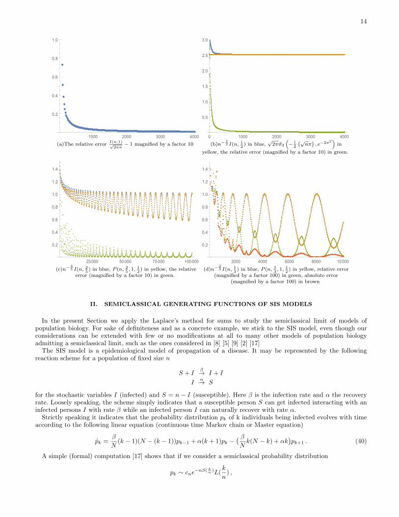
A Numerical Example

We consider the series I(n, α) for functions f(x) = 116 − x

2 + 2x3 − x4 if x ∈ [0, 1], +∞ otherwise, and g(x) = 1.

Functions f, g satisfy the hypotheses of Theorem 1. The global minimum point of f is 12 and f( 1

2 ) = 0, f ′′( 12 ) = 1.

In Theorem 1, we identified 4 different kind of asymptotic behaviors of the series I(n, α) according to whetherα > 1

2 , α = 12 ,

13 < α < 1

2 , 0 < α ≤ 13 .

To show the different behaviors, below we plot I(n, 1), I(n, 12 ), I(n, 2

5 ) and I(n, 13 ) against the dominant term in the

asymptotic expansion, respectively√

2πn,√

2πnϑ3

(− 1

2 (√nπ) , e−2π2

), n

35P (n, 2

5 ,12 ,

12 ) , and n

23P (n, 1

3 ,12 ,

12 ), where

the function P is defined by formula (12).

From Plot 1(d), one can see that sequence of the relative errorsI(n, 13 )

P (n, 13 )− 1 has a peak corresponding to any local

minimum of P (n, 13 ). These peaks prevent this sequence to tend to 0. Conversely the absolute error tends to 0. Both

phenomena were predicted in the Corollary 2 and its proof.

14

1000 2000 3000 4000

0.2

0.4

0.6

0.8

1.0

(a)The relative errorI(n,1)√

2πn− 1 magnified by a factor 10

0 1000 2000 3000 4000

0.5

1.0

1.5

2.0

2.5

3.0

(b)n−12 I(n, 1

2) in blue,

√2πϑ3

(− 1

2

(√nπ

), e−2π2

)in

yellow, the relative error (magnified by a factor 10) in green.

25000 50000 75000 100000

0.2

0.4

0.6

0.8

1.0

1.2

1.4

(c)n−35 I(n, 2

5) in blue, P (n, 2

5, 1, 1

2) in yellow, the relative

error (magnified by a factor 10) in green.

2000 4000 6000 8000 10000

0.2

0.4

0.6

0.8

1.0

1.2

1.4

(d)n−23 I(n, 1

3) in blue, P (n, 1

3, 1, 1

2) in yellow, relative error

(magnified by a factor 100) in green, absolute error(magnified by a factor 100) in brown

II. SEMICLASSICAL GENERATING FUNCTIONS OF SIS MODELS

In the present Section we apply the Laplace’s method for sums to study the semiclassical limit of models ofpopulation biology. For sake of definiteness and as a concrete example, we stick to the SIS model, even though ourconsiderations can be extended with few or no modifications at all to many other models of population biologyadmitting a semiclassical limit, such as the ones considered in [8] [5] [9] [2] [17]

The SIS model is a epidemiological model of propagation of a disease. It may be represented by the followingreaction scheme for a population of fixed size n

S + Iβ→ I + I

Iα→ S

for the stochastic variables I (infected) and S = n − I (susceptible). Here β is the infection rate and α the recoveryrate. Loosely speaking, the scheme simply indicates that a susceptible person S can get infected interacting with aninfected persons I with rate β while an infected person I can naturally recover with rate α.

Strictly speaking it indicates that the probability distribution pk of k individuals being infected evolves with timeaccording to the following linear equation (continuous time Markov chain or Master equation)

pk =β

N(k − 1)(N − (k − 1))pk−1 + α(k + 1)pk −

( βNk(N − k) + αk

)pk+1 . (40)

A simple (formal) computation [17] shows that if we consider a semiclassical probability distribution

pk ∼ cne−nS( kn )L(k

n) ,

15

then, discarding higher order contribution O(1/n), S and L evolves according to a pair of PDEs of classical mechanics

St +H(x, Sx) = 0 , H(x, q) = −αx(eq − 1) + βx(x− 1)(e−q − 1) (41)

Lt + ∂qH(x, q)|q=SxLx +(1

2∂2qH(x, q)|q=SxSxx + ∂q∂xH(x, q)|q=Sx

)L = 0 (42)

Equation (41) is the Hamilton-Jacobi equation, equation (42) is a transport equation. They both can be solved viathe method of characteristics [12].

A similar (formal) computations [17] shows that also if the generating function is semi-classical

Γ(z) =

n∑k=0

pkzk ∼ dnenΣ(z)Λ(z)

then its evolution is described up to O(1/n) correction by a (different) pair of Hamilton-Jacobi and transport equations

Σt + Θ(z,Σz) = 0 , Θ(z, q) = −(βz − α)(z − 1)q + βz2(z − 1)q2 (43)

Λt + ∂qΘ(z, q)|q=ΣzΛz +(1

2∂2qΘ(z, q)|q=ΣzΣzz + β(−z + z2)Σz

)Λ = 0 (44)

Both approaches to the semiclassical limit of systems of population biology have been used with success withinthe physical literature, see e.g. [8] [5] [9] [17]; depending on the specific problem they offer different advantages. Thegenerating function is often useful as it seems to play the role of the momentum-representation in quantum mechanics[8]. Currently we are studying the long-time behavior of the semiclassical approximation and the generating functionturns out to be extremely useful to overcome the singularities that the general solution to Hamilton-Jacobi develops[13].

However, there was so far no proof that the two approaches are equivalent, in the sense that they apply to thesame asymptotic regime, or in cruder words there was no proof that a semiclassical probability distribution impliesa semiclassical generating function. It was even unknown whether the semiclassical equations, which are nonlinear,preserve the total probability.

After our Theorems on the Laplace’s method for sums, we can prove that the two approaches are equivalent andthat the total probability is conserved. We can thus furnish a minimal kynematical foundation for the semiclassicaldynamics of the SIS model, by a method that is valid for all other equation of population biology (Markov processes)that allows a similar semiclassical limit.

Our main results are as follows

• Theorem 5. First we show that if pk is semiclassical then also Γ(z) is semiclassical and we compute explicitly Σand Λ. Σ turns out to be the (restricted) Legendre-Fenchel transform of S.

• Theorem 6. Then we show that the Σ,Λ we obtained satisfy the semiclassical PDEs (43,44) provided S,L satisfythe semiclassical PDEs (41,42).

• Theorem 7. Eventually we show, using the semiclassical dynamics of the generating function, that the totalprobability is asymptotically conserved. We prove that

n∑k=0

e−nS( kn ,t)L(k

n, t) ∼

n∑k=0

e−nS( kn ,0)L(k

n, 0)

if S,L satisfy (41,42).

We warn the reader that the proofs of Theorem 6 and Theorem 7 require some knowledge of the method of charac-teristics for the solution of Hamilton-Jacobi equations.

Theorem 5. Consider the generating function of a semiclassical probability distribution

Γ(z, n) =

n∑k=0

e−S( kn )L(k

n) ,

where

1. S : [0, 1]→ R ∪ {+∞} is a continuous function, three times differentiable on ]0, 1[, and with a single minimumat x0 ∈]0, 1[ and such that S′′(x) 6= 0,∀x ∈]0, 1[.

16

2. L : [0, 1]→ R is a never vanishing differentiable function.

Then for any z > 0

Σ(z) ≡ limn→∞

ln Γ(z, n)

n= supx∈[0,1]

{−S(x) + x ln z} . (45)

Moreover, for any z, eS′(0) < z < eS

′(1) let x(z) be the unique solution of f ′(x) = lnz. Then

Γ(z) ∼ enΣ(z)

1

1−exp(−S′(1)+log z

)L(1) , if z > eS′(1)√

πn2S′′(1)L(1) , if z = eS

′(1)√2πn

S′′(x(z))L(x(z)) , eS′(0) < z < eS

′(1)√πn

2S′′(0)L(0) , if z = eS′(0)

1

1−exp(−S′(0)+log z

)L(0) , if z < eS′(0)

(46)

In particular for z, eS′(0) < z < eS

′(1) the following formula holds

Γ(z) ∼√

2πnenΣ(z)Λ(z) with Λ(z) =L(x(z))√S′′(x(z))

(47)

Proof. For z > 0 we can write Γ(z) =∑∞k e−nf( kn )g( kn ) where f(x) = S(x)−x ln z and g(x) = Λ(x)χ[0,1]. Here χ[0, 1]

is the characteristic function of the unit interval, namely χ[0, 1](x) = 1 if x ∈ [0, 1], 0 otherwise. The thesis followsdirectly from Theorems 2 and 4.

The only two cases not treated explicitly in the above mentioned Theorems are when z = eS′(0) or z = eS

′(1). Herethe maximum of the summand is achieved at the boundary, where the first derivative (but not the second) vanishes.It is easily seen that this case is analogous to the one treated in Theorem 2, the only difference being a 1

2 factor.

Corollary 5. With the same hypotheses of Theorem 5.

Γ(1, n) =

n∑k=0

pk ∼

√2πn

S′′(x0)e−nS(x0)L(x0) (48)

where x0 is the unique global minimum point of S.

Remark. Formula 45 shows that Σ is the (restricted) Legendre-Fenchel transform of S evaluated at ln z [11].

We can now prove now that Σ,Λ defined as in (45, 47) satisfy the semiclassical PDEs (43,44) provided S,L satisfythe semiclassical PDEs (41,42).

Theorem 6. Let S(x, t), L(x, t), t ∈ [0, T [ be solutions of equations (41,42) satisfying the hypotheses of Theorem 5

for all t’s , and let Γ be the generating functions, Γ(z, t) ≡∑k e−nS( kn ,t)L( kn , t).

Then

1. Σ(z, t) = limn→∞log Γ(z,t)

n exists and satisfies equations (43) for any z > 0.

2. For any z, eSx(0,t) < z < eSx(1,t),

Γ(z, t) ∼√

2πnenΣ(z,t)Λ(z, t)

where Λ(z, t) satisfies (44).

Proof. By Theorem 5, Σ is the (restricted) Legendre-Fenchel transform of S evaluated at ln z. Therefore [11] letting

Σ(y, t) = Σ(ey, t) and y(x, t) = Sx(x, t), the following identity holds

S(x, t) + Σ(y(x, t), t) = xy(x, t) .

Differentiating by t, we get

St + Σt = yt(x− Σy(y(x, t), t)) .

17

Since x = Σy(y(x, t), t) (x, y are the conjugate variables of Legendre transform) then

Σt(y, t)−H(Σy, y) = 0 or equivalently Σt(z, t)−H(zΣz, ln z) = 0 .

A simple computation shows that −H(zq, ln z) = Θ(z, q), for any z, q.A similar, but more involved, computation shows that Λ satisfies the transport equation. Details can be found, for

example, in the proof of Theorem 5.3 in [12]. We omit to reproduce here those computations since they require muchmore machinery from Hamilton-Jacobi theory than the one appropriate for the present paper.

Using the semiclassical equations for Γ(z), we can show that the semiclassical dynamics conserves the total proba-bility.

Theorem 7. Let S(x, t), L(x, t), t ∈ [0, T [ be solutions of equations (41,42) satisfying the hypotheses of Theorem 5for all t’s. Then

n∑k=0

e−nS( kn ,t)L(k

n, t) ∼

n∑k=0

e−nS( kn ,0)L(k

n, 0) , ∀t ∈ [0, T [ . (49)

Proof. After Theorem 5, we have∑nk=0 e

−nS( kn ,t)L( kn , t) ∼ enΣ(1,t)Λ(1, t). To prove the thesis it is sufficient to showthat Σ(1, t) and Λ(1, t) are constant in time. We do that by means of the method of characteristics:

On the solution of the system of ODEs

z = ∂qΘ(z, q), q = −∂zΘ(z, q), q(0) = Σz(z, 0)

then

Σ(z(t)) = Σ(z(0)) +

t∫0

∂qΘ(z(s), q(s))q(s)ds

Λ(z(s)) = Λ(z(0))−t∫

0

(1

2∂2qΘ(z(s), q(s))Σzz(z(s)) + β(−z(s) + z2(s))Σz(z(s))

)ds .

Since z = 0 if z = 0 then the characteristic starting at z = 0 will stay in z = 0 for all t. Moreover, the integrals definingS,L vanish for all t as the integrands vanish identically at z = 0. Therefore Σ(1, t) = Σ(1, 0),Λ(1, t) = Λ(1, 0).

Remark. We can actually relax the hypotheses of Theorem 7. Indeed it holds, with a slightly more complex proof, ifwe just requires that S′′(x, 0) and L(x, 0) do not vanish in a neighborhood of the global minimum of S(x, 0).

An apparent paradox concerning the meta-stable state of SIS model

It has been noticed in many models of population biology, see e.g. [2, 10, 17], that the in the semiclassical regimethe meta-stable states of the model correspond to non-trivial stationary solutions of the Hamilton-Jacobi equation.

Assuming βα > 0, the SIS model admits a quasi-stationary or meta-stable state p∗, corresponding to an exponentially

small eigenvalue of the transition matrix of the Markov chain (40), see [17].In the semiclassical regime and considering the probability distribution picture, the meta-stable state corresponds

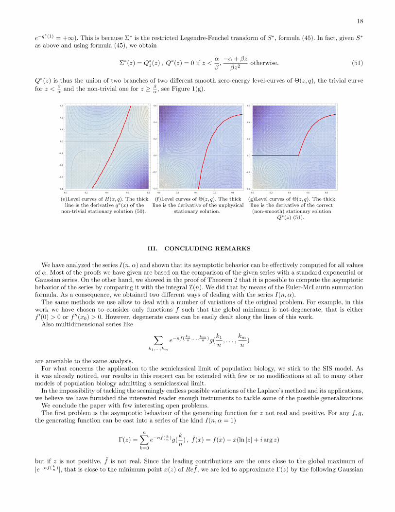
to a non-trivial stationary solution S∗ of the Hamilton-Jacobi equation (41). This in turn corresponds to a zero-energylevel-curve of the Hamiltonian as clearly S∗t = 0 if and only if H(x, S∗x(x)) = 0. Explicitly [17] (see Figure 1(e))

S∗(x) = q∗x(x) , q∗(x) = logβ(1− x)

α(50)

Surprisingly, in the generating function picture such meta-stable state seems to be missing. In fact, since for anyprobability distribution pk ≥ 0,∀k then meta-stable state should correspond to zero-energy level-curves of the Hamil-tonian Θ(z,Q∗(z)) such that Q∗(z) ≥ 0. However, the only non-trivial smooth energy-level curve of the Hamiltonian is−α+βzβz2 that tends to −∞ as z → 0+, see Figure 1(f). This seems to contradict Theorem 6, after which any stationary

solution to (41) corresponds to a stationary solution of (43).The solution of this apparent paradox comes from Theorem 5. After this Theorem, we know that Σ∗ is not smooth

even if S∗ is smooth. Indeed the second derivative of Σ∗ is discontinuous at z = eq∗(0), z = e−q

∗(1) (in this case

18

e−q∗(1) = +∞). This is because Σ∗ is the restricted Legendre-Fenchel transform of S∗, formula (45). In fact, given S∗

as above and using formula (45), we obtain

Σ∗(z) = Q∗z(z) , Q∗(z) = 0 if z <

α

β,−α+ βz

βz2otherwise. (51)

Q∗(z) is thus the union of two branches of two different smooth zero-energy level-curves of Θ(z, q), the trivial curve

for z < βα and the non-trivial one for z ≥ β

α , see Figure 1(g).

0.0 0.2 0.4 0.6 0.8

-0.4

-0.3

-0.2

-0.1

0.0

0.1

0.2

0.3

(e)Level curves of H(x, q). The thickline is the derivative q∗(x) of the

non-trivial stationary solution (50).

0.0 0.2 0.4 0.6 0.8

-0.4

-0.2

0.0

0.2

0.4

0.6

(f)Level curves of Θ(z, q). The thickline is the derivative of the unphysical

stationary solution.

0.0 0.2 0.4 0.6 0.8

-0.4

-0.2

0.0

0.2

0.4

0.6

(g)Level curves of Θ(z, q). The thickline is the derivative of the correct(non-smooth) stationary solution

Q∗(z) (51).

III. CONCLUDING REMARKS

We have analyzed the series I(n, α) and shown that its asymptotic behavior can be effectively computed for all valuesof α. Most of the proofs we have given are based on the comparison of the given series with a standard exponential orGaussian series. On the other hand, we showed in the proof of Theorem 2 that it is possible to compute the asymptoticbehavior of the series by comparing it with the integral I(n). We did that by means of the Euler-McLaurin summationformula. As a consequence, we obtained two different ways of dealing with the series I(n, α).

The same methods we use allow to deal with a number of variations of the original problem. For example, in thiswork we have chosen to consider only functions f such that the global minimum is not-degenerate, that is eitherf ′(0) > 0 or f ′′(x0) > 0. However, degenerate cases can be easily dealt along the lines of this work.

Also multidimensional series like ∑k1,...,km

e−nf(k1n ,...,

kmn )g(

k1

n, . . . ,

kmn

)

are amenable to the same analysis.For what concerns the application to the semiclassical limit of population biology, we stick to the SIS model. As

it was already noticed, our results in this respect can be extended with few or no modifications at all to many othermodels of population biology admitting a semiclassical limit.

In the impossibility of tackling the seemingly endless possible variations of the Laplace’s method and its applications,we believe we have furnished the interested reader enough instruments to tackle some of the possible generalizations

We conclude the paper with few interesting open problems.The first problem is the asymptotic behaviour of the generating function for z not real and positive. For any f, g,

the generating function can be cast into a series of the kind I(n, α = 1)

Γ(z) =

n∑k=0

e−nf( kn )g(k

n) , f(x) = f(x)− x(ln |z|+ i arg z)

but if z is not positive, f is not real. Since the leading contributions are the ones close to the global maximum of

|e−nf( kn )|, that is close to the minimum point x(z) of Ref , we are led to approximate Γ(z) by the following Gaussian

19

series with an imaginary linear term

e−nf(x(z))∑k

e−f′′(x(z))

2(k−nx(z))2+in arg zk

n ∼ e−nf(x(z))e− n

2f′′(x(z)) arg2 z+in arg zx(z).

The latter result stems from the Poisson summation formula applied to the series.If arg z is not real and positive, the latter series is thus exponentially small and even smaller than (the estimate

of) the error term generated by neglecting contribution outside the maximum of |e−nf( kn )|, which is - after the proof

of Theorem 1- e−nf(x(z))O(e−f′′(x0)

2 n1−β), for any 0 < β < 12 . Therefore we can conclude that Γ(z) is exponentially

small relative to Γ(|z|) if z 6= |z|, but we do not know its precise asymptotic behavior.The second problem, which is related to the first one in case f, g are analytic, is the steepest-descent method for

the series I(n, 1). Let in fact f, g be analytic (not real) functions and suppose [0,∞[ can be deformed into a path ofsteepest descent for f . We can then compute I(n, 1) by the method of steepest descent. However, does I(n) ∼ I(n)if I(n) is computed by deforming the integration path? Unfortunately, the Euler-McLaurin formula (29) we use toestimate the difference between the series and the integral, does not allow to consider deformations of the integrationcontour because the Bernoulli functions are not analytic.

Finally the most relevant open problem concerns the global-in-time semiclassical analysis of epidemiological models.This issue has been recently addressed in [13] for some particular cases, but it still lacks a general solution. The obstacleto a global-in-time semiclassical analysis arises from the solution of the Hamilton-Jacobi equation (41). In fact, forquite general initial data the Hamilton-Jacobi equation develops a singularity in a finite time after which classicalsolutions become multi-valued. Therefore after this time the probability distribution cannot be described in the form

pk ∼ e−nS( kn ,t)L( kn , t) for some smooth solutions S,L of the Hamilton-Jacobi and transport equation (41,42). InQuantum Mechanics this problem can be overcome [12] by considering the superposition of the different classicalsolutions, namely a wave function of the form

Ψ(x, ~) ∼∑k

eiϕk+Sk(x)

~ Lk(x) , ~→ 0

where Sk are the different values of S at x and ϕk some locally constant phases.However, the superposition principle does not apply in the case of epidemiological models simply because∑k e−nSk(k/n)L(k/n) ∼ e−nSj(k/n)Lj(k/n) where Sj = inf Sk. This corresponds to the fact that the underlying differ-

ential equations (the Markov chain) are essentially dissipative. We therefore expect that the global-in-time asymptoticsof the probability distribution can be given in terms of a dissipative regularization of the Hamilton-Jacobi equation(41).

[1] T. Apostol. An elementary view of Euler’s summation formula. Amer. Math. Monthly, 106(5):409–418, 1999.[2] M. Assaf and B. Meerson. Extinction of metastable stochastic populations. Phys. Rev. E, 81:021116, 2010.[3] C. Bender and S. Orszag. Advanced mathematical methods for scientists and engineers. I. Springer-Verlag, New York,

1999. Asymptotic methods and perturbation theory, Reprint of the 1978 original.[4] N. G. de Bruijn. Asymptotic methods in analysis. Dover Publications Inc., New York, third edition, 1981.[5] V. Elgart and A. Kamenev. Rare event statistics in reaction-diffusion systems. Phys. Rev. E, 70, 2004.[6] A. Erdelyi. Asymptotic expansions. Dover Publications, Inc., New York, 1956.[7] A. Erdelyi, W. Magnus, F. Oberhettinger, and F. Tricomi. Higher transcendental functions. Vols. I, II. McGraw-Hill Book

Company, Inc., New York-Toronto-London, 1953.[8] Hu Gang. Stationary solution of master equations in the large-system-size limit. Phys. Rev. A, 36:5782–5790, 1987.[9] A. Kamenev and B. Meerson. Extinction of an infectious disease: A large fluctuation in a nonequilibrium system. Phys.

Rev. E, 77, 2008.[10] D Kessler and N Shnerb. Extinction rates for fluctuation-induced metastabilities: A real-space wkb approach. Journal of

Statistical Physics, 127(5):861–886, 2007.[11] G. Magaril-Ilyaev and V. Tikhomirov. Convex analysis: theory and applications, volume 222 of Translations of Mathematical

Monographs. American Mathematical Society, Providence, RI, 2003.[12] V. Maslov and M. Fedoriuk. Semiclassical approximation in quantum mechanics, volume 7 of Mathematical Physics and

Applied Mathematics. D. Reidel Publishing Co., Dordrecht, 1981.[13] L. Mateus, D. Masoero, F. Rocha, U. Skwara, M. Aguiar, , P. Ghaffari, J-C Zambrini, and N. Stollenwerk. Epidemiological

models in semiclassical approximation: an analytically solvable model as test case. Submitted.[14] P. Miller. Applied asymptotic analysis, volume 75 of Graduate Studies in Mathematics. American Mathematical Society,

2006.[15] D. Mumford. Tata lectures on theta. I, volume 28 of Progress in Mathematics. Birkhauser Boston Inc., 1983.

20

[16] R. Paris. The discrete analogue of Laplace’s method. Comput. Math. Appl., 61(10), 2011.[17] N. Stollenwerk, D. Masoero, U. Skwara, F. Rocha, P. Ghaffari, and M. Aguiar. Semiclassical approximations of stochastic

epidemiological processes towards parameter estimation. In Proceedings of the 13th International Conference on Mathe-matical Methods in Science and Engineering.

[18] X. Wang and R. Wong. Discrete analogues of Laplace’s approximation. 54(3-4):165–180, 2007.[19] In this case we let the summation variable k run on all Z instead of considering k ≥ 0. The difference between the two

choices is immaterial since the asymptotic behavior depends only on local contribution around k ∼ nαx0.