A control system consisting of interconnected components is designed to achieve a desired purpose. To understand the purpose of a control system, it is useful to examine examples of control systems through the course of history. These early systems incorporated many of the same ideas of feedback that are in use today.

Modern control engineering practice includes the use of control design strategies for improving manufacturing processes, the efficiency of energy use, advanced automobile control, including rapid transit, among others.

We also discuss the notion of a design gap. The gap exists between the complex physical system under investigation and the model used in the control system synthesis.

The iterative nature of design allows us to handle the design gap effectively while accomplishing necessary tradeoffs in complexity, performance, and cost in order to meet the design specifications.

Chapter 1: Introduction to Control Systems Objectives

Introduction

System – An interconnection of elements and devices for a desired purpose.

Control System – An interconnection of components forming a system configuration that will provide a desired response.

Process – The device, plant, or system under control. The input and output relationship represents the cause-and-effect relationship of the process.

Introduction

Multivariable Control System

Open-Loop Control Systems utilize a controller or control actuator to obtain the desired response.Closed-Loop Control Systems utilizes feedback to compare the actual output to the desired output response.

History

Watt’s Flyball Governor(18th century)

Greece (BC) – Float regulator mechanismHolland (16th Century)– Temperature regulator

History

Water-level float regulator

History

History

18th Century James Watt’s centrifugal governor for the speed control of a steam engine.

1920s Minorsky worked on automatic controllers for steering ships.

1930s Nyquist developed a method for analyzing the stability of controlled systems

1940s Frequency response methods made it possible to design linear closed-loop control systems

1950s Root-locus method due to Evans was fully developed

1960s State space methods, optimal control, adaptive control and

1980s Learning controls are begun to investigated and developed.

Present and on-going research fields. Recent application of modern control theory includes such non-engineering systems such as biological, biomedical, economic and socio-economic systems

???????????????????????????????????

(a) Automobile steering control system.(b) The driver uses the difference between the actual and the desired direction of travelto generate a controlled adjustment of the steering wheel.(c) Typical direction-of-travel response.

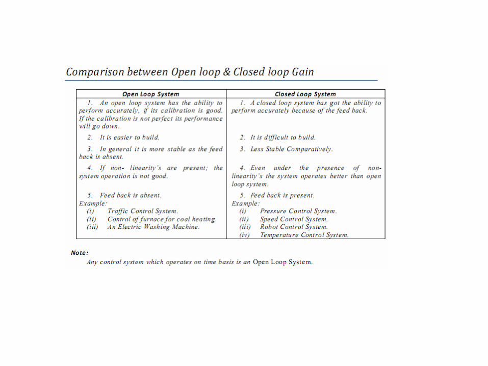
Examples of Modern Control Systems

Examples of Modern Control Systems

Examples of Modern Control Systems

Examples of Modern Control Systems

Examples of Modern Control Systems

Examples of Modern Control Systems

Examples of Modern Control Systems

Examples of Modern Control Systems

Examples of Modern Control Systems

The Future of Control Systems

Block diagram reduction

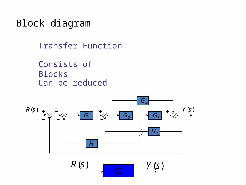
Block diagram

Transfer Function

Consists of Blocks

Can be reduced

)(sR2G 3G1G

4G

1H

2H

)(sY

G )(sY)(sR

Reduction techniques

2G1G 21GG

2. Moving a summing point behind a block

G G

G

1G

2G21 GG

1. Combining blocks in cascade or in parallel

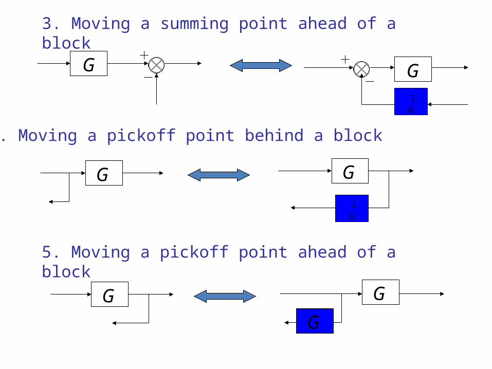
5. Moving a pickoff point ahead of a block

G G

G G

G1

G

3. Moving a summing point ahead of a block

G G

G1

4. Moving a pickoff point behind a block

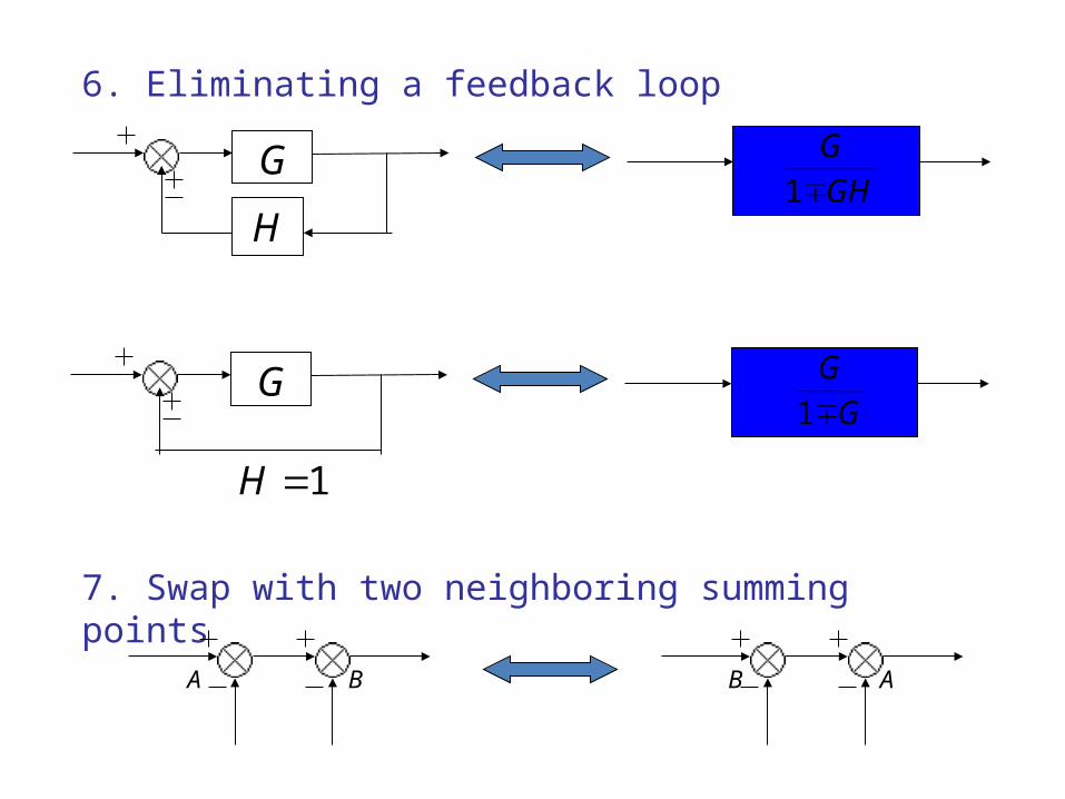
6. Eliminating a feedback loop

G

HGHG

1

7. Swap with two neighboring summing points

A B AB

G

1H

GG1

Example 1

Find the transfer function of the following block diagrams

2G 3G1G

4G

1H

2H

)(sY)(sR

(a)

1. Moving pickoff point A ahead of block 2G

2. Eliminate loop I & simplify

324 GGG B

1G

2H

)(sY4G

2G

1H

AB3G

2G

)(sR

I

Solution:

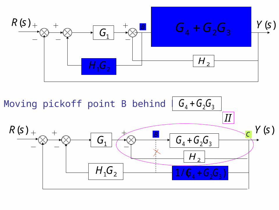
3. Moving pickoff point B behind block 324 GGG

1GB)(sR

21GH 2H

)(sY

)/(1 324 GGG

II

1GB)(sR C

324 GGG

2H

)(sY

21GH

4G

2G A3G 324 GGG

4. Eliminate loop III

)(sR)(1

)(

3242121

3241

GGGHHGGGGGG

)(sY

)()(1)(

)()()(

32413242121

3241

GGGGGGGHHGGGGGG

sRsYsT

)(sR1G

C

324

12

GGGHG

)(sY324 GGG

2H

C

)(1 3242

324

GGGHGGG

Using rule 6

2G1G

1H 2H

)(sR )(sY

3H

(b)

Solution:

1. Eliminate loop I

2. Moving pickoff point A behind block22

2

1 HGG

1G

1H

)(sR )(sY

3H

BA

22

2

1 HGG

2

221G

HG

1G

1H

)(sR )(sY

3H

2G

2H

BA

II

I

22

2

1 HGG

Not a feedback loop

)1(2

2213 G

HGHH

3. Eliminate loop II

)(sR )(sY22

21

1 HGGG

2

2213

)1(G

HGHH

21211132122

21

1)()()(

HHGGHGHGGHGGG

sRsYsT

Using rule 6

2G 4G1G

4H

2H

3H

)(sY)(sR

3G

1H

(c)

Solution:

2G 4G1G

4H)(sY

3G

1H

2H

)(sRA B

3H4

1G

4

1G

I1. Moving pickoff point A behind block 4G

4

3

GH

4

2

GH

2. Eliminate loop I and Simplify

II

III

443

432

1 HGGGGG

1G)(sY

1H

B

4

2

GH

)(sR

4

3

GH

II

332443

432

1 HGGHGGGGG

III

4

142

GHGH

Not feedbackfeedback

)(sR )(sY

4

142

GHGH

332443

4321

1 HGGHGGGGGG

3. Eliminate loop II & IIII

143212321443332

4321

1)()()(

HGGGGHGGGHGGHGGGGGG

sRsYsT

Using rule 6

3G1G

1H

2H

)(sR )(sY

4G

2G AB

(d)

Solution:

1. Moving pickoff point A behind block 3G I

1H3

1G

)(sY1G

1H

2H

)(sR

4G

2G A B

3

1G

3G

2. Eliminate loop I & Simplify

3G

1H

2G B

3

1G

2H

32GG B

23

1 HGH

1G)(sR )(sY

4G3

1

GH

23212

32

1 HGGHGGG

II

)(sR )(sY12123212

321

1 HGGHGGHGGGG

3. Eliminate loop II

12123212

3214 1)(

)()(HGGHGGHG

GGGGsRsYsT

4G

2G1G

4G

R Y

1H

3G

N

Determine the effect of R and N on Y in the following diagram

Example 2

NTRTYYY 2121

If we set N=0, then we can get Y1:

RTYY N 101

The same, we set R=0 and Y2 is also obtained:

NTYY R 202

Thus, the output Y is given as follows:

0021 RN YYYYY

In this linear system, the output Y contains two parts, one part is related to R and the other is caused by N:

Solution:

1. Swap the summing points A and B

2. Eliminate loop II & simplify

Y12

2

1 HGG

1G

4G

R

N

AB

3G

12

2131 1 HG

GGGG

R Y

N4G

II

3. Let N=0

RHGGGGGGGHG

HGGGGGGGY1321312112

132131211 1

12

2131 1 HG

GGGG

R Y

12

2131 1 HG

GGGG

R Y

N4G

o o

1YWe can easily get

Rewrite the diagram:

5. Break down the summing point M:

12

421431 1 HG

GGGGGG

YN

12

2131 1 HG

GGGG

4. Let R=0, we can get:

12

2131 1 HG

GGGG

4G

YN

M

])1(

)[(1

1

1432143142112

132131211321312112

21

NHGGGGGGGGGGHG

RHGGGGGGGHGGGGGGGHG

YYY

7. According to the principle of superposition, and can be combined together, So:

1Y 2Y

6. Eliminate above loops:

YN 12

421431 1

1HGGGGGGG

12

2131 1

1

1

HGGGGG

NHGGGGGGGHG

HGGGGGGGGGGHGY1321312112

14321431421122 1

1

Signal Flow Graph

What is Signal Flow Graph? SFG is a diagram which represents a set of simultaneous equations. This method was developed by S.J.Mason. This method does n’t require any reduction technique. It consists of nodes and these nodes are connected by a directed line called branches. Every branch has an arrow which represents the flow of signal. For complicated systems, when Block Diagram (BD) reduction method becomes tedious and time consuming then SFG is a good choice.

Comparison of BD and SFG

)(sR)(sG

)(sC )(sG

)(sR )(sC

block diagram: signal flow graph:

In this case at each step block diagram is to be redrawn. That’s why it is tedious method.So wastage of time and space.

Only one time SFG is to be drawn and then Mason’s gain formula is to be evaluated.So time and space is saved.

SFG

Node: It is a point representing a variable. x2 = t 12 x1 +t32 x3

X2

X1 X2

X3t12

t32

X1

Branch : A line joining two nodes.

Input Node : Node which has only outgoing branches.

X1 is input node.

In this SFG there are 3 nodes.

Definition of terms required in SFG

Output node/ sink node: Only incoming branches.

Mixed nodes: Has both incoming and outgoing branches.

Transmittance : It is the gain between two nodes. It is generally written on the branch near the arrow.

t12

X1

t23

X3

X4X2

t34

t43

• Path : It is the traversal of connected branches in the direction of branch arrows, such that no node is traversed more than once.• Forward path : A path which originates from the input node and terminates at the output node and along which no node is traversed more than once.• Forward Path gain : It is the product of branch transmittances of a forward path.

P 1 = G1 G2 G3 G4, P 2 = G5 G6 G7 G8

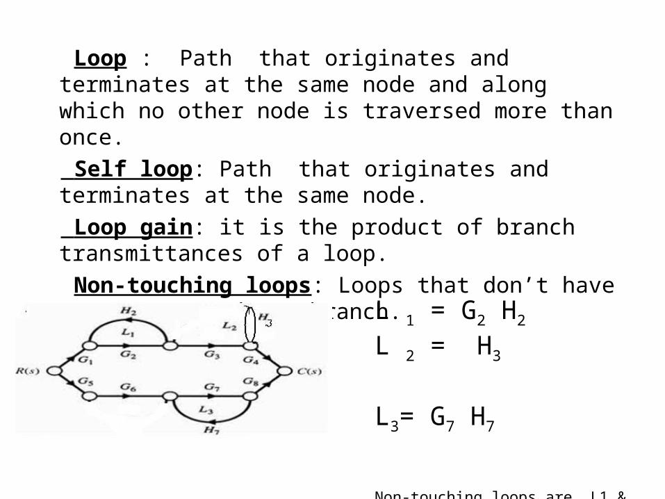
Loop : Path that originates and terminates at the same node and along which no other node is traversed more than once.

Self loop: Path that originates and terminates at the same node.

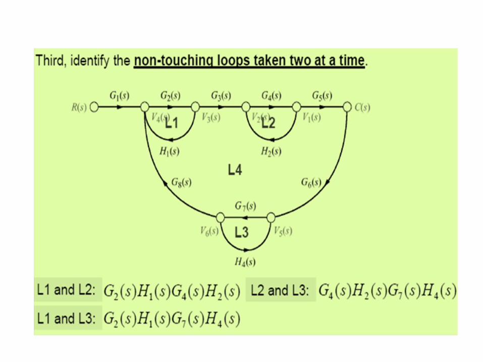
Loop gain: it is the product of branch transmittances of a loop. Non-touching loops: Loops that don’t have any common node

or branch.

L 1 = G2 H2 L 2 = H3

L3= G7 H7

Non-touching loops are L1 & L2, L1 &

L3, L2 &L3

SFG terms representation

input node (source)

b1x a

2x c

4x

d1

3x3x

mixed node mixed node

forward path

path

loop

branch

node

transmittance input node (source)

Rules for drawing of SFG from Block diagram

• All variables, summing points and take off points are represented by nodes.

• If a summing point is placed before a take off point in the direction of signal flow, in such a case the summing point and take off point shall be represented by a single node.

• If a summing point is placed after a take off point in the direction of signal flow, in such a case the summing point and take off point shall be represented by separate nodes connected by a branch having transmittance unity.

Mason’s Gain Formula

• A technique to reduce a signal-flow graph to a single transfer function requires the application of one formula.

• The transfer function, C(s)/R(s), of a system represented by a signal-flow graph is

k = number of forward path Pk = the kth forward path gain

∆ = 1 – (Σ loop gains) + (Σ non-touching loop gains taken two at a time) – (Σ non-touching loop gains taken three at a time)+ so on .

∆ k = 1 – (loop-gain which does not touch the forward path)

Ex: SFG from BD

EX: To find T/F of the given block diagram

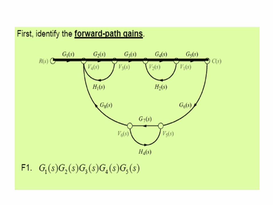
Identification of Forward Paths

P 1 = 1.1.G1 .G 2 . G3. 1= G1 G2 G3

P 2 = 1.1.G 2 . G 3 . 1= G 2 G3

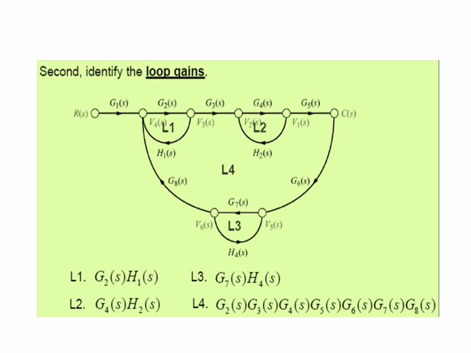
Individual Loops

L 1 = G 1G 2 H 1 L 2 = - G 2G 3 H 2

L 3 = - G 4 H 2

L 4 = - G 1 G 4

L 5 = - G 1 G 2 G 3

Construction of SFG from simultaneous equations

t21 t 23

t3

1 t32 t33

After joining all SFG

SFG from Differential equations

xyyyy 253Consider the differential equation

Step 2: Consider the left hand terms (highest derivative) as dependant variable and all other terms on right hand side as independent variables.Construct the branches of signal flow graph as shown below:-1

-5-2

-3y

y

y y

x

(a)

Step 1: Solve the above eqn for highest order

yyyxy 253

y

x

y

y

y

1-2-5

-31/s

1/s1/s

Step 3: Connect the nodes of highest order derivatives to the lowest order der.node and so on. The flow of signal will be from higher node to lower node and transmittance will be 1/s as shown in fig (b)

(b)

Step 4: Reverse the sign of a branch connecting y’’’ to y’’, with condition no change in T/F fn.

Step5: Redraw the SFG as shown.

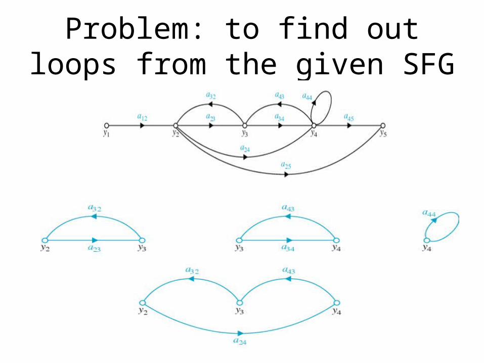
Problem: to find out loops from the given SFG

Ex: Signal-Flow Graph Models

P 1 =

P 2 =

Individual loops

L 1 = G2 H2

L 4 = G7 H7

L 3 = G6 H6

L 2= G3 H3

Pair of Non-touching loops L 1L 3 L 1L 4

L2 L3 L 2L 4

..)21(1( LiLjLkiLjLLL

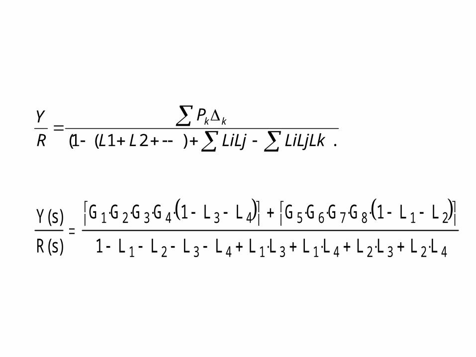
PRY kk

Y s( )R s( )

G 1 G 2 G 3 G 4 1 L 3 L 4 G 5 G 6 G 7 G 8 1 L 1 L 2

1 L 1 L 2 L 3 L 4 L 1 L 3 L 1 L 4 L 2 L 3 L 2 L 4

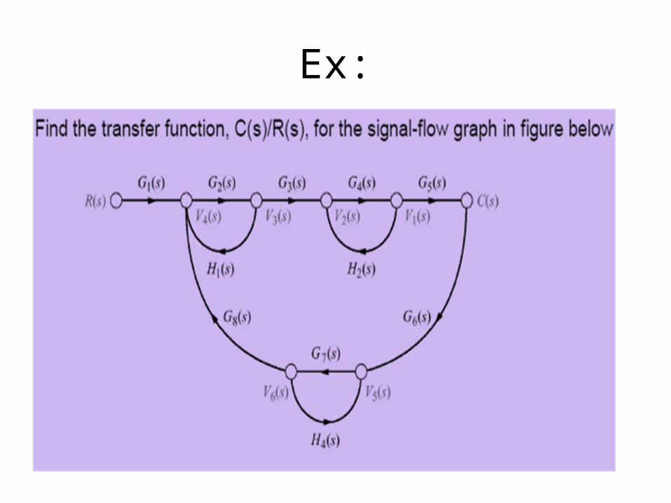
Ex:

Forward Paths

L5 = -G 4 H 4

L1= -G 5 G 6 H 1

L 3 = -G 8 H 1

L 2 = -G2 G 3G 4G 5 H2

L 4 = - G2 G 7 H2

Loops

Loops

L 7 = - G 1G2 G 7G 6 H3

L 6 = - G 1G2 G 3G 4G 8 H3

L 8= - G 1G2 G 3G 4G 5 G 6 H3

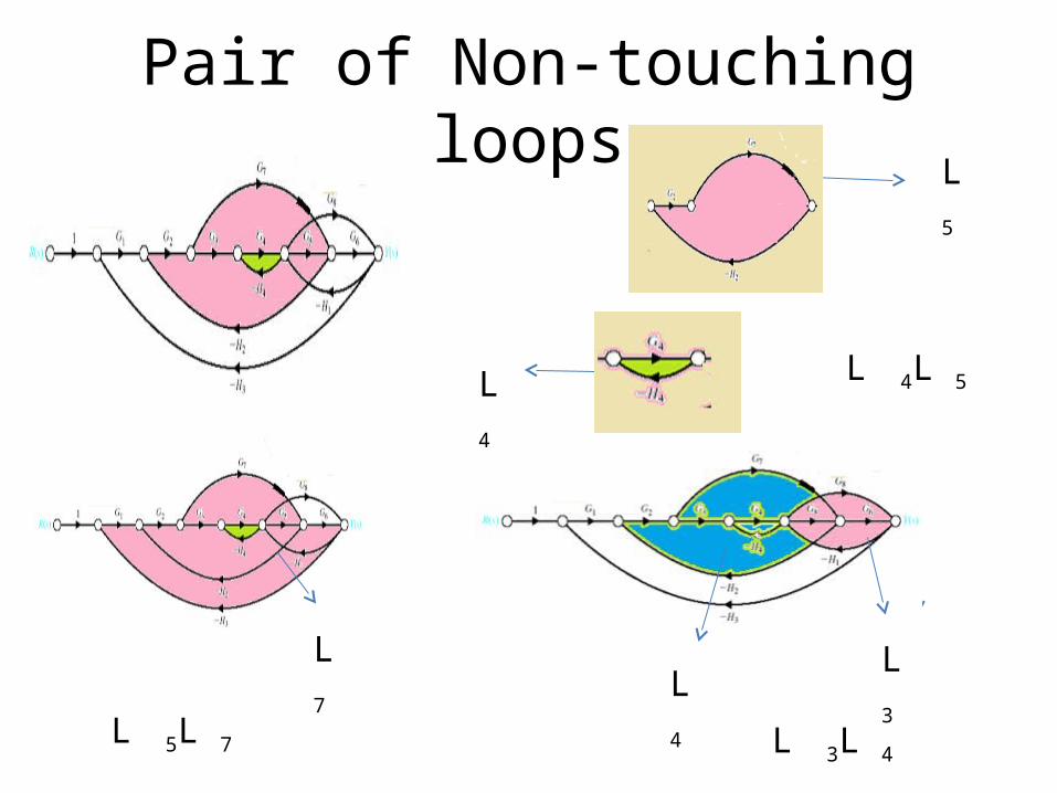
Pair of Non-touching loops

L 4

L 5

L 3L 7

L 4

L 5L 7

L 4L 5

L 3L 4

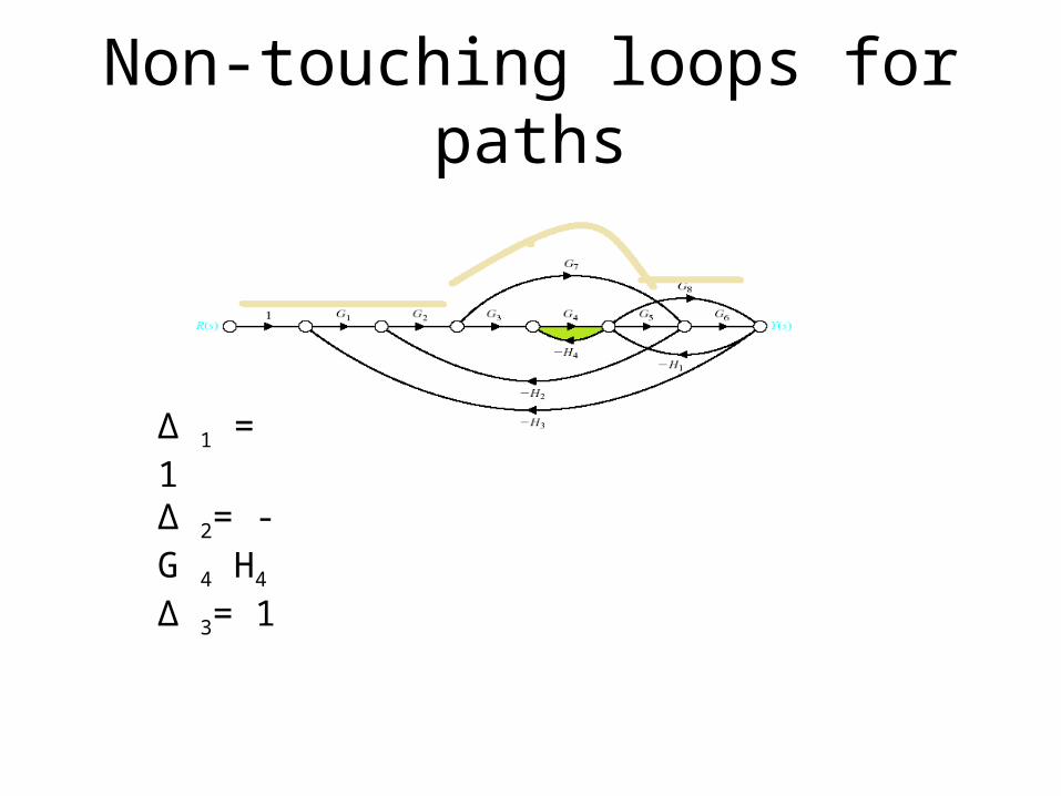
Non-touching loops for paths

∆ 1 = 1∆ 2= -G

4 H4

∆ 3= 1

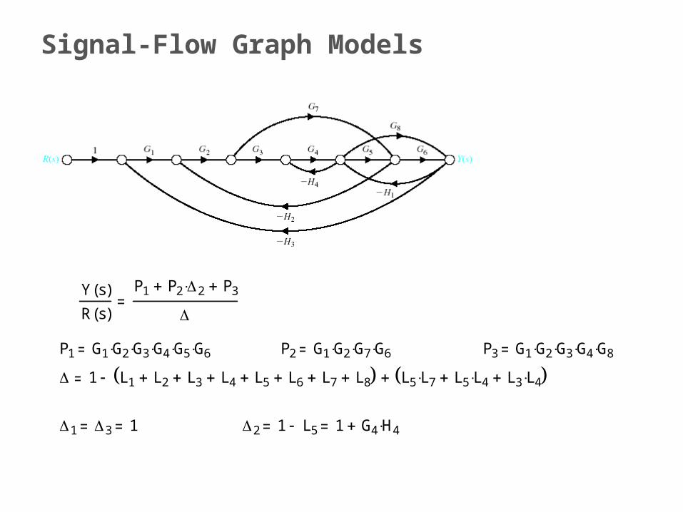
Signal-Flow Graph Models

Y s( )R s( )

P1 P2 2 P3

P1 G1 G2 G3 G4 G5 G6 P2 G1 G2 G7 G6 P3 G1 G2 G3 G4 G8

1 L1 L2 L3 L4 L5 L6 L7 L8 L5 L7 L5 L4 L3 L4

1 3 1 2 1 L5 1 G4 H4

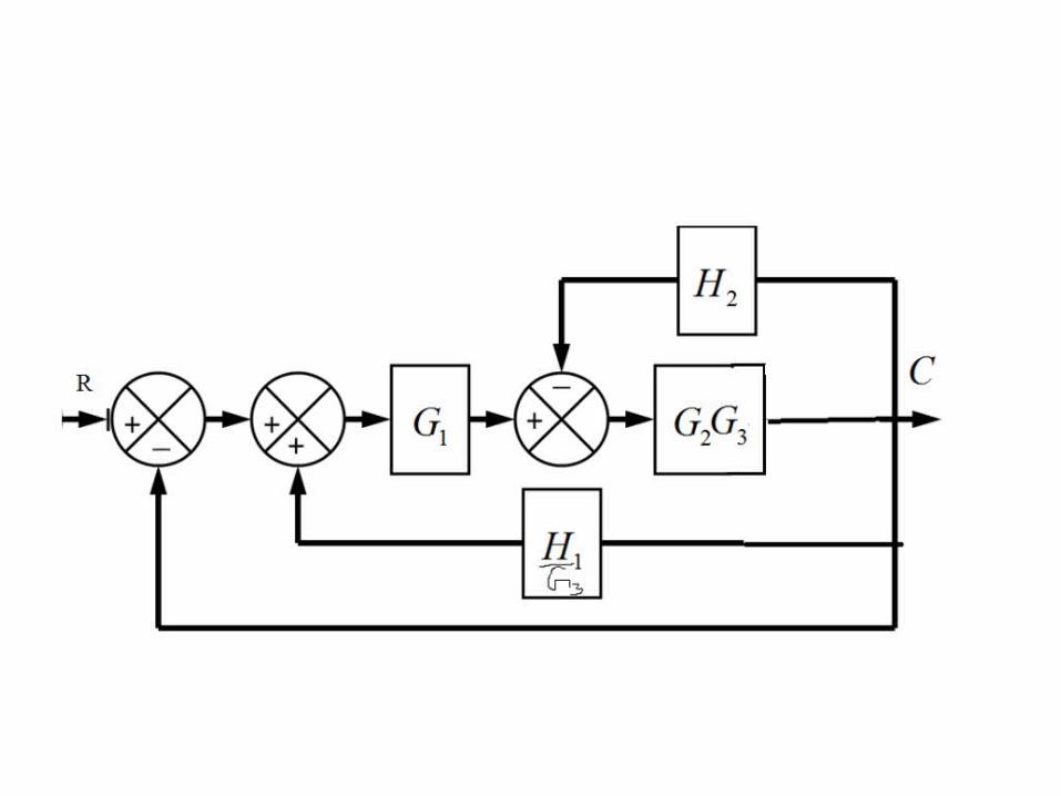
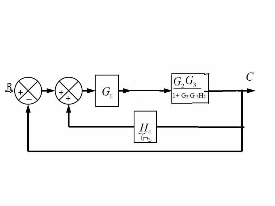
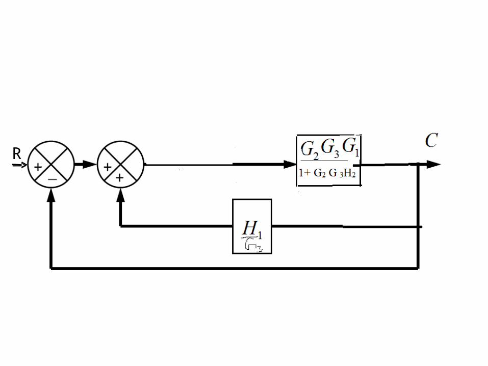
Block Diagram Reduction Example

R_+

_+1G 2G 3G

1H

2H

++

C

R

R

R

R_+

232121

321

1 HGGHGGGGG

C

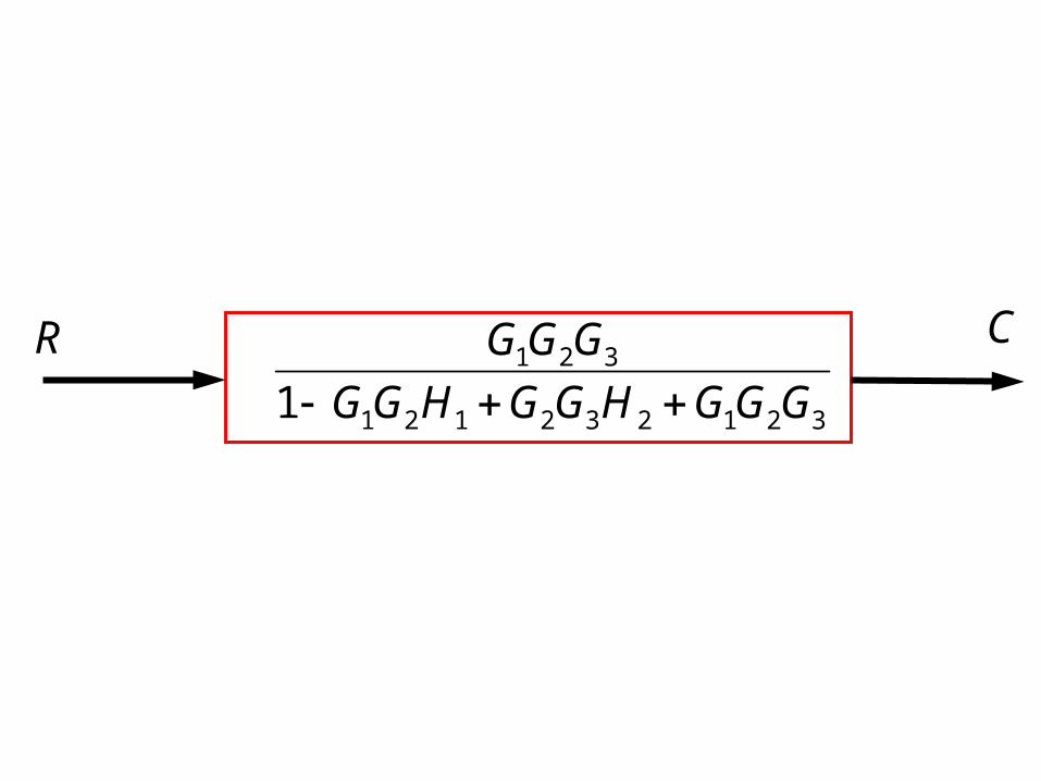
R

321232121

321

1 GGGHGGHGGGGG

C

Solution for same problem by using SFG

Forward Path

P 1 = G 1 G 2 G3

Loops

L 1 = G 1 G 2 H1 L 2 = - G 2 G3 H2

P 1 = G 1 G 2 G3

L 1 = G 1 G 2 H1

L 2 = - G 2 G3 H2

L 3 = - G 1 G 2 G3

∆1 = 1∆ = 1- (L1 + L 2 +L 3 )T.F= (G 1 G 2 G3 )/ [1 -G 1 G 2 H1 + G 1 G 2 G3 + G 2 G3 H2 ]

SFG from given T/F

( ) 24( ) ( 2)( 3)( 4)

C sR s s s s

)21()2(1

1

1

ss

s

Ex:

Example of block diagram

Step 1: Shift take off point from position before a block G4 to position after block G4

Step2 : Solve Yellow block.

Step3: Solve pink block.

Step4: Solve pink block.