UNIT III Tutorial 11: Predicting Precipitates and Maximum Ion Concentration

9/24/2004 Stat 567: Unit 8 - Ramón V. León 1
Unit 8: Maximum Likelihood for Location-Scale Distributions
Notes largely based on “Statistical Methods for Reliability Data”
by W.Q. Meeker and L. A. Escobar, Wiley, 1998 and on their class notes.
Ramón V. León

9/24/2004 Stat 567: Unit 8 - Ramón V. León 2
Unit 8 Objectives• Illustrate likelihood-based methods for
parametric models based on log-location-scale distributions (especially Weibull and Lognormal)
• Construct and interpret likelihood-ratio-based confidence intervals/regions for model parameters and for functions of model parameters
• Construct and interpret normal-approximation confidence intervals/regions
• Describe the advantages and pitfalls of assuming that the log-location-scale distribution shape parameter is known

9/24/2004 Stat 567: Unit 8 - Ramón V. León 3
Refresher

9/24/2004 Stat 567: Unit 8 - Ramón V. León 4
Weibull Probability Plot of the Shock Absorber Data

9/24/2004 Stat 567: Unit 8 - Ramón V. León 5
Weibull Distribution Likelihood for Right Censored Data

9/24/2004 Stat 567: Unit 8 - Ramón V. León 6
Lognormal Distribution Likelihood for Right Censored Data

9/24/2004 Stat 567: Unit 8 - Ramón V. León 7

9/24/2004 Stat 567: Unit 8 - Ramón V. León 8
1010.
210.4 10
.6
log(
eta)
234567beta
00.
20.
40.
60.
81
Rel
ativ
e Li
kelih
ood
ShockAbsorber data Weibull Distribution Relative Likelihood
The approximate 95% likelihood confidence interval for mu is: 10.06 10.54 The approximate 95% likelihood confidence interval for beta is: 1.897 4.772

9/24/2004 Stat 567: Unit 8 - Ramón V. León 9

9/24/2004 Stat 567: Unit 8 - Ramón V. León 10
0.10.20.5
0.9
eta
beta
20000 24000 30000 36000
2
3
4
5
6
7
Sat Sep 18 21:15:34 EDT 2004
ShockAbsorber data Weibull Distribution Relative Likelihood
The approximate 95% likelihood confidence interval for mu is: 10.06, 10.54 The approximate 95% likelihood confidence interval for beta is: 1.897 4.772

9/24/2004 Stat 567: Unit 8 - Ramón V. León 11

9/24/2004 Stat 567: Unit 8 - Ramón V. León 12
.005.02
.1
.3
.7
5000 15000 25000
Smallest Extreme Value Probability Plot
.002.02
.1
.4
.7
5000 15000 25000
Normal Probability Plot
Distance
.001.05
.3
.6
.8
5000 15000 25000
Largest Extreme Value Probability Plot
.001
.005.03.2.7
6000 10000 16000 24000
Weibull Probability Plot
.0005.01.1.3.6
6000 10000 16000 24000
Lognormal Probability Plot
Distance
.0001.01.1.3.6
6000 10000 16000 24000
Frachet Probability Plot
Frac
tion
Faili
ng
ShockAbsorber data Probability Plots with ML Estimates and Pointwise 95% Confidence Intervals

9/24/2004 Stat 567: Unit 8 - Ramón V. León 13

9/24/2004 Stat 567: Unit 8 - Ramón V. León 14
Distance
.001
.003
.005
.01
.02
.03
.05
.1
.2
.3
.5
.7
.9
6000 8000 10000 12000 14000 18000 22000 26000
Frac
tion
Faili
ng
ShockAbsorber data with Weibull ML Estimate and Pointwise 95% Confidence Intervals
Weibull Probability Plot
Sat Sep 18 21:42:22 EDT 2004
etahat = 27719
betahat = 3.16

9/24/2004 Stat 567: Unit 8 - Ramón V. León 15

9/24/2004 Stat 567: Unit 8 - Ramón V. León 16
Distance
.0005.001.002
.005.01.02
.05
.1
.2
.3
.4
.5
.6
.7
.8
6000 8000 10000 12000 14000 18000 22000 26000
Frac
tion
Failin
g
ShockAbsorber data Lognormal Probability Plot
Sat Sep 18 21:52:08 EDT 2004
Lognormal Distribution ML FitWeibull Distribution ML Fit95% Pointwise Confidence Intervals

9/24/2004 Stat 567: Unit 8 - Ramón V. León 17
Distance
.001
.003
.005
.01
.02
.03
.05
.1
.2
.3
.5
.7
.9
6000 8000 10000 12000 14000 18000 22000 26000
Frac
tion
Faili
ng
ShockAbsorber data Weibull Probability Plot
Sat Sep 18 21:46:22 EDT 2004
Weibull Distribution ML FitLognormal Distribution ML Fit95% Pointwise Confidence Intervals
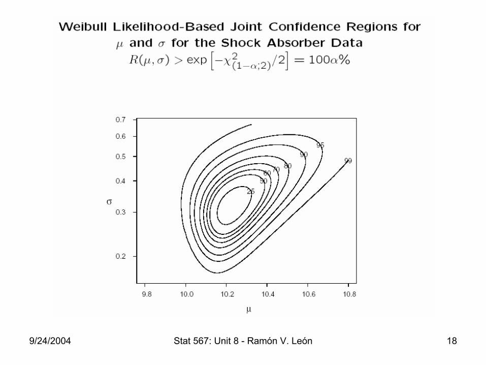
9/24/2004 Stat 567: Unit 8 - Ramón V. León 18

9/24/2004 Stat 567: Unit 8 - Ramón V. León 19
50
95
95
eta
beta
20000 24000 30000 36000
2
3
4
5
6
7
Sat Sep 18 21:56:52 EDT 2004
ShockAbsorber data Weibull Distribution Joint Confidence Region

9/24/2004 Stat 567: Unit 8 - Ramón V. León 20

9/24/2004 Stat 567: Unit 8 - Ramón V. León 21

9/24/2004 Stat 567: Unit 8 - Ramón V. León 22
0.0
0.2
0.4
0.6
0.8
1.0
10.0 10.2 10.4 10.6
Pro
file
Like
lihoo
d
mu
ShockAbsorber data Profile Likelihood and 95% Confidence Interval
for mu from the Weibull Distribution
Con
fiden
ce L
evel
0.99
0.95
0.90
0.80
0.70
0.60
0.50
Sat Sep 18 21:59:29 EDT 2004

9/24/2004 Stat 567: Unit 8 - Ramón V. León 23

9/24/2004 Stat 567: Unit 8 - Ramón V. León 24
0.0
0.2
0.4
0.6
0.8
1.0
2 3 4 5 6 7
Pro
file
Like
lihoo
d
beta
ShockAbsorber data Profile Likelihood and 95% Confidence Interval
for beta from the Weibull Distribution
Con
fiden
ce L
evel
0.99
0.95
0.90
0.80
0.70
0.60
0.50
Sat Sep 18 22:00:18 EDT 2004
( ) ( )( )
,ˆˆ ,
LR Max
Lµ
µ ββ
µ β=

9/24/2004 Stat 567: Unit 8 - Ramón V. León 25

9/24/2004 Stat 567: Unit 8 - Ramón V. León 26

9/24/2004 Stat 567: Unit 8 - Ramón V. León 27

9/24/2004 Stat 567: Unit 8 - Ramón V. León 28
1000012000
1400016000180002000022000
0.1 Quantile
Distance
2
3
4
56
7
beta
00.
20.
40.
60.
81
Rel
ativ
e Li
kelih
ood
ShockAbsorber data Weibull Distribution Relative Likelihood

9/24/2004 Stat 567: Unit 8 - Ramón V. León 29
50
95
0.1 Quantile Distance
beta
8000 12000 16000 20000
2
3
4
5
6
7
Sat Sep 18 22:25:18 EDT 2004
ShockAbsorber data Weibull Distribution Joint Confidence Region

9/24/2004 Stat 567: Unit 8 - Ramón V. León 30

9/24/2004 Stat 567: Unit 8 - Ramón V. León 31

9/24/2004 Stat 567: Unit 8 - Ramón V. León 32
0.0
0.2
0.4
0.6
0.8
1.0
8000 10000 12000 14000 16000 18000 20000 22000
Pro
file
Like
lihoo
d
0.1 Quantile Distance
ShockAbsorber data Profile Likelihood and 95% Confidence Interval
for 0.1 Quantile Distance from the Weibull Distribution
Con
fiden
ce L
evel
0.99
0.95
0.90
0.80
0.70
0.60
0.50
Sat Sep 18 22:25:18 EDT 2004

9/24/2004 Stat 567: Unit 8 - Ramón V. León 33

9/24/2004 Stat 567: Unit 8 - Ramón V. León 34
Maximum Likelihood Estimation in JMP 5:
Shock Absorber Data
(Compare results to those of
Table 8.1, Page 178 of your textbook)

9/24/2004 Stat 567: Unit 8 - Ramón V. León 35

9/24/2004 Stat 567: Unit 8 - Ramón V. León 36
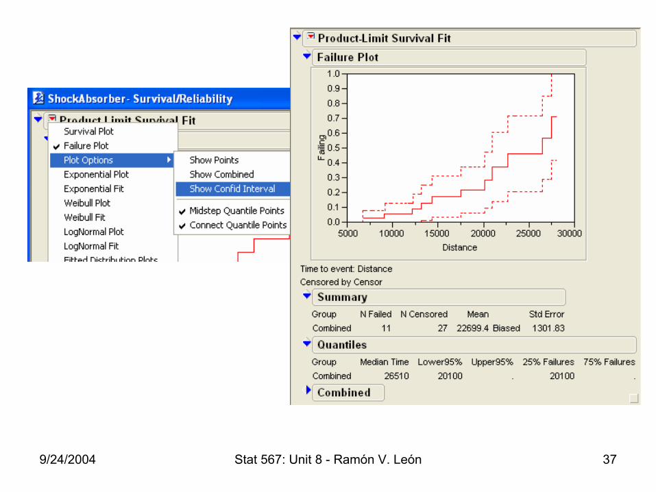
9/24/2004 Stat 567: Unit 8 - Ramón V. León 37

9/24/2004 Stat 567: Unit 8 - Ramón V. León 38
Compare estimates herewith those on Table 8.1 of the textbook

9/24/2004 Stat 567: Unit 8 - Ramón V. León 39
Maximum Likelihood in JMP
1 2
1 2
Let , ,..., be either failure times or right-censoredtimes (removal times). Define censoring codes , ,..., as follows:
0 if is a failure time1 if is a removal time
Then the li
n
n
ii
i
t t t
c c ct
ct
=
( ) ( ) ( )1
1
kelihood can be written as:
, ,i in c c
i ii
L f t S tθ θ θ−
=
= ∏

9/24/2004 Stat 567: Unit 8 - Ramón V. León 40
Maximum Likelihood in JMP: Loss
( ) ( )( ) ( )( )1
The negative of the loglikelihood is:
- 1 log ( , log ,n
i i i ii
l c f t c S tθ θ θ=
= − − + − ∑
JMP calls this kernel the “loss” function associated with maximum likelihood estimation
log ( , ) if 0log ( , ) otherwise
i i
i
f t closs
S tθθ
− == −

9/24/2004 Stat 567: Unit 8 - Ramón V. León 41
JMP Loss Examples: Exponential Case
log log if 0
log otherwise
i
i
t
ii
ti
te c
loss
te
θ
θ
θθ θ
θ
−
−
− = + = = − =

9/24/2004 Stat 567: Unit 8 - Ramón V. León 42
JMP Loss Example: Weibull/Gumbel Case
( )
( )
The Gumbel survival function is:
exp exp -
The Gumbel density function is:
exp( )
xS x x
x
f x S x
µσ
µσ
σ
− = − ∞ < < ∞
− = ×

9/24/2004 Stat 567: Unit 8 - Ramón V. León 43
JMP Loss Example: Weibull/Gumbel Case
log exp if 0
exp otherwise
ix x c
lossx
µ µσσ σ
µσ
− − − + = = −
log ( , ) if 0log ( , ) otherwise
i i
i
f t closs
S tθθ
− == −

9/24/2004 Stat 567: Unit 8 - Ramón V. León 44

9/24/2004 Stat 567: Unit 8 - Ramón V. León 45

9/24/2004 Stat 567: Unit 8 - Ramón V. León 46

9/24/2004 Stat 567: Unit 8 - Ramón V. León 47
Compare with resultson Table 8.1 of your textbook.
9/24/2004 Stat 567: Unit 8 - Ramón V. León 48
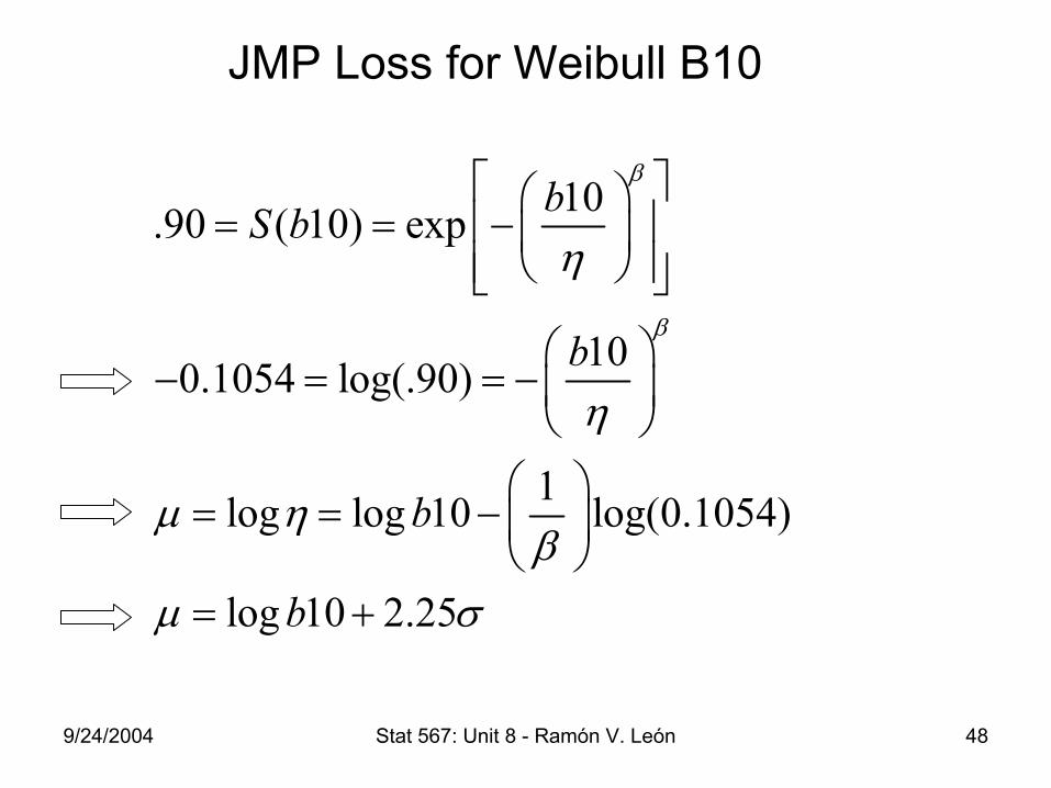
JMP Loss for Weibull B10
10.90 ( 10) exp
100.1054 log(.90)
1log log 10 log(0.1054)
log 10 2.25
bS b
b
b
b
β
β
η
η
µ ηβ
µ σ
= = −
− = = −
= = −
= +

9/24/2004 Stat 567: Unit 8 - Ramón V. León 49
JMP Loss for Weibull B10
log 10 2.25
log exp if 0
exp otherwise
i
b
x x closs
x
µ σ
µ µσσ σ
µσ
= +
− − − + = = −

9/24/2004 Stat 567: Unit 8 - Ramón V. León 50
JMP Using Local Variables

9/24/2004 Stat 567: Unit 8 - Ramón V. León 51

9/24/2004 Stat 567: Unit 8 - Ramón V. León 52
Compare to Table 8.1of your textbook

9/24/2004 Stat 567: Unit 8 - Ramón V. León 53
JMP loss for Weibull F(10,000)
( )[ ]( )
[ ]( )
1
( ) exp
log log log log ( )
log log log 1 ( )
log10000 log log 1 (10000)
tS t
t S t
t F t
F
β
β
η
η
µ σ
µ σ
= −
= − −
= − − −
= − − −

9/24/2004 Stat 567: Unit 8 - Ramón V. León 54
JMP loss for Weibull F(10,000)
[ ]( )log10000 log log 1 (10000)
log exp if 0
exp otherwise
i
F
x x closs
x
µ σ
µ µσσ σ
µσ
= − − −
− − − + = = −

9/24/2004 Stat 567: Unit 8 - Ramón V. León 55
Formula Using Local Variables

9/24/2004 Stat 567: Unit 8 - Ramón V. León 56

9/24/2004 Stat 567: Unit 8 - Ramón V. León 57
Compare to Table 8.1of your textbook

9/24/2004 Stat 567: Unit 8 - Ramón V. León 58
Exercises • Fit the exponential model to the Shock
Absorber data and calculate the MLEs for theta, b10, and F(10,000)
• Fit lognormal model to the Shock Absorber data and calculate the MLEs for theta, b10, and F(10,000)

9/24/2004 Stat 567: Unit 8 - Ramón V. León 59

9/24/2004 Stat 567: Unit 8 - Ramón V. León 60

9/24/2004 Stat 567: Unit 8 - Ramón V. León 61

9/24/2004 Stat 567: Unit 8 - Ramón V. León 62

9/24/2004 Stat 567: Unit 8 - Ramón V. León 63

9/24/2004 Stat 567: Unit 8 - Ramón V. León 64
( ) ( )cov ,,
( ) ( )X Y
cor X Yse X se Y
=

9/24/2004 Stat 567: Unit 8 - Ramón V. León 65

9/24/2004 Stat 567: Unit 8 - Ramón V. León 66
TrivariateDelta
Method( )
1 2 3
1 2 322 2
2
11 22 331 2 3
12 13 231 2 1 3 2 3
11 12 13
21 22 23
31
( , , )ˆ ˆ ˆ ˆ( , , )
ˆ
2
where
V=
g
g
g g gse v v v
g g g g g gv v v
v v vv v vv
φ θ θ θ
φ θ θ θ
φθ θ θ
θ θ θ θ θ θ
=
=
∂ ∂ ∂ = + + + ∂ ∂ ∂ ∂ ∂ ∂ ∂ ∂ ∂
+ + ∂ ∂ ∂ ∂ ∂ ∂
12 2 2
21 1 2 1 3
2 2 2
22 1 2 2 3
32 33 2 2 2
23 1 3 1 3
1 2 3ˆ ˆ ˆThe derivatives are evaluated at the MLEs , , ,
V is the variance-covar
l l l
l l l
v vl l l
θ θ θ θ θ
θ θ θ θ θ
θ θ θ θ θ
θ θ θ
− −∂ −∂ −∂ ∂ ∂ ∂ ∂ ∂ −∂ −∂ −∂ = ∂ ∂ ∂ ∂ ∂ −∂ −∂ −∂ ∂ ∂ ∂ ∂ ∂
iance matrix, and is the loglikelihood.l

9/24/2004 Stat 567: Unit 8 - Ramón V. León 67

9/24/2004 Stat 567: Unit 8 - Ramón V. León 68

9/24/2004 Stat 567: Unit 8 - Ramón V. León 69

9/24/2004 Stat 567: Unit 8 - Ramón V. León 70

9/24/2004 Stat 567: Unit 8 - Ramón V. León 71
DMBA Carcinogen Data(Data from Pike, 1966. See Lawless, 1982)
Number of days until the appearance of vaginal carcinoma in n = 19 female rats painted with carcinogen DMBA
143, 164, 188, 188, 190, 192, 206, 209, 213, 216, 220, 227, 230, 234, 246, 265, 304, 216*, 244*
By the end of the study only 17 out of the 19 rats had developed carcinoma, so that two of the times (marked *) are censoring times.

9/24/2004 Stat 567: Unit 8 - Ramón V. León 72

9/24/2004 Stat 567: Unit 8 - Ramón V. León 73

9/24/2004 Stat 567: Unit 8 - Ramón V. León 74
IUD Data(Data from WHO, 1987)
Number of weeks from the moment of initial IUD use until discontinuation because of bleeding problems in n = 18 women
10, 13*, 18*, 19, 23*, 30, 36, 38*, 54*, 56*, 59, 75, 93, 97, 104*, 107, 107*, 107*
By the end of the study only 9 out of the 18 women had developed bleeding, so that 9 of the times (marked *) are censoring times.

9/24/2004 Stat 567: Unit 8 - Ramón V. León 75

9/24/2004 Stat 567: Unit 8 - Ramón V. León 76

9/24/2004 Stat 567: Unit 8 - Ramón V. León 77

9/24/2004 Stat 567: Unit 8 - Ramón V. León 78
Derivation
11
1 2
1 2
If is Wei( , ), then is Exp( ) since
( ) exp exp .
It follows that if , ,..., are Wei( , ) failure or removal times,
then , ,..., are Exp(n
n
T T
t tP T t P T t
T T T
T T T
β β
β
ββ β
β
β β β
η β η
η η
η β
> = > = − = −
) failure or removal times.βη

9/24/2004 Stat 567: Unit 8 - Ramón V. León 79
( )
1
1
1
1
1 1 1
1 1 1
Now for the exponential estimates (with
ˆstandard error ) so that estimates .
1Also
n
ii
n
nii
ii
n n n
i i ii i i
t
r
tt
rrr
t t tse se
r r
β
β
β ββ
β ββ β β
η
η η
β
=
=
=
−
= = =
=
=
∑
∑∑
∑ ∑ ∑
( )1 1 1
1
1 1
ˆ1 1 1 1
n
n nii
i ii i
r
tt t
rr r r rr
ββ ββ β
ηβ β β
−
=
= =
=
= =
∑∑ ∑

9/24/2004 Stat 567: Unit 8 - Ramón V. León 80

9/24/2004 Stat 567: Unit 8 - Ramón V. León 81

9/24/2004 Stat 567: Unit 8 - Ramón V. León 82

9/24/2004 Stat 567: Unit 8 - Ramón V. León 83

9/24/2004 Stat 567: Unit 8 - Ramón V. León 84
Component B Safe-Life Data

9/24/2004 Stat 567: Unit 8 - Ramón V. León 85

9/24/2004 Stat 567: Unit 8 - Ramón V. León 86

9/24/2004 Stat 567: Unit 8 - Ramón V. León 87

9/24/2004 Stat 567: Unit 8 - Ramón V. León 88