Unifying the inertia and Riemann curvature tensors through geometric algebraM. Berrondo, J. Greenwald, and C. Verhaaren Citation: American Journal of Physics 80, 905 (2012); doi: 10.1119/1.4734014 View online: http://dx.doi.org/10.1119/1.4734014 View Table of Contents: http://scitation.aip.org/content/aapt/journal/ajp/80/10?ver=pdfcov Published by the American Association of Physics Teachers

This article is copyrighted as indicated in the article. Reuse of AAPT content is subject to the terms at: http://scitation.aip.org/termsconditions. Downloaded to IP:

128.187.97.22 On: Wed, 12 Feb 2014 03:50:37

Unifying the inertia and Riemann curvature tensors through geometricalgebra

M. Berrondo,a) J. Greenwald,b) and C. Verhaarenc)

Department of Physics and Astronomy, Brigham Young University, Provo, Utah 84602

(Received 24 September 2009; accepted 22 June 2012)

We follow a common thread to express linear transformations of vectors and bivectors from

different fields of physics in a unified way. The tensorial representations are coordinate independent

and assume a compact form using Clifford products. As specific examples, we present (a) the inertia

tensor as a vector-to-vector as well as a bivector-to-bivector linear transformation; (b) the

Newtonian tidal acceleration; and (c) the Riemann tensor corresponding to a Schwarzschild black

hole as a bivector-to-bivector tensorial transformation. The resulting expressions have a remarkable

similarity when expressed in terms of geometric products. VC 2012 American Association of Physics Teachers.

[http://dx.doi.org/10.1119/1.4734014]

I. INTRODUCTION

Geometric algebras (also called Clifford algebras) areused to endow physical spaces with a useful algebraic struc-ture. By analyzing the physical system within this context,we can find alternative interpretations of the underlyingphysics.1,2 These can simplify computational problems inaddition to giving us much more compact and clean notation.In most cases, the final results can be expressed in acoordinate-free way.

An algebra is constructed by endowing a linear space withan additional binary operation called the product of the alge-bra. Although this product is usually non-commutative, it isdistributive with respect to the linear space addition, and it isassumed to be associative for our case. With these rules, theidea of matrix multiplication immediately comes to mind. Itwill actually be useful to keep this picture in mind, as long aswe conceive of the algebra’s sum and product in an abstractway. An additional and essential condition for the algebra isclosure with respect to its product, i.e., the complete algebramust contain all possible products of its elements. Again, inour matrix multiplication reference, this would imply choos-ing square matrices of fixed size: a product of two n� n mat-rices is again an n� n matrix, in addition to the fact that alinear combination of matrices is again a matrix.

Geometric algebras constitute a specific instance of asso-ciative algebras. The constraint imposed on their structureallows us to give concrete geometric interpretations to boththe elements and the operations within the algebra.1,3 In asense, this is the natural extension of the Cartesian concep-tion of identifying geometry and algebra, and unifying theminto a single structure. The geometric building blocks arepoints, vectors, oriented surfaces, and oriented volumes. Thealgebraic part relates them in a constructive way and allowsus to unify both concepts and equations from different fieldsof physics.

Our aim in this work is to apply these tools to four specificexamples: the inertia tensor interpreted as (i) a second ranktensor and (ii) a fourth rank tensor; (iii) the second rank tidalacceleration tensor; and (iv) the fourth rank Weyl tensor.The main object is to find a common form of expressing allthese linear transformations in a coordinate-free way bytaking advantage of the Clifford product as well as its intrin-sic geometric interpretation. Second rank tensors appear asvector to vector mappings, while the specific fourth ranktensors in our examples map bivectors to bivectors. A further

simplification in all these examples arises from the use ofsymmetry: we consider the case of an axisymmetric rigidbody to calculate explicitly the inertia tensor, and we assumespherical symmetry for both the non-relativistic tidal acceler-ation and the curvature tensor for the Schwarzschild blackhole examples.

Section II introduces the main concepts of geometric alge-bras, as well as the notation that we will need in this work.In particular, we define the algebra associated to the Euclid-ean three-dimensional space, known as the Pauli algebra.Section III deals with the inertia tensor for a rigid body. Theexample of a simple rod is presented and the inertia tensor iswritten in terms of the geometric product as a vector-valuedlinear transformation of vectors. This is followed by the caseof a general axisymmetric body with equivalent expressions.Section IV derives the tidal acceleration for the Newtoniancase and the corresponding tensor is shown to have a similarform. In Section V, we present a parallel development interms of mappings between bivectors for the case of the iner-tia tensor first and for the Weyl conformal tensor as a gener-alization of the tidal acceleration. Section VI includes someconclusions regarding the unifying power of geometric alge-bras in physics.

II. PAULI ALGEBRA

A. Geometric product of vectors

We first want to build up the geometric algebra startingfrom a physical vector space V regarded as an underlyingpart of the larger linear space of the algebra G. We also needto admit a metric defined by the usual dot product of twovectors a; b 2 V

a � b ¼ ab cos h; (1)

where a and b are the magnitudes of the vectors and h is theangle between them. This operation forces us to include thereal numbers R as a linear subspace of G, providing the Clif-ford algebra with a graded structure where the scalars havegrade 0 and the physical vector space V has grade 1. Wenext find the elements of grade 2, called bivectors, by form-ing the “wedge” (or exterior, or Grassmann4 product ^) oftwo vectors, thus encoding the plane defined by them. Giventhat two collinear vectors do not form a plane, a ^ a ¼ 0:Taking advantage of the distributivity rule,

905 Am. J. Phys. 80 (10), October 2012 http://aapt.org/ajp VC 2012 American Association of Physics Teachers 905

This article is copyrighted as indicated in the article. Reuse of AAPT content is subject to the terms at: http://scitation.aip.org/termsconditions. Downloaded to IP:

128.187.97.22 On: Wed, 12 Feb 2014 03:50:37

ðaþ bÞ ^ ðaþ bÞ ¼ a ^ bþ b ^ a ¼ 0; (2)

we obtain the antisymmetry property of the wedge product

a ^ b ¼ �b ^ a: (3)

Furthermore, the area of the parallelogram formed by thetwo vectors is abjsin hj, so the bivector represents an orientedsurface (see Fig. 1).

Clifford’s stroke of genius5 converted Schwartz’s inequal-ity (for both the dot and wedge products) to an equality bydefining the geometric product of two vectors a and b in Vas

ab ¼ a � bþ a ^ b (4)

and then building up the geometric algebra by demandingclosure. This geometric product combines zero-grade scalarswith second-grade bivectors with a resulting magnitude6

kabk ¼ ab: (5)

Thus, geometric algebras constrain the symmetric part of theproduct of two vectors to correspond to their dot product, as isevident in Eq. (4). The antisymmetric part of this product isassociative, making the geometric product itself associative.1,2

In order to close the algebra, we need to keep incorporat-ing new multivectors of higher grade. The wedge product oftwo vectors gives a bivector; bivectors can now be wedgedwith another vector to produce a trivector, and so on. Theseadditional structures represent oriented volumes (and hyper-volumes), as illustrated in Fig. 1 and will eventually closethe algebra in a finite number of steps due to the antisymme-try property, Eq. (3). With this geometric interpretation, thewedge product turns out to be associative.1,2,4 Because oftheir geometric liaison, multivectors are also very useful forinterpreting the behaviors of many familiar physical quanti-ties as we will show below.

B. Geometric algebra in 3-d

Our main example is the Clifford algebra G3 generated bythe three-dimensional Euclidean space V ¼ R3. This Paulialgebra7 is eight dimensional and consists of linear combina-tions of multivectors of grades 0 to 3, i.e., scalars, 3-dvectors, 3-d bivectors, and 1-d trivectors (also called pseudo-scalars). The basis element of the real line R is the number1. For R3, we choose an orthonormal basis of unit vectors,e1; e2; e3. The advantage of using orthonormality is that wecan rely on the more versatile Clifford product in order to

construct the subsequent multivector bases. For instance, thebivector basis element e1 ^ e2 turns out to be the same as theproduct e1e2 in this case. The eight basis elements of thePauli algebra are classified by grades in Table I.

Notice that the three resulting unit bivectors square to �1instead of 1. This follows from their antisymmetry; forexample,

e1e2 ¼ e1 ^ e2 ¼ �e2 ^ e1 ¼ �e2e1; (6)

and hence ðe1e2Þ2 ¼ e1e2e1e2 ¼ �ðe1e1Þðe2e2Þ ¼ �1. Thesame is true for the pseudo-scalar (unit trivector)

ðe1e2e3Þ2 ¼ e1e2e3e1e2e3 ¼ �1: (7)

It can also be appreciated from Fig. 1 that the unit trivec-tor e1e2e3 represents the (right handed) oriented unit cube.At the same time, we can use Eq. (7), together with the factthat the unit trivector commutes with all the basis elements,to identify it with the imaginary unit i (in an algebraic sense).This is the actual meaning of the third column in Table I.

In summary, we can take i as the basis element of the triv-ectors, and fiekg as the basis of the bivectors, for the Paulialgebra. In other words, every vector a 2 R3 has a corre-sponding dual bivector A ¼ ia, and vice versa, a ¼ –iA.This duality associates a vector a normal to the surfacedefined by the bivector A in a natural way (see Appendix).

For the present example G3, the duality property isexpressed as

a ^ b ¼ ia� b; (8)

in terms of the unit pseudo-scalar i. Two main features dis-tinguish Grassmann’s wedge product from Gibbs’s crossproduct:

(a) the ^ is well defined for any number of dimensions (aswell as for pseudo-Euclidean spaces) and

(b) the ^ is associative while the � fulfills Jacobi’sidentity.

For the particular case of the Pauli algebra, we can thusrewrite the defining Eq. (4) as

ab ¼ a � bþ ia� b; (9)

in terms of the usual dot and cross products between twothree-dimensional vectors.

C. Problem for students

Using the duality results for the Pauli algebra stated in theAppendix show that for any three vectors a; b; c 2 R3,

a ^ b ^ c ¼ ia � ðb� cÞ; (10)

and give the geometric interpretation of this result.

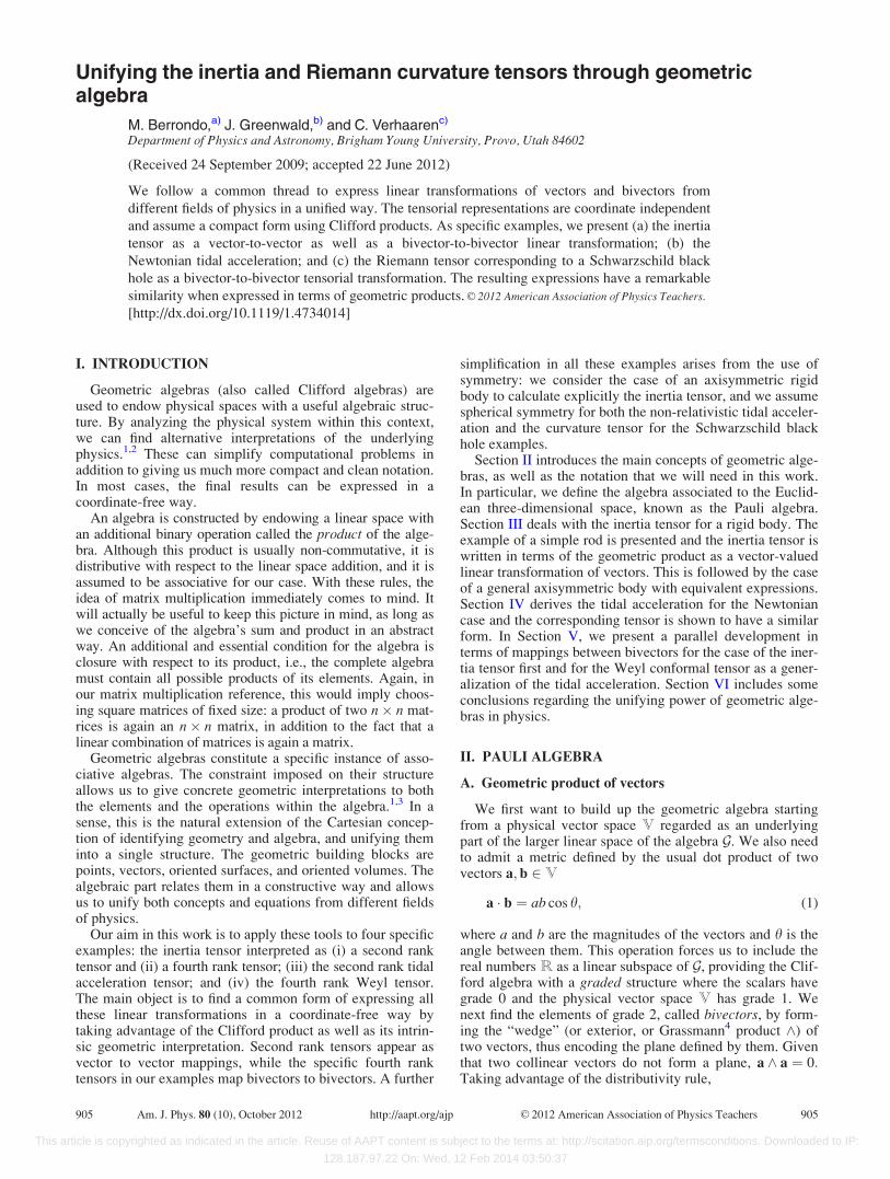
Fig. 1. The wedge product of two vectors a, b is an oriented area, while the

wedge of a, b, c is an oriented volume.

Table I. The graded algebraic structure.

Grade Basis “Complex form” Space

0 1 1 R

1 e1; e2; e3 e1; e2; e3 R3

2 e1e2; e2e3; e3e1 ie1; ie2; ie3 iR3

3 e1e2e3 i iR

906 Am. J. Phys., Vol. 80, No. 10, October 2012 Berrondo, Greenwald, and Verhaaren 906

This article is copyrighted as indicated in the article. Reuse of AAPT content is subject to the terms at: http://scitation.aip.org/termsconditions. Downloaded to IP:

128.187.97.22 On: Wed, 12 Feb 2014 03:50:37

III. THE INERTIA TENSOR

A. Angular velocity and angular momentum pseudo-vectors

The classical mechanics formula for the angular momen-tum vector in terms of the mass m, the position vector r, andthe velocity v is L ¼ m r� v, with corresponding dualbivector L ¼ iL. For any particle rotating with angular ve-locity x, the tangential velocity is v ¼ x� r. Consider arigid body rotating about some axis (see Fig. 2). Each parti-cle will have the same angular velocity x. Using Eq. (8), thetotal angular momentum of the rigid body8 can be written interms of the Clifford product in Eq. (9) by summing over allthe particles k ¼ 1… N

L ¼XN

k

mkrk � ðx� rkÞ ¼ �iXN

k

mkrk ^ ðx� rkÞ

¼ �iXN

k

mkrkðx� rkÞ ¼XN

k

mkrkðrk ^ xÞ: ð11Þ

In the continuum limit, this becomes

L ¼ð

rðr ^ xÞ dm (12)

in terms of the mass distribution of the rigid body.The inertia tensor plays the role of the mass (tensor) for

rotational motion:9 the angular momentum vector L isobtained as the (scalar) product of the inertia tensor I withthe angular velocity vector x. In the language of Misner,Thorne, and Wheeler,10 I is a “one-slot” machine sendingvectors to vectors, so its matrix representation has two indi-ces. In other words, it is a linear mapping I : R3 ! R3, andhence L ¼ IðxÞ:8

Both the angular velocity x and the angular momentum Ltransform as pseudo-vectors (or axial vectors) with respect tospatial reflections and inversions. Thus, a better descriptionof them is given in terms of their duals, the bivectorsX ¼ ix, and L ¼ iL, representing the corresponding planes(see Appendix). This relationship will be exploited in Sec.V A.

B. Moment of inertia: Example

Equation (12) defines the inertia tensor as a linear func-tion, i.e., given any vector A, the image vector B is given by

B ¼ IðAÞ ¼ð

r ðr ^ AÞ dm; (13)

and the matrix elements Ikl with respect to the given ortho-normal basis fekg can be extracted as the projections

Ikl ¼ ek � IðelÞ: (14)

This 3� 3 matrix fIklg is symmetric and includes themoments and products of inertia with respect to the originalbasis.

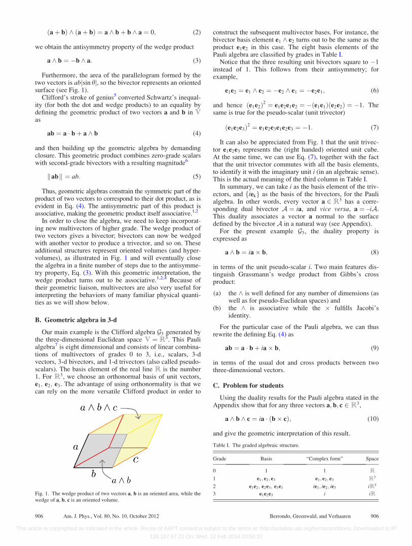
Let us now look at a concrete simple example. Using Eq.(12), it is straightforward to find the inertia tensor for a rotat-ing rod and write it in a coordinate-free way. Consider a thinrod of length a extending from �a/2 to a/2 and rotatingabout an arbitrary axis passing through its center (see Fig. 3).Choosing s as the integration variable, dm¼m ds/a, and r ¼sn in terms of the unit vector n along the rod, we have

IðxÞ ¼ða=2

�a=2

sn ðsn ^ xÞm ds

a¼ ma2

12nðn ^ xÞ: (15)

This result can be rewritten in terms of geometric productsonly, using n ^ x ¼ ðnx� xnÞ=2 from Eq. (4). This moresymmetric form,

IðAÞ ¼ ma2

24ðA� nAnÞ (16)

is actually the leit motif of the present work. Indeed the sec-ond term, A0 ¼ �nAn, has a simple geometric interpreta-tion:2,8 A0 corresponds to the vector A reflected with respectto the plane in.

C. Axially symmetric case

Let us next consider the more general case of an axiallysymmetric body rotating about an arbitrary axis x. Giventhat the inertia tensor is symmetric, it can be diagonalizedwith corresponding orthogonal eigenvectors. The eigenval-ues fI1; I2; I3g are real numbers and represent the principalmoments of inertia.9 Define ff1; f2; f3g as the respective unitvectors along the principal axes of the rigid body, andassume that f3 is the symmetry axis, so that the two momentsof inertia associated with the plane if3 are equal, i.e., I1 ¼ I2.

In the body-fixed basis (see Fig. 4), the inertia tensor canbe written in terms of the components of x as

Fig. 2. All points in a rigid body rotate about the rotation axis (here, indi-

cated by an �) at the same angular velocity, x. Fig. 3. A thin rod of length a rotating about its center at angular velocity x.

907 Am. J. Phys., Vol. 80, No. 10, October 2012 Berrondo, Greenwald, and Verhaaren 907

This article is copyrighted as indicated in the article. Reuse of AAPT content is subject to the terms at: http://scitation.aip.org/termsconditions. Downloaded to IP:

128.187.97.22 On: Wed, 12 Feb 2014 03:50:37

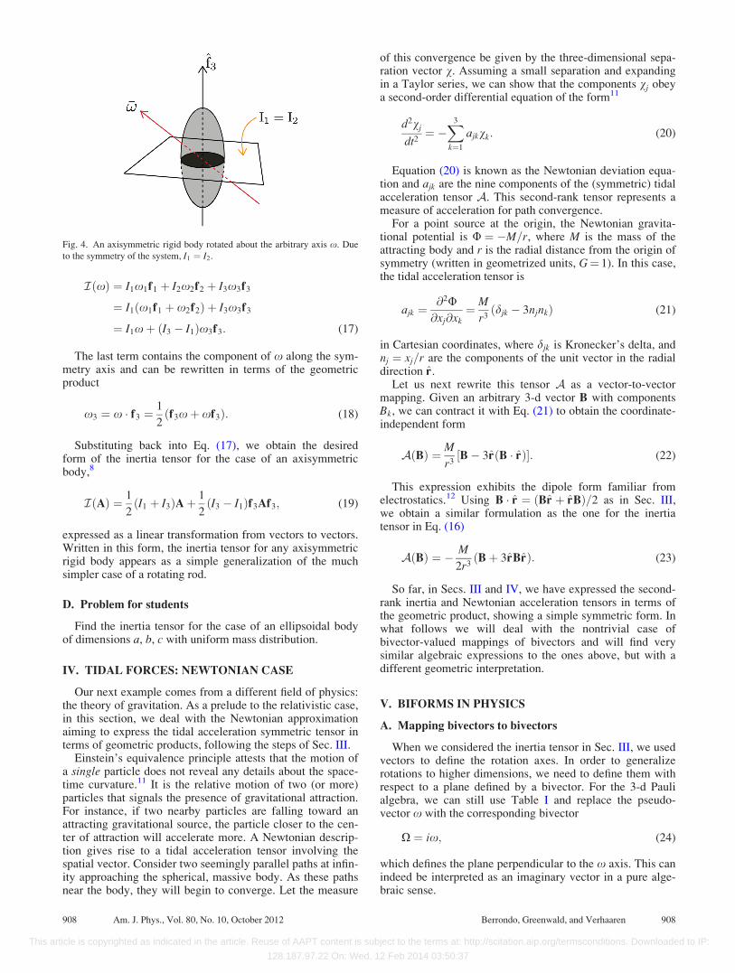
IðxÞ ¼ I1x1f1 þ I2x2f2 þ I3x3f3

¼ I1ðx1f1 þ x2f2Þ þ I3x3f3

¼ I1xþ ðI3 � I1Þx3f3: (17)

The last term contains the component of x along the sym-metry axis and can be rewritten in terms of the geometricproduct

x3 ¼ x � f3 ¼1

2ðf3xþ xf3Þ: (18)

Substituting back into Eq. (17), we obtain the desiredform of the inertia tensor for the case of an axisymmetricbody,8

IðAÞ ¼ 1

2ðI1 þ I3ÞAþ

1

2ðI3 � I1Þf3Af3; (19)

expressed as a linear transformation from vectors to vectors.Written in this form, the inertia tensor for any axisymmetricrigid body appears as a simple generalization of the muchsimpler case of a rotating rod.

D. Problem for students

Find the inertia tensor for the case of an ellipsoidal bodyof dimensions a, b, c with uniform mass distribution.

IV. TIDAL FORCES: NEWTONIAN CASE

Our next example comes from a different field of physics:the theory of gravitation. As a prelude to the relativistic case,in this section, we deal with the Newtonian approximationaiming to express the tidal acceleration symmetric tensor interms of geometric products, following the steps of Sec. III.

Einstein’s equivalence principle attests that the motion ofa single particle does not reveal any details about the space-time curvature.11 It is the relative motion of two (or more)particles that signals the presence of gravitational attraction.For instance, if two nearby particles are falling toward anattracting gravitational source, the particle closer to the cen-ter of attraction will accelerate more. A Newtonian descrip-tion gives rise to a tidal acceleration tensor involving thespatial vector. Consider two seemingly parallel paths at infin-ity approaching the spherical, massive body. As these pathsnear the body, they will begin to converge. Let the measure

of this convergence be given by the three-dimensional sepa-ration vector v. Assuming a small separation and expandingin a Taylor series, we can show that the components vj obeya second-order differential equation of the form11

d2vj

dt2¼ �

X3

k¼1

ajkvk: (20)

Equation (20) is known as the Newtonian deviation equa-tion and ajk are the nine components of the (symmetric) tidalacceleration tensor A. This second-rank tensor represents ameasure of acceleration for path convergence.

For a point source at the origin, the Newtonian gravita-tional potential is U ¼ �M=r, where M is the mass of theattracting body and r is the radial distance from the origin ofsymmetry (written in geometrized units, G¼ 1). In this case,the tidal acceleration tensor is

ajk ¼@2U@xj@xk

¼ M

r3ðdjk � 3njnkÞ (21)

in Cartesian coordinates, where djk is Kronecker’s delta, andnj ¼ xj=r are the components of the unit vector in the radialdirection r.

Let us next rewrite this tensor A as a vector-to-vectormapping. Given an arbitrary 3-d vector B with componentsBk, we can contract it with Eq. (21) to obtain the coordinate-independent form

AðBÞ ¼ M

r3½B� 3rðB � rÞ�: (22)

This expression exhibits the dipole form familiar fromelectrostatics.12 Using B � r ¼ ðBr þ rBÞ=2 as in Sec. III,we obtain a similar formulation as the one for the inertiatensor in Eq. (16)

AðBÞ ¼ � M

2r3ðBþ 3rBrÞ: (23)

So far, in Secs. III and IV, we have expressed the second-rank inertia and Newtonian acceleration tensors in terms ofthe geometric product, showing a simple symmetric form. Inwhat follows we will deal with the nontrivial case ofbivector-valued mappings of bivectors and will find verysimilar algebraic expressions to the ones above, but with adifferent geometric interpretation.

V. BIFORMS IN PHYSICS

A. Mapping bivectors to bivectors

When we considered the inertia tensor in Sec. III, we usedvectors to define the rotation axes. In order to generalizerotations to higher dimensions, we need to define them withrespect to a plane defined by a bivector. For the 3-d Paulialgebra, we can still use Table I and replace the pseudo-vector x with the corresponding bivector

X ¼ ix; (24)

which defines the plane perpendicular to the x axis. This canindeed be interpreted as an imaginary vector in a pure alge-braic sense.

Fig. 4. An axisymmetric rigid body rotated about the arbitrary axis x. Due

to the symmetry of the system, I1 ¼ I2.

908 Am. J. Phys., Vol. 80, No. 10, October 2012 Berrondo, Greenwald, and Verhaaren 908

This article is copyrighted as indicated in the article. Reuse of AAPT content is subject to the terms at: http://scitation.aip.org/termsconditions. Downloaded to IP:

128.187.97.22 On: Wed, 12 Feb 2014 03:50:37

On the other hand, we also know that the angular momen-tum L behaves as a vector with respect to rotations but notwith respect to inversions or reflections. We saw in Sec. IIIthat angular momentum can also be correctly described as abivector. We thus define the bivector

L ¼ r ^ p ¼ ir� p ¼ iL: (25)

For the case of a rigid body, we have to integrate over themass distribution (or sum over all the particles in the discretecase) as in Eq. (12)

L ¼ i

ðrðr ^ xÞ dm ¼ i

ð1

2ðr2x� rxrÞ dm

¼ð

1

2ðr2X� rXrÞ dm: (26)

Using Eq. (A3) from the Appendix, the first line in theequation above can be rewritten in terms of the angular ve-locity bivector X ¼ ix as

L ¼ð

rðr �XÞ dm;¼ �ð

rðX � rÞ dm (27)

involving the contraction of the vector r with the bivector X,which turns out to be antisymmetric (see Appendix).

The inertia tensor now becomes a biform,13 i.e., abivector-valued linear transformation of bivectors. Thus, theinertia tensor I is reinterpreted as mapping the plane definedby a bivector B to a new plane C

C ¼ IðBÞ ¼ð

rðr � BÞ dm ¼ð

1

2ðr2B � rBrÞ dm: (28)

This in turn leads directly to the analogue of Eq. (19),

L ¼ IX ¼ I1 þ I3

2Xþ I3 � I1

2f3Xf3; (29)

as a mapping from bivectors to bivectors for the axisymmet-ric case. We would like to emphasize that although this lastequation looks almost identical to Eq. (19), they are concep-tually different. While the latter refers to a second rank ten-sor mapping vectors to vectors, Eq. (29) is a biform, i.e., abivector-valued transformation of a bivector.

B. The Riemann curvature tensor

The following three subsections make up a series of steppingstones aiming to express the Weyl conformal tensor as abiform using geometric products.2 In Sec. V B we give a gen-eral introduction to curvature, the Riemann curvature tensor,and its relation with the Weyl tensor.10 In Sec. V C we concen-trate on the latter’s specific properties, while Sec. V D relatesboth curvature tensors to general relativity for the case of theSchwarzschild solution.

We usually think of a surface as being curved from theway it warps or bends in our 3-d space. Let us suppose thatwe are constrained to a curved 2-d surface, such as the sur-face of a sphere, without access to the third dimension. Inthis case, we would like to be able to determine whether ornot our surface is curved in an intrinsic fashion. A way toquantify this is to calculate the curvature tensor (or Riemanntensor). It allows us to extend the notion of curvature to

(a) more than two dimensions;(b) each point in the curved space;(c) different directions; and(d) Lorentzian metrics.

The Riemann tensor R accounts for the rotation of a vec-tor as it travels along a closed path while always pointing inthe same direction. The more the transported vector differsfrom the original one, the larger the curvature. On a planarsurface, it is easy to set the pointing direction of any vectorand keep it fixed as we travel along a circle or a square. Theresulting vector points in the same direction as the original,there is no net rotation, and hence the curvature vanishes in-dependently of the chosen direction and the chosencoordinates.

For the more general case of a higher dimensional curvedspace, we need to follow an infinitesimal path in order toobtain the local curvature at each point.14 The chosen smallclosed path defines a two-dimensional surface. We could, forinstance, choose two coordinates u and v and form a four-sided (oriented) loop of sides Du and Dv. Let us next choosea vector X and parallel-transport it along the closed loop tothe rotated final vector X0. The bivectors u ^ X andv ^ X

0define two different planes. The Riemann tensor maps

one bivector onto the second bivector. In other words, thecurvature tensor R, in any number of dimensions d � 2, is alinear biform mapping bivectors to bivectors

R : bivectors! bivectors: (30)

Hence, R is a fourth-rank tensor.In the theory of general relativity, the Riemann tensor R

can be considered as a “tidal acceleration” tensor10 general-izing the corresponding Newtonian tensor appearing in Eq.(20) to the 4-d curved space-time.

A more restricted measure of the curvature is given by theWeyl conformal tensorW. It measures the tidal accelerationtaken along a geodesic and detects only the distortion of theshape of the body but carries no information on its change ofvolume. Indeed it is the only part of the curvature that existsin free space. In two and three dimensions, the Weyl tensorvanishes identically. In four or more dimensions, W corre-sponds to the traceless part of the Riemann tensor R. Thedifference between these two tensors is expressed in terms ofthe second-rank Ricci tensor mapping 4-d vectors to 4-dvectors.10

In order to study the Riemann tensor and its trace in fourdimensions, we would have to consider the corresponding16-dimensional algebra instead of the more limited 8-dimensional Pauli algebra. However, given the special prop-erties of W, it is possible and convenient to express it interms of a combination of vectors and bivectors of the Paulialgebra. The more complete derivation starting from a space-time split of bivectors15 and considering biforms within the16-dimensional Dirac algebra is given in detail elsewhere.2

In this paper, we exploit the fact that the Pauli algebra is iso-morphic to the even subalgebra of the Dirac algebra.15

C. The Weyl tensor

In Sec. III, we found the principal moments as the eigen-values of the inertia tensor I . Given that this transformationis real and symmetric, there is no question about its threeeigenvalues being real. Knowing these eigenvalues allowed

909 Am. J. Phys., Vol. 80, No. 10, October 2012 Berrondo, Greenwald, and Verhaaren 909

This article is copyrighted as indicated in the article. Reuse of AAPT content is subject to the terms at: http://scitation.aip.org/termsconditions. Downloaded to IP:

128.187.97.22 On: Wed, 12 Feb 2014 03:50:37

us to write I in a simple form, especially in the axisymmet-ric case. This is true even when we consider I as a biform,as in Eq. (29).

Our aim now is to generalize this procedure to the case ofa curvature biform in a four-dimensional curved space. Inthis case, the local (tangent) space turns out to be Minkowskispace, M4 ¼ R1;3. As is well known, the (1þ 3)-d flatspace-time of special relativity is Lorentzian, meaning thatthe “distance” Ds between two events (i.e., two points in thisspace) acquires a hyperbolic character

ðDsÞ2 ¼ c2ðDtÞ2 � ðDrÞ2; (31)

where r refers to vectors in the usual 3-d space.We now have six basis bivectors that can be separated into

two different types:

(a) three spatial bivectors corresponding to the three or-thogonal spatial planes whose square is �1 and

(b) three spatio-temporal planes where one of the definingaxes is time and whose square is þ1.

Strictly speaking, these six bivectors form part of the largerDirac algebra G1;3.15 However, if we choose the time axis tocoincide with the direction of the observer, we can iden-tify15,16 the set in (b) with the 3-d basis vectors in Table I,while (a) coincides with the 3-d bivectors fie1; ie2; ie3g. Fromthis point of view, Dirac bivectors correspond to Pauli“complex” vectors. Within this particular reference frame, itturns out to be sufficient to restrict ourselves to the G3 algebrain order to study Lorentz transformations and the Weyl con-formal tensor. As mentioned above, the Ricci tensor and thecomplete Riemann tensor require, in addition, the inclusion ofmappings between 4-d vectors absent in the Pauli algebra.

Incidentally, given the hyperbolic nature of Minkowskispace, we can also construct “null elements” whose squaresvanish (i.e., they are nilpotent), such as e16ie3. These turnout to play an important role in describing the paths followedby light and have been extensively used in the Newman-Penrose description of general relativity.17

In this paper, we shall follow a different path: instead ofconsidering six basis elements for the bivectors in the tan-gent M4 space, we restrict ourselves to a real 3-d vectorlocal basis fe1; e2; e3g and allow for “complex” coefficients.Within this frame, the biform corresponding to the Weylconformal tensor W can now be interpreted as a linear map-ping between complex 3-d vectors. In a way, this is a gener-alization of Sec. V A above where the inertia tensor appearedas a linear transformation between “imaginary” 3-d vectors.Although W is still symmetric as a linear transformation, itturns out to be complex symmetric so there is no longer aguarantee that the corresponding eigenvalues are real.

Regarding the application of these ideas to general relativ-ity, we can confine ourselves to the source-free case of Ein-stein’s equation where the Riemann tensor R coincides withthe Weyl tensorW. The reason is that the difference betweenthe two tensors involves the Ricci tensor, which vanishes inthis case.10

The Weyl tensor W has the following useful proper-ties2,10,18 as a linear transformation:

(a) W is complex symmetric;(b) W is traceless;(c) W is self-dual, i.e., WðiBÞ ¼ iWðBÞ for any complex

vector B.

In other words, W can be represented as a 3� 3 complexsymmetric, traceless matrix W with respect to the given 3-dbasis

Wkl ¼ Wlk;

TrðWÞ ¼ 0;

WðBÞ ¼X

kl

WklekBel: (32)

In analogy to the principal moments of inertia, we cansolve the eigenvalue problem,

WðVÞ ¼ kV: (33)

There are three complex eigenvalues fk1; k2; k3g associ-ated to each point of the curved space, with three corre-sponding eigenvectors fV1;V2;V3g. Given that W istraceless, the sum of the three eigenvalues vanishes so onlytwo of them are independent. Comparing with the inertiatensor in Sec. V A above, we notice that the complexeigenvectors include in general an additional real part, absentin the R3 case. This is indeed due to the presence ofadditional space-time planes in M4.

The particular case in which the three eigenvectors spanthe entire 3-d space14,17–19 is especially important from thepoint of view of Einstein’s general theory of relativity. Inother words, there are no null eigenplanes in this case andwe can choose three orthonormal (principal) vectors, V i ¼ f i

with f2i ¼ 1 for i¼ 1, 2, 3. First, let us assume that the three

eigenvalues are all different. Using the identity

Xi

f iBf i ¼ �B; (34)

valid for any complex vector B, and taking into account thetraceless nature of W, we can eliminate k3 and expand it13

using only two eigenvalues

WðBÞ ¼ f1Bf1 þ1

3B

� �G1 þ f2Bf2 þ

1

3B

� �G2; (35)

where G1 ¼ 2k1 þ k2 and G2 ¼ 2k2 þ k1 are functions ofthe space-time event depending on the curvature propertiesof the 1þ 3-dimensional curved space.

D. The Riemann tensor for the Schwarzschild solution

In Einstein’s theory of general relativity, the space-time de-pendent metric tensor10,11 is usually taken as the physicalobject, characterizing the gravitational system by defining ameasure of the space-time deformation. By the same token,the curvature tensor R is the crucial geometric componentand it plays the role of a gravitational field strength, given thata nonvanishing curvature tensor implies the presence of gravi-tation.20 The curvature tensor corresponds to the tidal acceler-ation tensor whose Newtonian limit is given by Eq. (20).

For the source-free case, R and W coincide. Thus, Eq.(35) above is a canonical form of the Riemann tensor for awhole class of solutions of Einstein vacuum equations.19 Inparticular, if there is a geometric symmetry involved, we canfollow the same procedure as in Sec. III for the inertia tensor.This will allow us to eliminate one more term in Eq. (35)and rewrite it as

910 Am. J. Phys., Vol. 80, No. 10, October 2012 Berrondo, Greenwald, and Verhaaren 910

This article is copyrighted as indicated in the article. Reuse of AAPT content is subject to the terms at: http://scitation.aip.org/termsconditions. Downloaded to IP:

128.187.97.22 On: Wed, 12 Feb 2014 03:50:37

WðBÞ ¼ Gðt; rÞ f1Bf1 þ1

3B

� �; (36)

where the explicit form of G is determined by the specificphysical problem.

The simplest nontrivial case is that of a static, sphericallysymmetric space-time. The Schwarzschild solution10,11 toEinstein’s vacuum equations follows from the following(somewhat redundant) premises:

(a) no time dependence of G;(b) spherical symmetry, G¼G(r);(c) behaves locally as M4; and(d) coincides asymptotically with the Newtonian case.

Following the ideas developed in Sec. III, we can nowchoose the unit principal vector f1 as corresponding to spher-ical symmetry, i.e., f1 ¼ r according to (b) above. The Rie-mann tensor for the Schwarzschild solution can be expressedas a biform in our now-familiar form2

RðBÞ ¼ WðBÞ ¼ � 3M

2r3rBr þ 1

3B

� �; (37)

where M is the black hole mass. It differs from Eq. (23) onlyin the fact that W maps tangent planes to tangent planes inthe curved space of general relativity instead of the simplerCartesian 3-d space.

VI. DISCUSSION

The geometric interpretation of bivectors as orientedsurfaces in Grassmann algebras becomes especially rele-vant in Minkowski 4-d space-time and associated curvedspaces, where we have to distinguish between purely spatialand time-space mixed surfaces. By including a metric andthe corresponding dot product in Clifford algebras, we canextend this geometric advantage to an algebraic one aswell. Bivectors in R3 can be treated as imaginary 3-d vec-tors eliciting a duality relation between both sets. Addingtime as a coordinate in Minkowski space M4 producesthree more planes with a hyperbolic geometry. The corre-sponding unit bivectors square to 1 (instead of �1) andhence can be identified with the R3 basis vectors, at least aslong as we choose the observer’s reference frame. Thisspace-time split15 allows us to refer all possible M4 bivec-tors to the Pauli algebra as defined in Table I. Algebrai-cally, we treat the linear combinations of the sixindependent Dirac bivector basis elements as complex 3-dvectors within G3. Thus, antisymmetric tensors (such as theelectromagnetic field) can be rewritten as complex 3-dvectors.15,16

The final expressions in Secs. III and IV are written interms of Clifford products. Given that they correspond to lin-ear mappings of vectors, they can be expressed in terms ofdot products as well, i.e., projecting the vector along the cho-sen fixed direction. Equations (17) and (22) have this form.In the case of biforms, i.e., tensors mapping bivectors tobivectors, this is not so simple given that the product of twobivectors is a linear combination of scalars, bivectors, andtetravectors corresponding to dot products, commutators,and wedge products.2 So, in this respect, Eqs. (29) and (35)are true canonical representations for the fourth-rank axi-symmetric inertia tensor and Weyl tensor for the cases con-sidered in this work.

APPENDIX: PSEUDO-VECTORS AND BIVECTORS

In the usual 3-d Euclidean geometry, the cross product oftwo vectors turns out to be a pseudo-vector in the sense thatthe resulting vector does not change sign with respect to aspatial inversion, while a regular vector does. Typicalexamples are the angular momentum, the torque, and themagnetic field. The angular velocity (being proportional tothe angular momentum in the simplest case) is also apseudo-vector.

The concept of a pseudo-vector can be generalized to anynumber of dimensions (and pseudo-Euclidean spaces) byshifting our geometric perspective. Instead of looking at thedirectional aspect of the pseudo-vector, we can conveythe same information by defining the bivector dual to thepseudo-vector. This bivector defines the plane perpendicularto the pseudo-vector. Unlike the concept of a pseudo-vector,the bivector (and its corresponding plane) is well defined inany number of dimensions. From the tensorial point of view,the bivector corresponds to a second-rank antisymmetrictensor.

For instance, in the case of the motion of a planet withconstant angular momentum L, its dual bivector L ¼ iLdefines the plane of planetary motion through the wedgeproduct, Eq. (25). The angular velocity bivector X in Eq.(24) thus describes the dynamics of the rotational motion ofa plane independently of the dimension of the vector space.

The wedge product and the dot product in Eq. (4) haveentirely different geometric interpretations and their alge-braic properties are also different. Hence, it is necessary toconsider the commutation relation of the pseudo-scalar iwith respect to each of them separately. In the specific caseof the Pauli algebra G3, i commutes with every element ofthe algebra with respect to the geometric product.21 How-ever, when we consider the dot and the wedge products ontheir own, this is no longer true. Indeed the duality relationof Eq. (8) can be generalized.2 Given two 3-d vectors a andb, we can consider the contraction of the vector a with thebivector bi

a � ðbiÞ ¼ ða ^ bÞi: (A1)

The result of this contraction (dot product) is a vector.This also shows explicitly that we cannot “pull out” i whendealing with the dot or the wedge product separately, in spiteof the fact that this is a valid operation with respect to thefull geometric product.

We also have that ðbiÞ � a ¼ ðb ^ aÞi ¼ �a � ðbiÞ, and ingeneral the dot product of a vector and a bivector isantisymmetric,

a � B ¼ �B � a; (A2)

instead of being symmetric as in the usual case of two vec-tors (a � b ¼ b � a).

For the wedge product, duality reads

a ^ ðbiÞ ¼ ða � bÞi; (A3)

confirming the fact that the wedge product of a vector with abivector is a pseudo-scalar in G3.

a)Electronic mail: berrondo@byu.edub)Electronic mail: Jared_Greenwald@Baylor.educ)Electronic mail: chrisverhaaren@gmail.com

911 Am. J. Phys., Vol. 80, No. 10, October 2012 Berrondo, Greenwald, and Verhaaren 911

This article is copyrighted as indicated in the article. Reuse of AAPT content is subject to the terms at: http://scitation.aip.org/termsconditions. Downloaded to IP:

128.187.97.22 On: Wed, 12 Feb 2014 03:50:37

1D. Hestenes, “Oersted medal lecture 2002: Reforming the mathematical

language of physics,” Am. J. Phys. 71, 104–121 (2003).2C. Doran and A. Lasenby, Geometric Algebra for Physicists (Cambridge

University Press, Cambridge, UK, 2003).3Clifford (Geometric) Algebras, edited by W. E. Baylis (Birkhauser,

Boston, 1996).4Hermann Gunther Grassmann, edited by G. Schubring (Kluwer,

Dordrecht, 1996).5W. K. Clifford, Mathematical Papers (MacMillan, London, 1882).6This property also allows (non-vanishing) vectors to be invertible with

respect to the Clifford product.7The well-known Pauli matrices form a representation of the basis elements

of R3 in terms of traceless Hermitian 2� 2 matrices.8D. Hestenes, New Foundations for Classical Mechanics (Kluwer,

Dordrecht, 1999).9J. B. Marion and S. T. Thornton, Classical Dynamics of Particles andSystems, 4th ed. (Harcourt Brace, Fort Worth, 1995).

10C. W. Misner, K. S. Thorne, and J. A. Wheeler, Gravitation (W. H. Free-

man, San Francisco, 1973).11J. B. Hartle, Gravity: An Introduction to Einstein’s General Relativity

(Addison-Wesley, San Francisco, 2003).

12D. J. Griffiths, Introduction to Electrodynamics, 3rd ed. (Prentice-Hall,

Englewood Cliffs, 1995).13D. Hestenes and G. Sobczyk, Clifford Algebra to Geometric Calculus

(Reidel, Dordrecht, 1984).14J. Snygg, Clifford Algebra: A Computational Tool for Physicists (Oxford

University Press, Oxford, UK, 1997).15D. Hestenes, “Spacetime physics with geometric algebra,” Am. J. Phys.

71, 691–714 (2003).16W. E. Baylis, Electrodynamics: A Modern Geometric Approach (Bir-

khauser, Boston, 1999).17R. Penrose and W. Rindler, Spinors and Space-Time (Cambridge Univer-

sity Press, Cambridge, UK, 1984).18M. R. Francis and A. Kosowsky, “Geometric algebra techniques for

general relativity,” Ann. Phys. 311, 459–502 (2004).19Known as Petrov type I case.20S. Weinberg, Gravitation and Cosmology: Principles and Applications of

the General Theory of Relativity (Wiley, New York, 1972), Chap. 6.21The pseudo-scalar commutes with all the elements for Clifford algebras

generated by odd-dimensional vector spaces. For even dimensions, the

pseudo-scalar anticommutes with odd-grade multivectors and commutes

with even-grade multivectors.

912 Am. J. Phys., Vol. 80, No. 10, October 2012 Berrondo, Greenwald, and Verhaaren 912

This article is copyrighted as indicated in the article. Reuse of AAPT content is subject to the terms at: http://scitation.aip.org/termsconditions. Downloaded to IP:

128.187.97.22 On: Wed, 12 Feb 2014 03:50:37