Understanding SDAIII Jitter Calculation...
12
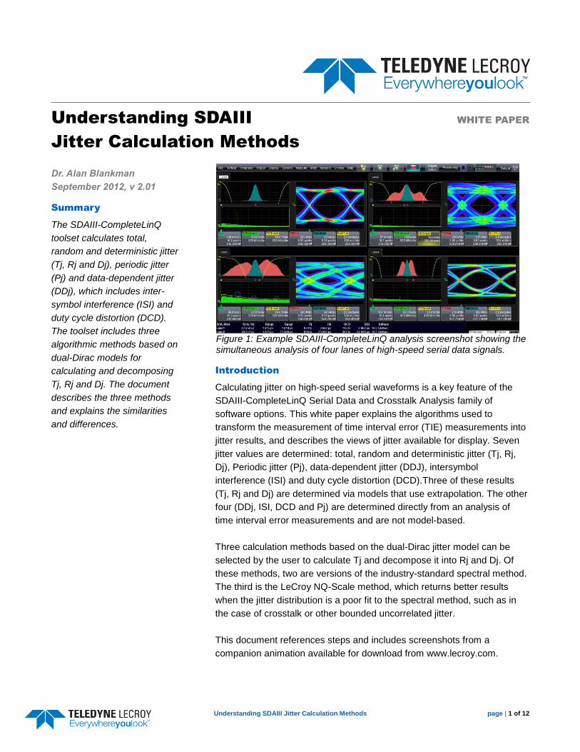
Understanding SDAIII Jitter Calculation Methods page | 1 of 12 Understanding SDAIII WHITE PAPER Jitter Calculation Methods Dr. Alan Blankman September 2012, v 2.01 Summary The SDAIII-CompleteLinQ toolset calculates total, random and deterministic jitter (Tj, Rj and Dj), periodic jitter (Pj) and data-dependent jitter (DDj), which includes inter- symbol interference (ISI) and duty cycle distortion (DCD). The toolset includes three algorithmic methods based on dual-Dirac models for calculating and decomposing Tj, Rj and Dj. The document describes the three methods and explains the similarities and differences. Introduction Calculating jitter on high-speed serial waveforms is a key feature of the SDAIII-CompleteLinQ Serial Data and Crosstalk Analysis family of software options. This white paper explains the algorithms used to transform the measurement of time interval error (TIE) measurements into jitter results, and describes the views of jitter available for display. Seven jitter values are determined: total, random and deterministic jitter (Tj, Rj, Dj), Periodic jitter (Pj), data-dependent jitter (DDJ), intersymbol interference (ISI) and duty cycle distortion (DCD).Three of these results (Tj, Rj and Dj) are determined via models that use extrapolation. The other four (DDj, ISI, DCD and Pj) are determined directly from an analysis of time interval error measurements and are not model-based. Three calculation methods based on the dual-Dirac jitter model can be selected by the user to calculate Tj and decompose it into Rj and Dj. Of these methods, two are versions of the industry-standard spectral method. The third is the LeCroy NQ-Scale method, which returns better results when the jitter distribution is a poor fit to the spectral method, such as in the case of crosstalk or other bounded uncorrelated jitter. This document references steps and includes screenshots from a companion animation available for download from www.lecroy.com. Figure 1: Example SDAIII-CompleteLinQ analysis screenshot showing the simultaneous analysis of four lanes of high-speed serial data signals.
-
Upload
hoanghuong -
Category
Documents
-
view
247 -
download
3
Transcript of Understanding SDAIII Jitter Calculation...
Understanding SDAIII Jitter Calculation Methods page | 1 of 12
Understanding SDAIII WHITE PAPER
Jitter Calculation Methods
Dr. Alan Blankman
September 2012, v 2.01
Summary
The SDAIII-CompleteLinQ
toolset calculates total,
random and deterministic jitter
(Tj, Rj and Dj), periodic jitter
(Pj) and data-dependent jitter
(DDj), which includes inter-
symbol interference (ISI) and
duty cycle distortion (DCD).
The toolset includes three
algorithmic methods based on
dual-Dirac models for
calculating and decomposing
Tj, Rj and Dj. The document
describes the three methods
and explains the similarities
and differences.
Introduction
Calculating jitter on high-speed serial waveforms is a key feature of the
SDAIII-CompleteLinQ Serial Data and Crosstalk Analysis family of
software options. This white paper explains the algorithms used to
transform the measurement of time interval error (TIE) measurements into
jitter results, and describes the views of jitter available for display. Seven
jitter values are determined: total, random and deterministic jitter (Tj, Rj,
Dj), Periodic jitter (Pj), data-dependent jitter (DDJ), intersymbol
interference (ISI) and duty cycle distortion (DCD).Three of these results
(Tj, Rj and Dj) are determined via models that use extrapolation. The other
four (DDj, ISI, DCD and Pj) are determined directly from an analysis of
time interval error measurements and are not model-based.
Three calculation methods based on the dual-Dirac jitter model can be
selected by the user to calculate Tj and decompose it into Rj and Dj. Of
these methods, two are versions of the industry-standard spectral method.
The third is the LeCroy NQ-Scale method, which returns better results
when the jitter distribution is a poor fit to the spectral method, such as in
the case of crosstalk or other bounded uncorrelated jitter.
This document references steps and includes screenshots from a
companion animation available for download from www.lecroy.com.
Figure 1: Example SDAIII-CompleteLinQ analysis screenshot showing the simultaneous analysis of four lanes of high-speed serial data signals.
Understanding SDAIII Jitter Calculation Methods page | 2 of 12
Introduction to Jitter Calculation and the Dual-Dirac Jitter Model
Rising bitrates result in smaller unit intervals and
increasingly tighter timing budgets, such that even
picoseconds can now make a difference. Engineers
naturally want jitter estimates to be accurate, consistent
from one instrument to another, and, of course, as low as
possible. The past 10 years have seen an evolution in the
techniques used to characterize jitter in high-speed serial
data channels. The goal of all this hard work is to estimate
the probability of bit errors and the extent of jitter in the
presence of very small bit error ratios (BER), such as 10-12
.
Determining jitter at very small bit error ratios on a real-time
oscilloscope requires algorithms that extrapolate the
measured data rather than by simply calculating peak-to-
peak or RMS values directly from the acquired
measurements. The reason for requiring extrapolation is
simple: to measure total jitter directly rather than via
extrapolation requires a data set that could easily take a
whole day to acquire. So instead, algorithms utilizing
extrapolation are employed.
To perform this extrapolation accurately, a model of the
underlying processes must be used to guide the
extrapolated curve. In the engineering of communications
channels, the dual-Dirac jitter model used in “MJSQ”
(“Methodologies for Jitter and Signal Quality Specification”,
reference [1]) has become the de-facto industry standard.
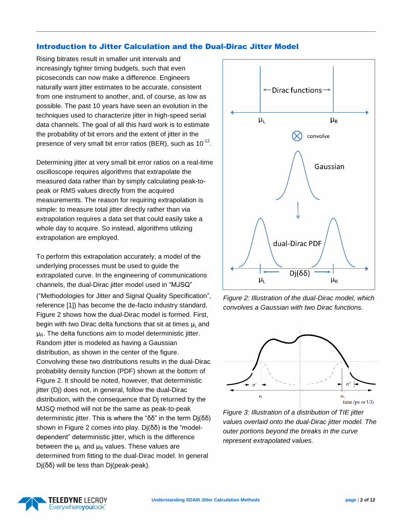
Figure 2 shows how the dual-Dirac model is formed. First,
begin with two Dirac delta functions that sit at times μL and
μR. The delta functions aim to model deterministic jitter.
Random jitter is modeled as having a Gaussian
distribution, as shown in the center of the figure.
Convolving these two distributions results in the dual-Dirac
probability density function (PDF) shown at the bottom of
Figure 2. It should be noted, however, that deterministic
jitter (Dj) does not, in general, follow the dual-Dirac
distribution, with the consequence that Dj returned by the
MJSQ method will not be the same as peak-to-peak
deterministic jitter. This is where the “δδ” in the term Dj(δδ)
shown in Figure 2 comes into play. Dj(δδ) is the “model-
dependent” deterministic jitter, which is the difference
between the μL and μR values. These values are
determined from fitting to the dual-Dirac model. In general
Dj(δδ) will be less than Dj(peak-peak).
Figure 2: Illustration of the dual-Dirac model, which
convolves a Gaussian with two Dirac functions.
Figure 3: Illustration of a distribution of TIE jitter
values overlaid onto the dual-Dirac jitter model. The
outer portions beyond the breaks in the curve
represent extrapolated values.
Understanding SDAIII Jitter Calculation Methods page | 3 of 12
Figure 3 shows an example histogram of acquired jitter measurements, along with the dual-Dirac Gaussians. The
tails of the histogram beyond the breaks in the curve show an extrapolation of the histogram. Determining these
extrapolated tails and the positions of μL and μR is the job of the algorithms discussed below, and requires a
determination of the sigma value used for the dual-Dirac Gaussians. In typical MJSQ implementations, the
assumption is made that σ- = σ+. The LeCroy NQ-Scale method does not make this assumption.
In MJSQ, total jitter (Tj) is the sum of deterministic jitter (Dj) and random jitter (Rj), with Rj weighted by a multiplier
α (alpha) that is determined from the bit error ratio. (α = 14.07 for a typical BER value of 10-12
):
Tj = α(BER)*Rj + Dj(δδ) (1)
Lastly, it is important to remember that model-based results are estimates, as opposed to directly measured
results like a straight-forward RMS or peak-to-peak value. Total jitter is essentially an estimate of the peak-to-
peak jitter at a specific bit error ratio.
Jitter Hierarchy
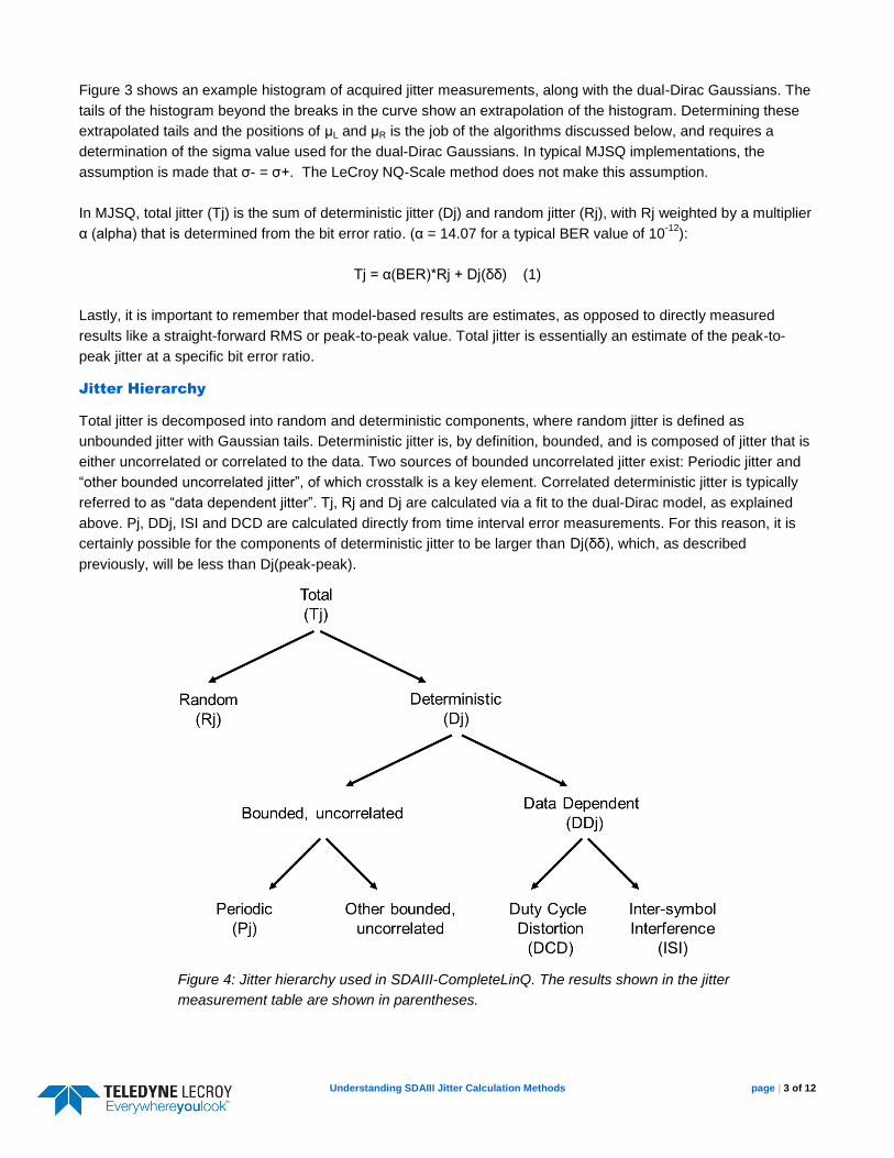
Total jitter is decomposed into random and deterministic components, where random jitter is defined as
unbounded jitter with Gaussian tails. Deterministic jitter is, by definition, bounded, and is composed of jitter that is
either uncorrelated or correlated to the data. Two sources of bounded uncorrelated jitter exist: Periodic jitter and
“other bounded uncorrelated jitter”, of which crosstalk is a key element. Correlated deterministic jitter is typically
referred to as “data dependent jitter”. Tj, Rj and Dj are calculated via a fit to the dual-Dirac model, as explained
above. Pj, DDj, ISI and DCD are calculated directly from time interval error measurements. For this reason, it is
certainly possible for the components of deterministic jitter to be larger than Dj(δδ), which, as described
previously, will be less than Dj(peak-peak).
Figure 4: Jitter hierarchy used in SDAIII-CompleteLinQ. The results shown in the jitter
measurement table are shown in parentheses.

Understanding SDAIII Jitter Calculation Methods page | 4 of 12
Overview of SDAIII Calculation Methods for Tj, Rj and Dj
SDAIII includes three methods to calculate Tj, Rj and Dj. All three methods are based on the dual-Dirac model,
but with different implementations. Users select which method to use via the Jitter Parameters dialog, and can
easily change from one method to another to compare the methods’ results. Here are short descriptions of each
method; additional information is provided later in the document.
Dual-Dirac Spectral Rj Direct Method:
The standard dual-Dirac model is used, with the σ (sigma) value of the Gaussians being derived from a spectral
analysis of the jitter. The tails of the jitter distribution are extrapolated using σ, but the final value for Rj is set to be
equal to σ. Tj is the width of the final cumulative distribution function (CDF) at the user’s selected BER level.
Dual-Dirac Spectral RJ+Dj CDF Fit:
As with the dual-Dirac Spectral Rj Direct method, the standard dual-Dirac model is used, with the σ (sigma) value
of the Gaussians being derived from a spectral analysis of the jitter. However, the tails of the jitter distribution are
extrapolated using σ with Tj equal to the width of the final cumulative distribution function (CDF) at the user’s
selected BER level, and Rj and Dj determined by fitting to equation (1) in the vicinity of the selected BER value.
This method most closely follows MJSQ, and is the default selection.
Dual-Dirac NQ-Scale:
“NQ-Scale” stands for “Normalized Q-Scale”. This is a variant of the dual-Dirac model that includes six degrees of
freedom: the Gaussians can have different σ (sigma) values, populations and means. The NQ-Scale method is
performed by transforming to the “Q-scale”, in which a Gaussian has a linear slope. Tj is the width of the final
cumulative distribution function (CDF) at the user’s selected BER level, and Rj and Dj are determined by fitting to
equation (1) in the vicinity of the selected BER value. Since the NQ-Scale method does not use spectral methods
to determine σ, and since it includes additional degrees of freedom, the estimates of jitter in the presence of high
crosstalk or other bounded, uncorrelated jitter may be more realistic than returned by the spectral methods.
Understanding SDAIII Jitter Calculation Methods page | 5 of 12
Jitter Calculation Methodology, Step-by-Step
Although this paper includes many details about how the jitter calculation is performed, it is not a “how-to” guide
for setting up the oscilloscope to make a measurement. Instead, this document aims to provide a high-level
description of how the oscilloscope calculates and decomposes jitter into Tj, Rj and Dj, and then further calculates
deterministic jitter components. See the LeCroy website for a thirty-minute tutorial, Jitter Basics Lab Using
SDAIII & Jitter Sim, along with the oscilloscope online help for information on setting up your oscilloscope.
Analysis Starting Point
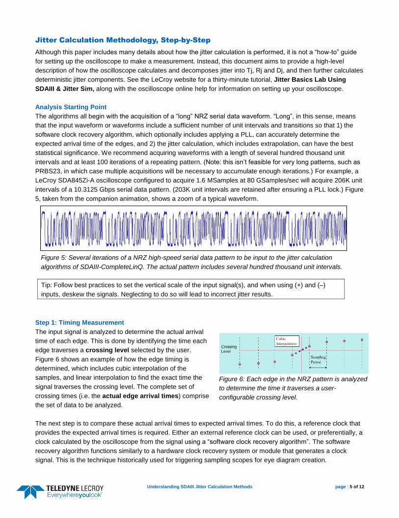
The algorithms all begin with the acquisition of a “long” NRZ serial data waveform. “Long”, in this sense, means
that the input waveform or waveforms include a sufficient number of unit intervals and transitions so that 1) the
software clock recovery algorithm, which optionally includes applying a PLL, can accurately determine the
expected arrival time of the edges, and 2) the jitter calculation, which includes extrapolation, can have the best
statistical significance. We recommend acquiring waveforms with a length of several hundred thousand unit
intervals and at least 100 iterations of a repeating pattern. (Note: this isn’t feasible for very long patterns, such as
PRBS23, in which case multiple acquisitions will be necessary to accumulate enough iterations.) For example, a
LeCroy SDA845Zi-A oscilloscope configured to acquire 1.6 MSamples at 80 GSamples/sec will acquire 206K unit
intervals of a 10.3125 Gbps serial data pattern. (203K unit intervals are retained after ensuring a PLL lock.) Figure
5, taken from the companion animation, shows a zoom of a typical waveform.
Tip: Follow best practices to set the vertical scale of the input signal(s), and when using (+) and (–)
inputs, deskew the signals. Neglecting to do so will lead to incorrect jitter results.
Step 1: Timing Measurement
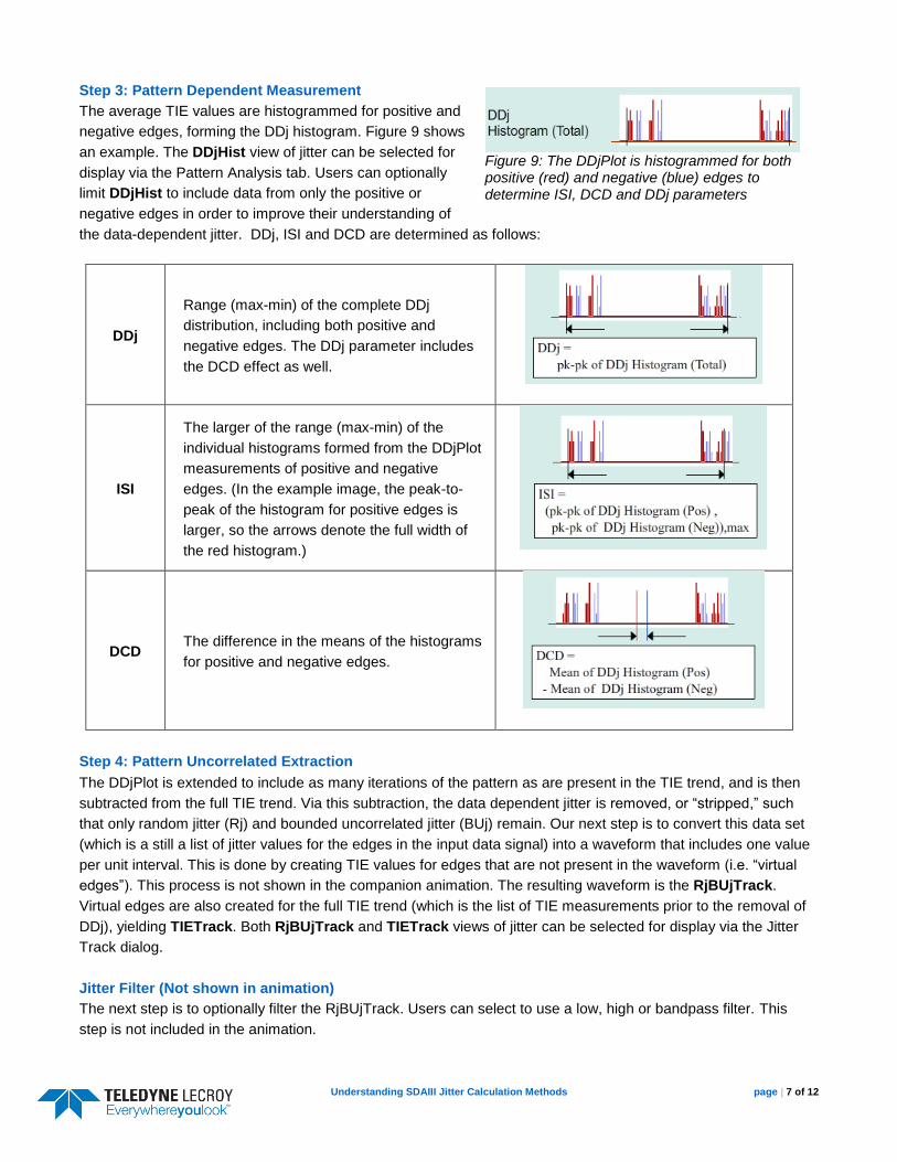
The input signal is analyzed to determine the actual arrival
time of each edge. This is done by identifying the time each
edge traverses a crossing level selected by the user.
Figure 6 shows an example of how the edge timing is
determined, which includes cubic interpolation of the
samples, and linear interpolation to find the exact time the
signal traverses the crossing level. The complete set of
crossing times (i.e. the actual edge arrival times) comprise
the set of data to be analyzed.
The next step is to compare these actual arrival times to expected arrival times. To do this, a reference clock that
provides the expected arrival times is required. Either an external reference clock can be used, or preferentially, a
clock calculated by the oscilloscope from the signal using a “software clock recovery algorithm”. The software
recovery algorithm functions similarly to a hardware clock recovery system or module that generates a clock
signal. This is the technique historically used for triggering sampling scopes for eye diagram creation.
Figure 5: Several iterations of a NRZ high-speed serial data pattern to be input to the jitter calculation
algorithms of SDAIII-CompleteLinQ. The actual pattern includes several hundred thousand unit intervals.
Figure 6: Each edge in the NRZ pattern is analyzed
to determine the time it traverses a user-
configurable crossing level.

Understanding SDAIII Jitter Calculation Methods page | 6 of 12
When recovering the clock from the data, the arrival times of the edges are input to a software clock recovery
algorithm that determines the underlying clock (and therefore the bitrate) of the input data stream. This algorithm
optionally applies a PLL that allows the oscilloscope to simulate the behavior of a receiver. Users can select from
a set of PLLs specific to a variety of serial data standards, or apply custom values. The output of this step is a
clock signal, as shown in Figure 7. The time of the clock edge closest to a specific data edge is the expected
arrival time for that data edge.
Once the clock arrival times are known, the expected arrival times
are subtracted from the actual arrival times to output a list of time
interval error (TIE) measurements. When viewed as a waveform,
this is the initial “TIE track”. (Note: At this point in the algorithm, the
TIE measurements are a list of values that are usually referred to as
a “trend” rather than a “track”. The animation does not make this
distinction. Also, the “TIE Trend” is not shown on the oscilloscope.)
Figure 7 shows TIE measurements for 5 example edges. One
negative TIE value is shown (edge #1), indicating an edge arriving
early; the other four are positive, indicating a late arrival.
The TIE values are direct measurements of jitter, and the
distribution of TIE measurements is used to determine total, random and deterministic jitter after extrapolating
the tails of the distribution in order to estimate jitter at low BER levels.
Step 2: Pattern Dependent Extraction
The first step in characterizing data-dependent jitter
(including intersymbol interference and duty cycle
distortion) is to look for a repeating pattern in the
signal. When no repeating pattern is present, a non-
repeating method can be used to look for repetition
of bit sequences of a user-defined length. (The non-
repeating method is not described in this paper.)
Once the repeating pattern is found, the TIE
measurements are analyzed to determine an
average TIE value for each bit in the repeating
pattern. Figure 8 shows this analysis. Corresponding
TIE measurements of each iteration of the pattern
are averaged resulting in a waveform that contains
only data-dependent jitter.
This results in an “average TIE trend” waveform,
called the DDjPlot. Figure 8 shows this process. The digital pattern found (DigPatt) and the DDjPlot views of
jitter can be selected for display from the Pattern Analysis dialog.
Figure 7: Illustration showing arrival times
of several edges and the recovered clock.
Time interval error (TIE) measurements
are the difference between actual and
expected arrival times.
Figure 8: The process of determining data-dependent jitter
begins with finding the average TIE value for each edge in
the pattern. The result is the DDjPlot.
Understanding SDAIII Jitter Calculation Methods page | 7 of 12
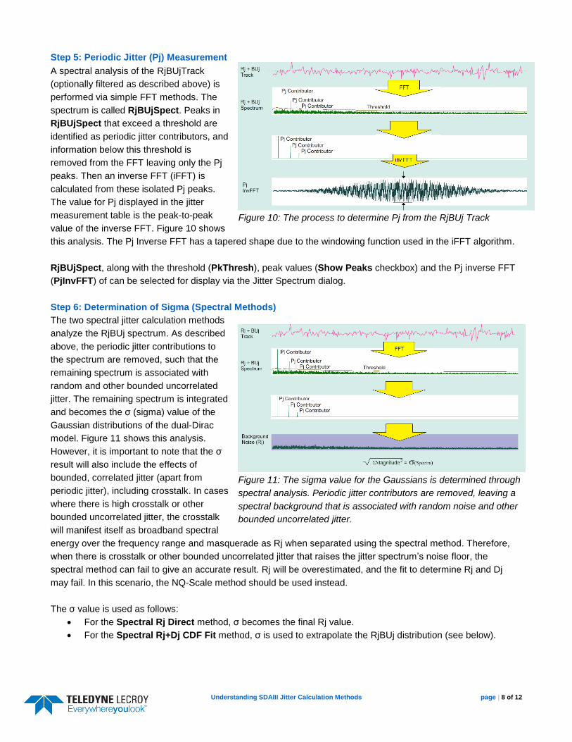
Step 3: Pattern Dependent Measurement
The average TIE values are histogrammed for positive and
negative edges, forming the DDj histogram. Figure 9 shows
an example. The DDjHist view of jitter can be selected for
display via the Pattern Analysis tab. Users can optionally
limit DDjHist to include data from only the positive or
negative edges in order to improve their understanding of
the data-dependent jitter. DDj, ISI and DCD are determined as follows:
DDj
Range (max-min) of the complete DDj
distribution, including both positive and
negative edges. The DDj parameter includes
the DCD effect as well.
ISI
The larger of the range (max-min) of the
individual histograms formed from the DDjPlot
measurements of positive and negative
edges. (In the example image, the peak-to-
peak of the histogram for positive edges is
larger, so the arrows denote the full width of
the red histogram.)
DCD The difference in the means of the histograms
for positive and negative edges.
Step 4: Pattern Uncorrelated Extraction
The DDjPlot is extended to include as many iterations of the pattern as are present in the TIE trend, and is then
subtracted from the full TIE trend. Via this subtraction, the data dependent jitter is removed, or “stripped,” such
that only random jitter (Rj) and bounded uncorrelated jitter (BUj) remain. Our next step is to convert this data set
(which is a still a list of jitter values for the edges in the input data signal) into a waveform that includes one value
per unit interval. This is done by creating TIE values for edges that are not present in the waveform (i.e. “virtual
edges”). This process is not shown in the companion animation. The resulting waveform is the RjBUjTrack.
Virtual edges are also created for the full TIE trend (which is the list of TIE measurements prior to the removal of
DDj), yielding TIETrack. Both RjBUjTrack and TIETrack views of jitter can be selected for display via the Jitter
Track dialog.
Jitter Filter (Not shown in animation)
The next step is to optionally filter the RjBUjTrack. Users can select to use a low, high or bandpass filter. This
step is not included in the animation.
Figure 9: The DDjPlot is histogrammed for both positive (red) and negative (blue) edges to determine ISI, DCD and DDj parameters
Understanding SDAIII Jitter Calculation Methods page | 8 of 12
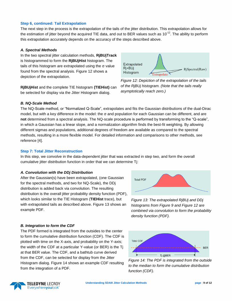
Step 5: Periodic Jitter (Pj) Measurement
A spectral analysis of the RjBUjTrack
(optionally filtered as described above) is
performed via simple FFT methods. The
spectrum is called RjBUjSpect. Peaks in
RjBUjSpect that exceed a threshold are
identified as periodic jitter contributors, and
information below this threshold is
removed from the FFT leaving only the Pj
peaks. Then an inverse FFT (iFFT) is
calculated from these isolated Pj peaks.
The value for Pj displayed in the jitter
measurement table is the peak-to-peak
value of the inverse FFT. Figure 10 shows
this analysis. The Pj Inverse FFT has a tapered shape due to the windowing function used in the iFFT algorithm.
RjBUjSpect, along with the threshold (PkThresh), peak values (Show Peaks checkbox) and the Pj inverse FFT
(PjInvFFT) of can be selected for display via the Jitter Spectrum dialog.
Step 6: Determination of Sigma (Spectral Methods)
The two spectral jitter calculation methods
analyze the RjBUj spectrum. As described
above, the periodic jitter contributions to
the spectrum are removed, such that the
remaining spectrum is associated with
random and other bounded uncorrelated
jitter. The remaining spectrum is integrated
and becomes the σ (sigma) value of the
Gaussian distributions of the dual-Dirac
model. Figure 11 shows this analysis.
However, it is important to note that the σ
result will also include the effects of
bounded, correlated jitter (apart from
periodic jitter), including crosstalk. In cases
where there is high crosstalk or other
bounded uncorrelated jitter, the crosstalk
will manifest itself as broadband spectral
energy over the frequency range and masquerade as Rj when separated using the spectral method. Therefore,
when there is crosstalk or other bounded uncorrelated jitter that raises the jitter spectrum’s noise floor, the
spectral method can fail to give an accurate result. Rj will be overestimated, and the fit to determine Rj and Dj
may fail. In this scenario, the NQ-Scale method should be used instead.
The σ value is used as follows:
For the Spectral Rj Direct method, σ becomes the final Rj value.
For the Spectral Rj+Dj CDF Fit method, σ is used to extrapolate the RjBUj distribution (see below).
Figure 10: The process to determine Pj from the RjBUj Track
Figure 11: The sigma value for the Gaussians is determined through
spectral analysis. Periodic jitter contributors are removed, leaving a
spectral background that is associated with random noise and other
bounded uncorrelated jitter.
Understanding SDAIII Jitter Calculation Methods page | 9 of 12
Step 6, continued: Tail Extrapolation
The next step in the process is the extrapolation of the tails of the jitter distribution. This extrapolation allows for
the estimation of jitter beyond the acquired TIE data, and out to BER values such as 10-12
. The ability to perform
this extrapolation accurately depends on the accuracy of the steps described above.
A. Spectral Methods
In the two spectral jitter calculation methods, RjBUjTrack
is histogrammed to form the RjBUjHist histogram. The
tails of this histogram are extrapolated using the σ value
found from the spectral analysis. Figure 12 shows a
depiction of the extrapolation.
RjBUjHist and the complete TIE histogram (TIEHist) can
be selected for display via the Jitter Histogram dialog.
B. NQ-Scale Method
The NQ-Scale method, or “Normalized Q-Scale”, extrapolates and fits the Gaussian distributions of the dual-Dirac
model, but with a key difference in the model: the σ and population for each Gaussian can be different, and are
not determined from a spectral analysis. The NQ-scale procedure is performed by transforming to the “Q-scale”,
in which a Gaussian has a linear slope, and a normalization algorithm finds the best-fit weighting. By allowing
different sigmas and populations, additional degrees of freedom are available as compared to the spectral
methods, resulting in a more flexible model. For detailed information and comparisons to other methods, see
reference [4].
Step 7: Total Jitter Reconstruction
In this step, we convolve in the data-dependent jitter that was extracted in step two, and form the overall
cumulative jitter distribution function in order that we can determine Tj:
A. Convolution with the DDj Distribution
After the Gaussian(s) have been extrapolated, (one Gaussian
for the spectral methods, and two for NQ-Scale), the DDj
distribution is added back via convolution. The resulting
distribution is the overall jitter probability density function (PDF),
which looks similar to the TIE Histogram (TIEHist trace), but
with extrapolated tails as described above. Figure 13 shows an
example PDF.
B. Integration to form the CDF
The PDF formed is integrated from the outsides to the center
to form the cumulative distribution function (CDF). The CDF is
plotted with time on the X-axis, and probability on the Y-axis;
the width of the CDF at a particular Y-value (or BER) is the Tj
at that BER value. The CDF, and a bathtub curve derived
from the CDF, can be selected for display from the Jitter
Histogram dialog. Figure 14 shows an example CDF resulting
from the integration of a PDF.
Figure 12: Depiction of the extrapolation of the tails
of the RjBUj histogram. (Note that the tails really
asymptotically reach zero.)
Figure 13: The extrapolated RjBUj and DDj
histograms from Figure 9 and Figure 12 are
combined via convolution to form the probability
density function (PDF).
Figure 14: The PDF is integrated from the outside
to the median to form the cumulative distribution
function (CDF).

Understanding SDAIII Jitter Calculation Methods page | 10 of 12
Step 8: Tj, Rj, Dj Calculation
Tj Determination
For all methods, Tj is the width of the CDF at the user’s selection for BER. Note that the CDF for NQ-scale is
determined differently than the two spectral methods.
Rj and Dj Determination:
(Spectral Rj+Dj CDF Fit Method)
To determine Rj and Dj when using the Rj+Dj CDF Fit
method, the CDF is fitted to the Dual Dirac model
equation Tj = α(BER)*Rj + Dj(δδ), where α(BER) is the
confidence interval at a confidence level of 1-BER for a
single “normal” Gaussian. (For example, α ~= 14.07 for
BER = 10-12
). The points on the CDF that are used in
the fit include the selected BER, 1 point above, and two
below. For example, for a selected BER of 10-12
, the CDF points used for the fit are BER=10-11
, 10-12
, 10-13
and 10-14
.) See Figure 15.
Rj and Dj (Spectral Rj Direct Method)
In the Spectral Rj Direct method, Rj is determined directly from the jitter spectrum. Dj is then determined by
fitting the CDF with the constraint that Rj = σ. Deriving Rj directly from the spectrum rather than via a fit typically
produces lower values of Rj. Limitations of this method are discussed below in the section “Variation of Rj with
Pattern Length”.
Rj and Dj Determination: (NQ-scale Method)
In the NQ-Scale method, Rj and Dj are determined from the CDF using the same technique as for Rj+Dj CDF Fit,
but since the CDF for NQ-scale is determined much differently than for the two spectral methods, the Rj and Dj
results will be different. See Step 6B above for more information regarding the CDF calculation for the NQ-Scale
method.
Variation of Rj with Pattern Length
This Spectral Rj Direct method typically gives the lowest value of Rj, but at the expense of deviating from the
MJSQ jitter calculation methodology, which specifies that Rj and Dj should be derived by fitting to a dual-Dirac
jitter model. This method is included in SDAIII to provide a result that closely correlates to jitter calculation
methodologies on sampling oscilloscopes that cannot perform Rj and Dj separation using a repeating pattern
technique. For a channel that includes even a small amount of intersymbol interference (ISI), a fit to the dual-
Dirac jitter model as described in MJSQ should result in Rj that increases with pattern length. This is due to the
fact that as pattern lengths grow, the data-dependent jitter (DDj) distribution increasingly takes on a Gaussian
shape with growing tails. These tails cause the fit to the equation Tj = α(BER)*Rj + Dj(δδ) to return an Rj value
that increases with pattern length. Note that bit error rate testers (BERT) will also return increasing Rj with pattern
length. When using Spectral Rj Direct, Rj will not show grow with pattern length, since it is determined directly
from the jitter spectrum and not via a fit.
Figure 15: In the Spectral Rj+Dj CDF Fit and NQ-Scale
methods, Rj and Dj are determined by fitting to
Tj(BER) = α(BER)*Rj + Dj

Understanding SDAIII Jitter Calculation Methods page | 11 of 12
Last Step: Display results
Users can display the jitter measurements in the
SDA jitter table, as show in Figure 16. Notice that
the table includes a header row: the Tj column
header indicates the BER value selected by the
user, and the Rj and Dj header indicates which
method is in use. For Rj direct: “spD”; for Rj+Dj CDF Fit: “sp”; for NQ-Scale: “nq”.
When using the SDAIII products that include the ability to simultaneously measure jitter on up to four lanes
simultaneously (“LinQ” is part of the part number for these products), the views of jitter are shown within a
“LaneScape” for each lane. Up to 40 traces can be displayed simultaneously, arranged in a large variety of user-
selectable grid modes, with 1, 2 or all lanes displayed at a time. Figure 17 shows a comparison of two lanes in
dual LaneScape mode, showing many of the views of jitter discussed in this document.
Figure 16: Table showing the jitter measurement results. The
column header indicates which method is employed. (In this
case, it indicates "sp", which is Rj+Dj CDF Fit.
Figure 17: Screenshot showing SDA analysis on four lanes, showing the jitter table along with a wide variety of views.

Understanding SDAIII Jitter Calculation Methods page | 12 of 12
Conclusions
The SDAIII-CompleteLinQ calculates jitter on long serial data waveforms using one of several dual-Dirac based
models, and finds components of data-dependent jitter directly from TIE measurements. Users can choose to
display a wide range of jitter results, including summary results, such as Tj, Rj, Dj, DDj, ISI, DCD and Pj, as well
as views that provide insight into the sources of jitter quantified in the results listed above. Views include spectra,
histograms and jitter tracks that describe jitter in the time, frequency and statistical domains. Users are
encouraged to examine the jitter tracks, spectra and histograms in order to understand the nature of jitter
aggressors and to determine which method to use for determining final jitter values. Three methods for calculating
Tj and decomposition into Rj and Dj have been described, including two spectral methods and LeCroy’s NQ-scale
method. When crosstalk or other bounded-uncorrelated jitter is present, the NQ-Scale method will give the most
realistic jitter estimates.
Questions, comments or suggestions regarding this document are welcomed, and can be emailed to
Additional Reading
[1] “Fibre Channel - Methodologies for Jitter and Signal Quality Specification- MJSQ”. T11, 5 June, 2005.
http://www.t11.org (t11.org membership required.)
[2] Miller, Marty and Schnecker, Michael. “A Comparison of Methods for Estimating Total Jitter Concerning
Precision, Accuracy and Robustness.” DesignCon2007.
<http://cdn.lecroy.com/files/whitepapers/lecroy_jitter_methods_designcon2007.pdf>
[3] Miller, Marty. “6 Tales of Rj and Dj.” LeCroy Corporation Website, 2005.
<http://cdn.lecroy.com/files/whitepapers/wp_techbrief_rj_and_dj.pdf >
[4] Miller, Marty. “Normalized Q-scale Analysis: Theory and Background.” EDN Magazine. 16 March, 2007.
<http://www.edn.com/design/test-and-measurement/4314553/Normalized-Q-scale-analysis-Theory-and-
background>
[5] Miller, Marty and Schnecker, Michael. “Quantifying Crosstalk Induced Jitter in Multi-lane Serial Data Systems.”
DesignCon2009. <http://cdn.lecroy.com/files/whitepapers/lecroy_jitter_methods_designcon2007.pdf>