Uncertainty propagation in model chains: a case...

Uncertainty propagation in model chains: a case study in natureconservancy

E.P.A.G. SchouwenbergH. HouwelingM.J.W. JansenJ. KrosJ.P. Mol-Dijkstra

Alterra-rapport 001

Alterra, Green World Research, Wageningen, 2000

Alterra-rapport 001 2

ABSTRACT

Schouwenberg, E.P.A.G., H. Houweling, M.J.W. Jansen, J.Kros and J.P. Mol-Dijkstra, 2000.Uncertainty propagation in model chains: a case study in nature conservancy. Wageningen, Alterra, GreenWorld Research. Alterra-rapport 001. 90 p.; 14 fig.; 9 tab.; 36 ref.; 3 annexes

The availability of high-quality models is considered as a critical success factor for Alterra. Toanswer the complex questions of policy makers it is often necessary to link models that havebeen developed initially to study more limited questions. When models are linked errorpropagation may enlarge the uncertainty of the model results. However the quantification ofuncertainty propagation may become more complex. This problem of uncertainty propagation inmodel chains is explored using a chain of the models SMART2/SUMO, P2E and NTM thatpredicts the potential nature conservation value of natural areas.Two methods have been explored to study the uncertainty propagation in the model chain, aregression-free method that estimates the uncertainty contributions of groups of sources ofuncertainty, and an analysis by means of linear regression approximations of the sub-models ofthe model chain. The final analysis was done with a regression-free method. The results arepresented as the contributions of the various sources of uncertainty to the uncertainty of thepotential conservation value. From the results of this study, lessons are learned for the analysesof error propagation in model chains.

Keywords: model chains, NTM, SMART2/SUMO, SMART2, SUMO, uncertainty analysis,uncertainty propagation, WINDINGS

ISSN 1566-7197

This report can be ordered by paying 51,25 Dutch guilders into bank account number36 70 54 612 in the name of Alterra, Wageningen, the Netherlands, with reference to Alterra-rapport 001. This amount is inclusive of VAT and postage.

© 2000 Alterra, Green World Research,P.O. Box 47, NL-6700 AA Wageningen (The Netherlands).Phone: +31 317 474700; fax: +31 317 419000; e-mail: [email protected]

No part of this publication may be reproduced or published in any form or by any means, or stored in adata base or retrieval system, without the written permission of Alterra.

Alterra assumes no liability for any losses resulting from the use of this document.

Alterra is the amalgamation of the Institute for Forestry and Nature Research (IBN) and the WinandStaring Centre for Integrated Land, Soil and Water Research (SC). The merger took place on 1 January2000.

Project 636-35374-01 [Alterra-rapport 001/HM/05-2000]

Contents

Preface 7

Summary 9

1 Introduction 13

2 The case study: model chain and experimental design 172.1 The case study 172.2 Description of the model chain 17

2.2.1 SMART2/SUMO 182.2.2 NTM 192.2.3 Conversion model P2E 21

2.3 Experimental design 22

3 Inventory of sources of uncertainty 253.1 Sources of error 253.2 Grouping of sources of error reflecting chain character 273.3 Overview of inspected parameters and unexplained system variation 283.4 Specification of errors in parameter values 28

3.4.1 SMART2/SUMO 283.4.2 P2E 283.4.3 NTM 33

4 Methods 354.1 Variance-based uncertainty contributions of groups of inputs 364.2 Estimation of uncertainty contributions of independent pooled sources 374.3 Chain analysis via linear approximations of i/o relations of sub-models 39

5 Results of the case study 415.1 Overview of the performed analysis 415.2 Uncontrolled succession from bare ground 42

5.2.1 Analysis without USV 425.2.2 Analysis with USV 46

5.3 Succession of current vegetation 505.3.1 Analysis without USV 505.3.2 Analysis with USV 51

5.4 Summary 52

6 Conclusions 556.1 Uncertainty propagation in the model chain SMART/SUMO-P2E-NTM 556.2 Lessons learned for analyses of error propagation in model chains 566.3 Recommendations for development and uncertainty analysis of model

chains 57

References 59


Annexes

1 List of symbols 632 Estimation of uncertainties in P2E and NTM 653 Results of the WINDINGS analysis 73


Preface

This project has been carried out within the framework of the program for StrategicKnowledge Development of Alterra, in close co-operation with the Centre forBiometry of Plant Research International. It is one of the projects supervised byVEMI, the Alterra platform that has been established to raise the quality of themodels and data used by Alterra .


Summary

The availability of high-quality models is considered as a critical success factor forAlterra. Several models of Alterra are essential tools in the projects for the DutchNature Policy Assessment Office (NPB) and the Environmental Policy AssessmentOffice (MPB). Knowledge of the reliability of the model results is a precondition forthe application of these models. To answer the complex questions of policy makers,it is often necessary to link models that have been developed initially to study morelimited questions. When models are linked, error propagation may enlarge theuncertainty of the model results and the complexity of the chain with severalcomponents and feedback's makes an uncertainty analysis more complicated. To gaininsight in this problem of uncertainty propagation we approached the issue from thefollowing research questions:- how can uncertainty propagation in model chains be analysed?- how is model input uncertainty translated into model output uncertainty in a real

model chain?- which general recommendations can be made for uncertainty analysis in model

chains?

The problem was studied using a model-chain, consisting of the models SMART2,SUMO and NTM. SMART2 and SUMO are fully integrated already.SMART2/SUMO describes nutrient cycling in terrestrial (semi)natural ecosystemsand predicts the biomass growth and vegetation succession. Input data forSMART2/SUMO are a deposition scenario and data about soil, hydrology, andvegetation structure and vegetation management. NTM is a model for the predictionof the potential nature conservation value (PCV) of natural areas. SMART2/SUMOis linked to NTM by a module called P2E, that converts mean spring groundwaterlevel and the output of SMART2/SUMO, pH and N availability, into the input forNTM, which means Ellenberg indication values.

To examine the problem of uncertainty propagation in model-chains within a limitedperiod of time, we simplified the problem considerably. Although the model-chainSMART2/SUMO-P2E-NTM is generally used to generate regional or nation-wideimages, we only studied a limited number of local spots. Errors in spatial informationlike soil map and vegetation map were not investigated. Uncertainty in depositionand hydrological scenarios was not considered. The analysis included errors arisingfrom uncertainty about parameter values, given the soil type and the initial vegetationtype. Moreover, the analysis included errors in the structure of the sub-models P2Eand NTM that showed up during the estimation of the parameters of these sub-models using field measurements. It appeared, not amazingly, that the inputs of thesesub-models are not the only factors that influence the output variables in the field:when the inputs are identical, the measurements of the field systems varies more thancan be explained by measurement errors. This variation was called ‘unexplainedsystem variation’. For SMART2/SUMO, of which the parameters were estimatedpreviously, only parameter uncertainty was taken into account. In total, 36 individual


sources of error were analysed. Error propagation contributions through the model-chain, was estimated for the following six groups of uncertainty sources having adistinct place in the chain:- soil related parameters (SMART2/SUMO);- vegetation-related parameters (SMART2/SUMO);- P2E parameters;- NTM parameters;- unexplained system variation P2E;- unexplained system variation NTM.

For each group, the contribution to the uncertainty of the potential conservationvalue (PCV) was estimated.

Two methods have been explored to study the uncertainty propagation in the modelchain, a regression-free method that estimates the uncertainty contributions of theabove-mentioned six groups of sources of uncertainty, and an analysis by means oflinear regression approximations of the three submodels of the model chain.The final analysis was done with the regression-free method. The analysis was donewith and without accounting for unexplained system variation of P2E and NTM.The uncertainty in the model results is most relevant for policy making when twoscenarios are compared.

Two policy scenarios and two vegetation management scenarios were considered.An analysis was done for the policy scenario “business as usual” that supposesunchanged policy concerning deposition, a second analysis was done to compare thescenarios “business as usual” and “European co-ordination” which supposes adecreasing input of potential acid. The analysis was done for uncontrolled successionfrom bare ground for three soil types and a succession from the current vegetationfor one soil type.

The results of the uncertainty analysis of this specific sequence of models arepresented as the contributions of the various sources to the uncertainty of thepotential conservation value (PCV). When inspecting the difference between the twoscenarios, the analysis ends in the following results:- When the unexplained system variation of P2E and NTM is not taken into

account, the SMART2/SUMO vegetation parameters make the largestcontribution to the uncertainty of PCV at both succession stages (successionfrom bare ground and succession of current vegetation). At succession of thecurrent vegetation, the NTM parameters also contribute noticeably to theuncertainty of PCV (fig. 8, 12).

- When we take into account the unexplained system variation of P2E and NTM,the USV of P2E also contributes much to the uncertainty of PCV. Thiscontribution decreases in the long run (fig. 10, 14).

- There is little influence of the soil type in the case of succession from bareground. We did not examine the influence of soil type in the case of successionof current vegetation.


When the absolute potential conservation value is examined rather than thedifference between to scenarios, the contribution of the unexplained system variationof NTM to the uncertainty of PCV is important (fig. 9, 13). When the unexplainedsystem variation is left out of consideration the vegetation-related parameters ofSMART2/SUMO, the P2E parameters and NTM parameters contribute most to theuncertainty of PCV. The results also illustrate the more general phenomenon thatabsolute predictions tend to be less accurate than relative predictions. The varianceof the difference between the predicted conservancy values of two scenarios hadmuch smaller values than the variance of the individual predicted conservancy values.Some sources of uncertainty, like unexplained system variation, more or less cancelout when differences are analysed. This is a fortunate circumstance, since differencesbetween scenarios are more relevant for decision making.

We conclude that in this specific case only at managed vegetation development theuncertainty analysis makes sense. At unmanaged vegetation development from bareground, the vegetation structure and the related nutrient catchment change soradically that the difference due to the two atmospheric deposition scenarios isnegligible.

Lessons learned for the analyses of error propagation in model chains are:- For the analysis of the error propagation in a model-chain like the slightly

simplified one studied in this project, the required knowledge and tools areavailable.

- The main problem is the limited information about the uncertainty of therelevant input data and model parameters. A second problem is the limitedpossibilities to gain insight in the unexplained system variation in models likeSMART2/SUMO.

- In general, the uncertainty analysis asks a substantial effort, even when importantaspects like the uncertainty in soil- and vegetation maps are left aside. The mostlabour-intensive and time-consuming activities are data collection aboutuncertainty of model inputs and parameters. However, the results of this lattereffort can be used in new applications of the model-chain.

- Uncertainty propagation in vegetation and conservation value modelling creates anew need for data. There is a considerable backlog on quantification ofuncertainty of model inputs and on documentation of parameterisation.

- With regard to uncertainty analysis, model chains are not different from any kindof complex models arising by combining existing sub-models. However onlyscientific problems are considered here, there may be serious managementproblems when sub-models and data come from different organisations.


1 Introduction

The interest of AlterraSimulation models play an important role in the research at Alterra. The quality ofthese models is considered as a critical success factor. Several models of Alterra areessential tools in the analyses by the Dutch Nature Policy Assessment Office (NPB)and the Environmental Policy Assessment Office (MPB). To answer complexquestions of policy makers models are linked that initially have been developed tostudy more limited questions. When models are linked some additional problemsarise. Error propagation enlarges the uncertainty of the model results and thecomplexity of the chain with several components and feedback's makes theuncertainty analysis more complicated. Therefore, in the framework of the Alterraprogramme for Strategic Knowledge Development (Dutch: Strategische ExperiseOntwikkeling, SEO), a pilot project has been carried out to gain insight in errorpropagation and uncertainty aspects of model chains.

The research questions are:- how can uncertainty propagation in model chains be analysed?- how is model input uncertainty translated in model output uncertainty in a real

model chain?- Which general recommendations can be made for uncertainty analysis of model

chains?

A simple chain of modelsIn this project uncertainty propagation was studied in a chain of models that is notextremely complicated at first sight. This chain consists of the models SMART2(Kros et al. 1995), SUMO (Wamelink et al. 2000) and NTM (Wamelink 1997,Schouwenberg in prep.). SMART2 describes nutrient cycling and soil acidification interrestrial (semi)natural ecosystems. SUMO models biomass growth and vegetationsuccession and NTM predicts the potential nature conservation value of semi naturalecosystems. SMART2 and SUMO have been fully integrated into one modelSMART2/SUMO. SMART2/SUMO is linked to NTM by a conversion modulecalled P2E, that converts mean spring groundwater level and the output ofSMART2/SUMO, pH and N availability, into suitable input for NTM, Ellenbergindication values. An interesting aspect of the use of the SMART2/SUMO-P2E-NTM chain in this project is the nature of the models that comprise this chain.SMART2/SUMO is a process model, built up from the mathematical description ofphysical, chemical and biological processes whereas NTM is a descriptive model thatrelates measurements of abiotic variables to the conservation value of the spot. Theyrepresent two important model types that are developed and used by Alterra.Although the model chain SMART2/SUMO-P2E-NTM will play an important rolein the outlooks of NPB and MPB we just use it as an instrument to study the subjectof uncertainty propagation in model chains. The results of this project are evaluatedand generalised in such a way that they are useful for future analyses of other chainsof models.


UncertaintyUncertainty analysis translates model input uncertainty into model output uncertaintyand pinpoints the inputs that contribute most to output uncertainty. The analysisgives an impression of the accuracy of the predictions of the model study, andsuggests ways to improve the accuracy. There is an extensive experience with thesensitivity and uncertainty analysis of more or less complex models. The chains ofmodels studied here has the peculiarity that the need to link the models arose afterthe components SMART2, SUMO and NTM were developed as separate modelswith their own limited area of application. The conversion module P2E was neededto link SMART2/SUMO to NTM.

Uncertainty analysis of a model study begins with making up an inventory of thesources of error for the case at hand. In the type of uncertainty analysis discussedhere -- the most common one -- uncertainty in a source of error is modelled byconsidering these sources as random vectors, which are input to the model. Thespecification of the distributions of the sources of uncertainty is by far the mostdifficult stage of an uncertainty analysis. The last stage of the analysis translates theuncertainty in these sources into model output uncertainty (randomness) andpinpoints the inputs, or groups of inputs, that contribute most to output uncertainty.

There are several sources of uncertainty; the scenarios that have to be analysed, initialvalues, parameter values and the mathematical formulation and structure of themodel. To explore the problem of uncertainty propagation in model chains within alimited period, we have defined a simplified problem. Firstly errors in exogenousvariables like deposition and hydrological scenarios were not considered. Secondlythe model chain SMART2/SUMO-P2E-NTM is normally used to generate regionaland nation wide images but we did the analysis for a limited number of local spots.Errors in spatial information like soil map and vegetation map were left out ofconsideration and deposition and hydrological scenarios were taken for sure. Theanalysis was delimited to uncertainty originating from errors in parameter values andmodel structure. For SMART2/SUMO only parameter uncertainty was taken intoaccount. The analysis focussed on six groups of model-input data and parameters,covering 36 sources of uncertainty. For each group, the contribution to theuncertainty of the output of NTM (the potential conservation value PCV) wasestimated. The models are validated in the project 'Validation Natuurplanner'(Wamelink et al. 2000).

Outline of the reportChapter 2 describes the components of the chain of models: SMART2/SUMO,NTM and the module P2E that has been developed to convert the output of SUMOto input for NTM. In chapter 3 we present an overview of the sources of uncertaintyin the chain of models. In Chapter 4 the methods are discussed that were used in thisstudy. Two methods have been applied; a Monte Carlo type method, the regressionfree windings stairs analysis and a method where variance contributions are estimatedby means of linear approximations of the modules in the chain. In chapter 5 theresults are presented. The uncertainty propagation in the model chain is quantified.The uncertainty in the outcome for various scenarios, the uncertainty in the


comparison of scenarios and the relative contributions of the various sources ofuncertainty are presented. In the last chapter lessons learned and suggestions forfurther model development are given.


2 The case study: model chain and experimental design

2.1 The case study

In the case study uncertainty propagation is studied in the chain consisting of themodels SMART2/SUMO, P2E and NTM. An advantage of the use of theSMART2/SUMO-P2E-NTM chain in this project is the nature of the models thatcomprise this chain. SMART2 and SUMO are process orientated models, built upfrom the mathematical description of physical, chemical and biological processeswhile NTM and P2E are statistical models that relate the values of observedparameters to a judgement of the potential conservation value of the spot. Theyrepresent two important model types that are developed and used by Alterra.

2.2 Description of the model chain

The model chain consists of three models (figure 1). The first model is the soil-vegetationsuccession model SMART2/SUMO that calculates abiotical quantities andsuccession stages. The last model, NTM calculates the potential conservation valuefor the considered situation. A conversion model P2E that converts the abioticaloutput from SMART2/SUMO into Ellenberg indication values for NTM links bothmodels.

Sources of uncertainty in model chain SMART/SUMO/NTM

SMART2/SUMO(SMS)

P2E NTM

SMSS

Potentialconservation

value

e_R

e_N

e_F

pH

Nav

MSGL

SMSSV

SMSs Soiltype related SMS parameters

SMSv Vegetationtype related SMS parametersSMSsv Soil and vegetation related SMS parameters

RCp2e Regression coefficients of Phys2Ellen regression equations

RCntm Regression coefficients of NTM regression equations

USV Unexplained system variation

Model

Inspected modelparameters

Inspected Modelinputs /-outputs

Spatial variable modelinputs; uncertainty not inspected(deposition and hydrology are also temporal variable)

Ndep , Sdep

Soilmap

Vegetationmap

Deposition

Hydrology

SMS v

Not inspected Modelinputs /-outputs

USV USV

Inspected modelstructure aspects

RC p2e RC ntmVeg. type

Figure 1: The model chain SMART2/SUMO-P2E-NTM


Input data for the SMART2/SUMO application at a national scale can be dividedinto system input such as deposition and hydrology and initial values of variables andparameters. Input data refer to: (i) a specific deposition scenario for each gridcell, (ii)model variables and parameters that are either related to a soil type (SMS s) or to avegetation type (SMSv) or a combination of both (SMSsv), and (iii) soil and vegetationmaps. The mean spring groundwater level (MSGL) is derived from the groundwatertable class from the 1:50,000 soil map and is kept constant. Outputs of the modelSMART2/SUMO are the abiotic quantities pH, and N availability and the bioticquality vegetation type or succession stage.

The model P2E converts pH, N availability and MSGL to Ellenberg indicationvalues for respectively acid (e_R), nutrient availability (e_N) and moisture (e_F). Atthe end, NTM uses these Ellenberg indication values to predict a potentialconservation value (PCV) for each gridcell.

Uncertainties in parameters related to soil type (SMS s), parameters related tovegetation type (SMSv) and regression coefficients (RC) were considered.Occasionally, however, for instance during the parameterisation of a model, one mayidentify and quantify model errors of a type that will be called unexplained systemvariation (USV). This also appeared for P2E and NTM (see section 3.1). Theunexplained system variation of SMART2/SUMO was not known and was thereforeleft out of consideration. Parameters that were related to a combination of soil typeand vegetation type (SMS sv) did not occur; hence we did simulations per soil type(see section 2.3).

2.2.1 SMART2/SUMO

SMART2 (Kros et al. 1995) is a simple one-compartment soil acidification andnutrient cycling model that includes the major hydrological and biogeochemicalprocesses in the vegetation, litter and mineral soil. Apart from pH, the model alsopredicts changes in aluminium (Al3+), base cation (BC), nitrate (NO3

-) and sulphate(SO4

2-) concentrations in the soil solution and solid phase characteristics depictingthe acidification status, i.e. carbonate content, base saturation and readily available Alcontent. The SMART2 model consists of a set of mass balance equations, describingthe soil input-output relationships, and a set of equations describing the rate-limitedand equilibrium soil processes. The soil solution chemistry in SMART2 dependssolely on the net element input from the atmosphere and groundwater, canopyinteractions, geochemical interactions in the soil and a complete nutrient cycle forbasic cations and N. The description is based on the assumption that the amount oforganic matter (C) is proportional to nitrogen (N). N mineralisation is described inSMART2 by a first order reaction. Litterfall and growth of the vegetation aremodelled by the succession model SUMO (Wamelink et al. 2000), that wasincorporated in the model SMART2 in 1998 (figure 2). Depending on the amount ofavailable nitrogen (Nav) (2 in figure 2), SUMO calculates biomass growth, root uptakeand amount of litterfall (3 in figure 2). In the same time step (=year) SMART2calculates the mineralisation fluxes, using vegetation parameters which are biomass


weighted averaged (4 in figure 2) and calculates the amount of available N (Nav) andfoliar uptake for the next time step (5 in figure 2).

SUMO simulates the growth of five functional vegetation types: herbs, dwarf-shrubs,shrubs, pioneer trees and climax trees. The newly formed biomass is divided intothree organs: roots, stems and leaves. The nitrogen-content of the types is variedaccording to the N-availability that is yearly calculated by SMART2 (2 and 5 in figure2). Biomass growth is influenced by three main factors: N availability, lightavailability and management. The total canopy uptake is calculated as a fraction fromthe deposition and is input for SUMO. The nitrogen availability in the soil is dividedbetween the functional types based on the root biomass per type up to a maximum.Canopy uptake is divided between the types similar to light. Light is available for thedifferent types depending on the length of the type (the tallest first) and the leavebiomass according to the extinction formula of Lambert-Beer. Management, for thetime being this is only mowing, influences the growth through the removal ofbiomass. The amount of biomass per type defines in what succession stage thevegetation is (grassland, heath, shrub, forest), so succession from grassland to forestcan be simulated.

SMART2

GEO_TABGrid_code_250mSoil_codeGTMSGLThroughfallTranspirationSeepage

MAN_SCENGrid_code_250mMan_ Scen _idMan_code

DEP_SCENGrid_code_5kmDep_Scen_idSOx_1995 … SOx_2020NOx_1995 … NOx_2020NH3_1995 … NH3_2020

1km_to _5kmGrid_code_250mGrid_code_5km

SUMO_TABGrid_code_250mSUMO_ veg _code

SOIL_TABSoil_codeSoil_parameters

VEG_TABVegetation_codeVegetation_parameters SMART2_RES

Grid_code_25mPeriodHyd _Scen_idMan_ Scen_idDep _Scen _idpHNav

Legend

Table withgeogrphical info

Internal SMART table

algorithm

SMART2/SUMOcommand info

SUMO

Biomass per vegetation typeAmlf , AmrdctNlf , ctNrd

Nru , Drz

NavNfu

SMART2/SUMO_INPHyd _Scen_idDep _Scen_idMan_ Scen _idSim _period

11

2

3

5

3

44

Figure 2: Entity relation diagram SMART2/SUMO

2.2.2 NTM

The statistical model NTM 3.0 is the end of the model chain SMART2/SUMO-P2E-NTM. The model was developed to predict the potential conservation value of


natural areas in The Netherlands. Normally conservation values are calculated on thebasis of plant species or vegetation types (Clausman et al. 1984, Wheeler 1988,Hertog & Rijken 1992, Witte & Van der Meijden 1992, Bal et al. 1995). This cansimply be done for the present situation. For the future however it would benecessary to precisely predict the occurrence of plant species. The uncertainty of thisprediction is expected to be high (Van Wirdum 1981). There are several, ratheruncertain factors influencing the occurrence of plant species, e.g. distribution ofspecies, presents of a seedbank.

Soil conditions and the development of the vegetation structure can be predictedmore precisely. NTM has the possibility to link the vegetation and the site conditionsby using ecological indicator values (Ellenberg et al. 1991) of plant species.

The basis of the NTM-model is the so-called NTM-matrix. In the NTM-matrix thehabitats of plant species are defined on the basis of moisture, acidity and nutrientavailability (figure 3).

The model was calibrated using a calibration set of 160,252 vegetation relevees(Schouwenberg in prep.). A value index per plant species was defined on the basis ofrarity, decline and international importance. This index was used to determine aconservation value for each relevée. The value per relevée was then assigned to eachspecies in the relevée and regressed on the Ellenbergs indicator values (Ellenberg etal. 1991) for moisture (e_F), acidity (e_R) and nutrient availability (e_N) using astatistical method (P-splines; Wamelink et al. 1997).

The model has these three Ellenberg indication values as input for the prediction ofthe potential conservation value. Therefor the abiotic output of SMART2/SUMOhas to be translated into Ellenberg indication values, using P2E.

As seen in section 2.1.1 the SMART2/SUMO abiotic output used –after conversion-for NTM are soil acidity and N availability. Another output of SMART2/SUMOused by NTM is the vegetation structure.

A measure for moisture is normally produced by a hydrological model. In this studythe MSGL was used and kept constant (3 meters below surface).

After conversion of the mentioned abiotic variables, a potential conservation value iscalculated for a combination of the abiotic conditions and vegetation structure(ecotope). Therefore four vegetation types are accounted for, each represented by asubmodel of NTM: heathland, grassland, deciduous forest and pine-forest.

Potential conservation value (PCV)The term potential conservation value is used, because it is the conservation value that potentiallycan be realised on a certain spot. The occurrence of plant species and the actual realisation of theconservation values depends on several rather uncertain factors other than just abiotic conditionsdefined by moisture, acidity and nutrient availability. Whether a conservation value finally can berealised depends on factors like distribution of plant species, dispersion, presence of a seedbank andmanagement.


Figure 3: NTM-matrix

2.2.3 Conversion model P2E

As described in section 2.1.1 the abiotic output of SMART2/SUMO and the MSGLcan only be used by NTM after a translation into Ellenberg indication values. Theconversion model P2E does this translation. The conversion model P2E convertsMSGL, pH and N availability to Ellenberg indication values e_F, e_R and e_N. Forthe conversion simple regression analysis were used.

MSGL and N availability are directly translated into indication values. For thetranslation of MSGL into e_F and N availability into e_N data from Alkemade et al.(1996) and Liefveld et al. (1998) were used. The following regression equations wereused:

e_F=1.069+6.850*1.5331^MSGL+ε_e_F

with : e_F: Ellenberg indication value for moistureMSGL: Mean Spring Groundwaterlevel (meters below surface)

e_N=((Nav*14/1000)-8.125)/16.25+ε_e_N

with: e_N: Ellenberg indication value for nutrient availabilityNav= N available (mol N ha -1 a-1).

nutrientavailability

low high

Base rich

base poor

acidity

dry

wet

moisture


For the conversion of pH an extra step had to be made. The pH resulting fromSMART2/SUMO refers tot the pH of the soil solution (pHsms), whereas the pH usedfor NTM refers to the pHH2O (Schouwenberg, in prep.). In order to convert the pHsms

to pHH2O we used linear relationships as derived in Kros (1998; see section 3.3 and3.4). These relationships are based on soil samples from about 300 forestedmonitoring locations in The Netherlands. Where the pHsms is measured in the soilsolution obtained by centrifugation from a freshly taken composite sample, and thepHH2O according to the standardised soil analysis procedure (i.e. shaking a dried soilsample with demineralised water using a volume based soil/water of 1:5). A differentequation was derived from the data for clay and sandy soils.

pHH2O=0.7424+0.8708*pHsms+σsoil*ε_pHpH

with: σ2clay=0.1045

σ2sand=0.0052.

For the translation of pHH2O into e_R, data from Wamelink & Van Dobben (1996)were used (see section 3.3). The regression analysis resulted in the followingequation:

e_R = -0.2215 +0.8876*pHH2O+ε_e_R

with: e_R: Ellenberg indication value for acidity.

A more precise description of how the equations and uncertainties of parameters andunexplained system variation were derived is given in section 3.4 and appendix 2.As can be seen in section 3.4 the uncertainties in P2E are very high. Therefore itwould be favourable to use SMART2/SUMO output direct as input for NTM,without conversion into Ellenberg indication values. This can't be done at thismoment because there are to few data available for a satisfactory calibration.

2.3 Experimental design

Usually, the model SMART2/SUMO is applied at the national scale, which means asimulation for each 250 × 250 m gridcell with nature in The Netherlands. In order toreduce the amount of calculations for the uncertainty analyses, a few assumptionswere made. Firstly, uncertainties in the maps as such were not considered. Instead,we analysed the uncertainty propagation for three soil types: Sand Poor (SP) andSand Rich (SR), which have strong similarities and non-calcareous clay (CN), adifferent soil type (Table 1). For each soil type the same initial succession stage waschosen, which was a succession starting with bare ground. For the soil type SR, asecond succession was simulated, viz. continuous spruce forest. This was done tosimulate an existing situation, without a strong increase of N availability due tosuccession. These four situations were simulated with two levels of deposition. Thefirst scenario had a constant potential acid input of 3193 molcha-1a-1 and was calledthe business as usual scenario (BU). The second deposition scenario was the


European co-ordination scenario (EC) with a decreasing input of potential acid inthree steps from 3193 molcha-1a-1 in 1995 to 2302 molcha-1a-1 in 2020 (Table 2).

Table 1: Overview of simulated situations

Succession Soil Type Deposition scenarioBare ground --> forest SP BU EC

SR BU ECCN BU EC

Forest SR BU EC

Table 2: Deposition (molcha-1a-1) for the EC-scenarioYear SOx NOx NH3

1995 1074 802 1317EC2000 795 688 11702010 620 648 10122020 660 700 942

For each situation 6000 Monte Carlo runs were realised. Output was generated after0, 10, 30 and 100 years of simulation. NTM calculated potential nature values foreach realisation at these four points in time.


3 Inventory of sources of uncertainty

3.1 Sources of error

Prediction errors in model studies arise in several ways, in particular by (i) exogenousvariables that do not develop as assumed; (ii) by errors in initial values; (iii) by errorsin parameter values; and (iv) by errors or simplifications in the model structure. Themodel structure is the skeleton of the model, in which the quantities just mentionedare unspecified.

i. Exogenous variablesErrors in exogenous variables were not considered in the present study: thedeposition and hydrological scenarios were taken for sure.

ii. Errors in initial valuesFor SMART2/SUMO only errors in initial values were taken into account.

iii. Errors in parameter valuesErrors in parameter values of SMART2/SUMO occur because the qualitative soiland vegetation maps contain errors. These will not be considered, because of thecomplexity of accounting for such errors has been described in Kros et al. (1999). Anexample of how to account for such errors. But even if the qualitative maps wouldbe perfect, the qualitative features considered do not perfectly determine thequantitative parameters used by SMART2/SUMO.

The parameter values of P2E were estimated by standard regression analyses (Section3.4.2.). These analyses provide standard errors and correlation's of estimates, whichwere used in the subsequent analysis.

The mean response of NTM was estimated from a sample of 160,252 vegetationrelevées each producing a measurement of the NTM inputs and the conservationvalue. The response fitted has the form of a penalised regression spline, which has alarge number of parameters. For that reason, the uncertainty in the mean NTMresponse has been assessed by a bootstrap method: the mean response was calculatedfor a number of bootstrap samples from the original data set, and the uncertainty inthe mean response is represented by randomly choosing one of these responses.Nevertheless, this is a form of parametric uncertainty.

iv. Errors or simplifications in the model structureMost often, in an uncertainty analysis, model structural errors remain out of sight: inabsence of counter-evidence, it is assumed that the model structure is correct, andthe analysis only studies how input uncertainty propagates through the model as it is.An obvious type of structural error is the omission of a process that has little effecton a small time-scale, but gains importance on larger time-scales. Such a process caneasily be overseen when the model is parameterised and tested using data collected


over a short period of time, but it may cause sizeable prediction error in a long-termmodel study. Occasionally, however, for instance during the parameterisation of asub-model, one may identify and quantify sub-model errors of a type that will becalled unexplained system variation. Such errors can be quantified and incorporatedin the uncertainty analysis.

The notion of unexplained system variation will be introduced by an example. InSection 2.2.3 we saw that the conversion model P2E translates the soil acidity pHSMS

resulting from SMART2/SUMO, into the Ellenberg indication value e_R, which isinput to NTM. The conversion takes place in two steps: first pHSMS is translated intothe soil acidity pHH2O and next pHH2O is translated into e_R. We will discuss the firststep. Analysis of the data set with measurements of both types of soil pH providesevidence that pHSMS does not uniquely determine pHH2O, even if one takes intoaccount that both pH’s are measured with some known variance (which we took tobe 0.05): if there would be a perfect relation between the two pH’s, the scatter plot ofthe measurements of them would be more slender than it actually is.

The uncertainty that remains when predicting pHH2O given pHSMS, after measurementerrors have been allowed for, will be taken into account as ‘unexplained systemvariation’. This uncertainty comes on top of the customary uncertainty about theparameters of the regression formula.

Figure 4a and 4b give new realisations of pHH2O, given a set of 1000 given values ofpH_soil. The first for clay with unexplained system variation, the second for clay (orsand) without unexplained system variation. Note the dramatic difference.

In our study of the model-chain, we observed some unexplained system variation inthe conversion model P2E, and considerable unexplained system variation in NTM,where it was seen that the three Ellenberg indication values do not uniquelydetermine the conservation value (which comes as no surprise: other factors than thethree considered, e.g. kinds of conservancy measures, have considerable influence onthe conservation value).

The concept of unexplained system variation is implicitly present in the well-knowncalculation of confidence bounds around a regression line, discussed in manystatistics textbooks (e.g. Draper & Smith 1998 p80-83; or Oude Voshaar 1994, p69).The point made in these books is that there is a difference between the uncertaintyabout a new observation, and the expected value of a new observation, but thetextbooks do not make a distinction between measurement errors and unexplainedsystem variation.


Figure 4 New realisations of pHH2O, for clay with unexplained system variation (4a) and without unexplainedsystem variation (4b)

3.2 Grouping of sources of error reflecting chain character

In the uncertainty analysis of the model-chain, 36 inputs, pooled in six stochasticallyindependent groups of inputs, are discerned, connected to different components ofthe model-chain. The groups will be named ‘vegpar’ (13 SMART2/SUMOvegetation parameters); ‘soilpar’ (11 SMART2/SUMO soil parameters); ‘p2epar’ (7conversion-model parameters); ‘p2eusv’ (3 numbers expressing unexplained systemvariation in the conversion model); ‘ntmusv’ (1 number expressing unexplainedsystem variation in NTM); and ‘ntmpar’ (NTM’s response uncertainty: 1 randomnumber pointing to the collection of bootstrap responses).

pH_H20

pH_soil

pH_soil

pH_H20

4a

4b


3.3 Overview of inspected parameters and unexplained systemvariation

In order to restrict the number of Monte Carlo simulations we have tried to limit thenumber of inspected input data. In the used sequel the term input data for all type ofconsidered uncertainty sources, i.e., initial values of variables, parameters andunexplained system variation. The limitation was based on a sensitivity analysis andexpert judgement on the uncertainty of the parameters. All rather certain and ratherinsensitive parameters were left out.

For SMART2/SUMO this resulted in thirteen vegetation-related parameters andeleven soil related parameters. For P2E seven parameters and three terms for theUSV where selected. For NTM one parameter and one term for the USV whereselected (Table 3).

3.4 Specification of errors in parameter values

3.4.1 SMART2/SUMO

An overview of the specified distributions is given in table 4. Vegetation parametersare either related to a vegetation type or a compartment (i.e., stem, branch, leave, androot) or both. The non-zero correlation coefficients are given in table 5.

3.4.2 P2E

A conversion is required to translate the hydrology scenario and the outputs pHSMS

and Nav of SMART2/SUMO into the Ellenberg indication values, which are input toNTM. This conversion, which entailed additional uncertainty, was parameterised byregression on several data sets. One data set contained hydrology data and e_Fvalues. Another contained nitrogen availability Nav and e_N values. There were nodata directly linking pHSMS and e_R; instead there was a set of data linking pHSMS andpHH2O, which was mentioned earlier in this paper, and another data set linking pHH2O

and e_R

To supplement the currently used conversion parameters (Wamelink et al. 1997) withinformation about their accuracy was more difficult than expected on forehand. Theoriginally used regression equations used by NTM could not always be reconstructed.For e_F the parameterisation was improved. An overview of the specifieddistributions is given in table 6. The non-zero correlation coefficients are given intable 7. In Appendix 2 a more precise description of the construction of theparameterisation is given.


Table 3: Overview of inspected parameters in SMART2/SUMO, P2E and NTM

Codes Description Uncertainty

SMART2/SUMO: Vegetation-related parametersSMART2ffSO2 Forest filtering SO2 Literature1

ffNH3 Forest filtering NH3 LiteratureffNOx Forest filtering Nox Literaturefdd Dry deposition factor LiteratureTr2 Transpiration Literature/calibrationkmimx Mineralisation rate constant LiteratureSUMOGmx Maximum growth rate LiteratureBMdist Biomass distribution LiteraturectNimn Minimum N content in LiteraturectNimx Maximum N content in Literatureflf i Litterfall fraction of compartment Literaturefre i Reallocation fraction of LiteratureExtl Extinction fraction of layer l Literature +measurements

SMART2/SUMO: Soil related parametersCNom C/N ratio of organic matter Derived from 250 monitoring sites in The Netherlands5

frnimx Nitrification fraction Calibrationfrdemx Denitrification fraction CalibrationKAlox Dissolution constant Alox Derived from 250 monitoring sites in The NetherlandsctAlox Secondary Al compounds Derived from 250 monitoring sites in The NetherlandsNawe3 Na weathering rate Literature/EFSDF4

BC2we BC2 weathering rate Literature/EFSDFCEC CEC Derived from 250 monitoring sites in The NetherlandsfrBC2ac Fraction BC2 at CEC Derived from 250 monitoring sites in The NetherlandsKAlex Al-BC2 exchange constant Derived from 250 monitoring sites in The NetherlandsKHex H-BC2 exchange constant Derived from 250 monitoring sites in The Netherlands

P2ETransformation pHsms to pHH2O Data Alterra (Kros 1998)

a_pHpH Regression coef.b_pHpH Regression coef.ε_pHpH USV

MSGL to e_F Data RIVM6 (Alkemade et al 1996)r_e_F Regression coef.b_e_F Regression coef.a_e_F Regression coef.ε_e_F USV

PHH2O to e_R Data Alterra (Wamelink et al 1996)a_e_R Regression coef.b_e_R Regression coef.ε_e_R USV

Nav. to e_N --

NTMPCV Potential Conservation value 160,252 relevéesu_NTM Regr. Coef.ε_NTM USV

1 "literature" refers to Kros et al. (1993), Kros et al. (1995) (SMART2), Wamelink et al. (2000.)(SUMO), and referencestherein.

2 Kwe was set equal to Nawe.3 Transpiration rate basically depends on both vegetation and soil, but we have only included the dependence on vegetation4 European Forest Soil Data Base (Reinds 1994)5 See Leeters et al. (1993) and Klap et al. (1998)6 RIVM: National institute of public health and the environment


Table 4: Distributions of the vegetation-related model parameters

Parameter Unit Vegetation- orsoiltype1

Distribution Mean2 St Min Max

Vegetation-related parametersSMART2a_ffSO24 [-] ALL G 1.0 0.1 0a_ffNH3 [-] ALL G 1.0 0.1 0a_ffNOx [-] ALL G 1.0 0.1 0a_fdd [-] ALL G 1.0 0.2 0a_Tr3 [-] ALL G 1.0 0.15 0a_kmimx [-] ALL G 1.0 0.3 0SUMOa_Gmx [-] ALL G 1.0 0.2 0a_Bmdist [-] ALL G 1.0 0.1 0a_CtNimn [-] ALL G 1.0 0.1 0a_CtNimx [-] ALL G 1.0 0.1 0a_Flfi [-] ALL G 1.0 0.15 0a_Frei [-] ALL G 1.0 0.2 0a_Exti [-] ALL G 1.0 0.25 0Soil related parameterslogCNom [log(g g-1)] SP G 1.4(25) 0.17 0.8(6)

SR G 1.3(20) 0.14 0.8(6)CN G 1.2((16) 0.26 0.8(6)

frnimx [-] SP B 0.9 0.05 0.8 1.0SR B 0.9 0.05 0.8 1.0CN B 0.8 0.1 0.6 1.0

frdemx [-] SP B 0.5 0.25 0.0 1.0SR B 0.5 0.25 0.0 1.0CN B 0.75 0.13 0.5 1.0

KAlox [log(mol l-1)] SP N 8.1 0.32SR N 7.3 0.62CN N 9.4 0.69

ctAlox [log(molckg-1)] SP B 2.1(139) 0.42 0.77(6)SR B 2.1(139) 0.29 1.2(6)CN B 2.3(200) 0.31 1.6(40)

Nawe [molc m-3 a-1] SP N 0.009 0.004SR N 0.025 0.008CN N 0.030 0.010

BC2we [molc m-3 a-1] SP N 0.013 0.004SR N 0.020 0.005CN N 0.040 0.010

logCEC [log(mmolckg-1)] SP G 1.7(50) 0.28 0.83(7)SR G 1.6(40) 0.25 1.1(13)CN G 1.8(63) 0.42 0.50(3)

frBC2ac [-] SP B 0.14 0.16 0.01 0.99SR B 0.14 0.21 0.02 0.95CN B 0.31 0.27 0.01 1.0

KAlex [log(mol l-1)] SP N 0.68 0.65SR N 0.48 0.45CN N -3.5 0.62

Khex [log(mol l-1)] SP N 4.0 0.29SR N 4.0 0.31CN N 6.6 1.4

1 Refers to applicable vegetationstructure type (SMART2 uses five types; SUMO uses twelve types) . ALL means that allvegetation type were treated together, i.e., the average (Pveg) of the value per vegetation type may be different, but theassigned uncertainties (fmn,fmx) were set equal. The Monte Carlo realisation for a specific vegetation-related parameter(P(veg mc)) was calculated as:P(veg mc)= fmc × Pvegwith fmc drawn form the distribution B(fmn,fmx)It is obvious that in these cases the unit, mean, min and max does not refer to the mentioned parameter as such but to factorby which the parameter must be multiplied in order to get the appropriate value; soiltypes: SP=poor sandy soil; SR=richsandy soil; CN=clay soil.

2 for lognormal distributions, value in brackets denotes the nominal values; the other value denotes the log-transformed value.3 in fact transpiration is a function of both vegetation and soil. For sake of simplicity we only include a vegetation type dependency.4 a_… refers to fmc, see footnote 1


Table 5: Non-zero Correlation coefficients

Parameter1 Parameter2 Corr. Coeff1

ffNH3 ffSO2 0.61ffNOx ffSO2 0.61ffNOx FfNH3 0.06ffdd ffSO2 0.61ffdd ffNH3 0.06ffdd ffNOx 0.06

frBC CEC 0.50frBC CNom -0.50CEC CNom 0.50

1 Because assigned correlation coefficients where based on expert judgement, which does not necessarily lead to a validcorrelation structure, assigned values were transferred into compatible correlation coefficients. These latter values are shown.

Conversion from MSGL to e_FThe original parameterisation, using regression of MSGL on Ellenberg’s e_F, couldbe flawlessly reconstructed. Nevertheless, we constructed a new parameterisation.Firstly, in order to avoid predicted values of e_F outside the allowed range from 1 to12, the original regression used a trick which gives rise to some problems when onewishes to assess the covariance matrix of the parameters. The data set was obtainedfrom RIVM (Alkemade et al. 1996).

The estimates of the regression coefficients, their variances and correlation's describethe parametric uncertainty (PUNC) of the conversion.

The residual mean square 0.6009 is caused by measurement errors and systemvariability unexplained by the regression (USV). Assuming that the measurementerror is by far the smaller of the two, 0.6009 was used as variance of the unexplainedsystem variation.

The most obvious way to draw a new realisation of e_F, would seem to be

new_e_F = a_e_F + b_e_F * r_e_F^MSGL + ε_e_F

in which ε_e_F has mean 0 and variance vsys (see table 6). But this way a value mayfall outside the range from 1 to 12; if this occurs, the value is set to the nearest valuein the range, i.e. 1 or 12.

Table 6: Distribution of the P2E parameters

Name Distribution Mean Unit s.d min maxr_e_Fb_e_Fa_e_Fε_e_Fa_pHpHb_pHpHε_pHpHa_e_Rb_e_Rε_e_R

NNNNNNNNGN

1.53316.8501.069

00.74240.8708

0-0.22150.8876

0

[-][-][-][-][-][-][-][-][-][-]

0.04550.1910.1770.7750.05250.01240.9991.14980.03752.633

----------

----------


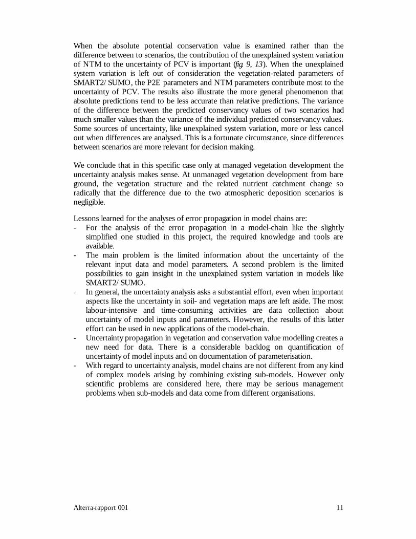
Table 7: Non-zero correlation coefficients

Parameter1 Parameter2 Corr. Coeff.r_e_F b_e_F -0.26r_e_F a_e_F 0.47a_e_F b_e_F -0.92a_pHpH b_e_pHpH -0.97a_e_R b_e_R -0.98

Conversion from pHsms to e_RAs mentioned in section 2.1.3 the pH resulting from SMART2/SUMO refers to thepH in the soil solution (pHsms), whereas the pH used in P2E refers to the pHH2O

(Schouwenberg in prep). Therefore the conversion takes place in two steps: firstconversion of pHsms into pHH2O and secondly conversion of pHH2O into e_R.

Conversion from pHsms of SMART2Sumo to pHH2O

Here we reconsidered the datasets as described in Kros (1998) in order to determinethe uncertainty in both pHsms and pHH2O. The data were restricted to soils sand andclay.

The analyses for sand and clay were combined because the regression coefficientswere much the same. The differences between the residual mean squares, however,0.09314 and 0.1924 respectively, were a bit too large to be ignored. In the combinedanalysis for sand and the inverses of these residual mean squares were used as weight.As was to be expected, the residual mean square of the combined analysis was closeto 1, namely 0.9984. The ensuing residual mean squares, 0.9984*0.09314 for sandand 0.9984*0.1924 for clay, are caused by measurement errors and system variabilityunexplained by the regression. Assuming that the measurement error variance wasapproximately 0.05 for both x_ph and y_ph, and assuming independence ofmeasurement errors, the error variance in y_ph given x_ph was equal to (1+0.87082)* 0.05 = 0.08791. It is obvious that the residual variances were much larger than canbe accounted for by mere measurement errors. Thus, we used σ2

sand = 0.09314-0.08791 = 0.0052, and σ2

clay = 0.1924-0.08791 = 0.1045 as unexplained systemvariation.

New values of pH_water, given pH_soil, were drawn as:

new_pH_water = a_pHpH + b_pHpH*pH_soil + σsoil * ε_pHpH

in which σ2sand = 0.0052 and σ2

clay = 0.1045.

Conversion from pHH2O to e_RThe original parameterisation, using regression of pH on Ellenberg’s e_R, could notsufficiently be reconstructed. Thus, a new parameterisation was constructed.Regression of the Ellenberg indication values on the pH was done, rather than theconverse used originally, because the purpose is to derive Ellenberg indication valuesfrom pH.


The data set for this new parameterisation was obtained from Alterra (Wamelink &Van Dobben 1996).

New cases of e_R, given pH were simulated by

e_R = a_e_R + b_e_R*pH + ε_e_R

The estimates of the regression coefficients, their variances and correlation's describethe parametric uncertainty of the conversion. Normal distributions for bothparameters were assumed, but also a gamma distribution with minimum 0 for theslope coefficient can be used in order to rule completely out the possibility ofnegative slopes (but the probability was already very small under a normaldistribution).

The residual mean square 2.716 is partly caused by the fact that the Ellenbergindication values in the dataset are integers. The variance of the homogeneousdistribution on an interval of length 1 is equal to 1/12. When this variance issubtracted from 2.716 there remains a variance 2.633 caused by measurement errorsand system variability unexplained by the regression. Assuming that themeasurement error is by far the smaller of the two, 2.633 was used as variance of theunexplained system variation.

Conversion from N available to e_NThe original conversion of e_N based on expert judgement could not satisfactory bereconstructed. Therefore for this conversion the uncertainty could not be accountedfor.

3.4.3 NTM

The uncertainty in several regression relations in the SMART2/SUMO-P2E-NTMmodel chain has been defined by the means and covariance-matrix of the regressionestimates. In the case of NTM, however, the situation is somewhat different becauseNTM has not been calibrated via ordinary regression, but via penalised splineregression. In this form of regression, quite a large number of parameters areadapted, and the ensuing risk of overfitting is avoided by means of a penalty forroughness of the response. Thus, the method strikes a balance between the two evilsroughness of the response and infidelity to the data. But the result is that theresponse uncertainty cannot be characterised in the standard way for a small numberof parameters. Instead, the uncertainty in the NTM response, given the Ellenbergnumbers e_F, e_N and e_R, has been characterised in the form of a bootstrapsample of 100 response functions. Thus, a response is defined by a random integerbetween 1 and 100, which will be calculated as 100*uniform(0.1), rounded to thenearest higher integer (see table 8).

But, given the Ellenberg numbers e_F, e_N and e_R, and given the NTM response,the potential nature value is not unique. There is quite some variation that cannot be


accounted for by the regression. The potential nature value has a distribution (forsimplicity assumed to be normal unless this lead to physically impossible response)with the NTM-response as mean, and a variance σ2_NTM.

The potential conservation value (PCV) was calculated as:

new_PCV = fn(e_F, e_N , e_R) + sd_ntm * ε_NTM

in which n = roundup(100*u_NTM), and in which f1 .. . f100 are 100 bootstraprealisations of the NTM response.

sd_ntm = sqrt(10.1277) = 3.18 (heathland); sqrt(5.0025) = 2.24 (deciduous forest);sqrt(2.268)= 1.51 (pine-forest); sqrt(8.955)=2.99 (other)

Table 8: The specified uncertainty distributions of NTM

Name Distribution Mean s.d. min maxu_NTMε_NTM

uniformnormal

-0

-1

0-

1-


4 Methods

In the type of uncertainty analysis applied in this report, uncertainty in a source oferror is modelled by considering this source as a random vector, which is input to themodel. The analysis applied is of the Monte Carlo type, which means that the analysisis based on a random sample from the inputs. The model outputs chosen for analysisare calculated by running the model for each set of values in the sample. Already fora long time, most analyses work like this, but they differ with respect to the way inwhich the sample is constructed, the measures used to express uncertainty anduncertainty contributions, and the actual estimation of these measures. In the lastdecade, these differences tend to become smaller.

Firstly, consensus seems to grow between uncertainty analysts that variances andvariance components are very suitable to characterise output uncertainty anduncertainty contributions.

Secondly, most uncertainty analysts would agree that estimation of uncertaintycontributions of a small number of meaningful groups of inputs is more sensiblethan estimation of uncertainty contributions of a large number of individual (scalar)inputs (in this case: 6 groups instead of 36 individual inputs, see section 3.2).

Thirdly, it is often found embarrassing that many types of uncertainty analyses arebased upon a regression approximation of the model studied. Often, however, theseregression approximations are not entirely successful, and this seriously limits thepossibilities of regression-based uncertainty analysis (see example on p. 39). Themethod of Sobol’ (1990) and the winding stairs method (Jansen et al. 1994) can beused to estimate uncertainty contributions without recourse to regressionapproximations: they are regression-free. The two methods are based on the sameprinciples. Both can be applied in the case of independent groups of inputs; and bothrequire a special type of input sample. In general, regression-free uncertainty analysisrequires larger samples than regression-based analysis. In this report we use thewinding stairs method.

Section 4.1 treats variance-based uncertainty contributions of groups of inputs.Section 4.2 describes the winding stairs method. Section 4.3 discusses the possibilitiesof an alternative method, namely to estimate variance contributions by means oflinear approximations of the sub-models of the chain. An attractive property of thisapproach is that one may perform such an analysis on basis of analyses of theindividual components of the chain: one may study the chain before it exists. Adisadvantage of this approach is that the linear approximations used may beunsatisfactory, implying that the whole method is unsatisfactory.


4.1 Variance-based uncertainty contributions of groups of inputs

In the past, uncertainty, and uncertainty contributions have been expressed in verydiverse measures. In the last decade, however, many uncertainty analysts seem tohave turned to variances and variance components as an uncertainty measure (Sobol’1990; Krzykacz 1990; Jansen et al. 1994; McKay 1996; Jansen 1999; Saltelli et al.1999). This has the great advantage that there is a rich statistical literature on thesubject (e.g. Searle et al. 1992). Moreover, many of the earlier measures can be re-interpreted as variances.

We now define two types of variance-based uncertainty contributions for an arbitrarygroup of inputs (Jansen et al. 1994; Jansen 1999). Let S denote a, possibly pooled,source of uncertainty, and let T denote the group of all other sources of uncertainty.The groups S and T are allowed to be dependent. The model output studied isassumed to depend deterministically on S and T and may thus be written as f(S,T).The total variance, say VTOT, is equal to VTOT = Var[f(S,T)]. The top marginalvariance of S is defined as the expected reduction in output variance if one wouldobtain perfectly certain information about S. No direct information about T willcome in, but if S and T are dependent, some information about T may be conveyedthrough S. Thus, the top-marginal variance of S might be called the part of varianceaccounted for by S. Formally, the top marginal variance of S, TMVS, is defined interms of conditional means and variances:

TMVS = VTOT – E[Var[f(S,T)]|S] = Var[E[f(S,T)|S] .

The bottom marginal variance of S is defined as the output variance that would remain ifone has obtained perfect information about all sources, except S, i.e. perfectinformation about the complementary sources T. The bottom marginal variancemight be called the part of the variance that is not accounted for without S. Theformal definition of the bottom marginal variance of S, BMVS, is as follows:

BMVS = E[Var[f(S,T)|T] .

Note that it follows directly from the above definitions that BMVS and TMVT arecomplementary:

BMVS + TMVT = VTOT.Figure 5 gives an illustration of TMV and BMV. Usually, TMV and BMV areexpressed as percentage of VTOT.In the case that S and T are independent something more can be said. Then, f(S,T) hasthe following analysis of variance decomposition (e.g. Efron & Stein 1981)

f(S,T) = µ + fS(S) + fT(T) + fST(S,T) ,

in which µ is the expectation of f(), whereas µ + fS(S) and µ + fT(T) are conditionalexpectations given S and T respectively, these terms are called the main effects of S andT. The remainder term fST(S,T) is called the interaction of S and T. More formally:


µ = E[f(S,T)] ,µ + fS(S) = E[f(S,T)|S],µ + fT(T) = E[f(S,T)|T].

The top and bottom marginal variances of S may now be expressed as

TMVS = Var[fS(S)] ,BMVS = Var[fS(S)] + Var[fST(S,T)].

Similar expressions may be given for T. Thus, in the case of independent sources,TMVS may be called the main effect variance of S, whereas BMVS may be called the alleffects variance of S. Several other names have been proposed for TMV and BMV,most often in the context of independent sources of uncertainty: importancemeasures, sensitivity estimates, global sensitivity indices. The classical correlationratio is the top marginal variance as fraction of the total variance (Sobol’ 1990;Krzykacz 1990; McKay 1996; Saltelli et al. 1999).

top marginalvariance of S

total variance

bottommarginalvariance of S

nothing knownadditionally

only S knownadditionally

only S unknownadditionally

Figure 5: Graphical representation of total variance VTOT, top-marginal variance of S, TMVS, and bottom-marginal variance of S, BMVS

4.2 Estimation of uncertainty contributions of independent pooledsources

For the definition of uncertainty contributions, it sufficed to discern only a group Sand the complementary group T. For the actual estimation we now consider a scalarmodel output Y = f(A, B, C ...) that depends deterministically on a number of vector


and/or scalar-valued random inputs. We consider the case that the uncertaintysources A, B, C ..., have independent probability distributions. The vectors A, B, C...may have different lengths. Elements of the same vector may be dependent.

The uncertainty contributions of the sources A, B, C... can be estimated by means ofa so-called winding stairs sample. In the box below, a winding stairs sample of f() issketched (figure 6).

Column 1 2 3 ...Row12345678...

f(a1, b1, c1,...) f(a1, b2, c1,...) f(a1, b2, c2,...) ...f(a2, b2, c2,...) f(a2, b3, c2,...) f(a2, b3, c3,...) ...f(a3, b3, c3,...) f(a3, b4, c3,...) f(a3, b4, c4,...) ...f(a4, b4, c4,...) f(a3, b5, c4,...) f(a4, b5, c5,...) ...f(a5, b5, c5,...) f(a5, b6, c5,...) f(a5, b6, c6,...) ...f(a6, b6, c6,...) f(a6, b7, c6,...) f(a6, b7, c7,...) ...f(a7, b7, c7,...) f(a7, b8, c7,...) f(a7, b8, c8,...) ...f(a8, b8, c8,...) f(a8, b9, c8,...) f(a8, b9, c9,...) ......

Figure 6: Sketch of a winding stairs sample of model output f, for independent sources A, B, C.... Independentrandom draws from these sources are indicated by a1, a2..., b1, b2..., c1, c2...

When going through the sample in reading order, one sees that A, B, C... get newvalues in cyclic order. Consecutive elements of the first column contains values of f()for independent draws of all inputs. This column contains information about thetotal variance of f(). The other columns are required to estimate the contributions ofA, B, C... to the total variance.

From a winding stairs sample, the top and bottom marginal variances of A, B, C…may be estimated. For instance, the covariance between columns 1 and 2 of Fig.6 isan estimate of the top marginal variance of B, whereas half the squared differencebetween these columns is an estimate of the bottom marginal variance of B. Othervariances are estimated similarly. The estimates have asymptotic normal distributions.The accuracy of estimates can be assessed through time-series methods. One mayalso estimate the variance of some pools of sources, for instance half the variance ofcolumn 1 minus column 3 is an estimate of the bottom marginal variance of B and Cpooled. Note that the values taken by A,B,C... play no role in the analysis. For moredetails, see Jansen et al. (1994) and Jansen (1999). Sobol’ (1990) proposes a similarway to estimate uncertainty contributions, with the only difference that he uses aslightly different type of sample, in which only one source of uncertainty can beanalysed per sample. The advantage of the winding stairs method is that manysources and pooled sources can be estimated from one sample.

The analysis of this report studies the uncertainty contributions of the 6 groups ofinputs mentioned in Section 3.2. After the quantification of the input uncertaintydescribed in Chapter 2, an ordinary random sample of size 1000 has been drawnfrom the input distribution. This sample was constructed with the Genstat procedure


library USAGE (Jansen & Withagen 1999). Subsequently, this ordinary randomsample was post-processed with Genstat (Genstat 5 Committee 1993) into a windingstairs input sample for 6 groups of inputs: a sample of 6000 sets of inputs. Next, themodel-chain was run for the input sample. This produced a winding stairs samplewith 1000 rows and 6 columns for each of the outputs studied. Finally, these sampleswere analysed with the program WINDINGS (Jansen 1996). The results of theanalysis will be presented in Chapter 5.

4.3 Chain analysis via linear approximations of i/o relations of sub-models

The theory of the previous subsection allows studying the model as a chain by thepooling of the inputs into different groups pertaining to different sub-models in thechain. We now consider an altogether different approach that can be applied if themodel is a chain of known sub-models. Then one can study the chain, before it evenexists, by combining knowledge about the sub-models.

In this section, a vector x of dimension 36 will denote the inputs. The first 24elements of x pertain to SMART2/SUMO; the next 10 are input to P2E, and the last2 to NTM. For a sample of x’s, one may calculate the correspondingSMART2/SUMO outputs pHSMS and Nav. Using these data, one may construct alinear approximation of the outputs by means of two linear least squares regressions.The result can be summarised in matrix form

xCAN

pHSMSSMS

av

SMS +≈

,

in which ASMS is a 2x1 matrix and CSMS is a 2x36 matrix. These matrices contain theregression coefficients; the rows 25...36 of CSMS contain nothing but zeros, becauseSMART2/SUMO is insensitive to the inputs of the other models in the chain, i.e. tox25...x36.

Similarly, one can construct an approximation of the 3 outputs of P2E, given asample of x’s and of values of pHSMS and Nav, for which the P2E outputs e_F, e_Rand e_N have been calculated. Regressions of these 3 outputs on the inputs lead tothe approximation

xCN

pHBA

NeRe

Fe

EPav

SMSEPEP 222

__

_

+

+≈

in which AP2E is a 3x1 matrix and CP2E is a 3x36 matrix. The rows 1...24, 35 and 36 ofCP2E contain only zeros.


The same method applied to NTM output PCV, leads to an approximation of theform

xCNeRe

Fe

BAPCV NTMNTMNTM +

+≈

__

_

where ANTM is a 1x1 matrix and CNTM is a 1x36 matrix. The rows 1...34 of CSMS

contain purely zeros.

The combined linear approximation, obtained by substitution of the second and firstformula in the last, has the form

BxAPCV +≈ ,

in which A is a scalar,

SMSEPNTMePNTMNTM ABBABAA 22 ++= ,

whereas B is a 1x36 matrix representing the sensitivity of the approximation of PCVwith respect to the input vector x:

SMSEPNTMEPNTMNTM CBBCBCB 22 ++= .

Note that the coefficients of the linear approximation BxAPCV +≈ depend ontime and on all model inputs that are absent in x, in particular the hydrological anddeposition scenarios. The linear is far from universal. In theory, one may alsoincorporate the inputs that are absent now, but it is to be expected that this woulddeteriorate the quality of the approximation.

Example. For the case of a rich-sand plot starting with spruce trees in 1995, wecalculated the expected conservation value PCV in 2025, under the business as usualscenario. Since expected conservation value was calculated, there was no unexplainedsystem variation in the NTM inputs: i.e. x35=0. The modelled PCV for the sample ofx’s had mean 9.64 and variance 0.604. The linear approximation calculated asdescribed above also had mean 9.64 but the variance was only 0.340. Thus, 44% ofthe variance of PCV got lost in the linear approximation. This is a bad omen for anuncertainty analysis based on this approximation, since it is the variance that has tobe analysed and ascribed to the different sources of uncertainty: if the object ofanalysis has shrunken so much, there is little ground to assume that the relativeuncertainty contributions are not much altered. Nevertheless, in the current example,uncertainty analysis of the true model and of the linearised version both point tounexplained system variation in P2E as the major source of uncertainty in PCV.


5 Results of the case study

5.1 Overview of the performed analysis

The uncertainty analysis was done by using the program WINDINGS (Jansen 1996).With this program the uncertainty contributions of the different sources (6 groups ofinput data, see section 3.2) can be estimated by means of a so-called winding stairssample (see section 4.2). The analysis was done for the scenario BU to analyse theresults of the model output throughout time. Also an analysis was done to comparethe two scenarios BU and EC. Therefore the differences of the predictions of bothscenarios were used. No separate analysis for the absolute predictions of EC wasdone since differences between scenarios are more relevant for decision making thenthe absolute predictions. The analysis was done for uncontrolled succession frombare ground (succession 1; section 5.2) for the three soil types and a succession fromthe current vegetation (succession 2; section 5.3) for the soil type SR. The analysiswas done without and with accounting for USV of P2E and NTM to get a betterview on the role of USV in the predictions.

The uncertainty contributions of the different sources for the prediction of the PCVare presented in the sections 5.2 and 5.3. An overview of the total analysis, theanalysis of the output of SMART2/SUMO and P2E included, is given in Appendix3. In section 5.4 a summary of the results is presented.


5.2 Uncontrolled succession from bare ground

5.2.1 Analysis without USV

Scenario BUIn figure 7 the results of the analysis of the predictions for the three soiltypes aregiven. In 1995 vegpar, soilpar and p2epar are the main sources of uncertainty,whereas from 2005 onwards, the main source of uncertainty are the vegetation-related parameters. This is mainly caused by the fact that succession takes place frombare ground to forest. There is a huge increase in biomass, resulting in a hugeincrease of N availability (see Appendix 3) and the associated uncertainty in e_N,whereas there is hardly increase in the uncertainty of e_R. Because N availability inSMART2/SUMO is mainly affected by vegpar, it is obvious that the uncertaintycontribution of vegpar increased during the simulation period. In 1995, however, theuncertainty in e_R is relatively high compared to e_N. Consequently parameters thataffecting the soil pH, i.e., soilpar and p2epar, contributed substantially to theuncertainty of the PCV. The uncertainty contribution of soilpar in 1995 increased inthe direction SP > SR > CN (Figure 7a-c).

There is also a clear change in pH during 100 years of succession, although lessextreme than the change in N availability. Which is not surprising, because the pH isa rather stable parameter. More surprisingly, however, is that the pH is increasingunder maintaining the actual deposition, i.e. the BU scenario. This pH increase wascaused by the uncontrolled vegetation succession from bare ground. The increase inbiomass during the succession resulted in an accumulation of N in the vegetation,which in turn yield an additional buffering of acid deposition. Normally, it is foundthat during such simulations the pH decreases in time. This is confirmed by thesimulation of the succession of the current vegetation under the BU scenario. (notshown)

After a decrease of the PCV in the first 10 years of succession, the PCV increases inthe next 90 years. This increase however is not significant (high variances in 2025 and2095). This is caused by the succession from bare ground to forest. In time there isan increase in the uncertainty of the PCV. The prediction of the PCV becomes lessreliable in time. In this case it is mainly caused by the fact that N availability increasesin time and so e_N is in a range of the NTM-matrix in which strong extrapolationtakes place from the range on which the model was calibrated.. The most reliablePCV can be found in the centre of the NTM-matrix. Another factor is the higheruncertainty in the forest submodels compared to the other submodels. This is causedby the fact that less input-data were available for the calibration of these submodels.


Figure 7 a-c: Estimates of the % top-marginal variances for PCV, the BU-scenario, Succession 1 (succession frombare ground), without USV for the soil types non-calcareous clay (7a), Sand Rich (7b) and Sand Poor (7c); abovethe bars the values of the estimates of mean and standard deviation (sd) are given

0.010.020.030.040.050.060.070.080.090.0

100.0

1995 2005 2025 2095

year

estim

ates

% to

p-m

argi

nal v

aria

nces

interactionntmparntmusvp2eusvp2eparsoilparvegpar

13.3 0.3

12.30.4

14.1 2.0

15.5 3.0

soiltype: CNmeansd

7a

0.010.020.030.040.050.060.070.080.090.0

100.0

1995 2005 2025 2095

year

estim

ates

% to

p-m

argi

nal v

aria

nces


13.1 0.3

12.3 0.6

13.4 1.9

15.5 4.0

meansd

soiltype: SR

7b

0.010.020.030.040.050.060.070.080.090.0

100.0

1995 2005 2025 2095

year

estim

ates

% to

p-m

argi

nal v

aria

nces


13.10.3

12.2 0.8

13.4 2.2

16.0 3.3

7c

soiltype: SPmeansd


Difference between the two scenariosFor decision making the relative differences between the predictions of differentscenarios is more important then the absolute predictions. Therefore an analysis wasdone for the difference of the two scenarios (MV-BU). Both scenarios have the sameinput variables at t=0 (1995). So the differences between the predicted values of thetwo scenarios are zero at that time.

The results of the analysis are presented in figure 8. There are no significantdifferences between the two scenarios. It was expected on forehand that the PCV 'sin the EC scenarios would be higher than in the BU scenarios because of the lowerN deposition. The N deposition however is negligible to the increase of biomassduring the succession from bare ground to forest.

As seen in the analysis of the BU scenario the vegetation-related parameters are alsothe main sources of uncertainty for the differences between the two scenarios.

The variance of the differences between the PCV's of the two scenarios have smallervalues than the individual predicted PCV's.


Figure 8: Estimates of the % top-marginal variances for the difference in PCV between the two scenarios (EC-BU), Succession 1, without USV for the soil types non-calcareous clay (8a), Sand Rich (8b) and Sand Poor (8c);above the bars the values of the estimates of mean and standard deviation (sd) are given

0.010.020.030.040.050.060.070.080.090.0

100.0

1995 2005 2025 2095

year

estim

ates

% to

p-m

argi

nal v

aria

nces


0.13 0.2

-1.24 1.05

-0.40 1.46

soiltype: CN

8a

meansd

0.010.020.030.040.050.060.070.080.090.0

100.0

1995 2005 2025 2095

year

estim

ates

% to

p-m

argi

nal v

aria

nces


0.03 0.30

-0.78 0.95

-0.77 2.14

meansd

8b

soiltype: SR

0.010.020.030.040.050.060.070.080.090.0

100.0

1995 2005 2025 2095

year

estim

ates

% to

p-m

argi

nal v

aria

nces


0.070.36

-0.93 1.05

-0.67 1.52

soiltype: SP

8c

meansd


5.2.2 Analysis with USV

Scenario BUBecause the data used for parameterisation of P2E and NTM were still available itwas possible to estimate the USV of both the models. As can be seen in Appendix 2predictions with or without USV can give a dramatic difference. Therefore theWINDINGS analysis was also done with USV.

The results of the analysis are presented in figure 9. The variance is much higher thanthe predictions without USV. The main source of uncertainty is unexplained systemvariation of NTM. Other sources are the unexplained system variation in P2E andthe vegetation-related parameters.


Figure 9: Estimates of the % top-marginal variances for PCV, the BU-scenario, Succession 1 (succession frombare ground), with USV for the soil types non-calcareous clay (9a), Sand Rich (9b) and Sand Poor (9c); abovethe bars the values of the estimates of mean and standard deviation (sd) are given

0.010.020.030.040.050.060.070.080.090.0

100.0

1995 2005 2025 2095

year

estim

ates

% to

p-m

argi

nal v

aria

nces


13.3 3.1

12.7 3.2

12.7 4.2

15.3 4.9

9a

soiltype: CNmeansd

0.010.020.030.040.050.060.070.080.090.0

100.0

1995 2005 2025 2095

year

estim

ates

% to

p-m

argi

nal v

aria

nces


12.0 3.1

12.4 3.1

13.4 3.9

15.1 5.3

9b

meansd

soiltype: SR

0.010.020.030.040.050.060.070.080.090.0

100.0

1995 2005 2025 2095

year

estim

ates

% to

p-m

argi

nal v

aria

nces


13.1 3.1

12.3 3.1

13.4 4.0

15.7 4.8

soiltype: SP

9c

meansd


Difference between the two scenariosThe results of the analysis of the differences of the predictions of the differentscenarios are presented in figure 10.

The analysis of the differences illustrates the phenomenon that absolute predictionstend to be less accurate than the relative predictions. The differences betweenpredicted PCV's of two scenarios have smaller values and variances than individualpredicted PCV's. The several sources of uncertainty more or less cancel out whendifferences are analysed. It can be concluded that USV is not relevant in comparingscenarios.

The USV of P2E however still has to be accounted for. Again the vegetation-relatedparameters are another source of uncertainty.


Figure 10: Estimates of the % top-marginal variances for the difference in PCV between the two scenarios (EC-BU), Succession 1, with USV for the soil types non-calcareous clay (10a), Sand Rich (10b) and Sand Poor(10c); above the bars the values of the estimates of mean and standard deviation (sd) are given

0.010.020.030.040.050.060.070.080.090.0

100.0

1995 2005 2025 2095

year

estim

ates

% to

p-m

argi

nal v

aria

nces


0.02 0.44

-0.95 1.22

-0.37 1.55

10a

soiltype: CNmeansd

0.010.020.030.040.050.060.070.080.090.0

100.0

1995 2005 2025 2095

year

estim

ates

% to

p-m

argi

nal v

aria

nces


0.000.45

-0.62 1.22

-0.73 2.24

10b

soiltype: SRmeansd

0.010.020.030.040.050.060.070.080.090.0

100.0

1995 2005 2025 2095

year

estim

ates

% to

p-m

argi

nal v

aria

nces


0.020.55

-0.79 1.26

-0.65 1.67

meansd

10c

soiltype: SP


5.3 Succession of current vegetation

For the prediction of the PCV of the succession of the current vegetation, spruce-forest, the NTM submodel for pine-forest was used.

5.3.1 Analysis without USV

Scenario BURegarding the predictions for the scenarios for the succession of the currentvegetation, there is a small decrease in pH and N availability. The PCV decreasesslightly in 100 years (see figure 11).

Figure 11: Estimates of the % top-marginal variances for PCV, the BU-scenario, Succession 2 (succession of thecurrent vegetation), without USV. Soiltype: Sand Rich; above the bars the values of the estimates of mean andstandard deviation (sd) are given

In the 1995 and 2005 the vegetation-related parameters are the main sources ofuncertainty. During time there is a huge increase in the uncertainty caused by theparameter uncertainty of NTM. This increase is due to the fact that the abioticconditions are in a range of the NTM-matrix in which strong extrapolation tookplace during the calibration of the pine-forest submodel. For this calibration just asmall number of relevées (n=2505) were available, all more or less located in themiddle of the NTM-matrix.

The influence of the uncertainty of the vegetation-related parameters are muchsmaller than during succession from bare ground because the increase of Navailability (increase in biomass) due to succession is much smaller.

Difference between the two scenariosThe main sources of uncertainty of the differences in the predictions of PCV's arethe vegetation-related parameters and the NTM parameters (figure 12).

0.010.020.030.040.050.060.070.080.090.0

100.0

1995 2005 2025 2095

year

estim

ates

% to

p-m

argi

nal v

aria

nces


10.2 0.3

9.90.3

9.70.3

9.70.6

soiltype: SRmeansd


Figure 12: Estimates of the % top-marginal variances for the difference in PCV between the two scenarios (EC-BU), Succession 2, without USV. Soiltype: Sand Rich; above the bars the values of the estimates of mean andstandard deviation (sd) are given

5.3.2 Analysis with USV

The results of the WINDINGS analysis for the succession from the currentvegetation (spruce-forest) with USV are given in figure 13. It is obvious thatuncertainty contribution of NTMUSV is also in this case the main source ofuncertainty.

Figure 13: Estimates of the % top-marginal variances for PCV, the BU-scenario, Succession 2 (succession of thecurrent vegetation), with USV. Soiltype: Sand Rich; above the bars the values of the estimates of mean andstandard deviation (sd) are given

In the analysis of the differences between the scenarios the USV of NTM disappearsas a source for uncertainty (just like the analysis of succession 1; figure 14).

The USV of P2E and the parameter uncertainty of NTM are still an importantsource of uncertainty.

0.010.020.030.040.050.060.070.080.090.0

100.0

1995 2005 2025 2095

year

estim

ates

% to

p-m

argi

nal v

aria

nces


0.140.00

0.150.14

0.05 0.17 soiltype: SR

meansd

0.010.020.030.040.050.060.070.080.090.0

100.0

1995 2005 2025 2095

year

estim

ates

% to

p-m

argi

nal v

aria

nces


10.2 1.7

9.91.7

9.61.7

9.61.8

soiltype: SRmeansd


Figure 14: Estimates of the % top-marginal variances for the difference in PCV between the two scenarios (EC-BU), Succession 2, with USV. Soiltype: Sand Rich; above the bars the values of the estimates of mean andstandard deviation (sd) are given

5.4 Summary

Table 9 presents a (qualitative) summary of the results of the WINDINGS analysis.Looking at the absolute values of the estimations of the PCV, USV of NTM is animportant source of uncertainty. A different set-up of NTM with more and/ordifferent input variables could possibly lead to better predictions.

Otherwise it may be questioned whether or not one should account for unexplainedsystem variation in NTM. It depends on whether one wishes to predict conservationvalue or potential conservation value. On the other hand, there seems to be littleground for neglecting USV in the conversion model P2E.

The different analyses illustrate that absolute predictions tend to be less accurate thanrelative predictions. In the example, differences between predicted conservationvalues of two scenarios had smaller values than individual predicted conservationvalues. Several sources of uncertainty more or less cancel out when differences areanalysed. This is a fortunate circumstance, since differences between scenarios aremore relevant for decision making.

0.010.020.030.040.050.060.070.080.090.0

100.0

1995 2005 2025 2095

year

estim

ates

% to

p-m

argi

nal v

aria

nces


0.120.00

0.120.14

0.030.20

soiltype: SRmeansd


Table 9: Summary of the results of the WINDINGS analysis for absolute predictions and differences betweenscenarios; Source of uncertainty: +++: very important; ++: important; + sometimes important; blank: notimportant

pHsms Nav e_F e_R e_N PCVAbsolute valuesVegpar + +++ ++ +Soilpar +++P2EparP2EUSV +++ +++ ++NTMUSV +++NTMPAR +DifferencesVegpar ++ +++ ++ +++ +++Soilpar ++ ++P2Epar ++ ++P2EUSV ++NTMUSVNTMPAR +


6 Conclusions

6.1 Uncertainty propagation in the model chain SMART/SUMO-P2E-NTM

Two methods have been explored to study the uncertainty propagation in the modelchain, at first a Monte Carlo type method, the regression free winding stairs analysisand at second a method were variance contributions are estimated by means of linearapproximations of the components in the model chain. The analysis was done by thefirst method.

The results of the uncertainty analysis of this specific chain of models are presentedas the contributions of the various sources to the uncertainty of the potentialconservation value (PCV). The uncertainty in the model results is most relevant forpolicy making when two scenarios are compared. In this case the analysis ends in thefollowing results:- When the unexplained system variation of P2E and NTM (USV) is not taken

into account, the SMART2/SUMO vegetation parameters make the largestcontribution to the uncertainty of PCV at both succession stages (successionfrom bare ground and succession of current vegetation). At succession of thecurrent vegetation, the NTM parameters also contribute to the uncertainty ofPCV; (fig 8, 12)

- When we take into account the unexplained system variation of P2E and NTM,the USV of P2E also contributes to the uncertainty of PCV. This contributiondecreases in the long run; (fig 10, 14)

- There is little influence of the soil type in the case of succession from bareground. We did not examine the influence of soil type in the case of successionof current vegetation.

For vegetation development from bare ground to forest the vegetation structure andthe related nutrient catchment change so radically that the difference in nutrientdeposition related to different scenarios is negligible.

The uncertainty analysis asks a substantial effort, even when important aspects likethe uncertainty in soil- and vegetation maps are left aside. The most labour-intensiveand time-consuming activities are data collection about uncertainty of model inputsand parameters.

In general, regression-free uncertainty analyses require more model runs thanregression-based analyses, but in the example of this paper, a regression based-analysis would have produced seriously biased estimates of uncertainty contributions,since a well-fitting regression approximation could not be obtained because themodel is strongly non-linear. On the other hand, it was no problem to execute the6,000 model runs required for the regression-free analysis performed. Of course, inother situations, the computer time required for a large number of model runs might


become prohibitive, and for efficiency reasons, one might then be forced to acceptthe bias associated with a regression-based uncertainty analysis.

6.2 Lessons learned for analyses of error propagation in model chains

The main problem with linking models is a data problemFor the analysis of the error propagation in a model-chain like the slightly simplifiedone studied in this project, the required knowledge and tools are available. The mainproblem is the limited availability of information about the uncertainty of the relevantinput data and model parameters and the limited knowledge about the model structuralerror of process models

Relative predictions tend to be more accurate then absolute predictionsThe case study illustrates the more general phenomenon that absolute predictions tendto be less accurate than relative predictions. In the example, differences betweenpredicted potential conservancy values of two scenarios had smaller variances thanindividual predicted potential conservancy values. Several sources of uncertainty more orless cancel out when differences are analysed. This is a fortunate circumstance, sincedifferences between scenarios are more relevant for decision making

Unintentional results are valuableNot only the intended results of the analysis are valuable, but also the troublesexperienced when performing the steps of the analysis: the ease with which one makesup an inventory of the sources of uncertainty and quantifies them, forms a check of themanagement of model quality. The analysis also constitutes a test if the model runswithout problems under a wide range of circumstances.

Uncertainty analysis creates a new need for dataUncertainty propagation in vegetation and conservation value modelling creates a newneed for data. So there is a considerable backlog on quantification of uncertainty ofmodel inputs and on documentation of parameterisation.

Model chains are not essentially different from complex modelsModel chains are not essentially different from any kind of complex models. Onlyscientific problems are discussed here. There may be serious management problemshowever when sub-models and data come from different organisations.

As well accumulation of errors as cancelling out may occurAn accumulation of errors may occur when the model chain grows. An analogybetween a sequence of models and a river basin with various branches comes up.The beginning is rather well ordered but when the chain is extended with variousmodules, state variables, parameters and input data, little by little more uncertainty isadded. The uncertainty may partially cancels out however.


6.3 Recommendations for development and uncertainty analysis ofmodel chains

Direction of continuationSince some important sources of uncertainty were neglected up to now, the projectmust have a continuation to include these sources in the analysis. The modelsequence SMART2/SUMO-P2E-NTM is not meant to predict conservation value ina limited number of points but to generate regional or nation wide images ofconservation value. The uncertainties in the input data concerning soil properties andvegetation and the uncertainty in the spatial images that are the output of the modelchain, have to be included in the analysis.

Implementation of the used methodSince the development of a high quality modelling systems is an interest of Alterraand because uncertainty analysis contributes considerable to insight in the reliabilityof model results, a decisive implementation of methods for uncertainty analysis ofmodel sequences is recommended. The method used in this study works well,provided that model runs take little time. Therefore the procedure has to bestreamlined and implemented.

Application of information technologySince there may be serious management problems when sub-models and data fromdifferent organisations are combined, information technology and management toolshave to be applied to manage reliable information exchange.

Data acquisition and model developmentTo solve the problems related to the lack of information about the quality of inputdata and the accuracy of model parameters, the issue of accuracy of model predictionshould get more attention in the data acquisition and model development projects. Awell-documented inventory of sources of uncertainty in the full sequence should bepart of the quality system of the model chain.

Careful definition of model improvement projectsSince absolute predictions tend to be less accurate than relative predictions andbecause increasing the reliability of model results ask for serious effort, theapplication of the model chain has to be considered carefully when projects aredefined to increase reliability of model predictions.


References

Alkemade, J.R.M., J. Wiertz & J.B. Latour 1996 Kalibratie van Ellenberg’s milieu-indicatieschalen aan werkelijk gemeten bodemfactoren. Rapport nr. 711901016,RIVM, Bilthoven

Bal, D., H.M. Beije, Y.R. Hoogeveen, S.R.J. Jansen & P.J. van der Reest 1995.Handboek Natuurdoeltypen in Nederland. Informatie- en Kenniscentrum Natuur-beheer, Ministerie van Landbouw, Natuurbeheer en Visserij. Wageningen.

Clausman, P.H.M.A., W. van Wijngaarden & A.J. den Held 1984. Verspreiding enecologie van wilde planten in Zuid-Holland. Deel A, waarderingsparameters.Provinciale Planologische Dienst Zuid-Holland.

Draper, N.R. & H. Smith 1998. Applied regression analysis (third edition), NewYork: Wiley.

Efron, B. & C. Stein 1981. The jackknife estimate of variance. Ann. Stat. 9 (1981)586-596.

Eilers, P.H.C. & B.D. Marx 1996. Flexible smoothing with B-splines amd penalties.Statistical Science 11: 89-121.

Ellenberg, H., H.E. Weber & R. Duell 1991. Zeigerwerte von Pflanzen inMitteleuropa. Scripta Geobotanica XVIII. Goltze Verlag, Göttingen, Duitsland.

Genstat 5 Committee 1993, Genstat 5 Reference Manual, Oxford : Clarendon Press.

Hertog, A.J. & M. Rijken 1992. Geautomatiseerde bepaling van natuur-behoudswaarde in vegetatieopnamen. Provincie Gelderland, Dienst Ruimte, Wonenen Groen. Intern document.

Jansen, M.J.W., W.A.H. Rossing. & R.A. Daamen 1994. Monte Carlo estimation ofuncertainty contributions from several independent multivariate sources, In:Grasman, J. & G. van Straten (eds.), Predictability and Nonlinear Modelling inNatural Sciences and Economics, p334-343, Kluwer, Dordrecht 1994.

Jansen, M.J.W. 1996. Winding stairs sample analysis program WINDINGS 2.0,Wageningen: DLO-GLW-note MJA-96-2 1996.

Jansen, M.J.W. & J.C.M. Withagen 1999. Usage: uncertainty and sensitivity analysis ina Genstat environment. Manual and Genstat procedures. Version 1.0 ,http://www.cpro.wageningen-ur.nl/cbw/genstat/.


Jansen, M.J.W. 1999. Analysis of variance designs for model output, ComputerPhysics Communications 117, 1999, 35-43.

Klap, J.M., W. de Vries, & E.E.J.M. Leeters. 1998. Effects of acid atmosphericdeposition on the chemical composition of loess, clay and peat soils under forest inThe Netherlands. SC-DLO, Report 97.1, Wageningen, The Netherlands.

Kros, J. 1998. De modellering van de effecten van verzuring, vermesting enverdroging voor bossen en natuurterreinen ten behoeve van de milieubalans,milieuverkenning en natuurverkenning. Verbetering, verfijning en toepassing van hetmodel SMART2 (in Dutch). Wageningen, DLO-Staring Centrum, ReeksMilieuplanbureau 3.

Kros, J., W. de Vries, P.H.M. Janssen, & C.I. Bak. 1993. The uncertainty inforecasting regional trends of forest soil acidification. Water, Air and Soil Pollut.66:29-58.

Kros, J., G.J. Reinds, W. De Vries, J.B. Latour, & M. Bollen. 1995. Modelling of soilacidity and nitrogen availability in natural ecosystems in response to changes in aciddeposition and hydrology. Report 95. DLO Winand Staring Centre, Wageningen,The Netherlands.

Kros, J., E.J. Pebesma, G. J. Reinds & P.A. Finke 1999. Uncertainty in Modelling SoilAcidification at the European Scale, A case study, Journal of Environmental Quality28/2: 366-377

Krzykacz, B. 1990. SAMOS: a computer program for the derivation of empiricalsensitivity measures of results from large computer models, Gesellschaft fürReaktorsicherheit, GRS-A-1700, 1990.

Leeters, E.E.J.M., H. Hartholt, W. de Vries, & L.J.M. Boumans 1993. Effects of aciddeposition on 150 forest stands in The Netherlands. Relationships betweendeposition level, stand and site characteristics and the chemical composition ofneedles, mineral soil, soil solution and groundwater. Report 69.4, DLO WinandStaring Centre, Wageningen, The Netherlands.

Liefveld, W.M., A.H. Prins & G. van Wirdum 1998. Geïntegreerd RuimtelijkEvaluatie-Instrument voor Natuurontwikkelings Scenarios (GREINS).NatuurTechnisch Model (NTM-2) B. Kwantificeren van de indicatieschalen van hetNTM-2 en analyse van de modeloutput van SMART2 en SIMGRO. NBP-Onderzoeksrapport 15. DLO-Instituut voor Bos- en Natuuronderzoek.Wageningen.

McKay, M.D. 1996. Variance-based methods for assessing uncertainty importance inNUREG-1150 analyses, Los Alamos National Laboratory, LA-UR-96-2695.


Oude Voshaar, J.H. 1994. Statistics for researches, with examples from agricultureand environmental sciences [in Dutch], Wageningen Press.

Reinds, G.H. 1994. A data base for European forest soils. Technical DocumentDLOWinand Staring Centre, Wageningen, The Netherlands.

Saltelli A., S. Tarantola & K. Chan 1999. A quantitative, model independent methodfor global sensitivity analysis of model output, Technometrics, 41(1), 39-56.

Schouwenberg, E.P.A.G. in prep. Geïntegreerd Ruimtelijk Evaluatie-Instrumentvoor Natuurontwikkelings Scenario's - Beerze-Reusel(GREINS2). NatuurtechnischModel (NTM 3.0). Alterra-rapport. Alterra, Green World Research, Wageningen.

Searle, S.R., G. Casella & C.E. McCulloch 1992. Variance components, New York:Wiley.

Sobol' I.M. 1990. Sensitivity Estimates for Nonlinear Mathematical Models.Matematicheskoe Modelirovanie 2 (1990) 112-118 [in Russian]; translated inMathematical Modelling and Computational Experiments, 1 (1993) 407-414

Van der Sluis, T. 1996. Vegetatiekundige natuurwaardebepaling. NBP-onderzoekrapport 7. DLO-Instituut voor Bos- en Natuuronderzoek. Wageningen,117 p.

Van Wirdum, G. 1981. Design for a land ecological survey of nature protection. In:S.P. Tjallingii & A.A. De Veer (ed.). Perspectives in land ecology. Pudoc,Wageningen; 245-251.

Wamelink, G.W.W. & H.F. van Dobben 1996. Schatting van responsies van soortenop de milieufactoren vocht, pH en macronutriënten: een aanzet tot calibratie vanEllenberg’s indicatiegetallen. DLO-instituut voor Bos- en natuuronderzoek. Rapport233, Wageningen.

Wamelink, G.W.W., C.J.F. ter Braak & H.F. van Dobben 1997. De Nederlandsenatuur in 2020: schatting van de potentiële natuurwaarde in drie scenario’s. IBN-rapport 312. DLO-Instituut voor Bos- en Natuuronderzoek. Wageningen. 79 p.

Wamelink, G.W.W., J.P. Mol-Dijkstra, H.F. van Dobben, J. Kros & F. Berendse2000. Eerste fase van de ontwikkeling van Successie Model SUMO 1.0. Verbeteringvan de vegetatiemodellering in de Natuurplanner. Alterra-rapport 045. Alterra, GreenWorld Research, Wageningen.

Wamelink, G.W.W., H. van Oene, J.P. Mol-Dijkstra, J. Kros, H.F. van DobbenF. Berendse, 2000 Validatie van de modellen SMART2, SMART2-SUMO1.0,NUCOM en MOVE op site, regionaal en nationaal niveau. Alterra-rapport 65,Alterra, Green World Research, Wageningen.


Wheeler B.D. 1988. Species richness , species rarity and conservation evaluation ofrich-fen vegetation in lowland England and Wales. Journal of Applied Ecology 25:331-353.

Witte, J.P.M. & R. van der Meijden 1992. Verspreiding en natuurwaarden vanecotoopgroepen in Nederland. Onderzoek effecten grondwaterwinning.Rijksinstituut voor Volksgezondheid en Milieuhygiëne, Bilthoven


Annex 1 List of symbols

Symbol Explanation

Amlf Amount of litterfallAmrd Amount of dead rootsBU Business as usual scenarioBMVS see p.36CN Soiltype: non-calcareous clayctNlf Content of Nitrogen in litterfallctNrd Content of Nitrogen in dead rootsDep_Scen Deposition scenarioDrz Thickness of root zoneEC European co-ordination scenarioe_F Ellenberg indication value for moisturee_N Ellenberg indication value for nutrient availabilitye_R Ellenberg indication value for acidity.GT Groundwater table classHyd_Scen Hydrology scenarioMan_Scen Management scenarioMSGL Mean spring groundwater levelNav N available (mol N ha -1 a-1).Nfu foliar uptake of NNru Nitrogen root uptakeNTM Model for the prediction of potential conservation valuentmpar NTM’s response uncertaintyntmusv unexplained system variation in NTMP2E Model for the conversion of physical entities into Ellenberg

indication valuesp2epar Group of P2E parametersp2eusv Group of numbers expressing unexplained system variation

in the conversion model P2EPCV Potential conservation valuepHH2O pH measured in the soil solution obtained by centrifugation

from a freshly taken composite samplepHsms pH according to a standardised soil analysis procedure (i.e.

shaking a dried soil sample with demineralised water using avolume based soil/water of 1:5).

RC Regression coefficientSim_period Simulation periodSMART2 Soil acidification and nutrient cycling modelSMSs SMART2/SUMO-model variables and parameters related to

a soil typeSMSsv SMART2/SUMO-model variables and parameters related to

a soil type and vegetation type


SMSv SMART2/SUMO-model variables and parameters related toa soil type

soilpar group of SMART2/SUMO soil parametersSP Soiltype: Sand poorSR Soiltype: Sand richSUMO Succession modelSUMO_veg_code SUMO vegetation codeTMVS see p. 36USV Unexplained system variationvegpar Group of SMART2/SUMO vegetation parametersVTOT see p. 36


Annex 2 Estimation of uncertainties in P2E and NTM

P2E

To supplement the currently used conversion parameters (Wamelink et. al. 1997)with information about their accuracy was more difficult than expected.

The original parameterisation, using regression of MSGL on Ellenberg’s e_F, couldbe flawlessly reconstructed. Nevertheless, we constructed a new parameterisation.Firstly, in order to avoid predicted values of e_F outside the allowed range from 1 to12, the original regression used a trick which gives rise to some problems when onewishes to assess the covariance matrix of the parameters. Moreover, we preferredregression of the Ellenbergs indication values on MSGL, rather than the converseused originally, because the purpose is to derive Ellenberg scores from pH. Anexponential regression of e_F on MSGL was performed, and doing so the objectionsmentioned were circumvented.

The data set was obtained from RIVM (Alkemade et al. 1996).

To every 10 observations, a fake observation with MSGL=-25 and e_F=1 wasadded, in order to ensure that the fitted curve would be very close to that point whenone extrapolates from the original MSGL range, which has minimum –2.12 forMSGL. Thus, 19 fake observations were added to the original 193 measurements.

The estimates of the regression coefficients, their variances and correlation's describethe parametric uncertainty of the conversion.

The residual mean square 0.6009 is caused by measurement errors and systemvariability unexplained by the regression. Assuming that the measurement error is by farthe smaller of the two, vsys=0.6009 ws used as variance of the unexplained systemvariation.

The most obvious way to draw a new realisation of e_R, would seem to be

new_e_F = a_e_F + b_e_F * r_e_F^MSGL + ε_e_F

in which eps_e_R has mean 0 and variance vsys. But this way a value may fall outsidethe range from 1 to 12; if this occurs, the value is set to the nearest value in therange, i.e. 1 or 12.


Summary

The uncertainty in e_F, given MSGL, is described by the following table

Name distribution mean s.d. min maxr_e_Fb_e_Fa_e_Fε_e_F

normalnormalnormalnormal

1.53316.8501.0690

0.04550.1910.1770.775

----

----

Percentage correlation's between r_e_F, b_e_F, a_e_F R 100.00 B -25.73 100.00 A 46.71 -92.38 100.00 R B AOther correlation's are 0.

New values are drawn as

new_e_F = a_e_F + b_e_F * r_e_F^MSGL + ε_e_F(truncated to range 1-12).

Figure 15: Graph of observations and regression fit on true data range.

observationsregression fit

e_F

MSGL (meters)


Figure 16: Graph of observations and regression fit on fake data range.

Conversion from pHsms to e_RAs mentioned in section 2.1.3 the pH resulting from SMART2/SUMO refers to thepH in the soil solution (pHsms), whereas the pH used in P2E refers to the pHH2O

(Schouwenberg in prep). Therefore the conversion takes place in two steps: firstconversion of pHsms into pHH2O and secondly conversion of pHH2O into e_R.

Conversion from pHsms of SMART2Sumo to pHH2O

Here we reconsidered the datasets as described in Kros (1998) in order to determine theuncertainty in both pHsms and pHH2O. The data were restricted to soils sand and clay.

The analyses for sand and clay were combined because the regression coefficientswere much the same. The differences between the residual mean squares, however,0.09314 and 0.1924 respectively, were a bit too large to be ignored. In the combinedanalysis for sand and the inverses of these residual mean squares were used as weight.As was to be expected the residual mean square of the combined analysis was verynearly equal to 1, namely 0.9984. The ensuing residual mean squares, 0.9984*0.09314for sand and 0.9984*0.1924 for clay, are caused by measurement errors and systemvariability unexplained by the regression. Assuming that the measurement error variancewas approximately 0.05 for both x_pH and y_pH, and assuming independence ofmeasurement errors, the error variance in y_pH given x_pH was equal to(1+0.87082) * 0.05 = 0.08791. It is obvious that the residual variances were muchlarger than can be accounted for by mere measurement errors. Thus, we used σ2

sand =0.09314-0.08791 = 0.0052, and σ2

clay = 0.1924-0.08791 = 0.1045 as unexplainedsystem variation.

MSGL (meters)

e_F

observationsregression fit


Figure 17: Graph of observations and regression fit

Summary

The following table describes the uncertainty in pHH2O, given pHsms

Name Distribution mean s.d. min maxa_pHpHb_pHpHε_pHpH

Normalnormalnormal

0.74240.87080

0.05250.01240.999

---

---

ρ(a_pHpH, b_pHpH) = -0.972; the other correlation's are 0.

New values of pH_water, given pH_soil, were drawn as

new_pH_water = a_pHpH + b_pHpH*pH_soil + σsoil * ε_pHpH

in which σ2sand = 0.0052 and σ2

clay = 0.1045.

Graphs

In the next graph, of observations and regression fit, ‘o’ indicates sand and ‘∆’indicates clay.

pH_H20

pH_soil

observations (sand)observations (clay)regression fit


As seen in figure 4a-b there was a dramatic difference in new realisations of pHH2O,given a set of 1000 given values of pH_soil between the graph with unexplainedsystem variation the graph without unexplained system variation.

Conversion from pHH2O of SMART2Sumo to e_RTo supplement the currently used conversion parameters (Wamelink & Van Dobben1996) with information about their accuracy was more difficult than expected. Theoriginal parameterisation, using regression of pH on Ellenberg’s e_R, could notsufficiently be reconstructed. Thus, a new parameterisation was constructed.Regression of the Ellenberg indication values on the pH was done, rather than theconverse used originally, because the purpose is to derive Ellenberg scores from pH.

The data set for this new parameterisation was prepared as follows.

Summary

New cases of e_R, given pH were simulated by

e_R = a_e_R + b_e_R*pH + ε_e_R

The estimates of the regression coefficients, their variances and correlation's describethe parametric uncertainty of the conversion. Normal distributions for bothparameters were assumed, but also a gamma distribution with minimum 0 for theslope coefficient can be used in order to rule completely out the possibility ofnegative slopes (but the probability was already very small under a normaldistribution).

The residual mean square 2.716 is partly caused by the fact that the Ellenbergindication values in the dataset are integers. The variance of the homogeneousdistribution on an interval of length 1 is equal to 1/12. When this variance issubtracted from 2.716 there remains a variance 2.633 caused by measurement errorsand system variability unexplained by the regression. Assuming that themeasurement error is by far the smaller of the two, 2.633 was used as variance of theunexplained system variation.

The following table describes the distribution.

Name distribution mean Variance Min maxA_e_RB_e_Rε_e_R

normalgammanormal

-0.22150.88760

1.14980.03752.633

-0-

---

ρ(a_e_R, b_e_R) = -0.9835; other correlation's are 0


Figure 18: Graph of observations, regression fit and 1000 newly drawn instances, with given pH homogeneous on3-8.

NTM

Uncertainty in prediction of potential nature value, given the EllenbergnumbersThe uncertainty in several regression relations in the SMART2/SUMO-P2E-NTMmodel chain has been defined by the means and covariance-matrix of the regressionestimates. In the case of NTM, however, the situation is somewhat different becauseNTM has not been calibrated via ordinary regression, but via penalised splineregression. In this form of regression, quite a large number of parameters areadapted, and the ensuing risk of overfitting is avoided by means of a penalty forroughness of the response. Thus, the method strikes a balance between the two evilsroughness of the response and infidelity to the data. But the result is that theresponse uncertainty cannot be characterised in the standard way for a small numberof parameters. Instead, the uncertainty in the NTM response, given the Ellenbergnumbers e_F, e_N and e_R, has been characterised in the form of a bootstrapsample of 100 response functions. Thus, a response is defined by a random integerbetween 1 and 100, which will be calculated as 100*uniform(0.1), rounded to thenearest higher integer.

e_R

pH_H2O

observationsregression fitnewly drawn instances


Given the Ellenberg numbers e_F, e_N and e_R, and given the NTM response, thepotential conservation value is not unique. There is quite some variation that cannotbe accounted for by the regression. The potential nature value has a distribution (forsimplicity assumed to be normal unless this lead to physically impossible response)with the NTM-response as mean, and a variance σ2_NTM.

Summary

new_PCV = fn(e_F, e_N , e_R) + sd_ntm * ε_NTM

in which n = roundup(100*u_NTM), and in which f1 ... f100 are 100 bootstraprealisations of the NTM response.

sd_ntm = sqrt(10.1277) = 3.18 (heather); sqrt(5.0025) = 2.24 (deciduous forest);sqrt(2.268)= 1.51 (pine-forest); sqrt(8.955)=2.99 (other)

Name distribution mean s.d. min maxu_NTMε_NTM

uniformnormal

-0

-1

0-

1-

Correlation's are 0


Annex 3 Results of the WINDINGS analysis

Table I: Estimates of mean and standard deviation (s.d.) for the BU-scenario and succession 1 (bare ground toforest); with and without USV

BU without USV P2E and without USV NTMmsgl pH Navl e_F e_R e_N PCV

- mol ha-1 a-1 - - - -mean s.d. mean s.d. mean s.d. mean s.d. mean s.d. mean s.d. mean s.d.

CN 1995 3 0 5.16 0.20 2270 229 2.99 0.15 4.43 0.41 1.46 0.20 13.3 0.32005 3 0 5.13 0.15 4530 660 2.99 0.15 4.40 0.36 3.40 0.57 12.3 0.52025 3 0 5.27 0.16 8740 1822 2.99 0.15 4.51 0.37 6.94 1.40 14.1 2.02095 3 0 5.48 0.23 17200 4858 2.99 0.15 4.68 0.43 8.79 0.80 15.5 3.0

SP 1995 3 0 4.26 0.22 2180 212 2.99 0.15 3.73 0.32 1.38 0.18 13.1 0.22005 3 0 4.28 0.22 4040 602 2.99 0.15 3.75 0.32 2.98 0.52 12.2 0.92025 3 0 4.33 0.22 7530 1603 2.99 0.15 3.79 0.31 5.98 1.34 13.4 2.22095 3 0 4.52 0.43 16600 4940 2.99 0.15 3.93 0.42 8.72 0.91 16.0 3.3

SR 1995 3 0 4.03 0.29 2160 208 2.99 0.15 3.65 0.37 1.36 0.18 13.1 0.32005 3 0 4.09 0.29 3890 606 2.99 0.15 3.60 0.36 2.85 0.52 12.3 0.62025 3 0 4.20 0.29 7290 1609 2.99 0.15 3.69 0.35 5.77 1.35 13.4 2.02095 3 0 4.49 0.57 15800 1628 2.99 0.15 3.91 0.51 8.56 1.14 15.5 4.0

BU with USV P2E and with USV NTMmsgl pH Nav e_F e_R e_N PCV


CN 1995 3 0 5.16 0.45 2270 229 2.99 0.78 4.44 1.66 1.46 0.20 13.3 3.12005 3 0 5.13 0.39 4530 660 2.99 0.78 4.41 1.65 3.40 0.57 12.7 3.22025 3 0 5.27 0.39 8740 1822 2.99 0.78 4.52 1.65 6.94 1.40 12.7 4.22095 3 0 5.48 0.48 17200 4858 2.99 0.78 4.68 1.72 8.79 0.80 15.3 4.9

SP 1995 3 0 4.26 0.22 2180 212 2.99 0.78 3.76 1.58 1.38 0.18 13.1 3.12005 3 0 4.28 0.22 4040 602 2.99 0.78 3.78 1.58 2.98 0.52 12.3 3.12025 3 0 4.33 0.22 7530 1603 2.99 0.78 3.82 1.58 5.98 1.34 12.3 4.02095 3 0 4.52 0.43 16600 4940 2.99 0.78 3.96 1.61 8.72 0.91 15.7 4.8

SR 1995 3 0 4.03 0.29 2160 208 2.99 0.78 3.60 1.57 1.36 0.18 12.0 3.12005 3 0 4.09 0.29 3890 606 2.99 0.78 3.64 1.57 2.85 0.52 12.4 3.12025 3 0 4.20 0.29 7290 1609 2.99 0.78 3.72 1.58 5.77 1.35 12.4 3.92095 3 0 4.49 0.57 15800 1628 2.99 0.78 3.94 1.63 8.56 1.14 15.1 5.3


Table II: Estimates of the % top-marginal variances of the predictions from Table I; Scenario with and withoutUSV

BU with USV P2E and with USV NTMCN 1995

msgl pH Nav e_F e_R e_N PCVest. s.d. est. s.d. est. s.d. est. s.d. est. s.d. est. s.d. est. s.d.

vegpar - - -2.5 3.1 97.2 4.3 -0.6 3.2 -2.8 3.1 97.1 4.3 2.1 3.0soilpar - - 99.4 4.7 -2.0 3.3 -0.6 3.2 0.9 3.2 -2.0 3.3 1.7 3.0p2epar - - -2.6 3.1 -3.4 3.3 3.5 3.1 -1.0 3.1 -3.5 3.3 1.6 3.1p2eusv - - -2.6 3.1 -3.4 3.3 96.3 4.2 93.3 3.7 -3.5 3.3 8.1 3.1ntmusv - - -2.6 3.1 -3.4 3.3 -0.7 3.2 -2.8 3.1 -3.5 3.3 91.6 4.5ntmpar - - -2.6 3.1 -3.4 3.3 -0.7 3.2 -2.8 3.1 -3.5 3.3 0.8 3.1


msgl pH Navl e_F e_R e_N PCVest. s.d. est. s.d. est. s.d. est. s.d. est. s.d. est. s.d. est. s.d.

vegpar - - -0.5 3.1 93.1 4.5 -0.6 3.2 -0.6 3.2 93.1 4.5 2.1 3.2soilpar - - 93.5 4.9 1.7 3.3 -0.6 3.2 -0.6 3.2 1.7 3.3 -0.5 3.1p2epar - - -1.9 2.9 -4.9 3.2 3.5 3.1 3.5 3.1 -4.9 3.2 0.4 3.0p2eusv - - -1.9 2.9 -4.9 3.2 96.3 4.2 96.3 4.2 -4.9 3.2 8.8 3.1ntmusv - - -1.9 2.9 -4.9 3.2 -0.7 3.2 -1.7 2.4 -4.9 3.2 84.0 4.4ntmpar - - -1.9 2.9 -4.9 3.2 -0.7 3.2 -1.7 2.4 -4.9 3.2 -2.4 3.3



vegpar - - 9.5 3.2 94.2 4.8 -0.6 3.2 -2.1 3.1 93.7 4.1 14.4 3.2soilpar - - 72.9 4.2 1.6 3.5 -0.6 3.2 -0.2 3.2 1.7 3.4 -1.1 3.1p2epar - - -6.5 2.9 -4.0 3.5 3.5 3.1 -0.7 3.1 -3.4 3.5 -0.9 3.0p2eusv - - -6.5 2.9 -0.8 2.4 96.3 4.2 94.4 3.8 -3.4 3.5 19.8 3.1ntmusv - - -6.5 2.9 -0.8 2.4 -0.7 3.2 -2.5 3.1 -3.4 3.5 43.9 3.3ntmpar - - -6.5 2.9 -0.8 2.4 -0.7 3.2 -2.5 3.1 -3.4 3.5 -10.0 3.6



vegpar - - 19.2 3.5 92.0 4.3 -0.6 3.2 -0.4 3.1 92.1 14.3 28.3 3.5soilpar - - 60.5 3.6 -3.9 3.2 -0.6 3.2 0.9 3.1 -6.5 1.5 -2.4 3.0p2epar - - -9.1 3.1 -4.3 3.3 3.5 3.1 -0.7 3.1 -6.1 1.5 -4.6 3.1p2eusv - - -9.1 3.1 -4.3 3.3 96.3 4.2 92.7 3.8 -6.1 1.5 12.9 3.3ntmusv - - -9.1 3.1 -4.3 3.3 -0.7 3.2 -2.8 3.1 -6.1 1.5 27.8 3.2ntmpar - - -9.1 3.1 -4.3 3.3 -0.7 3.2 -2.8 3.1 -6.1 1.5 -10.7 3.5


BU with USV P2E and with USV NTMPS 1995


vegpar - - 3.2 3.0 98.1 4.5 -0.6 3.2 -2.8 3.1 98.1 4.4 2.4 3.0soilpar - - 96.0 4.6 -1.4 3.4 -0.6 3.2 -2.0 3.2 -1.6 3.4 2.1 3.1p2epar - - -1.7 3.1 -3.1 3.4 3.5 3.1 -1.0 0.2 -3.3 3.4 2.1 3.1p2eusv - - -1.7 3.1 -3.1 3.4 96.3 4.2 96.1 3.9 -3.3 3.4 9.3 3.1ntmusv - - -1.7 3.1 -3.1 3.4 -0.7 3.2 -2.8 3.2 -3.3 3.4 90.6 4.4ntmpar - - -1.7 3.1 -3.1 3.4 -0.7 3.2 -2.8 3.2 -3.3 3.4 2.0 3.0



vegpar - - 3.1 3.0 93.1 4.5 -0.6 3.2 -2.7 3.2 93.0 4.5 8.1 3.1soilpar - - 95.5 4.7 0.2 3.3 -0.6 3.2 -2.1 3.2 0.2 3.3 0.2 3.0p2epar - - -2.6 3.1 -7.0 3.3 3.5 3.1 0.1 3.2 -7.0 3.3 -0.2 3.0p2eusv - - -2.6 3.1 -7.0 3.3 96.3 4.2 96.2 3.9 -7.0 3.3 6.4 3.1ntmusv - - -2.6 3.1 -7.0 3.3 -0.7 3.2 -2.8 3.2 -7.0 3.3 78.5 4.4ntmpar - - -2.6 3.1 -7.0 3.3 -0.7 3.2 -2.8 3.2 -7.0 3.3 -1.9 3.2



vegpar - - 6.5 3.1 94.2 4.9 -0.6 3.2 -2.6 3.2 94.4 4.4 23.6 3.2soilpar - - 91.1 4.7 3.5 3.6 -0.6 3.2 -2.2 3.2 3.5 3.6 0.2 3.1p2epar - - -3.5 3.2 -2.1 3.6 3.5 3.1 -0.1 3.2 -1.8 3.6 0.4 3.1p2eusv - - -3.5 3.2 -2.1 3.6 96.3 4.2 96.3 3.9 -1.8 3.6 13.5 3.2ntmusv - - -3.5 3.2 -2.1 3.6 -0.7 3.2 -2.7 3.2 -1.8 3.6 41.9 3.6ntmpar - - -3.5 3.2 -2.1 3.6 -0.7 3.2 -2.7 3.2 -1.8 3.6 -9.8 3.6



vegpar - - 19.7 3.6 91.8 4.0 -0.6 3.2 -1.5 3.2 88.1 11.7 36.2 3.2soilpar - - 52.6 3.6 0.9 3.2 -0.6 3.2 -0.6 3.2 -1.0 3.5 -1.6 3.0p2epar - - -6.5 3.3 0.3 3.1 3.5 3.1 -0.4 3.1 -3.5 2.3 -0.9 3.1p2eusv - - -6.5 3.3 0.3 3.1 96.3 4.2 93.0 3.7 -3.5 2.3 13.5 3.2ntmusv - - -6.5 3.3 0.3 3.1 -0.7 3.2 -2.7 3.3 -3.5 2.3 27.5 3.3ntmpar - - -6.5 3.3 0.3 3.1 -0.7 3.2 -2.7 3.3 -3.5 2.3 -7.2 3.4


BU with USV P2E and with USV NTMRS 1995


vegpar - - 2.9 3.0 96.8 4.4 -0.6 3.2 -2.8 3.2 96.8 4.4 2.4 3.0soilpar - - 95.9 5.2 -0.2 3.4 -0.6 3.2 -1.5 3.3 -0.4 3.5 2.0 3.0p2epar - - -2.0 3.0 -2.9 3.4 3.5 3.1 0.5 3.2 -3.1 3.5 2.1 3.0p2eusv - - -2.0 3.0 -2.9 3.4 96.3 4.2 94.8 3.8 -3.1 3.5 9.3 3.1ntmusv - - -2.0 3.0 -2.9 3.4 -0.7 3.2 -3.0 3.2 -3.1 3.5 90.7 4.4ntmpar - - -2.0 3.0 -2.9 3.4 -0.7 3.2 -3.0 3.2 -3.1 3.5 1.4 3.0



vegpar - - 3.3 3.0 88.2 4.5 -0.6 3.2 -2.8 3.2 88.2 4.5 3.9 3.0soilpar - - 94.6 5.3 4.6 3.3 -0.6 3.2 -1.6 3.2 4.6 3.3 0.0 3.0p2epar - - -2.9 3.0 -6.8 3.2 3.5 3.1 0.4 3.2 -6.8 3.2 0.0 3.0p2eusv - - -2.9 3.0 -6.8 3.2 96.3 4.2 95.1 3.8 -6.8 3.2 5.7 3.1ntmusv - - -2.9 3.0 -6.8 3.2 -0.7 3.2 -2.9 3.2 -6.8 3.2 86.3 4.4ntmpar - - -2.9 3.0 -6.8 3.2 -0.7 3.2 -2.9 3.2 -6.8 3.2 -0.3 3.1



vegpar - - 8.2 3.2 90.9 4.7 -0.6 3.2 -2.4 3.2 91.4 4.4 18.5 3.2soilpar - - 85.9 4.9 5.1 3.5 -0.6 3.2 -1.8 3.2 5.1 3.5 1.0 3.2p2epar - - -4.0 3.0 -2.6 3.5 3.5 3.1 0.1 3.1 -2.3 3.5 0.7 3.1p2eusv - - -4.0 3.0 -2.6 3.5 96.3 4.2 95.3 3.8 -2.3 3.5 9.9 3.3ntmusv - - -4.0 3.0 -2.6 3.5 -0.7 3.2 -2.7 3.2 -2.3 3.5 48.8 3.5ntmpar - - -4.0 3.0 -2.6 3.5 -0.7 3.2 -2.7 3.2 -2.3 3.5 -9.0 3.4



vegpar - - 20.9 3.8 86.1 4.0 -0.6 3.2 -0.6 3.2 83.6 9.1 44.0 3.6soilpar - - 51.9 3.5 -1.8 3.3 -0.6 3.2 0.8 3.2 -0.7 2.9 0.0 3.1p2epar - - -2.4 3.5 -3.3 3.3 3.5 3.1 0.3 3.1 -1.5 3.2 0.2 2.9p2eusv - - -2.4 3.5 -3.3 3.3 96.3 4.2 90.1 3.7 -1.5 3.2 7.8 3.2ntmusv - - -2.4 3.5 -3.3 3.3 -0.7 3.2 -2.7 3.3 -1.5 3.2 23.8 3.1ntmpar - - -2.4 3.5 -3.3 3.3 -0.7 3.2 -2.7 3.3 -1.5 3.2 -6.9 3.4


BU without USV P2E and without USV NTMCN 1995


vegpar - - -2.5 3.1 97.2 4.3 4.4 3.2 -4.6 3.3 97.1 4.3 53.6 10.8soilpar - - 99.4 4.7 -2.0 3.3 4.4 3.2 69.0 3.8 -2.0 3.3 14.3 2.9p2epar - - -2.6 3.1 -3.4 3.3 100 4.6 19.1 3.3 -3.5 3.3 22.3 3.1p2eusv - - -2.6 3.1 -3.4 3.3 4.6 3.2 -4.7 3.2 -3.5 3.3 -5.6 2.7ntmusv - - -2.6 3.1 -3.4 3.3 4.6 3.2 -4.7 3.2 -3.5 3.3 -5.6 2.7ntmpar - - -2.6 3.1 -3.4 3.3 4.6 3.2 -4.7 3.2 -3.5 3.3 -3.7 2.8



vegpar - - -0.5 3.1 93.1 4.5 4.4 3.2 -4.4 3.2 93.1 4.5 71.4 4.3soilpar - - 93.5 4.9 1.7 3.3 4.4 3.2 58.8 3.9 1.7 3.3 -0.6 3.2p2epar - - -1.9 2.9 -4.9 3.2 100 4.6 24.5 3.2 -4.9 3.2 3.1 3.4p2eusv - - -1.9 2.9 -4.9 3.2 4.6 3.2 -5.0 3.1 -4.9 3.2 -5.1 3.1ntmusv - - -1.9 2.9 -4.9 3.2 4.6 3.2 -5.0 3.1 -4.9 3.2 -5.1 3.2ntmpar - - -1.9 2.9 -4.9 3.2 4.6 3.2 -5.0 3.1 -4.9 3.2 -5.0 3.2



vegpar - - 9.5 3.2 94.2 4.8 4.4 3.2 4.3 3.2 93.7 4.1 89.3 3.3soilpar - - 72.9 4.2 1.6 3.5 4.4 3.2 48.3 3.7 1.7 3.4 0.1 3.0p2epar - - -6.5 2.9 -4.0 3.5 100 4.6 22.9 3.4 -3.4 3.5 1.2 3.1p2eusv - - -6.5 2.9 -0.8 2.4 4.6 3.2 -4.7 3.0 -3.4 3.5 -3.3 3.1ntmusv - - -6.5 2.9 -0.8 2.4 4.6 3.2 -4.7 3.0 -3.4 3.5 -3.3 3.1ntmpar - - -6.5 2.9 -0.8 2.4 4.6 3.2 -4.7 3.0 -3.4 3.5 -3.2 3.1



vegpar - - 19.2 3.5 92.0 4.3 4.4 3.2 15.2 3.4 92.1 14.3 85.4 5.8soilpar - - 60.5 3.6 -3.9 3.2 4.4 3.2 45.0 3.6 -6.5 1.5 -0.8 2.9p2epar - - -9.1 3.1 -4.3 3.3 100 4.6 15.7 3.7 -6.1 1.5 -4.2 2.7p2eusv - - -9.1 3.1 -4.3 3.3 4.6 3.2 -4.2 3.1 -6.1 1.5 -5.3 2.6ntmusv - - -9.1 3.1 -4.3 3.3 4.6 3.2 -4.2 3.1 -6.1 1.5 -5.3 2.6ntmpar - - -9.1 3.1 -4.3 3.3 4.6 3.2 -4.2 3.1 -6.1 1.5 -5.1 2.6


BU without USV P2E and without USV NTMPS 1995


vegpar - - 3.2 3.0 98.1 4.5 4.4 3.2 -2.3 2.8 98.1 4.4 37.4 6.2soilpar - - 96.0 4.6 -1.4 3.4 4.4 3.2 24.6 2.8 -1.6 3.4 6.9 3.5p2epar - - -1.7 3.1 -3.1 3.4 100 4.6 67.0 3.8 -3.3 3.4 47.4 3.8p2eusv - - -1.7 3.1 -3.1 3.4 4.6 3.2 -3.8 2.8 -3.3 3.4 -5.2 3.0ntmusv - - -1.7 3.1 -3.1 3.4 4.6 3.2 -3.8 2.8 -3.3 3.4 -5.2 3.0ntmpar - - -1.7 3.1 -3.1 3.4 4.6 3.2 -3.8 2.8 -3.3 3.4 -3.1 3.0



vegpar - - 3.1 3.0 93.1 4.5 4.4 3.2 -2.6 2.8 93.0 4.5 92.6 5.7soilpar - - 95.5 4.7 0.2 3.3 4.4 3.2 24.8 2.8 0.2 3.3 -1.0 3.0p2epar - - -2.6 3.1 -7.0 3.3 100 4.6 66.2 3.8 -7.0 3.3 -1.7 2.9p2eusv - - -2.6 3.1 -7.0 3.3 4.6 3.2 -4.3 2.8 -7.0 3.3 -2.0 2.8ntmusv - - -2.6 3.1 -7.0 3.3 4.6 3.2 -4.3 2.8 -7.0 3.3 -2.0 2.8ntmpar - - -2.6 3.1 -7.0 3.3 4.6 3.2 -4.3 2.8 -7.0 3.3 -2.4 2.8



vegpar - - 6.5 3.1 94.2 4.9 4.4 3.2 -1.2 2.9 94.4 4.4 92.1 4.0soilpar - - 91.1 4.7 3.5 3.6 4.4 3.2 24.3 2.8 3.5 3.6 0.0 3.2p2epar - - -3.5 3.2 -2.1 3.6 100 4.6 64.9 3.8 -1.8 3.6 0.6 3.2p2eusv - - -3.5 3.2 -2.1 3.6 4.6 3.2 -4.1 2.8 -1.8 3.6 -2.3 3.3ntmusv - - -3.5 3.2 -2.1 3.6 4.6 3.2 -4.1 2.8 -1.8 3.6 -2.3 3.3ntmpar - - -3.5 3.2 -2.1 3.6 4.6 3.2 -4.1 2.8 -1.8 3.6 -2.3 3.3



vegpar - - 19.7 3.6 91.8 4.0 4.4 3.2 10.6 3.0 88.1 11.7 91.2 4.1soilpar - - 52.6 3.6 0.9 3.2 4.4 3.2 34.4 3.4 -1.0 3.5 0.7 3.2p2epar - - -6.5 3.3 0.3 3.1 100 4.6 29.3 3.6 -3.5 2.3 1.3 3.3p2eusv - - -6.5 3.3 0.3 3.1 4.6 3.2 -5.9 3.3 -3.5 2.3 -0.3 3.2ntmusv - - -6.5 3.3 0.3 3.1 4.6 3.2 -5.9 3.3 -3.5 2.3 -0.3 3.2ntmpar - - -6.5 3.3 0.3 3.1 4.6 3.2 -5.9 3.3 -3.5 2.3 0.4 3.2


BU without USV P2E and without USV NTMRS 1995


vegpar - - 2.9 3.0 96.8 4.4 4.4 3.2 -1.4 2.9 96.8 4.4 49.4 9.5soilpar - - 95.9 5.2 -0.2 3.4 4.4 3.2 31.9 2.9 -0.4 3.5 7.9 3.1p2epar - - -2.0 3.0 -2.9 3.4 100 4.6 58.5 3.6 -3.1 3.5 35.9 3.2p2eusv - - -2.0 3.0 -2.9 3.4 4.6 3.2 -3.2 2.8 -3.1 3.5 -4.8 2.6ntmusv - - -2.0 3.0 -2.9 3.4 4.6 3.2 -3.2 2.8 -3.1 3.5 -4.8 2.6ntmpar - - -2.0 3.0 -2.9 3.4 4.6 3.2 -3.2 2.8 -3.1 3.5 -3.3 2.7



vegpar - - 3.3 3.0 88.2 4.5 4.4 3.2 -1.4 2.9 88.2 4.5 83.9 4.8soilpar - - 94.6 5.3 4.6 3.3 4.4 3.2 31.5 2.9 4.6 3.3 -0.2 3.2p2epar - - -2.9 3.0 -6.8 3.2 100 4.6 58.1 3.6 -6.8 3.2 3.0 3.3p2eusv - - -2.9 3.0 -6.8 3.2 4.6 3.2 -3.7 2.8 -6.8 3.2 2.1 3.3ntmusv - - -2.9 3.0 -6.8 3.2 4.6 3.2 -3.7 2.8 -6.8 3.2 2.1 3.3ntmpar - - -2.9 3.0 -6.8 3.2 4.6 3.2 -3.7 2.8 -6.8 3.2 2.0 3.3



vegpar - - 8.2 3.2 90.9 4.7 4.4 3.2 0.8 2.9 91.4 4.4 88.0 4.3soilpar - - 85.9 4.9 5.1 3.5 4.4 3.2 30.5 2.9 5.1 3.5 0.6 3.2p2epar - - -4.0 3.0 -2.6 3.5 100 4.6 54.6 3.6 -2.3 3.5 0.5 3.3p2eusv - - -4.0 3.0 -2.6 3.5 4.6 3.2 -3.9 2.8 -2.3 3.5 -2.5 3.3ntmusv - - -4.0 3.0 -2.6 3.5 4.6 3.2 -3.9 2.8 -2.3 3.5 -2.5 3.3ntmpar - - -4.0 3.0 -2.6 3.5 4.6 3.2 -3.9 2.8 -2.3 3.5 -2.5 3.3



vegpar - - 20.9 3.8 86.1 4.0 4.4 3.2 14.5 3.4 83.6 9.1 89.0 4.3soilpar - - 51.9 3.5 -1.8 3.3 4.4 3.2 39.7 3.5 -0.7 2.9 0.0 3.3p2epar - - -2.4 3.5 -3.3 3.3 100 4.6 21.5 3.7 -1.5 3.2 0.1 3.3p2eusv - - -2.4 3.5 -3.3 3.3 4.6 3.2 -3.6 3.5 -1.5 3.2 -0.4 3.3ntmusv - - -2.4 3.5 -3.3 3.3 4.6 3.2 -3.6 3.5 -1.5 3.2 -0.4 3.3ntmpar - - -2.4 3.5 -3.3 3.3 4.6 3.2 -3.6 3.5 -1.5 3.2 -0.4 3.3


Table III: Estimates of mean and standard deviation (s.d.) for the difference between the two scenarios (EC-BU)and succession 1 (bare ground to forest); with and without USV

EC-BU without USV P2E and without USV NTMmsgl pH Nav e_F e_R e_N PCV


CN 1995 0 0 0.00 0.00 0 0 0 0 0.00 0.00 0.00 0.00 0.00 0.002005 0 0 0.02 0.03 -415 84 0 0 0.02 0.02 -0.36 0.07 0.13 0.192025 0 0 0.11 0.16 -1370 506 0 0 0.09 0.12 -1.09 0.42 -1.24 1.052095 0 0 0.14 0.24 -1240 2516 0 0 0.11 0.19 -0.18 0.71 -0.40 1.46

SP 1995 0 0 0.00 0.00 0 0 0 0 0.00 0.00 0.00 0.00 0.00 0.002005 0 0 0.06 0.01 -374 73 0 0 0.04 0.01 -0.32 0.06 0.07 0.362025 0 0 0.15 0.06 -1090 348 0 0 0.12 0.05 -0.93 0.29 -0.93 1.042095 0 0 0.35 0.26 -1520 8216 0 0 0.27 0.21 -0.26 0.77 -0.67 1.51

SR 1995 0 0 0.00 0.00 0 0 0 0 0.00 0.00 0.00 0.00 0.00 0.002005 0 0 0.08 0.02 -356 74 0 0 0.06 0.02 -0.31 0.06 0.03 0.312025 0 0 0.32 0.22 -838 409 0 0 0.24 0.18 -0.71 0.34 -0.78 0.972095 0 0 0.44 0.39 -1390 2891 0 0 0.34 0.31 -0.34 0.86 -0.77 2.14

EC-BU with USV P2E and with USV NTMmsgl pH Nav e_F e_R e_N PCV


CN 1995 0 0 0.00 0.00 0 0 0 0 0.00 0.00 0.00 0.00 0.00 0.002005 0 0 0.02 0.03 -415 84 0 0 0.02 0.02 -0.36 0.07 0.02 0.452025 0 0 0.11 0.16 -1370 506 0 0 0.08 0.12 -1.09 0.42 -0.95 1.222095 0 0 0.14 0.24 -1240 2516 0 0 0.10 0.19 -0.18 0.71 -0.37 1.53

SP 1995 0 0 0.00 0.00 0 0 0 0 0.00 0.00 0.00 0.00 0.00 0.002005 0 0 0.06 0.01 -374 73 0 0 0.04 0.01 -0.32 0.06 0.02 0.532025 0 0 0.15 0.06 -1090 348 0 0 0.11 0.05 -0.93 0.29 -0.79 1.252095 0 0 0.35 0.26 -1520 8216 0 0 0.26 0.07 -0.26 0.77 -0.65 1.66

SR 1995 0 0 0.00 0.00 0 0 0 0 0.00 0.00 0.00 0.00 0.00 0.002005 0 0 0.08 0.02 -356 74 0 0 0.06 0.02 -0.31 0.06 0.00 0.462025 0 0 0.32 0.22 -838 409 0 0 0.23 0.18 -0.71 0.34 -0.62 1.212095 0 0 0.44 0.39 -1390 2891 0 0 0.33 0.31 -0.34 0.86 -0.73 2.24


Table IV: Estimates of the % top-marginal variances of the predictions from table III; Scenario with and withoutUSV

EC-BU without USV P2E and without USV NTMCN 2005


vegpar - - 27.7 5.5 61.5 6.1 - - 25.8 5.0 61.5 6.1 33.3 11.0soilpar - - 38.3 6.7 1.1 3.4 - - 35.8 7.2 1.1 3.4 7.6 6.0p2epar - - 2.5 3.0 -5.3 3.5 - - 1.9 2.7 -5.3 3.5 10.3 2.1p2eusv - - 2.5 3.0 -5.3 3.5 - - 0.7 2.6 -5.3 3.5 1.1 2.4ntmusv - - 2.5 3.0 -5.3 3.5 - - 0.7 2.6 -5.3 3.5 1.1 2.4ntmpar - - 2.5 3.0 -5.3 3.5 - - 0.7 2.6 -5.3 3.5 1.7 2.4



vegpar - - 40.9 7.4 69.6 7.9 - - 37.4 6.2 66.8 8.5 79.0 4.5soilpar - - 24.8 4.1 8.9 3.1 - - 20.7 4.3 10.9 3.1 5.3 2.8p2epar - - -2.4 2.3 -1.9 3.0 - - -1.1 2.6 3.8 2.9 2.3 2.9p2eusv - - -2.4 2.3 -1.9 3.0 - - -1.7 2.4 3.8 2.9 2.0 3.0ntmusv - - -2.4 2.3 -1.9 3.0 - - -1.7 2.4 3.8 2.9 2.0 3.0ntmpar - - -2.4 2.3 -1.9 3.0 - - -1.7 2.4 3.8 2.9 2.1 3.0



vegpar - - 37.6 9.1 55.3 8.3 - - 34.5 9.0 71.8 15.3 32.5 9.1soilpar - - 17.5 3.4 3.7 4.1 - - 15.8 3.5 1.6 2.9 -0.9 1.6p2epar - - -0.9 2.1 -0.8 2.4 - - -0.1 2.4 -0.4 2.9 -7.7 2.4p2eusv - - -0.9 2.1 -0.8 2.4 - - -1.0 2.2 -0.4 2.9 -7.4 2.3ntmusv - - -0.9 2.1 -0.8 2.4 - - -1.0 2.2 -0.4 2.9 -7.4 2.3ntmpar - - -0.9 2.1 -0.8 2.4 - - -1.0 2.2 -0.4 2.9 -7.5 2.4

EC-BU without USV P2E and without USV NTMPS 2005


vegpar - - 31.4 4.0 73.7 7.3 - - 11.3 3.4 73.7 7.3 39.1 11.4soilpar - - 45.8 3.9 3.3 3.2 - - 14.1 3.3 3.3 3.2 -2.4 1.6p2epar - - 1.8 3.3 -1.7 2.9 - - 69.3 3.8 -1.7 2.9 -2.1 1.9p2eusv - - 1.8 3.3 -1.7 2.9 - - 4.3 3.5 -1.7 2.9 -4.5 1.9ntmusv - - 1.8 3.3 -1.7 2.9 - - 4.3 3.5 -1.7 2.9 -4.5 1.9ntmpar - - 1.8 3.3 -1.7 2.9 - - 4.3 3.5 -1.7 2.9 -4.5 1.9




vegpar - - 34.2 5.5 80.4 5.1 - - 27.7 4.7 75.8 4.9 74.6 6.9soilpar - - 34.9 5.2 6.4 3.4 - - 25.9 5.1 7.9 3.1 -0.7 3.1p2epar - - -2.3 3.1 1.3 3.3 - - 23.5 3.3 3.3 3.0 -1.4 3.1p2eusv - - -2.3 3.1 1.3 3.3 - - 0.5 3.4 3.3 3.0 -0.5 3.2ntmusv - - -2.3 3.1 1.3 3.3 - - 0.5 3.4 3.3 3.0 -0.5 3.2ntmpar - - -2.3 3.1 1.3 3.3 - - 0.5 3.4 3.3 3.0 -0.4 3.2



vegpar - - 28.3 3.7 55.0 7.8 - - 26.7 3.7 60.3 10.4 51.4 9.5soilpar - - 13.7 3.5 -0.4 3.0 - - 12.5 3.3 -4.7 2.4 -3.7 2.2p2epar - - 1.7 2.9 -1.2 2.4 - - 9.6 3.2 -4.2 3.0 -3.2 2.2p2eusv - - 1.7 2.9 -1.2 2.4 - - 3.1 3.2 -4.2 3.0 -3.7 1.9ntmusv - - 1.7 2.9 -1.2 2.4 - - 3.1 3.2 -4.2 3.0 -3.7 1.9ntmpar - - 1.7 2.9 -1.2 2.4 - - 3.1 3.2 -4.2 3.0 -3.9 1.8

EC-BU without USV P2E and without USV NTMRS 2005


vegpar - - 30.4 4.5 64.7 8.0 - - 18.2 3.7 64.7 8.0 38.9 9.2soilpar - - 46.4 4.2 6.4 3.3 - - 21.7 3.4 6.4 3.3 -3.0 1.3p2epar - - -3.7 3.1 4.3 3.0 - - 44.9 3.3 4.3 3.0 0.1 1.3p2eusv - - -3.7 3.1 4.3 3.0 - - -1.1 3.4 4.3 3.0 -2.4 1.4ntmusv - - -3.7 3.1 4.3 3.0 - - -1.1 3.4 4.3 3.0 -2.4 1.4ntmpar - - -3.7 3.1 4.3 3.0 - - -1.1 3.4 4.3 3.0 -2.4 1.4



vegpar - - 22.4 4.2 41.2 4.6 - - 20.5 4.1 38.2 4.2 64.5 5.1soilpar - - 42.9 5.4 20.9 3.5 - - 38.7 5.7 21.2 3.4 -1.1 3.1p2epar - - -0.7 3.6 3.7 3.3 - - 10.7 3.9 5.0 2.9 0.1 3.2p2eusv - - -0.7 3.6 3.7 3.3 - - 2.3 3.7 5.0 2.9 1.6 3.3ntmusv - - -0.7 3.6 3.7 3.3 - - 2.3 3.7 5.0 2.9 1.6 3.3ntmpar - - -0.7 3.6 3.7 3.3 - - 2.3 3.7 5.0 2.9 1.4 3.3




vegpar - - 22.2 4.3 42.1 7.1 - - 20.1 4.1 58.6 8.8 46.6 8.0soilpar - - 10.3 3.4 -0.9 3.0 - - 6.8 3.4 -0.2 2.3 2.2 3.8p2epar - - 5.2 3.0 4.1 2.9 - - 11.0 3.1 2.6 2.7 4.3 3.4p2eusv - - 5.2 3.0 4.1 2.9 - - 5.4 3.0 2.6 2.7 4.6 3.4ntmusv - - 5.2 3.0 4.1 2.9 - - 5.4 3.0 2.6 2.7 4.6 3.4ntmpar - - 5.2 3.0 4.1 2.9 - - 5.4 3.0 2.6 2.7 4.5 3.6

EC-BU with USV P2E and with USV NTMCN 2005


vegpar - - 27.7 5.5 61.5 6.1 - - 24.5 5.1 61.5 6.1 13.7 9.1soilpar - - 38.3 6.7 1.1 3.4 - - 35.6 7.2 1.1 3.4 0.8 2.4p2epar - - 2.5 3.0 -5.3 3.5 - - 1.7 2.8 -5.3 3.5 3.3 2.8p2eusv - - 2.5 3.0 -5.3 3.5 - - 1.7 2.7 -5.3 3.5 28.6 3.6ntmusv - - 2.5 3.0 -5.3 3.5 - - 0.0 2.5 -5.3 3.5 0.3 2.3ntmpar - - 2.5 3.0 -5.3 3.5 - - 0.0 2.5 -5.3 3.5 -0.4 2.0



vegpar - - 40.9 7.4 69.6 7.9 - - 37.3 6.2 66.8 8.5 31.7 3.4soilpar - - 24.8 4.1 8.9 3.1 - - 20.4 4.3 10.9 3.1 -0.1 2.8p2epar - - -2.4 2.3 -1.9 3.0 - - -0.7 2.7 3.8 2.9 -1.5 3.1p2eusv - - -2.4 2.3 -1.9 3.0 - - -0.8 2.4 3.8 2.9 12.5 3.0ntmusv - - -2.4 2.3 -1.9 3.0 - - -1.5 2.4 3.8 2.9 -1.2 2.5ntmpar - - -2.4 2.3 -1.9 3.0 - - -1.5 2.4 3.8 2.9 -1.5 2.4



vegpar - - 37.6 9.1 55.3 8.3 - - 33.1 9.3 71.8 15.3 27.3 8.5soilpar - - 17.5 3.4 3.7 4.1 - - 16.9 3.6 1.6 2.9 1.1 1.8p2epar - - -0.9 2.1 -0.8 2.4 - - 0.6 2.5 -0.4 2.9 -6.7 2.4p2eusv - - -0.9 2.1 -0.8 2.4 - - -0.1 2.3 -0.4 2.9 -6.8 2.4ntmusv - - -0.9 2.1 -0.8 2.4 - - -1.1 2.2 -0.4 2.9 -5.7 2.0ntmpar - - -0.9 2.1 -0.8 2.4 - - -1.1 2.2 -0.4 2.9 -6.0 2.1


EC-BU with USV P2E and with USV NTMPS 2005


vegpar - - 31.4 4.0 73.7 7.3 - - 10.6 3.0 73.7 7.3 18.1 7.8soilpar - - 45.8 3.9 3.3 3.2 - - 10.5 2.9 3.3 3.2 0.6 1.9p2epar - - 1.8 3.3 -1.7 2.9 - - 37.3 3.8 -1.7 2.9 0.0 2.1p2eusv - - 1.8 3.3 -1.7 2.9 - - 33.9 5.2 -1.7 2.9 13.0 2.0ntmusv - - 1.8 3.3 -1.7 2.9 - - 4.5 3.1 -1.7 2.9 -2.0 1.7ntmpar - - 1.8 3.3 -1.7 2.9 - - 4.5 3.1 -1.7 2.9 -0.8 1.9



vegpar - - 34.2 5.5 80.4 5.1 - - 22.8 4.7 75.8 4.9 37.0 6.3soilpar - - 34.9 5.2 6.4 3.4 - - 21.8 4.8 7.9 3.1 -0.8 2.5p2epar - - -2.3 3.1 1.3 3.3 - - 16.6 3.5 3.3 3.0 -1.2 2.8p2eusv - - -2.3 3.1 1.3 3.3 - - 13.4 3.6 3.3 3.0 10.6 2.7ntmusv - - -2.3 3.1 1.3 3.3 - - 0.0 3.4 3.3 3.0 -4.0 2.5ntmpar - - -2.3 3.1 1.3 3.3 - - 0.0 3.4 3.3 3.0 -3.4 2.6



vegpar - - 28.3 3.7 55.0 7.8 - - 26.2 3.7 60.3 10.4 39.9 9.3soilpar - - 13.7 3.5 -0.4 3.0 - - 12.5 3.3 -4.7 2.4 -4.5 2.5p2epar - - 1.7 2.9 -1.2 2.4 - - 9.7 3.4 -4.2 3.0 -5.5 2.2p2eusv - - 1.7 2.9 -1.2 2.4 - - 7.2 3.1 -4.2 3.0 -3.7 1.5ntmusv - - 1.7 2.9 -1.2 2.4 - - 4.1 3.1 -4.2 3.0 -1.4 1.3ntmpar - - 1.7 2.9 -1.2 2.4 - - 4.1 3.1 -4.2 3.0 -1.4 1.3

EC-BU with USV P2E and with USV NTMRS 2005


vegpar - - 30.4 4.5 64.7 8.0 - - 13.0 3.3 64.7 8.0 28.3 8.2soilpar - - 46.4 4.2 6.4 3.3 - - 12.4 3.2 6.4 3.3 -3.0 2.5p2epar - - -3.7 3.1 4.3 3.0 - - 23.5 3.5 4.3 3.0 -0.8 2.5p2eusv - - -3.7 3.1 4.3 3.0 - - 27.0 4.4 4.3 3.0 13.8 2.2ntmusv - - -3.7 3.1 4.3 3.0 - - -0.6 3.0 4.3 3.0 1.0 1.7ntmpar - - -3.7 3.1 4.3 3.0 - - -0.6 3.0 4.3 3.0 0.1 1.7




vegpar - - 22.4 4.2 41.2 4.6 - - 16.1 3.7 38.2 4.2 32.5 6.2soilpar - - 42.9 5.4 20.9 3.5 - - 34.4 5.5 21.2 3.4 -2.0 3.0p2epar - - -0.7 3.6 3.7 3.3 - - 8.6 4.0 5.0 2.9 2.0 3.1p2eusv - - -0.7 3.6 3.7 3.3 - - 7.2 3.7 5.0 2.9 11.3 3.4ntmusv - - -0.7 3.6 3.7 3.3 - - 1.6 3.6 5.0 2.9 -0.6 2.9ntmpar - - -0.7 3.6 3.7 3.3 - - 1.6 3.6 5.0 2.9 -1.5 2.8



vegpar - - 22.2 4.3 42.1 7.1 - - 18.2 4.0 58.6 8.8 36.2 7.7soilpar - - 10.3 3.4 -0.9 3.0 - - 5.7 3.4 -0.2 2.3 3.6 3.6p2epar - - 5.2 3.0 4.1 2.9 - - 7.5 3.1 2.6 2.7 4.5 3.4p2eusv - - 5.2 3.0 4.1 2.9 - - 6.5 3.0 2.6 2.7 5.8 3.8ntmusv - - 5.2 3.0 4.1 2.9 - - 4.2 3.0 2.6 2.7 4.5 3.1ntmpar - - 5.2 3.0 4.1 2.9 - - 4.2 3.0 2.6 2.7 4.2 3.0


Table V: Estimates of mean and standard deviation (s.d.) for the BU-scenario and succession 2 (succession ofcurrent vegetation) on rich sand; with and without USV

Bu_S2 with USV P2E and with USV NTMmsgl pH Nav e_F e_R e_N PCV


RS 1995 3 0 4.04 0.30 3830 429 2.99 0.78 3.60 1.57 2.80 0.37 10.2 1.72005 3 0 4.07 0.29 4840 884 2.99 0.78 3.62 1.57 3.67 0.76 9.9 1.72025 3 0 4.09 0.27 6670 1572 2.99 0.78 3.64 1.57 5.23 1.29 9.6 1.72095 3 0 4.13 0.26 11000 2583 2.99 0.78 3.67 1.57 8.09 1.20 9.6 1.8

Bu_S2 without USV P2E and without USV NTMmsgl pH Nav e_F e_R e_N PCV


RS 1995 3 0 4.04 0.30 3830 429 2.99 0.15 3.56 0.37 2.80 0.37 10.2 0.42005 3 0 4.07 0.29 4840 884 2.99 0.15 3.67 0.76 3.67 0.76 9.9 0.32025 3 0 4.09 0.27 6670 1572 2.99 0.15 3.60 0.36 5.23 1.29 9.7 0.42095 3 0 4.13 0.26 11000 2583 2.99 0.15 3.63 0.35 8.09 1.20 9.7 0.6

Table VI: Estimates of the % top-marginal variances of the predictions from Table V; with and without USV

BU_S2 with USV P2E and with USV NTMRS 1995


vegpar - - 1.4 3.1 88.1 4.9 -0.6 3.2 -2.9 3.2 88.1 4.9 3.3 3.0soilpar - - 96.2 5.3 9.4 3.5 -0.6 3.2 -1.6 3.3 9.4 3.5 0.2 3.1p2epar - - -2.5 3.1 -0.8 3.2 3.5 3.1 0.4 3.2 -0.8 3.2 0.2 3.1p2eusv - - -2.5 3.1 -0.8 3.2 96.3 4.2 94.8 3.8 -0.8 3.2 21.2 3.1ntmusv - - -2.5 3.1 -0.8 3.2 -0.7 3.2 -3.0 3.2 -0.8 3.2 74.7 4.1ntmpar - - -2.5 3.1 -0.8 3.2 -0.7 3.2 -3.0 3.2 -0.8 3.2 1.3 3.1



vegpar - - 2.2 3.1 87.5 5.2 -0.6 3.2 -2.9 3.2 87.5 5.2 1.8 3.0soilpar - - 96.2 5.4 12.8 3.4 -0.6 3.2 -1.7 3.2 12.8 3.4 -0.5 3.0p2epar - - -2.3 3.1 1.3 3.2 3.5 3.1 0.4 3.2 1.3 3.2 -0.3 3.1p2eusv - - -2.3 3.1 1.3 3.2 96.3 4.2 95.0 3.8 1.3 3.2 19.1 3.1ntmusv - - -2.3 3.1 1.3 3.2 -0.7 3.2 -3.0 3.2 1.3 3.2 77.6 4.2ntmpar - - -2.3 3.1 1.3 3.2 -0.7 3.2 -3.0 3.2 1.3 3.2 1.8 3.2




vegpar - - 2.9 3.1 87.9 5.8 -0.6 3.2 -2.8 3.2 87.7 4.2 0.3 3.1soilpar - - 93.8 5.4 14.0 3.5 -0.6 3.2 -1.9 3.2 13.7 3.3 -1.7 3.0p2epar - - -3.3 3.1 2.0 3.0 3.5 3.1 0.3 3.2 2.0 3.0 -1.2 3.0p2eusv - - -3.3 3.1 2.0 3.0 96.3 4.2 95.3 3.8 2.0 3.0 14.5 3.1ntmusv - - -3.3 3.1 2.0 3.0 -0.7 3.2 -3.0 3.2 2.0 3.0 79.6 4.3ntmpar - - -3.3 3.1 2.0 3.0 -0.7 3.2 -3.0 3.2 2.0 3.0 2.5 3.2



vegpar - - 10.9 3.1 93.1 4.5 -0.6 3.2 -2.6 3.3 94.4 4.9 -1.6 2.9soilpar - - 79.7 5.0 -2.6 3.2 -0.6 3.2 -2.0 3.2 0.2 3.1 -2.0 2.9p2epar - - -4.8 3.1 -5.4 3.4 3.5 3.1 0.6 3.2 -1.5 3.1 -2.1 3.0p2eusv - - -4.8 3.1 -5.4 3.4 96.3 4.2 95.3 3.8 -1.5 3.1 13.7 3.2ntmusv - - -4.8 3.1 -5.4 3.4 -0.7 3.2 -3.0 3.3 -1.5 3.1 74.7 4.1ntmpar - - -4.8 3.1 -5.4 3.4 -0.7 3.2 -3.0 3.3 -1.5 3.1 10.6 3.0

RS_S2 without USV P2E and without USV NTMCN 1995


vegpar - - 1.4 3.1 88.1 4.9 4.4 3.2 -1.8 2.9 88.1 4.9 50.3 3.6soilpar - - 96.2 5.3 9.4 3.5 4.4 3.2 32.5 2.9 9.4 3.5 2.8 2.8p2epar - - -2.5 3.1 -0.8 3.2 100 4.6 57.7 3.7 -0.8 3.2 30.6 2.9p2eusv - - -2.5 3.1 -0.8 3.2 4.6 3.2 -3.3 2.8 -0.8 3.2 -2.2 3.0ntmusv - - -2.5 3.1 -0.8 3.2 4.6 3.2 -3.3 2.8 -0.8 3.2 -2.2 3.0ntmpar - - -2.5 3.1 -0.8 3.2 4.6 3.2 -3.3 2.8 -0.8 3.2 8.5 3.1

BU_S2 without USV P2E and without USV NTMRS 2005


vegpar - - 2.2 3.1 87.5 5.2 4.4 3.2 -1.4 2.9 87.5 5.2 32.2 3.9soilpar - - 96.2 5.4 12.8 3.4 4.4 3.2 31.5 2.9 12.8 3.4 2.3 2.8p2epar - - -2.3 3.1 1.3 3.2 100 4.6 59.2 3.7 1.3 3.2 33.1 2.9p2eusv - - -2.3 3.1 1.3 3.2 4.6 3.2 -3.1 2.8 1.3 3.2 1.3 3.0ntmusv - - -2.3 3.1 1.3 3.2 4.6 3.2 -3.1 2.8 1.3 3.2 1.3 3.0ntmpar - - -2.3 3.1 1.3 3.2 4.6 3.2 -3.1 2.8 1.3 3.2 17.7 3.1




vegpar - - 2.9 3.1 87.9 5.8 4.4 3.2 -1.5 2.9 87.7 4.2 16.1 3.6soilpar - - 93.8 5.4 14.0 3.5 4.4 3.2 28.6 2.9 13.7 3.3 -1.3 2.7p2epar - - -3.3 3.1 2.0 3.0 100 4.6 61.0 3.8 2.0 3.0 13.7 2.7p2eusv - - -3.3 3.1 2.0 3.0 4.6 3.2 -3.6 2.8 2.0 3.0 0.9 2.7ntmusv - - -3.3 3.1 2.0 3.0 4.6 3.2 -3.6 2.8 2.0 3.0 0.9 2.7ntmpar - - -3.3 3.1 2.0 3.0 4.6 3.2 -3.6 2.8 2.0 3.0 41.0 3.7



vegpar - - 10.9 3.1 93.1 4.5 4.4 3.2 1.0 2.8 94.4 4.9 1.2 2.7soilpar - - 79.7 5.0 -2.6 3.2 4.4 3.2 23.3 2.9 0.2 3.1 -4.6 2.7p2epar - - -4.8 3.1 -5.4 3.4 100 4.6 61.2 3.8 -1.5 3.1 -0.6 2.9p2eusv - - -4.8 3.1 -5.4 3.4 4.6 3.2 -4.5 2.8 -1.5 3.1 -2.7 2.8ntmusv - - -4.8 3.1 -5.4 3.4 4.6 3.2 -4.5 2.8 -1.5 3.1 -2.7 2.8ntmpar - - -4.8 3.1 -5.4 3.4 4.6 3.2 -4.5 2.8 -1.5 3.1 75.4 3.9


Table VII: Estimates of mean and standard deviation (s.d.) for the difference between the two scenarios (EC-BU)and succession 2 (succession of current vegetation) on rich sand; with and without USV

EC-BU_S2 with USV P2E and with USV NTMmsgl pH Nav e_F e_R e_N PCV


RS 1995 0 0 0.00 0.00 0 0 0.00 0.00 0.00 0.00 0.00 0.00 0.00 0.002005 0 0 0.07 0.01 -341 50 0.00 0.00 0.05 0.02 -0.29 0.04 0.12 0.102025 0 0 0.17 0.04 -716 218 0.00 0.00 0.12 0.05 -0.61 0.19 0.12 0.152095 0 0 0.27 0.12 -988 860 0.00 0.00 0.20 0.11 -0.43 0.52 0.03 0.19

EC-BU_S2 without USV P2E and without USV NTMmsgl pH Nav e_F e_R e_N PCV


RS 1995 0 0 0.00 0.00 0 0 0.00 0.00 0.00 0.00 0.00 0.00 0.00 0.002005 0 0 0.07 0.01 -341 50 0.00 0.00 0.06 0.02 -0.29 0.04 0.14 0.102025 0 0 0.17 0.04 -716 218 0.00 0.00 0.13 0.04 -0.61 0.19 0.15 0.142095 0 0 0.27 0.12 -988 860 0.00 0.00 0.21 0.10 -0.43 0.52 0.05 0.18

Table VIII: Estimates of the % of top-marginal variances of the predictions from Table VII; with and withoutUSV

EC-BU_S2 with USV P2E and with USV NTMRS 2005


vegpar - - 56.7 5.0 93.3 4.6 - - 14.8 3.2 93.3 4.6 47.8 3.3soilpar - - 25.2 3.1 1.7 2.9 - - 2.4 3.1 1.7 2.9 10.1 3.0p2epar - - -4.3 3.1 0.0 2.9 - - 28.6 3.9 0.0 2.9 3.2 3.1p2eusv - - -4.3 3.1 0.0 2.9 - - 31.6 4.9 0.0 2.9 25.1 3.1ntmusv - - -4.3 3.1 0.0 2.9 - - 1.2 3.0 0.0 2.9 1.0 3.0ntmpar - - -4.3 3.1 0.0 2.9 - - 1.2 3.0 0.0 2.9 9.1 3.2



vegpar - - 50.2 17.7 78.6 5.2 - - 19.3 6.0 76.2 5.0 24.1 3.4soilpar - - 34.0 7.3 5.1 4.0 - - 10.6 2.8 2.5 3.5 -2.3 2.7p2epar - - 3.9 3.3 -0.7 3.4 - - 25.6 3.6 -0.2 3.0 1.3 2.8p2eusv - - 3.9 3.3 -0.7 3.4 - - 26.5 4.4 -0.2 3.0 13.6 3.1ntmusv - - 3.9 3.3 -0.7 3.4 - - 5.0 2.9 -0.2 3.0 3.2 2.8ntmpar - - 3.9 3.3 -0.7 3.4 - - 5.0 2.9 -0.2 3.0 24.9 3.1




vegpar - - 29.6 5.8 85.4 3.0 - - 21.2 4.0 75.2 3.8 20.3 4.3soilpar - - 18.0 4.9 -1.0 3.1 - - 10.6 4.2 7.3 3.3 -4.2 3.1p2epar - - 1.8 3.0 0.9 3.0 - - 15.5 4.1 1.1 3.1 -4.6 2.8p2eusv - - 1.8 3.0 0.9 3.0 - - 15.2 3.7 1.1 3.1 3.0 3.1ntmusv - - 1.8 3.0 0.9 3.0 - - 5.2 3.3 1.1 3.1 -5.4 3.3ntmpar - - 1.8 3.0 0.9 3.0 - - 5.2 3.3 1.1 3.1 14.3 3.1

EC-BU_S2 without USV P2E and without USV NTMRS 2005


vegpar - - 56.7 5.0 93.3 4.6 - - 23.2 3.5 93.3 4.6 77.3 3.5soilpar - - 25.2 3.1 1.7 2.9 - - 7.0 3.2 1.7 2.9 6.7 3.1p2epar - - -4.3 3.1 0.0 2.9 - - 61.6 3.9 0.0 2.9 -0.1 3.1p2eusv - - -4.3 3.1 0.0 2.9 - - -0.8 3.5 0.0 2.9 -1.6 3.1ntmusv - - -4.3 3.1 0.0 2.9 - - -0.8 3.5 0.0 2.9 -1.6 3.0ntmpar - - -4.3 3.1 0.0 2.9 - - -0.8 3.5 0.0 2.9 10.4 3.2



vegpar - - 50.2 17.7 78.6 5.2 - - 25.0 7.3 76.2 5.0 35.3 4.1soilpar - - 34.0 7.3 5.1 4.0 - - 15.4 2.9 2.5 3.5 -1.7 3.1p2epar - - 3.9 3.3 -0.7 3.4 - - 47.8 3.4 -0.2 3.0 0.5 2.9p2eusv - - 3.9 3.3 -0.7 3.4 - - 2.8 3.5 -0.2 3.0 -1.5 3.0ntmusv - - 3.9 3.3 -0.7 3.4 - - 2.8 3.5 -0.2 3.0 -1.5 3.0ntmpar - - 3.9 3.3 -0.7 3.4 - - 2.8 3.5 -0.2 3.0 28.5 3.2



vegpar - - 29.6 5.8 85.4 3.0 - - 21.4 4.1 75.2 3.8 32.2 4.2soilpar - - 18.0 4.9 -1.0 3.1 - - 11.6 4.6 7.3 3.3 -3.6 3.5p2epar - - 1.8 3.0 0.9 3.0 - - 22.8 4.0 1.1 3.1 -6.6 3.2p2eusv - - 1.8 3.0 0.9 3.0 - - 2.9 3.3 1.1 3.1 -8.1 3.3ntmusv - - 1.8 3.0 0.9 3.0 - - 2.9 3.3 1.1 3.1 -8.1 3.3ntmpar - - 1.8 3.0 0.9 3.0 - - 2.9 3.3 1.1 3.1 15.3 3.1

Uncertainty propagation in model chains: a case...

Documents

Transcript of Uncertainty propagation in model chains: a case...