ULTIMATE STRENGTH ANALYSIS OF STIFFENED … · based on a further extension of the nonlinear...
169
ULTIMATE STRENGTH ANALYSIS OF STIFFENED PANELS USING A BEAM-COLUMN METHOD Yong Chen Dissertation submitted to the Faculty of the Virginia Polytechnic Institute and State University in partial fulfillment of the requirements for the degree of Doctor of Philosophy In Aerospace Engineering Dr. Owen F. Hughes, Chair Dr. Michael J. Allen Dr. Alan J. Brown Dr. Eric Johnson Dr. Rakesh K. Kapania January 15, 2003 Blacksburg, Virginia Keywords: Ultimate Strength, Stiffened Panels, Beam-column Method, Orthotropic Plate Method Copyright 2003, Yong Chen
-
Upload
phungquynh -
Category
Documents
-
view
219 -
download
0
Transcript of ULTIMATE STRENGTH ANALYSIS OF STIFFENED … · based on a further extension of the nonlinear...
ULTIMATE STRENGTH ANALYSIS OF STIFFENED PANELS USING A BEAM-COLUMN METHOD
Yong Chen
Dissertation submitted to the Faculty of the
Virginia Polytechnic Institute and State University
in partial fulfillment of the requirements for the degree of
Doctor of Philosophy
In
Aerospace Engineering
Dr. Owen F. Hughes, Chair
Dr. Michael J. Allen
Dr. Alan J. Brown
Dr. Eric Johnson
Dr. Rakesh K. Kapania
January 15, 2003
Blacksburg, Virginia
Keywords: Ultimate Strength, Stiffened Panels, Beam-column Method,
Orthotropic Plate Method
Copyright 2003, Yong Chen

ULTIMATE STRENGTH ANALYSIS OF STIFFENED PANELS USING A BEAM-COLUMN METHOD
by
Yong Chen
Committee Chairman: Owen F. Hughes
Aerospace and Ocean Engineering
(ABSTRACT)
An efficient beam-column approach, using an improved step-by-step numerical
method, is developed in the current research for studying the ultimate strength problems
of stiffened panels with two load cases: 1) under longitudinal compression, and 2) under
transverse compression.
Chapter 2 presents an improved step-by-step numerical integration procedure based
on (Chen and Liu, 1987) to calculate the ultimate strength of a beam-column under axial
compression, end moments, lateral loads, and combined loads. A special procedure for
three-span beam-columns is also developed with a special attention to usability for
stiffened panels. A software package, ULTBEAM, is developed as an implementation of
this method. The comparison of ULTBEAM with the commercial finite element package
ABAQUS shows very good agreement.
The improved beam-column method is first applied for the ultimate strength analysis
of stiffened panel under longitudinal compression. The fine mesh elasto-plastic finite
element ultimate strength analyses are carried out with 107 three-bay stiffened panels,
covering a wide range of panel length, plate thickness, and stiffener sizes and
proportions. The FE results show that the three-bay simply supported model is
sufficiently general to apply to any panel with three or more bays. The FE results are
then used to obtain a simple formula that corrects the beam-column result and gives good

agreement for panel ultimate strength for all of the 107 panels. The formula is extremely
simple, involving only one parameter: the product λΠorth2.
Chapter 4 compares the predictions of the new beam-column formula and the
orthotropic-based methods with the FE solutions for all 107 panels. It shows that the
orthotropic plate theory cannot model the “crossover” panels adequately, whereas the
beam-column method can predict the ultimate strength well for all of the 107 panels,
including the “crossover” panels.
The beam-column method is then applied for the ultimate strength analysis of
stiffened panel under transverse compression, with or without pressure. The method is
based on a further extension of the nonlinear beam-column theory presented in Chapter 2,
and application of it to a continuous plate strip model to calculate the ultimate strength of
subpanels. This method is evaluated by comparing the results with those obtained using
ABAQUS, for several typical ship panels under various pressures.

iv
Acknowledgements
First of all, I would like to thank my advisor and committee chair, Dr. Owen Hughes,
for his guidance, academic advice, and support. Dr. Hughes’s prompt responses to my
questions and submitted work, encouragement during all phases of my work, and his
understanding played an important role in the successful completion of this work. I also
want to thank Dr. Allen, Dr. Brown, Dr. Johnson, and Dr. Kapania for serving in my
committee. Their suggestions and comments were very helpful during the past three and
a half years.
Thanks also go to Mr. Biswarup Ghosh for his help in making ABAQUS runs,
drawing plots, and giving suggestions. I also thank all my friends for the great time we
shared in Blacksburg.
Finally, I am indebted to my parents and my wife, for love, support, and
encouragement.

v
Table of Contents
List of Figures................................................................................................................. viii
List of Tables ..................................................................................................................... x
Nomenclature .................................................................................................................. xii
1. Introduction................................................................................................................... 1
1.1 Stiffened Panel Terminology .................................................................................... 2
1.2 Collapse Modes of Stiffened Panels ......................................................................... 3
1.3 Two Models for Predicting Ultimate Strength for Modes I and III.......................... 6
1.3.1 Applications of the Two Models........................................................................ 7
1.4 Properties of the 107 Three-bay Panels .................................................................... 8
1.5 Flexural Rigidity Ratio for Simultaneous Buckling ............................................... 13
1.6 Significance of “Crossover” Proportions in Typical Ship Panels........................... 16
1.7 Ultimate Strength of a Subpanel ............................................................................. 17
1.8 Summary ................................................................................................................. 17
2. Inelastic Beam-Columns............................................................................................. 19
2.1 Introduction............................................................................................................. 19
2.2 Assumptions............................................................................................................ 20
2.3 M - F - P relationship.............................................................................................. 21
2.3.1 Rectangular cross section................................................................................. 21
2.3.2 Asymmetric I cross section.............................................................................. 25
2.4 Modified Step-by-step Method............................................................................... 31
2.4.1 Pinned-pinned .................................................................................................. 31
2.4.2 Clamped-clamped ............................................................................................ 33

vi
2.4.3 Three-span simply supported beam-columns .................................................. 35
2.4.4 Under combined axial compression and uniform lateral load ......................... 38
2.5 Verification of the Modified Step-by-step Method ................................................ 38
2.5.1 General............................................................................................................. 38
2.5.2 Single span pinned-pinned beam-column under axial compression................ 39
2.5.3 Single span clamped beam-columns under axial compression........................ 42
2.5.4 Single span clamped beam-column under combined loads ............................. 43
2.5.5 Three span beam-column under axial compression......................................... 44
2.6 Summary ................................................................................................................. 48
3. Ultimate Strength of Stiffened Panels under Longitudinal Compression ............. 49
3.1 Nonlinear FE Investigations using ABAQUS ........................................................ 49
3.2 Verification That Three-Bay Panels Are Sufficiently General............................... 54
3.3 Other Observations ................................................................................................. 57
3.4 Ultimate Strength of Stiffened Panels under Longitudinal Compression – a Beam-
column Approach.......................................................................................................... 58
3.4.1 Allowance for local plate buckling .................................................................. 59
3.4.2 Applying ULTBEAM to Stiffened Panels....................................................... 61
4. Comparison of Orthotropic Plate Method and Beam-column Method................. 64
4.1 Results for 107 panels............................................................................................. 64
4.2 Discussion of Results.............................................................................................. 71
4.2.1 Possible Causes of Error in the Orthotropic-Based Methods ......................... 72
4.2.2 Collapse mechanism for “crossover” panels.................................................... 76
5. Ultimate Strength of Stiffened Panels under Transverse Compression ................ 79
5.1 Nonlinear FE Investigations ................................................................................... 79
5.2 Ultimate Strength of Stiffened Panel under Transverse Compression ................... 87
5.2.1 Valsgård’s Approximation............................................................................... 87
5.2.2 Ultimate Strength of Clamped Square Plate .................................................... 89
5.2.3 Ultimate Strength of Continuous Plate Strip ................................................... 90

vii
5.3 Verification ............................................................................................................. 97
6. Concluding Remarks .................................................................................................. 99
References...................................................................................................................... 101
Appendix........................................................................................................................ 105
Vita ................................................................................................................................. 155

viii
List of Figures
Figure 1.1 Stiffened panel terminology ............................................................................ 2
Figure 1.2(a) Overall buckling of the plating and stiffeners as a unit .............................. 4
Figure 1.2(b) Collapse due to predominant transverse compression................................ 4
Figure 1.2(c) Beam-column type collapse, plate induced failure ..................................... 5
Figure 1.2(d) Buckling of the stiffener web ..................................................................... 5
Figure 1.2(e) Flexural-torsional buckling (or “tripping”) of the stiffeners....................... 5
Figure 1.3 Design space for optimum design of a stiffened panel.................................. 13
Figure 2.1 Idealized stress-strain diagram ...................................................................... 21
Figure 2.2 Strain and stress diagram (Rectangular section)............................................ 22
Figure 2.3 Cross-sectional geometry (Asymmetric I)...................................................... 25
Figure 2.4 Strain and stress diagram for asymmetric I cross section (Case 1 and 2) ...... 27
Figure 2.4 Strain and stress diagram for asymmetric I cross section (Case 3 and 4) ...... 28
Figure 2.5 Geometry for step-by-step procedure (Pinned-pinned member) ................... 32
Figure 2.6 Clamped-clamped member............................................................................ 33
Figure 2.7 Modified step-by-step procedure for clamped beam-columns ....................... 34
Figure 2.8 A stiffener-plate combination as in a 3 bay stiffened panel ........................... 35
Figure 2.9 The free body diagram of the stiffener-plate .................................................. 35
Figure 2.10 Modified step-by-step procedure for a three-span beam-column................. 36
Figure 2.11 Load-deflection behavior of a beam-column................................................ 39
Figure 2.12 Load-deflection curve, stiffener-induced failure, SC1 ................................. 41
Figure 2.13 Added deflection under ultimate load, stiffener-induced failure, SC1......... 41
Figure 2.14 Two load cases for single span clamped beam-columns.............................. 44
Figure 2.15 Stiffener-plate combination model .............................................................. 45
Figure 3.1 ABAQUS model for three-bay grillages ....................................................... 50

ix
Figure 3.2 Overall buckling shape from an eigenvalue analysis ..................................... 51
Figure 3.3 sx distributions along transverse midlength of the middle bay...................... 58
Figure 3.4 The correction factor R ................................................................................... 62
Figure 3.5 The error of ULTBEAM after applying R...................................................... 63
Figure 4.1 Percent error of orthotropic plate and beam-column approaches relative to
FEA ................................................................................................................ 70
Figure 4.2 Percent error of ULSAP for 3-stiffener “crossover” panels against Ztb /2 .. 74
Figure 4.3 Percent error of ULSAP for 5-stiffener “crossover” panels against Ztb /2 .. 75
Figure 4.4 P52 (Group I), =ultx,σ 263.3 MPa ................................................................. 77
Figure 4.5 P82 (Group II), =ultx,σ 318.0 MPa................................................................ 77
Figure 4.6 P61 (Group III), =ultx,σ 239.3 MPa............................................................... 78
Figure 4.7 P78 (Group IV), =ultx,σ 337.3 MPa .............................................................. 78
Figure 5.1 Eigenvalue Buckling Analysis, Mode 1 Eigenvalue = 110.12 ....................... 82
Figure 5.2 von Mises stress distribution, DW5120, yσ only, p = 0 ................................ 83
Figure 5.3 y-stress distribution, DW5120, yσ only, p = 0 .............................................. 83
Figure 5.4 von Mises stress distribution, DW5120, yσ and p = 0.2531MPa................. 85
Figure 5.5 y-stress distribution, DW5120, yσ and p = 0.2531MPa............................... 85
Figure 5.6 vertical (z) displacement, DW5120, yσ and p = 0.2531MPa ........................ 86
Figure 5.7 side view of displacements, DW5120, yσ and p = 0.2531MPa .................... 86
Figure 5.8 Stiffened panel under transverse compression ............................................... 87
Figure 5.9 Valsgård’s approximation (Hughes, 1988)..................................................... 88
Figure 5.10 Clamped square plates under compression and pressure.............................. 90
Figure 5.11 The plate strip model .................................................................................... 91
Figure 5.12 Stress distributions under different pressure ................................................ 94
Figure 5.13 Parabolic variation of MR with pressure (p) ................................................ 95
Figure 5.14 Numerical procedure for plate strip.............................................................. 96

x
List of Tables
Table 1.1 Geometric properties of all 107 stiffened panels (sheet 1 of 4)......................... 9
Table 1.1 Geometric properties of all 107 stiffened panels (sheet 2 of 4)....................... 10
Table 1.1 Geometric properties of all 107 stiffened panels (sheet 3 of 4)....................... 11
Table 1.1 Geometric properties of all 107 stiffened panels (sheet 4 of 4)....................... 12
Table 2.1 Geometric properties one-span stiffener-plate combinations in DW5120 and
Smith3b (mm)................................................................................................... 40
Table 2.2 Ultimate loads for stiffener-induced and plate-induced failure modes............. 40
Table 2.3 Ultimate loads for single span clamped beam-columns ................................... 43
Table 2.4 Ultimate loads for single span clamped beam-columns under combined loads44
Table 2.5 Comparison of ULTBEAM and FEA solutions for one three-span stiffener-
plate combination (sheet 1 of 2) ...................................................................... 46
Table 2.5 Comparison of ULTBEAM and FEA solutions for one three-span stiffener-
plate combination (sheet 2 of 2) ...................................................................... 47
Table 3.1 Comparison of ABAQUS results for stiffened panels with simply supported
and clamped edges (sheet 1 of 2) .................................................................... 55
Table 3.1 Comparison of ABAQUS results for stiffened panels with simply supported
and clamped edges (sheet 2 of 2) .................................................................... 56
Table 4.1 Comparison of orthortropic plate results and beam-column results (sheet 1 of 4)
.......................................................................................................................... 66
Table 4.1 Comparison of orthortropic plate results and beam-column results (sheet 2 of 4)
.......................................................................................................................... 67
Table 4.1 Comparison of orthortropic plate results and beam-column results (sheet 3 of 4)
.......................................................................................................................... 68

xi
Table 4.1 Comparison of orthortropic plate results and beam-column results (sheet 4 of 4)
.......................................................................................................................... 69
Table 4.2 Statistical comparisons of orthotropic plate results and beam-column results . 71
Table 5.1 Comparison of plate strip approach with the FEA solutions for transverse
compression capacity of stiffened panels ......................................................... 98

xii
Nomenclature
Geometric Properties
a = length of subpanel, spacing between two adjacent transverse frames
A, AT = cross sectional area of a single longitudinal stiffener with attached effective
plating
Aw = area of stiffener web
b = breadth of subpanel, spacing between two adjacent longitudinal stiffeners
B = breath of stiffened panel (grillage), spacing between two adjacent
longitudinal girders
be = effective width of the plating corresponding to breadth b
bf = breadth of stiffener flange
hw = height of stiffener web
I, Ix = moment of inertia of longitudinal stiffener with attached plating
J = the St. Venant torsional stiffness of stiffener
L = length of the stiffened panel (grillage), spacing between two adjacent
transverse bulkheads
ns = number of longitudinal stiffeners in a stiffened panels
t = thickness of plating
tf = thickness of stiffener flange
tw = thickness of stiffener web
z0 = distance from the bottom of the plating to the neutral axis of longitudinal
stiffener with attached plating
b = slenderness ratio of the plating between longitudinals ( )Etb Y // σ=
g = flexural rigidity ratio

xiii
l = slenderness ratio of longitudinals with attached plating ( )Ea Y // σρπ=
r = radius of gyration of longitudinal stiffener with attached plating (= AI / )
Material Properties
D = bending rigidity of isotropic plate ( ))1(12/ 23 ν−= Et
Dx = bending rigidity of orthotropic plate in x direction
Dy = bending rigidity of orthotropic plate in y direction
E = Young’s modulus
G = shear modulus ( ))1(2/ ν+= E
H = torsional rigidity of orthotropic plate
h = torsional stiffness parameter of orthotropic plate ( )yxDDH /=
Porth = virtual aspect ratio of orthotropic plate
=
4/1
x
y
DD
BL
n = Poisson’s ratio
sY = yield stress
Initial Imperfections
w0 = maximum initial deflection of longitudinal stiffener
dp = maximum initial deflection of plating between stiffeners
Applied Loads
p = net lateral pressure
P = axial force on beam-column
q = uniform lateral load on beam-column
sx, sy = longitudinal and transverse compressive stresses

xiv
Buckling and Ultimate Strength
sE = Euler stress ( )222 / aEρπ=
sLocal = local plate elastic buckling stress
sOverall = overall panel elastic buckling stress
sult = ultimate stress
Others
MIY = initial yielding moment of beam-column
MISP = initial secondary plastic moment of beam-column
MPH = perfect plastic hinge moment of beam-column
MR = reaction moment at the connection of two adjacent beam-columns

1
Chapter 1
Introduction
Because of their simplicity in fabrication and excellent strength to weight ratio, steel
stiffened panels find wide application in ships and other heavily loaded thin wall
structures. In recent years ship structural research engineers have strongly recommended
the adoption of the limit state approach by Classification societies to develop the criteria
and procedures for the design of stiffened panels.
The structural design criteria to prevent the ultimate limit state of stiffened panels are
based mainly on inelastic buckling. Due to difficulties in the experimental investigation
of inelastic buckling, there is not much experimental data regarding the ultimate strength
of stiffened panels. The preferred tool for evaluating the ultimate strength of stiffened
panels is now nonlinear finite element (FE) analysis. The goal of the research in this
dissertation is to develop improved numerical methods for some of the collapse modes of
stiffened panels based on FE investigations.
The purpose of this chapter is to: (i) introduce stiffened panel terminology, (ii) give a
brief list of previous work done on ultimate strength analysis of stiffened panels, and (iii)
describe the aims, methods and scope of the present work.

2
Figure 1.1 Stiffened panel terminology
1.1 Stiffened Panel Terminology
A cross-stiffened panel contains three levels of panels, as shown in Figure 1.1:
• The gross panel with longitudinal stiffeners and transverse frames is called a
grillage or a gross stiffened panel.
Side shell or longitudinal bulkhead
Transverse frame
Longitudinal stiffener
Transverse bulkhead or other boundary structure
Subpanel Stiffened panel
Gross panel / grillage
3
• The longitudinally stiffened panel between adjacent transverse frames is one
bay of a grillage, usually called stiffened panel for convenience.
• The panel bounded by longitudinal stiffeners and transverse frames is a
subpanel.
Figure 1.1 also shows the structural members in a gross panel. In general, the plating
constitutes the majority of the cross sectional area of the plate/stiffener combination and
carries most of the in-plane compressive load. The longitudinal stiffeners strengthen the
plating, keeping it stable so it can absorb the in-plane load. They also provide the support
necessary to handle any lateral loads. The transverse frames provide intermediate
support to the longitudinal stiffeners.
Gross panel (or grillage) buckling occurs when the transverse frames are not stiff
enough to provide undeflecting support to the longitudinal stiffeners and they buckle
together with the longitudinal stiffeners. If the transverse frames are rigid and provide
adequate support to the longitudinals, failure will occur in the longitudinally stiffened
panel between the transverse frames.
In most cases, the transverse frames have substantially deeper webs and are more
rigid than the longitudinal stiffeners, eliminating the possibility of grillage buckling.
With the grillage buckling eliminated, the longitudinal stiffened panels between
transverse frames must be analyzed.
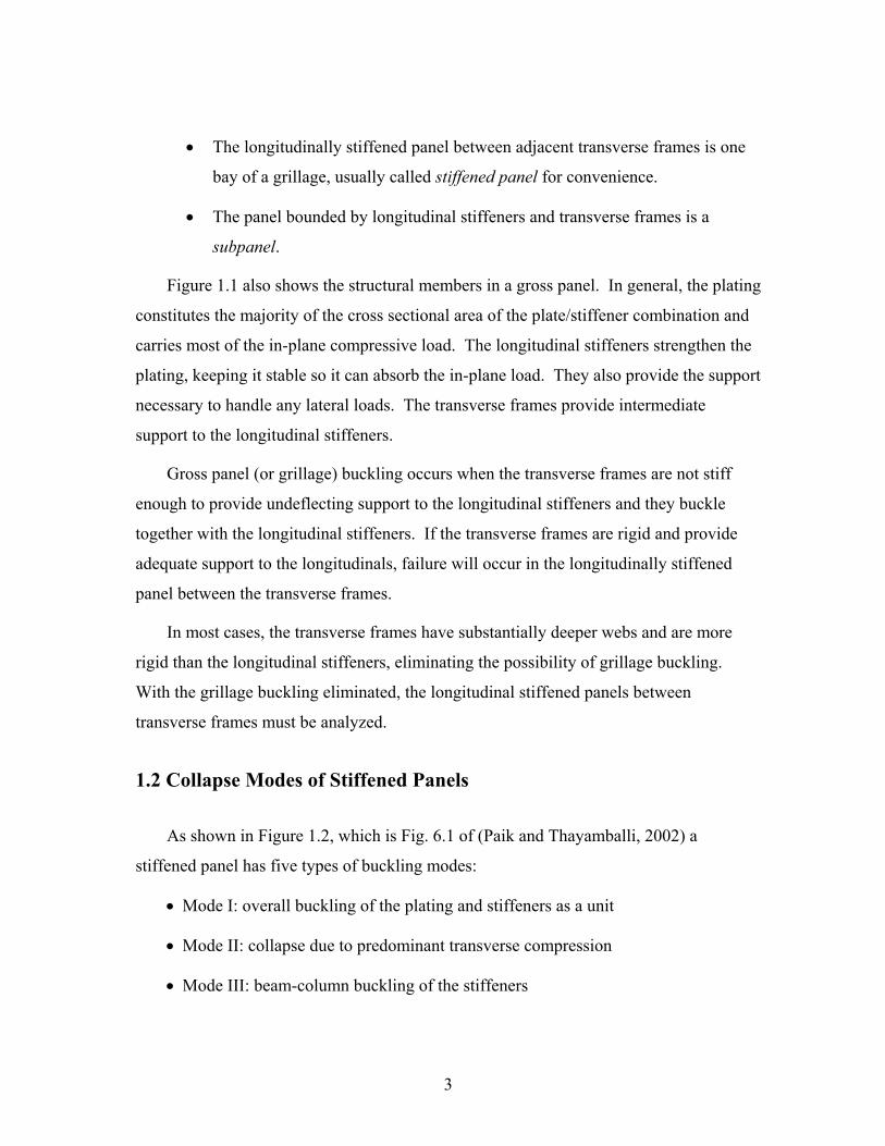
1.2 Collapse Modes of Stiffened Panels
As shown in Figure 1.2, which is Fig. 6.1 of (Paik and Thayamballi, 2002) a
stiffened panel has five types of buckling modes:
• Mode I: overall buckling of the plating and stiffeners as a unit
• Mode II: collapse due to predominant transverse compression
• Mode III: beam-column buckling of the stiffeners

4
• Mode IV: buckling of the stiffener web
• Mode V: flexural-torsional buckling (or “tripping”) of the stiffeners
These modes are neither mutually exclusive nor independent; they can occur together
and they can interact. But they are sufficiently complex that there is no one model or
analysis method that can deal with all of them simultaneously. Instead, it has been found
necessary and useful to make a separate model and a separate ultimate strength analysis
for each of them, because this has allowed expressions to be obtained for the separate
ultimate strengths that are suitable for structural design.
Figure 1.2(a) Overall buckling of the plating and stiffeners as a unit
Figure 1.2(b) Collapse due to predominant transverse compression

5
Figure 1.2(c) Beam-column type collapse, plate induced failure
Figure 1.2(d) Buckling of the stiffener web
Figure 1.2(e) Flexural-torsional buckling (or “tripping”) of the stiffeners

6
The last two buckling modes can be prevented by using stiffeners with good
proportions. The present work deals with the first three modes because they are quite
different and require different (almost opposite) modeling, and yet they can overlap and
interact, and so a more unified approach would be beneficial.
1.3 Two Models for Predicting Ultimate Strength for Modes I and III
Many simplified design methods to estimate the ultimate strength of stiffened steel
panels have been developed, considering one or more of the failure modes among those
mentioned above. Some of those methods have been reviewed by the ISSC technical
committee III.1 on Ultimate Strength (ISSC 2000). Comparisons between some of these
methods have also been made by many researchers (e.g., Das & Garside 1991, Hughes et
al. 1994, ISSC 1994, Rigo et al. 1995, Paik & Kim 1997, Pradillon et al. 2001).
In the Mode I and Mode III ultimate strength analyses of stiffened panels there are two
contrasting models that can be used.
• Beam-column model In this approach the stiffeners are modeled as beam-
columns, characterized mainly by their slenderness ratio λ = L/ρ, with corrections
for the influence of the plating as characterized by the “orthotropic aspect ratio” of
the panel, Πorth, defined in the Nomenclature. A new version of this approach is
presented in Chapter 3.
• Orthotropic plate model In this model large deflection orthotropic plate theory is
used to “smear” the stiffeners into an equivalent orthotropic plate which has an
increased flexural rigidity Dx in the x direction, defined in the Nomenclature. Prof.
Jeom Paik and his colleagues (Paik et al, 2001) have shown that this approach can
be used to predict the ultimate strength of a stiffened panel for the overall collapse
mode (Mode I) under a variety of in-plane loads.
Both models have been used by major societies such as ABS, API, and DnV.
Orthotropic plate method is used in the new Eurocode 3 (Johansson et al, 2001).

7
Currently, DnV is developing a new buckling procedure for stiffened panels using a new
orthotropic model (Steen et al, 2001).
1.3.1 Applications of the Two Models
Beam-column Model
Of its very nature the beam-column model is better when the stiffeners dominate
over the plating; that is, when they act as individual and identical beam-columns, with
little or no interaction. The resulting failure is Mode III. This will occur for:
• a short or wide panel; i.e. small values of L/B
• flexurally strong stiffeners relative to the plating; i.e. small values of D/Dx.
• flexurally strong stiffeners relative to the length; i.e. small values of the
slenderness ratio λ = L/ρ
From the definition of the orthotropic aspect ratio in the Nomenclature we see that
the first two conditions are equivalent to a small value of Πorth. Thus it is possible that
the three conditions are equivalent to a small value of some combination of λ and Πorth,
and Chapter 3 will show that indeed this is the case, and that the appropriate combination
is λΠorth2.
When the stiffeners are dominant (and are properly proportioned so as to prevent
tripping, web bending, web buckling, and other local buckling modes) then the lowest
failure mode is collapse (effectively simultaneous) of the stiffeners as beam-columns. If
there is no pressure the overall beam-column is usually taken as simply supported, but if
there are cross frames then the structure is a multi-span beam-column, and this must be
allowed for in the model. A single span (or one-bay) model is an oversimplification of a
multi-span beam-column, especially if there is pressure.
One of the flanges of the beam-column is the plate flange. Depending on the
direction of the bending in the collapse bay, the collapse will be either “plate-induced” or

8
“stiffener-induced”. In either case the collapse occurs either when the compressed
portion of the cross section loses its axial stiffness, or when the entire section loses its
flexural stiffness. For plate-induced collapse the plating is in compression and it can lose
its axial stiffness due to a combination of plate buckling and membrane yield. For
slender plating they occur in sequence; for more typical ship plating (1.5 < β < 3) they
occur together. For stiffener-induced collapse the portion of the section that is in
compression is not a relatively thin flange (the plating) but rather a relatively deep section
– nearly all of the stiffener. Here the compressed portion loses its axial stiffness
gradually, as yielding occurs progressively, starting at the stiffener flange surface and
extending into the web. Because of the vertical extent of the yielding, it is possible that
the section can lose most of its flexural stiffness before losing its axial stiffness.
Whichever occurs first causes collapse.
Orthotropic plate model
In contrast, it is obvious that the orthotropic plate model is better for small stiffeners.
When the stiffeners are small, the lowest buckling mode is overall or “grillage” buckling.
Until now, it has been customary to only consider the orthotropic model for Mode I
buckling. The beam-column model did not seem to be relevant.
1.4 Properties of the 107 Three-bay Panels
Table 1.1 lists the properties of the 107 three-bay panels that are investigated in this
study. They cover the full range of proportions of typical ship panels. Approximately
half have 3 stiffeners; the others have 5 stiffeners. They are all 3600 mm wide. The first
49 panels (P1-P49) are used in Chapter 2 to verify the accuracy of the improved step-by-
step integration method for inelastic beam-columns. Among the other 58 panels, 55
panels (P50-P107, excluding P57, P66 and P75) are “crossover” panels, as explained in
Section 1.5. All 107 panels are used in Chapter 3 to obtain the formula for applying the
beam-column approach to stiffened panels.
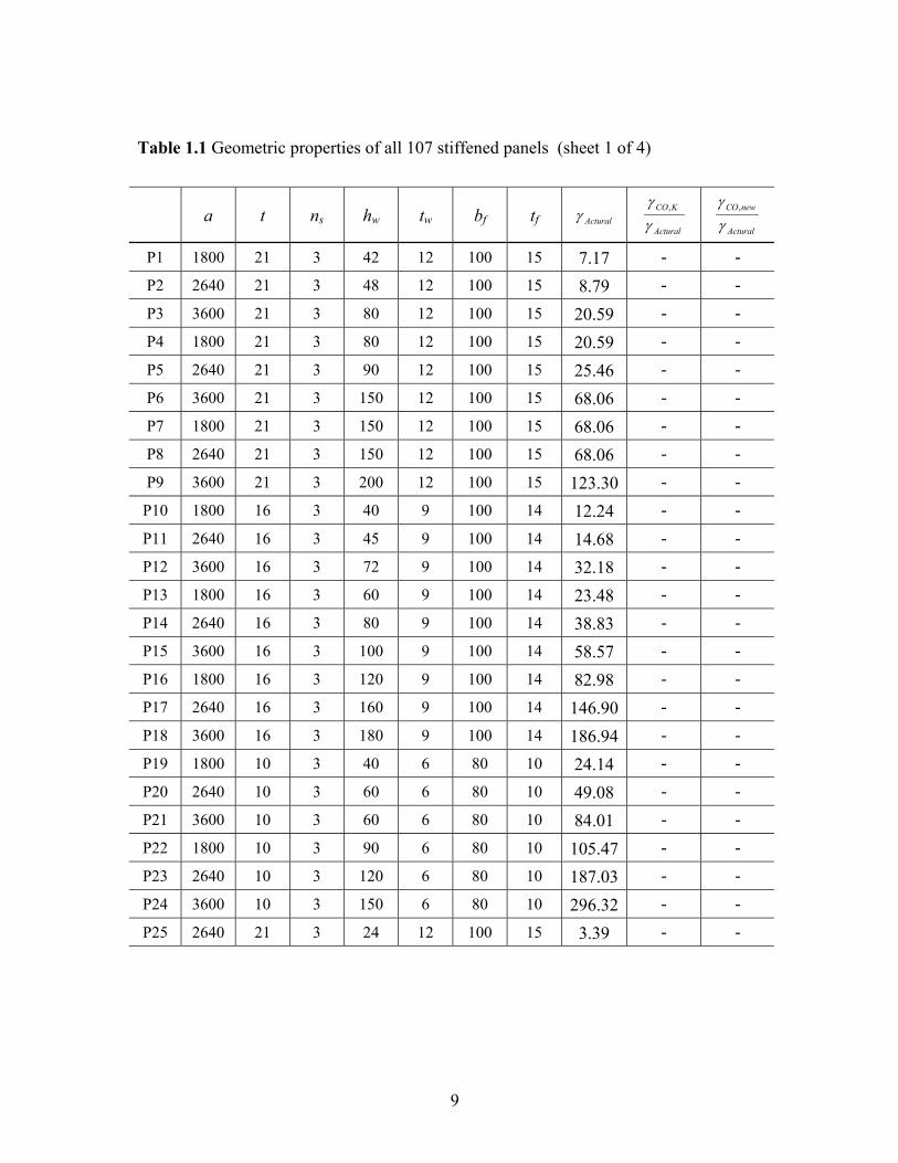
9
Table 1.1 Geometric properties of all 107 stiffened panels (sheet 1 of 4)
a t ns hw tw bf tf Acturalγ
Actural
KCO
γγ ,
Actural
newCO
γγ ,
P1 1800 21 3 42 12 100 15 7.17 - - P2 2640 21 3 48 12 100 15 8.79 - - P3 3600 21 3 80 12 100 15 20.59 - - P4 1800 21 3 80 12 100 15 20.59 - - P5 2640 21 3 90 12 100 15 25.46 - - P6 3600 21 3 150 12 100 15 68.06 - - P7 1800 21 3 150 12 100 15 68.06 - - P8 2640 21 3 150 12 100 15 68.06 - - P9 3600 21 3 200 12 100 15 123.30 - -
P10 1800 16 3 40 9 100 14 12.24 - - P11 2640 16 3 45 9 100 14 14.68 - - P12 3600 16 3 72 9 100 14 32.18 - - P13 1800 16 3 60 9 100 14 23.48 - - P14 2640 16 3 80 9 100 14 38.83 - - P15 3600 16 3 100 9 100 14 58.57 - - P16 1800 16 3 120 9 100 14 82.98 - - P17 2640 16 3 160 9 100 14 146.90 - - P18 3600 16 3 180 9 100 14 186.94 - - P19 1800 10 3 40 6 80 10 24.14 - - P20 2640 10 3 60 6 80 10 49.08 - - P21 3600 10 3 60 6 80 10 84.01 - - P22 1800 10 3 90 6 80 10 105.47 - - P23 2640 10 3 120 6 80 10 187.03 - - P24 3600 10 3 150 6 80 10 296.32 - - P25 2640 21 3 24 12 100 15 3.39 - -

10
Table 1.1 Geometric properties of all 107 stiffened panels (sheet 2 of 4)
a t ns hw tw bf tf Acturalγ
Actural
KCO
γγ ,
Actural
newCO
γγ ,
P26 1800 21 5 42 12 100 15 10.31 - - P27 2640 21 5 48 12 100 15 12.62 - - P28 3600 21 5 80 12 100 15 29.44 - - P29 1800 21 5 80 12 100 15 29.44 - - P30 2640 21 5 90 12 100 15 36.35 - - P31 3600 21 5 150 12 100 15 96.39 - - P32 1800 21 5 150 12 100 15 96.39 - - P33 2640 21 5 150 12 100 15 96.39 - - P34 3600 21 5 200 12 100 15 173.55 - - P35 1800 16 5 40 9 100 14 17.48 - - P36 2640 16 5 45 9 100 14 20.95 - - P37 3600 16 5 72 9 100 14 45.77 - - P38 1800 16 5 60 9 100 14 33.45 - - P39 2640 16 5 80 9 100 14 55.17 - - P40 3600 16 5 100 9 100 14 83.00 - - P41 1800 16 5 120 9 100 14 117.30 - - P42 2640 16 5 160 9 100 14 206.66 - - P43 3600 16 5 180 9 100 14 262.39 - - P44 1800 10 5 40 6 80 10 34.57 - - P45 2640 10 5 60 6 80 10 70.08 - - P46 3600 10 5 80 6 80 10 119.62 - - P47 1800 10 5 90 6 80 10 149.97 - - P48 2640 10 5 120 6 80 10 264.85 - - P49 3600 10 5 150 6 80 10 417.97 - -

11
Table 1.1 Geometric properties of all 107 stiffened panels (sheet 3 of 4)
a t ns hw tw bf tf Acturalγ
Actural
KCO
γγ ,
Actural
newCO
γγ ,
P50 1800 21 3 50 20 200 30 35.12 0.64 0.93 P51 1800 21 3 84 12 100 15 22.47 0.84 0.90 P52 1800 21 3 50 10 200 30 34.57 0.64 0.93 P53 1800 16 3 36 20 200 30 44.60 0.54 0.88 P54 1800 16 3 56 12 100 15 23.03 0.83 0.88 P55 1800 16 3 81 5 60 10 18.14 0.98 1.04 P56 1800 16 3 31 10 200 30 36.92 0.64 1.12 P57 2640 21 3 60 12 100 15 12.56 - - P58 1800 10 3 28 12 100 15 26.97 0.74 0.89 P59 1800 10 3 41 5 60 10 19.50 0.93 0.94 P60 2640 21 3 80 20 200 30 69.83 0.69 0.94 P61 2640 21 3 123 12 100 15 45.92 0.87 0.93 P62 2640 21 3 75 10 200 30 61.74 0.75 0.98 P63 2640 16 3 58 20 200 30 85.10 0.60 0.95 P64 2640 16 3 84 12 100 15 46.88 0.86 0.92 P65 2640 16 3 53 10 200 30 73.60 0.68 1.02 P66 2640 21 3 95 12 100 15 83.63 - - P67 2640 10 3 45 12 100 15 56.01 0.75 0.92 P68 2640 10 3 62 5 60 10 40.62 0.93 0.96 P69 3600 21 3 112 20 200 30 120.85 0.75 0.99 P70 3600 21 3 166 12 100 15 83.65 0.89 0.94 P71 3600 21 3 106 10 200 30 106.72 0.81 0.98 P72 3600 16 3 83 20 200 30 147.74 0.65 1.01 P73 3600 16 3 120 12 100 15 92.23 0.82 0.88 P74 3600 16 3 76 10 200 30 125.70 0.73 1.03 P75 2640 21 3 150 12 100 15 68.06 - - P76 3600 10 3 65 12 100 15 105.18 0.75 0.92 P77 3600 10 3 86 5 60 10 75.71 0.92 0.95 P78 1800 21 5 84 20 200 30 100.22 0.58 0.91

12
Table 1.1 Geometric properties of all 107 stiffened panels (sheet 4 of 4)
a t ns hw tw bf tf Acturalγ
Actural
KCO
γγ ,
Actural
newCO
γγ ,
P79 1800 21 5 116 12 100 15 58.32 0.77 0.87 P80 1800 21 5 93 10 160 20 68.53 0.71 0.89 P81 1800 21 5 77 10 200 30 85.73 0.65 1.01 P82 1800 16 5 60 20 200 30 116.54 0.55 0.96 P83 1800 16 5 82 12 100 15 63.34 0.73 0.81 P84 1800 16 5 54 10 200 30 98.64 0.62 1.12 P85 1800 10 5 31 20 200 30 144.46 0.53 0.95 P86 1800 10 5 45 12 100 15 77.64 0.63 0.83 P87 1800 10 5 56 5 60 10 48.66 0.86 0.91 P88 2640 21 5 126 20 200 30 195.96 0.66 0.96 P89 2640 21 5 168 12 100 15 121.14 0.82 0.90 P90 2640 21 5 136 10 160 20 133.62 0.79 0.93 P91 2640 21 5 116 10 200 30 165.09 0.73 0.98 P92 2640 16 5 93 20 200 30 231.35 0.61 1.02 P93 2640 16 5 120 12 100 15 129.47 0.78 0.86 P94 2640 16 5 82 10 200 30 184.73 0.72 1.11 P95 2640 10 5 52 20 200 30 291.22 0.58 1.01 P96 2640 10 5 68 12 100 15 157.36 0.68 0.90 P97 2640 10 5 84 5 60 10 103.97 0.87 0.91 P98 3600 21 5 174 20 200 30 347.81 0.72 0.99 P99 3600 21 5 223 12 100 15 218.23 0.87 0.94 P100 3600 21 5 185 10 160 20 236.74 0.84 0.96 P101 3600 21 5 159 10 200 30 283.85 0.81 1.00 P102 3600 16 5 131 20 200 30 415.25 0.65 1.07 P103 3600 16 5 164 12 100 15 241.07 0.81 0.88 P104 3600 16 5 133 10 160 20 262.01 0.80 0.93 P105 3600 16 5 115 10 200 30 321.76 0.78 1.10 P106 3600 10 5 76 20 200 30 524.44 0.62 1.06 P107 3600 10 5 95 12 100 15 291.10 0.71 0.94

13
1.5 Flexural Rigidity Ratio for Simultaneous Buckling
Figure 1.3 is a simplified design space with only two design variables – plate
thickness and stiffener height. The axis normal to the page is the weight of the stiffened
panel, and the contours are those of constant weight. The figure shows the constraint
against local plate buckling and the constraint against overall panel buckling, and it is
evident that the optimum design is at the junction of the two constraints
Figure 1.3 Design space for optimum design of a stiffened panel
It is useful to have a structural parameter by which one can determine which mode of
buckling occurs first. The following flexural rigidity ratio is commonly used for this
purpose:
DbEI x=γ (1.1)
Plate buckling
tp1
final tp
hs hs1final hs
tp

14
It is tempting to use the condition of simultaneous buckling as a simple way of
obtain a least weight panel. But from (Tvergaard and Needleman, 1975) and other
studies it has long been known that, for elastic buckling, a simultaneous occurrence of the
two modes causes the curve of load vs. average axial strain to have a much steeper
negative slope immediately after buckling, compared to the post-buckling slope for
overall buckling when plate buckling is not simultaneous, either occurring beforehand or
not at all. In other words, for “crossover” panels, for which γ is at or near the elastic
“crossover” value, the load shedding is both sudden and large scale. Perhaps not aware of
this earlier work (Grondin et al, 2002) have reported this same result.
For panels that buckle elastically, either because they are very slender or are made of
composite materials, designers generally prefer that local plate buckling should occur
first, thereby giving some warning about possible overall buckling, which is more
extensive and therefore more serious.
(Klitchieff, 1951) derived a formula for the “crossover” value of γ, beyond which the
stiffeners are large enough that local plate buckling precedes overall buckling.
++=tB
ACB
aN SsKCO
2,
4)1( ξπ
ξγ (1.2)
where: 2
2 4
=
baξ
and
1cos
/1
cosh
/1
sinh
11
1cos
/1
cos
/1
sin
11
+−
+
+
++
+−
−
−
−−=
ss Nba
ba
Nba
baCππ
ξ
πξ
ξππξ
πξ
ξ
In order to access the accuracy of Eq.(1.2) (Hughes and Ghosh, 2003) performed
repeated eigenvalue analyses for 55 panels, gradually adjusting the stiffener height until

15
the local plate buckling stress and the overall (interframe) buckling stress were
approximately equal (usually within 10%). In Table 1.1 these “crossover” panels are
P50-P107 (excluding P57, P66 and P75). Besides the structural dimensions, the table
gives the value of Actualγ (which is also ActualCO,γ for the “crossover” panels as obtained
from eigenvalue analyses), and the ratio of the Klitchieff value KCO,γ to ActualCO,γ . The
average error (using absolute values) of the ActualCO
KCO
,
,γ
γ ratio is 26 % and the COV is
0.148.
This is a relatively large error, and so Hughes and Ghosh derived a new expression
for the crossover value of γ. They included allowance for the rotational restraint of
stiffeners developed by (Paik and Thayamballi, 2000) an allowance for web bending and
an allowance for transverse shear in the stiffener web. The result is the following simpler
and much more accurate formula (7 % mean error, COV 0.073):
Π+Π+
+
=
21 423
2
orthorthETw
w
CrTCO
AGAGA
ktb
Aa
ησ
γ (1.3)
where:
CrCrCrCrk ζζζ 565.3974.1396.04 23 +−+= for 20 <≤ Crζ
4.0881.0951.6−
−=Cr
Crkζ
for 202 <≤ Crζ
025.7=Crk for 20≥Crζ
and

16
ζζ rCr C= where
bd
tt
C
w
r 3
6.31
1
+
=
The last column of Table 1.1 shows the ratio of the NewCO,γ given by eq. (1.3) relative
to the actual value. The average error (using absolute values) of ActualCO
NewCO
,
,γ
γ is 7 %
(with COV of 0.073), compared to 26 % (with COV of 0.148) for the Klitchieff formula,
Eq. (1.2). Thus the new formula for crossover panels which are P50-P107 (excluding
P57, P66 and P75) is more accurate and yet simpler in format.
1.6 Significance of “Crossover” Proportions in Typical Ship Panels
The undesirable post-bucking behavior of elastic “crossover” panels raises the
question as to whether the same behavior occurs for panels that buckle inelastically. This
is important for ship panels, in which typically both buckling modes are inelastic. To
answer this question, the ship structures research group at Virginia Tech has performed
an extensive series of nonlinear finite element ultimate strength calculations, using
ABAQUS, on 107 stiffened panels. Approximately half (55) of the panels were
“crossover” panels, which means that their value of γ is equal or very close to the
crossover value given by Eq. (1.3), regardless of whether their elastic buckling stresses
(local and overall) are above or below the yield stress. The results are presented in
Chapter 4. All of these panels are typical ship panels, for which extensive yielding occurs
along with the buckling, with a strong two-way interaction. Because of these inelastic
complications, the “crossover” panels did not have less ultimate strength but some of
them (14 in all) did exhibit steep load shedding. Also, this study revealed that some
“crossover” panels (21 out of 55) do have one surprising feature - they cannot be
adequately modeled by orthotropic-based methods, whereas all of them can be modeled
adequately by a beam-column approach.

17
1.7 Ultimate Strength of a Subpanel
The collapse of stiffened panels under transverse compression with or without
pressure is due to a localized buckling of subpanels, which is Mode II shown in Fig.
1.2(b).
For transverse compression of these subpanels (Valsgård, 1979) presented a method
for estimating the ultimate strength of a wide plate. However, Valsgård’s method was for
wide plates that are simply supported on all four edges. For stiffened panels subjected to
a lateral pressure the edge condition is in between simply supported and clamped, and
until now no method was available that could deal with this.
In Chapter 5 a direct numerical method is presented in which the edge restraint
problem is solved by applying end moments at the loaded edges. The magnitude of the
end moments depends on the plate slenderness and the magnitude of the initial deflection.
The new method gives results that agree well with nonlinear FE results.
1.8 Summary
This chapter mainly states the motivation of this research. The work presented in the
following chapters includes four parts, which can be summarized as follows:
• Chapter 2 derives an improved step-by-step numerical integration procedure based
on (Chen and Liu, 1987) to calculate the ultimate strength of a beam-column under
axial compression, end moments, and lateral loads. A special procedure is
developed to analyze the collapse of a three-span beam-column which represents a
typical stiffener-plate combination in a three-bay stiffened panel.
• Chapter 3 compares the results of the fine mesh elasto-plastic finite element
ultimate strength analyses with the results of the continuous beam-column
calculations for the stiffener-induced collapse of 107 three-bay stiffened panels,
covering a wide range of panel length, plate thickness, and stiffener sizes and
18
proportions. It shows that the three span beam-column model developed in Chapter
2 gives good results for stiffener-induced failure when the orthotropic plate
parameter Πorth is small. Section 3.2 shows that the three span beam-column model
is sufficiently general to apply to any panel with three or more spans. Sections 3.3
and 3.4 then use the FE results to obtain a simple formula that corrects the beam-
column result and gives good agreement for panel ultimate strength for all of the
107 panels. The formula is extremely simple, involving only one parameter: the
product λΠorth2.
• Chapter 4 compares the predictions of the new beam-column formula and the
orthotropic plate theory with the FE solutions for all 107 panels. It shows that the
orthotropic plate theory cannot model the “crossover” panels adequately, whereas
the beam-column method can predict the ultimate strength well for all of the 107
panels, including the “crossover” panels. A brief discussion about possible cause
of the large overestimate of ultimate strength finishes this chapter.
• Chapter 5 presents a new numerical method for calculating the ultimate strength of
stiffened panels under transverse compression with and without pressure. The
method is based on a further extension of the nonlinear beam-column theory
presented in Chapter 2, and application of it to a continuous plate strip model to
calculate the ultimate strength of subpanels. This method is shown to agree well
with nonlinear FE solutions.
19
Chapter 2
Inelastic Beam-Columns
2.1 Introduction
The critical load of a geometrically perfect beam-column is usually determined by
the eigenvalue (or bifurcation) approach. The lateral deflection will not occur until the
applied load reaches a critical value. At this critical load, a small disturbance on the
member will produce a large lateral deflection. To obtain the critical load, a linear
differential equation is first written down for the member in a slightly deformed state.
The solution to the characteristic equation derived from this governing differential
equation then gives the critical load of the member. This approach is also known as the
method of neutral equilibrium.
To account for the inelasticity in the eigenvalue analysis, the concept of effective
modulus (tangent modulus and reduced modulus) is widely used. Since the effect of
inelasticity is to reduce the stiffness of the member, the plastic buckling load in an
inelastic analysis is always smaller than that of the elastic bucking analysis.
If the member is geometrically imperfect, lateral deflection will begin as soon as the
load is applied. As a result, the above neutral equilibrium method cannot be applied for
the case of an imperfect member. Instead, a more complex analysis known as the load-
deflection approach must be used. In this approach, the complete load-deflection
response of the member is traced from the start of loading up to the critical load.
Rigorous load-deflection analysis for inelastic, imperfect members is rather complicated.

20
Numerical or approximate methods (Chen and Atsuta, 1976, 1977) therefore play an
important role in the solution for the critical loads, and recourse is made to techniques
such as the Raleigh-Ritz method, Galerkin’s method, Newmark’s method, and the step-
by-step method.
This chapter presents a numerical integration procedure based on the step-by-step
method, known herein as the ‘modified step-by-step method’. The method is applicable
to imperfect beam-columns with geometric and material nonlinearities. Several beam-
columns with different cross sections, different load conditions, and different boundary
conditions are analyzed by the method, and the results are shown to be very accurate by
comparing them with fine mesh finite element (FE) solutions.
2.2 Assumptions
The three basic assumptions used in the following derivation are:
1. The cross section remains plane after bending, and remains undeformed in the
cross section plane.
2. The stress-strain relationship is assumed to be elastic-perfectly plastic. (Fig. 2.1)
3. The initially imperfection shape of the pinned-pinned member follows a half-sine
wave; the initial imperfection shape of the clamped-clamped member follows a
cosine wave.
Also, the beam-column is assumed to be symmetric about the mid-length cross
section.

21
Figure 2.1 Idealized stress-strain diagram
2.3 M - F - P relationship
In the process of numerical integration, we will need to use the nonlinear relationship
between the internal moment M and the curvature F and the axial force P. To derive the
M- F -P relationship, we need to evaluate the integrals for the axial net force P and
internal bending moment M. The force equilibrium condition and moment equilibrium
condition determine the strain or stress distribution, from which we can get the
expression for curvature F in terms of P and M.
2.3.1 Rectangular cross section
When a member with rectangular cross section (h X b) is subjected to axial
compression, a plastic collapse mechanism will form as sketched in Fig. 2.2. Before the
formation of the final perfect plastic hinge (Fig. 2.2d), the cross section will experience
three stages: elastic (no yielding, Fig. 2.2a), primary plastic (Fig. 2.2b), and secondary
plastic (Fig. 2.2c).
E
s
e
sY
eY 0

22
Strain Stress
Figure 2.2 Strain and stress diagram (Rectangular section)
M
eU ≤ eY sU ≤ sY AP
a =σ
=
eL > -eY sL > -sY
Center line +
(a) Elastic
h
sa
eY M
eU > eY sU = sY
=
eL ¥ -eY sL ¥ -sY
Center line +
(b) Primary plastic
sa
eY M
eU > eY sU = sY
=
eL < -eY sL = -sY
Center line +
(c) Secondary plastic
-eY
sL = -sY
(d) Perfect plastic hinge
sU = sY
dPH
dSP
dSPD
dPP

23
Elastic, Fig. 2.2(a)
Since the member remains fully elastic, the moment-curvature relationship has the
simple form
MEI
=Φ (2.1)
Primary plastic, Fig. 2.2(b)
Equilibrium:
The axial force P and the internal moment M are related to the stress s(z) by
dAPA∫= σ
dzybzbd PPh
h
d
PPY ∫−
−+= 2
2
)(σσ (2.2)
dAzMA∫= σ
dzbzzdh
bd PPh
h
dfPPY ∫
−
−+
−= 2
2
)(2
σσ (2.3)
where:
LPP
LY hzdh
z σσσ
σ +
+
−−
=2
)( (2.4)
Substitute Eq. 2.4 into Eq. 2.2, solve for sL, the substitute sL and s(z) into Eq. 2.3
and solve for dPP.
Finally, get curvature
)( PP
LY
PP
LY
dhEdh −−
=−−
=Φσσεε (2.5)
Secondary plastic, Fig. 2-2(c)
Equilibrium:

24
The axial force P and the internal moment M are related to the stress s(z) by
dAPA∫= σ
dzbzddb SPh
hSPD
d
dSPDSPY ∫−
−+−= 2
2
)()( σσ (2.6)
dAzMA∫= σ
dzbzzdhbddhbd SPh
hSPD
d
dSPD
SPDYSP
SPY ∫−
−+
−+
−= 2
2
)(22
σσσ (2.7)
where:
YSPDSPDSP
Y dhzddh
z σσ
σ −
−+
−−=
22)( (2.8)
Substitute Eq. 2.8 into Eq. 2.6, solve for dSPD, the substitute dSPD and s(z) into Eq.
2.7 and solve for dSP.
Finally, get curvature
)(22
SPDSP
Y
SPDSP
Y
ddhEddh −−=
−−=Φ
σε (2.9)
Perfect plastic hinge, Fig. 2-2(d)
From equilibrium:
( )hdbP PHY −= 2σ (2.10)
Get:
Y
Y
PH
hbhP
dσ
σ
2
+
= (2.11)
The perfect plastic hinge moment MPH then is:
)( PHPHY dhbdM −= σ (2.12)

25
Note that if the member is fully elastic, the axial force has no effect on the moment-
curvature relationship. However, as soon as yielding commences, M and F are affected
by the axial force.
Figure 2.3 Cross-sectional geometry (Asymmetric I)
2.3.2 Asymmetric I cross section
Figure 2.3 shows the cross section geometry properties of a T type stiffener with
attached plating (acting as the bottom flange), representing an asymmetric I cross section,
which is of the most interest in this thesis.
Figure 2.4 shows a series of strain and stress diagrams that correspond to four stages
of loading sequences: no yielding, yielding in flange, yielding in web, and yielding in
plating, respectively. For convenience, they are designated in the following as Case 1,
Case 2, Case 3, and Case 4.
Note that Case 2 - 4 are all primary plastic. For the sake of simplicity, the secondary
plastic cases (yielding in tension starting from the bottom of the plating) are not covered
here for asymmetric I cross section.
bf
tf
twhw
b
t z0
Centroidal axis
hT =tf + hw + t
Stiffener flange (bf x tf)Stiffener web (hw x tw)
Plating (b x t)

26
Case 1: Elastic, Fig. 2.4(a)
Since the member remains fully elastic, the moment-curvature relationship has the
same form as Eq. 2.1 for rectangular section.
Case 2: Yielding in flange, Fig. 2.4(b)
Equilibrium:
The axial force P and the internal moment M are related to the stress s by
dAPA∫= σ
dzbzdztzdzbzdbzt
z
zht
zt w
dzh
zht fffYwfT
w∫∫∫
−
−
−+
−
−−
−++++= 0
0
0
0
0
0
)()()( σσσσ (2.13)
dAzMA∫= σ
dzbzzdzztzdzzbzd
zhdbzt
z
zht
zt w
dzh
zht ff
TffYwfT
w∫∫∫
−
−
−+
−
−−
−++++−−= 0
0
0
0
0
0
)()()()2
( 0 σσσσ
(2.14)
where:
LfT
LY zzdh
z σσσσ ++−−
= )()( 0 (2.15)
Substitute Eq. 2.15 into Eq. 2.13, solve for sL, the substitute sL and s(z) into Eq.
2.14 and solve for df .
Finally, get curvature
)( fT
LY
fT
LY
dhEdh −−
=−−
=Φσσεε (2.16)

27
Figure 2.4 Strain and stress diagram for asymmetric I cross section (Case 1 and 2)
M
Strain Stress
eU ≤ eY sU ≤ sY AP
a =σ
=
eL < eY sL < sY
Centroidal Axis
+
(a) CASE 1, elastic
hT
tf
tp
eU > eY sU = sY sa
M
=
eL < eY sL < sY
Centroidal Axis
+
(b) CASE 2, yielding in flange
eY df
Strain Stress

28
Figure 2.4 Strain and stress diagram for asymmetric I cross section (Case 3 and 4)
Strain Stress
(c) CASE 3, yielding in web
(d) CASE 4, yielding in plating
Strain Stress
eU > eY sU = sY sa M
=
eL < eY sL < sY
Centroidal Axis
+eY dw
eU > eY sU = sY sa
=
eL < eY sL < sY
Centroidal Axis
+
eY
dp
tp
M

29
Case 3: Yielding in web, Fig. 2-4(c)
Equilibrium:
The axial force P and the internal moment M are related to the stress s by
dAPA∫= σ
dzbzdztzdttbzt
z
zdht
zt wwwYffYww
∫∫−
−
−−+
−+++= 0
0
0
0
)()( σσσσ (2.17)
dAzMA∫= σ
dzbzzdzztzdzthdtt
zhtbzt
z
zdht
zt ww
fTwwYf
TffYww
∫∫−
−
−−+
−++−−−+−−= 0
0
0
0
)()()2
()2
( 00 σσσσ
(2.18)
where:
LwfT
LY zzdth
z σσσσ ++−−
−= )()( 0 (2.19)
Substitute Eq. 2.19 into Eq. 2.17, solve for sL, the substitute sL and s(z) into Eq.
2.18 and solve for dw .
Finally, get curvature
)( wfT
LY
wfT
LY
dthEdth −−−
=−−
−=Φ
σσεε (2.20)
Case 4: Yielding in plating, Fig. 2-4(d)
Equilibrium:
The axial force P and the internal moment M are related to the stress s by
dAPA∫= σ

30
dzbzbdhttbzd
zpYwwYffYp
∫−
−+++= 0
0
)(σσσσ (2.21)
dAzMA∫= σ
dzbzzd
ztbdhzthtt
zhtbzd
z
ppY
wwwY
fTffY
p
∫−
−+−−++−+−−= 0
0
)()2
()2
()2
( 000 σσσσ
(2.22)
where:
Lp
LY zzdt
z σσσσ ++−−
= )()( 0 (2.23)
Substitute Eq. 2-23 into Eq. 2-21, solve for sL, the substitute sL and s(z) into Eq. 2-
22 and solve for dp .
Finally, get curvature
)( p
LY
p
LY
dtEdt −−
=−−
=Φσσεε
(2.24)
The moment-curvature-thrust relations developed above are for stiffeners with
rectangular flanges. For stiffeners with bulb and other cross sections with general stress-
strain behavior, the derivations are similar.

31
2.4 Modified Step-by-step Method
In the original step-by-step method (Chen and Liu, 1987):
1. The member is divided into n segments with n + 1 stations within the full length.
2. The deflection of the first station is specified.
3. The deflections at subsequent stations are calculated from station to station in a
systematic, forward marching manner.
4. The applied force corresponding to the specified deflection is sought iteratively.
5. Stop the iteration when the deflection at the other end equals to zero.
This procedure, which is discussed in more detail in Chen and Liu’s book, can only
deal with pinned-pinned boundary conditions. In the following sections, the method is
modified so that it is applicable for both pinned-pinned and clamped boundary condition.
A special procedure for three-span beam-columns is also developed.
2.4.1 Pinned-pinned
Consider Figure 2.5, in which a pinned-pinned beam-column with initial deflection
of w0 is shown. The member is subjected to axial compression load. The boundary
conditions are:
w = w’’ = 0 at 2ax ±= (2.25)
Because of symmetry, only half of the overall length of the beam-column needs to be
analyzed. Using the second-order central difference equation for the curvature at station
1, we can get the deflection at station 2:
121
2 2wxw +∆
Φ−= (2.26)

32
Figure 2.5 Geometry for step-by-step procedure (Pinned-pinned member)
For a given w1, the maximum added displacement (at the middle), we can use the
following step-by-step numerical integration procedure to find the corresponding axial
load P:
1. Set initial value for P
2. Calculate the external moment at station 1:
Mext1 = P (w1 + w01) (2.27)
3. From Mint1 = Mext1, obtain the curvature F1 from the moment-curvature-thrust
relationship developed in Section 2.3.
4. Calculate the deflection of Station 2, w2, from Eq. 2.26.
5. Knowing w2, calculate the external moment at station 2:
Mext2 = P (w2 + w02) (2.28)
6. From Mint2 = Mext2, obtain F2 from the moment-curvature-thrust relationship
developed in Section 2.3.
w01= w0 ,
w1 w2 w3 … … wn
Station: 1 2 3 … … n
P P
w0n= w0 axπcos
z x
a
Deflected shape

33
7. The deflection at Station 3 is obtained from the second order difference equation,
1222
3 22
wwxw −+∆Φ
−= (2.29)
8. Repeat Steps 5, 6 and 7 for successive stations until the end of the member is
reached.
If the displacement wn at the end of the member differs from zero, a correction needs
to be made to P, then repeat the whole procedure until wn equals zero.
Figure 2.6 Clamped-clamped member
2.4.2 Clamped-clamped
Consider Figure 2.6, in which a clamped-clamped member with initial deflection of
w0 is shown. The member is subjected to axial compression load. The boundary
conditions are:
w01= w0 ,
w1 w2 w3 … … wn
Station: 1 2 3 … … n
P
M0 ME
P
w0n= ( )axw π2
2 cos10 +
z x
a
Deflected shape
34
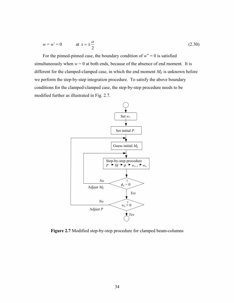
w = w’ = 0 at 2ax ±= (2.30)
For the pinned-pinned case, the boundary condition of w’’ = 0 is satisfied
simultaneously when w = 0 at both ends, because of the absence of end moment. It is
different for the clamped-clamped case, in which the end moment ME is unknown before
we perform the step-by-step integration procedure. To satisfy the above boundary
conditions for the clamped-clamped case, the step-by-step procedure needs to be
modified further as illustrated in Fig. 2.7.
Figure 2.7 Modified step-by-step procedure for clamped beam-columns
wn = 0
Set w1
?
No fn = 0
?
Set initial P
Guess initial ME
Step-by-step procedure P M f wi+1 wn
Adjust ME Yes
No
Yes Adjust P

35
Figure 2.8 A stiffener-plate combination as in a 3 bay stiffened panel
Figure 2.9 The free body diagram of the stiffener-plate
2.4.3 Three-span simply supported beam-columns
Consider an equally spaced three-span simply supported member subjected to axial
compressive load as shown in Fig. 2.8. Assume the initial deflection shape follows an
up-and-down half sine pattern. If the cross section is symmetric about the x-axis
(rectangular and symmetric I sections, for example), each bay will behave just as a
separate pinned-pinned member. If the cross section is not symmetric about the x-axis
(asymmetric I section, for example), there will be reactionary bending moments MR at
mid-supports once the member is deflected, as shown in Fig. 2.9. With the following
P P
MR
qend = qmid
(b) The end bay
P
MRqmid
P
M
(a) The middle bay (Half)
w1
wn
x
x z
P
w0
A
A
P
A - A
a a a

36
special case, another procedure is developed to deal with the unknown bending moment
MR.
Figure 2.10 Modified step-by-step procedure for a three-span beam-column
Consider Figure 2.8 in which the initially crooked beam-column represents a
stiffener with attached plating in a 3 bay stiffened panel. Figure 2.9 shows the free body
diagram of the stiffener-plating combination. Fig. 2.9a represents half of the middle bay,
in which stiffener-induced failure will occur; Fig. 2.9b represents the end bay, which will
remain elastic.
For an initially crooked simply supported beam-column with elastic behavior, like
the end bay, the analytical load-deflection equation is:
Set w1
?
No wn = 0
?
Set initial P
Guess initial MR
Step-by-step procedure P M f wi+1 wn
Adjust MR
Yes
Yes Adjust P
'nw = qend No

37
axw
ax
kakxkx
EIkMxw R πφ sin)1
tansin(cos)( 02 +−+−= (2.31)
where:
EPP
−=
1
1φ
(2.32)
EIPk = (2.33)
The first derivative of w(x) gives the slope, at the connection between middle bay
and end bay
aw
akak
EIkM
w Rend
πφθ 0
2
1tan
)0(' +
+−== (2.34)
At the connection between the end bay and the middle bay, we have two boundary
conditions for the middle bay:
w = 0 at 2ax = (2.35)
w’ = qend at 2ax = (2.36)
With these two boundary conditions, the procedure presented in Fig. 2.10 can be
used to find the solution for axial force P corresponding to a specified deflection w1.

38
2.4.4 Under combined axial compression and uniform lateral load
For a uniform lateral load q, the moment equilibrium equations for a member under
combined axial compression and uniform lateral load become
[ ]22
0, )1(28
)( xiqqaMwwPM Eiiiext ∆−−+−+= (2.37)
where i is the station number, and ∆x is the station length.
For the pinned-pinned case, ME is the applied bending moment at the end, if it exists.
For the clamped-clamped case, ME is the end moment which satisfies the boundary
conditions.
2.5 Verification of the Modified Step-by-step Method
2.5.1 General
The modified step-by-step numerical integration procedure can be used to determine
the equilibrium configuration of beam-columns. By changing the value of maximum
deflection (w1) and repeating the procedure, a load-deflection curve can be generated.
Such a curve is shown in Fig. 2.11. The peak point represents the ultimate strength.
Note that both the ascending and descending branches of the load-deflection curve can be
traced using this procedure. Thus, a complete load-deflection analysis can be performed.

39
Figure 2.11 Load-deflection behavior of a beam-column
A FORTRAN program called ULTBEAM, is developed based on the modified step-
by-step method. Using ULTBEAM, the following four classes of problems are studied:
1. Single span simply supported beam-column under axial compression
2. Single span clamped beam-column under axial compression
3. Single span clamped beam-column under combined axial compression and
uniform lateral load
4. Three span beam-column under axial compression
In each case a fine mesh finite element analysis using ABAQUS is also performed
for verification. The 2-node linear beam elements (B21) are used. The mesh is 80
elements per span length.
2.5.2 Single span pinned-pinned beam-column under axial compression
The procedure developed in Section 2.4.1 can be applied directly for this case. To
get the load-deflection path, we set a series of values of the displacement at the middle of
P
w1 (wmax) 0
(Pult, wult)

40
the member, and get the corresponding axial forces using the step-by-step procedure.
The peak value of the axial forces is the ultimate load Pult.
Consider two single span beam-columns (SC1 and SC2) with asymmetric I cross-
section. Table 2.1 shows the dimensions.
Table 2.1 Geometric properties one-span stiffener-plate combinations in DW5120 and Smith3b (mm)
a b t hw tw bf tf w0
SC1 5120 910 20 598.5 12 200 20 5.12
SC2 1524 304.8 6.4 64.25 4.65 27.94 6.35 2.9
Material properties:
SC1: sY = 315.0 MPa, E = 208000, n = 0.3
SC2: sY = 247.3 MPa, E = 205800, n = 0.3
Calculations are made for two different initial deflection cases: one is with the
downward initial deflection (toward the plate side, which causes the stiffener-induced
failure), and the other one is with the upward initial deflection (toward the stiffener side,
which causes the plate-induced failure). The ultimate loads for both the stiffener-induced
failure and the plate-induced failure are listed in Table 2.2.
Table 2.2 Ultimate loads for stiffener-induced and plate-induced failure modes
Stiffener-induced Plate-induced sult (MPa) ULTBEAM ABAQUS ULTBEAM ABAQUS
SC1 304.1 303.6 310.8 310.8
SC2 167.4 158.0 226.3 219.6

41
0 0.4 0.8 1.2
0
0.2
0.4
0.6
0.8
1
ULTBEAMABAQUS
wmax
LX 1000
PPY
Figure 2.12 Load-deflection curve, stiffener-induced failure, SC1
0 1280 2560 3840 5120
-0.8
-0.6
-0.4
-0.2
0
ULTBEAMABAQUS
L
w
Figure 2.13 Added deflection under ultimate load, stiffener-induced failure, SC1
sult = 304 MPa
ssY

42
From the above comparison, we see that the modified step-by-step procedure
(ULTBEAM) gives very accurate prediction of the ultimate strength of a simply
supported beam-column under axial compression. We also observe that simply supported
members with stiffener-induced failure modes are weaker than those with plate-induced
failure modes. This is true for all of the single stiffener beam-columns in this chapter and
for all of the 107 three-bay panels in Chapter 4.
The load-deflection curve for SC1 with downward initial deflection is shown in Fig.
2.12, in which the equilibrium states from ABAQUS are also plotted. Fig. 2.13 shows
the added deflection under the ultimate axial forces.
2.5.3 Single span clamped beam-columns under axial compression
Besides the SC1 and SC2 beam-columns, for this end condition we also need the
ultimate strength for a unit width plate strip, for use in Chapter 5. The properties are:
sY = 315 MPa, E = 208000 MPa, n = 0.3
a x b x h = 910 x 1 x 20 mm
w0 = 6.27 mm
The results are presented in Table 2.3 and it can be seen that ULTBEAM gives very
accurate predictions for clamped members.
In a clamped beam-column (only) the direction of the initial deflection has no effect
on the ultimate because for both directions the beam-column can undergo either plate-
induced or stiffener-induced collapse, and will undergo the same mode—namely
whichever has the smaller collapse value. The only difference is where that smallest
mode occurs. If it occurs at midspan for one direction it will occur at the clamped end for
the other direction, and vice-versa.

43
Table 2.3 Ultimate loads for single span clamped beam-columns
sult (MPa) ULTBEAM ABAQUS
Plate strip 146.0 145.6
SC1 311.9 312.1
SC2 228.3 229.0
2.5.4 Single span clamped beam-column under combined loads
Three single span clamped beam-columns (SC1, SC2, plate strip) under combined
axial compression and uniform lateral loads are studied:
1. SC1, q = 230.31 N/mm
2. SC2, q = 6.4 N/mm
3. Plate strip, q = 0.2531 N/mm
For the first two beam-columns, two load cases are studied as shown in Figure 2.14.
In both cases the pressure was applied in the direction that would increase the initial
deflection. For both panels the actual failure mode was stiffener-induced in both load
cases (at midspan in case 1 and at the clamped end in case 2). The results are presented
in Table 2.4.

44
Figure 2.14 Two load cases for single span clamped beam-columns
Table 2.4 Ultimate loads for single span clamped beam-columns under combined loads
Load case 1* Load case 2* sult (MPa) ULTBEAM ABAQUS ULTBEAM ABAQUS
SC1 270.5 270.3 269.3 270.0
SC2 213.8 213.0 209.6 209.7
* Stiffener-induced failure for both cases.
For the plate strip, ULTBEAM gives sult = 83.5 MPa, while ABAQUS gives sult =
84.0 MPa.
All the results show that ULTBEAM gives very accurate predictions.
2.5.5 Three span beam-column under axial compression
Next we use the ULTBEAM method for the same three-span isolated beam model
presented in Section 2.4.3 to calculate the ultimate strength of one typical plate-stiffener
combination in each of the first 49 panels in Table 1.1. As shown in Figure 2.15, each
model has two heavy transverse frames (simulated by undeflecting supports) which
plating w0
s s
q stiffenerw0
s s
q
(a) case 1 (b) case 2

45
subdivide it into three bays (stiffened panels). The stiffener-plate combination in Fig.
2.15 is a beam-column with an asymmetric I cross-section.
Table 2.5 compares the ULTBEAM results with FE solutions for one typical plate-
stiffener combination. The mean value of the ratio of sULTBEAM and sFEA is 1.044, the
corresponding COV is 0.059. It is evident that the present method predicts very well the
ultimate strength of isolated three span beam-columns under compression.
Figure 2.15 Stiffener-plate combination model
Full panel B = 3600 mm
Stiffener-plate combination b = 900 mm

46
Table 2.5 Comparison of ULTBEAM and FEA solutions for one three-span stiffener-plate combination (sheet 1 of 2)
sULTBEAM
sFEA
FEA
ULTBEAM
σσ
S1 109.5 99.9 1.097S2 70.7 65.4 1.080S3 79.7 78.2 1.019S4 206.1 187.9 1.097S5 142.5 140.2 1.017S6 174.7 173.3 1.008S7 333.9 318.4 1.049S8 257.6 229.0 1.125S9 248.8 228.6 1.088S10 104.1 101.4 1.026S11 66.4 64.3 1.031S12 73.0 72.8 1.004S13 155.2 154.3 1.006S14 130.5 131.4 0.993S15 112.7 113.2 0.995S16 319.1 291.6 1.094S17 303.7 264.1 1.150S18 228.2 218.2 1.046S19 82.1 83.1 0.989S20 79.2 79.2 0.999S21 73.8 73.6 1.004S22 211.0 203.2 1.038S23 186.8 187.1 0.998S24 171.9 173.2 0.992S25 36.6 29.0 1.262

47
Table 2.5 Comparison of ULTBEAM and FEA solutions for one three-span stiffener-plate combination (sheet 2 of 2)
sULTBEAM
sFEA
FEA
ULTBEAM
σσ
S26 140.0 132.6 1.056S27 92.4 88.2 1.047S28 104.9 102.6 1.022S29 251.4 226.1 1.112S30 179.1 176.8 1.013S31 212.7 210.3 1.012S32 334.4 325.8 1.026S33 311.9 275.8 1.131S34 305.2 267.7 1.140S35 133.7 132.9 1.006S36 87.3 86.4 1.010S37 96.0 95.1 1.009S38 193.6 188.9 1.025S39 165.5 166.8 0.992S40 144.4 146.2 0.987S41 329.4 311.8 1.056S42 314.6 296.3 1.062S43 279.9 251.5 1.113S44 108.5 109.2 0.994S45 102.7 103.8 0.989S46 97.6 96.2 1.014S47 263.2 239.6 1.098S48 231.3 224.1 1.032S49 210.1 209.5 1.003

48
2.6 Summary
This chapter has presented an improved step-by-step method for ultimate strength
analysis of beam-columns. This numerical method is applicable for both pinned-pinned
and clamped-clamped boundary conditions. A special procedure for three-span beam-
columns is also presented.
This method can analyze the inelastic beam-column under axial compression,
uniform lateral load, end moments, and combined loads.
This method has been designed with a special attention to usability for stiffened
panels, which will be addressed in the following chapters. It can be easily modified
further to analyze other cases, such as members under non-uniform lateral pressure

49
Chapter 3
Ultimate Strength of Stiffened Panels under Longitudinal Compression
3.1 Nonlinear FE Investigations using ABAQUS
The structure being modeled must be sufficient to capture all the mechanisms that
could lead to collapse of the structure. For eigenvalue buckling analyses, it was found
that a one-bay panel taken from a grillage, with appropriate boundary conditions, gave
the same results as a three-bay model. This is not true for inelastic analyses. Subjected to
longitudinal compression, an interframe bay would deflect in an upward or downward
half wave, which is a plate-induced or stiffener-induced mode respectively, while the
next bay would deflect in the opposite sense. The boundary condition at the frame is
intermediate between simply supported and clamped, and cannot be accurately modeled
as a loaded edge. Therefore, for the inelastic analyses, at least a three-bay model becomes
necessary, which we have represented as a symmetric 1½ bay model as shown in Fig. 3.1.

50
Figure 3.1 ABAQUS model for three-bay grillages
3.1.1 Mesh discretization in the ABAQUS models
For all the 107 panels in Table 1.1, a symmetric 1½ bay ABAQUS model was
generated using the four-node S4 shell element that allows for finite rotations and
membrane strains. The model is discretized into sufficient number of elements to allow
for free development of the buckling modes, and to adequately represent the deformation
and stress gradients. The material properties and numbers of finite elements are:
• Material properties:
Material of plate and stiffeners: steel
Yield stress: 352.8 MPa
Young’s modulus: 205800 N/mm2
Poisson’s ratio: 0.3
• Finite elements:
For a length of 1½ bays:
No. of elements in plate: 120 x 24 per stiffener (for 3 stiffeners)
B = 3600 mm for all panels
1½ bay ABAQUS model

51
120 x 16 per stiffener (for 5 stiffeners)
No. of elements in web: 120 x 8 per stiffener
No. of elements in flange: 120 x 6 per stiffener
Figure 3.2 Overall buckling shape from an eigenvalue analysis
3.1.2 Imperfection
In order to analyze the post-buckling situation, the problem has to be posed as a
continuous response problem instead of a bifurcation one by introducing an initial
imperfection for the stiffeners and the plating. This is achieved by using the
*IMPERFECTION option, and the perturbations in geometry from an overall buckling
mode shape obtained from an eigenvalue buckling analyses. The selected mode shape has
an upward half wave deflection in the full bay and a downward deflection in the half bay,
which is our center of attention (Figure 3.2). The scaling factor for the initial
imperfection of the stiffeners is w0 = 0.0025a, where a is the length of one bay. Since
there will always be some local subpanel deflection (more or less, depending on the size

52
of stiffener and the size of subpanel) in an overall buckling mode shape, the initial
deflection of plating is automatically included once the scaling factor is applied.
3.1.3 Modified RIKS method for post-buckling analysis
The RIKS method, as implemented in ABAQUS, assumes proportional loading,
which means that the load magnitude varies with a single scalar parameter. The current
load magnitude, TotalP , is defined by )( 00 PPPP refTotal −Ω+= , where 0P is the “dead load”
from the previous load history, refP is the reference load vector defined in the current
RIKS step, and Ω is the “load proportionality factor”. Ω is found as part of the solution.
The basic algorithm uses the Newton’s method. The essence of this method is that it
finds a single equilibrium path in a space defined by the nodal variables and the loading
parameter, and simultaneously solves for displacements and loads. Since the load
magnitude is an additional unknown variable, ABAQUS uses the “arc length” along the
static equilibrium path to measure the progress of the solution. The increment size is
limited by moving a given distance (determined by ABAQUS/Standard’s convergence
rate dependent automatic incrementation scheme) along a tangent line to the current
solution point. It then searches for equilibrium in the plane that passes through the point
thus obtained and that is orthogonal to the same tangent line.
3.1.4 Boundary conditions
Let a “0” on T [x,y,z] denote translation constraints and on R [x,y,z] denote
rotational constraints about the x, y and z-coordinates in Figure 3.2.
• The long edges are simply supported with T [ , ,0] and R [ ,0,0], with all the
nodes along each edge having equal y-displacement. The latter is obtained
using the *EQUATION option.
• The transverse inter-bay frame is not modeled, but is simulated with T [ , ,0].

53
• The short edge on the left hand side, which is the mid-length of the mid-bay
of the full 3-bay model, has symmetric boundary conditions. This is
simulated with T [0, , ] and R [ ,0, ].
• The mid-width node in each of the two short edges has T [ ,0, ] to prevent
rigid body motion.
For a three-bay panel the rotational restraint at the loaded edge may be anything
between simply supported and clamped. Likewise if there are more than three bays the
rotational restraint imposed at the ends of the inner three bays by the next adjacent bays
will again be something between simply supported and clamped, and much closer to the
former. Therefore we investigate two extreme boundary cases for the short loaded edge
on the right hand side of the 1½ bay model:
1. Ignoring the rotational restraint, set the loaded edge as simply supported with
T [ , ,0] and R [0, ,0]. Only the plate nodes have equal x-displacements,
achieved with the *EQUATION option.
2. Simulating the maximum rotational restraint, set the loaded edge as clamped
with T [ , ,0] and R [0, 0, 0]. All the plate nodes and stiffener nodes have
equal x-displacements, achieved with the *EQUATION option.
3.1.5 Loads
The load applied to our panels in these analyses is uniaxial compression. The loads
are applied on the right hand side of the model as concentrated nodal forces using the
*CLOAD option. The loads are applied in two portions – one portion as a “dead load” in
a previous step, and a “live load” in the current RIKS step.

54
3.2 Verification That Three-Bay Panels Are Sufficiently General
Table 3.1 shows the ultimate strength of the first 49 panels for the two boundary
conditions. The ultimate strength for the clamped case is, on average, only 3% larger
than the ultimate strength for the simply supported case. Therefore, the rotational
restraint at the loaded edge in this three-bay model has very little effect on the ultimate
strength and can be ignored, especially since the error is on the conservative side.
This verifies that we can adopt the three-bay simply supported model as a generic
model, for which the results will be sufficiently accurate to apply to panels having any
number of bays.

55
Table 3.1 Comparison of ABAQUS results for stiffened panels with simply supported and clamped edges (sheet 1 of 2)
Simply supported Clamped % increase
P1 147.4 164.2 11.3
P2 149.3 152.7 2.3
P3 183.2 185.4 1.2
P4 232.6 241.6 3.9
P5 183.5 196.8 6.9
P6 231.2 237.5 2.7
P7 334.6 322.8 -3.7
P8 277.2 281.8 1.6
P9 279.1 282.2 1.1
P10 131.4 142.4 8.2
P11 136.0 139.5 2.8
P12 158.4 169.8 7.5
P13 175.3 184.5 5.2
P14 165.5 174.9 5.5
P15 179.0 184.1 2.9
P16 274.7 278.9 1.5
P17 268.9 270.6 0.6
P18 248.1 251.5 1.4
P19 98.7 104.8 6.3
P20 105.5 104.2 -1.2
P21 117.4 128.9 9.8
P22 181.9 184.1 1.2
P23 167.7 171.0 1.9
P24 161.1 159.7 -0.8
P25 140.6 137.2 -2.4

56
Table 3.1 Comparison of ABAQUS results for stiffened panels with simply supported and clamped edges (sheet 2 of 2)
Simply supported Clamped % increase
P26 179.6 196.8 9.7
P27 159.9 167.2 4.5
P28 193.7 199.4 2.9
P29 279.2 286.7 2.7
P30 225.3 233.4 3.6
P31 265.4 269.9 1.7
P32 342.2 343.0 0.2
P33 313.6 316.8 0.9
P34 309.8 312.6 0.8
P35 165.2 176.6 7.0
P36 149.5 154.2 3.4
P37 184.1 188.3 2.5
P38 222.3 229.6 3.4
P39 204.4 211.3 3.4
P40 209.1 214.6 2.7
P41 330.8 332.2 0.4
P42 321.0 322.8 0.6
P43 295.3 297.8 0.8
P44 129.6 137.6 6.3
P45 140.3 147.5 5.5
P46 158.0 167.3 6.6
P47 247.3 245.7 -0.6
P48 234.5 237.8 1.4
P49 229.5 228.2 -0.6

57
3.3 Other Observations
The color plots of von Mises stress and σx stress obtained from ABAQUS (simply
supported model) are listed in Appendix for the first 49 panels at collapse. The following
observations are based on these plots.
The von Mises plots show that all panels have beam-column type failure, even for
panels with very small stiffeners (P49, Figure A49). All failures are stiffener-induced, in
the middle bay. Yielding begins in the flange and spreads down through the web, and
collapse occurs when the stiffener has fully yielded and the stiffener undergoes large
sideways plastic deformation. Loosely speaking, it may be said that the stiffener has
formed a “plastic hinge”.
In regard to deformed shape, all of the panels have undergone overall buckling. The
von Mises plots show that most panels (35 out of 49 as identified in Table 4.1) have a
large yield region along the panel sides, which is the typical collapse pattern of Mode I
according to the orthotropic plate theory (Paik and Thayamballi, 2002). Hence for these
35 panels it may be said that the collapse is a combination of overall collapse (Mode I)
and beam-column collapse (Mode III, stiffener-induced).
The x-component stress plots show that the stiffener size influences the stress
distribution along the middle line of plating in an inverse manner: the variation of sx is
small when the stiffener size is big and on the contrary, the variation of sx is big when
the stiffener size is small. Figure 3.3 shows the sx distribution across the panel (y
direction) at the middle length of the middle bay (the left end of the model) for panels P5,
P8 and P25. The sx stress is plotted in Figs. A5, A8 and A25. These three panels have
the same dimensions except for the web heights, which are 150mm for P8, 90mm for P5,
and 24mm for P25. Table 1.1 also indicates their stiffener flexural rigidity ratio: for P8,
COActual γγ = 1.59 (stronger than for a crossover panel); for P5, COActual γγ = 0.61
(weaker than for a crossover panel); for P25, COActual γγ = 0.08 (weaker than for a
crossover panel).

58
Figure 3.3 sx distributions along transverse midlength of the middle bay
As expected, for panels with a flexural rigidity ratio γ larger than the “crossover”
values of eq.(1.3) (P7, P16, P17, P18, P22, P23, P24, P46, P47, and P48), there is
noticeable local plate buckling as shown in the corresponding figures in Appendix A. In
each of these panels the stiffeners behave more independently than those in the other
panels, and the sx variation in the y direction at the midlength of the middle bay is small.
3.4 Ultimate Strength of Stiffened Panels under Longitudinal
Compression – a Beam-column Approach
The foregoing observations lead to the hypothesis that for a stiffened panel subjected
to longitudinal compression, collapse very often involves a combination of overall
collapse and beam-column (stiffener-induced) collapse. The question then arises as to
B = 3600 mm -5 -100 -280
-330 -305 -250
sx (MPa)
P25 P5
P8

59
which of these two quite different models should be used and when. Does one model
cover a wider range of panels? Are there some proportions when one or the other model
should not be used? This chapter and Chapter 4 will attempt to answer these questions.
In the beam-column model the stiffeners are modeled as separate beams, with the
plating acting merely as a flange of the stiffeners. For a beam-column the most important
non-dimensional parameter is the slenderness parameter λ defined in the Nomenclature.
A simple and widely used collapse criterion is the Perry-Robertson formula, which
assumes that collapse occurs when the maximum compressive stress reaches yield. For
stiffener-induced collapse this model is unduly pessimistic since, as shown above,
collapse does not occur until the stiffener has undergone extensive yield. This section
will show that the inelastic beam-column method developed in Chapter 2 may be
generalized and used for stiffener-induced collapse, with good accuracy. For plate-
induced collapse the Perry-Robertson formula is again pessimistic for small and medium
stiffeners. However, the ABAQUS results have shown that for equal magnitude of
positive and negative initial deformation, stiffener-induced collapse occurs first. This
was true for all of the panels in this study, and so the results do not provide data for
dealing with plate-induced collapse.
The main problem with the beam-column approach is that the stiffeners are never
truly independent. The panel ultimate strength is always influenced to some extent by the
panel aspect ratio, or more precisely by the orthotropic aspect ratio Πorth. But, before
proceeding to allow for aspect ratio correction, we need to allow for local plate buckling.
3.4.1 Allowance for local plate buckling
Whenever the stiffener is relatively large, local plate buckling will happen before
collapse. Thus far in this inelastic beam-column approach we have not allowed for plate
buckling. The concept of effective breadth is now applied to allow for this local plate
buckling effect.

60
The ratio of local plate buckling stress sLocal and overall beam-column buckling
stress sOverall is used to determine when to apply the correction as follows:
If 1≥=Overall
Local
σσ
µ , be = b, no correction
If m < 1, µ
ββ−−⋅= 1
2 )12(bbe (3.1)
The term in braces is the well-known Faukner formula (Faukner, 1975). The
exponent is added because it makes those panels with local plate buckling (P7, P16, P17,
etc.) fit the line in Fig. 3.4 the best.
The local plate buckling stress is:
ktbD
Local 2
2πσ = (3.2)
in which the buckling coefficient k allows for rotational restraint given to the plating by
the stiffeners. (Paik and Thayamballi, 2000) obtained an exact solution and also gave a
more convenient approximate expression as follows:
ζζζ 56.3974.1396.04 23 +−+=k for 0 < ζ < 2
4.0881.0951.6−
−=ζ
k for 2 < ζ < 20
025.7=k for ζ > 20
(3.3)
in which ζ is a non-dimensional parameter involving the St. Venant torsional stiffness J
of the stiffener and a reduction coefficient Cr which allows for web bending:
bDGJCr=ζ (3.4)

61
where
bd
tt
C
w
r 3
6.31
1
+
= (3.5)
The above expression for Cr is adapted from Eq (13.1.17) of Hughes, 1988. The
factor of 3.6 in the denominator is the value that gave the best agreement with a series of
ABAQUS eigenvalue solutions for 66 stiffened panels over a range of plate thicknesses
and stiffener sizes and proportions.
The overall panel buckling stress is:
4221 orthorthEw
wEOverall AGA
GAΠ+Π+
+
= ησ
σσ (3.6)
In the above equation σE is the Euler column buckling stress, the term in parentheses
accounts for the transverse shear force (Timoshenko, 1961) and the term in braces
accounts for the panel aspect ratio (Hughes, 1988, eq. (13.5.10), p. 457).
3.4.2 Applying ULTBEAM to Stiffened Panels
Denote FullPanelult ,σ as the true ultimate strength of a three-bay stiffened panel,
assuming simple support. Table 4.1 gives FullPanelult ,σ using ABAQUS for all 107 panels
in Table 1.1. Using ULTBEAM, which applies the inelastic beam-column method in
Chapter 2, we can get the ultimate strength of the plate-stiffener combination with the
corrected effective breadth be, denoted as beamult ,σ . Let us define a correction factor R,
which when applied to beamult ,σ gives a good estimate of the ultimate strength of a
stiffened panel. That is:
beamultFullPanelult R ,, σσ ⋅= (3.7)
From the reasoning in Section 1.3.1 we concluded that the beam-column approach
will give good results for small values of λ and Πorth. As these parameters increase the

62
correction factor R will also increase. Based on the data of Table 4.1, the author has
performed curve fitting for various combinations of λ and Πorth to obtain a suitable
expression for R. The best combination was found to be the simple product 2orthΠλ , and
the resulting expression is:
422 8566.17585.20.1 orthorthR Π+Π+= λλ (3.8)
where:
EL Yσ
πρλ =
41
=Π
x
yorth D
DBL
0.0
0.5
1.0
1.5
2.0
2.5
3.0
3.5
4.0
4.5
5.0
0.0 0.2 0.4 0.6 0.8 1.0
Figure 3.4 The correction factor R
2orthΠλ
R

63
This expression is plotted in Figure 3.4 and the error compared to ABAQUS is
plotted in Figure 3.5 for all 107 panels. The mean value of the error is 3.32 % and the
COV is 0.039. These figures show that the new beam-column method provides a very
good estimate of the ultimate strength of stiffened panels under longitudinal compression.
The next chapter will compare its accuracy with that of the orthotropic plate method.
-40
-30
-20
-10
0
10
20
30
40
1 5 9 13 17 21 25 29 33 37 41 45 49 53 57 61 65 69 73 77 81 85 89 93 97 101105Panel #
% e
rror
Figure 3.5 The error of ULTBEAM after applying R.

64
Chapter 4
Comparison of Orthotropic Plate Method and Beam-column Method
4.1 Results for 107 panels
In this Chapter, ultimate strength predictions using the beam-column approach are
presented for all 107 panels under longitudinal compression, and compared with the
results obtained from fine-mesh nonlinear finite element analysis using ABAQUS. The
ultimate strength predictions for all the panels are also calculated using ULSAP, which is
an advanced ultimate strength program that uses large deflection orthotropic plate theory
for modeling Mode I failure (Paik et al, 2001). However, the “pure” orthotropic plate
theory usually gives values that are too high. Compared to an unstiffened panel, the extra
strength due to the stiffeners, as given by the pure orthotropic plate theory, is about twice
the actual increase in ultimate strength. This factor of two occurs for all stiffener sizes
for which Mode I is relevant. Therefore, besides the “pure” orthotropic value, ULSAP
also gives a second value that is obtained by averaging the orthotropic predictions for a
panel with and without stiffeners. The result of this averaging is that the extra strength
due to the stiffeners, as given by the “pure” orthotropic plate theory, is discounted by
roughly 50%. Being smaller, this second value is selected by ULSAP in preference to the

65
“pure orthotropic plate” value. Therefore both values are presented for all 107 panels
and are compared with the ABAQUS results. The full names of the two values should be
“ULSAP – Pure Orthotropic Method” and “ULSAP – Weighted Average Orthotropic
Method.” In Table 4.1 the subscripts are abbreviated to “Orth. Pl.” and “ULSAP”
respectively.
The last column in Table 4.1 labeled “Collapse modes” identifies the collapse
mechanism at the ultimate load carrying capacity of each panel using the following
nomenclature:
A : Stiffeners elastic in middle bay
B : Primary / Secondary plastic condition in middle bay (see Fig. 2.4)
C : Approximate plastic hinge in middle bay
1 : Plate elastic in middle bay
2 : Plate corners yielded in middle bay
3 : Plate mid-longitudinal edges yielded in middle bay
4 : Plate gross yield in middle bay
a : Stiffeners elastic in end bays
b : Primary / Secondary plastic condition in end bays(see Fig. 2.4)
c : Approximate plastic hinge in end bays
1 : Plate elastic in end bays
2 : Plate corners yielded in end bays
3 : Plate mid-longitudinal edges yielded in end bays
4 : Plate gross yield in end bays

66
Table 4.1 Comparison of orthortropic plate results and beam-column results (sheet 1 of 4)
Y
ABAQUS
σσ
Y
plOrth
σσ .
Y
ULSAP
σσ
Y
ULTBEAM
σσ % error
Orth. plate
% error
ULSAP
% error
ULTBEAM CO
Actualrγ
γ=
11
+−=
rrg Collapse
modes
P1 0.42 0.56 0.53 0.42 32.91 27.07 1.28 0.34 -0.49 C3b3
P2 0.42 0.46 0.46 0.42 9.79 9.78 -1.73 0.21 -0.65 C3b3
P3 0.52 0.61 0.58 0.52 16.58 10.75 -0.73 0.28 -0.56 C3b3
P4 0.66 0.82 0.79 0.66 23.83 19.39 -0.02 1.02 0.01 C1b1
P5 0.52 0.77 0.70 0.55 47.93 35.15 5.43 0.61 -0.25 C3b1
P6 0.66 0.89 0.73 0.67 36.52 11.33 2.23 0.87 -0.07 C3b1
P7 0.95 0.88 0.88 0.91 -6.85 -6.85 -3.55 3.38 0.54 C4a4
P8 0.79 0.90 0.87 0.81 14.62 10.77 3.01 1.59 0.23 C3a1
P9 0.79 0.93 0.86 0.82 17.34 8.96 4.28 1.54 0.21 C3a3
P10 0.37 0.56 0.49 0.38 49.32 32.12 2.26 0.60 -0.25 C3b3
P11 0.39 0.47 0.47 0.35 21.54 20.96 -9.37 0.35 -0.48 C3b1
P12 0.45 0.60 0.53 0.43 33.73 18.31 -4.64 0.43 -0.40 C3b1
P13 0.50 0.76 0.64 0.50 53.74 28.53 0.42 1.18 0.08 C1b1
P14 0.47 0.75 0.66 0.48 59.99 41.75 3.32 0.93 -0.04 C3b1
P15 0.51 0.77 0.66 0.50 51.06 30.78 -2.22 0.77 -0.13 C3b1
P16 0.78 0.90 0.80 0.81 15.83 2.26 3.55 4.18 0.61 C1a1
P17 0.76 0.93 0.78 0.82 21.78 2.01 7.73 3.42 0.55 C1a1
P18 0.70 0.94 0.76 0.71 33.69 8.03 1.10 2.34 0.40 C3a1
P19 0.28 0.50 0.40 0.27 80.16 44.68 -2.00 1.27 0.12 C2b2
P20 0.30 0.56 0.46 0.30 87.44 55.17 -1.32 1.22 0.10 C1b1
P21 0.33 0.65 0.49 0.33 94.19 48.21 -0.55 1.13 0.06 C2b2
P22 0.52 0.91 0.58 0.52 75.54 12.31 1.36 5.50 0.69 C1a1
P23 0.48 0.92 0.56 0.49 93.92 17.63 2.62 4.50 0.64 C1a1
P24 0.46 0.94 0.53 0.48 105.47 16.11 4.39 3.80 0.58 C1a1
P25 0.40 0.33 0.33 0.41 -16.97 -16.97 1.87 0.08 -0.85 B1b1

67
Table 4.1 Comparison of orthortropic plate results and beam-column results (sheet 2 of 4)
Y
ABAQUS
σσ
Y
plOrth
σσ .
Y
ULSAP
σσ
Y
ULTBEAM
σσ % error
Orth. plate
% error
ULSAP
% error
ULTBEAM CO
Actualrγ
γ=
11
+−=
rrg Collapse
modes
P26 0.51 0.66 0.62 0.50 28.70 22.38 -1.60 0.17 -0.71 C3b1
P27 0.45 0.55 0.55 0.46 20.52 20.51 1.31 0.11 -0.80 C3b3
P28 0.55 0.70 0.65 0.56 26.65 19.26 2.02 0.15 -0.74 C3b3
P29 0.79 0.84 0.84 0.78 6.07 5.91 -1.35 0.56 -0.28 C3a1
P30 0.64 0.83 0.71 0.64 30.70 11.90 -0.19 0.33 -0.50 C3b1
P31 0.75 0.91 0.79 0.76 20.79 5.65 0.54 0.48 -0.35 C3b3
P32 0.97 0.87 0.87 0.97 -9.82 -9.82 0.24 1.89 0.31 C4a4
P33 0.89 0.90 0.89 0.97 1.37 0.46 9.08 0.89 -0.06 C4a4
P34 0.88 0.93 0.89 0.99 5.34 0.95 12.41 0.85 -0.08 C3a3
P35 0.47 0.66 0.59 0.46 41.92 25.24 -2.05 0.32 -0.51 C3b1
P36 0.42 0.55 0.52 0.40 28.77 23.08 -6.39 0.19 -0.68 C3b3
P37 0.52 0.68 0.60 0.47 30.62 15.81 -9.09 0.24 -0.61 C3b3
P38 0.63 0.83 0.74 0.61 31.12 17.08 -3.22 0.66 -0.21 C3a1
P39 0.58 0.84 0.71 0.57 44.31 21.82 -1.00 0.52 -0.32 C3a1
P40 0.59 0.85 0.73 0.57 43.46 22.91 -3.73 0.43 -0.40 C3b3
P41 0.94 0.90 0.90 0.93 -4.18 -4.18 -0.59 2.36 0.41 C4a4
P42 0.91 0.93 0.91 0.92 1.70 -0.01 1.14 1.92 0.32 C4a4
P43 0.84 0.94 0.87 0.89 12.23 3.90 6.46 1.31 0.13 C4a4
P44 0.37 0.61 0.48 0.36 64.92 30.40 -1.78 0.74 -0.15 C1b1
P45 0.40 0.66 0.54 0.37 64.81 36.21 -6.16 0.71 -0.17 C3b1
P46 0.45 0.72 0.57 0.40 61.72 28.23 -11.22 0.65 -0.21 C3b1
P47 0.70 0.92 0.75 0.73 31.14 6.93 3.82 3.21 0.52 C1a1
P48 0.66 0.94 0.74 0.66 41.00 10.90 -1.30 2.60 0.44 C1a1
P49 0.65 0.95 0.67 0.63 46.15 3.56 -3.58 2.18 0.37 C1a1
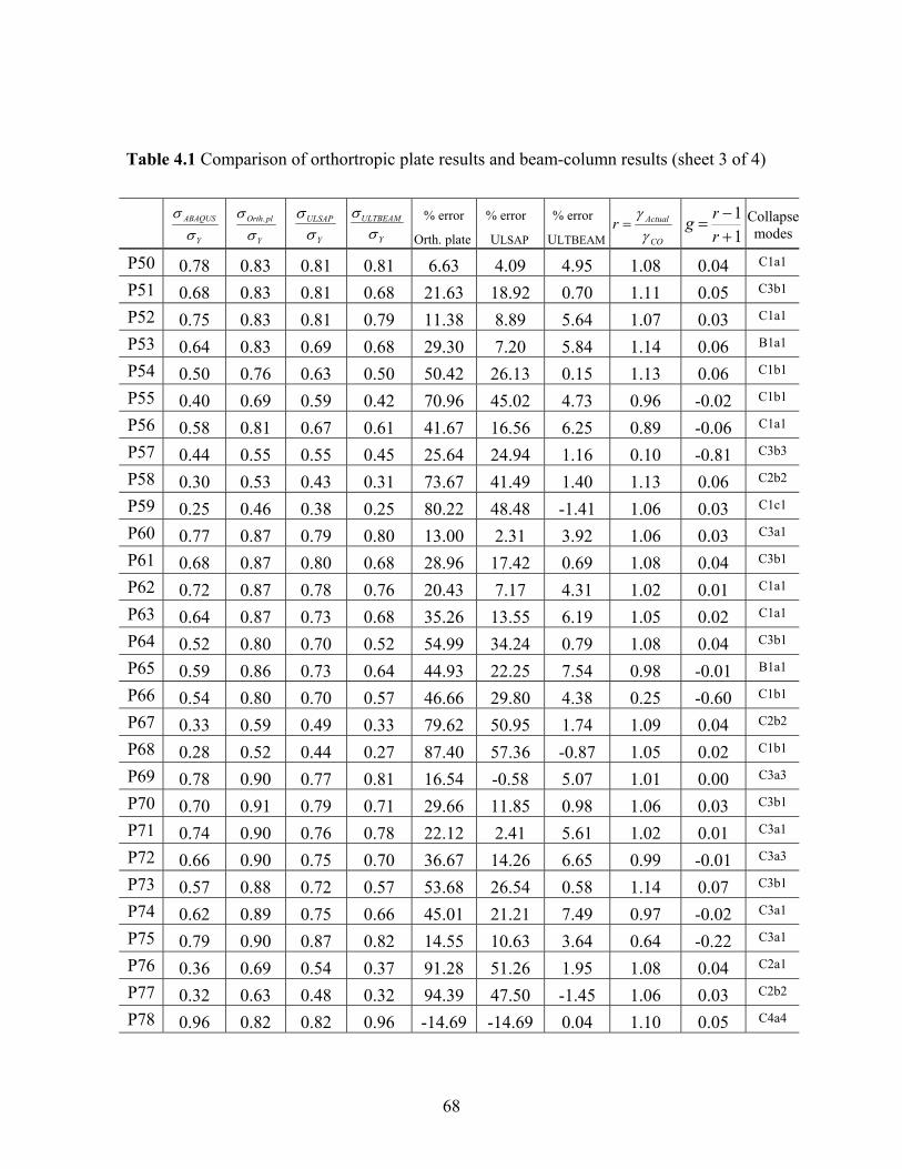
68
Table 4.1 Comparison of orthortropic plate results and beam-column results (sheet 3 of 4)
Y
ABAQUS
σσ
Y
plOrth
σσ .
Y
ULSAP
σσ
Y
ULTBEAM
σσ % error
Orth. plate
% error
ULSAP
% error
ULTBEAM CO
Actualrγ
γ=
11
+−=
rrg Collapse
modes
P50 0.78 0.83 0.81 0.81 6.63 4.09 4.95 1.08 0.04 C1a1
P51 0.68 0.83 0.81 0.68 21.63 18.92 0.70 1.11 0.05 C3b1
P52 0.75 0.83 0.81 0.79 11.38 8.89 5.64 1.07 0.03 C1a1
P53 0.64 0.83 0.69 0.68 29.30 7.20 5.84 1.14 0.06 B1a1
P54 0.50 0.76 0.63 0.50 50.42 26.13 0.15 1.13 0.06 C1b1
P55 0.40 0.69 0.59 0.42 70.96 45.02 4.73 0.96 -0.02 C1b1
P56 0.58 0.81 0.67 0.61 41.67 16.56 6.25 0.89 -0.06 C1a1
P57 0.44 0.55 0.55 0.45 25.64 24.94 1.16 0.10 -0.81 C3b3
P58 0.30 0.53 0.43 0.31 73.67 41.49 1.40 1.13 0.06 C2b2
P59 0.25 0.46 0.38 0.25 80.22 48.48 -1.41 1.06 0.03 C1c1
P60 0.77 0.87 0.79 0.80 13.00 2.31 3.92 1.06 0.03 C3a1
P61 0.68 0.87 0.80 0.68 28.96 17.42 0.69 1.08 0.04 C3b1
P62 0.72 0.87 0.78 0.76 20.43 7.17 4.31 1.02 0.01 C1a1
P63 0.64 0.87 0.73 0.68 35.26 13.55 6.19 1.05 0.02 C1a1
P64 0.52 0.80 0.70 0.52 54.99 34.24 0.79 1.08 0.04 C3b1
P65 0.59 0.86 0.73 0.64 44.93 22.25 7.54 0.98 -0.01 B1a1
P66 0.54 0.80 0.70 0.57 46.66 29.80 4.38 0.25 -0.60 C1b1
P67 0.33 0.59 0.49 0.33 79.62 50.95 1.74 1.09 0.04 C2b2
P68 0.28 0.52 0.44 0.27 87.40 57.36 -0.87 1.05 0.02 C1b1
P69 0.78 0.90 0.77 0.81 16.54 -0.58 5.07 1.01 0.00 C3a3
P70 0.70 0.91 0.79 0.71 29.66 11.85 0.98 1.06 0.03 C3b1
P71 0.74 0.90 0.76 0.78 22.12 2.41 5.61 1.02 0.01 C3a1
P72 0.66 0.90 0.75 0.70 36.67 14.26 6.65 0.99 -0.01 C3a3
P73 0.57 0.88 0.72 0.57 53.68 26.54 0.58 1.14 0.07 C3b1
P74 0.62 0.89 0.75 0.66 45.01 21.21 7.49 0.97 -0.02 C3a1
P75 0.79 0.90 0.87 0.82 14.55 10.63 3.64 0.64 -0.22 C3a1
P76 0.36 0.69 0.54 0.37 91.28 51.26 1.95 1.08 0.04 C2a1
P77 0.32 0.63 0.48 0.32 94.39 47.50 -1.45 1.06 0.03 C2b2
P78 0.96 0.82 0.82 0.96 -14.69 -14.69 0.04 1.10 0.05 C4a4
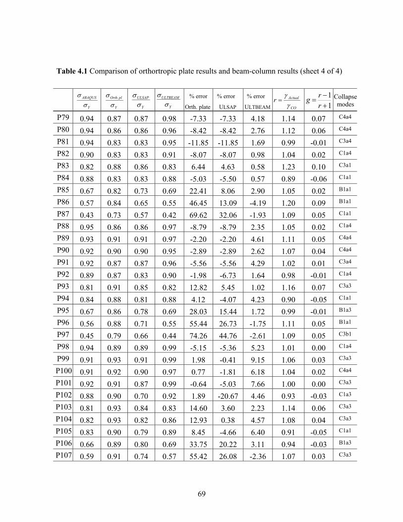
69
Table 4.1 Comparison of orthortropic plate results and beam-column results (sheet 4 of 4)
Y
ABAQUS
σσ
Y
plOrth
σσ .
Y
ULSAP
σσ
Y
ULTBEAM
σσ % error
Orth. plate
% error
ULSAP
% error
ULTBEAM CO
Actualrγ
γ=
11
+−=
rrg Collapse
modes
P79 0.94 0.87 0.87 0.98 -7.33 -7.33 4.18 1.14 0.07 C4a4
P80 0.94 0.86 0.86 0.96 -8.42 -8.42 2.76 1.12 0.06 C4a4
P81 0.94 0.83 0.83 0.95 -11.85 -11.85 1.69 0.99 -0.01 C3a4
P82 0.90 0.83 0.83 0.91 -8.07 -8.07 0.98 1.04 0.02 C1a4
P83 0.82 0.88 0.86 0.83 6.44 4.63 0.58 1.23 0.10 C3a1
P84 0.88 0.83 0.83 0.88 -5.03 -5.50 0.57 0.89 -0.06 C1a1
P85 0.67 0.82 0.73 0.69 22.41 8.06 2.90 1.05 0.02 B1a1
P86 0.57 0.84 0.65 0.55 46.45 13.09 -4.19 1.20 0.09 B1a1
P87 0.43 0.73 0.57 0.42 69.62 32.06 -1.93 1.09 0.05 C1a1
P88 0.95 0.86 0.86 0.97 -8.79 -8.79 2.35 1.05 0.02 C1a4
P89 0.93 0.91 0.91 0.97 -2.20 -2.20 4.61 1.11 0.05 C4a4
P90 0.92 0.90 0.90 0.95 -2.89 -2.89 2.62 1.07 0.04 C4a4
P91 0.92 0.87 0.87 0.96 -5.56 -5.56 4.29 1.02 0.01 C3a4
P92 0.89 0.87 0.83 0.90 -1.98 -6.73 1.64 0.98 -0.01 C1a4
P93 0.81 0.91 0.85 0.82 12.82 5.45 1.02 1.16 0.07 C3a3
P94 0.84 0.88 0.81 0.88 4.12 -4.07 4.23 0.90 -0.05 C1a1
P95 0.67 0.86 0.78 0.69 28.03 15.44 1.72 0.99 -0.01 B1a3
P96 0.56 0.88 0.71 0.55 55.44 26.73 -1.75 1.11 0.05 B1a1
P97 0.45 0.79 0.66 0.44 74.26 44.76 -2.61 1.09 0.05 C3b1
P98 0.94 0.89 0.89 0.99 -5.15 -5.36 5.23 1.01 0.00 C1a4
P99 0.91 0.93 0.91 0.99 1.98 -0.41 9.15 1.06 0.03 C3a3
P100 0.91 0.92 0.90 0.97 0.77 -1.81 6.18 1.04 0.02 C4a4
P101 0.92 0.91 0.87 0.99 -0.64 -5.03 7.66 1.00 0.00 C3a3
P102 0.88 0.90 0.70 0.92 1.89 -20.67 4.46 0.93 -0.03 C1a3
P103 0.81 0.93 0.84 0.83 14.60 3.60 2.23 1.14 0.06 C3a3
P104 0.82 0.93 0.82 0.86 12.93 0.38 4.57 1.08 0.04 C3a3
P105 0.83 0.90 0.79 0.89 8.45 -4.66 6.40 0.91 -0.05 C1a1
P106 0.66 0.89 0.80 0.69 33.75 20.22 3.11 0.94 -0.03 B1a3
P107 0.59 0.91 0.74 0.57 55.42 26.08 -2.36 1.07 0.03 C3a3

70
-40
-20
0
20
40
60
80
100
120
-1.0 -0.8 -0.6 -0.4 -0.2 0.0 0.2 0.4 0.6 0.8 1.0
ULSAP-Pure orth. platemethod
ULSAP-Weighted averageorth. plate method
Beam-column method
Figure 4.1 Percent error of orthotropic plate and beam-column approaches relative to FEA
% error
11
+−
=rrg

71
Table 4.2 statistical comparisons of orthotropic plate results and beam-column results
Mean error COV ULSAP – Pure Orth. Method 33.25 % 0.224
ULSAP – Weighted Average Orth. Method 17.5 % 0.152
Beam-column method 3.32 % 0.039
4.2 Discussion of Results
Table 4.1 shows the accuracy (percent error) of the orthotropic plate, ULSAP and
beam-column results relative to the ABAQUS nonlinear FE results for all 107 panels.
The statistical results are summarized in Table 4.2 and the error values are plotted in
Figure 4.1. At first they were plotted versus the ratio of the actual γ to the crossover
value: COActual γγ . However, this gives a skewed distribution because the panels with
relatively low elastic overall buckling stress (small stiffeners and therefore small γ) are
confined to the range 0 < r < 1, whereas panels with large elastic overall buckling stress
(large stiffeners) extend over the range 1 < r < ¶. In order to eliminate the skew a new
parameter is introduced:” and “ULSAP – Weighted Average Orthotropic Method
11
+−
=rrg (4.1)
For g the variation is normalized: -1 < g < 1, with g = 0 corresponding to crossover
panels. Therefore g is used as the horizontal axis in Figure 4.1.
Table 4.2 and Fig 4.1, which pertain to all 107 panels, reveal some very interesting
results:
(i) They verify that the “pure” orthotropic plate method is very optimistic (mean
error 33.25 %, COV 0.224).

72
(ii) The ULSAP “weighted average” method is better (mean error 17.5 %, COV
0.152).
(iii) The beam-column method is the most accurate (mean error 3.32 %, COV
0.039).
(iv) For panels in the range -0.1 < g < +0.1 (i.e. for crossover panels) the ULSAP
method has large positive errors (optimistic, up to 57%), even after discounting
the effect of the stiffeners by roughly 50%, by averaging with an unstiffened
panel.
(v) The beam-column method maintains its accuracy for all values of g; there is no
deterioration for crossover panels.
Observations (i)-(iv) are discussed in the next section. Observation (v) can be
explained by the fact that the concept and definition of a crossover panel is based on
purely elastic buckling. Therefore crossover proportions (g º1) have no significance for:
(i) typical ship panels, which buckle inelastically; (ii) the beam-column method, which
allows fully for the occurrence and spread of plasticity.
4.2.1 Possible Causes of Error in the Orthotropic-Based Methods
We now consider what might be the reasons for the above error. In using the
orthotropic plate theory for ultimate strength, the crucial hypothesis is that collapse
coincides with the first occurrence of yield at the “outer surface”, which is at a distance
equal to one-half of the equivalent plate thickness from the midthickness. It thereby
makes an allowance for a bending component of stress. However, this distance is much
less than the physical distance from the neutral axis for longitudinal bending to the
stiffener flange, denoted as zflange.
Since both the “pure” and Weighted Average orthotropic methods associate collapse
with initial yield, they do not consider the growth and spreading of plasticity, and this is
the basis for using elastic theory. Orthotropic plate theory is based on a regular buckled

73
pattern of m x n half waves. If the stiffeners are small it will correctly predict overall
buckling, with m and n being small (usually 1). If the stiffeners are large it will correctly
predict local plate buckling, with m being roughly B/(ns+1) where ns is the number of
stiffeners. But in a crossover panel these two buckling modes are occurring together and
orthotropic plate theory does not allow for two simultaneous elastic buckling modes. This
could well be a source of the error. However, plate buckling is only relevant for the
plate-induced failure mode. Orthotropic plate theory cannot distinguish between plate-
induced and stiffener-induced failure. Also, none of the panels in this study underwent
plate-induced failure. Therefore, even if a crossover condition causes an error in the
orthotropic plate approach, there may be other additional causes of error.
Since the orthotropic plate approach deteriorates so markedly for crossover panels, it
is of interest to separate the results into two groups: crossover panels (-0.1 < g < 0.1) and
all others. In all, there are 58 panels within this range of g. Within this group there are
six panels for which the plate slenderness parameter β is 3.73. For ship panels this is
unusually slender and it permits the stiffeners to act independently, which by itself is
sufficient reason for the orthotropic plate approach to have less accuracy. Therefore
these six panels have been removed from the crossover group. Figures 4.2 and 4.3 give
the results for the remaining 52 panels. Since these are all crossover panels, there is no
point in keeping g as the horizontal axis.
In searching for another structure parameter that might influence the accuracy of the
orthotropic plate theory, we recall that at the beginning of Section 4.2.1 we noted that the
initial yield is taken as occurring at the orthotropic “surface”, and this involves a distance
from the midthickness that is much less than the physical distance zflange from the neutral
axis of the stiffener-plate section to the stiffener flange. The maximum bending stress is
proportional to the inverse of the section modulus Z = I / zflange. Therefore, the large
overestimate of ultimate strength could be due to the overestimate of 1/Z. To investigate
this, Figs 4.2 and 4.3 plot the error in the ULSAP weighted average method for the 52
panels versus the ratio b2t/Z. For the 3-stiffener panels (Figure 4.2), there is a definite

74
correlation whereas for the 5-stiffener panels (Figure 4.3) the correlation is less
pronounced.
-10
0
10
20
30
40
50
0 20 40 60 80 100 120 140 160 180 200
Figure 4.2 Percent error of ULSAP for 3-stiffener “crossover” panels against Ztb /2
Ztb2
% error ULSAP with FEA

75
-30
-20
-10
0
10
20
30
40
50
0 10 20 30 40 50 60 70 80 90 100
Figure 4.3 Percent error of ULSAP for 5-stiffener “crossover” panels against Ztb /2
Ztb2
% error ULSAP with FEA

76
4.2.2 Collapse mechanism for “crossover” panels In an attempt to broadly classify the collapse mechanism for the 55 “crossover”
panels from Table 4.1, the panels P50 to P107 (excluding P57, P66 and P75) are grouped
as under:
END BAYS
PLATE
ELASTIC
END BAYS
PLATE
YIELDED
MID BAY
PLATE
ELASTIC
Group I C1a1 (9) C1c1 (1) B1a1 (5) C1b1 (3) ------ 18
Group II C1a3 (1) B1a3 (2) C1a4 (4) ------ 7
MID BAY
PLATE
YIELDED
Group III C2a1 (1) C3a1 (4) C3b1 (6) ------ 11
Group IV C2b2 (3) C3a3 (8) C3a4 (2) C4a4 (6) ------ 19
The ABAQUS Von Mises stress distribution at the maximum load carrying capacity
of one panel from each group is shown in the following figures:

77
Figure 4.4 P52 (Group I), =ultx,σ 263.3 MPa
Figure 4.5 P82 (Group II), =ultx,σ 318.0 MPa
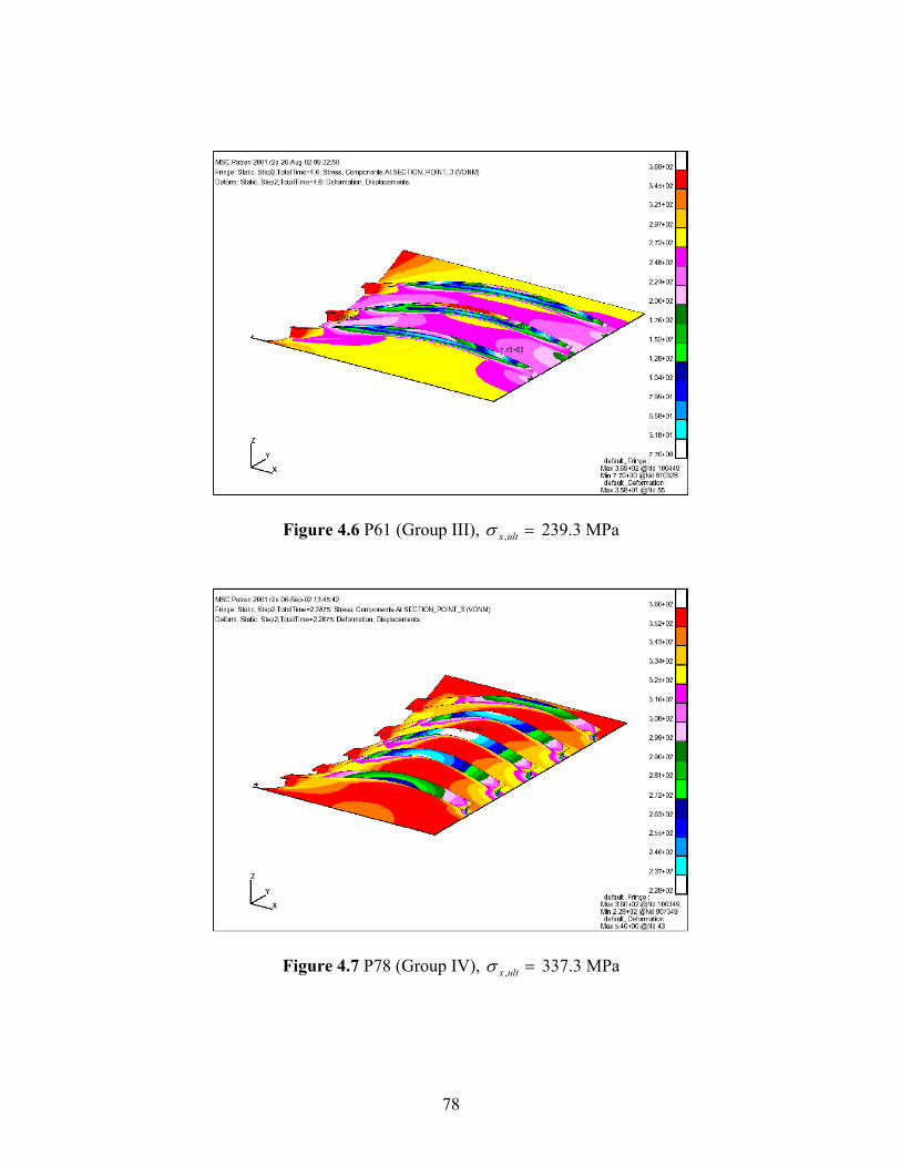
78
Figure 4.6 P61 (Group III), =ultx,σ 239.3 MPa
Figure 4.7 P78 (Group IV), =ultx,σ 337.3 MPa

79
Chapter 5
Ultimate Strength of Stiffened Panels under Transverse Compression
Based on the observations from nonlinear finite element solutions, a new numerical
method for calculating the ultimate strength of stiffened panels under transverse
compression with and without pressure is developed. The method is based on a further
extension of the nonlinear beam-column theory presented in Chapter 2.
5.1 Nonlinear FE Investigations
Using ABAQUS, ultimate strength analyses have been performed on a typical ship
panel called “dw5120”, subjected to transverse axial compression, with and without
pressure, which has also been analyzed by the ship classification society Det Norske
Veritas. Following are the particulars of the finite element model:
Model dimensions
Length of each bay: 5120 mm
No. of bays modeled: ½ + 1 + 1 + ½
Stiffeners: 9 longitudinal T-stiffeners
Panel breadth: 9100 mm Plate thickness: 20 mm
Web height: 598.5 mm Web thickness: 12 mm
80
Flange breadth: 200 mm Flange thickness: 20 mm
Material properties
Material of plate and stiffeners: Steel
Yield stress: 315 MPa
Young’s modulus: 208000 N/mm2
Poisson’s ratio: 0.3
Finite elements
Type of elements: S4
No. of elements in plate: 102 x 6 per stiffener
No. of elements in web: 102 x 5 per stiffener
No. of elements in flange: 102 x 2 per stiffener
Boundary conditions
Let a “0” on T [x,y,z] denote translation constraints and R [x,y,z] denote rotational
constraints about x, y and z coordinates.
• The short edges have symmetric boundary conditions being simulated with
R [ ,0,0] and all nodes having the same x-displacement. The latter is achieved
using the *EQUATION option.
• The panel is clamped along the long edges, being simulated with R [0,0,0] and
all nodes having the same y-displacement. The latter is achieved using the
*EQUATION option.
• The middle frame is not modeled but symmetric boundary conditions are
simulated with T [0, ,0] and R [ ,0, ].
• The other two transverse frames are also not modeled but simulated with T [ ,
,0].

81
• As the stiffeners pass through the three frames, they are constrained to remain
vertical by using the *EQUATION option for equal y-displacement at all
stiffener nodes at the frame locations.
Loads
The uniaxial transverse compressions are applied as concentrated nodal forces using
the *CLOAD option.
The lateral pressure is applied as a distributed pressure on the plate side using the
*DLOAD option.
The pressure and initial portion of the in-plane axial loads are applied first, as a
“dead load”, and then the in-plane loads are incremented by a common factor.
Imperfections
The imperfections to the “perfect” model are applied using the *IMPERFECTION,
INPUT = filename option. The imperfection file contains the node numbers with their x,
y and z imperfection values. These imperfection values are the sum of the following:
• Local imperfection, which is the initial imperfection of each subpanel (plating
between the stiffeners). This local imperfection is obtained from an eigenvalue
buckling mode shape using the *BUCKLE option as shown in Figure 5.1. The
applied load is equal biaxial in-plane compression. The mode shape is shown in
Figure 5.1. This mode shape is scaled to have a maximum vertical deflection in
the plate equal to 0.1b2t (6.27 mm, which is an average value according to Smith,
1988).
• Global imperfection in the stiffeners, generated with an alternating sine-
deflection equation, with a maximum deflection in the z-direction equal to
1/1000 of the stiffener span (5.12 mm). The global imperfection is applied in an
alternating up-down pattern so that the stiffener deflection is negative at
x = - L/2 and positive at x = + L/2, where x is measured from a frame location
and L is the length of one bay (5120 mm).

82
Figure 5.1 Eigenvalue Buckling Analysis, Mode 1 Eigenvalue = 110.12
Results and observations
Two load cases are studied: Case 1 is panel under compression yσ only, without
pressure. Case 2 is panel under combined compression and lateral pressure (p = 0.2531
MPa).
For case 1, ultimate strength is 120 MPa (Figure 5.2, 5.3). Collapse is due to
buckling of all subpanels, in alternating directions, with full yield along their short edges.
The initial tilt of the stiffeners is magnified but there is no yielding in the flange, and the
stiffeners are not involved in the collapse. Their only role is to provide w = 0 restraint to
the plating.
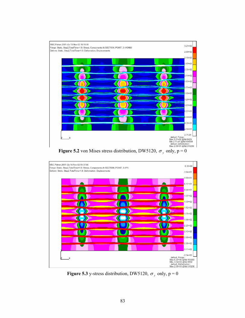
83
Figure 5.2 von Mises stress distribution, DW5120, yσ only, p = 0
Figure 5.3 y-stress distribution, DW5120, yσ only, p = 0
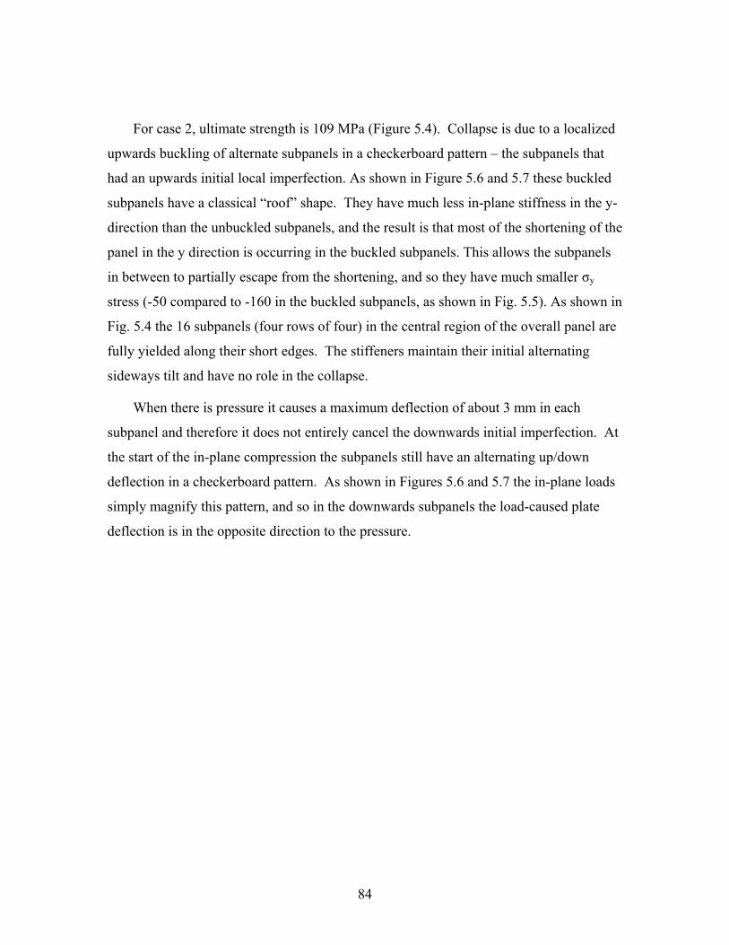
84
For case 2, ultimate strength is 109 MPa (Figure 5.4). Collapse is due to a localized
upwards buckling of alternate subpanels in a checkerboard pattern – the subpanels that
had an upwards initial local imperfection. As shown in Figure 5.6 and 5.7 these buckled
subpanels have a classical “roof” shape. They have much less in-plane stiffness in the y-
direction than the unbuckled subpanels, and the result is that most of the shortening of the
panel in the y direction is occurring in the buckled subpanels. This allows the subpanels
in between to partially escape from the shortening, and so they have much smaller σy
stress (-50 compared to -160 in the buckled subpanels, as shown in Fig. 5.5). As shown in
Fig. 5.4 the 16 subpanels (four rows of four) in the central region of the overall panel are
fully yielded along their short edges. The stiffeners maintain their initial alternating
sideways tilt and have no role in the collapse.
When there is pressure it causes a maximum deflection of about 3 mm in each
subpanel and therefore it does not entirely cancel the downwards initial imperfection. At
the start of the in-plane compression the subpanels still have an alternating up/down
deflection in a checkerboard pattern. As shown in Figures 5.6 and 5.7 the in-plane loads
simply magnify this pattern, and so in the downwards subpanels the load-caused plate
deflection is in the opposite direction to the pressure.
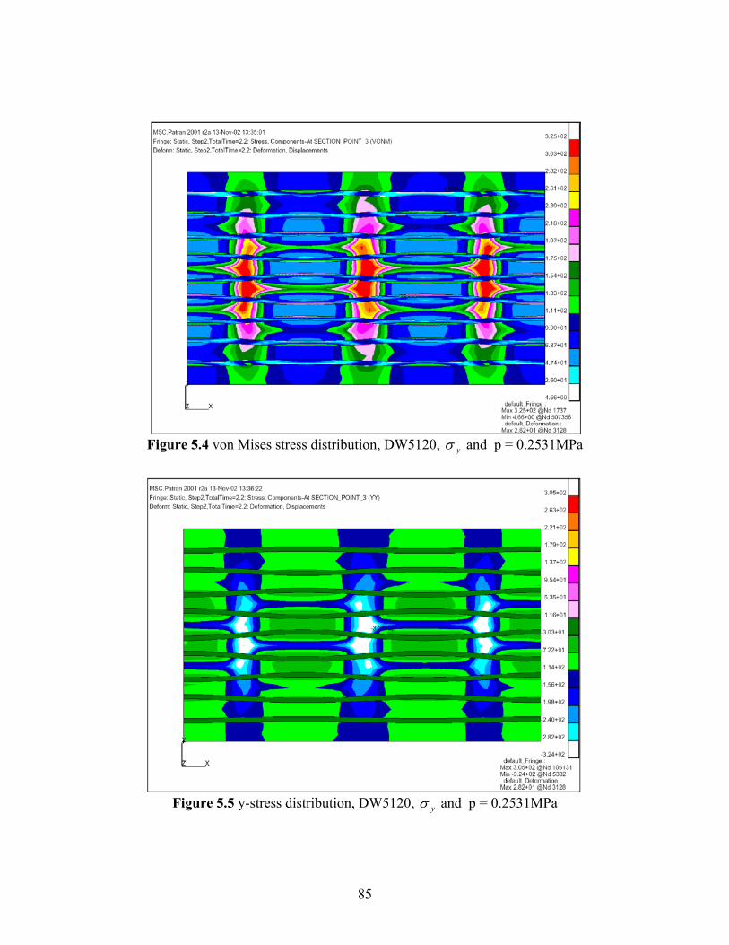
85
Figure 5.4 von Mises stress distribution, DW5120, yσ and p = 0.2531MPa
Figure 5.5 y-stress distribution, DW5120, yσ and p = 0.2531MPa

86
Figure 5.6 vertical (z) displacement, DW5120, yσ and p = 0.2531MPa
Figure 5.7 side view of displacements, DW5120, yσ and p = 0.2531MPa
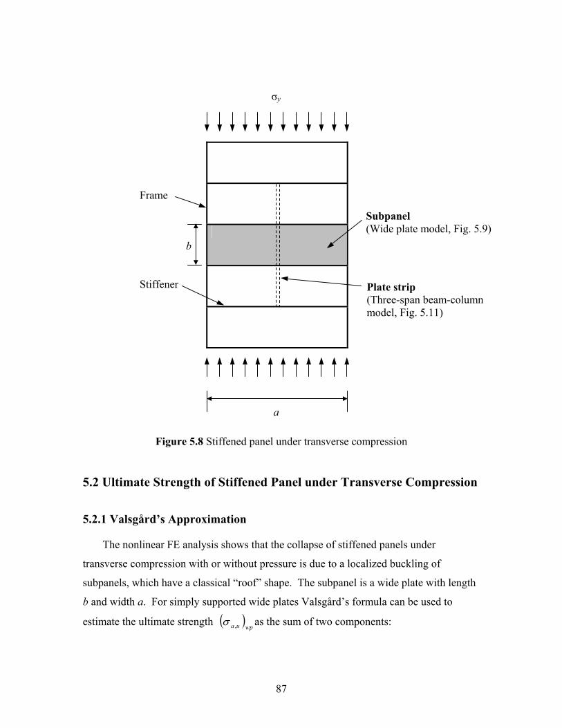
87
Figure 5.8 Stiffened panel under transverse compression
5.2 Ultimate Strength of Stiffened Panel under Transverse Compression
5.2.1 Valsgård’s Approximation
The nonlinear FE analysis shows that the collapse of stiffened panels under
transverse compression with or without pressure is due to a localized buckling of
subpanels, which have a classical “roof” shape. The subpanel is a wide plate with length
b and width a. For simply supported wide plates Valsgård’s formula can be used to
estimate the ultimate strength ( )wpua,σ as the sum of two components:
Frame Stiffener
Subpanel (Wide plate model, Fig. 5.9)
Plate strip (Three-span beam-column model, Fig. 5.11)
σy
b
a

88
( ) ( ) ( )wcuaLuawpua a
bab
,,, 1 σσσ
−+= (5.1)
where ( )Lua,σ is the ultimate strength of the two end portions each of width b/2 which
together make up a square plate (b x b) and ( )wcua,σ is the ultimate strength of the center
part of the plate, which is effectively a “wide column”.
Figure 5.9 Valsgård’s approximation (Hughes, 1988)
Valsgård’s original method was for wide plates that are simply supported on all four
edges. For stiffened panels subjected to a lateral pressure the edge condition is in
between simply supported and clamped. To apply the Valsgård approximation to a
stiffened panel under transverse compression, we need to find new formulas for ( )Lua,σ
and ( )wcua,σ , which can match the real boundary conditions of a subpanel.
From nonlinear FE solutions, curves for ultimate strength of a clamped square plate
are developed in Section 5.2.2, which is applicable to get ( )Lua,σ for subpanels.
b
a
b
b/2
b/2
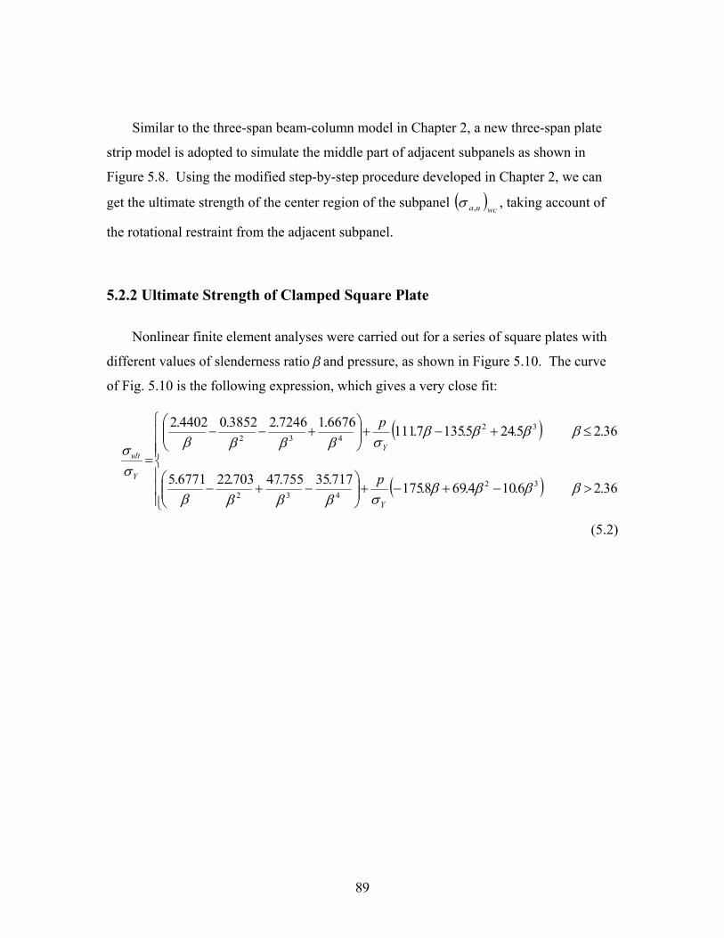
89
Similar to the three-span beam-column model in Chapter 2, a new three-span plate
strip model is adopted to simulate the middle part of adjacent subpanels as shown in
Figure 5.8. Using the modified step-by-step procedure developed in Chapter 2, we can
get the ultimate strength of the center region of the subpanel ( )wcua,σ , taking account of
the rotational restraint from the adjacent subpanel.
5.2.2 Ultimate Strength of Clamped Square Plate
Nonlinear finite element analyses were carried out for a series of square plates with
different values of slenderness ratio b and pressure, as shown in Figure 5.10. The curve
of Fig. 5.10 is the following expression, which gives a very close fit:
( )
( )
>−+−+
−+−
≤+−+
+−−
=
36.26.104.698.175717.35755.47703.226771.5
36.25.245.1357.1116676.17246.23852.04402.2
32432
32432
ββββσββββ
ββββσββββ
σσ
Y
Y
Y
ult
p
p
(5.2)
90
Figure 5.10 Clamped square plates under compression and pressure
5.2.3 Ultimate Strength of Continuous Plate Strip
Consider a plate strip in the middle of three adjacent subpanels as shown in Figure
5.11. The only difference between the plate strip model and the continuous beam-column
model in Figure 2.8 is the boundary conditions at the ends, which are clamped-clamped
here and pinned-pinned in Fig. 2.8.

91
Figure 5.11 The plate strip model
s
dp
s
b b b
Clamped Clamped
MR
s Mmid
w1 + dp
p
s
Stress distribution at the cross section at Midlength
-sY 0
-sY 0
Stress distribution at the cross section at the end
t
Symbols indicate the integration points in ABAQUS
Midlength The end of the middle strip

92
The subpanel in which the initial deflection is in the same direction as the applied
pressure is the weakest one. In Fig. 5.11 the pressure is applied downward on the plate
strip model and therefore the middle plate strip is of main interest.
As shown in Fig. 5.11, there will be a reaction moment MR at the end of the middle
plate strip. The magnitude of the reaction moment MR indicates how much rotational
restraint is provided by the adjacent plate strip. Previous models of subpanels have
assumed simple support, i.e. MR = 0, which results in a pessimistic prediction of ultimate
strength. This continuous three-span plate strip model is developed to allow for the
rotational restraint.
No pressure
Collapse will occur at the midlength of the middle plate strip. The end plate strips
will remain elastic. Using the principle of superposition, we can get the slope qend (refer
to Figure 2.8) of the plate strip:
aka
ka
kak
aka
kaEIk
M pRend
πφδθ +
−
−
−−=
tan1
sin1
tan1
2
2 (5.3)
Applying the numerical procedure developed in Section 2.4.3 with this new
expression for qend, we obtain the reaction moment MR0 and the ultimate strength of the
plate strip sult_p0, which can be used in place of ( )wcua ,σ in eq. (5.1).
With pressure
With pressure, yielding may occur at the end of the middle strip, and the end strip
will not remain elastic at collapse. Hence, the forgoing procedure is no longer applicable.
However, the simplicity of the rectangular cross section shape of a plate strip makes it
possible to study the inelastic behavior at collapse in detail, so that reasonable
approximations can be made to get the solution.

93
For a plate strip under ultimate load sult, the following three moments can be
accurately evaluated:
1. Initial yielding moment, MIY. (sU = sY in Fig. 2.2(a))
( )6
2tM ultYIY σσ −= (5.4)
2. Initial secondary plastic moment, MISP. (sU = sY, sL = -sY in Fig. 2.2(b)
( )
+−=
Y
ultultYISP
tMσσ
σσ2
16
2
(5.5)
3. Perfect plastic hinge moment, MPH, defined in Eq. 2.12. (Fig. 2.2(d))
Nonlinear FE analyses were carried out for the plate strip in panel DW5120 with
transverse compression and different pressure. Half of the plate strip in Fig. 5.11 was
modeled, and beam elements (B21) were used. From ABAQUS, we can read the stresses
at integration points as shown in Fig. 5.11. Fig. 5.12 shows the stress distribution
patterns for this plate strip under compression and various pressures (p = 0.0, 0.05, 0.10,
0.15, 0.20, 0.25, 0.30 MPa).

94
Figure 5.12 Stress distributions under different pressure
It can be seen in Fig. 5.12(a) that the applied pressure has very little influence on the
stress distribution at the midlength, which remains close to the initial secondary plastic
situation. Based on this observation, we assume that Mmid º MISP at collapse.
On the other hand, at the end of the middle strip, the stress distribution is changing as
the pressure varies: when there is no pressure, the whole cross section remains elastic; as
pressure increases, the cross section first becomes primary plastic, and then secondary
plastic. This means that as pressure increases, the reaction moment MR at collapse will
increase. The lower limit of MR is MR0 ( ≤ MIY ), which corresponds to the zero pressure
case. The upper limit should be MPH, which is the perfect plastic hinge moment.
According to eq. (16.2.8) in (Hughes, 1988), the pressure on the plate strip at the
completion of the perfect plastic hinge is:
0
t
sY -sY
0
p=0.20 MPa
p=0.25 MPa
p=0.30 MPa
p=0.0 MPa
p=0.05 MPa
p=0.10 MPa
p=0.15 MPa
Seven lines corresponding to seven pressure cases.
(a) At midlength (b) At the end of the middle strip

95
2
12bMp PH
PH = (5.6)
Notice that the unit width is omitted in the denominator, and the units of the right hand
side of eq. (5.6) are [Force/Length2]. A parabolic variation of MR with pressure p is then
assumed:
( )02
2
)()(
RPHPH
PHPHR MM
pppMM −
−−= (5.7)
which is the curve shown in Fig. 5.13
Figure 5.13 Parabolic variation of MR with pressure (p)
From the moment equilibrium condition at the midlength of the middle plate strip,
get the maximum displacement w1 at collapse:
pult
Rmid
t
pbMMw δ
σ−
−+= 8
2
1 (5.8)
Then we have enough information to start the numerical integration method to
determine sult. Figure 5.14 illustrates the whole procedure for solving ultimate strength
sult of the plate strip under compression and pressure.
p
MR
MPH
MR0
0 0 pPH

96
Figure 5.14 Numerical procedure for plate strip
wn = 0 ?
Guess initial sult
Mmid = MISP
Get MR from Eq. 5.7
Step-by-step procedure s M f wi+1 wn
No
YesAdjust sult
Get w1 from Eq. 5.8
Set p = 0 Do procedure in Fig. 2.10 with Eq. 5.3 for qendGet sult_p0 and MR0
Actural p = 0 ? Yes
No
sult = sult_p0

97
5.3 Verification
Ultimate strength analyses of panel DW5120 under transverse compression with
various values of pressure were carried out using the plate strip approach. Six other
three-bay panels with different plate thickness and different stiffener sizes selected from
Table 1.1 were also analyzed.
The results are compared with the ABAQUS solutions in Table 5.1. The mean
absolute percentage error is 3.3% and COV = 0.044.

98
Table 5.1 Comparison of plate strip approach with the FEA solutions for transverse compression capacity of stiffened panels
P (MPa) Y
ULTBEAM
σσ
Y
ABAQUS
σσ % error
ULTBEAM ABAQUS
ULTBEAM
σσ
0 0.381 0.381 0.037 1.000 0.05 0.378 0.365 3.668 1.037 0.10 0.376 0.365 2.968 1.030 0.15 0.373 0.343 8.890 1.089 0.20 0.361 0.356 1.547 1.015 0.25 0.338 0.346 -2.375 0.976
DW5120
0.30 0.311 0.333 -6.644 0.934 0 0.489 0.473 3.460 1.035
0.123 0.478 0.466 2.701 1.027 0.245 0.462 0.451 2.415 1.024
P8
0.368 0.417 0.431 -3.261 0.967 0 0.378 0.368 2.614 1.026
0.079 0.365 0.366 -0.264 0.997
P14
0.157 0.352 0.357 -1.157 0.988 0 0.237 0.242 -1.990 0.980
0.031 0.231 0.241 -4.095 0.959
P20
0.061 0.225 0.244 -7.816 0.922 0 0.621 0.601 3.404 1.034
0.304 0.574 0.584 -1.708 0.983
P32
0.456 0.552 0.550 0.392 1.004 0 0.483 0.482 0.093 1.001
0.176 0.476 0.458 3.890 1.039
P38
0.264 0.456 0.406 12.524 1.125 0 0.281 0.287 -2.264 0.977
0.069 0.273 0.281 -3.184 0.968
P44
0.103 0.268 0.274 -2.053 0.979

99
Chapter 6
Concluding Remarks
In the current research, we have shown how the inelastic beam-column theory can be
applied to predict the ultimate strength of stiffened panels with two load cases: under
longitudinal compression and under transverse compression.
An improved step-by-step integration method for beam-columns was presented in
Chapter 2. This numerical method can analyze the inelastic beam-column under axial
compression, uniform lateral load, end moments, and combined loads. A special
procedure for three-span beam-columns was also developed with a special attention to
usability for stiffened panels. A Fortran program, ULTBEAM, was developed as an
implementation of this method. The comparison of ULTBEAM with a nonlinear finite
element analysis (ABAQUS) showed very good agreement. Currently, only beam-
columns with rectangular and monosymmetric I cross sections can be analyzed. The
method can be extended to other types of cross section, by deriving similar M- F -P
relationships.
The improved beam-column method was first applied for the ultimate strength
analysis of a stiffened panel under longitudinal compression. Based on nonlinear finite
element results, a correction factor was found to apply ULTBEAM to stiffened panels.
The elasto-plastic finite element ultimate strength analyses were performed for 107 three-
bay stiffened panels, covering a wide range of panel length, plate thickness, and stiffener
sizes and proportions. It has been shown that the three-bay simply supported model is

100
sufficiently general to apply to any panel with three or more bays. An empirical formula
for effective breadth was found to allow for local plate buckling. The numerical
procedure for ultimate strength analysis of a stiffened panel under longitudinal
compression could be summarized as follows:
1. Calculate effective breadth of the local plating, be;
2. Apply ULTBEAM, get ultimate strength of the isolated stiffener-plate
combination;
3. Apply the correction factor, get ultimate strength of the full panel.
It was shown that this beam-column approach predicts very accurate results for all
107 panels.
Another widely-used approach for ultimate strength analysis of a stiffened panel is
the orthotropic plate method. It was found that this method has poor performance for
“crossover” panels.
The beam-column method can also be applied for the ultimate strength analysis of
stiffened panel under transverse compression, with or without pressure. The fine mesh
finite element investigations with a typical ship panel from DNV revealed that the
collapse of stiffened panels under transverse compression is due to a localized buckling
of subpanels, which have a classical “roof” shape. ULTBEAM can be used to calculate
the ultimate strength of the plate strip representing the center portion of the subpanel.
Curve fitting was performed to predict the ultimate strength of a clamped square plate,
which represents the two side portions of the subpanel. These two ultimate strength
predictions are integrated based on the Valsgård’s approximation to get the ultimate
strength of a stiffened panel under transverse compression. This method was evaluated
by comparing the results with those obtained using ABAQUS, for several typical ship
panels under various pressures.

101
References
ABS (2000). Rules for building and classing steel vessels, American Bureau of
Shipping, Part 5, Houston.
API (2000). Bulletin on design of flat plate structures, API Bulletin 2V, 2nd edition.
Bleich, F. (1952). Buckling strength of metal structures, McGraw-Hill, New York.
Canadian Standards Association. (1994) Limit states design of steel structures,
CAN/CSA S16.1-94, Rexdale, Ontario.
Carlsen, C.A. (1977). Simplified collapse analysis of stiffened plates, Norwegian
Maritime Research, No.4, pp.20-36.
Carlsen, C.A. (1981). A parametric study of collapse of stiffened plates in
compression, The Structural Engineer, Vol.58B, No.2, pp.33-40.
Chatterjee, S. and Dowling, P.J. (1975). Proposed design rules for longitudinal
stiffeners in compression flanges of box girders, Engineering Structure Laboratories,
Civil Engineering Department, Imperial Collage, CESLIC Report BG 40, London, May.
Chen, W.F. and Atsuta, T. (1976, 1977). Theory of beam-columns, Vol.1 and 2,
McGraw-Hill, New York.
Chen, W.F. and Liu, E.M. (1987). Structural stability, theory and implementation,
Elsevier, New York.
Das, P.K. and Garside, J.F. (1991). Structural redundancy for continuous and
discrete systems, Ship Structure Committee, SSC-354.
DNV (1995). Buckling strength analysis, Classification Notes No. 30.1, Det norske
Veritas, Oslo, July.

102
Ellinas, C.P., Supple and Walker, A.C. (1984). Buckling of offshore structures, a
state-of-the-art review, Gulf Publishing Co., Houston.
Faulkner, D. (1975). A review of effective plating for use in the analysis of stiffened
plating in bending and compression, J. of Ship Research, Vol.19, No.1, pp.1-17.
Fujikubo, M. and Yao, T. (1999). Elastic local buckling strength of stiffened plate
considering plate/stiffener interaction and welding residual stress, Marine Structures,
Vol.12, pp.543-64.
Hu, S.Z., Chen, Q., Pegg, N. and Zimmerman, T.J.E. (1997). Ultimate collapse tests
of stiffened plate ship structural units, Marine Structures, Vol.10, pp.587-610.
Hughes, O.F. (1988). Ship structural design, a rationally-based, computer-aided
optimization approach, SNAME, New Jersey.
Hughes, O.F., Nikolaidis, E., Ayyub, B., White, G. and Hess, P. (1994). Uncertainty
in strength models for marine structures, Ship Structure Committee, SSC-375.
Hughes, O.F., Ghosh, B. (2003). Improved prediction of simultaneous local and
overall buckling of stiffened panels (in preparation)
ISSC (2000). Ultimate strength, Proc. of the 14th International Ship and Offshore
Structures Congress, Technical Committee III.1, Vol.1:253-321.
Johansson, B., Maquio, R., Sedlacek, G.. (2001). New design rules for plated
structures in Eurocode 3, J. of Constructional Steel Research, Vol.57, pp.279-311.
Klitchieff, J.M. (1951). On the stability of plates reinforced by longitudinal ribs, J.
Applied Mechanics, 18(4), pp. 221-268.
Paik, J.K. and Kim, D.H. (1997). A benchmark study of the ultimate compressive
strength formulations for stiffened panels, J. of Research Institute of Industrial
Technology, Vol.53, Pusan National University, Busan, pp.373-405.
Paik, J.K., Thayamballi, A.K., Wang, G. and Kim, B.J. (2000). On advanced
buckling and ultimate strength design of ship plating, Trans. SNAME, Vol.108.
Paik, J.K., Thayamballi, A.K. and Kim, B.J. (2001). Large deflection orthotropic
plate approach to develop ultimate strength formulations for stiffened panels under

103
combined biaxial compression / tension and lateral pressure, Thin-Walled Structures,
Vol.39, No.3, pp.215-246
Paik, J.K., Thayamballi, A.K. (2002). Ultimate Limit State Design of Steel Plated
Structures, John Wiley & Sons.
Pradillon, J.Y., Quesnel, T., Toderan, C., and Rigo, P. (2001). Ultimate strength of
longitudinally stiffened panels: multi-criteria comparative analysis, Practical Design of
Ships and Other Floating Structures, 2001, Elsevier, pp.1029-1035.
Rigo, P., Moan, T., Frieze, P.A. and Chryssanthopoulos, M. (1995). Benchmarking
of ultimate strength prediction for longitudinally stiffened panels, Proc. of the 6th
International Symposium on Practical Design of Ship and Mobile Units (PRADS’95),
Vol.2, Seoul, September, pp. 869-882.
Sheikh, I.A., Grondin, G.Y., and Elwi, A.E. (2002). Stiffened steel plates under
uniaxial compression, J. of Constructional Steel Research, Vol.58, pp.1061-1080.
Smith, C.S. (1976). Compressive strength of welded steel ship grillages, Trans.
RINA, Vol.118, pp.325-359.
Smith, C.S., Davidson, P.C., Chapman, J.C., and Dowling, P.J. (1988). Strength and
stiffness of ship’s plating under in-plane compression and tension, Trans. RINA,
Vol.130:277-296.
Smith, C.S., Anderson, N., Chapman, J.C., Davidson, P.C. and Dowling, P.J. (1992).
Strength of stiffened plating under combined compression and lateral pressure, Trans.
RINA, Vol.134, pp.131-147.
Steen, E., Ostvold, T.K., Chapman, J.C., Valsgård, S. (2001). A new design model
for ultimate and buckling strength assessment of stiffened panels, Practical Design of
Ships and Other Floating Structures, 2001, Elsevier, pp.1021-1027.
Timoshenko, S.P., Gere, J.M. (1961). Theory of elastic stability, 2nd edition,
McGraw Hill, New York

104
Tvergaard, V., Needleman, A. (1975). Buckling of eccentrically stiffened elastic-
plastic panels on two simple supports or multiple supported, International Journal Solids
Structures, 11, pp 647.
Valsgård, S. (1979). Ultimate capacity of plates in transverse compression, Det
norske Veritas, Report no. 79-0104

105
Appendix
ABAQUS Stress Distributions
This Appendix contains the color-coded stress distribution gradients in the mid-
thickness of the cross-section of the test panels P1 to P49 at collapse. All the panels were
subjected to uniaxial compression and the commercial finite element program ABAQUS
was used to obtain the ultimate strength, as detailed in Chapter 3. The stress distributions
are obtained from the ABAQUS results read in PATRAN. For every panel, the von Mises
stress and the xσ stress are shown.

106
von Mises stress distribution
x-stress distribution
Figure A P1, =ultx,σ 147.4 MPa

107
von Mises stress distribution
x-stress distribution
Figure A P2, =ultx,σ 149.3 MPa

108
von Mises stress distribution
x-stress distribution
Figure A P3, =ultx,σ 183.2 MPa

109
von Mises stress distribution
x-stress distribution
Figure A P4, =ultx,σ 232.6 MPa
110
von Mises stress distribution
x-stress distribution
Figure A P5, =ultx,σ 183.5 MPa

111
von Mises stress distribution
x-stress distribution
Figure A P6, =ultx,σ 231.2 MPa

112
von Mises stress distribution
x-stress distribution
Figure A P7, =ultx,σ 334.6 MPa

113
von Mises stress distribution
x-stress distribution
Figure A P8, =ultx,σ 277.2 MPa

114
von Mises stress distribution
x-stress distribution
Figure A P9, =ultx,σ 279.1 MPa

115
von Mises stress distribution
x-stress distribution
Figure A P10, =ultx,σ 131.4 MPa

116
von Mises stress distribution
x-stress distribution
Figure A P11, =ultx,σ 136.0 MPa

117
von Mises stress distribution
x-stress distribution
Figure A P12, =ultx,σ 158.4 MPa

118
von Mises stress distribution
x-stress distribution
Figure A P13, =ultx,σ 175.3 MPa

119
von Mises stress distribution
x-stress distribution
Figure A P14, =ultx,σ 165.5 MPa
120
von Mises stress distribution
x-stress distribution
Figure A P15, =ultx,σ 179.0 MPa

121
von Mises stress distribution
x-stress distribution
Figure A P16, =ultx,σ 274.7 MPa

122
von Mises stress distribution
x-stress distribution
Figure A P17, =ultx,σ 268.9 MPa

123
von Mises stress distribution
x-stress distribution
Figure A P18, =ultx,σ 248.1 MPa
124
von Mises stress distribution
x-stress distribution
Figure A P19, =ultx,σ 98.7 MPa

125
von Mises stress distribution
x-stress distribution
Figure A P20, =ultx,σ 105.5 MPa

126
von Mises stress distribution
x-stress distribution
Figure A P21, =ultx,σ 117.4 MPa

127
von Mises stress distribution
x-stress distribution
Figure A P22, =ultx,σ 181.9 MPa

128
von Mises stress distribution
x-stress distribution
Figure A P23, =ultx,σ 167.7 MPa
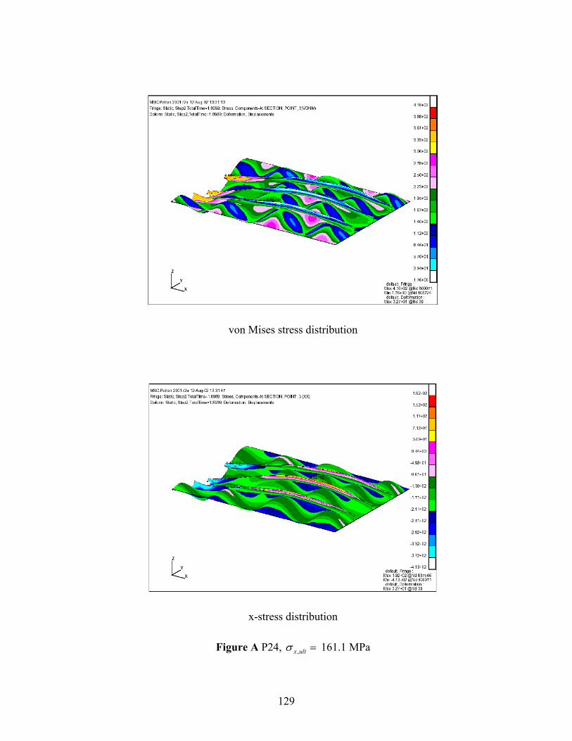
129
von Mises stress distribution
x-stress distribution
Figure A P24, =ultx,σ 161.1 MPa

130
von Mises stress distribution
x-stress distribution
Figure A P25, =ultx,σ 140.6 MPa

131
von Mises stress distribution
x-stress distribution
Figure A P26, =ultx,σ 179.6 MPa

132
von Mises stress distribution
x-stress distribution
Figure A P27, =ultx,σ 159.9 MPa

133
von Mises stress distribution
x-stress distribution
Figure A P28, =ultx,σ 193.7 MPa

134
von Mises stress distribution
x-stress distribution
Figure A P29, =ultx,σ 279.2 MPa

135
von Mises stress distribution
x-stress distribution
Figure A P30, =ultx,σ 225.3 MPa

136
von Mises stress distribution
x-stress distribution
Figure A P31, =ultx,σ 225.3 MPa

137
von Mises stress distribution
x-stress distribution
Figure A P32, =ultx,σ 342.2 MPa

138
von Mises stress distribution
x-stress distribution
Figure A P33, =ultx,σ 313.6 MPa

139
von Mises stress distribution
x-stress distribution
Figure A P34, =ultx,σ 309.8 MPa

140
von Mises stress distribution
x-stress distribution
Figure A P35, =ultx,σ 165.2 MPa

141
von Mises stress distribution
x-stress distribution
Figure A P36, =ultx,σ 149.5 MPa

142
von Mises stress distribution
x-stress distribution
Figure A P37, =ultx,σ 184.1 MPa

143
von Mises stress distribution
x-stress distribution
Figure A P38, =ultx,σ 222.3 MPa

144
von Mises stress distribution
x-stress distribution
Figure A P39, =ultx,σ 204.4 MPa

145
von Mises stress distribution
x-stress distribution
Figure A P40, =ultx,σ 209.1 MPa

146
von Mises stress distribution
x-stress distribution
Figure A P41, =ultx,σ 330.8 MPa

147
von Mises stress distribution
x-stress distribution
Figure A P42, =ultx,σ 321.0 MPa

148
von Mises stress distribution
x-stress distribution
Figure A P43, =ultx,σ 295.3 MPa

149
von Mises stress distribution
x-stress distribution
Figure A P44, =ultx,σ 129.6 MPa

150
von Mises stress distribution
x-stress distribution
Figure A P45, =ultx,σ 140.3 MPa

151
von Mises stress distribution
x-stress distribution
Figure A P46, =ultx,σ 158.0 MPa

152
von Mises stress distribution
x-stress distribution
Figure A P47, =ultx,σ 247.3 MPa

153
von Mises stress distribution
x-stress distribution
Figure A P48, =ultx,σ 234.5 MPa

154
von Mises stress distribution
x-stress distribution
Figure A P49, =ultx,σ 229.5 MPa

155
Vita
Yong Chen was born on September 18, 1974 in Zhijiang County, Hubei Province,
China. He graduated from the No. 1 Middle School of Zhijiang County in July 1992. In
the same year, he began his undergraduate study in Department Naval Architecture and
Ocean Engineering of Huazhong University of Science and Technology (HUST), Wuhan,
China. In July 1996, he graduated with a Bachelor’s degree in engineering and continued
to study in the same institute. He got his Master’s degree in Naval Architecture and
Ocean Engineering in July 1999. Yong Chen came to Virginia Tech in the fall of 1999 to
begin his study toward a PhD with the Department of Aerospace and Ocean Engineering.
This dissertation completes his PhD degree in Aerospace Engineering from Virginia
Tech.