U A

P I T

L B

Thesis submitted inPartial Fulfilment of the

Requirement of the Degree of

Doctor of Philosophy (Ph.D)in Computer Science

by

Ramprasad Saptharishi

Chennai Mathematical InstitutePlot H1 SIPCOT IT ParkPadur PO, Siruseri 603 103

April 2013

Declaration

I declare that the thesis “Unified Approaches to Polynomial Identity Testing and LowerBounds” submitted by me for the degree of Doctor of Philosophy is the record ofwork carried out by me during the period from August 2007 to April 2013 under theguidance of Prof. Manindra Agrawal. is work has not formed the basis for the awardof any degree, diploma, associateship, fellowship, titles in this or any other universityor other similar institution of higher learning.

April 2013 Ramprasad Saptharishi

Chennai Mathematical InstitutePlot H1, SIPCOT IT Park, Siruseri,Kelambakkam 603103India

Certificate

is is to certify that the Ph.D. thesis submitted by Ramprasad Saptharishi to Chen-nai Mathematical Institute, titled “Unified Approaches to Polynomial Identity Testingand Lower Bounds” is a record of bona fide research work done during the period 2007– 2013 under my guidance and supervision. e research work presented in this thesishas not formed the basis for the award of any degree, diploma, associateship, fellow-ship, titles in this institute or any other university or institution of higher learning.

It is further certified that the thesis represents independent work by the candidateand collaboration when existed was necessitated by the nature and scope of problemsdealt with.

Manindra Agrawal(esis superviser)

Chennai Mathematical Institute Indian Institute of TechnologyPlot H1, SIPCOT IT Park, Siruseri, & Department of CSEKelambakkam 603103 Kanpur, 208016India India

Synopsis

e field of arithmetic circuit complexity aims towards understanding the complexityof polynomials with respect to the number of additions and multiplications requiredto compute it. e most important problem in the field of arithmetic circuit com-plexity is to find an explicit polynomial that requires super-polynomially many oper-ations to compute it. e permanent is widely conjectured to be such a polynomial,though its illustrious sibling – the determinant – can indeed be computed by polyno-mial sized circuits. Separating the complexity of the determinant from the permanentis a question of foremost important in this field. In fact, this question was formalizedby Valiant [Val79] as an algebraic analogue of the “P vs NP” question.

Over the last few decades, this problem has received a lot of attention by severalresearchers but has been resilient to numerous attacks. Apart from direct attempts atobtaining a lower bound, a very surprising connection was established with anotherproblem of prime importance — polynomial identity testing (PIT). PIT is the task ofcheck if the polynomial computed by a given input circuit is identically zero or not.ough this problem admits a very straightforward randomized algorithm (which isto evaluate the circuit at a random point), a deterministic polynomial time solutionhas eluded us so far. e connection of PIT (in spirit) says that efficient determin-istic algorithms for PIT would yield arithmetic (and boolean) circuit lower bounds[KI03, Agr05].

For both lower bounds and PIT, there has been limited progress in various re-stricted models of circuits/formulas. Super-polynomial lower bounds were shown formultilinear circuits computing the determinant or permanent [Raz09]. Exponentiallower bounds for the determinant and permanent were also shown for depth-3 circuitsover finite fields [GK98], homogeneous depth-3 circuits [NW97], and for monotone cir-cuits [JS82]. However, none of the above results separate the complexity of the deter-minant and permanent. Towards this, there has only been a Ω(n2) lower bound for

ii

the determinantal complexity of the permanent [MR04].Polynomial time algorithms for PIT have been obtained for depth-2 circuits [AB99,

KS01], bounded fan-in depth-3 circuits [KS07, SS11], diagonal circuits [Kay10, Sax08],bounded transcendence degree depth-4 circuits [BMS11a], bounded fan-in multilin-ear depth-4 circuits [SV11], multilinear read-k formulas [AvMV11].

Progress for both PIT and lower bounds seem to halt before depth-4 circuits (with-out additional restrictions like multilinearity, read etc.). is “chasm” was explained[AV08, Koi10] by showing that depth-4 circuits are almost the general case.

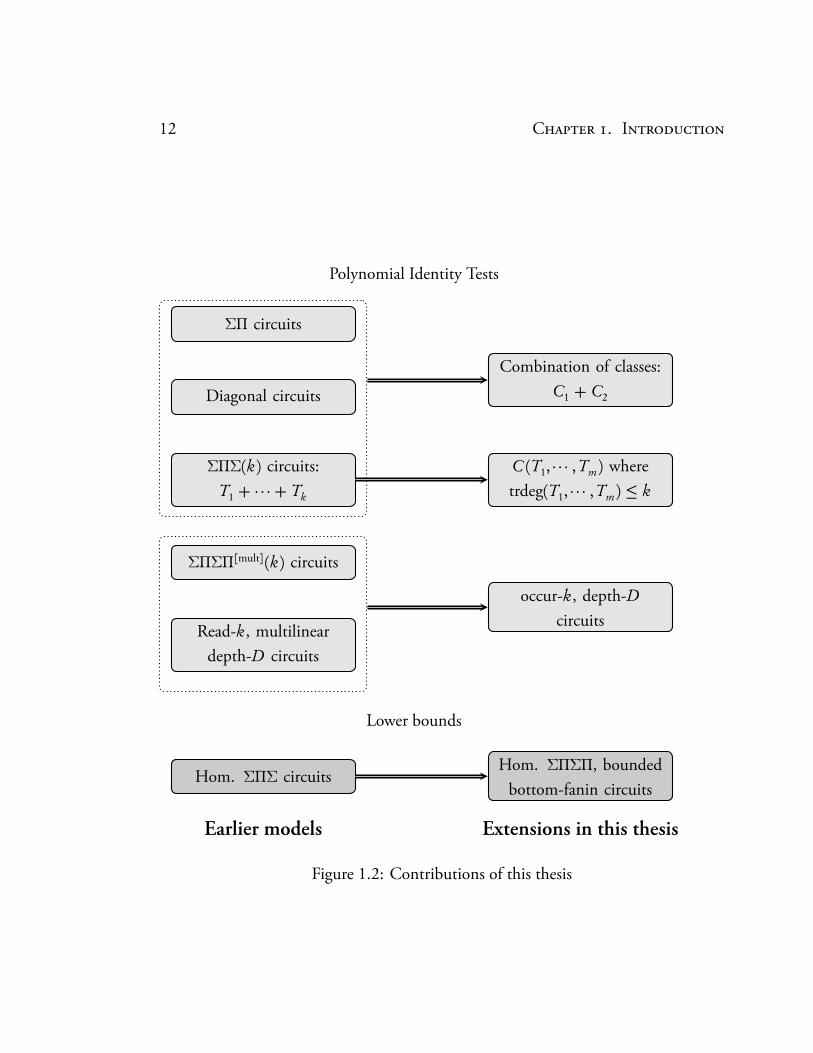
Contributions of this thesis

ough quite a lot of progress for PIT has been made for these restricted models, oneissue is the solution in each model involves a different technique tailored to work forthe models — univariate substitutions, chinese remaindering over local rings, algebraicindependence, duality transforms, shattering of partial derivatives, sparsity boundsetc. As a result, it is not clear if all these special cases throw insight into the generalproblem at all. is thesis address the following natural questions — What is thecentral core that makes PIT on these models easy? Is there a unified technique thatencompasses all these models? Can PITs of two different models be “composed” towork on “combinations” of these models? Do lower bound technique for depth-3circuits lift to larger depth?

Composition of PITs

If we know how to perform PIT on two different classes C1 and C2, can performPIT on circuits from C1 +C2? is question depends on the classes C1 and C2 ofcourse. If f is a depth-2 circuit, and g = g1 . . . gt is a product of depth-2 circuits,then checking if f = g1 . . . gt is exactly the problem of validating sparse factorization(cf. [vzG83]). e simplest models for which PITs are known are bounded fan-indepth-3 circuits and diagonal circuits. Can the two seemingly disparate techniquesglue together to give a PIT for the composed circuits? In Chapter 3, we answer thisquestion in the affirmative. Our technique also applies to a special case of the depth-4problem f −∏t

i=1 gi?= 0 where each of the gi ’s are sums of univariates.

iii

A unified technique for PITs

e next question the thesis addresses is a unification of the PITs for different models.In Chapter 4, we present a unified approach via algebraic independence and the jacobian.

We show that the Jacobian is a powerful tool to give one unified approach forblackbox PITs for all the classes for which polynomial time blackbox PITs were known,namely bounded fan-in depth-3, bounded fan-in depth-4 multilinear circuits , boundedread bounded depth multilinear circuits, and bounded transcendence degree depth-4circuits. e approach however has one caveat that the method works over all fieldswith zero or large chracteristic.

In the process of unifying the varied techniques, we strengthen the earlier resultssignificantly thus giving the first blackbox PIT for these generalized models. We con-struct blackbox PITs for not only bounded fan-in depth-3 circuits, but also for circuitsof the form C (T1, · · · ,Tm) where C is any polynomial of low degree and Ti ’s are prod-ucts of linear functions with bounded transcendence degree. Further, we remove themultilinear restriction completely from the constant-depth constant-read models. enotion of ‘read’ is also replaced by a general notion of ‘occur’, which additionally gen-eralizes PIT on ΣΠΣΠ[mult](k) circuits as well.

e connection between PIT and lowerbounds is present in this unification as well.We present lowerbounds for the Detn and Permn for almost all the models we constructPITs for, again via the Jacobian.

Approaching the chasm at depth-4

e final question addressed in this thesis is a direct attempt towards a lower boundfor the permanent. A result of Agrawal and Vinay [AV08] states that we only need toprove a strong enough lowerbound for the class of depth-4 circuits. is was subse-quently strengthened by Koiran [Koi10] to show that it suffices to prove a lower boundof exp(ω(

pn log2 n)) for homogeneous depth-4 circuit with the bottom multiplication

gates having O(p

n) fan-in to obtain super-polynomial lower bounds for general cir-cuits.

In Chapter 5 we present a lower bound of exp(Ω(p

n)) for homogeneous depth-4 circuits where the fan-in of the bottom multiplication gates having O(

pn) fan-in

that compute Detn or Permn. In the light of above results of Agrawal-Vinay [AV08]

iv

and Koiran [Koi10] that a expωp

n log2 n

lower bound suffices for a super-polynomial circuit lower bound, our result does get very close to the chasm. Fur-ther, we also exhibit that our method has the potential to show non-trivial separationsbetween the complexities of the determinant and permanent (albeit the above resultworks for both). It is conceivable that this indeed might be one of the ingredients inseparating VP and VNP.

Acknowledgements

I have been very fortunate to have Manindra Agrawal as my advisor. My stay at IITKanpur could not have been possible if not for his resourcefulness. He has helped meimmensely throughout the last several years (right from helping me move my luggageon my first day) and I feel truly indebted to him. His tenacity to focus only on funda-mental problems has been a constant source of inspiration. I hope that I can display afraction of it during the years to come.

My interest in complexity theory stemmed from the wonderful courses I had takenover the years, and my interaction with the faculty at CMI and IMSc. I’d like tothank Madhavan, Kumar, KV, Samir, Arvind, Meena and Suresh for all the coursesand discussions we’ve had. I’d specially like to thank Arvind for his wonderful courseson complexity and computational algebra that sparked my interest in this field.

I’d also like to thank the faculty at IIT Kanpur with whom I’ve interacted during mystay here. I’ve throughly enjoyed interacting with Somenath, Piyush, Sumit, Satyadev,Shashank and Surendar (and his classes were truly amazing!).

It was wonderful to work with all my collaborators, and I learnt a great deal fromeach of them. Chandan’s enthusiasm and sincerity is contagious and a big thanksto him for putting up with me for all these years. I learnt an enormous amount ofmathematics through all the collaborations with Nitin. Neeraj’s phenomenal clarityand focus has moved me deeply, and I hope to emulate his drive for concrete bigproblems in future. Many thanks to Piyush, Anindya, Ankit and Pritish as well.

I had the opportunity to make several academic visits during the term. I had anamazing time at TIFR interacting with Prahladh and Jaikumar. I wish there is a daywhen I could give a talk like Jaikumar. I’d also like to thank Madhu for hosting me atMIT. anks to Kurt Mehlhorn for the wonderful visit at MPI Saarbrücken. And abig thanks to Satya and Neeraj for the internship at MSR. e internship was the bestacademic visit I’ve ever had, and working with Neeraj was wondefully illuminating.

vi

Neeraj and Satya helped me in more ways than one, and I shall always be grateful fortheir unconditional support.

Life in IIT and CMI wouldn’t have been half as much fun if not for the company Ihad there. Many thanks to Srikanth, Nutan, Suresh, Chandan, Deepanjan, Sagarmoy,Suman, Mousumi, and Saurabh. I’d specially like to thank Srikanth and Chandanfor their lasting influence. Srikanth’s unparalleled enthusiasm for knowledge doesn’ttake too long to catch on, and I’ve learnt so much interacting with him. Chandanhas been subjected to several hours of torture by me, but ever-so-patiently answersevery question irrespective of how dumb it is. His astounding clarity in exposition issomething I hope to be capable of someday. I also feel compelled to thank Deepanjanand Suman for all the Spordha sessions.

Many thanks to my uncle, Vinay, for ... everything. He was the reason I took tomathematics and theoretical computer science in the first place, and has been an idolsince my childhood. My sincere thanks to him and Subha chitthi for everything thatI am today.

A big thank you to Susmita for sharing all my joy and pain, and life would havebeen empty without her. Most of all, thanks to my parents, my sister Kamakshi,my grandfather and grandmother for the wonderful home I grew up in. My humblenamaskarams to my grandfather specially, who would have been very proud to see this,and it is to him that I dedicate this thesis.

To my grandfather

Contents

1 Introduction 11.1 Lower Bounds . . . . . . . . . . . . . . . . . . . . . . . . . . . . . . . . . . . . 21.2 Polynomial Identity Testing . . . . . . . . . . . . . . . . . . . . . . . . . . . . 31.3 Contributions of this thesis . . . . . . . . . . . . . . . . . . . . . . . . . . . . 7

1.3.1 Composition of identity tests . . . . . . . . . . . . . . . . . . . . . 81.3.2 A unified technique for PIT . . . . . . . . . . . . . . . . . . . . . . 91.3.3 Towards lower bounds for depth-4 circuits . . . . . . . . . . . . 10

1.4 Structure of the thesis . . . . . . . . . . . . . . . . . . . . . . . . . . . . . . . . 11

2 Preliminaries 132.1 Notation . . . . . . . . . . . . . . . . . . . . . . . . . . . . . . . . . . . . . . . . 132.2 Basic tools for PIT and lower bounds . . . . . . . . . . . . . . . . . . . . . 14

2.2.1 Homogenization . . . . . . . . . . . . . . . . . . . . . . . . . . . . . 142.2.2 e Schwartz-Zippel Lemma . . . . . . . . . . . . . . . . . . . . . 152.2.3 Blackbox PIT for sparse polynomials . . . . . . . . . . . . . . . . 16

3 Composing identity tests, and sparse factorization 193.1 Introduction . . . . . . . . . . . . . . . . . . . . . . . . . . . . . . . . . . . . . 19

3.1.1 Contribution of this chapter . . . . . . . . . . . . . . . . . . . . . . 193.1.2 Overview of the approach . . . . . . . . . . . . . . . . . . . . . . . 20

3.2 PIT for semidiagonal circuits . . . . . . . . . . . . . . . . . . . . . . . . . . . 223.3 Solving Problem 3.1 . . . . . . . . . . . . . . . . . . . . . . . . . . . . . . . . 26

3.3.1 Reviewing the Kayal-Saxena test . . . . . . . . . . . . . . . . . . . 263.3.2 A brief introduction to local rings . . . . . . . . . . . . . . . . . . 273.3.3 Reviewing the Kayal-Saxena test . . . . . . . . . . . . . . . . . . . 273.3.4 Adapting Algorithm KS-Test to solve Problem 3.1 . . . . . . . 30

ix

x C

3.4 Solving Problem 3.2 . . . . . . . . . . . . . . . . . . . . . . . . . . . . . . . . 343.4.1 Checking divisibility by (a power of ) a sum of univariates . . 353.4.2 Irreducibility of a sum of univariates . . . . . . . . . . . . . . . . 363.4.3 Finishing the argument . . . . . . . . . . . . . . . . . . . . . . . . . 39

4 Identity testing via algebraic independence 414.1 Introduction . . . . . . . . . . . . . . . . . . . . . . . . . . . . . . . . . . . . . 41

4.1.1 Contribution of this chapter . . . . . . . . . . . . . . . . . . . . . . 424.1.2 e main ideas . . . . . . . . . . . . . . . . . . . . . . . . . . . . . . . 46

4.2 Algebraic independence and the Jacobian . . . . . . . . . . . . . . . . . . . 464.3 Depth-3 circuits of bounded transcendence degree . . . . . . . . . . . . . 49

4.3.1 Preserving non-zeroness of Jxk(Tk) . . . . . . . . . . . . . . . . . . 50

4.4 Constant-depth constant-occur formulas . . . . . . . . . . . . . . . . . . . 534.4.1 Restriction to the case of depth-4 . . . . . . . . . . . . . . . . . . . 554.4.2 Generalizing to larger depth . . . . . . . . . . . . . . . . . . . . . . 56

4.5 Related lower bounds . . . . . . . . . . . . . . . . . . . . . . . . . . . . . . . . 594.5.1 Lower bound on depth-4 occur-k formulas . . . . . . . . . . . . 604.5.2 Lower bound on circuits generated by ΣΠ polynomials . . . . 604.5.3 Lower bound on circuits generated by ΠΣ polynomials . . . . 614.5.4 Proofs of the technial lemmas . . . . . . . . . . . . . . . . . . . . . 62

5 Approaching the chasm at depth four 675.1 Introduction . . . . . . . . . . . . . . . . . . . . . . . . . . . . . . . . . . . . . 67

5.1.1 Prior Work . . . . . . . . . . . . . . . . . . . . . . . . . . . . . . . . . 675.1.2 e model . . . . . . . . . . . . . . . . . . . . . . . . . . . . . . . . . 68

5.2 Basic Idea and Outline . . . . . . . . . . . . . . . . . . . . . . . . . . . . . . . 695.2.1 Outline of the chapter . . . . . . . . . . . . . . . . . . . . . . . . . . 70

5.3 Shifted partials of ΣΠΣΠ[hom](t ) circuits . . . . . . . . . . . . . . . . . . . 715.4 Shifted partials of the Permanent . . . . . . . . . . . . . . . . . . . . . . . . 73

5.4.1 Restricting to two diagonals . . . . . . . . . . . . . . . . . . . . . . 745.5 Putting it all together . . . . . . . . . . . . . . . . . . . . . . . . . . . . . . . . 76

5.5.1 Growth of binomial estimates . . . . . . . . . . . . . . . . . . . . . 765.5.2 Proof of the main theorem . . . . . . . . . . . . . . . . . . . . . . . 77

C xi

5.6 Discussion . . . . . . . . . . . . . . . . . . . . . . . . . . . . . . . . . . . . . . . 79

6 Conclusion and future directions 816.1 Composing Identity tests . . . . . . . . . . . . . . . . . . . . . . . . . . . . . 816.2 PITs via algebraic independence . . . . . . . . . . . . . . . . . . . . . . . . . 826.3 Shifted partial derivatives . . . . . . . . . . . . . . . . . . . . . . . . . . . . . 83

xii C

1Introduction

Over the last few decades, research in theoretical computer science has become so-phisticated. We have acquired a variety of tools from several fields, and used themto better our understanding of computation. Several constructs from mathematicshave now become standard tools in theoretical computer science research, and the dis-tinction (if there was any) between mathematics and theoretical computer science hasbecome fuzzy.

Possibly the most basic of mathematical objects are polynomials and we would liketo understand the hardness of various natural problems concerning them. e mostrobust way to measure the hardness of the polynomial is via the number of operationsrequired to compute it, and this notion formalized via arithmetic circuits.

Definition 1.1 (Arithmetic Circuits and formulas). An arithmetic circuit is a directedacyclic graph with one sink (which is called the output gate or root). Each of the sourcevertices (which are called input nodes) are either labelled by a variable xi or an element froman underlying field F. Each of the internal nodes are labelled either by+ or× to indicate if itis an addition or multiplication gate respectively. Sometimes edges may carry weights that areelements from the field and this amounts to scaling the polynomial computed at the incomingnode by that field element.

An arithmetic circuit is a formula if every internal node has out-degree 1. e size of thecircuit/formula is the number of nodes in the graph, and the depth is the length of the longestpath from the leaf to the root.

Arithmetic circuits provide a very compact way of representing polynomials, andthis can be seen in Example 3 which has 2n terms on expanding fully. For any poly-nomial p, the size of the smallest arithmetic circuit computing it can be thought of asthe arithmetic complexity of p. We would like to know if there are explicit examples ofpolynomials that are very hard to compute, or have very large arithmetic complexity.

2 C . I

Figure 1.1: Arithmetic Circuits

..x1 . x2.

×

.

×

.

×

.

+

.

2

.

(x1+ x2)2

.

Example 1

..x1 . x2.

+

.

×

.

(x1+ x2)2

.

Example 2

..· · ·.x2 .x1 .1 . xn.

+

.

+

.

+

.

· · ·

.

×

.

(1+ x1)(1+ x2) · · · (1+ xn)

.

Example 3

1.1 Lower Bounds

Amongst the multitude of polynomials, these two are of the highest significance —the determinant and permanent polynomial (denoted by Detn and Permn respectively).

Detn =∑σ∈Sn

sign(σ) · x1σ(1) . . . xnσ(n)

Permn =∑σ∈Sn

x1σ(1) . . . xnσ(n)

Although these two polynomials look similar, they seem to be very different com-putationally. e polynomial Detn is known to be computable by arithmetic cir-cuits of polynomial size (in n) but Permn is believed to have exponential complexity.Valiant [Val79] defined the classes VP and VNP as algebraic analogues of the booleancomplexity classes P and NP. He showed that Detn was complete for VP, and Permn

was complete for VNP. Further, he showed that VP 6= VNP must necessarily be resolvedbefore showing P 6= NP. Separating the complexity of the determinant and permanentis also referred to as the determinant vs permanent conjecture, and is perhaps the mostimportant question in arithmetic complexity theory.

“e determinant of this conjecture would be permanently famous.”

– Neeraj Kayal

.. P I T 3

e current state of the art for lowerbounds for general circuits is rather bleak. Baurand Strassen [BS83] showed that any circuit computing the polynomial x r

1 + · · ·+ x rn

must have size Ω(n log r ). is is the only super-linear lowerbound known for generalcircuits. For arithmetic formulae, Kalorkoti [Kal85a] showed that any arithmetic formulacomputing Detn or Permn must have size Ω(n3).

With some additional restrictions on the circuit/formula, further lowerbounds areknown. Jerrum and Snir [JS82] showed that any monotone circuit computing Detn orPermn requires 2Ω(n) size. Raz [Raz09] showed that any multilinear circuit computingDetn or Permn requires nΩ(log n) size.

For constant depth circuits, the situation is more respectable. Grigoriev and Karpin-ski [GK98] showed that any depth-3 circuit computing Detn over finite fields musthave size 2Ω(n). But over characteristic zero fields, we only have an Ω(n4/ log n) lowerbound, due to Shpilka and Wigderson [SW01], for Detn and Permn. For homogeneousdepth-3 circuits, Nisan and Wigderson [NW97] gave a 2Ω(n) lowerbound for Detn andPermn.

All the above results do not separate the complexity of Permn from Detn. In thecontext of separation, Mignon and Ressayre [MR04] showed that the determinentalcomplexity of the Permn is Ω(n2). More formally, if one wishes to write Permn as thedeterminant of some m×m matrix with affine function entries, then m =Ω(n2).

1.2 Polynomial Identity Testing

ere are several algorithmic questions that can be asked about arithmetic circuits,and the simplest (to state) amongst them is polynomial identity testing (PIT) — givenan arithmetic circuit C as input, test if the polynomial computed by C is identicallyzero.

ough a circuit of size s can potentially compute a polynomial of degree 2s , theinput circuit for PIT is usually promised to have low degree, i.e. degree polynomiallybounded in the number of variables. is problem is sometimes referred to as low degreePIT, but throughout this thesis we will restrict ourselves to only low degree PIT andrefer to it as simply ‘PIT’. e circuit is usually assumed to be layered with alternatinglayers of + and × gates which are referred to as Σ and Π layers respectively.

ere are two types of algorithms for PIT that are studied — blackbox and non-

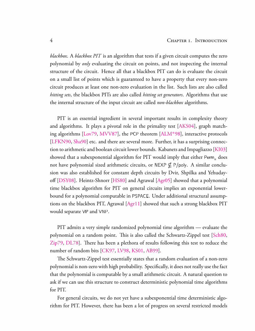
4 C . I

blackbox. A blackbox PIT is an algorithm that tests if a given circuit computes the zeropolynomial by only evaluating the circuit on points, and not inspecting the internalstructure of the circuit. Hence all that a blackbox PIT can do is evaluate the circuiton a small list of points which is guaranteed to have a property that every non-zerocircuit produces at least one non-zero evaluation in the list. Such lists are also calledhitting sets, the blackbox PITs are also called hitting set generators. Algorithms that usethe internal structure of the input circuit are called non-blackbox algorithms.

PIT is an essential ingredient in several important results in complexity theoryand algorithms. It plays a pivotal role in the primality test [AKS04], graph match-ing algorithms [Lov79, MVV87], the PCP theorem [ALM+98], interactive protocols[LFKN90, Sha90] etc. and there are several more. Further, it has a surprising connec-tion to arithmetic and boolean circuit lower bounds. Kabanets and Impagliazzo [KI03]showed that a subexponential algorithm for PIT would imply that either Permn doesnot have polynomial sized arithmetic circuits, or NEXP * P/poly. A similar conclu-sion was also established for constant depth circuits by Dvir, Shpilka and Yehuday-off [DSY08]. Heintz-Shnorr [HS80] and Agrawal [Agr05] showed that a polynomialtime blackbox algorithm for PIT on general circuits implies an exponential lower-bound for a polynomial computable in PSPACE. Under additional structural assump-tions on the blackbox PIT, Agrawal [Agr11] showed that such a strong blackbox PITwould separate VP and VNP.

PIT admits a very simple randomized polynomial time algorithm — evaluate thepolynomial on a random point. is is also called the Schwartz-Zippel test [Sch80,Zip79, DL78]. ere has been a plethora of results following this test to reduce thenumber of random bits [CK97, LV98, KS01, AB99].

e Schwartz-Zippel test essentially states that a random evaluation of a non-zeropolynomial is non-zero with high probability. Specifically, it does not really use the factthat the polynomial is computable by a small arithmetic circuit. A natural question toask if we can use this structure to construct deterministic polynomial time algorithmsfor PIT.

For general circuits, we do not yet have a subexponential time deterministic algo-rithm for PIT. However, there has been a lot of progress on several restricted models

.. P I T 5

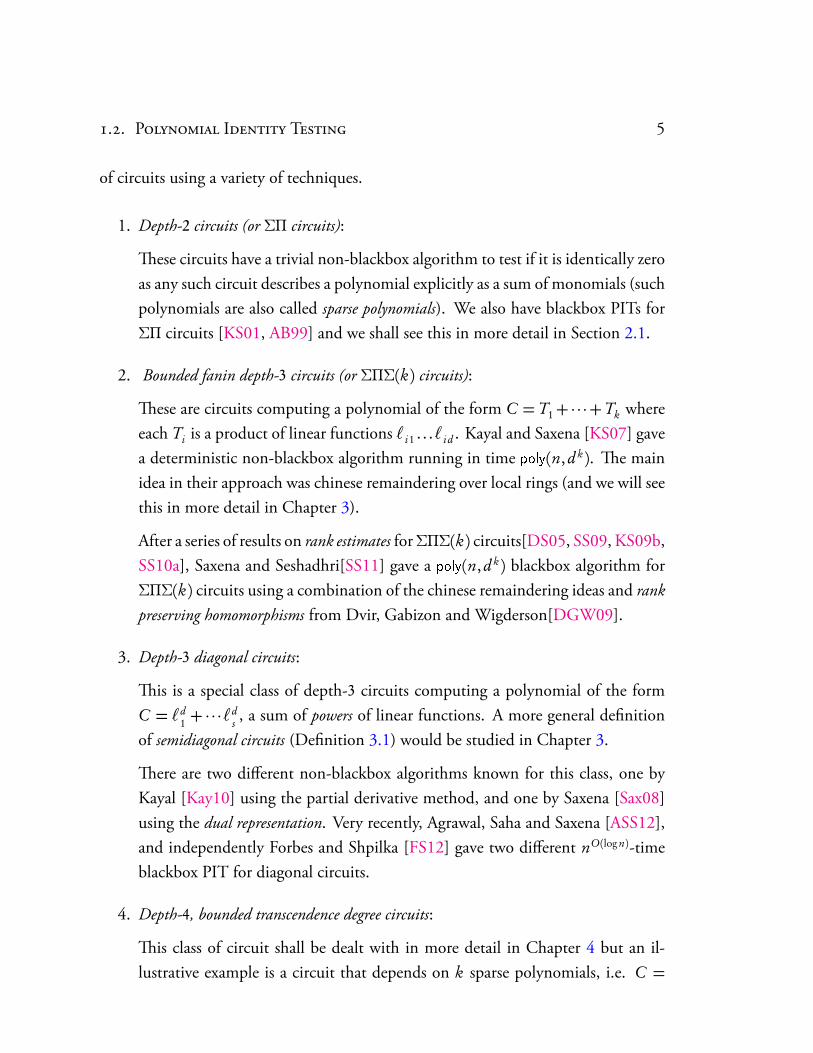
of circuits using a variety of techniques.

1. Depth-2 circuits (or ΣΠ circuits):

ese circuits have a trivial non-blackbox algorithm to test if it is identically zeroas any such circuit describes a polynomial explicitly as a sum of monomials (suchpolynomials are also called sparse polynomials). We also have blackbox PITs forΣΠ circuits [KS01, AB99] and we shall see this in more detail in Section 2.1.

2. Bounded fanin depth-3 circuits (or ΣΠΣ(k) circuits):

ese are circuits computing a polynomial of the form C = T1+ · · ·+Tk whereeach Ti is a product of linear functions `i1 . . .`i d . Kayal and Saxena [KS07] gavea deterministic non-blackbox algorithm running in time poly(n, d k). e mainidea in their approach was chinese remaindering over local rings (and we will seethis in more detail in Chapter 3).

After a series of results on rank estimates forΣΠΣ(k) circuits[DS05, SS09, KS09b,SS10a], Saxena and Seshadhri[SS11] gave a poly(n, d k) blackbox algorithm forΣΠΣ(k) circuits using a combination of the chinese remaindering ideas and rankpreserving homomorphisms from Dvir, Gabizon and Wigderson[DGW09].

3. Depth-3 diagonal circuits:

is is a special class of depth-3 circuits computing a polynomial of the formC = `d

1 + · · ·`ds , a sum of powers of linear functions. A more general definition

of semidiagonal circuits (Definition 3.1) would be studied in Chapter 3.

ere are two different non-blackbox algorithms known for this class, one byKayal [Kay10] using the partial derivative method, and one by Saxena [Sax08]using the dual representation. Very recently, Agrawal, Saha and Saxena [ASS12],and independently Forbes and Shpilka [FS12] gave two different nO(log n)-timeblackbox PIT for diagonal circuits.

4. Depth-4, bounded transcendence degree circuits:

is class of circuit shall be dealt with in more detail in Chapter 4 but an il-lustrative example is a circuit that depends on k sparse polynomials, i.e. C =

6 C . I

f (g1, · · · , gk) where f is a low-degree polynomial. Beecken, Mittman and Sax-ena [BMS11a] gave an poly(s k) blackbox PIT for this class of circuits of fieldsof zero or large characteristic. e main ingredient in their proof was algebraicindependence and the Jacobian (which would be seen in more detail in Chapter 4).

5. Depth-4, bounded fan-in, multilinear circuits (or ΣΠΣΠ[mult](k)):

A multilinear circuit is one where every gate computes a multilinear polynomial(degree of every variable is bounded by 1). Saraf and Volkovich [SV11] gave adeterministic blackbox algorithm to check if a ΣΠΣΠ[mult] circuit of top fanink is identically zero running in poly(s k3) time (where s is the size of the circuit).e main ideas used in their approach was to study the partial derivatives of thecircuit and obtain sparsity bounds on the polynomials computed by the childrenof the root.

6. Read-k, multilinear formula:

A read-k formula is one where every input variable occurs in at most k of the leafnodes. Anderson, van Melkebeek and Volkovich[AvMV11] extended the ideasin the PIT for ΣΠΣΠ[mult](k) circuits to give PITs for read-k multilinear circuits.ey give an nkO(k)-time non-blackbox PIT, and a nkO(k) log n-time blackbox PITfor this model. In the case when the depth is constant, their blackbox PIT runsin polynomial time.

e surveys by Saxena[Sax09], and by Shpilka and Yehudayoff [SY10] give wonderfulexpositions of the progress made so far in arithmetic circuit complexity.

An intriguing pattern in almost all lowerbounds and PITs stated so far is thatprogress seems to stop at depth-4. is chasm at depth-4 was ‘explained’ by Agrawal andVinay [AV08] by showing that depth-4 circuits are essentially equivalent to general cir-cuits. ey showed that any sub-exponential sized circuit computing a polynomial oflow degree can be depth-reduced to a sub-exponential sized depth-4 circuit computingthe same polynomial. e contrapositive of this theorem is that any exponential lowerbound for depth-4 circuits automatically translates to an exponential lower bound forany circuit. Agrawal and Vinay [AV08] further showed that a polynomial time black-box PIT for depth-4 circuits translates to an nO(log n)-time blackbox PIT for any general

.. C 7

circuit. In essence, they showed that ΣΠΣΠ circuits are almost as hard as general cir-cuits.

1.3 Contributions of this thesis

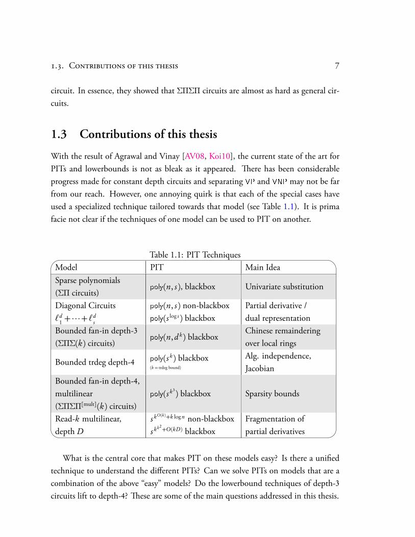
With the result of Agrawal and Vinay [AV08, Koi10], the current state of the art forPITs and lowerbounds is not as bleak as it appeared. ere has been considerableprogress made for constant depth circuits and separating VP and VNP may not be farfrom our reach. However, one annoying quirk is that each of the special cases haveused a specialized technique tailored towards that model (see Table 1.1). It is primafacie not clear if the techniques of one model can be used to PIT on another.

Table 1.1: PIT Techniques

..

Model PIT Main IdeaSparse polynomials(ΣΠ circuits)

poly(n, s ), blackbox Univariate substitution

Diagonal Circuits`d

1 + · · ·+ `ds

poly(n, s ) non-blackboxpoly(s log s ) blackbox

Partial derivative /dual representation

Bounded fan-in depth-3(ΣΠΣ(k) circuits)

poly(n, d k) blackboxChinese remainderingover local rings

Bounded trdeg depth-4 poly(s k) blackbox(k = trdeg bound)

Alg. independence,Jacobian

Bounded fan-in depth-4,multilinear(ΣΠΣΠ[mult](k) circuits)

poly(s k3) blackbox Sparsity bounds

Read-k multilinear,depth D

s kO(k)+k log n non-blackboxs kk2

+O(kD) blackboxFragmentation ofpartial derivatives

What is the central core that makes PIT on these models easy? Is there a unifiedtechnique to understand the different PITs? Can we solve PITs on models that are acombination of the above “easy” models? Do the lowerbound techniques of depth-3circuits lift to depth-4? ese are some of the main questions addressed in this thesis.

8 C . I

1.3.1 Composition of identity tests

e first question this thesis addresses is the following — suppose we know how toperform identity tests efficiently on two classes of circuits C1 and C2, how easy is it tosolve PIT on the class of circuits C1+C2? e class C1+C2 is made up of circuits C

of the form C1+C2, where C1 ∈C1 and C2 ∈C2. Depending on the classesC1 andC2,this question can be quite non-trivial to answer. For instance, suppose we are givensparse polynomials f , g1, . . . , gt , explicitly as sums of monomials, and asked to check iff =

∏ti=1 gi . Surely, it is easy to check if f or

∏ti=1 gi is zero. But, it is not clear how to

perform the test f −∏ti=1 gi

?= 0. (is problem has also been declared open in a workby [vzG83] on sparse multivariate polynomial factoring.) e test f −∏t

i=1 gi?= 0 is

one of the most basic cases of depth-4 PIT that is still open.Two of the non-trivial classes of depth-3 circuits for which efficient PIT algo-

rithms are known are the classes of bounded top fan-in [KS07] and diagonal circuits[Kay10, Sax08]. e question is - Is it possible to glue together the seemingly disparatemethods of [KS07] and [Kay10, Sax08] and give a PIT algorithm for the compositionof bounded top fan-in depth-3 and diagonal circuits, or bounded top fan-in depth-3and sparse polynomials (depth-2 circuits)? In Chapter 3, we answer this question inthe affirmative. Our technique also applies to a special case of the depth-4 problemf −∏t

i=1 gi?= 0 where each of the gi ’s are sums of univariates.

Main ideas

e key ingredient in the proof is an algorithm to identity test and compute the lead-ing monomial for a generalization of diagonal circuits and sparse polynomials calledsemidiagonal circuits (Definition 3.1).

With this in hand, the composition of PITs for ΣΠΣ(k) and sparse/diagonal circuitproceeds by a careful analysis of the Kayal-Saxena test [KS07] on the ΣΠΣ(k) partof the input, and studying the evolution of the sparse/diagonal part. e PIT forsemidiagonal circuits would help us keep the transformation of the sparse/diagonalpart in control.

To solve the problem of checking f −∏ gi?= 0 where gi ’s are sums of univariates,

we show that checking divisibility of a given polynomial f by a sum of univariatesreduces to a semidiagonal PIT. An additional result about the irreducibility of sums of

.. C 9

univariates allow us to use chinese remaindering to verify the given factorization.

1.3.2 A unified technique for PIT

e next question this thesis addresses is a quest for unification of the various tech-niques for PIT — Is there a unified approach that explains some (if not all) of theblackbox PITs on the various models? In Chapter 4 we answer this question with a“Yes!”, and the unified approach is via algebraic independence and the Jacobian intro-duced by Beecken, Mittman and Saxena [BMS11a].

We show that the Jacobian is powerful enough to give one unified approach to giveblackbox PITs for bounded fan-in depth-3, bounded fan-in depth-4 multilinear cir-cuits , bounded read bounded depth multilinear circuits, and bounded transcendencedegree depth-4 circuits of course, but with a caveat that our approach only works overfields of zero or large characteristic.

In the process of finding a universal technique, we strengthen the earlier resultssignificantly thus giving the first blackbox PIT for these generalized models. We con-struct blackbox PITs for not only bounded fan-in depth-3 circuits, but also for circuitsof the form C (T1, · · · ,Tm) where C is any polynomial of low degree and Ti ’s are prod-ucts of linear functions with bounded transcendence degree. Further, we remove themultilinear restriction completely from the constant-depth constant-read models. enotion of ‘read’ is also replaced by a general notion of ‘occur’ , which additionally gen-eralizes PIT on ΣΠΣΠ[mult](k) circuits as well.

e strong connection between PIT and lowerbounds that was alluded to earliertranslates to this unification as well. We present lowerbounds for the Detn and Permn

for almost all the models we construct PITs for, again via the Jacobian.

Main ideas

e driving question is to find out the key property that makes PIT the earlier mod-els easy, and one candidate is that some parameter for each of the models is beingbounded (depth does not qualify as such a parameter, as depth-4 is nearly as hard asthe general case [AV08]). e main contribution is to transform this boundednessinto the transcendence degree and structure of the Jacobian.

10 C . I

1.3.3 Towards lower bounds for depth-4 circuits

e final question addressed in this thesis is to push towards lowerbounds for Permn.e result of Agrawal and Vinay [AV08] states that we only need to prove a strongenough lowerbound for the class of depth-4 circuits. Koiran [Koi10] strenghtenedtheir result and showed that it suffices to prove a lower bound of exp(ω(

pn log2 n)) for

homogeneous depth-4 circuit with the bottom multiplication gates having O(p

n) fan-in to obtain super-polynomial lower bounds for general circuits. is fact of depth-4circuits almost capturing the general case is often referred to as the “chasm at depth-4”.

As mentioned in Section 1.1, there are lower bounds known for Detn and Permn

for depth-3 circuits and the main idea used is to study the rank of the partial derivativespace. Unfortunately, this technique does not scale even to the case when we have ahomogeneous circuit of the form C = T1+ · · ·+Ts with each Ti =Qi1 . . .Qi d , a productof quadratics. Is there a technique that helps us address such circuits? How close canwe get to the chasm?

In Chapter 5 we present a lower bound of exp(Ω(p

n)) for homogeneous depth-4circuits where the fan-in of the bottom multiplication gates having O(

pn) fan-in that

compute Detn or Permn. In the light of results of Agrawal-Vinay [AV08] and Koiran[Koi10] that a exp

ωp

n log2 n

lower bound would yield super-polynomial circuitlower bounds, this gets very close to the chasm.

Main ideas

e key technique in this result is to study the rank of shifted partial derivatives, orlow degree combinations of the partial derivatives. We show that that any homogeneousdepth-4 circuit with bounded bottom fan-in is weak with respect to the rank of theshifted partial derivatives. We then lowerbound the rank of the shifted partial deriva-tives of Detn, Permn by reducing it to a counting problem which we then solve.

An interesting artifact of the proof is a vague possibility of separating the complex-ity of Detn and Permn. e rank of the shifted partial derivatives is closely related to analgebraic geometric construct called the Hilbert polynomial. In the process of obtain-ing a lower bound for the rank of Detn and Permn, it turns out that certain algebraicgeometric properties of determinantal minors show that the rank of shifted partial

.. S 11

derivatives of Permn is provably larger than that of Detn. It might be possible to showthat rank of Permn is significantly larger than that of the Detn and might yield some non-trivial separation in their complexity. is measure of the rank of the shifted partialderivatives is one of the few measures that seem to visibly distinguish the complexityof the determinant and the permanent.

1.4 Structure of the thesis

Chapter 2 discusses some of the preliminaries required for the following chapters. Weshall also discuss some standard PIT/lowerbound techniques that would be useful forseveral results in the thesis. Chapter 3 deals with the question of composing iden-tity tests, and applying that to a special case of the “sparse factorization verification”problem. Chapter 4 presents the unified approach to blackbox PITs via the Jacobian.Chapter 5 is devoted to the shifted partial derivative technique and presents an exponen-tial lower bound for bounded bottom fan-in depth-4 circuits. Chapter 6 closes withsome concluding remarks, open problems and future directions.

12 C . I

....ΣΠ circuits.

Diagonal circuits

.

ΣΠΣ(k) circuits:T1 + · · · + Tk

.

ΣΠΣΠ[mult](k) circuits

.

Read-k, multilineardepth-D circuits

.

Combination of classes:C1 + C2

.

C (T1, · · · ,Tm) wheretrdeg(T1, · · · ,Tm) ≤ k

.

occur-k, depth-Dcircuits

.

Polynomial Identity Tests

.

Lower bounds

.

Hom. ΣΠΣ circuits

.

Hom. ΣΠΣΠ, boundedbottom-fanin circuits

.

Earlier models

.

Extensions in this thesis

Figure 1.2: Contributions of this thesis

2Preliminaries

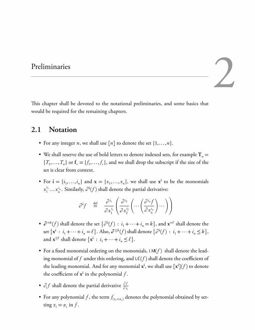
is chapter shall be devoted to the notational preliminaries, and some basics thatwould be required for the remaining chapters.

2.1 Notation

• For any integer n, we shall use [n] to denote the set 1, . . . , n.• We shall reserve the use of bold letters to denote indexed sets, for example Tn =T1, . . . ,Tn or fr = f1, . . . , fr , and we shall drop the subscript if the size of theset is clear from context.

• For i = i1, . . . , in and x = x1, . . . , xn, we shall use xi to be the monomialsx i1

1 . . . x inn . Similarly, ∂ i( f ) shall denote the partial derivative:

∂ i f def=∂ i1

∂ x i11

∂ i2

∂ x i22

· · · ∂ in f

∂ x inn

!· · ·!

• ∂ =k( f ) shall denote the set∂ i( f ) : i1+ · · ·+ in = k

, and x=` shall denote the

setxi : i1+ · · ·+ in = `

. Also, ∂ ≤k( f ) shall denote

∂ i( f ) : i1+ · · ·+ in ≤ k

,

and x≤` shall denotexi : i1+ · · ·+ in ≤ `

.

• For a fixed monomial ordering on the monomials, LM( f ) shall denote the lead-ing monomial of f under this ordering, and LC( f ) shall denote the coefficient ofthe leading monomial. And for any monomial xi, we shall use [xi]( f ) to denotethe coefficient of xi in the polynomial f .

• ∂i f shall denote the partial derivative ∂ f∂ xi

• For any polynomial f , the term f(xi=αi )denotes the polynomial obtained by set-

ting xi = αi in f .

14 C . P

• For a set of polynomials f1, . . . , fr , we shall use ⟨ f1, . . . , fr ⟩ to denote the idealgenerated by them, and ⟨ f1, . . . , fr ⟩≤` to denote the set of all `-degree combina-tions of them. at is,

⟨ f1, . . . , fr ⟩= p1 f1+ · · ·+ pr fr : pi ∈ F[x]⟨ f1, . . . , fr ⟩≤` = p1 f1+ · · ·+ pr fr : pi ∈ F[x] , deg(pi )≤ `

Polynomials and arithmetic circuits

• For a polynomial f , the sparsity of f shall denote the number of monomials inf . If the sparsity of f is polynomially bounded in the number of variables, weshall say that the polynomial f is sparse.

• A circuit/formula is said to be homogeneous if every gate computes a homo-geneous polynomial. A circuit/formula is said to be multilinear if every gatecomputes a multilinear polynomial.

• Normally, the top gate of the circuit is assumed to be a + gate (unless otherwisestated). ΣΠ shall denote the class of polynomial sized depth-2 circuits (whichare sparse polynomials). ΣΠΣ denotes of depth-3 circuits, and ΣΠΣΠ denotesthe class of depth-4 circuits. Further, we shall add the term hom or ml to denotehomogeneity or multilinearity respectively (for example, ΣΠΣΠ[hom] denotes theclass of homogeneous depth-4 circuits, and ΣΠΣΠ[hom,ml] denotes the class ofhomogeneous multilinear depth-4 circuits).

2.2 Basic tools for PIT and lower bounds

is section shall help build the some basic tools that would be required in the chaptersto follow.

2.2.1 Homogenization

In the context of PIT, the input circuit is normally assumed to be homogeneous. ereason is because of a standard trick of homogenizing a polynomial, and also homoge-nizing any circuit computing a homogeneous polynomial without too much blow-upin size.

.. B PIT 15

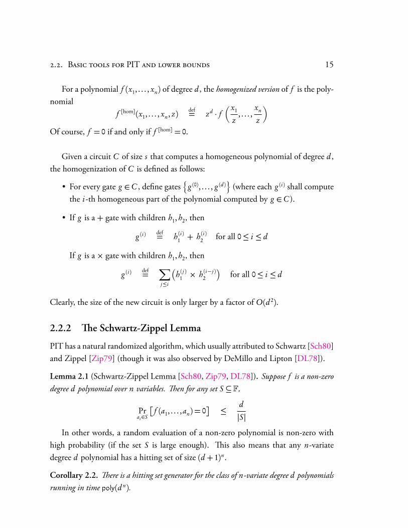
For a polynomial f (x1, . . . , xn) of degree d , the homogenized version of f is the poly-nomial

f [hom](x1, . . . , xn, z) def= zd · f x1

z, . . . ,

xn

z

Of course, f = 0 if and only if f [hom] = 0.

Given a circuit C of size s that computes a homogeneous polynomial of degree d ,the homogenization of C is defined as follows:

• For every gate g ∈C , define gates¦

g (0), . . . , g (d )©

(where each g (i) shall computethe i-th homogeneous part of the polynomial computed by g ∈C ).

• If g is a + gate with children h1, h2, then

g (i) def= h (i)1 + h (i)2 for all 0≤ i ≤ d

If g is a × gate with children h1, h2, then

g (i) def=∑j≤i

h ( j )1 × h (i− j )

2

for all 0≤ i ≤ d

Clearly, the size of the new circuit is only larger by a factor of O(d 2).

2.2.2 e Schwartz-Zippel Lemma

PIT has a natural randomized algorithm, which usually attributed to Schwartz [Sch80]and Zippel [Zip79] (though it was also observed by DeMillo and Lipton [DL78]).

Lemma 2.1 (Schwartz-Zippel Lemma [Sch80, Zip79, DL78]). Suppose f is a non-zerodegree d polynomial over n variables. en for any set S ⊆ F,

Prai∈S

f (a1, . . . ,an) = 0

≤ d

|S |In other words, a random evaluation of a non-zero polynomial is non-zero with

high probability (if the set S is large enough). is also means that any n-variatedegree d polynomial has a hitting set of size (d + 1)n.

Corollary 2.2. ere is a hitting set generator for the class of n-variate degree d polynomialsrunning in time poly(d n).

16 C . P

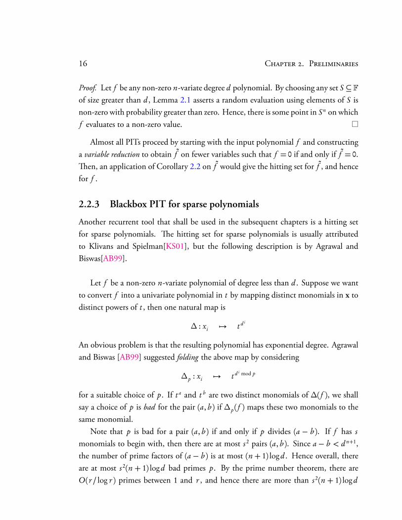
Proof. Let f be any non-zero n-variate degree d polynomial. By choosing any set S ⊆ Fof size greater than d , Lemma 2.1 asserts a random evaluation using elements of S isnon-zero with probability greater than zero. Hence, there is some point in Sn on whichf evaluates to a non-zero value.

Almost all PITs proceed by starting with the input polynomial f and constructinga variable reduction to obtain f on fewer variables such that f = 0 if and only if f = 0.en, an application of Corollary 2.2 on f would give the hitting set for f , and hencefor f .

2.2.3 Blackbox PIT for sparse polynomials

Another recurrent tool that shall be used in the subsequent chapters is a hitting setfor sparse polynomials. e hitting set for sparse polynomials is usually attributedto Klivans and Spielman[KS01], but the following description is by Agrawal andBiswas[AB99].

Let f be a non-zero n-variate polynomial of degree less than d . Suppose we wantto convert f into a univariate polynomial in t by mapping distinct monomials in x todistinct powers of t , then one natural map is

∆ : xi 7→ t d i

An obvious problem is that the resulting polynomial has exponential degree. Agrawaland Biswas [AB99] suggested folding the above map by considering

∆p : xi 7→ t d i mod p

for a suitable choice of p. If t a and t b are two distinct monomials of ∆( f ), we shallsay a choice of p is bad for the pair (a, b ) if ∆p( f ) maps these two monomials to thesame monomial.

Note that p is bad for a pair (a, b ) if and only if p divides (a − b ). If f has s

monomials to begin with, then there are at most s 2 pairs (a, b ). Since a − b < d n+1,the number of prime factors of (a − b ) is at most (n + 1) log d . Hence overall, thereare at most s 2(n + 1) log d bad primes p. By the prime number theorem, there areO(r/ log r ) primes between 1 and r , and hence there are more than s 2(n + 1) log d

.. B PIT 17

primes within the first (s 2(n+ 1) log d )2 choices of p. erefore, ∆p( f ) 6= 0 for somep ≤ (s 2(n+1) log d )2. Since ∆p( f ) has degree at most p · d , this yields this hitting set.e following lemma summarizes this discussion (with a small generalization).

Lemma 2.3. Let f1, . . . , fr be non-zero n-variate polynomials of degree less than d of sparsityat most s each. Let P = r · s 4(n+ 1)2 log2 d and S ⊆ F be any set of size greater than d · P .en, one of the elements of the following set is a point on which each fi is non-zero:¦

(α,αd mod p , . . . ,αd n−1 mod p) : α ∈ S , p ≤ P©

Proof. We shall say p is bad for fi if ∆( fi ) contains two non-zero monomials t a, t b

with p | (a− b ). As in the above discussion, the number of p’s that are bad for a singlefi is at most (s 2(n+ 1) log d )2. Hence, the number of p’s that are bad for some fi is atmost r · (s 2(n+ 1) log d )2. Hence, for some p ≤ P = r (s 2(n+ 1) log d )2, we have that∆p( fi ) 6= 0 for every i and hence F (t ) =∆p(

∏ri=1 fi ) 6= 0.

Since F (t ) is a non-zero univariate of degree at most d · P , it has at most d · P roots.Hence, for any set S ⊆ F of size greater than d · P , there is some α ∈ S such that

F (α) =r∏

i=1

fi (α,αd mod p , . . . ,αd n−1 mod p) 6= 0

which is what we wanted to show.

18 C . P

3Composing identity tests, and sparse factorization

3.1 Introduction

is chapter addresses a question on ‘composition of identity tests’ — if we know PITsfor two classesC1 andC2, can we construct PITs for circuits of the form C1+C2 whereC1 ∈C1 and C2 ∈C2? PIT on the class C1×C2 is trivial, as the product is zero if andonly if one of them is zero.

As mentioned in Chapter 1, an open problem posed by von zur Gathen [vzG83]can be thought of as such a composition problem: Given polynomial f , g1, · · · , gt

explicitly as a sum of monomials, check if

f − g1 . . . gt?= 0.

Sparse polynomials (ΣΠ circuits) are one of the simplest class of arithmetic circuits forwhich PITs are known, and following it are bounded fan-in depth-3 circuits (ΣΠΣ(k))and diagonal circuits. What can we say about the composition of these classes? Canthe seemingly different methods employed for each of these classes be used to give PITson composed circuits? is chapter answers this question in the affirmative. is alsoapplies to a special case of checking if f −∏t

i=1 gi?= 0 where each gi ’s are sums of

univariates.

3.1.1 Contribution of this chapter

is chapter presents deterministic polynomial time algorithms for two problems onidentity testing – one is on a class of depth-3 circuits, while the other is on a class ofdepth-4 circuits. As mentioned in Section 3.1, both these classes of circuits would beexamples of composition of subclasses over which we already know how to performPIT.

20 C . C

e first problem is a common generalization of the problems studied in [KS07]and [Sax08]. We shall need the following definition of a semidiagonal circuit.

Definition 3.1. (Semidiagonal circuit) Let C be a depth-3 circuit, i.e. a sum of productsof linear polynomials. e circuit is said to be an r -semidiagonal circuit if each productgate in C computes a polynomial of the form m ·∏b

i=1 `eii , where m is a monomial, `i is a

linear polynomials in the input variables and∏(1+ ei )≤ r .

Also, a term of the form (m ·∏bi=1 `

eii ) shall be called a r -semidiagonal term.

Remark. A general ΣΠΣ circuit of degree d is trivially a r -semidiagonal circuit forr = 2d but we shall be more interested in circuits where r is polynomially bounded bythe circuit size. We shall refer to such circuits as simply semidiagonal circuits (droppingthe parameter r ).

Problem 3.1. Given a depth-3 circuit C1 with bounded top fan-in and given a semidiagonalcircuit C2, test if the output of the circuit C1+C2 is identically zero.

e second problem is a special case of checking the validity of a given factorizationof a sparse multivariate polynomial (thus, a case of PIT on depth-4 top fan-in 2).

Problem 3.2. Given t + 1 polynomials f , g1, . . . , gt explicitly as sum of monomials, whereevery gi is a sum of univariate polynomials, check if f =

∏ti=1 gi .

It is possible that though f is sparse, some of its factors are not sparse (an exampleis provided in Section 3.4). So, multiplying the gi ’s in a brute force fashion is not afeasible option. In this chapter, we shall present the following:

eorem 3.2. Problem 3.1 and 3.2 can be solved in deterministic polynomial time.

3.1.2 Overview of the approach

e main tool in solving both Problem 3.1 and 3.2 is a polynomial identity test forsemidiagonal circuits.

PIT for semidiagonal circuits

ere are two known polynomial time non-blackbox PITs for semidiagonal circuits –one approach by Saxena [Sax08] using duality, and another by Kayal [Kay10] using

.. I 21

the partial derivative method. e two approaches are quite different, but both of themface a hurdle when the underlying field is of low characteristic. Saxena [Sax08]’s dual-ity can be made to work over low-characteristic fields by moving to appropriate higheralgebras, which sometimes turns out to be rather cumbersome. Kayal’s [Kay10] par-tial derivative method doesn’t work directly since derivatives of non-zero polynomialscould become zero in low characteristic fields (e.g. x p+y p). In this chapter, we presenta modification of Kayal’s [Kay10] partial derivative method that works purely on eval-uations. Further, the algorithm can be easily augmented to present an algorithm tocompute the leading monomial (and coefficient) of a given semidiagonal circuit. isadditional augmentation would turn out to be crucial in solving Problem 3.1.

e approaches to solve Problem 3.1 and 3.2 shall be described now.

Solving Problem 3.1

Let p and f be the polynomials computed by a ΣΠΣ(k) circuit and a semidiagonalcircuit respectively, and we wish to check if p + f = 0. e general idea is to applythe Kayal-Saxena test [KS07] on the polynomial p, and track the evolution of f in theprocess.

Let p = T1+ · · ·+Tk where each Ti is a product of linear forms. e original Kayal-Saxena test first chooses a T j such that LM

T j

LM (p) (recall that LM ( f ) refers tothe leading monomial of f ), and then proceeds to check if p = 0 mod T j . e purposeof this choice of T j is to ensure that p = 0 mod T j if and only if p = αT j for some α ∈ F.To apply the same test in our setting, we need to ensure that LM

T j

LM (p + f ), andhence we would require to compute LM ( f ) as well. Fortunately, the leading monomialof a semidiagonal circuit can be computed efficiently (eorem 3.6) and this lets usproceed further. e next few step of the Kayal-Saxena test employs some invertiblemaps to transform p, and this in our setting would modify f as well. By a slightlydifferent choice of a suitable invertible map, we can maintain the semidiagonal struc-ture of f . Hence, we can eventually reduce the problem of testing if p + f = 0 to asemidiagonal PIT.

22 C . C

Solving Problem 3.2

e approach to check if f =∏t

i=1 gi is quite intuitive — reduce the problem tochecking divisibility and then use chinese remaindering. But the two issues here are:how to check gi divides f , and that gi ’s need not be coprime. So in general we need tocheck if g d divides f for some d ≥ 1. We shall see that such divisibility checks reduce toidentity testing of a (slightly general) form of semidiagonal circuits. Finally, for chineseremaindering to work, we need to say something about the coprimality of gi and g j .Towards this, an irreducibility result on polynomials of the form f (x) + g (y) + h(z)would help us conclude the proof (in Section 3.4).

3.2 PIT for semidiagonal circuits

e main result of this section would be a deterministic polynomial time algorithm tosolve a stronger problem of computing F-linear dependencies for semidiagonal circuits.

Definition 3.3. (F-linear dependencies) Let f(X) =

f1(X), . . . , fm(X) ∈ (F[X])m be a

vector of polynomials. e set of F-linear dependencies of these polynomials, denoted by f⊥,is defined as

f⊥ =¦(a1, . . . ,am) ∈ Fm :

∑ai fi = 0

©Since f⊥ forms a vector space, we can talk about computing a basis of this vector

space in polynomial time. e computational problem of obtaining a basis of f⊥ givenf is referred to as PD(f) (studied in great detail in [Kay10] where it was firstintroduced).

Just like polynomial identity testing, PD also admits a randomized polyno-mial time algorithm when the polynomials in the input vector is presented as circuits.It is also known that PIT testing reduces to PD via turing reductions but is un-clear they are equivalent. Kayal [Kay10] showed that PD of semidiagonal termscan be computed in deterministic polynomial time over fields of zero or large charac-teristic, by exploiting the structure of partial derivatives. In this section, using slightmodification, we will adapt the algorithm of Kayal [Kay10] to compute PD overarbitrary fields (or finite dimensional algebras over fields) of large enough size.

To proceed with the algorithm, we shall need the following two simple lemmas.

.. PIT 23

Lemma 3.4. Let f(X) def= ( f1(X), . . . , fm(X)) ∈ (F[X])m be a vector of polynomials each ofwhose x1-degree is bounded by d . en, for any (d + 1) distinct scalars α1, . . . ,αd+1 ∈ F,

f⊥ =d+1∩i=1

f(x1=αi )

⊥where by f(x1=αi )

shall denote the vector of polynomials obtained by substituting x1 = αi ineach of its coordinates.

Proof. Of course, any vectora1, · · · ,am

satisfying

∑ai fi = 0 would also satisfy the

equation∑

ai f(x1=α)= 0 for any α. Hence, it is clear that f⊥ is contained in the RHS. As

for the other direction, consider any (a1, . . . ,am) that is not contained in f⊥. e linearcombination

∑ai fi can be thought of as a non-zero polynomial in x1 with coefficients

as polynomials in the other variables. Since the degree is bounded by d , there can beat most d roots to this polynomial. Hence (a1, . . . ,am) is not in

f(x1=αi )

⊥for some

1≤ i ≤ d + 1.

Lemma 3.5. [Kay10] Let f1, . . . , fm ∈ F[x1, . . . , xn]. Suppose h1, . . . , ht ∈ F[x1, . . . , xn]such that for every i , there is some bi

def= (bi1, . . . , bi t ) ∈ Ft such that

fi = bi1h1+ · · ·+ bi t ht

Given a basis for h⊥ and the vectors bi , we can compute f⊥ in deterministic polynomial time.

Proof. Given a basis for h⊥, we can compute a basis h1, . . . , hr that are linearly inde-pendent and rewrite every other hi as linear combination of h1, . . . , hr . erefore,each fi can be rewritten in this basis as well, i.e.,

fi = ci1h1+ . . . ci r hr where ci j ∈ F.It follows that f⊥ is just

ci1, . . . , ci r

: i = 1, . . . , m

⊥ as h1, . . . , hr are linearly inde-pendent.

We are now ready to state and prove the main theorem of this section.

eorem 3.6 (Semidiagonal PIT). Given an r -semidiagonal circuit C (over n variablesand degree d ) of the form

C =s∑

i=1

αi ·mi

b∏j=1

`ei j

i j , αi ∈ F

24 C . C

we can test in deterministic poly(s , n, d , r ) time if C is identically zero. Further, if C isnot identically zero, we can compute the leading monomial and coefficient induced by thelexicographic ordering on the variables.

Proof. We shall in fact present a polynomial time algorithm for PD on a given setof semidiagonal terms. It is clear that checking if C is identically zero is equivalent to

checking if (α1, . . . ,αs ) is contained inn

mi∏b

j=1 `e j

i j

o⊥. It would be useful to perform

a one-time ‘saturation’ of the set of semidiagonal terms to the following set S definedas

S def=

mi

b∏j=1

`e ′i j

i j : i = 1, . . . , s and 1≤ e ′i j ≤ ei j

.

Note that |S | ≤ maxi

∏bj=1(1+ ei j )

· s and this is bounded by s · r . e reason for

this saturation is because this gives us a handle on how terms evolve under partialevaluations. For any f ∈ S and α ∈ F, we can write f(x1=α)

as a linear combination ofthe polynomials in

S1 =

(mi )(x1=1)

b∏j=1

`e ′i j

i j

(x1=0)

: i = 1, . . . , s and 0≤ e ′i j ≤ ei j

.

Further, these linear combinations can be efficiently computed given α and C by sim-ply expanding using the binomial expansion. Observe that the size of S1 is at most thesize of S, but every element of S1 is semidiagonal term over (n−1) variables. is leadsto a natural recursive algorithm for PD(S) using Lemma 3.4 and Lemma 3.5.

1. If n = 0, the elements of S are just scalars and the problem is trivial.

2. Otherwise, pick distinct α1, . . . ,αd+1 ∈ F. For each f ∈ S and i = 1, . . . , (d + 1),write f(x1=αi )

as a linear combination of elements in S1.

3. Recursively compute PD(S1), a basis for the set of dependencies of S1.

4. From PD(S1) (using Lemma 3.5), compute a basis of dependencies for

Vi =¦

f(x1=αi ): f ∈ S

©⊥for each i = 1, . . . , (d + 1).

.. PIT 25

5. Return a basis for

S⊥ =d+1∩i=1

Vi (by Lemma 3.4)

e correctness of the algorithm is clear from Lemma 3.4 and Lemma 3.5. As forthe time complexity analysis, notice that every step besides Step 3 can be computedin poly(n, d , |S |) time. And Step 3 is a recursive call to PD on polynomials over(n−1) variables, and the size of S1 is no larger than the size of S. Hence, if T (n, d , |S |)denotes the time complexity of PD, we have:

T (n, d , |S |) = T (n− 1, d , |S |) + poly(n, d , |S |)=⇒ T (n, d , |S |) = poly(n, d , |S |) = poly(n, d , r, s)

Computing the leading monomial: e coefficient of any degree d univariate poly-nomial f (x1) can be interpolated (d + 1) evaluations. Formally, if [x i

1] f denotes thecoefficient of x i

1 in f , for every α1, . . . ,αd+1 ∈ F, there exists β1, . . . ,βd+1 ∈ F such that

[x i1] f = β1 f(x1=α1)

+ · · ·+βd+1 f(x1=αd+1)

In the case when f is a semidiagonal circuit (interpretting it as a univariate in x1 withcoefficients in the remaining variables), the RHS is a linear combination of semidiag-onal terms. Hence, we have a natural algorithm to compute the leading monomial off under the lexicographic order.

1. If n = 0, then f is a scalar and the problem is trivial.

2. Otherwise, compute the largest i for which

[x i1] f = β1 f(x1=α1)

+ · · ·+βd+1 f(x1=αd+1)6= 0

If no such i exists, return Z. Else, recursively compute the leading mono-mial and coefficient of [x i

1] f and return LM ( f ) = x i1 · LM

[x i

1] f

and LC ( f ) =LC[x i

1] f.

e correctness of the algorithm is obvious and the time complexity is poly(n, d , r, s )as earlier.

26 C . C

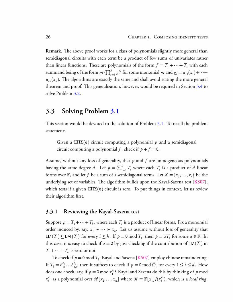
Remark. e above proof works for a class of polynomials slightly more general thansemidiagonal circuits with each term be a product of few sums of univariates ratherthan linear functions. ese are polynomials of the form f = T1+ · · ·+Ts with eachsummand being of the form m ·∏b

i=1 g eii for some monomial m and gi = ui1(x1)+· · ·+

ui n(xn). e algorithms are exactly the same and shall avoid stating the more generaltheorem and proof. is generalization, however, would be required in Section 3.4 tosolve Problem 3.2.

3.3 Solving Problem 3.1

is section would be devoted to the solution of Problem 3.1. To recall the problemstatement:

Given a ΣΠΣ(k) circuit computing a polynomial p and a semidiagonalcircuit computing a polynomial f , check if p + f = 0.

Assume, without any loss of generality, that p and f are homogeneous polynomialshaving the same degree d . Let p =

∑ki=1 Ti where each Ti is a product of d linear

forms over F, and let f be a sum of s semidiagonal terms. Let X = x1, . . . , xn be theunderlying set of variables. e algorithm builds upon the Kayal-Saxena test [KS07],which tests if a given ΣΠΣ(k) circuit is zero. To put things in context, let us reviewtheir algorithm first.

3.3.1 Reviewing the Kayal-Saxena test

Suppose p = T1+ · · ·+Tk , where each Ti is a product of linear forms. Fix a monomialorder induced by, say, x1 · · · xn. Let us assume without loss of generality thatLM (T1) LM

Ti

for every i ≤ k. If p = 0 mod T1, then p = αT1 for some α ∈ F. In

this case, it is easy to check if α = 0 by just checking if the contribution of LM (T1) inT1+ · · ·+Tk is zero or not.

To check if p = 0 mod T1, Kayal and Saxena [KS07] employ chinese remaindering.If T1 = `

e111 . . .`ed

1d, then it suffices to check if p = 0 mod `ei

1i for every 1 ≤ i ≤ d . Howdoes one check, say, if p = 0 mod x e1

1 ? Kayal and Saxena do this by thinking of p mod

x e11 as a polynomial over R[x2, . . . , xn] where R = F[x1]/(x

e11 ), which is a local ring.

.. S P . 27

ey show that the essential ideas and chinese remaindering continues to work oversuch local rings. Before we proceed to the algorithm of Kayal and Saxena, we shallspend some time understanding the basic properties of local rings that we shall require.

3.3.2 A brief introduction to local rings

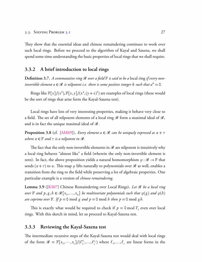
Definition 3.7. A commutative ringR over a field F is said to be a local ring if every non-invertible element a ∈R is nilpotent i.e. there is some positive integer k such that ak = 0.

Rings like F[x]/(x5),F[x, y]/(x4, (y+ x)3) are examples of local rings (these wouldbe the sort of rings that arise form the Kayal-Saxena test).

Local rings have lots of very interesting properties, making it behave very close toa field. e set of all nilpotent elements of a local ring R form a maximal ideal of R ,and is in fact the unique maximal ideal of R .

Proposition 3.8 (cf. [AM69]). Every element a ∈ R can be uniquely expressed as α+ τwhere α ∈ F and τ is a nilpotent inR .

e fact that the only non-invertible elements inR are nilpotent is intuitively whya local ring behaves “almost like” a field (wherein the only non-invertible element iszero). In fact, the above proposition yields a natural homomorphism ϕ :R → F thatsends (α+τ) to α. is map ϕ lifts naturally to polynomials overR as well, enables atransition from the ring to the field while preserving a lot of algebraic properties. Oneparticular example is a version of chinese remaindering.

Lemma 3.9 ([KS07] Chinese Remaindering over Local Rings). Let R be a local ringover F and p, g , h ∈ R[x1, . . . , xn] be multivariate polynomials such that ϕ(g ) and ϕ(h)are coprime over F. If p = 0 mod g and p = 0 mod h then p = 0 mod g h.

is is exactly what would be required to check if p = 0 mod T1 even over localrings. With this sketch in mind, let us proceed to Kayal-Saxena test.

3.3.3 Reviewing the Kayal-Saxena test

e intermediate recursive steps of the Kayal-Saxena test would deal with local ringsof the form R = F[x1, · · · , xc]/(`

e11 , . . . ,`ec

c ) where `1, . . . ,`c are linear forms in the

28 C . C

variables x1, . . . , xc . Note that dimFR ≤ d c where d is an upper-bound on the ei ’s. Weshall refer to the rest of the variables

xc+1, . . . , xn

as the free variables. Note that any

F-linear combination of x1, . . . , xn, when thought of as an element of R[xc+1, . . . , xn],can be expressed as a sum `+τ where ` is a polynomial over the free variables and τ is anilpotent inR . e following Algorithm KS-Test would take as input the descriptionofR specified by the relations

¦`e1

1 , . . . ,`ecc

©, products of linear functions T1, · · · ,Tk ′

and test if p = T1+ · · ·+Tk ′ is zero or not. To begin with, R = F, c = 0, k ′ = k andp = p. e invariant that shall be maintained is that c + k ′ ≤ k.

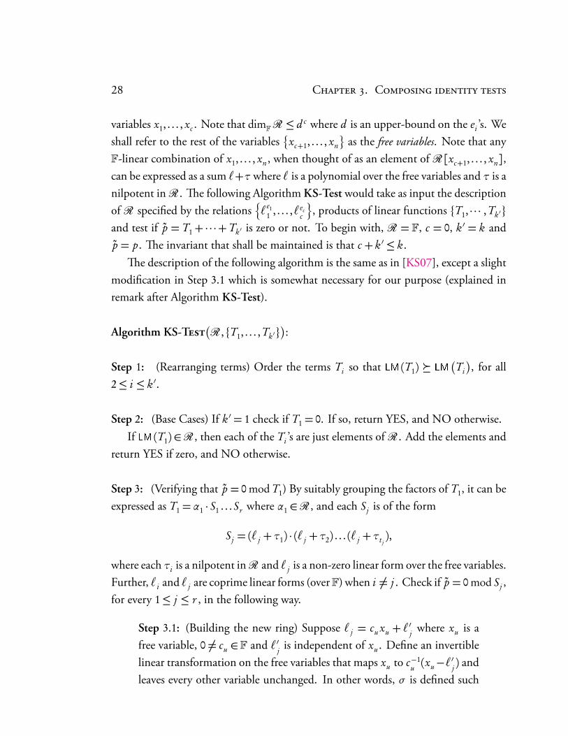
e description of the following algorithm is the same as in [KS07], except a slightmodification in Step 3.1 which is somewhat necessary for our purpose (explained inremark after Algorithm KS-Test).

Algorithm KS-TR ,T1, . . . ,Tk ′

:

Step 1: (Rearranging terms) Order the terms Ti so that LM (T1) LMTi

, for all

2≤ i ≤ k ′.

Step 2: (Base Cases) If k ′ = 1 check if T1 = 0. If so, return YES, and NO otherwise.If LM (T1) ∈R , then each of the Ti ’s are just elements ofR . Add the elements and

return YES if zero, and NO otherwise.

Step 3: (Verifying that p = 0 mod T1) By suitably grouping the factors of T1, it can beexpressed as T1 = α1 · S1 . . . Sr where α1 ∈R , and each S j is of the form

S j = (` j +τ1) · (` j +τ2) . . . (` j +τt j),

where each τi is a nilpotent inR and ` j is a non-zero linear form over the free variables.Further, `i and ` j are coprime linear forms (overF) when i 6= j . Check if p = 0 mod S j ,for every 1≤ j ≤ r , in the following way.

Step 3.1: (Building the new ring) Suppose ` j = cu xu + `′j where xu is a

free variable, 0 6= cu ∈ F and `′j is independent of xu . Define an invertiblelinear transformation on the free variables that maps xu to c−1

u (xu−`′j ) andleaves every other variable unchanged. In other words, σ is defined such

.. S P . 29

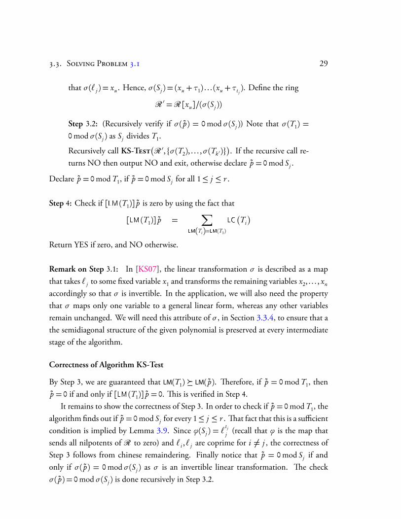
that σ(` j ) = xu . Hence, σ(S j ) = (xu +τ1) . . . (xu +τt j). Define the ring

R ′ =R[xu]/(σ(S j ))

Step 3.2: (Recursively verify if σ( p) = 0 mod σ(S j )) Note that σ(T1) =0 mod σ(S j ) as S j divides T1.

Recursively call KS-TR ′,σ(T2), . . . ,σ(Tk ′)

. If the recursive call re-

turns NO then output NO and exit, otherwise declare p = 0 mod S j .

Declare p = 0 mod T1, if p = 0 mod S j for all 1≤ j ≤ r .

Step 4: Check if [LM (T1)] p is zero by using the fact that

[LM (T1)] p =∑

LM(Ti)=LM(T1)

LCTi

Return YES if zero, and NO otherwise.

Remark on Step 3.1: In [KS07], the linear transformation σ is described as a mapthat takes ` j to some fixed variable x1 and transforms the remaining variables x2, . . . , xn

accordingly so that σ is invertible. In the application, we will also need the propertythat σ maps only one variable to a general linear form, whereas any other variablesremain unchanged. We will need this attribute of σ , in Section 3.3.4, to ensure that athe semidiagonal structure of the given polynomial is preserved at every intermediatestage of the algorithm.

Correctness of Algorithm KS-Test

By Step 3, we are guaranteed that LM(T1) LM( p). erefore, if p = 0 mod T1, thenp = 0 if and only if [LM (T1)] p = 0. is is verified in Step 4.

It remains to show the correctness of Step 3. In order to check if p = 0 mod T1, thealgorithm finds out if p = 0 mod S j for every 1≤ j ≤ r . at fact that this is a sufficientcondition is implied by Lemma 3.9. Since ϕ(S j ) = `

t j

j (recall that ϕ is the map thatsends all nilpotents of R to zero) and `i ,` j are coprime for i 6= j , the correctness ofStep 3 follows from chinese remaindering. Finally notice that p = 0 mod S j if andonly if σ( p) = 0 mod σ(S j ) as σ is an invertible linear transformation. e checkσ( p) = 0 mod σ(S j ) is done recursively in Step 3.2.

30 C . C

Complexity of Algorithm KS-Test

At the start, Algorithm KS-Test is called on polynomial p. So, at every intermediatelevel deg(S j )≤ deg(T1)≤ d . erefore, dimF(R ′)≤ d · dimF(R). Time spent by Algo-rithmKS-Test is bounded by poly(n, k ′, d , dimF(R)) in Steps 1, 2, 3.1 and 4. Moreover,time spent in Step 3.2 is at most d times a smaller problem (with top fan-in reducedby 1) while dimension of the underlying local ring gets raised by a factor at most d .Unfolding the recursion, we get the time complexity of Algorithm KS-Test on inputp to be poly(n, d k).

3.3.4 Adapting Algorithm KS-Test to solve Problem 3.1

We now wish to identity test a polynomial of the form p + f where p is computedby a ΣΠΣ(k) and f is an r -semidiagonal circuit (cf. Definition 3.1). ough p + f

is a ΣΠΣ circuit, it is a ΣΠΣ circuit of unbounded top fan-in and hence we can notapply the Kayal-Saxena test directly. We shall apply the test on p, which is a fanin-k depth-3 circuit, and track the evolution of f in the process. We shall see that thesemidiagonal structure of f is preserved throughout the execution. To begin with, f

an r -semidiagonal circuit.Just as in the Kayal-Saxena test, an intermediate level of the recursion would involve

a local ring R = F[x1, . . . , xc]/(`e11 , . . . ,`ec

c ). As before, we shall refer to the variablesxc+1, . . . , xn

as the free variables. But now, we have to test if a polynomial of the form

q =k ′∑

i=1

Ti +s ′∑

t=1

ωt

is zero where each Ti is a product of linear forms and each ωt is an r -semidiagonalterm. Each of the Ti ’s, like earlier, can be expressed as Ti = αi ·∏d

j=1(`i j +τi j ) forsome αi ∈ R , linear forms `i j over the free variables, and nilpotents τi j ∈ R . Andeach ωt is an r ′-semidiagonal term that can be written as

ωt = βt ·mt

b∏i=1

(`i t +τi t )ei t (3.1)

where mt is a monomial in the free variables and βt ∈ R . Let p denote the partT1 + · · ·+ Tk ′ , and let f denote the part

∑s ′t=1ωt . e polynomials p and f are the

.. S P . 31

evolutions of p and f in the course of the algorithm. At the beginning p = p andf = f , and the algorithm shall maintain the invariant that c + k ′ ≤ k and r ′ ≤ d c · r ,which would ensure that f stays semidiagonal.

In this modification, we would need to compute the leading monomial and co-efficient of f as well. We know from eorem 3.6 that we can compute the leadingmonomial and coefficient of a semidiagonal polynomial over F, but here f is a semidi-agonal polynomial over a local ringR . e same approach, with minor modifications,can be used to compute the leading monomial and coefficient of f as well, but we shalldefer that to later. For now let us assume that we know how to compute LM

f

and

LC

f. Below is the modified algorithm, with the changes from Algorithm KS-Test

marked.

Algorithm KS-T-MR ,T1, . . . ,Tk ′ , f

:

Step 1: (Rearranging terms) Order the terms Ti so that LM (T1) LMTi

, for all

2≤ i ≤ k ′.

Step 1.1: If LM( f ) LM (T1), return NO.

Step 2: (Base Cases) If f = 0, return KS-TestR ,T1, . . . ,Tk ′

. If k ′ = 0 check if

f = 0. If so, return YES, and NO otherewise.If LM (T1) ∈ R , then each of the Ti ’s and f are just elements of R . Add the ele-

ments and return YES if zero, and NO otherwise.

Step 3: (Verifying that p + f = 0 mod T1) By suitably grouping factors of T1, it canbe written as T1 = α1 · S1 . . . Sm where α1 ∈R , and each S j is of the form

S j = (` j +τ1) · (` j +τ2) . . . (` j +τt j),

where each τi is a nilpotent inR and ` j is a non-zero linear form over the free variables.Further, `i and ` j are coprime linear polynomials (over F) when i 6= j . Check ifp + f = 0 mod S j , for every 1≤ j ≤ m, in the following way.

Step 3.1: (Building the new ring) Suppose ` j = cu xu + `′j where xu is a

free variable, 0 6= cu ∈ F and `′j is independent of xu . Define an invertible

32 C . C

linear transformation on the free variables that maps xu to c−1u (xu−`′j ) and

leaves every other variable unchanged. In other words, σ is defined suchthat σ(` j ) = xu . Hence, σ(S j ) = (xu +τ1) . . . (xu +τt j

). Define the ring

R ′ =R[xu]/(σ(S j ))

Step 3.2: (Recursively verify if σ( p + f ) = 0 mod σ(S j )) Notice that wehave σ(T1) = 0 mod σ(S j ) as S j divides T1.

Recursively call KS-T-MR ′,¦σ(T2), . . . ,σ(T

′k ′)©

,σ( f ). Re-

turn NO if the call returns NO, otherwise declare p + f = 0 mod S j .

Declare p + f = 0 mod T1, if p + f = 0 mod S j for all 1≤ j ≤ m.

Step 4: Check if [LM (T1)]( p + f ) = 0 using the fact that

[LM (T1)]( p + f ) =

∑LM(Ti)=LM(T1)

LCTi

if LM( f )≺ LM (T1)

LC( f ) +∑

LM(Ti)=LM(T1)

LCTi

otherwise

Return YES if zero, and NO otherwise.

Correctness of Algorithm KS-Test-Modified

Recall that in Step 1 of Algorithm KS-Test, we rearranged terms to have LM (T1) LMTi

for all 2≤ i ≤ k ′. e purpose of this step was to ensure that LM (T1) LM ( p),

so that p = 0 mod T1 implies that p = α · T1 for some α ∈ R . Since we are nowdealing with p + f , we need to account for the contribution of f as well. Note thatif LM( f ) LM

Ti

for all 1 ≤ i ≤ k ′ then surely p + f 6= 0. Otherwise, T1 (after

reordering) satisfies LM (T1) LM ( p) and we can proceed to Step 2. is is preciselywhat is checked in Step 1.1 of the modified algorithm. erefore if p+ f = 0 mod T1,then p + f = α ·T1, and this is checked in Step 3. Note that Step 1.1 ensures that, inStep 3, we just have to check if p+ f = 0 mod T1 rather than p+ f = 0 mod f (which,presumably, is a much harder task).

.. S P . 33

Step 2 of the modified algorithm also handles the base case when k = 0, where wehave to check if f = 0 in R .

Step 3 remains the same as before, and the only property that needs to be ensuredis that σ( f ) continues to stay semidiagonal. Note that the choice of σ ensures that atmost one new free variable is mapped to a linear form (Step 3.2 only replaces xu , andother variables remain unchanged). erefore, σ( f ) is a sum of the terms σ(ωt )’s, andeach σ(ωt ) has at most one power of a linear form more than ωt . In other words, iff is r ′-semidiagonal, then σ( f ) is d r ′-semidiagonal. Again Lemma 3.9 ensures thatp + f = 0 mod S j for all 1≤ j ≤ m implies p + f = 0 mod T1.

Finally, in Step 4, we need to confirm if [LM (T1)]( p+ f ) = 0. Since we have ensuredin Step 1.1 that LM( f ) LM (T1), Step 4 of the modified algorithm additional accountsfor the contribution of f to the sum depending on whether LM( f ) = LM (T1) or not.

Also note that to begin with k ′ = k, c = 0 , and r ′ = r . And in each recursivestage of the algorithm, c increases by at most one, r ′ increases by a factor of d and k ′

decreases by 1. Hence, we always have that c + k ′ ≤ k and r ′ ≤ r d c ≤ d k .We now shall see how the leading monomial and coefficient of f can be computed.

Computing LM

f- From Equation 3.1

f =s ′∑

t=1

ωt

where each ωt = βt ·mt ·b ′∏

i=1

(`i t +τi t )ei t

By using the binomial expansion on (`i t + τi t )ei t , we can express f as an R-linear

combination of semidiagonal terms (reusing symbols βt ’s):

f =∑t≤s ′

e ′i t≤ei t

βt ·mt ·b ′∏

i=1

`e ′i ti t (3.2)

Note that each `i t is a linear form over the base field F, and hence the above expres-sion is a R-linear combination of semidiagonal terms over F. Also, the number ofsummands in the above expression of f is at most r ′ s ′ since f is r ′-semidiagonal.

34 C . C

Let v1, . . . , vdimFR be an F-basis of R and let each βi be expressed in this basis as

βi =∑

j

bi j v j where bi j ∈ F.

en, Equation (3.2) can be split in terms of these basis vectors as follows:

If f jdef=

∑t≤s ′

e ′i t≤e ′i t

bt j ·mt

b ′∏i=1

`ei ti t for j = 1, . . . , dimFR

then f =dimFR∑

j=1

v j · f j

us to compute the leading monomial (or coefficient) of f , it suffices to computethe leading monomial (or coefficient) of each of the f j ’s which are semidiagonal cir-cuits over F. Hence, the leading monomial and coefficient of f can be computed indeterministic poly(n, d , r ′, s ′, dimFR) time by (dimF(R))-many applications of eo-rem 3.6.

Using an analysis similar to the complexity analysis of Algorithm KS-Test (pre-sented in Section 3.3.3) and observing that dimFR ≤ d k , we see that Algorithm KS-Test-Modified takes time poly(n, r, s , d k). is solves Problem 3.1 in deterministicpolynomial time as promised. Summarizing this as a theorem:

eorem 3.10. Given aΣΠΣ(k) circuit computing a polynomial p, and an r -semidiagonalcircuit computing a polynomial f , there is a deterministic poly(n, r, s , d k)-time algorithm tocheck if p + f = 0.

3.4 Solving Problem 3.2

is section shall address Problem 3.2, a special case of “sparse factorization verifica-tion”:

Given polynomials f , g1, · · · , gt explicitly as a sum of monomial with eachgi being a sum of univariates, check if f − g1 . . . gt = 0.

e naïve approach of multiplying all gi ’s is infeasible because of intermediate swellingin the number of monomials (as sparse polynomials could have factors of very large

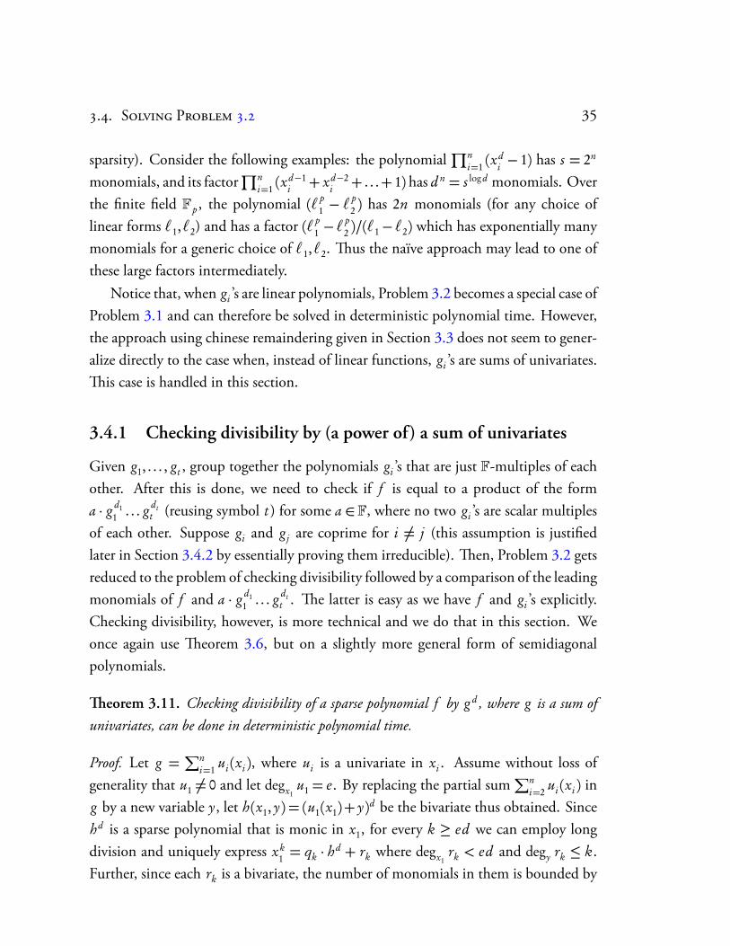
.. S P . 35

sparsity). Consider the following examples: the polynomial∏n

i=1 (xdi − 1) has s = 2n

monomials, and its factor∏n

i=1 (xd−1i + xd−2

i + . . .+ 1) has d n = s log d monomials. Overthe finite field Fp , the polynomial (`p

1 − `p2 ) has 2n monomials (for any choice of

linear forms `1,`2) and has a factor (`p1 − `p

2 )/(`1− `2) which has exponentially manymonomials for a generic choice of `1,`2. us the naïve approach may lead to one ofthese large factors intermediately.

Notice that, when gi ’s are linear polynomials, Problem 3.2 becomes a special case ofProblem 3.1 and can therefore be solved in deterministic polynomial time. However,the approach using chinese remaindering given in Section 3.3 does not seem to gener-alize directly to the case when, instead of linear functions, gi ’s are sums of univariates.is case is handled in this section.

3.4.1 Checking divisibility by (a power of) a sum of univariates

Given g1, . . . , gt , group together the polynomials gi ’s that are just F-multiples of eachother. After this is done, we need to check if f is equal to a product of the forma · g d1

1 . . . g dtt (reusing symbol t ) for some a ∈ F, where no two gi ’s are scalar multiples

of each other. Suppose gi and g j are coprime for i 6= j (this assumption is justifiedlater in Section 3.4.2 by essentially proving them irreducible). en, Problem 3.2 getsreduced to the problem of checking divisibility followed by a comparison of the leadingmonomials of f and a · g d1

1 . . . g dtt . e latter is easy as we have f and gi ’s explicitly.

Checking divisibility, however, is more technical and we do that in this section. Weonce again use eorem 3.6, but on a slightly more general form of semidiagonalpolynomials.

eorem 3.11. Checking divisibility of a sparse polynomial f by g d , where g is a sum ofunivariates, can be done in deterministic polynomial time.

Proof. Let g =∑n

i=1 ui (xi ), where ui is a univariate in xi . Assume without loss ofgenerality that u1 6= 0 and let degx1

u1 = e . By replacing the partial sum∑n

i=2 ui (xi ) ing by a new variable y, let h(x1, y) = (u1(x1)+ y)d be the bivariate thus obtained. Sincehd is a sparse polynomial that is monic in x1, for every k ≥ ed we can employ longdivision and uniquely express xk

1 = qk · hd + rk where degx1rk < ed and degy rk ≤ k.

Further, since each rk is a bivariate, the number of monomials in them is bounded by

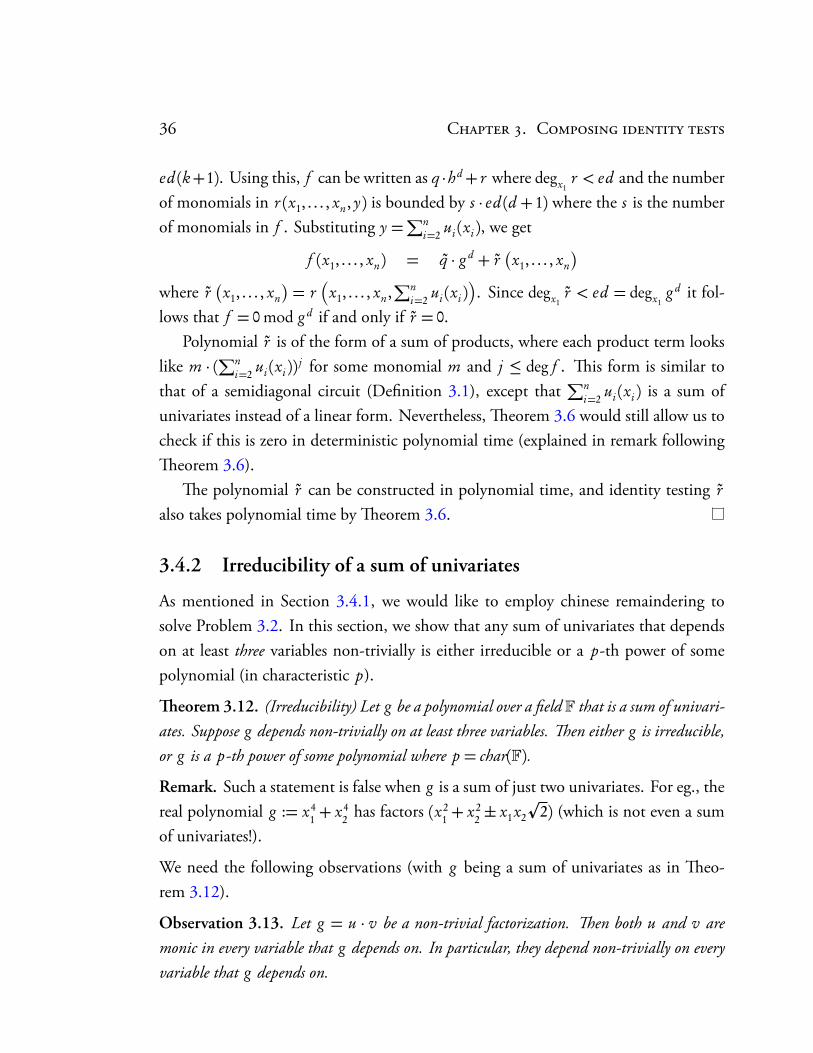
36 C . C

ed (k+1). Using this, f can be written as q ·hd+ r where degx1r < ed and the number

of monomials in r (x1, . . . , xn, y) is bounded by s · ed (d + 1) where the s is the numberof monomials in f . Substituting y =

∑ni=2 ui (xi ), we get

f (x1, . . . , xn) = q · g d + r

x1, . . . , xn

where r

x1, . . . , xn

= r

x1, . . . , xn,

∑ni=2 ui (xi )

. Since degx1

r < ed = degx1g d it fol-

lows that f = 0 mod g d if and only if r = 0.Polynomial r is of the form of a sum of products, where each product term looks

like m · (∑ni=2 ui (xi ))

j for some monomial m and j ≤ deg f . is form is similar tothat of a semidiagonal circuit (Definition 3.1), except that

∑ni=2 ui (xi ) is a sum of

univariates instead of a linear form. Nevertheless, eorem 3.6 would still allow us tocheck if this is zero in deterministic polynomial time (explained in remark followingeorem 3.6).

e polynomial r can be constructed in polynomial time, and identity testing r

also takes polynomial time by eorem 3.6.

3.4.2 Irreducibility of a sum of univariates

As mentioned in Section 3.4.1, we would like to employ chinese remaindering tosolve Problem 3.2. In this section, we show that any sum of univariates that dependson at least three variables non-trivially is either irreducible or a p-th power of somepolynomial (in characteristic p).

eorem 3.12. (Irreducibility) Let g be a polynomial over a field F that is a sum of univari-ates. Suppose g depends non-trivially on at least three variables. en either g is irreducible,or g is a p-th power of some polynomial where p = char(F).Remark. Such a statement is false when g is a sum of just two univariates. For eg., thereal polynomial g := x4

1 + x42 has factors (x2

1 + x22 ± x1x2

p2) (which is not even a sum

of univariates!).

We need the following observations (with g being a sum of univariates as in eo-rem 3.12).

Observation 3.13. Let g = u · v be a non-trivial factorization. en both u and v aremonic in every variable that g depends on. In particular, they depend non-trivially on everyvariable that g depends on.

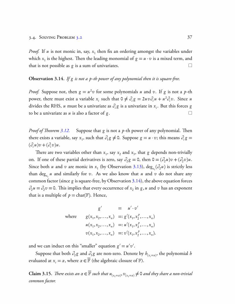
.. S P . 37

Proof. If u is not monic in, say, x1 then fix an ordering amongst the variables underwhich x1 is the highest. en the leading monomial of g = u · v is a mixed term, andthat is not possible as g is a sum of univariates.

Observation 3.14. If g is not a p-th power of any polynomial then it is square-free.

Proof. Suppose not, then g = u2v for some polynomials u and v. If g is not a p-thpower, there must exist a variable xi such that 0 6= ∂i g = 2uv∂i u + u2∂i v. Since u

divides the RHS, u must be a univariate as ∂i g is a univariate in xi . But this forces g

to be a univariate as u is also a factor of g .

Proof of eorem 3.12. Suppose that g is not a p-th power of any polynomial. enthere exists a variable, say x1, such that ∂1 g 6= 0. Suppose g = u · v; this means ∂i g =(∂i u)v +(∂i v)u.

ere are two variables other than x1, say x2 and x3, that g depends non-triviallyon. If one of these partial derivatives is zero, say ∂2 g = 0, then 0 = (∂2u)v + (∂2v)u.Since both u and v are monic in x1 (by Observation 3.13), degx1

(∂2u) is strictly lessthan degx1

u and similarly for v. As we also know that u and v do not share anycommon factor (since g is square-free, by Observation 3.14), the above equation forces∂2u = ∂2v = 0. is implies that every occurrence of x2 in g , u and v has an exponentthat is a multiple of p = char(F). Hence,

g ′ = u ′ · v ′where g (x1, x2, . . . , xn) =: g ′(x1, x p

2 , . . . , xn)

u(x1, x2, . . . , xn) =: u ′(x1, x p2 , . . . , xn)

v(x1, x2, . . . , xn) =: v ′(x1, x p2 , . . . , xn).

and we can induct on this “smaller” equation g ′ = u ′v ′.Suppose that both ∂2 g and ∂3 g are non-zero. Denote by h(xi=α)

, the polynomial h

evaluated at xi = α, where α ∈ F (the algebraic closure of F).

Claim 3.15. ere exists an α ∈ F such that u(x1=α), v(x1=α)

6= 0 and they share a non-trivialcommon factor.

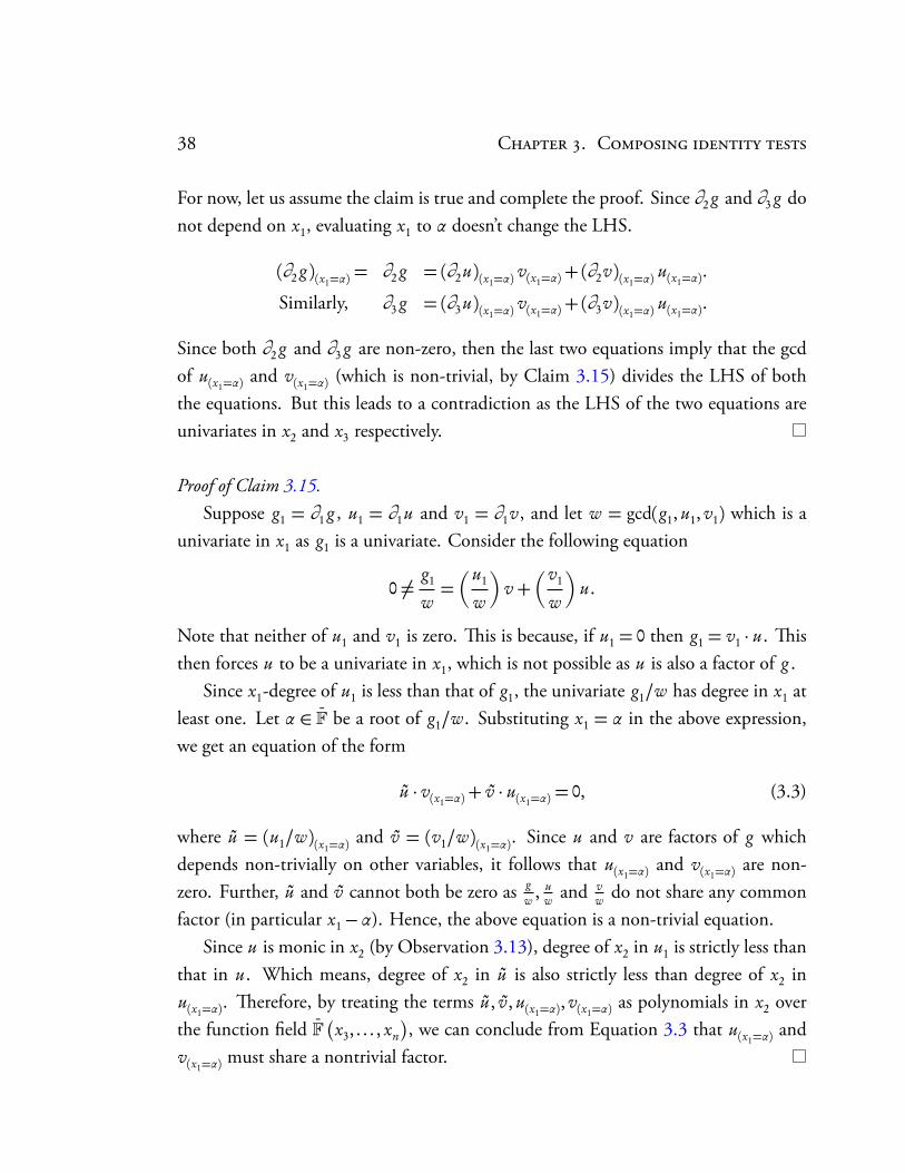
38 C . C

For now, let us assume the claim is true and complete the proof. Since ∂2 g and ∂3 g donot depend on x1, evaluating x1 to α doesn’t change the LHS.

(∂2 g )(x1=α)= ∂2 g = (∂2u)(x1=α)

v(x1=α)+(∂2v)(x1=α)

u(x1=α).

Similarly, ∂3 g = (∂3u)(x1=α)v(x1=α)

+(∂3v)(x1=α)u(x1=α)

.

Since both ∂2 g and ∂3 g are non-zero, then the last two equations imply that the gcdof u(x1=α)

and v(x1=α)(which is non-trivial, by Claim 3.15) divides the LHS of both

the equations. But this leads to a contradiction as the LHS of the two equations areunivariates in x2 and x3 respectively.

Proof of Claim 3.15.Suppose g1 = ∂1 g , u1 = ∂1u and v1 = ∂1v, and let w = gcd(g1, u1, v1) which is a

univariate in x1 as g1 is a univariate. Consider the following equation

0 6= g1

w=u1

w

v +

v1

w

u.

Note that neither of u1 and v1 is zero. is is because, if u1 = 0 then g1 = v1 · u. isthen forces u to be a univariate in x1, which is not possible as u is also a factor of g .

Since x1-degree of u1 is less than that of g1, the univariate g1/w has degree in x1 atleast one. Let α ∈ F be a root of g1/w. Substituting x1 = α in the above expression,we get an equation of the form

u · v(x1=α)+ v · u(x1=α)

= 0, (3.3)

where u = (u1/w)(x1=α)and v = (v1/w)(x1=α)

. Since u and v are factors of g whichdepends non-trivially on other variables, it follows that u(x1=α)

and v(x1=α)are non-

zero. Further, u and v cannot both be zero as gw , u

w and vw do not share any common

factor (in particular x1−α). Hence, the above equation is a non-trivial equation.Since u is monic in x2 (by Observation 3.13), degree of x2 in u1 is strictly less than

that in u. Which means, degree of x2 in u is also strictly less than degree of x2 inu(x1=α)

. erefore, by treating the terms u, v, u(x1=α), v(x1=α)

as polynomials in x2 overthe function field Fx3, . . . , xn

, we can conclude from Equation 3.3 that u(x1=α)

andv(x1=α)

must share a nontrivial factor.

.. S P . 39

3.4.3 Finishing the argument

eorem 3.11 and 3.12 essentially give the solution to Problem 3.2. Although, e-orem 3.12 justifies our assumption of gi ’s being essentially coprime when gi dependson three or more variables, we need to slightly change our strategy for gi ’s that arebivariates or univariates. In this case, we first take pairwise gcd of the bivariates (sim-ilarly, pairwise gcd of the univariates) and factorize accordingly till all the bivariates(similarly, the univariates) are mutually coprime. Taking gcd of two bivariate (monic)polynomials takes only polynomial time using Euclidean gcd algorithm (by long divi-sion). Once coprimeness is ensured, we can directly check if a bivariate g di

i divides f

by expressing f as f =∑

j f j m j , where f j ’s are bivariate polynomials depending on thesame two variables as gi , and m j ’s are monomials in the remaining variables. en,

g dii | f if and only if g di

i | f j for all j .

Once again, just like gcd, bivariate divisibility is a polynomial time computation (sim-ply by long division). Finally, we can use chinese remaindering to complete the argu-ment in a similar fashion as in Section 3.4.1. We now summarize this as a theorem.

eorem 3.16. Let f , g1, . . . , gt be n-variate polynomials given explicitly as a sum of at mosts monomials, each of whose degrees are bounded by d and each gi being a sum of univariates.en, we can check if f = g1 . . . gt in deterministic time poly(n, d , t , s).

40 C . C

4Identity testing via algebraic independence

4.1 Introduction

During the past decade, the quest for derandomization of PIT has yielded several re-sults on restricted models of circuits. But, fortunately, the search has been made morefocussed by a result [AV08, VSBR83] which states that a polynomial time blackboxderandomization of identity testing for depth-4 circuits (via a certain pseudo-randomgenerator) implies a quasi-polynomial time derandomization of PIT for poly-degree1

circuits.With depth-4 as the final frontier, the results that have been achieved so far include

polynomial time hitting-set generators for the following models:

• depth-2 (ΣΠ) circuits (or sparse polynomials) [KS01, AB99],

• depth-3 (ΣΠΣ) circuits with constant top fanin [SS11],

• depth-4 (ΣΠΣΠ) multilinear circuits with constant top fanin [SV11],

• constant-depth constant-read multilinear formulas [AvMV11],

• circuits generated by sparse polynomials with low transcendence degree [BMS11a].

To our knowledge, these are the only instances for which polynomial time hitting-set generators are known. e result on depth-3 bounded top fanin circuits is basedupon the Chinese Remaindering technique of [KS07] and the ideal-theoretic frame-work studied in [SS10b]. eir work followed after a sequence of developments inrank bound estimates [DS05, KS08, SS09, KS09b, SS10b], some using results fromincidence geometry (although, this result [SS11] in particular is not rank based). On

1Circuits computing polynomials with degree bounded by a polynomial function in the size of thecircuit.

42 C . I

the other hand, the results on constant-depth multilinear formulas [AvMV11, SV11]is obtained by building upon and extending the techniques of other earlier results[KMSV10, SV09, SV08] on ‘read-once’ models. At a high level, this involved a studyof the structure of multilinear formulas under the application of partial derivativeswith respect to a carefully chosen set of variables and invoking depth-3 rank bounds(cf. [SY10] for details). More recently, a third technique has emerged in [BMS11a]which is based upon the concept of algebraic independence of polynomials. ey showedthat for any given circuit C of polynomial degree and sparse polynomials f1, . . . , fm

with constant transcendence degree, a hitting-set generator for C ( f1, . . . , fm) can be con-structed in polynomial time.

4.1.1 Contribution of this chapter

With these diverse techniques floating around the study of hitting-set generators, onewonders: Could there be one single tool that is sufficiently powerful to capture allthese models? Is there any unique feature underlying these seemingly different modelsthat can lend itself to the conception of such a unifying tool? e answer to boththese questions, as we shall see in this chapter, is yes. e key to this lies in studyingthe properties of the Jacobian, a mathematical object lying at the very core of algebraicindependence. And as for the ‘unique feature’, notice that in the above four modelssome parameter of the circuit is bounded – be it bounded top fanin, bounded read ofvariables, or bounded transcendence degree. At an intuitive level, it seems to us that itis this ‘bounded parameter’-ness of the circuit that makes the Jacobian perform at itsbest.

In the process of finding a universal technique, we strengthen the earlier resultssignificantly thus giving the first blackbox PIT for these generalized models. BesidesΣΠΣ(k) circuits, we construct blackbox PITs for circuits of the form C (T1, · · · ,Tm)where C is any polynomial of polynomial degree and Ti ’s are products of linear func-tions with bounded transcendence degree. Further, we remove the multilinear restric-tion completely from the constant-depth constant-read models. e notion of ‘read’is also replaced by a general notion of ‘occur’ , which additionally generalizes PIT onmultilinear ΣΠΣΠ(k) circuits as well.

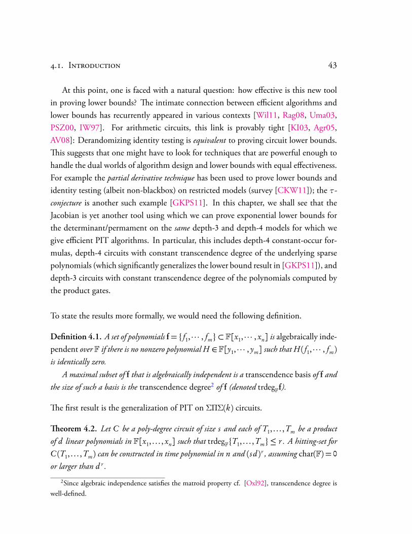
.. I 43

At this point, one is faced with a natural question: how effective is this new toolin proving lower bounds? e intimate connection between efficient algorithms andlower bounds has recurrently appeared in various contexts [Wil11, Rag08, Uma03,PSZ00, IW97]. For arithmetic circuits, this link is provably tight [KI03, Agr05,AV08]: Derandomizing identity testing is equivalent to proving circuit lower bounds.is suggests that one might have to look for techniques that are powerful enough tohandle the dual worlds of algorithm design and lower bounds with equal effectiveness.For example the partial derivative technique has been used to prove lower bounds andidentity testing (albeit non-blackbox) on restricted models (survey [CKW11]); the τ-conjecture is another such example [GKPS11]. In this chapter, we shall see that theJacobian is yet another tool using which we can prove exponential lower bounds forthe determinant/permament on the same depth-3 and depth-4 models for which wegive efficient PIT algorithms. In particular, this includes depth-4 constant-occur for-mulas, depth-4 circuits with constant transcendence degree of the underlying sparsepolynomials (which significantly generalizes the lower bound result in [GKPS11]), anddepth-3 circuits with constant transcendence degree of the polynomials computed bythe product gates.

To state the results more formally, we would need the following definition.

Definition 4.1. A set of polynomials f= f1, · · · , fm ⊂ F[x1, · · · , xn] is algebraically inde-pendent over F if there is no nonzero polynomial H ∈ F[y1, · · · , ym] such that H ( f1, · · · , fm)is identically zero.

A maximal subset of f that is algebraically independent is a transcendence basis of f andthe size of such a basis is the transcendence degree2 of f (denoted trdegFf).

e first result is the generalization of PIT on ΣΠΣ(k) circuits.

eorem 4.2. Let C be a poly-degree circuit of size s and each of T1, . . . ,Tm be a productof d linear polynomials in F[x1, . . . , xn] such that trdegFT1, . . . ,Tm ≤ r . A hitting-set forC (T1, . . . ,Tm) can be constructed in time polynomial in n and (s d )r , assuming char(F) = 0

or larger than d r .

2Since algebraic independence satisfies the matroid property cf. [Oxl92], transcendence degree iswell-defined.

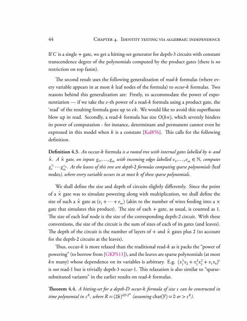
44 C . I

If C is a single + gate, we get a hitting-set generator for depth-3 circuits with constanttranscendence degree of the polynomials computed by the product gates (there is norestriction on top fanin).

e second result uses the following generalization of read-k formulas (where ev-ery variable appears in at most k leaf nodes of the formula) to occur-k formulas. Tworeasons behind this generalization are: Firstly, to accommodate the power of expo-nentiation — if we take the e-th power of a read-k formula using a product gate, the‘read’ of the resulting formula goes up to ek. We would like to avoid this superfluousblow up in read. Secondly, a read-k formula has size O(kn), which severely hindersits power of computation - for instance, determinant and permanent cannot even beexpressed in this model when k is a constant [Kal85b]. is calls for the followingdefinition.

Definition 4.3. An occur-k formula is a rooted tree with internal gates labelled by + and×. A × gate, on inputs g1, . . . , gm with incoming edges labelled e1, . . . , em ∈ N, computesg e1

1 · · · g emm . At the leaves of this tree are depth-2 formulas computing sparse polynomials (leaf

nodes), where every variable occurs in at most k of these sparse polynomials.

We shall define the size and depth of circuits slightly differently. Since the pointof a × gate was to simulate powering along with multiplication, we shall define thesize of such a × gate as (e1+ · · ·+ em) (akin to the number of wires feeding into a ×gate that simulates this product). e size of each + gate, as usual, is counted as 1.e size of each leaf node is the size of the corresponding depth-2 circuit. With theseconventions, the size of the circuit is the sum of sizes of each of its gates (and leaves).e depth of the circuit is the number of layers of + and × gates plus 2 (to accountfor the depth-2 circuits at the leaves).

us, occur-k is more relaxed than the traditional read-k as it packs the “power ofpowering” (to borrow from [GKPS11]), and the leaves are sparse polynomials (at mostkn many) whose dependence on its variables is arbitrary. E.g. (x3

1 x2 + x21 x2

3 + x1x4)e

is not read-1 but is trivially depth-3 occur-1. is relaxation is also similar to “sparse-substituted variants” in the earlier results on read-k formulas.

eorem 4.4. A hitting-set for a depth-D occur-k formula of size s can be constructed intime polynomial in s R, where R= (2k)4D ·2D (assuming char(F) = 0 or > s R).

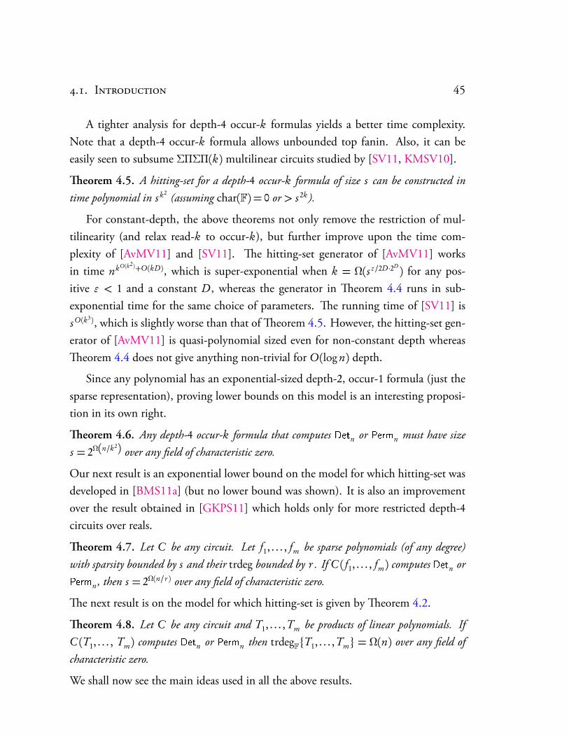
.. I 45

A tighter analysis for depth-4 occur-k formulas yields a better time complexity.Note that a depth-4 occur-k formula allows unbounded top fanin. Also, it can beeasily seen to subsume ΣΠΣΠ(k) multilinear circuits studied by [SV11, KMSV10].

eorem 4.5. A hitting-set for a depth-4 occur-k formula of size s can be constructed intime polynomial in s k2 (assuming char(F) = 0 or > s 2k).

For constant-depth, the above theorems not only remove the restriction of mul-tilinearity (and relax read-k to occur-k), but further improve upon the time com-plexity of [AvMV11] and [SV11]. e hitting-set generator of [AvMV11] worksin time nkO(k2)+O(kD), which is super-exponential when k = Ω(sε/2D ·2D ) for any pos-itive ε < 1 and a constant D, whereas the generator in eorem 4.4 runs in sub-exponential time for the same choice of parameters. e running time of [SV11] issO(k3), which is slightly worse than that of eorem 4.5. However, the hitting-set gen-erator of [AvMV11] is quasi-polynomial sized even for non-constant depth whereaseorem 4.4 does not give anything non-trivial for O(log n) depth.

Since any polynomial has an exponential-sized depth-2, occur-1 formula (just thesparse representation), proving lower bounds on this model is an interesting proposi-tion in its own right.

eorem 4.6. Any depth-4 occur-k formula that computes Detn or Permn must have sizes = 2Ω(n/k

2) over any field of characteristic zero.

Our next result is an exponential lower bound on the model for which hitting-set wasdeveloped in [BMS11a] (but no lower bound was shown). It is also an improvementover the result obtained in [GKPS11] which holds only for more restricted depth-4circuits over reals.

eorem 4.7. Let C be any circuit. Let f1, . . . , fm be sparse polynomials (of any degree)with sparsity bounded by s and their trdeg bounded by r . If C ( f1, . . . , fm) computes Detn orPermn, then s = 2Ω(n/r ) over any field of characteristic zero.

e next result is on the model for which hitting-set is given by eorem 4.2.

eorem 4.8. Let C be any circuit and T1, . . . ,Tm be products of linear polynomials. IfC (T1, . . . , Tm) computes Detn or Permn then trdegFT1, . . . ,Tm = Ω(n) over any field ofcharacteristic zero.

We shall now see the main ideas used in all the above results.

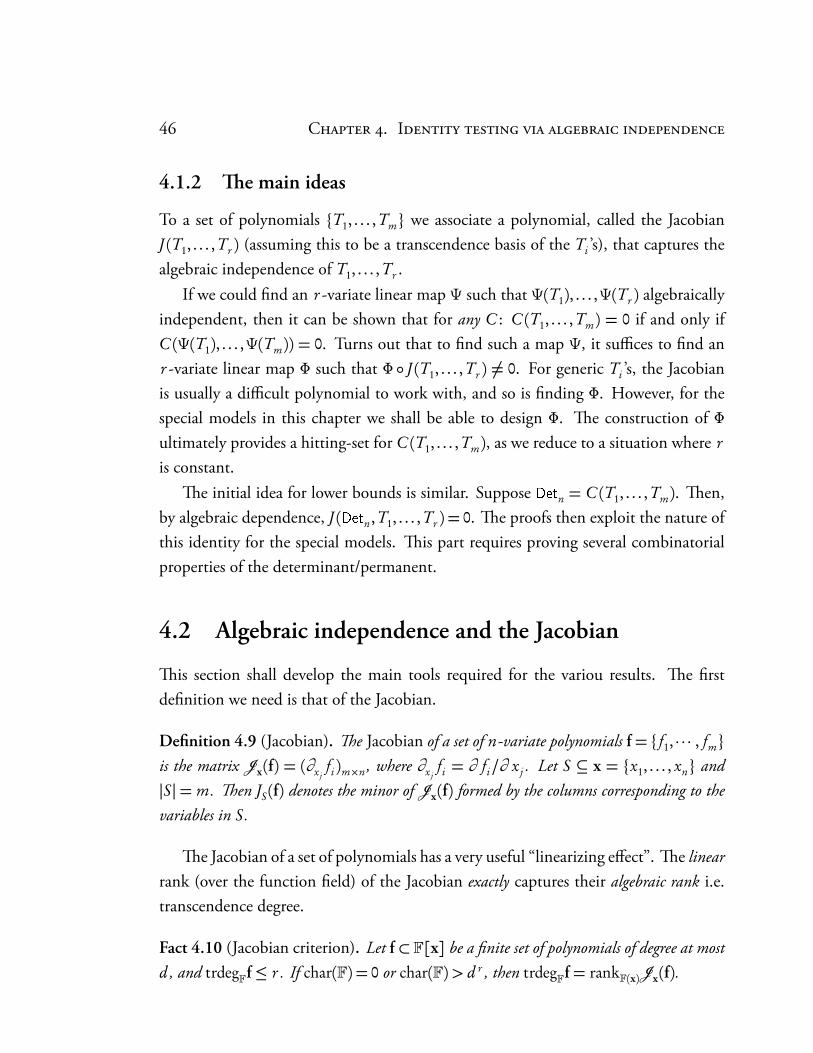
46 C . I

4.1.2 e main ideas

To a set of polynomials T1, . . . ,Tm we associate a polynomial, called the JacobianJ (T1, . . . ,Tr ) (assuming this to be a transcendence basis of the Ti ’s), that captures thealgebraic independence of T1, . . . ,Tr .

If we could find an r -variate linear map Ψ such that Ψ(T1), . . . ,Ψ(Tr ) algebraicallyindependent, then it can be shown that for any C : C (T1, . . . ,Tm) = 0 if and only ifC (Ψ(T1), . . . ,Ψ(Tm)) = 0. Turns out that to find such a map Ψ, it suffices to find anr -variate linear map Φ such that Φ J (T1, . . . ,Tr ) 6= 0. For generic Ti ’s, the Jacobianis usually a difficult polynomial to work with, and so is finding Φ. However, for thespecial models in this chapter we shall be able to design Φ. e construction of Φultimately provides a hitting-set for C (T1, . . . ,Tm), as we reduce to a situation where r

is constant.e initial idea for lower bounds is similar. Suppose Detn = C (T1, . . . ,Tm). en,

by algebraic dependence, J (Detn,T1, . . . ,Tr ) = 0. e proofs then exploit the nature ofthis identity for the special models. is part requires proving several combinatorialproperties of the determinant/permanent.

4.2 Algebraic independence and the Jacobian

is section shall develop the main tools required for the variou results. e firstdefinition we need is that of the Jacobian.

Definition 4.9 (Jacobian). e Jacobian of a set of n-variate polynomials f= f1, · · · , fmis the matrix Jx(f) = (∂x j

fi )m×n, where ∂x jfi = ∂ fi/∂ x j . Let S ⊆ x = x1, . . . , xn and

|S | = m. en JS(f) denotes the minor of Jx(f) formed by the columns corresponding to thevariables in S.

e Jacobian of a set of polynomials has a very useful “linearizing effect”. e linearrank (over the function field) of the Jacobian exactly captures their algebraic rank i.e.transcendence degree.

Fact 4.10 (Jacobian criterion). Let f⊂ F[x] be a finite set of polynomials of degree at mostd , and trdegFf≤ r . If char(F) = 0 or char(F)> d r , then trdegFf= rankF(x)Jx(f).

.. A J 47

e proof of this fact may be seen in [BMS11b].

e next definition we need is that of a faithful homomorphism.

Definition 4.11 (Faithful homomorphism). A homomorphism Φ : F[x] → F[y] (y isanother set of variables) is said to be faithful to a finite set of polynomials f1, . . . , fm ⊂ F[x]if

trdegF f1, . . . , fm= trdegF Φ( f1), . . . ,Φ( fm) .e intuition is that trdegF fmeasures the number of “effective variables” present

amongst them. All the PITs in this chapter would try to construct a faithful homo-morphism to F[y1, . . . , yr ] where r ≈ trdegF f.

e following result asserts that faithful homomorphisms for f do not change non-zeroness any polynomial combination of f.

eorem 4.12 (Faithful preserves nonzeroness). Let f = f1, · · · , fm ⊂ F[x] and Φbe a homomorphism faithful to f. For any polynomial C ∈ F[y1, · · · , ym], C (f) = 0⇔C (Φ(f)) = 0.

Before we see the proof, it would be useful to illustrate why this result is surprising.Let us say f1, . . . , fr is one maximal algebraically independent and Φ is a map thatensures that Φ( f1), . . . ,Φ( fr ) continue to remain algebraically independent. However,the circuit C could involve only fs+1, . . . , fm and it is far from obvious why just thissuffices to preserve relations between them. But the fact that f1, . . . , fs is a maximalalgebraically independent set forces all relations amongst the fi ’s to be preserved exactlyby Φ.

e first proof of was by Beecken, Mittmann and Saxena [BMS11b] and used adeep theorem from algebraic geometry called Krull’s hauptidealsatz. e following isan alternate elementary proof of the above theorem using only basic field theory.

Proof of eorem 4.12. Since Φ is faithful to f, there is a transcendence basis (say,f1, . . . , fs ) of f such that Φ( f1), . . . ,Φ( fs ) is a transcendence basis of Φ(f). e functionfield K= F(f) essentially consists of elements that are polynomials in fs+1, . . . , fm withcoefficients from F( f1, . . . , fs ). Treating C (f) as a nonzero element of K, there is aninverse Q ∈K such that Q ·C = 1. Since Q is a polynomial in fs+1, . . . , fm with coeffi-cients from F( f1, . . . , fs ), by clearing off the denominators of these coefficients in Q, we

48 C . I

get an equation Q ·C = P ( f1, . . . , fs ), where Q is a nonzero polynomial in f and P is anonzero polynomial in f1, . . . , fs . ApplyingΦ to both sides of the equation, we concludethat C (Φ(f)) = Φ(C (f)) 6= 0, otherwise P (Φ( f1), . . . ,Φ( fs )) = Φ(P ( f1, . . . , fs )) = 0 whichis not possible as Φ( f1), . . . ,Φ( fs ) are algebraically independent and P is a nontrivialpolynomial.

A recipe for constructing faithful maps

Given a set of polynomials f1, . . . , fm, the goal is to construct a map Φ such thatΦ( f1), . . . ,Φ( fm) continue to stay algebraically independent. By the Jacobian Crite-rion (Fact 4.13), we want to ensure that the rank of J (Φ( f1), . . . ,Φ( fm)) is equal to therank of J ( f1, . . . , fm). e first step forward would be to understand how the Jacobianevolves under such a homomorphism.

Fact 4.13 (Chain rule). For any finite set of polynomials f1, . . . , fm ⊂ F[x] and a homo-morphism Φ : F[x]→ F[y], we have

Jy(Φ( f1), . . . ,Φ( fm)) = ΦJx( f1, . . . , fm)

· Jy(Φ(x1), . . . ,Φ(xn)) (4.1)

e proof of this fact follows directly from the chain-rule for differentiation.

e matrix Φ(Jx( f1, . . . , fm)) is an m×n matrix, andJy(Φ(x1), . . . ,Φ(xn)) is an n× r

matrix. Suppose we ensure that Φ(Jx(f)) has the same rank as Jx(f), we additionallyneed to ensure that post-multiplication byJy(Φ(x)) does not change the rank. Similarquestions have been studied earlier in the context of rank extractors by Gabizon andRaz [GR05], and it is known that post-multiplication by a (suitable) Vandermondematrix preserves the rank.

Lemma 4.14 ([GR05]). Let A be a m×n matrix with entries in a field F, and let t be anindeterminate. en, rankF(t )

A · (t i j )i∈[n], j∈[m]

= rankFA.

e next theorem shall simulate this by augmenting the map Φ slightly to makethe matrix on the right of Equation (4.1) a Vandermonde matrix (essentially).

Lemma 4.15 (Composition Lemma). Let f⊂ F[x] be a finite set of polynomials of degreeat most d , trdegFf≤ r , and char(F) = 0 or> d r . Let Φ : F[x]→ F[z] be a homomorphism

.. D-3 49

such that rankF(x)Jx(f) = rankF(z)Φ(Jx(f)). en, the map Ψ : F[x]→ F[z, t , y1, . . . , yr ]such that

Ψ(xi ) 7→ r∑

j=1

y j ti j

+Φ(xi ) for 1≤ i ≤ n

is a homomorphism faithful to f.

Proof. Without loss of generality, let trdegF(f) = r , which (by Jacobian criterion) is therank of Jx(f). We intend to show that the matrix Jy(Ψ(f)) is of rank r , which wouldimply (by Jacobian criterion) that trdegF(t ,z) Ψ(f) = r . Consider the projection J ′ ofJy(Ψ(f)) obtained by setting y1 = · · ·= yr = 0.

J ′ = Jy(Ψ(f))

y=0=

Ψ(Jx(f)) · Jy(Ψ(x))

y=0

(By chain rule)

= Φ(Jx(f)) · Jy(Ψ(x))

Observe that the matrix Jy(Ψ(x)) is exactly the Vandermonde matrix that is presentin Lemma 4.14. Also, Φ(Jx(f)) has entries in F(z), and by assumption has the samerank as Jx(f). Hence, by Lemma 4.14,

rankF(t ,z)J ′ = rankF(t ,z)

Φ(Jx(f)) · Jy(Ψ(x))

= rankF(z)Φ(Jx(f)) = r.

And since J ′ is just a projection of Jy(Ψ(f)), the rank of the latter must also be r .Hence, Ψ is indeed faithful.

e different results in this chapter would be constructions of such a map Φ thatpreserves the rank of the Jacobian, which by the above lemma can be augments to givea faithful map.

4.3 Depth-3 circuits of bounded transcendence degree

Let C be any circuit of polynomial degree and D = C (T1, · · · ,Tm), where each Ti isof the form

∏dj=1 `i j , every `i j is a linear polynomial in F[x1, . . . , xn]. Denote by T

the set T1, . . . ,Tm and by L(Ti ) the multiset of linear polynomials that constitute Ti .is section shall present a hitting set for such circuits where trdegF T is boundedby a constant. Note that ΣΠΣ(k) circuit is a special case of such a circuit where thecircuit D =C (T1, . . . ,Tk) where C is a + gate.

50 C . I

Suppose trdegF T = k ≤ r and Tk = T1, . . . ,Tk be a transcendence basis ofT. Since Jx(Tk) has full rank (char(F) = 0 or char(F) > d r ), without loss of gen-erality assume that the columns corresponding to xk = x1, · · · , xk form a nonzerok × k minor of Jx(Tk). By Lemma 4.15, if we construct a Φ : F[x] → F[z] thatkeeps Jxk

(Tk) nonzero then Φ can easily be extended to a homomorphism Ψ : F[x]→F[z, t , y1, . . . , yr ] that is faithful to T. And hence, by eorem 4.12, it would followthat Ψ(D) = 0 if and only if D = 0.

4.3.1 Preserving non-zeroness of Jxk(Tk)

Let us first understand the structure of Jxk(Tk). If Ti =

∏dj=1 `i j then

∂xTi = Ti · d∑

j=1

∂x`i j

`i j

By expanding, using this additive structure of ∂xTi and the linearity of determinantwith respect to rows, the determinant Jxk

(Tk) takes the following form,

Jxk(Tk) =

∑`1∈L(T1),...,`k∈L(Tk )

T1 · · ·Tk

`1 · · ·`k

· Jxk(`1, · · · ,`k). (4.2)

We shall call a set of linear polynomials independent if the correponding homoge-nous linear parts (i.e. the constant-free parts) are F-linearly independent. e termJxk(`1, · · · ,`k) ensures that the above sum is only over those `1, · · · ,`k that are in-

dependent linear polynomials (otherwise Jxk(`1, . . . ,`k) is zero). e sum in equa-

tion (4.2) has the form of a depth-3 circuit. We shall call it H0, and we intend toconstruct a low-variate Φ such that Φ(H0) 6= 0. We show that this is achieved by a Φthat preserves the independence of a ‘small’ set of linear polynomials. In other words,we would like to construct a certificate of non-zeroness of H0.Certificate of H0: We can assume that the terms Jxk

(`1, · · · ,`k) in equation (4.2) arenon-zero field constants. Let L (H0) be the set of all linear polynomials occurring inthe denominator terms “`1 · · ·`k” of all the summands in sum (4.2). By adjusting thefield constants at the numerators, we can assume that no two linear polynomials inL (H0) are constant multiple of each other. is means, the depth-3 circuit H0 has the

.. D-3 51

formH0 = T ·∑

L

αL

`1 · · ·`k

where T :=∏k

i=1 Tk , each αL is a nonzero field constant and the sum runs over setsL= `1, · · · ,`k of k independent linear polynomials in L (H0).

Let us define the content of a depth-3 circuit, G =∑

i Pi where Pi is a product oflinear polynomials, as cont(G) := gcdiPi. Also, let the simple part of G be defined assim(G) :=G/cont(G). Hence cont(H0) = gcdLT /`1 · · ·`k and

sim(H0) = F0 ·∑

L

αL

`1 · · ·`k

, where F0 =T

cont(H0), (4.3)

Note that, since ` ∈L (H0) if and only if `||F0, we see that F0 is simply the productof the linear polynomials in L (H0) and hence deg(F0) = |L (H0)|. erefore, for any` ∈ L (H0), the terms in sim(H0) that survive modulo `1 are those with `1 in thedenominator “`1 · · ·`k” of the above expression. Hence,

H1 := sim(H0)mod `1 =F0

`1

· ∑`2,··· ,`k

αL

`2 · · ·`k

We can treat H1 as a depth-3 circuit in one less variable: if `1 = c1x1+∑n

i=2 ci xi whereci ’s ∈ F and c1 6= 0, then going modulo `1 is equivalent to replacing x1 by−∑n

i=2 ci xi/c1

in sim(H0). Hence, H1 becomes a depth-3 circuit in F[x2, . . . , xn]. erefore, it makesperfect sense to talk about cont(H1) and sim(H1). Observe that `2, · · · ,`k remain in-dependent linear polynomials modulo `1, and so H1 is a depth-3 circuit of the ‘samenature’ as H0 but with one less linear polynomials in the denominators. Also, the linearpolynomials in L (H1) is a subset of the linear polynomials in L (H0) modulo `1.

Extending the above argument, we can define the following sequence of circuits:Hi := sim(Hi−1) mod ˜

i , (1≤ i ≤ k) where ˜i ∈L (Hi−1). Further, L (Hi ) is a subset

of L (Hi−1) modulo ˜i , which implies that essentially there are independent linear

polynomials, say `1, . . . ,`k , inL (H0) such that ˜i = `i mod (`1, . . . ,`i−1) and therefore

Hi = sim(Hi−1) mod (`1, . . . ,`i ).

Lemma 4.16 (Certifying path). Suppose H0 6= 0. en there exists independent linearpolynomials `1, · · · ,`k ⊆L (H0) such that Hi 6= 0 mod (`1, . . . ,`i ), ∀i ∈ [k], and Hk isa nonzero product of linear polynomials in L (H0) modulo (`1, · · · ,`k).

52 C . I

Proof. e proof is by induction on k and follows the above sketch. e degree of thenonzero polynomial sim(H0) is |L (H0)|−k. By Chinese remaindering, there exists an`1 ∈L (H0) such that H1 := sim(H0)mod `1 6= 0. In the base case (k = 1), it is easy tosee that H1 is a nonzero product of linear polynomials modulo `1. For any larger k, thedepth-3 polynomial H1 has exactly the same form as H0 but with k − 1 independentlinear polynomials in the denominators. us we can induct on this smaller valuek − 1, keeping in mind that L (Hi )⊂L (H0) modulo (`1, . . . ,`i ).

A set `1, . . . ,`k, satisfying Lemma 4.16, shall be called a certifying path of H0. Fixa certifying path `1, · · · ,`k. We shall now see that any map that preserves the linearindependence of the certifying path also preserves the non-zeroness of H0.

eorem 4.17 (Preserving the certificate). Let `1, . . . ,`k be a certifying path for H0 andΦ : F[x]→ F[z1, . . . , zk+1] be a linear map such that

∀` ∈L (H0) : rank`,`1, . . . ,`k= rankΦ(`),Φ(`1), . . . ,Φ(`k)en Φ(H0) 6= 0.

Proof. We shall denote by I j the ideal generated by the linear forms¦`1, . . . ,` j

©. e

proof would proceed by backward induction on k: Assuming Φ(Hi ) 6= 0 mod Φ(Ii ),we shall see that Φ(Hi−1) 6= 0 mod Φ(Ii−1) for k ≥ i ≥ 1.

e base case: By Lemma 4.16, Hk is a nonzero product of linear polynomials inL (H0) modulo Ik , so the definition Φ, we have that Φ(Hk) 6= 0 mod Φ(Ik).

e inductive step: By construction, Hi−1 = cont(Hi−1) · sim(Hi−1) = cont(Hi−1) ·[qi`i+Hi] mod Ii−1, for some polynomial qi . By applying Φ throughout, this impliesthat Φ(Hi−1) = Φ(cont(Hi−1)) · [Φ(qi )Φ(`i )+Φ(Hi )]mod Φ(Ii−1).

By the definition of a certifying path, Hi−1 6= 0 modIi−1 which then impliesthat cont(Hi−1) 6= 0 modIi−1. is implies that none of the linear polynomials incont(Hi−1) are present in Ii−1, and Φ continues to preserve this by definition. Hencewe infer that Φ(cont(Hi−1)) 6= 0 mod Φ(Ii−1). Also, if [Φ(qi )Φ(`i ) + Φ(Hi )] = 0 mod

Φ(Ii−1), then Φ(Hi ) = 0 mod Φ(Ii ) contradicting the induction hypothesis. Hence wehave that Φ(Hi−1) 6= 0 mod Φ(Ii−1).

Constructing Φ: Such a map Φ is almost immediate from Lemma 4.14. For any` ∈L (H0), let A` be the (k+1)×n matrix whose rows are the coefficients of the linear

.. C- - 53

forms `,`1, . . . ,`k. If Φt is defined to be the map that sends xi to∑k+1

j=1 z j ti j , the

images of `,`1, . . . ,`k under Φt can be read off from the rows of the matrix productA′`

:=A` · (t i j )i∈[n], j∈[k+1]. Lemma 4.14 asserts that the rank of A′`is equal the the rank

of A`. As A′`

is an (k + 1)× (k + 1) matrix, any non-zero minor of A′`

is a non-zeropolynomial in t of degree at most n(k+1)2 and hence has at most n(k+1)2 roots in F.us rankF(t )(A

′`) = rankF((A

′`)(t=α)) for all but n(k+1)2 many α ∈ F. By running over

all ` ∈L (H0), for all but n(k + 1)2 · |L (H0)| values of α ∈ F, we infer that Φα satisfies

rank`,`1, . . . ,`k = rankΦ(`),Φ(`1), . . . ,Φ(`k) ∀` ∈L (H0)

We shall refer to one such Φα by simply Φ. We can now finish the proof by appealingto the Lemma 4.15.

eorem 4.2 (restated). Let C be a poly-degree circuit of size s and each of T1, . . . ,Tm

be a product of d linear polynomials in F[x1, . . . , xn] such that trdegFT1, . . . ,Tm ≤ r .A hitting-set for C (T1, . . . ,Tm) can be constructed in time polynomial in n and (s d )r ,assuming char(F) = 0 or larger than d r .

Proof. As r ≥ k, we can assume that the map Φ is map from F[x] to F[z1, . . . , zr+1]as above. erefore, by Lemma 4.15, the map Ψ : F[x]→ F[y1, . . . , yr , t , z1, . . . , zr+1]defined as

Ψ : xi 7→ Φ(xi )+k∑

j=1

y j ti j

ensures that D = 0 if and only if Ψ(D) = 0. Since C is a poly-degree circuit of size s ,Ψ(C (T1, . . . ,Tm)) is a polynomial of degree n r d s O(1) in the variables y,z and t . UsingCorollary 2.2, we can construct a hitting-set for Ψ(D) in time polynomial in n(s d )r .Since construction ofΨ takes time poly(nd r ), the total time taken is poly(n, (s d )r ).

4.4 Constant-depth constant-occur formulas

is section shall focus on constant-depth constant-occur formulas. Recall that anoccur-k formula (Definition 4.3) is a tree comprising of + and × gates, with leavesconsisting of sparse plynomials such that each variable occurs in at most k of the sparsepolynomials.

54 C . I

e top fan-in of an occur-k formula could be unbounded. However, for thepurpose of identity testing, we can assume that the top fan-in is bounded as well by asimple trick.

Observation 4.18 (Top fan-in reduction). Let C be a non-constant polynomial. en,there is an i such that C :=C (x1, · · · , xi−1, xi+1, xi+1, · · · , xn)−C (x1, · · · , xn) 6= 0, assum-ing char(F)> deg(C ).

Proof. If C depends non-trivially on xi and d = degxi(C ), it is easy to see that the

coefficient of xd−1i in C is non-zero.

If C has a + gate on top then C (x) =∑m

i=1 Ti , where Ti ’s are computed by × gatesat the next level. Since xi occurs in at most k of the Ti ’s, C has top fanin at most 2k. IfC has a × gate on top then C has a + gate on top with fanin 2 and depth(C ) =D+1.erefore, C belongs to the class of depth-(D + 1) occur-2k formulas of size at most(s 2+ s ), and a + gate on top with fanin bounded by 2k. Suppose H is a hitting-setfor C , we can form a new setH ⊃H by including points (α1+1,α2, . . . ,αn), (α1,α2+1, . . . ,αn), . . . , (α1, . . . ,αn−1,αn+1) inH for every (α1,α2, . . . ,αn) ∈ H . It is easy to seethat H is a hitting-set for C and size(H ) = n · size(H ). erefore, it is sufficient ifwe construct H . By reusing symbols, assume that C is a depth-D occur-k formula ofsize s with a + gate on top having top fanin at most k.

Let C (x) =∑k

i=1 Ti . e goal is to construct aΨ that is faithful to T= T1, . . . ,Tk.Let Tr = T1, . . . ,Tr be a transcendence basis of T. Since Jx(Tr ) has full rank (ifchar(F) = 0 or > s D r ), assume that the columns corresponding to xr = x1, . . . , xr form a nonzero minor of Jx(Tr ). By Lemma 4.15, it suffices to construct a Φ thatkeeps Jxr

(Tr ) 6= 0.

Proof idea - Suppose C = T1+ · · ·+Tk where each Ti =∏

Pe j

i j . Since C is an occur-kformula, it follows that the variables x1, . . . , xr occurs in at most k r of the Pi , j ’s, sayPi ,1, . . . Pi ,k r . Hence,

∂ j Ti =

d∏

`=k r+1

P ei ,`

i ,`

!· ∂ j

k r∏`=1

P ei ,`

i ,`

!for every 1≤ i , j ≤ r

.. C- - 55

erefore, we have that

Jxr(T1, . . . ,Tr ) =

r∏

i=1

d∏`=k r+1

P ei ,`

i ,`

!Jxr(T ′1 , . . . ,T ′r )

where T ′i =k r∏=1

P ei ,`

i ,`for 1 ≤ i ≤ r . We wish to construct a map Φ to preserve the

non-zeroness of the above expression. e Jacobian term on the RHS, notice thatJxr(T ′1 , . . . ,T ′r ) is a polynomial in Pi ,` and ∂ j Pi ,`, for 1 ≤ i , j ≤ r and 1 ≤ ` ≤ k r (and

the exponents ei ,`’s are rather irrelevant besides contributing to the degree). So, if Φ isfaithful to the set P := Pi ,`,∂ j Pi ,` : 1 ≤ i , j ≤ r, 1 ≤ ` ≤ k r and the singleton setsPi ,` for 1≤ i ≤ r , k r + 1≤ `≤ d , then Φ(Jxr

(Tr )) 6= 0.Observe that the polynomials inP and the singleton sets are (zeroth and first order)

derivatives of the gates at lower levels, and further these sets involve (the derivativesof ) disjoint groups of polynomials. is disjointness ensures that the number of suchsets is at most s .

us, we have reduced the problem of constructing a faithful map Φ for T to theproblem of constructing a mapΦ′ that is faithful to at most s many sets each containingderivatives of gates at lower levels. By applying the argument recursively, we eventuallyreach the level of the sparse polynomials (the leaf nodes) where a faithful map can beconstructed using Lemma 2.3.

As an illustrative example, we shall restrict to depth-4 occur-k formulas first. egeneral case proceeds exactly along these lines.

4.4.1 Restriction to the case of depth-4

eorem 4.5 (restated). A hitting-set for a depth-4 occur-k formula of size s can beconstructed in time polynomial in s k2 (assuming char(F) = 0 or > s 2k).

Proof. Let C =∑k

i=1 Ti be a depth-4 occur-k formula, where Ti =∏d

j=1 Pei j

i j and Pi j ’sare sparse polynomials. Observation 4.18 justifies the assumption that top fanin is k.Once again, assuming Tr to be a transcendence basis of T, we need to design a Φ suchthat Φ(Jxr

(Tr )) 6= 0.Let us count the number of Pi j ’s that depend on the variables xr , the remaining

Pei j

i j ’s can be taken out common from every row of Jxr(Tr ) while computing its deter-

minant. Let ci` be the number of Pi j ’s present in Ti that depend on x`, and ci :=∑` ci`

56 C . I

is the number of Pi j ’s in Ti that depend on xr . e total number of sparse polyno-mials depending on xr is therefore

∑1≤i ,`≤r ci`. Since we have an occur-k formula,∑

i ci` ≤ k and hence∑

i ,` ci` ≤ r k ≤ k2.For an xr -dependent Pi j , we can also take P

ei j−1

i j common from the i-th row ofJxr(Tr ). e sparsity of every entry of the i-th row of the residual matrix M is bounded

by ci s ci , where s is the size of C . us, det(M ) has sparsity at most r !·∏ri=1 ci s ci = sO(k2),

which implies that Jxr(Tr ) is a product of at most s + 1 powers of sparse polynomi-

als, each of whose sparsity is bounded by sO(k2) and degree bounded by s k. Hence,by Lemma 2.3, we have our desired Φ that preserves the non-zeroness of Jxr

(Tr ).Lemma 4.15 and Corollary 2.2 gives the hitting set.

4.4.2 Generalizing to larger depth

e ideas of the depth-4 case carry over to higher depth as well. We shall need somenotation to proceed further. For any multiset of variables S, let ∆S f denote the par-tial derivative of f with respect to the variables in S (including repetitions, as S is amultiset). Let var(S) denote the set of distinct variables in S.

One of the crucial properties used in the earlier proof was that each row of theJacobian minor shared a large gcd which could be pulled out. e following lemmaformalizes that notion for larger depth.

Lemma 4.19 (Content removal). Let G be any gate in an occur-k formula and S1, · · · , Sw

be multisets of variables. en there exists another occur-k formula G′ for which, the vectorof polynomials

∆S1

G, · · · ,∆SwG=VG ·

∆S1

G′, · · · ,∆SwG′such that

1. IfG is a+ gate thenG′ is also a+ gate whose children consist of at most k ·∪w

i=1var(Si )

of the children of G, and VG = 1.

2. IfG is a × gate, thenG′ is also a × gate whose children consist of at most k ·∪w

i=1var(Si )

of the children of G, and VG =G/G′.

Further, the gates constituting G′ and VG are disjoint.

Proof. 1. Suppose G = H1 + · · ·+Hm. en at most k · | ∪ var(Si )| of its childrendepend on the variables present in ∪var(Si ); let G′ be the sum of these children.en, ∆Si

G =∆SiG′ as the other gates are independent of the variables in ∪Si .

.. C- - 57

2. Suppose G = H e11 · · ·H em

m . Since G is a gate in an occur-k formula, at mostk · |∪var(Si )| of the Hi ’s depend on the variables in ∪Si ; call these H1, · · · , Ht . LetG′ :=H e1

1 · · ·H ett and VG :=G/G′. en, ∆Si

G =VG ·∆SiG′ as claimed.

We shall say that a map is faithful to a collection of sets if it is faithful to every setin the collection. Also, we shall say that a gate is at level ` if its distance to the rootis `. Going by the ‘proof idea’, suppose at the `-th level of the recursion we want toconstruct a Ψ` that is faithful to a collection of (at most) s sets of polynomials, eachset containing at most r` partial derivatives (of order up to c`) of the gates at level `.Moreover, the sets involve derivatives of disjoint groups of gates. By Lemma 4.15, itsuffices to find a map Φ` that preserves the non-zeroness of a jacobian minor of eachof the sets of polynomials. To begin with: ` = 2 and we wish to construct a Φ2 thatpreserves the non-zeroness of a jacobian minor of just one set T := T1, . . . ,Tk, sor2 ≤ k and c2 = 0. e next lemma captures the evolution of the recursion.

Lemma 4.20 (Evolution via factoring). Let U be a set of r` derivatives (of orders up toc`) of a set of gates G` at level `, and U ′ be a transcendence basis of U . Any |U ′| × |U ′|minor of Jx(U ′) is of the form ∏

i V eii , where Vi ’s are polynomials in at most r`+1 :=

(c` + 1) · 2c`+1k · r`2 many derivatives (of order up to c`+1 := c` + 1) of disjoint groups ofchildren of G`.Proof. Let G ∈G` be a gate at level ` and U1, . . . , UtG

⊂U ′ be the set of all the deriva-tives of G present in U ′. Fix any |U ′| × |U ′| sub-matrix M of Jx(U ′). Consider thetG rows of M that contain the derivatives of U1, . . . , UtG

. ese rows together containa total of w := tG · |U ′| elements that are derivatives of G of order up to (c`+ 1). Letus view all the elements of these tG rows as a single vector

∆S1

G, · · · ,∆SwG

and ap-

ply Lemma 4.19 to express it as VG ·∆S1

G′, · · · ,∆SwG′. To bound

∪wi=1Si

, observethat each of the tG rows could potentially be derivatives of G with respect to disjointsets of c` variables, and the different columns of the Jacobian minor additionally takesderivatives of |U ′| variables. Hence,

∪wi=1var(Si )

≤ tG · c` + |U ′| ≤ tG · c` + r`. So,in det(M ) we can take VG common from each of these tG rows such that the elementspresent inside the determinant are of the form∆Si

G′, where G′ has at most k(tGc`+ r`)children.

Since |Si | ≤ c`+ 1, at most k(c`+ 1) children of G′ depend on var(Si ). If G′ is a +gate, then ∆Si

G′ is the sum of the derivatives of at most k(c`+ 1) of its children (that

58 C . I

depend on var(Si )). If G′ is a × gate computing H e11 · · ·H et

t (where t ≤ k(eGc`+ r`)),then ∆Si

G′ is a polynomial combination of the Hi ’s and¦∆T H j

©;6=T⊆Si

for each H j

depending on var(Si ). Hence in either case, ∆SiG′ is a polynomial in the children of

G′ and at most (2c`+1 − 1) · k(c` + 1) of their derivatives (of order between one and(c`+ 1)).

Summing over all the w elements ∆SiG′, the elements of the tG rows of M are

polynomials in at most k(tG c`+ r`)+w · (2c`+1−1)k(c`+1) = k(tG c`+ r`)+ tG · |U ′| ·(2c`+1−1)k(c`+1) derivatives of the children of G′. Going over all G ∈G`, det(M ) canbe expressed as a product

∏G∈G`V tG

G and a polynomial V in at most k(r`c` + r 2`) +

r 2`· (2c`+1− 1)k(c`+ 1)≤ r`+1 derivatives (of order up to c`+ 1) of a group of gates in

level `+ 1. Further, the groups of gates whose derivatives constitute the VG’s and V

are mutually disjoint (by Lemma 4.19).

To begin with, let C2 = T1, . . . ,Tk and we would like to construct a map Φ2

that preserves the non-zeroness of a non-zero Jacobian minor of the Ti ’s. ApplyingLemma 4.20 (with U = T1, . . . ,Tm), any Jacobian minor of a set U can be writtenas a product of Vi ’s that are polynomials in a set of the derivatives at lower levels. Letus denote this set of derivatives by Elem(Vi ), and define C`+1 as the collection of setsElem(Vi ) as U varies over all the sets in the collection C`. It follows from the lemmathat the groups of gates whose derivatives form the different Elem(Vi )’s are disjoint andtherefore

C`+1

≤ s . Using Lemma 4.15 & 4.20, we can lift a map Φ`+1 to constructΦ` via the following corollary.

Corollary 4.21. If Φ`+1 is faithful to C`+1 then Φ` : xi 7→∑r`

j=1 y j ,` · (t`)i j+Φ`+1(xi )

is faithful to C`, where¦

y1,`, · · · , yr`,`, t`©is a fresh set of variables.

Finally, we can obtain our hitting set by repeating the above process until C` con-sists only of sparse polynomials.

eorem 4.4 (restated). A hitting-set for a depth-D occur-k formula of size s can beconstructed in time polynomial in s R, where R = (2k)4D ·2D (assuming char(F) = 0 or> s R).

Proof. Unfolding the above recursion, we eventually reach the level of the sparse poly-nomials at depth D − 2 and are required to construct a map ΨD−2 that is faithful to

.. R 59

a collection CD−2 of at most s sets of derivatives of sparse polynomials, each set con-taining at most rD−2 elements. Using the relation between r`+1 and r` from Lemma4.20, it is easy to bound

∑r` by R= (2k)4D ·2D .

Let U ∈CD−2 with transcendence basis U ′. Any |U ′| × |U ′| minor of Jx(U ′) isa sparse polynomial with sparsity bounded by s R and degree bounded by s R. UsingCorollary 2.3, the nonzeroness of this determinant is maintained by one of the maps∆p : xi 7→ u (s R+1)i mod p as p varies from 1 to a fixed poly(s R). Since

CD−2

≤ s , one ofthe maps ∆p preserves the rank of the Jacobian of all U in CD−2 — fix such a ∆p .Lemma 4.15 implies that ΦD−2 : xi 7→∑rD−2

j=1 y j ,D−2t i jD−2 +∆p(xi ) is faithful to CD−2.

Using Corollary 4.21, we can lift this to a map Φ2 defined as

Φ2 : xi 7→D−2∑`=2

r∑j=1

y j ,`ti j`

+ ∆p(xi )

that is faithful to T1, . . . ,Tk. e map Φ2 reduces the number of variables to O(R)and hence an application of Corollary 2.2 leads to a hitting-set generator with runningtime poly(s R). For the Jacobian criterion to work we need char(F) = 0 or > s R.

4.5 Related lower bounds

As mentioned earlier, polynomial identity tests are intimately related to lower bounds.We shall now see a few lower bounds for the determinant/permanent for the modelsstudied in this chapter. e following two lemmas are at the heart of the approach toproving lower bounds. Let x := xi j : 1 ≤ i , j ≤ n and T := T1, . . . ,Tm, where Ti ’sare polynomials in F[x]. ough all the following results work for Permn as well, weshall state and prove them for the Detn for simplicity.

Lemma 4.22. Suppose Detn = C (T1, . . . ,Tm), where C is any circuit and suppose Tr =T1, . . . ,Tr be a transcendence basis of Tr with r < n. en, there exist a set of r + 1

variables xr+1 ⊂ x and an equation∑r+1

i=1 ci fi ·Mi = 0 such that Mi ’s are distinct first orderprincipal minors of M , fi ’s are distinct r × r minors of Jxr+1

(Tr ), not all fi ’s are zero, andci ∈ F∗.Lemma 4.23. If M1, · · · , Mt are distinct first order principal minors of M and

∑ti=1 fi ·Mi =

0 (not all fi ’s are zero) then the total sparsity of the fi ’s is at least 2n/2−t .

60 C . I

We shall defer the proofs of these technical lemmas to the end of the section andproceed to see how they imply the lower bounds.

4.5.1 Lower bound on depth-4 occur-k formulas

eorem 4.6 (restated). Any depth-4 occur-k formula that computes Detn must havesize s = 2Ω(n/k

2) over any field of characteristic zero.

Proof. Let C be a depth-4 occur-k formula of size s that computes Detn. Since Detn isirreducible we can assume a top + gate in C . en C :=C (x11+1, x12, . . . , xnn)−C (x)is a depth-4 occur-2k formula of size at most 2s 2 and top fanin bounded by 2k (similarargument as at the beginning of Section 4.4). Moreover, C computes the minor of M

with respect to x11 which is essentially Detn−1. By reusing symbols, assume that C is adepth-4 occur-k formula with top fanin bounded by k, and C computes Detn.

Let C =∑k

i=1 Ti = Detn, where Ti =∏d

j=1 Pei j

i j , Pi j ’s are sparse polynomials. LetTr be a transcendence basis of T= T1, . . . ,Tk. By Lemma 4.22, we have an equation∑r+1

i=1 ci fi · Mi = 0 such that fi ’s are distinct r × r minors of Jxr+1(Tr ) for some set

of r + 1 variables xr+1. Arguing in the same way as in the proof of eorem 4.5 (inSection 4.4.1), we can throw away certain common terms from the minors fi ’s and getanother equation

∑r+1i=1 gi Mi = 0, where the sparsity of each gi is s O(k2). If we apply

Lemma 4.23 on this equation, we get our desired result.

It is also natural to ask for similar lower bounds for occur-k depth-D formulas, andsuch a property can be shown under a conjecture about determinant of determinants.e conjecture is a little cumbersome to explain and omitted here. e interestedreader can see the formulation in the published version of the contents [ASSS12].

4.5.2 Lower bound on circuits generated by ΣΠ polynomials

eorem 4.7 (restated). Let C be any circuit. Let f1, . . . , fm be sparse polynomials (ofany degree) with sparsity bounded by s and their trdeg bounded by r . If C ( f1, . . . , fm)computes Detn, then s = 2Ω(n/r ) over any field of characteristic zero.

Proof. In Lemma 4.22, take the Ti ’s to be sparse polynomials with sparsity boundedby s . en, in the equation

∑r+1i=1 ci fi ·Mi = 0, each fi has sparsity sO(r ). Finally, apply

Lemma 4.23 to obtain the desired lower bound.

.. R 61

4.5.3 Lower bound on circuits generated by ΠΣ polynomials

eorem 4.8 (restated). Let C be any circuit and T1, . . . ,Tm be products of linearpolynomials. If C (T1, . . . , Tm) computes Detn then trdegFT1, . . . ,Tm=Ω(n) over anyfield of characteristic zero.

Proof of eorem 4.8. Let T = T1, · · · ,Tm be products of linear polynomials suchthat C (T1, · · · ,Tm) = Detn with Tk = T1, · · · ,Tk being a transcendence basis. ByLemma 4.22, we get

∑k+1i=1 ci fi Mi = 0 where the fi ’s are k × k minors of Jxk+1

(Tk)and wlog f1 6= 0. Like in Section 4.3, we can rewrite this equation in the formH0 := T ·∑LαL(Mk+1)/`1 · · ·`k = 0 where αL(Mk+1) :=

∑k+1i=1 αL,i Mi is an F-linear

combination of Mk+1 :=

M1, · · · , Mk+1

. Observe that H0 is a sum of products of lin-

ear polynomials, with ‘coefficients’ being F-linear combinations of Mk+1. And sincef1 6= 0, the ‘coefficient’ of M1 in H0 is a nonzero depth-3 circuit.

e idea is to apply a similar treatment as in Section 4.3 to evolve H0. e invariantthat shall be maintained is that the coefficient of M1 (modulo some linear polynomials),which is a depth-3 circuit, would stay nonzero. is would finally yield a non-triviallinear combination αL(Mk+1) = 0 mod `k whence we can apply the following lemma.

Lemma 4.24. If M1, · · · , Mt are distinct first order principal minors of M and∑t

i=1αi Mi =0 mod `k (not all αi = 0) for independent linear polynomials `k , then t + k ≥ n.

We shall refer the proof of this lemma to the end of the section as well. Formally, definethe content of a circuit H = T

∑LαL(Mk+1)/`1 · · ·`k as cont(H ) := gcdL

nT

`1···`k

o, and

define sim(H ) := H/cont(H ). Let sim(H0) have the form F0

∑LαL(Mk+1)/`1 · · ·`k .

e coefficient of M1 in the above expression is a nonzero depth-3 circuit, whose de-gree is |L (H0)| − k. erefore by Chinese remaindering, ∃`1 ∈ L (H0) such that thiscoefficient is nonzero modulo `1. Hence, we can define H1 := sim(H0)mod `1 whichhas the form H1 = F0/`1 ·∑L3`1

αL(Mk+1)/`2 · · ·`k = 0 mod `1. And like in Section 4.3,the above equation can be rewritten by replacing a variable occuring in `1 by a suit-able linear combination of the rest. us, we may write H1 = F1

∑LαL(Mk+1 mod

`1)/`2 · · ·`k = 0, and maintaining the invariant that the coefficient of M1 mod `1 isnonzero. Repeating this argument, we eventually obtain Hk := Fk ·αL(Mk+1 mod `k) =0 while the coefficient of M1 mod `k is nonzero. is implies that αL(Mk+1) = 0 mod `k

62 C . I

is a non-trivial equation. And Lemma 4.24 asserts that this is not possible unless2k + 1≥ n or k ≥ (n− 1)/2.

4.5.4 Proofs of the technial lemmas

All the following lemmas hinge on this basic fact about the determinant — if lessthan c entries of a symbolic n × n matrix is replaced by arbitrary polynomials, thedeterminant remains non-zero.

Fact 4.25. Let M = (xi j )1≤i , j≤n and M ′ be the matrix obtained by setting c < n entries ofM to arbitrary polynomials in F[x]. en we have det(M ′) 6= 0.

Proof. We shall say an entry of M ′ is corrupted if it is one of the c entries of M that hasbeen replaced by a polynomial. We shall prove this by carefully rearranging the rowsand columns so that all the corrupted entries are above the diagonal. en, since allentries below the diagonal are free, we may set all of them to zero and the determinantreduces to a single nonzero monomial.

Since less than n entries of M ′ have been altered, there exists a column that is freeof any corrupted entries. By relabelling the columns if necessary, let the first columnbe free of any corrupted entry. By relabelling the rows if necessary, we can assumethat the first row contains a corruption. is ensures that the first column is free ofany corrupted entry, and the (n − 1)× (n − 1) matrix defined by rows and columns,2 through n, contain less than c − 1 corruptions. By induction, the c − 1 corruptionsmay be moved above the diagonal by suitable row/column relabelling. And since thefirst column is untouched during the process, we now have all c corruptions above thediagonal. Now setting all entries below the diagonal to zeroes reduces the determinantto a single nonzero monomial.

Lemma 4.22 (restated). Suppose Detn =C (T1, . . . ,Tm), where C is any circuit and letTr = T1, . . . ,Tr be a transcendence basis of T with r < n. en, there exist a set ofr + 1 variables xr+1 ⊂ x and an equation

∑r+1i=1 ci fi ·Mi = 0 such that Mi ’s are distinct

first order principal minors of M , fi ’s are distinct r × r minors of Jxr+1(Tr ), not all fi ’s

are zero, and ci ∈ F∗.

.. R 63

Proof. Every column of a Jacobian Jx(·) consists of entries that are differentiated withrespect to a specific variable x; we shall say that the column is indexed by x. LetTr = T1, · · · ,Tr be a transcendence basis of T. Amongst the nonzero r × r minorsof Jx(Tr ), let us pick one (and call the matrix associated with the minor as N ) thatmaximizes the number of diagonal variables xi i : 1≤ i ≤ n indexing the columns ofN . Let S denote the set of variables indexing the columns of N .

Since r < n, there exists a diagonal variable x j j /∈ S. Consider the (r + 1)× (r + 1)minor of Jx(Detn ∪Tr ) corresponding to the columns indexed by S ′ := S ∪ ¦x j j

©-

call the associated (r+1)×(r+1)matrix N . Since, Detn =C (T), the polynomials Detn

and T1, . . . ,Tr are algebraically dependent and hence det(N ) = 0. Expanding det(N )along the first row of N , which contains signed first order minors (cofactors) of M , wehave an equation

∑r+1i=1 ci fi Mi = 0, where Mi ’s are distinct minors of M , fi ’s are distinct

r × r minors of JS ′(Tr ), and ci ∈ F∗. If Mi is the principal minor of M with respectto the variable x j j then fi = det(N ) 6= 0 (by construction).

It suffices to show that if Mi is a non-principal minor of M then fi = 0. Considerany non-principal minor Mi in the above sum, say it is the minor of M with respect toxk`. e corresponding fi is precisely the r × r minor of JS ′(Tr ) with respect to thecolumns S ′ \xk`=

S \ xk`

∪¦x j j

©. Hence, by the maximality assumption on the

number of diagonal elements of M in S, fi = 0.

Lemma 4.23 (restated). If M1, · · · , Mt are distinct first order principal minors of M

and∑t

i=1 fi ·Mi = 0 (not all fi ’s are zero) then the total sparsity of the fi ’s is at least2n/2−t .

Proof. e proof is by contradiction. e idea is to start with the equation∑t

i=1 fi Mi =0 and apply two steps — sparsity reduction and fanin reduction — alternatively, till wearrive at a contradiction in the form of an equation f j ·M j = 0, where neither f j norM j is zero if the total sparsity of the fi ’s is less than 2n/2−t .

With an equation of the form∑τ

i=1 gi Ni = 0, we associate four parameters τ, s , ηand c . ese parameters are as follows: τ is called the fanin of the equation, s is thetotal sparsity of the gi ’s (we always assume that not all the gi ’s are zero), every Ni is adistinct first order principal minor of a symbolic η× η matrix N = (xi j ), and c is themaximum number of entries of N that are set as constants. To begin with, gi = fi andNi =Mi for all 1≤ i ≤ t , so τ = t , η= n, N =M and c = 0.

64 C . I

In the ‘sparsity reduction’ step, we start with an equation∑τ

i=1 gi Ni = 0, withparameters τ, s , η, c and arrive at an equation

∑τ′i=1 g ′i N ′i = 0 with parameters τ′, s ′,

η′, c ′ such that τ′ ≤ τ, s ′ ≤ s/2, η− 1≤ η′ ≤ η, and c ′ ≤ c + 1.In the ‘fanin reduction’ step, we start with an equation

∑τi=1 gi Ni = 0, with pa-

rameters τ, s , η, c and arrive at an equation∑τ′

i=1 g ′i N ′i = 0 with parameters τ′, s ′, η′,c ′ such that one of the two cases happens — either (τ′ ≤ τ−1, s ′ ≤ s ,η′ = η−1, c ′ = c)or (τ′ = 1, s ′ ≤ s ,η′ = η, c ′ ≤ c +τ).

Naturally, starting with∑t

i=1 fi Mi = 0, the ‘sparsity reduction’ step can only beperformed at most log s many times (since the total sparsity of the gi ’s reduces by atleast a factor of half every time this step is executed), whereas the ‘fanin reduction’ stepcan be performed at most t −1 times (as the fanin goes down by at least one for everysuch step). Finally, when this process of alternating steps ends, we have an equationof the form gi ·Ni = 0, where gi 6= 0 and Ni is a principal minor of a symbolic matrixN of dimension at least n− (log s + t −1) such that at most (log s + t ) entries of N areset as constants. Now, if log s + t ≤ n − (log s + t ) the Ni can never be zero (by Fact4.25) and hence we arrive at a contradiction. erefore, s > 2n/2−t . Now, the detailsof the sparsity reduction and the fanin reduction steps.

Suppose, we have an equation∑τ

i=1 gi Ni = 0 as mentioned above. Without loss ofgenerality, assume that the minor Ni is the minor of N with respect to the i t h diagonalelement of N . Call all the variables xi j in N with both i , j > τ as the white variables.ese are the variables that are present in every minor Ni in the sum

∑τi=1 gi Ni . e

variables xi j where both i , j ≤ τ are called the black variables, and the remaining arethe grey variables. By assumption, c of the variables in N are set as constants.

Sparsity reduction step - Say x is a white variable that one of the gi ’s depends on.Writing each gi as a polynomial in x, there must be two distinct powers of x amongstthe gi ’s (for if not, then x can be taken common across all gi ’s). Let x` be the lowestdegree and x h be the highest. Dividing the entire equation

∑τi=1 gi Ni = 0 by x`,

we can further assume that ` = 0. Each of the gi ’s and Ni ’s can be expressed as,gi = gi ,0+ x · gi ,1+ · · ·+ x h · gi ,h and Ni =Ni ,0+ x ·Ni ,1, where gi , j ’s and Ni , j ’s are x-free.Looking at the coefficients of x0 and x h+1 in the equation yields

∑τi=1 gi ,0 ·Ni ,0 = 0 and∑τ

i=1 gi ,h ·Ni ,1 = 0. Note that Ni ,0’s can be thought of as principal minors of the η×ηmatrix N ′ obtained by setting x = 0 in N . And each of the Ni ,1’s can be thought of

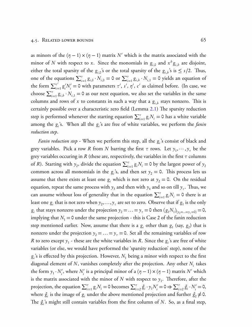
.. R 65

as minors of the (η− 1)× (η− 1) matrix N ′ which is the matrix associated with theminor of N with respect to x. Since the monomials in gi ,0 and x h gi ,h are disjoint,either the total sparsity of the gi ,0’s or the total sparsity of the gi ,h ’s is ≤ s/2. us,one of the equations

∑τi=1 gi ,0 ·Ni ,0 = 0 or

∑τi=1 gi ,h ·Ni ,1 = 0 yields an equation of

the form∑τ′

i=1 g ′i N ′i = 0 with parameters τ′, s ′, η′, c ′ as claimed before. (In case, wechoose

∑τi=1 gi ,h ·Ni ,1 = 0 as our next equation, we also set the variables in the same

columns and rows of x to constants in such a way that a gi ,h stays nonzero. is iscertainly possible over a characteristic zero field (Lemma 2.1) e sparsity reductionstep is performed whenever the starting equation

∑τi=1 gi Ni = 0 has a white variable

among the gi ’s. When all the gi ’s are free of white variables, we perform the faninreduction step.

Fanin reduction step - When we perform this step, all the gi ’s consist of black andgrey variables. Pick a row R from N barring the first τ rows. Let y1, · · · , yτ be thegrey variables occuring in R (these are, respectively, the variables in the first τ columnsof R). Starting with y2, divide the equation

∑τi=1 gi Ni = 0 by the largest power of y2

common across all monomials in the gi ’s, and then set y2 = 0. is process lets usassume that there exists at least one gi which is not zero at y2 = 0. On the residualequation, repeat the same process with y3 and then with y4 and so on till yτ. us, wecan assume without loss of generality that in the equation

∑τi=1 gi Ni = 0 there is at

least one gi that is not zero when y2, . . . , yτ are set to zero. Observe that if g1 is the onlygi that stays nonzero under the projection y2 = . . .= yτ = 0 then (g1N1)(y2=...=yτ=0) = 0,implying that N1 = 0 under the same projection - this is Case 2 of the fanin reductionstep mentioned earlier. Now, assume that there is a gi other than g1 (say, g2) that isnonzero under the projection y2 = . . .= yτ = 0. Set all the remaining variables of rowR to zero except y1 - these are the white variables in R. Since the gi ’s are free of whitevariables (or else, we would have performed the ‘sparsity reduction’ step), none of thegi ’s is effected by this projection. However, N1 being a minor with respect to the firstdiagonal element of N , vanishes completely after the projection. Any other Ni takesthe form y1 ·N ′i , where N ′i is a principal minor of a (η− 1)× (η− 1) matrix N ′ whichis the matrix associated with the minor of N with respect to y1. erefore, after theprojection, the equation

∑τi=1 gi Ni = 0 becomes

∑τi=2 gi · y1N ′i = 0⇒∑τ

i=2 gi ·N ′i = 0,where gi is the image of gi under the above mentioned projection and further g2 6= 0.e gi ’s might still contain variables from the first column of N . So, as a final step,

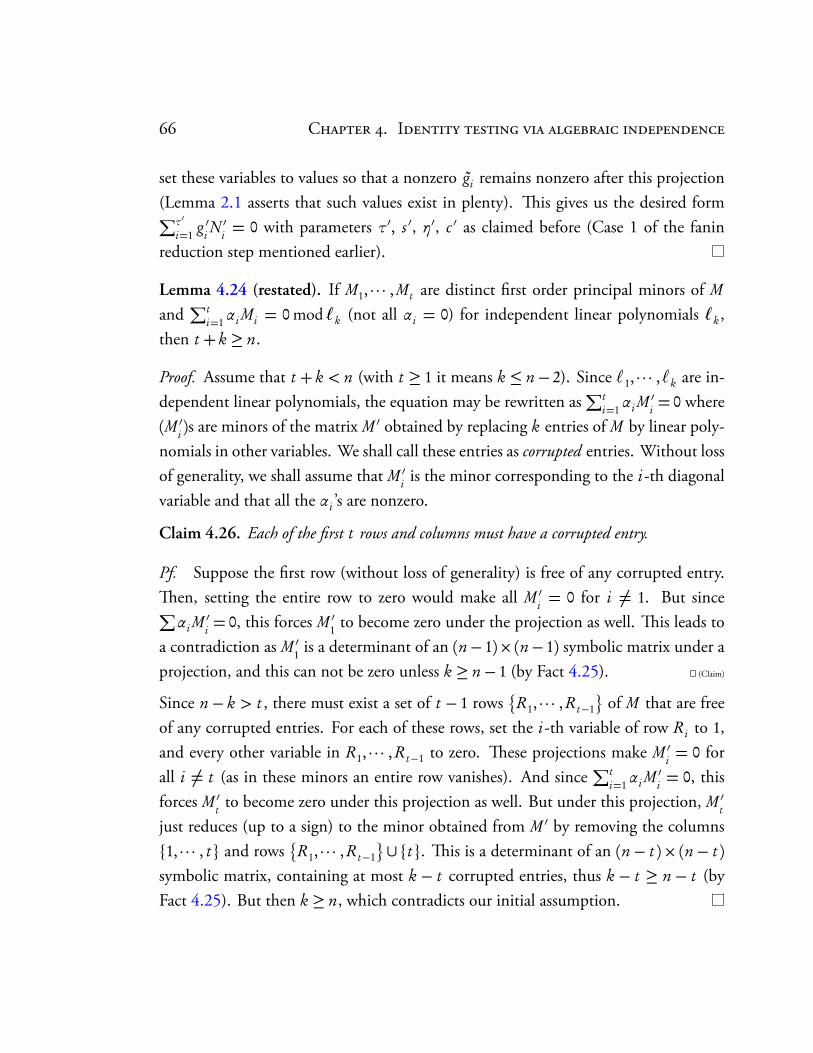
66 C . I

set these variables to values so that a nonzero gi remains nonzero after this projection(Lemma 2.1 asserts that such values exist in plenty). is gives us the desired form∑τ′

i=1 g ′i N ′i = 0 with parameters τ′, s ′, η′, c ′ as claimed before (Case 1 of the faninreduction step mentioned earlier).

Lemma 4.24 (restated). If M1, · · · , Mt are distinct first order principal minors of M

and∑t

i=1αi Mi = 0 mod `k (not all αi = 0) for independent linear polynomials `k ,then t + k ≥ n.

Proof. Assume that t + k < n (with t ≥ 1 it means k ≤ n− 2). Since `1, · · · ,`k are in-dependent linear polynomials, the equation may be rewritten as

∑ti=1αi M

′i = 0 where

(M ′i )s are minors of the matrix M ′ obtained by replacing k entries of M by linear poly-nomials in other variables. We shall call these entries as corrupted entries. Without lossof generality, we shall assume that M ′i is the minor corresponding to the i-th diagonalvariable and that all the αi ’s are nonzero.

Claim 4.26. Each of the first t rows and columns must have a corrupted entry.

Pf. Suppose the first row (without loss of generality) is free of any corrupted entry.en, setting the entire row to zero would make all M ′i = 0 for i 6= 1. But since∑αi M

′i = 0, this forces M ′1 to become zero under the projection as well. is leads to

a contradiction as M ′1 is a determinant of an (n−1)× (n−1) symbolic matrix under aprojection, and this can not be zero unless k ≥ n− 1 (by Fact 4.25). (Claim)

Since n− k > t , there must exist a set of t − 1 rows

R1, · · · , Rt−1

of M that are free

of any corrupted entries. For each of these rows, set the i-th variable of row Ri to 1,and every other variable in R1, · · · , Rt−1 to zero. ese projections make M ′i = 0 forall i 6= t (as in these minors an entire row vanishes). And since

∑ti=1αi M

′i = 0, this

forces M ′t to become zero under this projection as well. But under this projection, M ′tjust reduces (up to a sign) to the minor obtained from M ′ by removing the columns1, · · · , t and rows

R1, · · · , Rt−1

∪ t. is is a determinant of an (n− t )× (n− t )symbolic matrix, containing at most k − t corrupted entries, thus k − t ≥ n − t (byFact 4.25). But then k ≥ n, which contradicts our initial assumption.

5Approaching the chasm at depth four

5.1 Introduction

As mentioned in Chapter 1, the main motivating question in the field of arithmeticcircuit complexity is proving super-polynomial lower bounds for the permanent. epermanent, by virtue of being complete for the class VNP (an algebraic analogue ofthe class NP, defined in [Val79]), occupies a central position in the study of the com-plexity of counting problems. e best known circuit for the permanent is actually adepth three homogeneous circuit of size O(n2 ·2n) and is called the Ryser’s formula. Itsillustrious sibling, the determinant, is widely believed to be comparatively easy, beingcomplete for a subclass of VP (an algebraic analogue of P, also defined in [Val79]). Itis conjectured (cf. [AV08]) that any arithmetic circuit computing the n × n perma-nent must be of exp(n) size. Meanwhile, the arithmetic complexity of computing thedeterminant equals O(nω), whereω is the exponent of matrix multiplication. Resolv-ing the arithmetic complexity of computing the permanent and the determinant (i.e.determining the exponent of matrix multiplication) are two of the most fascinatingopen problems of our times.

5.1.1 Prior Work

Lower bounds have been obtained earlier for depth three arithmetic circuits (with somerestrictions) and constant depth multilinear circuits. Specifically, Nisan and Wigder-son [NW97] showed that any homogeneous depth three circuit computing the per-manent (also the determinant) must be of exponential size. Following that, Grigorievand Karpinski [GK98] showed that any depth three arithmetic circuit over a finite fieldcomputing the permanent (also the determinant) requires exponential size but prov-ing lower bounds for depth three circuits over fields of characteristic zero (or even overthe algebraic closure of a finite field) remains an outstanding open problem. In this

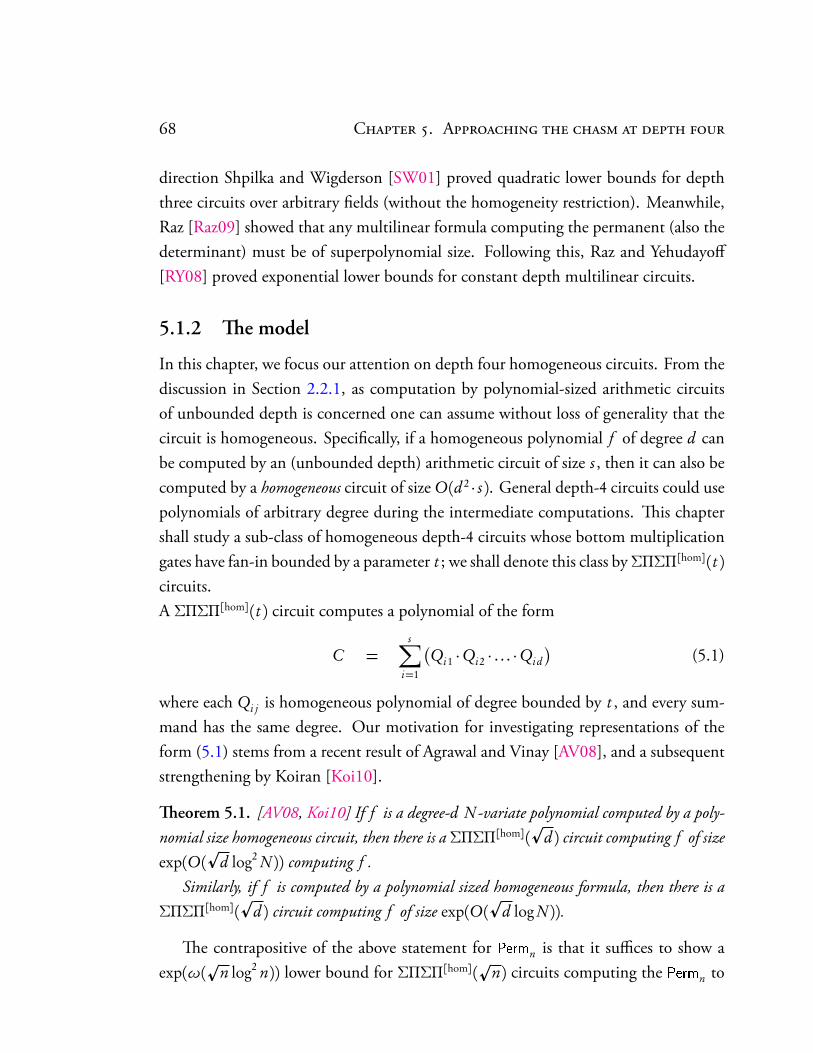
68 C . A

direction Shpilka and Wigderson [SW01] proved quadratic lower bounds for depththree circuits over arbitrary fields (without the homogeneity restriction). Meanwhile,Raz [Raz09] showed that any multilinear formula computing the permanent (also thedeterminant) must be of superpolynomial size. Following this, Raz and Yehudayoff[RY08] proved exponential lower bounds for constant depth multilinear circuits.

5.1.2 e model

In this chapter, we focus our attention on depth four homogeneous circuits. From thediscussion in Section 2.2.1, as computation by polynomial-sized arithmetic circuitsof unbounded depth is concerned one can assume without loss of generality that thecircuit is homogeneous. Specifically, if a homogeneous polynomial f of degree d canbe computed by an (unbounded depth) arithmetic circuit of size s , then it can also becomputed by a homogeneous circuit of size O(d 2 · s). General depth-4 circuits could usepolynomials of arbitrary degree during the intermediate computations. is chaptershall study a sub-class of homogeneous depth-4 circuits whose bottom multiplicationgates have fan-in bounded by a parameter t ; we shall denote this class byΣΠΣΠ[hom](t )circuits.A ΣΠΣΠ[hom](t ) circuit computes a polynomial of the form

C =s∑

i=1

Qi1 ·Qi2 · . . . ·Qi d

(5.1)

where each Qi j is homogeneous polynomial of degree bounded by t , and every sum-mand has the same degree. Our motivation for investigating representations of theform (5.1) stems from a recent result of Agrawal and Vinay [AV08], and a subsequentstrengthening by Koiran [Koi10].

eorem 5.1. [AV08, Koi10] If f is a degree-d N -variate polynomial computed by a poly-nomial size homogeneous circuit, then there is a ΣΠΣΠ[hom](

pd ) circuit computing f of size

exp(O(p

d log2 N )) computing f .Similarly, if f is computed by a polynomial sized homogeneous formula, then there is a

ΣΠΣΠ[hom](p

d ) circuit computing f of size exp(O(p

d logN )).

e contrapositive of the above statement for Permn is that it suffices to show aexp(ω(

pn log2 n)) lower bound for ΣΠΣΠ[hom](

pn) circuits computing the Permn to

.. B I O 69

prove a super-polynomial circuit lower bound. us, a good enough lower bound forΣΠΣΠ[hom](

pn) circuits would imply super-polynomial lower bounds for Permn. In

this chapter, we give a lower bound for the permanent (or determinant) that comesvery close to the above threshold.

eorem 5.2. AnyΣΠΣΠ[hom](t ) that computes the polynomial Permn (or Detn) must havesize exp

Ω

nt

.

Corollary 5.3. Any ΣΠΣΠ[hom](p

n) that computes the polyomial Permn (or Detn) musthave size exp

Ωp

n.

Remark. e results of Agrawal-Vinay [AV08] and Koiran [Koi10] depth-reduce anypolynomial sized circuit computing a degree n polynomial to a ΣΠΣΠ[hom](t ) formulawith top fanin exp

nt log2 n

. e above theorem infact is a bound on the top fanin

of ΣΠΣΠ[hom](t ) circuits computing the permanent or determinant. In Section 5.5,we shall prove a prove a generalization of eorem 5.2 by extending the lowerboundfor all circuits that are sums of arbitrary powers of O

nt

-many degree t polynomials.

Further, the proofs are completely elementary and self-contained. Also, though theabove theorem gives a lower bound for both the determinant and permanent, there isa subtle difference between the two and we discuss this in Section 5.6.

5.2 Basic Idea and Outline

e key idea is to exploit the shifted derivatives of a polynomial, which we shall nowdefine. Recall some notations (from Section 2.1): For an n-tuple i = (i1, i2, . . . , in) ∈Zn≥0, xi denotes the monomial (x i1

1 · x i22 · . . . · x in

n ) which has degree |i| def= (i1+ i2+ . . .+ in).Also, ∂ i f denotes the partial derivative of f with respect to the monomial xi,

∂ i f def=∂ i1

∂ x i11

∂ i2

∂ x i22

· · · ∂ in f

∂ x inn

!· · ·! .

For a finite subset of polynomials S ⊆ F[x], the F-span of S, denoted F-span (S), is theset of all possible F-linear combinations of polynomials in S. i.e.

F-span (S) def=

|S|∑i=1

αi · fi : αi ∈ F, fi ∈ S

.

70 C . A

With these notational preliminaries in hand, we are now ready to define the key con-cept.

Definition 5.4 (Shifted Derivatives). Let f (x) ∈ F[x] be a multivariate polynomial. espan of the `-shifted k-th order derivatives of f , denoted ⟨∂ =k f ⟩≤`, is defined as

⟨∂ =k f ⟩≤` def= F−span¦xi · (∂ j f ) : i, j ∈Zn

≥0 with |i| ≤ ` and |j|= k©

Since the set ⟨∂ =k f ⟩≤` forms an F-vector space, we shall denote by dim(⟨∂ =k f ⟩≤`) the di-mension of this space.

Recent work in arithmetic complexity has shown how ⟨∂ =k f ⟩≤` can give insightsinto the structure and complexity of f in ways that are sometimes surprising and un-expected. e dimension of partial derivatives employed by Nisan and Wigderson[NW97] in their lower bound proofs corresponds to looking at dim(⟨∂ =k f ⟩≤0). Kayal[Kay12a] showed that ⟨∂ =1 f ⟩≤1 yields a lie algebra that can help efficiently determineif f is equivalent (via an affine change of variables) to the permanent (or determi-nant). For `=∞, note that ⟨∂ =k f ⟩≤` is precisely the ideal generated by the k-th orderderivatives of f . Gupta, Kayal and Qiao [GKQ12] recently exploited the structure of⟨∂ =1 f ⟩≤∞ to devise an efficient reconstruction algorithm for random arithmetic for-mulas. Closer to the present application, Kayal [Kay12b] showed how dim(⟨∂ =k f ⟩≤`)(for suitably chosen ` and k) can be used to prove an exponential lower bound forrepresenting a polynomial as a sum of powers of bounded degree polynomials. Weshall see in this chapter that for suitably chosen values of ` and k, we can establish alarge gap between dim(⟨∂ =kPermn⟩≤`) and dim(⟨∂ =k f ⟩≤`) when f is computed by asmall ΣΠΣΠ[hom](t ) circuit. is separation shall give the lower bound.

5.2.1 Outline of the chapter

We shall execute this idea as follows. In Section 5.3 we shall give an upper boundon dim(⟨∂ =kC ⟩≤`) for C being a polynomial computed by a ΣΠΣΠ[hom](t ) circuit,i.e. when C is of the form given in equation (5.1). In Section 5.4, we shall presenta lower bound estimate for dim(⟨∂ =kPermn⟩≤`). We then combine these bounds toobtain a proof of our main theorem in Section 5.5. Finally, in Section 5.6, we discussthe possibility of improving the estimates for dim(⟨∂ =kPermn⟩≤`) obtained here.

.. S ΣΠΣΠ[hom](t ) 71

5.3 Shifted partials of ΣΠΣΠ[hom](t ) circuits

In this section we give an upper bound on dim(⟨∂ =kC ⟩≤`) when C is computed by adepth four circuit, i.e. C is of the form given in equation (5.1). We begin by notingthat dim(⟨∂ =k f ⟩≤`) is sub-additive.

Proposition 5.5. For all k ,` ≥ 0, we have dim(⟨∂ =k( f + g )⟩≤`) ≤ dim(⟨∂ =k f ⟩≤`) +dim(⟨∂ =k g ⟩≤`).Proof. By linearity of partial derivatives, we have xi · ∂ j( f + g ) = xi · ∂ j f + xi · ∂ j g .Hence,

⟨∂ =k( f + g )⟩≤` ⊆ F-span⟨∂ =k f ⟩≤` ∪ ⟨∂ =k g ⟩≤`

e proposition follows.

Let C be a depth-4 circuit computing a polynomial of the form1

C =s∑

i=1

Q ei1i1 ·Q ei2

i2 . . .Q ei d

i dwhere deg(Qi j )≤ t .

By Proposition 5.5, it suffices to understand the growth of dim(⟨∂ =kC ⟩≤`) of a singleterm (Q e1

1 . . .Q ed

d).

Proposition 5.6. If f = Q e11 . . .Q ed

dwhere each Qi ∈ F[xN ] is a polynomial of degree

bounded by t . en, for any `≥ 0,

dim(⟨∂ =k f ⟩≤`) ≤d + k − 1

k

N +(t − 1)k + `

N

Proof. Let j ∈Zd

≥0 be any d -tuple satisfying |j|= k. Using the product rule of differen-tiation,

∂ j

Q e11 . . .Q ed

d

=

∑j1+···+jd=j

∂ j1Q e1

1

. . .∂ jd Q ed

d

Let ji be the sum of the entries of the tuple ji . Note that since |j|= k we have

∑di=1 ji =

k. Hence, each term in the above sum can be written as

Q e1− j11 . . .Q ed− jd

d

· Q where∑ji = k and Q has degree at most (t k−k). us, every element of x≤`∂ =k(Q e1

1 · · ·Q ed

d)

can be written as a linear combination of

Q e1− j11 . . .Q ed− jd

d

xr where

∑ji = k and xr

1is is slightly more general than the form described in Equation (5.1).

72 C . A

is a monomial of degree at most `+(t−1)k. e total number of monomials of degreeat most `+ (t − 1)k over N variables is

N+(t−1)k+`N

, and the total number of choices

for j1+ · · ·+ jd = k isd+k−1

k

. Hence we obtain,

dim(⟨∂ =k(Q e11 · · ·Q ed

d)⟩≤`) ≤

d + k − 1

k

N +(t − 1)k + `

N

e following corollary follows directly from the above observation via sub-additivity.

Corollary 5.7. If C =∑s

i=1

∏dj=1 Q

ei j

i j where each Qi j ∈ F[xN ] is a polynomial of degreebounded by t , then for any k ≤ d

dim(⟨∂ =k(C )⟩≤`) ≤ s ·d + k − 1

k

N +(t − 1)k + `

N

Since our lower bound results are for homogeneous depth four formulae, we would

require an upper bound on d used in Corollary 5.7. Suppose the degree of the polyno-mial computed is D. It is possible that in a ΣΠΣΠ[hom](t ) circuit, several Qi j ’s couldhave degree much smaller than t and hence d could potentially be much larger thanD/t . However, by multiplying low degree Qi j ’s together and thereby ensuring thatevery Qi j (except perhaps one) have degree at least t/2, we can assume without lossof generality that d ≤ 2(D/t ) + 1. Note that this process may blow up the size of theformula, nevertheless we need this only for upper bounding dim(⟨∂ =k(C )⟩≤`), whichdoes not change since the polynomial computed by C does not change. us, we havethe following corollary,

Corollary 5.8. If C =∑s

i=1

∏dij=1 Qi j is a degree D polynomial, where each Qi j ∈ F[xN ]

is a homogeneous polynomial of degree bounded by t , then for any k ≤ 2(D/t )+ 1

dim(⟨∂ =k(C )⟩≤`) ≤ s ·2(D/t )+ k

k

N +(t − 1)k + `

N

In the next section we give a reasonable lower bound for dim(⟨∂ =k(Permn)⟩≤`) forsuitable choice of parameters k and `.

.. S P 73

5.4 Shifted partials of the Permanent

Reducing dimension computation to counting leading monomials. In this section,we shall present a lower bound for dim(⟨∂ =k(Permn)⟩≤`). Let be any admissiblemonomial ordering2. Recall that the leading monomial of a polynomial f ∈ F[x],denoted LM( f ), is the largest monomial xi under the ordering .

Proposition 5.9. Let S ⊆ F[x] be any finite set of polynomials. en

dim(F-span (S)) = #LM( f ) : f ∈ F-span (S).e proof is a simple application of Gaussian elimination. As a corollary we obtain

Corollary 5.10. For any polynomial f (x) ∈ F[x] we havedim(⟨∂ =k f ⟩≤`) ≥ #xi · LM(∂ j f ) : i, j ∈Z|x|≥0, |i| ≤ ` and |j|= k

e lower bound given by this corollary is usually a severe underestimate but fortu-nately even this will suffice for our purpose for the case when f = Permn.

Reduction to counting monomials with increasing subsequences. Let us fix tobe the lexicographic monomial ordering induced by the following ordering on thevariables: x11 · · · x1n x21 · · · xnn. Now note that any partial derivative ofPermn is just the corresponding permanental minor (or just ‘P-minor’). Hence by theabove corollary we have

dim(⟨∂ =k(Permn)⟩≤`) ≥ #

¨xi · LM(M ) :

xi is a monomial of degree at most ` andM is an (n− k)× (n− k) P-minor

«Now note that the leading monomial under of any (n − k)× (n − k) P-minor

M is just the product of the variables along the principal diagonal of M . Now if thevariables along the principal minor of M are (xi1 j1

, · · · , xin−k jn−k) then the indices satisfy

i1 < i2 < . . .< in−k and j1 < j2 < . . .< jn−k

is naturally leads to the following definition.2For more on monomial orderings and their applications in algebraic geometry, we refer the inter-

ested reader to Chapter 2 of the text by Cox, Little and O’Shea [CLO07]

74 C . A

Definition 5.11 (Increasing sequence). A sequence of variables (xi1 j1, · · · , xit jt

) is calledincreasing sequence if the indices satisfy

i1 < i2 < . . .< it and j1 < j2 < . . .< jt .

We will say that a monomial A= xj contains an increasing sequence of length t if thereexists an increasing sequence (xi1 j1

, · · · , xit jt) wherein every variable xir jr

(r ∈ [t]) divides A.

In this terminology we would then say that the leading monomial of any (n−k)×(n − k) P-minor is exactly the product of the variables in an increasing sequence oflength (n−k). Consequently for any P-minor M of size (n−k) we have that xi ·LM(M )contains an increasing sequence of length (n − k). Conversely, every monomial ofdegree at most (n − k + `) that contain an increasing sequence of length (n − k) canbe written as the leading monomial of xi ·M for some monomial xi of degree at most` and a (n− k)× (n− k) P-minor M . Hence we have:

Corollary 5.12. dim(⟨∂ =k(Permn)⟩≤`) is lower bounded by the number of distinct mono-mials of degree at most (n− k + `) over n2 variables that contain an increasing sequence oflength (n− k).

In order to count the number of monomials of degree bounded by n− k + ` thatcontain an increasing sequence, we shall restrict ourselves to a very small set of vari-ables to contribute the increasing sequence, and “fill-up” the remaining degree usingthe other variables. e “small set” that we consider here is just two diagonals – theprincipal diagonal and the one above it.

5.4.1 Restricting to two diagonals

We shall focus on the variables D2,n = xi i : 1≤ i ≤ n∪¦xi(i+1) : 1≤ i ≤ n− 1©. To

get a lower bound on monomials containing an (n − k)-length increasing sequence,we shall fix an increasing sequence Q ⊆D2,n and count all monomials m that containQ as the “leading increasing sequence” i.e. amongst all possible increasing sequencescontained in m, the predefined Q is highest under the lexicographic order definedearlier. e following lemma counts the number of increasing sequences contained inD2,n.

.. S P 75

Lemma 5.13. e number of length r increasing sequences in contained in D2,n is exactly2n−rr

.

Proof. Consider the (2n−1) variables in D2,n in the sequence x11, x12, x21, . . . , xnn. Pick-ing an increasing sequence of length r is the same as picking r of the (2n−1) variablessuch that no two adjacent variables (in the above order) are chosen. is can be thoughtas distributing the (2n− r −1) variables that won’t be picked such that there is at leastone between any two variables that are picked, and this is exactly equal to(2n− r − 1− (r − 1))+ (r + 1)− 1

(r + 1)− 1

=2n− r

r

For any variable xi j , define its companions to be the variables to its right in the samerow, or below it in the same column, i.e.

¦xi j ′ : j ′ > j

© ∪ ¦xi ′ j : i ′ > i©. Fix an

increasing sequence Q =¦

xi1 j1, . . . , xir jr

© ⊆ D2,n. Let Q ′ be the set of all companionsof variables in Q which are in D2,n. e key observation is that adding elements of Q ′

to Q does not alter the leading increasing sequence. For any increasing sequence thatuses elements of Q ′, replacing every xi ′ j ′ ∈Q ′ by the corresponding xi j ∈Q for whichit is a companion for yields a “higher” increasing sequence. Hence adding any subsetT ⊆Q ′ to Q does not alter the leading increasing sequence. Let us call the remainingvariables D2,n \ (Q ∪Q ′) as potentially forbidden variables. us, any monomial thatdoes not include any potentially forbidden variable cannot alter the leading increasingsequence.

Note that every element of D2,n besides xnn has exactly one companion in D2,n.Hence, if Q is a length r increasing sequence, the set of companions its Q ′ has cardi-nality at least (r − 1) and hence the set of forbidden variables has cardinality at most2(n− r ). Using this, the following bound follows almost immediately.

Corollary 5.14. For every n, k ,`≥ 0,

dim(⟨∂ =kPermn⟩≤`) ≥n+ k

2k

·n2+ `− 2k

n2− 2k

Proof. For any fixed length (n − k) increasing sequence Q, there are 2k potentiallyforbidden variables. us, any monomials of degree at most ` that does not include

76 C . A

the 2k potentially forbidden variables can be adjoined to Q without altering the leadingincreasing sequence. e number of monomials on n2−2k variables of degree at most` is exactly

n2+`−2kn2−2k

, and multiplying by the number of choices of Q (by Lemma 5.13)

gives the required lower bound.

5.5 Putting it all together

We shall require a few technical lemmas about the growth of binomial coefficients,factorials etc.

5.5.1 Growth of binomial estimates

Almost all bounds on the binomial coefficients follow from Stirling’s approximation.

Proposition 5.15 (Stirling’s Formula, cf. [Rom00]). ln(n!) = n ln n−n+O(ln n)

Using Stirling’s approximation for binomial coefficients eventually yield expressionsinvolving the entropy function.

Definition 5.16 (Entropy). e binary entropy function H2 is defined as

H2(x) = −x · log2(x)− (1− x) · log2(1− x)

e natural-log version of the entropy function, denoted by He is defined analogously as

He(x) = −x · ln(x)− (1− x) ln(1− x)

Lemma 5.17. For any 0< x < 1, we have x ln 1x ≤He(x)≤ x ln 1

x + x.

Lemma 5.18. For any constants α≥β> 0,

lnαn

βn

= aHe

β

α

n+O(ln n)

Proof. By Stirling’s approximation (Proposition 5.15),

ln(αn)!

(βn)!((α−β)n)! = (αn) ln(αn)−αn− (βn) ln(βn)+βn

− (α−β)n ln((α−β)n)+ (α−β)n+O(ln n)

= n(α lnα−β lnβ− (α−β) ln(α−β))+O(ln n)

= αn ·He

β

α

+O(ln n)

.. P 77

e following lemma would be useful for estimating the growth of ratio of binoimialcoefficients.

Lemma 5.19. Let a(n), f (n), g (n) : Z>0 → Z>0 be integer valued function such that( f + g ) = o(a). en,

ln(a+ f )!

(a− g )!= ( f + g ) lna ± O

( f + g )2

a

Proof.

(a+ f )!

(a− g )!= (a+ f )(a+ f − 1) . . . (a− g )

=⇒ a f +g

1− g

a

f +g ≤ (a+ f )!

(a− g )!≤ a f +g

1+

f

a

f +g

=⇒ ( f + g ) ln

1− g

a

≤ ln

(a+ f )!

(a− g )!− ( f + g ) lna ≤ ( f + g ) ln

1+

f

a

Using the fact that x

1+x ≤ ln(1+ x)≤ x for x >−1, it is easy to see that both the LHSand RHS are bounded by O

( f +g )2

a

.

5.5.2 Proof of the main theorem

We are now ready to prove the main theorem, which is a stronger form of eorem 5.2.

eorem 5.20. Let t : Z≥0 → Z≥0 be any increasing function such that t (n) = o(n).Suppose C is a circuit of the form C =

∑si=1 Q ei1

i1 · · ·Q ei d

i dwhere each Qi j is a polynomial

of degree bounded by t , and d = cn/t for some constant c . If C computes the polynomialPermn, then s ≥ exp

Ω

nt

.

Proof. From Corollary 5.7, dim(⟨∂ =kC ⟩≤`) can be upper bounded as

dim(⟨∂ =k(C )⟩≤`) ≤ s ·d + k − 1

k

n2+ `+(t − 1)k

n2

(5.2)

Also, Corollary 5.14 gives a lower bound for dim(⟨∂ =kPermn⟩≤`)

dim(⟨∂ =kPerm⟩≤`) ≥n+ k

2k

n2+ `− 2k

n2− 2k

(5.3)

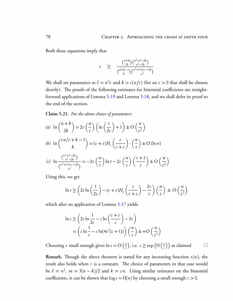
78 C . A

Both these equations imply that

s ≥n+k

2k

n2+`−2kn2−2k

d+k−1

k

n2+`+(t−1)kn2

We shall set parameters as ` = n2t and k = ε(n/t ) (for an ε > 0 that shall be chosenshortly). e proofs of the following estimates for binomial coefficients are straight-forward applications of Lemma 5.19 and Lemma 5.18, and we shall defer its proof tothe end of the section.

Claim 5.21. For the above choice of parameters:

(a) lnn+ k

2k

= 2ε

n

t

ln t

2ε

+ 1±O

n

t 2

(b) ln

cn/t + k − 1

k

= (c + ε)He

ε

c + ε

·n

t

±O (ln n)

(c) ln

n2+`−2kn2−2k

n2+`+(t−1)k

n2

=−2εn

t

ln t − 2ε

n

t

t + 1

t

±O

n

t 2

Using this, we get

ln s ≥

2ε ln 1

2ε

− (c + ε)He

ε

c + ε

− 2ε

t

n

t

± O

n

t 2

which after an application of Lemma 5.17 yields

ln s ≥

2ε ln1

2ε− ε ln

c + ε

ε

− 3ε

=ε ln

1

ε− ε ln(4e3(c + 1))

n

t

±+O

n

t 2

Choosing ε small enough gives ln s =O

nt

, i.e. s ≥ exp

Ω

nt

as claimed

Remark. ough the above theorem is stated for any increasing function t (n), theresult also holds when t is a constant. e choice of parameters in that case wouldbe ` = n2, m = 3(n − k)/2 and k = εn. Using similar estimates on the binomialcoefficients, it can be shown that log s =Ω(n) by choosing a small enough ε > 0.

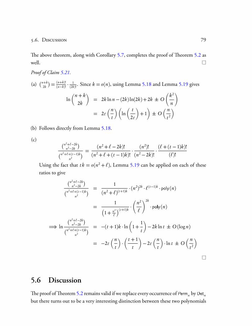
.. D 79

e above theorem, along with Corollary 5.7, completes the proof of eorem 5.2 aswell.

Proof of Claim 5.21.

(a)n+k

2k

= (n+k)!(n−k)! · 1

(2k)! . Since k = o(n), using Lemma 5.18 and Lemma 5.19 gives

lnn+ k

2k

= 2k ln n− (2k) ln(2k)+ 2k ± O

k2

n

= 2ε

n

t

ln t

2ε

+ 1± O

n

t 2

(b) Follows directly from Lemma 5.18.

(c) n2+`−2kn2−2k

n2+`+(t−1)k

n2

= (n2+ `− 2k)!

(n2+ `+(t − 1)k)!· (n2)!

(n2− 2k)!· (`+(t − 1)k)!

(`)!

Using the fact that t k = o(n2+ `), Lemma 5.19 can be applied on each of theseratios to give n2+`−2k

n2−2k

n2+`+(t−1)k

n2

= 1

(n2+ `)(t+1)k· (n2)2k · `(t−1)k · poly (n)

=1

1+ n2

`

(t+1)k·

n2

`

2k

· poly (n)

=⇒ ln

n2+`−2kn2−2k

n2+`+(t−1)k

n2

= −(t + 1)k · ln

1+1

t

− 2k ln t ± O (log n)

= −2εn

t

· t + 1

t

− 2ε

n

t

· ln t ± O

n

t 2

5.6 Discussion

e proof of eorem 5.2 remains valid if we replace every occurrence of Permn byDetn

but there turns out to be a very interesting distinction between these two polynomials

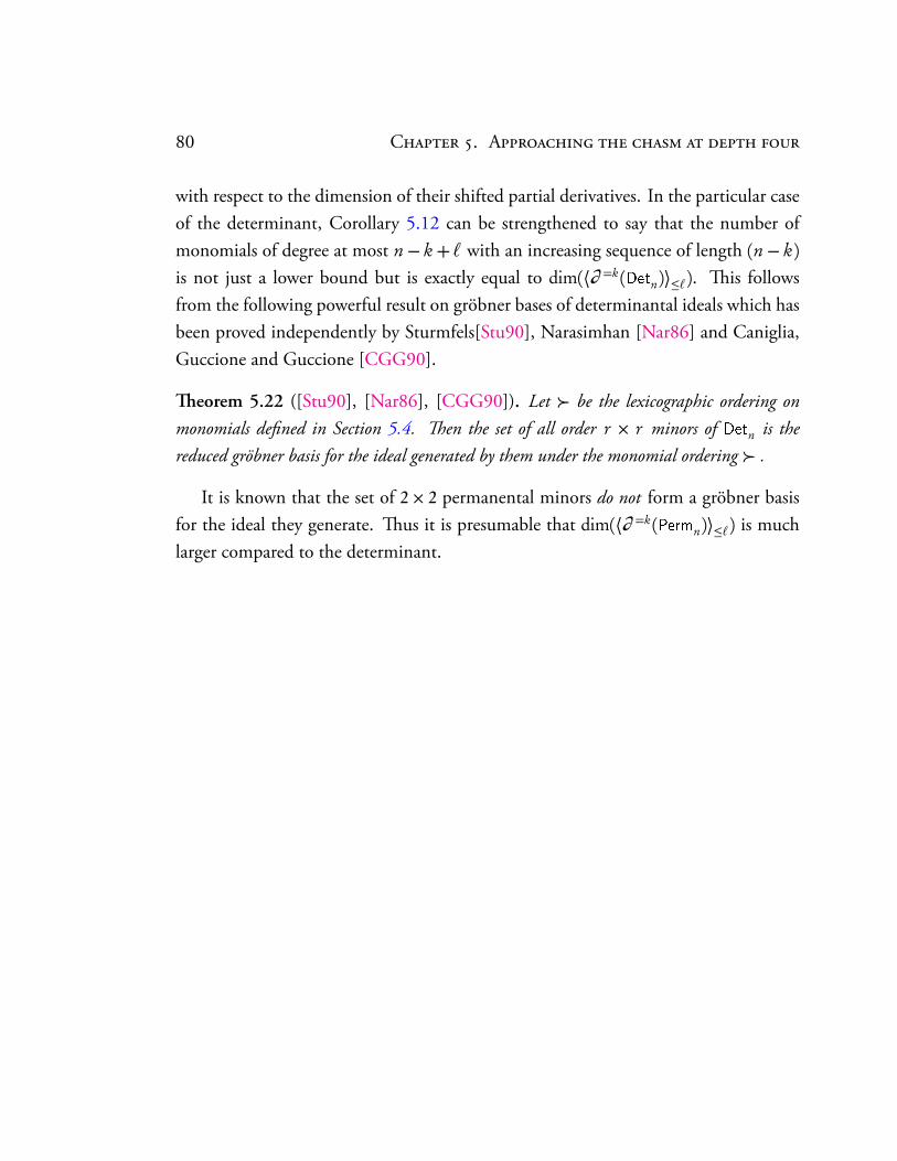
80 C . A

with respect to the dimension of their shifted partial derivatives. In the particular caseof the determinant, Corollary 5.12 can be strengthened to say that the number ofmonomials of degree at most n− k + ` with an increasing sequence of length (n− k)is not just a lower bound but is exactly equal to dim(⟨∂ =k(Detn)⟩≤`). is followsfrom the following powerful result on gröbner bases of determinantal ideals which hasbeen proved independently by Sturmfels[Stu90], Narasimhan [Nar86] and Caniglia,Guccione and Guccione [CGG90].

eorem 5.22 ([Stu90], [Nar86], [CGG90]). Let be the lexicographic ordering onmonomials defined in Section 5.4. en the set of all order r × r minors of Detn is thereduced gröbner basis for the ideal generated by them under the monomial ordering .

It is known that the set of 2× 2 permanental minors do not form a gröbner basisfor the ideal they generate. us it is presumable that dim(⟨∂ =k(Permn)⟩≤`) is muchlarger compared to the determinant.

6Conclusion and future directions

e main motivation of this thesis has been to advance our understanding of poly-nomial identity testing and lower bounds with an emphasis on a holistic approach.By providing approaches for unification, we can hopefully gain more insight into thegeneral problem of performing PIT on general circuits/formulae, or lower bounds forthe permanent.

Each of the chapters leave scope for future directions. ese are some of the obvioussteps to take towards advancing the current state-of-the-art.

6.1 Composing Identity tests

e two problems studied in Chapter 3 also have natural generalizations. e firstrelates to depth-4 fan-in 2 PIT.

Open Problem 3.1. Find a deterministic polynomial time algorithm to check if f =∏ti=1 g di

i , where f is a sparse polynomial and the gi ’s are mutually coprime, boundeddegree polynomials.

One particular case of interest is when the gi ’s are quadratic forms. Observe thata polynomial g d divides f if and only if g divides f and g d−1 divides ∂ f

∂ x1(assuming

f depends on x1 and deg( f ) > char(F)). Since ∂ f∂ x1

is also sparse, using this obser-vation, the problem eventually boils down to checking if g divides h, where both g

and h are sparse polynomials. Now suppose g is a quadratic form. It is known thatthere exists an efficiently computable linear transformation σ on the variables suchthat σ(g ) =

∑ri=1 x2

i , which is a sum of univariates. e polynomial g divides h if andonly if σ(g ) divides σ(h). We have shown how to divide a sparse polynomial by a sumof univariates. But, the issue here is that σ(h) need not be sparse - it is an image of asparse h under an invertible σ . Is it possible to resolve this issue?

82 C . C

e second relates to depth-4 higher fan-in PIT.

Open Problem 3.2. Find a deterministic polynomial time algorithm to solve PIT ondepth-4 circuits with bounded top fan-in k, where each of the k multiplication gatesis a product of sums of univariate polynomials.

Note that, a solution for k = 2 easily follows from eorem 3.12 and unique fac-torization. But, it is unclear how to solve this problem even for k = 3. e problemcan also be seen as a certain generalization of bounded top fan-in depth-3 PIT [KS07]to the case of depth-4 circuits.

Recent results of Agrawal, Saha and Saxena [ASS12], and also by Shpilka andForbes [FS12] present quasipolynomial blackbox PITs for semidiagonal circuits. Inthis light, it is natural to ask if the blackbox PITs for semidiagonal circuits and ΣΠΣ(k)circuits can be composed.

OpenProblem3.3. Given blackbox access to a semidiagonal circuit f and a polynomialp computed by a ΣΠΣ(k) circuit C , can we check if p + f ?= 0?

6.2 PITs via algebraic independence

Spurred by the success of Jacobian in solving the hitting-set problem for constant-trdegdepth-3 circuits and constant-occur constant-depth formulas, one is naturally inspiredto investigate the strength of this approach against other ‘constant parameter’ models- the foremost of which is constant top fanin depth-4 circuits?

Open Problem 4.1. Can the Jacobian based approach be used to construct polynomialtime hitting-set generator for constant top fanin depth-4 circuits (even fanin 2)?

Another problem, which is closely related to hitting-sets and lower bounds, is recon-struction of arithmetic circuits [SY10, Chapter 5]. ere is a quasi-polynomial timereconstruction algorithm [KS09a], for a polynomial computed by a depth-3 constanttop fanin circuit, that outputs a depth-3 circuit with quasi-polynomial top fanin.

Open Problem 4.2. Can the Jacobian based approach be used to design a polynomialtime reconstruction algorithm for constant top fanin depth-3 circuits?

An answer in the affirmative would further reinforce the versatility of this tool.

.. S 83

6.3 Shifted partial derivatives

ough the dimension of the shifted partial derivatives aid us get very close to thechasm, it is not powerful enough to let us jump across. Perhaps some modificationsof the measure would be what is required to prove super-polynomial formula/circuitlower bounds for the permanent.

Further, as mentioned in Section 5.6, the dimension of the shifted partial deriva-tives of the permanent is strictly larger than that for the determinant, and this begs forthe question “How much larger?”

Open Problem 5.1. ere exists choices for `, k ≥ 0 such that dim(⟨∂ =k(Permn)⟩≤`) issuperpolynomially larger (in n) than dim(⟨∂ =k(Detn)⟩≤`).

ere are lots of interesting problems and the fundamental question does appearto be within reach. No doubt it would require a lot more new ideas but the endeavourtowards settling the “Determinant vs Permanent” problem now appears to have moreclarity. It would not be an easy journey, but that never stopped us from trying andcertainly will not stop us now.

e woods are lovely, dark, and deep,But I have promises to keep,

And miles to go before I sleep,And miles to go before I sleep.

– Robert Frost

84 C . C

Bibliography

[AB99] Manindra Agrawal and Somenath Biswas. Primality and Identity Testingvia Chinese Remaindering. In FOCS, pages 202–209, 1999. [ii, 4, 5, 16,41]

[Agr05] Manindra Agrawal. Proving Lower Bounds Via Pseudo-random Genera-tors. In FSTTCS, pages 92–105, 2005. [i, 4, 43]

[Agr11] Manindra Agrawal. On the arithmetic complexity of euler function. InCSR, pages 43–49, 2011. [4]

[AKS04] Manindra Agrawal, Neeraj Kayal, and Nitin Saxena. Primes is in P. Annalsof Mathematics, 160(2):781–793, 2004. [4]

[ALM+98] Sanjeev Arora, Carsten Lund, Rajeev Motwani, Madhu Sudan, and MarioSzegedy. Proof Verification and the Hardness of Approximation Problems.Journal of the ACM, 45(3):501–555, 1998. [4]

[AM69] M.F. Atiyah and I.G. MacDonald. Introduction to Commutative Algebra.Addison-Wesley Publishing Company, 1969. [27]

[ASS12] Manindra Agrawal, Chandan Saha, and Nitin Saxena. Quasi-polynomialHitting-set for Set-depth-∆ Formulas. Technical Report TR12-113,(ECCC), 2012. [5, 82]

[ASSS12] Manindra Agrawal, Chandan Saha, Ramprasad Saptharishi, and NitinSaxena. Jacobian hits circuits: hitting-sets, lower bounds for depth-doccur-k formulas & depth-3 transcendence degree-k circuits. In STOC,pages 599–614, 2012. [60]

[AV08] Manindra Agrawal and V. Vinay. Arithmetic circuits: A chasm at depthfour. In FOCS, pages 67–75, 2008. [ii, iii, 6, 7, 9, 10, 41, 43, 67, 68, 69]

85

86 B

[AvMV11] Matthew Anderson, Dieter van Melkebeek, and Ilya Volkovich. Deran-domizing Polynomial Identity Testing for Multilinear Constant-Read For-mulae. In IEEE Conference on Computational Complexity, pages 273–282,2011. [ii, 6, 41, 42, 45]

[BMS11a] Malte Beecken, Johannes Mittmann, and Nitin Saxena. Algebraic Inde-pendence and Blackbox Identity Testing. In ICALP (2), pages 137–148,2011. [ii, 6, 9, 41, 42, 45]

[BMS11b] Malte Beecken, Johannes Mittmann, and Nitin Saxena. Algebraic Inde-pendence and Blackbox Identity Testing. CoRR, abs/1102.2789, 2011.[47]

[BS83] Walter Baur and Volker Strassen. e complexity of partial derivatives.eor. Comput. Sci., 22:317–330, 1983. [3]

[CGG90] L. Caniglia, J. A. Guccione, and J. J. Guccione. Ideals of generic minors.Commutative Algebra, 18:2633–2640, 1990. [80]

[CK97] Zhi-Zhong Chen and Ming-Yang Kao. Reducing Randomness via Irra-tional Numbers. In STOC, pages 200–209, 1997. [4]

[CKW11] Xi Chen, Neeraj Kayal, and Avi Wigderson. Partial Derivatives in Arith-metic Complexity (and beyond). Foundation and Trends ineoretical Com-puter Science, 2011. [43]

[CLO07] D.A. Cox, J.B. Little, and D. O’Shea. Ideals, Varieties and Algorithms.Undergraduate texts in mathematics. Springer, 2007. [73]

[DGW09] Zeev Dvir, Ariel Gabizon, and Avi Wigderson. Extractors And Rank Ex-tractors For Polynomial Sources. Computational Complexity, 18(1):1–58,2009. [5]

[DL78] Richard A. DeMillo and Richard J. Lipton. A Probabilistic Remark onAlgebraic Program Testing. Inf. Process. Lett., 7(4):193–195, 1978. [4,15]

B 87

[DS05] Zeev Dvir and Amir Shpilka. Locally decodable codes with 2 queries andpolynomial identity testing for depth 3 circuits. In STOC, pages 592–601,2005. [5, 41]

[DSY08] Zeev Dvir, Amir Shpilka, and Amir Yehudayoff. Hardness-randomnesstradeoffs for bounded depth arithmetic circuits. In STOC, pages 741–748,2008. [4]

[FS12] Michael Forbes and Amir Shpilka. Quasipolynomial-time Identity Test-ing of Non-Commutative and Read-Once Oblivious Algebraic BranchingPrograms. Technical Report TR12-115, (ECCC), 2012. [5, 82]

[GK98] Dima Grigoriev and Marek Karpinski. An exponential lower bound fordepth 3 arithmetic circuits. In STOC, pages 577–582, 1998. [i, 3, 67]

[GKPS11] Bruno Grenet, Pascal Koiran, Natacha Portier, and Yann Strozecki. eLimited Power of Powering: Polynomial Identity Testing and a Depth-four Lower Bound for the Permanent. Proceedings of the 31st Foundationsof Software Technology and eoretical Computer Science (FSTTCS), Arxivpreprint arXiv:1107.1434, 2011. [43, 44, 45]

[GKQ12] Ankit Gupta, Neeraj Kayal, and Youming Qiao. Random arithmetic for-mulas can be reconstructed efficiently. Technical report, Electronic Col-loquium on Computational Complexity (ECCC), 2012. [70]

[GR05] Ariel Gabizon and Ran Raz. Deterministic extractors for affine sourcesover large fields. In FOCS, pages 407–418, 2005. [48]

[HS80] J. Heintz and C. P. Schnorr. Testing polynomials which are easy to com-pute (extended abstract). In Proceedings of the twelfth annual ACM sympo-sium on eory of computing, STOC ’80, pages 262–272, 1980. [4]

[IW97] Russell Impagliazzo and Avi Wigderson. P = BPP if E Requires Exponen-tial Circuits: Derandomizing the XOR Lemma. In STOC, pages 220–229,1997. [43]

[JS82] Mark Jerrum and Marc Snir. Some exact complexity results for straight-line computations over semirings. J. ACM, 29(3):874–897, 1982. [i, 3]

88 B

[Kal85a] Kyriakos Kalorkoti. A Lower Bound for the Formula Size of RationalFunctions. SIAM J. Comput., 14(3):678–687, 1985. [3]

[Kal85b] Kyriakos Kalorkoti. A Lower Bound for the Formula Size of RationalFunctions. SIAM J. Comput., 14(3):678–687, 1985. [44]

[Kay10] Neeraj Kayal. Algorithms for Arithmetic Circuits. Technical Report TR10-073, (ECCC), 2010. [ii, 5, 8, 20, 21, 22, 23]

[Kay12a] Neeraj Kayal. Affine projections of polynomials. In STOC, pages643–662, 2012. [70]

[Kay12b] Neeraj Kayal. An exponential lower bound for the sum of powers ofbounded degree polynomials. Technical report, Electronic Colloquiumon Computational Complexity (ECCC), 2012. [70]

[KI03] Valentine Kabanets and Russell Impagliazzo. Derandomizing polyno-mial identity tests means proving circuit lower bounds. In STOC, pages355–364, 2003. [i, 4, 43]

[KMSV10] Zohar Shay Karnin, Partha Mukhopadhyay, Amir Shpilka, and IlyaVolkovich. Deterministic identity testing of depth-4 multilinear circuitswith bounded top fan-in. In STOC, pages 649–658, 2010. [42, 45]

[Koi10] Pascal Koiran. Arithmetic circuits: the chasm at depth four gets wider.CoRR, abs/1006.4700, 2010. [ii, iii, iv, 7, 10, 68, 69]

[KS01] Adam Klivans and Daniel A. Spielman. Randomness efficient identitytesting of multivariate polynomials. In STOC, pages 216–223, 2001. [ii,4, 5, 16, 41]

[KS07] Neeraj Kayal and Nitin Saxena. Polynomial Identity Testing for Depth 3Circuits. Computational Complexity, 16(2):115–138, 2007. [ii, 5, 8, 20,21, 26, 27, 28, 29, 41, 82]

[KS08] Zohar Shay Karnin and Amir Shpilka. Black box polynomial identitytesting of generalized depth-3 arithmetic circuits with bounded top fan-

B 89

in. In IEEEConference on Computational Complexity, pages 280–291, 2008.[41]

[KS09a] Zohar Shay Karnin and Amir Shpilka. Reconstruction of GeneralizedDepth-3 Arithmetic Circuits with Bounded Top Fan-in. In IEEE Confer-ence on Computational Complexity, pages 274–285, 2009. [82]

[KS09b] Neeraj Kayal and Shubhangi Saraf. Blackbox polynomial identity testingfor depth-3 circuits. In FOCS, 2009. [5, 41]

[LFKN90] Carsten Lund, Lance Fortnow, Howard J. Karloff, and Noam Nisan. Al-gebraic Methods for Interactive Proof Systems. In FOCS, pages 2–10,1990. [4]

[Lov79] László Lovász. On determinants, matchings, and random algorithms. InFCT, pages 565–574, 1979. [4]

[LV98] Daniel Lewin and Salil P. Vadhan. Checking Polynomial Identities overany Field: Towards a Derandomization? In STOC, pages 438–447, 1998.[4]

[MR04] T. Mignon and N. Ressayre. A quadratic bound for the determi-nant and permanent problem. International Mathematics Research Notices,79:4241–4253, 2004. [ii, 3]

[MVV87] Ketan Mulmuley, Umesh V. Vazirani, and Vijay V. Vazirani. Matching Isas Easy as Matrix Inversion. In STOC, pages 345–354, 1987. [4]

[Nar86] H. Narasimhan. e irreducibility of ladder determinantal varieties. Jour-nal of Algebra, 102:162–185, 1986. [80]

[NW97] Noam Nisan and Avi Wigderson. Lower bounds on arithmetic circuitsvia partial derivatives. Computational Complexity, 6(3):217–234, 1997. [i,3, 67, 70]

[Oxl92] James G. Oxley. Matroid theory. Oxford University Press, 1992. [43]

90 B

[PSZ00] Ramamohan Paturi, Michael E. Saks, and Francis Zane. Exponentiallower bounds for depth three Boolean circuits. Computational Complexity,9(1):1–15, 2000. [43]

[Rag08] Prasad Raghavendra. Optimal algorithms and inapproximability resultsfor every CSP? In STOC, pages 245–254, 2008. [43]

[Raz09] Ran Raz. Multi-linear formulas for permanent and determinant are ofsuper-polynomial size. J. ACM, 56(2), 2009. [i, 3, 68]

[Rom00] Dan Romik. Stirling’s Approximation for n!: e Ultimate Short Proof?e American Mathematical Monthly, 107(6):556–557, 2000. [76]

[RY08] R. Raz and A. Yehudayoff. Lower bounds and separations for constantdepth mutilinear circuits. In Proceedings of the 23rd IEEE Annual Conferenceon Computational Complexity, pages 128–139, 2008. [68]

[Sax08] Nitin Saxena. Diagonal Circuit Identity Testing and Lower Bounds. InICALP (1), pages 60–71, 2008. [ii, 5, 8, 20, 21]

[Sax09] Nitin Saxena. Progress on polynomial identity testing. Bulletin of theEATCS, 99:49–79, 2009. [6]

[Sch80] Jacob T. Schwartz. Fast Probabilistic Algorithms for Verification of Poly-nomial Identities. J. ACM, 27(4):701–717, 1980. [4, 15]

[Sha90] Adi Shamir. IP=PSPACE. In FOCS, pages 11–15, 1990. [4]

[SS09] Nitin Saxena and C. Seshadhri. An Almost Optimal Rank Bound forDepth-3 Identities. In IEEEConference on Computational Complexity, pages137–148, 2009. [5, 41]

[SS10a] Nitin Saxena and C. Seshadhri. From Sylvester-Gallai Configurations toRank Bounds: Improved Black-box Identity Test for Depth-3 Circuits.Technical Report TR10-013, (ECCC), 2010. [5]

[SS10b] Nitin Saxena and C. Seshadhri. From Sylvester-Gallai Configurations toRank Bounds: Improved Black-Box Identity Test for Depth-3 Circuits.In FOCS, pages 21–29, 2010. [41]

B 91

[SS11] Nitin Saxena and C. Seshadhri. Blackbox identity testing for bounded topfanin depth-3 circuits: the field doesn’t matter. In STOC, pages 431–440,2011. [ii, 5, 41]

[Stu90] Bernd Sturmfels. Gröbner bases and stanley decompositions of determi-nantal rings. Mathematische Zeitschrift, 209:137–144, 1990. [80]

[SV08] Amir Shpilka and Ilya Volkovich. Read-once polynomial identity testing.In STOC, pages 507–516, 2008. [42]

[SV09] Amir Shpilka and Ilya Volkovich. Improved Polynomial Identity Testingfor Read-Once Formulas. In APPROX-RANDOM, pages 700–713, 2009.[42]

[SV11] Shubhangi Saraf and Ilya Volkovich. Black-box identity testing of depth-4multilinear circuits. In STOC, pages 421–430, 2011. [ii, 6, 41, 42, 45]

[SW01] Amir Shpilka and Avi Wigderson. Depth-3 arithmetic circuits over fieldsof characteristic zero. Computational Complexity, 10(1):1–27, 2001. [3,68]

[SY10] Amir Shpilka and Amir Yehudayoff. Arithmetic Circuits: A survey ofrecent results and open questions. Foundations and Trends in eoreticalComputer Science, 5(3-4):207–388, 2010. [6, 42, 82]

[Uma03] Christopher Umans. Pseudo-random generators for all hardnesses. J.Comput. Syst. Sci., 67(2):419–440, 2003. [43]

[Val79] Leslie G. Valiant. Completeness Classes in Algebra. In STOC, pages249–261, 1979. [i, 2, 67]

[VSBR83] Leslie G. Valiant, Sven Skyum, S. Berkowitz, and Charles Rackoff. FastParallel Computation of Polynomials Using Few Processors. SIAM J. Com-put., 12(4):641–644, 1983. [41]

[vzG83] Joachim von zur Gathen. Factoring Sparse Multivariate Polynomials. InFOCS, pages 172–179, 1983. [ii, 8, 19]

92 B

[Wil11] Ryan Williams. Non-uniform ACC Circuit Lower Bounds. In IEEE Con-ference on Computational Complexity, pages 115–125, 2011. [43]

[Zip79] Richard Zippel. Probabilistic algorithms for sparse polynomials. EU-ROSAM, pages 216–226, 1979. [4, 15]