Two-Stage Dynamic Signal Detection: A Theory of Choice ...pleskact/research/papers/pleskac... ·...

Two-Stage Dynamic Signal Detection:A Theory of Choice, Decision Time, and Confidence

Timothy J. PleskacMichigan State University

Jerome R. BusemeyerIndiana University

The 3 most often-used performance measures in the cognitive and decision sciences are choice, responseor decision time, and confidence. We develop a random walk/diffusion theory—2-stage dynamic signaldetection (2DSD) theory—that accounts for all 3 measures using a common underlying process. Themodel uses a drift diffusion process to account for choice and decision time. To estimate confidence, weassume that evidence continues to accumulate after the choice. Judges then interrupt the process tocategorize the accumulated evidence into a confidence rating. The model explains all known interrela-tionships between the 3 indices of performance. Furthermore, the model also accounts for the distribu-tions of each variable in both a perceptual and general knowledge task. The dynamic nature of the modelalso reveals the moderating effects of time pressure on the accuracy of choice and confidence. Finally,the model specifies the optimal solution for giving the fastest choice and confidence rating for a givenlevel of choice and confidence accuracy. Judges are found to act in a manner consistent with the optimalsolution when making confidence judgments.

Keywords: confidence, diffusion model, subjective probability, optimal solution, time pressure

Confidence has long been a measure of cognitive performanceused to chart the inner workings of the mind. For example, inpsychophysics confidence was originally thought to be a windowonto Fechner’s perceived interval of uncertainty (Pierce, 1877). Atthe higher levels of cognition, confidence ratings about recognitionare used to test and compare different theories of memory (e.g.,Ratcliff, Gronlund, & Sheu, 1992; Squire, Wixted, & Clark, 2007;Yonelinas, 1994). Confidence has also been used in the decisionsciences to map the correspondence between people’s internalbeliefs and reality, whether it be the accuracy of meteorologists’forecasts (Murphy & Winkler, 1977), the accuracy of students

predicting the proportion of correct responses on a test (Lichten-stein, Fischhoff, & Phillips, 1982), or the accuracy of local sportsfans predicting the outcome of games (Yates & Curley, 1985).

This common reliance on confidence implies that the cognitiveand decision sciences each have a vested interest in understandingconfidence. Yet, on closer inspection our understanding of confi-dence is limited. For instance, an implicit assumption amongstmost psychological theories is that observed choices, decisiontimes, and confidence ratings tap the same latent process. Mostsuccessful cognitive models, however, account for only two ofthese three primary measures of performance. For example, signaldetection models assume confidence ratings differ from choiceonly in terms of the “response set available to the observer”(Macmillan & Creelman, 2005, p. 52). Signal detection theory,however, is silent in terms of decision time. As a result, randomwalk/diffusion theory was introduced as an explanation of bothchoices and decision times (Laming, 1968; Link & Heath, 1975;Ratcliff, 1978; Stone, 1960). A great limitation of random walk/diffusion theory, however, is its inability to account for confidenceratings (Van Zandt, 2000b; Van Zandt & Maldonado-Molina,2004; Vickers, 1979). So this leaves us with a challenge—is itpossible to extend the random walk/diffusion class of models toaccount for confidence? In this article we address this challenge bydeveloping a dynamic signal detection theory that combines thestrengths of a signal detection model of confidence with the powerof random walk/diffusion theory to model choice and decisiontime.

Such a dynamic understanding of confidence has a number ofapplications. In this article, we use our dynamic understandingof confidence to address an important question involving con-fidence: What is the effect of time and time pressure on theaccuracy of our confidence ratings? To address this question weuse methods developed in the decision sciences where confi-dence ratings are treated as subjective probabilities (Adams,

Timothy J. Pleskac, Department of Psychology, Michigan State Univer-sity; Jerome R. Busemeyer, Department of Psychological & Brain Sci-ences, Indiana University.

A National Institute of Mental Health Research Service Award(MH019879) awarded to Indiana University supported both the beginningand finishing of this work. Jerome R. Busemeyer was supported by theNational Science Foundation under Grant 0817965. Various components ofthis article were presented at the 2007 Annual Meeting for the CognitiveScience Society; the 2007 Annual Meeting for the Society for Mathemat-ical Psychology; the 2008 Annual Meeting for the Society for Mathemat-ical Psychology; the 2008 Annual Meeting for the Society for Judgmentand Decision Making; the 2009 Biennial Conference on Subjective Prob-ability, Utility, and Decision Making; and the 2009 Annual Conference ofthe Psychonomic Society. We thank Roger Ratcliff, Jim Townsend, TrishVan Zandt, Thomas Wallsten, and Avi Wershbale for their input on thiswork. We also thank members of Timothy J. Pleskac’s 2010 Nature andPractice of Cognitive Science class for comments on the manuscript. Weare also appreciative of Kate LaLonde and Kayleigh Vandenbussche fortheir assistance in data collection.

Correspondence concerning this article should be addressed to TimothyJ. Pleskac, Department of Psychology, Michigan State University, EastLansing, MI 48823. E-mail: [email protected]

Psychological Review © 2010 American Psychological Association2010, Vol. 117, No. 3, 864–901 0033-295X/10/$12.00 DOI: 10.1037/a0019737

864

1957; Adams & Adams, 1961; Lichtenstein et al., 1982; Tver-sky & Kahneman, 1974). The accuracy of subjective probabil-ities has been well studied in the decision sciences (for reviewssee Arkes, 2001; Griffin & Brenner, 2004; Koehler, Brenner, &Griffin, 2002; McClelland & Bolger, 1994). Yet, little is knownas to how or why the accuracy of subjective probability esti-mates might change under time pressure and more generallyhow judges balance time and accuracy in producing not onlychoice but also confidence ratings.

To build this dynamic understanding of confidence, we focus onsituations in which judges face a standard detection task wherethey are shown a stimulus and are asked to choose between twoalternatives (A or B). Judges are uncertain about the correctresponse. For example, an eyewitness may have to decide if a facein a photograph was present at the crime scene, a military analystmay have to decide whether a particular target is a threat, or a testtaker may have to decide if a statement is true. After making achoice, judges express their confidence in their choice. Accordingto our theory, judges complete this task of making a choice andentering a confidence rating in two stages (see Figure 1).

In the first stage (left of the vertical line located at tD in Figure1), judges make a choice based on a sequential sampling processbest described by random walk/diffusion theory (Laming, 1968;Link & Heath, 1975; Ratcliff, 1978; Stone, 1960). During thisstage, judges begin to sequentially accumulate evidence favoringone alternative over the other. Typically, the evidence has somedirection or drift. The path of the accumulated evidence is shownas a jagged line in Figure 1. If the evidence drifts upward it favorsResponse Alternative A and if it drifts downward it favors B. Theinformation serving as evidence can come from one of manydifferent sources including current sensory inputs and/or memory

stores. The jagged line in Figure 1 also illustrates that the sampledevidence at each time step is subject to random fluctuations. Thisassumption also characterizes the difference between random walkand diffusion models. In random walk models the evidence issampled in discrete time intervals, whereas in diffusion models theevidence is sampled continuously in time.

When judges reach a preset level of evidence favoring onealternative over the other, they stop collecting evidence and makea choice accordingly. Thus, this process models an optional stop-ping choice task where observers control their own sampling bychoosing when they are ready to make a choice. An alternative taskis an interrogation choice task where an external event (e.g., anexperimenter) interrupts judges at different sample sizes and asksthem for a choice. This interrogation choice task can also bemodeled with random walk/diffusion theory (see Ratcliff, 1978;Roe, Busemeyer, & Townsend, 2001).

Returning to the optional stopping model, the horizontal lineslabeled �A and ��B in Figure 1 depict the preset level of evidenceor thresholds for the two different choice alternatives. Thesethresholds are typically absorbing boundaries where once theevidence reaches the threshold the accumulation process ends(Cox & Miller, 1965). If we make a final assumption that eachsampled piece of evidence takes a fixed amount of time, thenrandom walk/diffusion theory explains decision times as the timeit takes a judge to reach �A or ��B (the first passage time).

In summary, random walk/diffusion theory describes bothchoice and decision times as a compromise between the (a) thequality of the accumulated evidence as indexed by the drift rate ofthe evidence and (b) the quantity of the accumulated evidence asindexed by the choice thresholds (Ratcliff & Smith, 2004). Models

0 Time 1 Time 2

z

Evi

denc

e L(

t)

".50"

".60"

".70"

".80"

".90"

"1.00"

".50"

".60"

".70"

".80"

".90"

"1.00"

cA,1

cA,2

cA,3

cA,4

cA,5

cB,1

cB,2

cB,3

cB,4

cB,5

θA

−θB

Confidence

Choose Alternative A

Choose Alternative B

Figure 1. A realization of evidence accumulation in the two-stage dynamic signal detection (2DSD) interro-gation model of confidence. The black jagged line depicts the accumulation process when a judge correctlypredicts Response Alternative A. To produce a confidence estimate the model assumes after a fixed time intervalpasses (or interjudgment time �) more evidence is collected and an estimate (e.g., .50, .60, . . . , 1.00) is chosenbased on the location of the evidence in the state space. The solid black normal curve on the right-hand side ofthe figure is the distribution of evidence at the time of confidence tC when a judge correctly chooses AlternativeA. The dashed normal curve is what the distribution would be if a judge would have incorrectly chosenAlternative B. �A and ��B � choice thresholds for Alternatives A and B, respectively; tD � predicted decisiontime; z � starting point; cchoice,k � confidence criteria.

865MODELING CHOICE, DECISION TIME, AND CONFIDENCE

based on these three plausible assumptions have been used tomodel choices and decision times in sensory detection (Smith,1995), perceptual discrimination (Link & Heath, 1975; Ratcliff &Rouder, 1998), memory recognition (Ratcliff, 1978), categoriza-tion (Ashby, 2000; Nosofsky & Palmeri, 1997), risky decisionmaking (Busemeyer & Townsend, 1993; J. G. Johnson & Buse-meyer, 2005), multiattribute, multialternative decisions (Died-erich, 1997; Roe, Busemeyer, & Townsend, 2001), as well as othertypes of response tasks like the go/no-go task (Gomez, Perea, &Ratcliff, 2007).

Often, though, an alternative measure of cognitive performancein the form of confidence is collected. Confidence is easily ob-tained with a simple adjustment in the empirical procedure: Afterjudges make a choice, ask them to rate their confidence that theirchoice was correct. Indeed this simple empirical adjustment tocollect confidence ratings has allowed psychologists to gain in-sight into a variety of areas including estimating empirical thresh-olds in psychophysics (Link, 1992; Pierce & Jastrow, 1884) andexamining the role of consciousness and our own awareness of ourcognitions (Nelson, 1996, 1997; Nelson & Narens, 1990), as wellas simply being used as a method to collect data in an efficientmanner for a variety of tasks (Egan, 1958; Green & Swets, 1966;Ratcliff et al., 1992).

In this article, we focus on the confidence with choice task. Thisfocus allows us to explicitly model how choice and decision timeare related to confidence. Moreover, by simultaneously modelingchoice, decision time, and confidence, we investigate the degree towhich the same dynamic process can account for all three mea-sures of cognitive performance. Of course confidence could becollected in a slightly different manner, with a no-choice taskwhere experimenters simply ask judges to rate their confidencethat a particular item (e.g., A) is correct. In the discussion, weaddress how our model might be adapted to account for these tasksas well (see also Ratcliff & Starns, 2009).

To model confidence we deviate from the often-made assump-tion that confidence in choice is derived from the same accumu-lated evidence that led to a choice (though see Busey, Tunnicliff,Loftus, & Loftus, 2000). This assumption is true for signal detec-tion models of confidence (e.g., Budescu, Wallsten, & Au, 1997;Macmillan & Creelman, 2005; Suantak, Bolger, & Ferrell, 1996)as well as a majority of sequential sampling models of confidence(e.g., Heath, 1984; Link, 2003; Merkle & Van Zandt, 2006;Moreno-Bote, in press; Van Zandt, 2000b; Vickers, 1979, 2001).We take a different course. We propose, as Baranski and Petrusic(1998) first suggested, that there is postdecisional processing ofconfidence judgments. Our hypothesis is that this postdecisionprocessing takes the form of continued evidence accumulation interms of the two possible responses (see also Van Zandt &Maldonado-Molina, 2004). In other words, we remove the assump-tion that choice thresholds are absorbing boundaries. Instead thethreshold indicates a choice to be made, and then the confidence isderived from a second stage of evidence accumulation that buildson the evidence accumulated during the choice stage.

We call this general theory of choice and confidence unfoldingover two separate stages two-stage dynamic signal detection the-ory (2DSD). The right half of Figure 1 (right of the vertical lineplaced at tD) depicts one realization of the second stage of evi-dence accumulation where the stopping rule for confidence ismodeled with an interrogation-type stopping rule. We call this the

2DSD interrogation model, where after making a choice, judgesthen interrupt the second stage of evidence accumulation after afixed amount of time � or interjudgment time. Judges then use thestate of evidence to select a confidence rating accordingly.

An alternative stopping rule for the second stage is that judgesuse a different stopping rule akin to an optional stopping rule,where they lay out markers along the evidence state space repre-senting the different confidence ratings. The markers operate sothat each time the accumulated evidence passes one of thesemarkers there is a probability that the judge exits and gives thecorresponding confidence rating. We call this the 2DSD optionalstopping model. The advantage of this version of 2DSD is that itsimultaneously models choice, decision time, confidence, and in-terjudgment time distributions.

The 2DSD interrogation model, however, is conceptually andformally easier to apply. Thus, in this article, we initially rely onthe interrogation model to investigate the implications of the2DSD framework in general. Later we investigate the degree towhich a 2DSD optional stopping model can account for the data,in particular interjudgment times. The more important psycholog-ical aspect of both models is that in order to understand choice,decision time, and confidence one has to account for the evidenceaccumulated in the second stage of processing.

Our development of 2DSD is structured as follows. As a firststep, we review past attempts to model confidence within randomwalk/diffusion theory and examine the empirical phenomena theyexplain and fail to explain. This model comparison identifies theweaknesses of past attempts to model confidence and also solidi-fies the critical empirical phenomena or hurdles summarized inTable 1 that any cognitive model of confidence must address.Many of these hurdles were first marshaled out by Vickers (1979;see also Vickers, 2001). Furthermore, we test new predictionsmade by 2DSD with a new study that examines how confidencechanges under different levels of time pressure in two differentdecision making tasks. We also use the study to help understandhow the time course of confidence judgments affects the corre-spondence between reality and our internal subjective beliefs aboutevents occurring. Finally, we evaluate how well the 2DSD optionalstopping model can give a more precise account of the dynamicprocess of both choice and confidence.

Dynamic Signal Detection Theory

A common model of decision making is Green and Swets’s(1966) signal detection theory. Random walk/diffusion theory canin fact be understood as a logical extension of signal detectiontheory (Busemeyer & Diederich, 2010; Link & Heath, 1975; Pike,1973; Ratcliff & Rouder, 2000; Smith, 2000; Wagenmakers, vander Maas, & Grasman, 2007). In particular, the decision process insignal detection theory can be understood as using a fixed samplesize of evidence to elicit a decision (akin to the stopping rule forinterrogation choice tasks). Random walk/diffusion theory, incomparison, drops this assumption. Because of this logical con-nection to signal detection theory we have adopted the namedynamic signal detection theory to describe this more generalframework of models. Formally, dynamic signal detection (DSD)theory assumes that as each time interval �t passes after stimulusSi (i � A, B) is presented, judges consider a piece of informationy(t). After a time length of t � n(�t) judges will have generated a

866 PLESKAC AND BUSEMEYER

set of n pieces of information drawn from some distribution fi �y�t�characterizing the stimulus. Judges are assumed to transform eachpiece of information into evidence favoring one alternative overthe other, x(t) � h[y(t)]. Because y(t) is independent and identi-cally distributed, x(t) is also independent and identically distrib-uted. Each new sampled piece of evidence x(t �t) updates thetotal state of evidence L(t) so that at time t �t the new total stateof the evidence is

L�t � �t� � L�t� � x�t � �t). (1)

In a DSD model, when a stimulus is present, the observedinformation—again coming from either sensory inputs or memoryretrieval—is transformed into evidence, x(t) � h[y(t)]. This trans-formation allows DSD theory to encapsulate different processingassumptions. This includes the possibility that the evidence is (a)some function of the likelihood of the information in respect to thedifferent response alternatives (Edwards, 1965; Laming, 1968;Stone, 1960), (b) based on a comparison between the sampledinformation and a mental standard (Link & Heath, 1975), (c) ameasure of strength based on a match between a memory probeand memory traces stored in long-term memory (Ratcliff, 1978), or(d) even the difference in spike rate from two neurons (or twopools of neurons; Gold & Shadlen, 2001, 2002). Regardless of thespecific cognitive/neurological underpinnings, according to thetheory when stimulus SA is presented the evidence is independentand identically distributed with a mean equal to E[x(t)] � ��t (the

mean drift rate) and variance equal to var[x(t)] � �2�t (the diffu-sion rate). When stimulus SB is presented the mean is equal toE[x(t)] � ��t and variance var[x(t)] � �2�t.1 Using Equation 1the change in evidence can be written as a stochastic lineardifference equation:

dL�t� � L�t � �t� � L�t� � x�t � �t� � ��t � ��t · ε�t � �t�,

(2)

where ε(t) is a white noise process with a mean of zero andvariance �2. A standard Wiener diffusion model is a model withevidence accruing continuously over time, which is derived whenthe time step �t approaches zero so that the discrete processconverges to a continuous time process (Cox & Miller, 1965;Diederich & Busemeyer, 2003; Smith, 2000). A consequence of �tapproaching zero is that via the central limit theorem the locationof the evidence accumulation process becomes normally distrib-uted, L�t� � N� �t�,�2�t�.

The DSD model also has the property that, if the choice thresh-olds are removed, the mean evidence state increases linearly withtime,

1 This assumption that the drift rate changes sign when the stimuluscategory changes is sometimes relaxed (see Ratcliff, 1978, 2002; Ratcliff& Smith, 2004).

Table 1Eight Empirical Hurdles a Model of Cognitive Performance Must Explain

Hurdle Description References

1. Speed–accuracy trade-off Decision time and error rate are negatively related such that thejudge can trade accuracy for speed.

Garrett (1922); D. M. Johnson (1939);Pachella (1974); Schouten & Bekker(1967); Wickelgren (1977)

2. Positive relationship betweenconfidence and stimulusdiscriminability

Confidence increases monotonically as stimulus discriminabilityincreases.

Ascher (1974); Baranski & Petrusic (1998);Festinger (1943); Garrett (1922); D. M.Johnson (1939); Pierce & Jastrow(1884); Pierrel & Murray (1963);Vickers (1979)

3. Resolution of confidence Choice accuracy and confidence are positively related even aftercontrolling for the difficulty of the stimuli.

Ariely et al. (2000); Baranski & Petrusic(1998); Dougherty (2001); Garrett(1922); D. M. Johnson (1939); Nelson &Narens (1990); Vickers (1979)

4. Negative relationshipbetween confidence anddecision time

During optional stopping tasks there is a monotonically decreasingrelationship between the decision time and confidence wherejudges are more confident in fast decisions.

Baranski & Petrusic (1998); Festinger(1943); D. M. Johnson (1939); Vickers& Packer (1982)

5. Positive relationship betweenconfidence and decision time

There is a monotonically increasing relationship between confidenceand decision time where participants are on average moreconfident in conditions when they take more time to make achoice. This relationship is seen when comparing confidenceacross different conditions manipulating decision time (e.g.,different stopping points in an interrogation paradigm or betweenspeed and accuracy conditions in optional stopping tasks).

Irwin et al. (1956); Vickers & Packer(1982); Vickers, Smith, et al. (1985)

6. Slow errors For difficult conditions, particularly when accuracy is emphasized,mean decision times for incorrect choices are slower than meandecision times for correct choices.

Luce (1986); Ratcliff & Rouder (1998);Swensson (1972); Townsend & Ashby(1983); Vickers (1979)

7. Fast errors For easy conditions, particularly when speed is emphasized, meandecision times for incorrect choices are faster than mean decisiontimes for correct choices.

Ratcliff & Rouder (1998); Swensson &Edwards (1971); Townsend & Ashby(1983)

8. Increased resolution inconfidence with timepressure

When under time pressure at choice, there is an increase in theresolution of confidence judgments.

Current article; Baranski & Petrusic (1994)


E�L�t� � �t� � n · �t · � � t · �, (3)

and so does the variance,

var�L�t� � �2�t� � n · �t · �2 � t · �2, (4)

(see Cox & Miller, 1965). Thus, a measure of standardized accu-racy analogous to d� in signal detection theory is

d��t� � 2 �t�/��t� � 2��/��t � d�t. (5)

In words, Equation 5 states that accuracy grows as a square root oftime so that the longer people take to process the stimuli the moreaccurate they become.2 Equation 5 displays the limiting factor ofsignal detection theory, namely, that accuracy and processing timeare confounded in tasks where processing times systematicallychange across trials. As a result the rate of evidence accumulationd is a better measure of the quality of the evidence indexing thejudges’ ability to discriminate between the two types of stimuli perunit of processing time. Later, we use these properties of anincrease in mean, variance, and discriminability to test 2DSD.

To make a choice, evidence is accumulated to either the upper(�A) or lower (��B) thresholds. Alternative A is chosen once theaccumulated evidence crosses its respective threshold, L(t) � �A.Alternative B is chosen when the process exceeds the lowerthreshold, L(t) � ��B. The time it takes for the evidence to reacheither threshold or the first passage time is the predicted decisiontime, tD. This first passage account of decision times explains thepositive skew of response time distributions (cf. Bogacz, Brown,Moehlis, Holmes, & Cohen, 2006; Ratcliff & Smith, 2004). Themodel accounts for biases judges might have toward a choicealternative with a parameter z, the state of evidence at time point0, z � L(0). In this framework, if z � 0 observers are unbiased, ifz � 0 then observers are biased to choose Alternative B, and if z �0 then they are biased to respond hypothesis alternative A.3

The utility of DSD models rests with the fact that they model notonly choice and decision time but also the often-observed relation-ship between these two variables known as the speed–accuracytrade-off (D. M. Johnson, 1939; Pachella, 1974; Schouten &Bekker, 1967; Wickelgren, 1977). The speed–accuracy trade-offcaptures the idea that in the standard detection task, the decisiontime is negatively related to the error rate. That is, the faster judgesproceed in making a choice, the more errors they make. Thisnegative relationship produces the speed–accuracy trade-off wherejudges trade accuracy for speed (Luce, 1986). The speed–accuracytrade-off is Hurdle 1 (see Table 1). Any model of choice, decisiontime, and confidence must account for the speed–accuracy trade-off so often observed in decision making.

The speed–accuracy trade-off is modeled with the thresholdparameter �i. Increasing the magnitude of �i will increase theamount evidence needed to reach a choice. This reduces the impactthat random fluctuations in evidence will have on choice and as aresult increase choice accuracy. Larger �is, however, also implymore time will be needed before sufficient evidence is collected. Incomparison, decreasing the thresholds �i leads to faster responsesbut also more errors. Assuming judges want to minimize decisiontimes and error rates, this ability of the threshold to controldecision times and error rates also implies that for a given errorrate the model yields the fastest decision. In other words, the DSDmodel is optimal in that it delivers the fastest decision for a given

level of accuracy (Bogacz et al., 2006; Edwards, 1965; Wald &Wolfowitz, 1948).

This optimality of DSD theory was first identified within sta-tistics in what has been called the sequential probability ratio test(SPRT). The SPRT was developed to understand problems ofoptional stopping and sequential decision making (Barnard, 1946;Wald, 1947; Wald & Wolfowitz, 1948). Later the SPRT frame-work was adapted as a descriptive model of sequential samplingdecisions with the goal of understanding decision times (Edwards,1965; Laming, 1968; Stone, 1960). The SPRT model is also thefirst random walk/diffusion model of confidence ratings and illus-trates why this class of models in general has been dismissed as apossible way to model confidence ratings (Van Zandt, 2000b;Vickers, 1979).

Sequential Probability Ratio Tests (SPRT)

Strictly speaking, the SPRT model is a random walk modelwhere evidence is sampled at discrete time intervals. The SPRTmodel assumes that at each time step judges compare the condi-tional probabilities of their information, y(t �t), for either of thetwo hypotheses Hj (j � A or B) or choice alternatives (Bogacz etal., 2006; Edwards, 1965; Laming, 1968; Stone, 1960). Taking thenatural log of the ratio of these two likelihoods forms the basis ofthe accumulating evidence in the SPRT model,

x�t� � h�y�t� � ln� fA�y�t�

fB�y�t�� . (6)

If x(t) � 0 then this is evidence that HA is more likely, and if x(t) �0 then HB is more likely. Thus, the total state of evidence istantamount to accumulating the log likelihood ratios over time,

L�t � �t� � L�t� � ln� fA�y�t � �t�

fB�y�t � �t�� . (7)

This accumulation accords with the log odds form of Bayes’ rule,

ln� p�HA�D�

p�HB�D�� t ln� fA�y�t�

fB�y�t�� ln�p�HA�

p�HB�� . (8)

Judges continue to collect information so long as ��B � L(t) ��A. Therefore, reaching a choice threshold (either �A or ��B) isequivalent to reaching a fixed level of posterior odds that are justlarge enough in magnitudes for observers to make a choice. Thisformulation is optimal in that across all fixed or variable sampledecision methods, the SPRT guarantees for a given set of condi-tions the fastest decision time for a given error rate (Bogacz et al.,2006; Edwards, 1965; Wald, 1947).

2 This unbridled growth of accuracy is also seen as an unrealistic aspectof random walk/diffusion models. More complex models such as Ratcliff’s(1978) diffusion model with trial-by-trial variability in the drift rate andmodels with decay in the growth of accumulation of evidence (OrnsteinUhlenbeck models; Bogacz et al., 2006; Busemeyer & Townsend, 1993;Usher & McClelland, 2001) do not have this property.

3 Ratcliff’s (1978; Ratcliff & Smith, 2004) diffusion model places thelower threshold ��B at the zero point and places an unbiased starting pointat the halfway point between the upper and lower thresholds.


The SPRT diffusion model has some empirical validity. Stone(1960) and Edwards (1965) used the SPRT diffusion model todescribe human choice and decision times, although they failed toexplain differences between mean correct and incorrect decisiontimes (Link & Heath, 1975; Vickers, 1979). Gold and Shadlen(2001, 2002) have also worked to connect the SPRT model todecision making at the level of neuronal firing.

In terms of confidence, the model naturally predicts confidenceif we assume judges transform their final internal posterior logodds (see Equation 8) with a logistic transform to a subjectiveprobability of being correct. However, this rule (or any relatedmonotonic transformation of the final log odds into confidence)implies that confidence is completely determined by the thresholdvalues (�A or ��B) or the quantity of evidence needed to make achoice. This predicted relationship between confidence and choicethresholds is problematic because when choice thresholds remainfixed across trials then this would imply that “all judgments (for aparticular choice alternative) should be made with an equal degreeof confidence” (Vickers, 1979, p. 175).

This prediction is clearly false and is negated by a large body ofempirical evidence showing two things. The first of these is thatconfidence changes with the discriminability of the stimuli. Thatis, confidence in any particular choice alternative is related toobjective measures of difficulty for discriminating between stimuli(Ascher, 1974; Baranski & Petrusic, 1998; Festinger, 1943; Gar-rett, 1922; D. M. Johnson, 1939; Pierce & Jastrow, 1884; Pierrel &Murray, 1963; Vickers, 1979). This positive relationship betweenstimulus discriminability and observed confidence is Hurdle 2 inTable 1.

A further difficulty for the SPRT account of confidence is thatthe resolution of confidence is usually good. That is, judges’confidence ratings discriminate between correct and incorrect re-sponses (e.g., Ariely et al., 2000; Baranski & Petrusic, 1998;Dougherty, 2001; Garrett, 1922; Henmon, 1911; D. M. Johnson,1939; Nelson & Narens, 1990; Vickers, 1979). This resolutionremains even when stimulus difficulty is held constant (Baranski& Petrusic, 1998; Henmon, 1911). In particular, judges typicallyhave greater confidence in correct choices than in incorrect choices(Hurdle 3). The SPRT model, however, predicts equal confidencefor correct and incorrect choices when there is no response bias.4

In sum, the failures of the SPRT model reveal that any model ofconfidence must account for the monotonic relationship betweenconfidence and an objective measure of stimulus difficulty as wellas the relationship between accuracy and confidence. These tworelationships serve as Hurdles 2 and 3 for models of confidence(see Table 1). Furthermore, the SPRT model demonstrates that thequantity of accumulated evidence as indexed by the choice thresh-old (�) is not sufficient to account for confidence and thus servesas an important clue in the construction of a random walk/diffusionmodel of confidence. An alternative model of confidence treatsconfidence as some function of both the quality (�) and quantity ofevidence collected (�). In fact, this hypothesis has its roots inPierce’s (1877) model of confidence—perhaps one of the very firstformal hypotheses about confidence.

Pierce’s Model of Confidence

Pierce’s (1877) hypothesis was that confidence reflected Fech-ner’s perceived interval of uncertainty and as a result confidence

should be logarithmically related to the chance of correctly detect-ing a difference between stimuli. More formally, Pierce and Jas-trow (1884) empirically demonstrated that the average confidencerating in a discrimination task was well described by the expres-sion

conf � � · ln�P�RA�SA�

P�RB�SA�� . (9)

The parameter � is a scaling parameter. Although innovative andthought provoking for its time, the law is descriptive at best. Link(1992, 2003) and Heath (1984), however, reformulated Equation 9into the process parameters of the DSD model. If we assume nobias on the part of the judge, then substituting the DSD choiceprobabilities (see Appendix A Equation A1) into Equation 9 yields

conf � � · ln�P�RA�SA�

P�RB�SA��2 � ��/�2. (10)

In words, Pierce’s hypothesis implies confidence is a multiplica-tive function of the quantity of the information needed to make adecision (�; or the distance traveled by the diffusion process) andthe quality of the information (�; or the rate of evidence accumu-lation in the diffusion process) accumulated in DSD (for a moregeneral derivation allowing for response bias, see Heath, 1984).For the remainder of this article, this function in combination witha DSD model describing choice and decision time is calledPierce’s model. Link (2003) and Heath (1984) showed thatPierce’s model gave a good account of mean confidence ratings.

In terms of passing the empirical hurdles, Pierce’s model passesseveral of them and in fact identifies two new hurdles that anymodel of confidence should explain. Of course Pierce’s modelusing the DSD framework clears Hurdle 1: the speed/accuracytrade-off. Pierce’s model also accounts for the positive relationshipbetween discriminability and confidence (Hurdle 2) because, ascountless studies have shown, the drift rate systematically in-creases as stimulus discriminability increases (e.g., Ratcliff &Rouder, 1998; Ratcliff & Smith, 2004; Ratcliff, Van Zandt, &McKoon, 1999). According to Pierce’s model (see Equation 10),this increase in drift rate implies that mean confidence increases.

Notice, though, that Pierce’s function is silent in terms of Hurdle3 where confidence for correct choices is greater than for incorrectchoices. This is because Pierce’ function uses correct and incorrectchoice proportions to predict the mean confidence. More broadly,any hypothesis positing confidence to be a direct function of thediffusion model parameters (�, �, z) will have difficulty predictinga difference between correct and incorrect trials, because theseparameters are invariant across correct and incorrect trials.

Despite this setback, Pierce’s model does bring to light twoadditional hurdles that 2DSD and any model of confidence mustsurmount. Pierce’s model predicts that there is a negative relation-ship between decision time and the degree of confidence expressed

4 The SPRT model could account for a difference in average confidencein correct and incorrect judgments for the same option if judges are biasedwhere z � 0. Even so, it cannot account for differences in confidence incorrect and incorrect choices between two different stimuli (i.e., hits andfalse alarms), though we are unaware of any empirical study directlytesting this specific prediction.


in the choice. This is because as drift rate decreases the averagedecision time increases, while according to Equation 10 confi-dence decreases. This empirical prediction has been confirmedmany times where across trials under the same conditions theaverage decision time monotonically decreases as the confidencelevel increases (e.g., Baranski & Petrusic, 1998; Festinger, 1943;D. M. Johnson, 1939; Vickers & Packer, 1982). This negativerelationship between decision time and confidence in optionalstopping tasks serves as empirical Hurdle 4 in Table 1.

This intuitive negative relationship between confidence anddecision time has been the bedrock of several alternative accountsof confidence that postulate judges use their decision time to formtheir confidence estimate, where longer decisions times are ratedas less confident (Audley, 1960; Ratcliff, 1978; Volkman, 1934).These time-based hypotheses, however, cannot account for thepositive relationship between decision time and confidence thatPierce’s model also predicts. That is, as the choice threshold (�) orthe quantity of information collected increases, confidence shouldalso increase.

Empirically a positive relationship between decision times andconfidence was first identified in interrogation choice paradigmswhere an external event interrupts judges at different sample sizesand asks them for a choice. Irwin, Smith, and Mayfield (1956)used an expanded judgment task to manipulate the amount ofevidence collected before making a choice and confidence judg-ment. An expanded judgment task externalizes the sequentialsampling process by asking people to physically sample observa-tions from a distribution and then make a choice.5 As judges wererequired to take more observations, hence greater choice thresh-olds and longer decision times, their confidence in their choicesincreased (for a replication of the effect see Vickers, Smith, Burt,& Brown, 1985).

At the same time, when sampling is internal if we compareconfidence between different levels of time pressure during op-tional stopping tasks, then we find that confidence is on averagegreater when accuracy as opposed to speed is a goal (Ascher, 1974;Vickers & Packer, 1982). In some cases, though, experimentershave found equal confidence between accuracy and speed condi-tions (Baranski & Petrusic, 1998; Festinger, 1943; Garrett, 1922;D. M. Johnson, 1939). This set of contradictory findings is animportant limitation to Pierce’s model, which we return to shortly.Regardless, across these different tasks, this positive relationshipbetween decision time and confidence eliminates many models ofconfidence and serves as Hurdle 5 for any model of confidence.

In summary, although Pierce’s model appears to have a numberof positive traits, it also has some limitations as a dynamic accountof confidence. The limitations by and large can be attributed to thefact that confidence in Pierce’s model is a direct function of thequantity (�) and quality (�) of the evidence used to make a choice.This assumption seems implausible because it implies a judgewould have direct cognitive access to such information. If judgesknew the drift rate they shouldn’t be uncertain in making a choiceto begin with. But, even if this plausibility criticism is rectified insome manner, there is a another more serious problem: Pierce’smodel cannot clear Hurdle 3 where judges are more confident incorrect trials than incorrect trials. This limitation extends to anyother model that assumes confidence is some direct function of thequantity (�) and quality (�) of the evidence. An alternative hy-pothesis is that at the time a judge enters a confidence rating,

judges do not have direct access to the quantity (�) and/or quality(�) of evidence, but instead have indirect access to � and � viasome form of the actual evidence they accumulated. 2DSD makesthis assumption.

The Two-Stage Dynamic Signal Detection Model(2DSD)

Typically DSD assumes that when the accumulated evidencereaches the evidence states of �A or ��B the process ends and thestate of evidence remains in that state thereafter. In other words,judges stop accumulating evidence. 2DSD relaxes this assumptionand instead supposes that a judge does not simply shut down theevidence accumulation process after making a choice but contin-ues to think about the two options and accumulates evidence tomake a confidence rating (see Figure 1). Thus, the confidencerating is a function of the evidence collected at the time of thechoice plus the evidence collected after making a choice.

There are several observations that support the assumptions of2DSD. Neurophysiological studies using single cell recordingtechniques with monkeys suggest that choice certainty or confi-dence is based on the firing rate of the same neurons that alsodetermines choice (Kiani & Shadlen, 2009). That is, confidence isa function of the state of evidence accumulation, L(t). There is alsosupport for the second stage of evidence accumulation. Anecdot-ally, we have probably all had the feeling of making a choice andthen almost instantaneously new information comes to mind thatchanges our confidence in that choice. Methodologically somepsychologists even adjust their methods of collecting confidenceratings to account for this postdecision processing. That is, aftermaking a choice, instead of asking judges to enter the confidencethat they are correct (.50, . . . , 1.00; a two-choice half rangemethod) they ask judges to enter their confidence that a prespeci-fied alternative is correct (.00, . . . , 1.00; a two-choice full rangemethod; Lichtenstein et al., 1982). The reasoning is simple: Thefull range helps reduce issues participants might have where theymake a choice and then suddenly realize the choice was incorrect.But, more importantly, the methodological adjustment highlightsour hypothesis that judges do not simply stop collecting evidenceonce they make a choice but rather continue collecting evidence.

Behavioral data also support this notion of postdecisional evi-dence accumulation. For instance, we know even before a choiceis made that the decision system is fairly robust and continuesaccumulating evidence at the same rate even after stimuli aremasked from view (Ratcliff & Rouder, 2000). Several results alsoimply that judges continue accumulating evidence even after mak-ing a choice. For instance, judges appear to change their mind evenafter they have made a choice (Resulaj, Kiani, Wolpert, &Shadlen, 2009). Furthermore, if judges are given the opportunity toenter a second judgment not only does their time between their tworesponses (interjudgment time) exceed motor time (Baranski &Petrusic, 1998; Petrusic & Betrusic, 2003), but judges will some-times express a different belief in their second response than theydid at their first response (Van Zandt & Maldonado-Molina, 2004).

5 Generalizing results from expanded judgment tasks to situations whensampling is internal, like our hypothetical identification task, has beenvalidated in several studies (Vickers, Burt, Smith, & Brown, 1985; Vickers,Smith, et al., 1985).


One way to model this postdecision evidence accumulation iswith the interrogation model of 2DSD. In this version, after reach-ing the choice threshold and making a choice, the evidence accu-mulation process continues for a fixed period of time � or inter-judgment time. In most situations, the parameter � is empiricallyobservable. Baranski and Petrusic (1998) examined the propertiesof interjudgment time in a number of perceptual experimentsinvolving choice followed by confidence ratings and found (a) ifaccuracy is stressed, then the interjudgment time � is between 500to 650 ms and can be constant across confidence ratings (espe-cially after a number practice sessions); (b) if speed is stressed,then � was higher (�700 to 900 ms) and seemed to vary acrossconfidence ratings. This last property (interjudgment times varyingacross confidence ratings) suggests that the interjudgment time isdetermined by a dynamic confidence rating judgment process. But,for the time being, we assume that � is an exogenous parameter inthe model.

At the time of the confidence judgment, denoted tC, the accu-mulated evidence reflects the evidence collected up to the decisiontime tD, plus the newly collected evidence during the period oftime � � n�t:

L�tC� � L�tD� � �i�1

n

x�tD � i · �t�. (11)

Analogous to signal detection theory (e.g., Macmillan & Creel-man, 2005), judges map possible ratings onto the state of theaccumulated evidence, L(tC). In our tasks there are six levels ofconfidence (conf � .50, .60, . . . , 1.00) conditioned on the choiceRA or RB, confj�Ri, where j � 0, 1, . . . , 5. So each judge needs fiveresponse criteria for each option, cRA,k, where k � 1, 2, . . . , 5, toselect among the responses. The response criteria, just like thechoice thresholds, are set at specific values of evidence. Thelocations of the criteria depend on the biases of judges. They mayalso be sensitive to the same experimental manipulations thatchange the location of the starting point, z. For the purpose ofthis article, we assume they are fixed across experimentalconditions and are symmetrical for RA or RB response (e.g.,cRB,k � �cRA,k). Future research will certainly be needed to identifyif and how these confidence criteria move in response to differentconditions. With these assumptions, if judges choose the RA optionand the accumulated evidence is less than L�tC� � cRA,1, thenjudges select the confidence rating .50; if it rests between the firstand second criteria, cRA,1 � L�tC� � cRA,2, then they choose .60;and so on.

The distributions over the confidence ratings are functions of thepossible evidence accumulations at time point tC. The distributionof possible evidence states at time point tC in turn reflects the factthat we know what state the evidence was in at the time of choice,either �A or �B. So our uncertainty about the evidence at tC is onlya function of the evidence accumulated during the confidenceperiod of time �. Thus, based on Equation 3 and assuming evi-dence is accumulated continuously over time (�t 3 0), whenstimulus SA is present the distribution of evidence at time tC isnormally distributed with a mean of

E�L�tC��SA � � �� A, if RA was chosen�� B, if RB was chosen . (12)

The means for stimulus SB trials can be found by replacing the �swith –�. The variance, following Equation 4, in all cases is

var�L�tC� � �2�. (13)

The distribution over the different confidence ratings confj for hittrials (respond RA when stimulus SA is shown) is then

Pr �confj�RA,SA� � P�cRA,j � L�tC� � cRA,j1��, �2, �A, ��,

(14)

where cRA,0 is equal to �� and cRA,8 is equal to �. Similar expres-sions can be formulated for the other choices. The precise valuesof Pr�confj�RA,SA� can be found using the standard normal cumu-lative distribution function. Table 2 lists the parameters of the2DSD model. The total number of parameters depends in part onthe number of confidence ratings.

How Does the Model Stack Up Against theEmpirical Hurdles?

To begin, notice that the means of the distributions of evidenceat tC are directly related to the drift rate and choice thresholds (seeEquation 12). Thus, 2DSD makes similar predictions as Pierce’smodel, though Pierce’s model posits a multiplicative relationshipas opposed to an additive one (see Equation 10). The model stillaccounts for the speed–accuracy trade-off (Hurdle 1) because weuse the standard diffusion model to make the choices. To explainwhy confidence is positively related to stimulus discriminability(Hurdle 2), 2DSD relies on the fact that as stimulus discriminabil-ity increases so does the drift rate (�), and consequently confidenceincreases. The model can also correctly predict higher levels ofconfidence for accurate choices compared to incorrect ones (Hur-dle 3). To see why, notice that the mean of the evidence at the timeconfidence is selected is �A �� for hits (response RA is correctlychosen when stimulus SA was shown) and �A – �� for false alarms(response RA is correctly chosen when stimulus SB was shown; seeEquation 12). In other words, the average confidence rating undermost conditions will be greater for correct responses.

Similarly, decreases in the drift rate also produce longer Stage 1decision times and lower levels of confidence because confidenceincreases with drift rate. Thus, the model predicts a negativerelationship between confidence and decision time (Hurdle 4). The2DSD model also predicts a positive relationship between confi-dence and decision times in both optional stopping and interroga-tion paradigms (Hurdle 5). In optional stopping tasks, again judgesset a larger threshold � during accuracy conditions than in speedconditions. As a result this will move the means of the confidencedistributions out, producing higher average confidence ratings inaccuracy conditions. During interrogation paradigms average con-fidence increases as judges are forced to accumulate more evi-dence (or take more time) on any given trial. Within the 2DSDmodel this implies that the expected state of evidence will be largerbecause it is a linear function of time (see Equation 3), and thusconfidence will be greater when judges are forced to take moretime to make a choice.

Finally, 2DSD also accounts for a number of other phenomena.One example of this is an initially puzzling result where compar-isons of confidence between speed and accuracy conditionsshowed that there was no difference in average confidence ratings


between the two conditions (Festinger, 1943; Garrett, 1922; D. M.Johnson, 1939). This result speaks to some degree against Hurdle5. Vickers (1979) observed though that when obtaining confidenceratings, participants are typically encouraged to use the completerange of the confidence scale. This combined with the fact that inprevious studies speed and accuracy were manipulated betweensessions prompted Vickers (1979) to hypothesize that participantsspread their confidence ratings out across the scale within eachsession. As a result they used the confidence scale differentlybetween sessions, and this in turn would lead to equal confi-dence across accuracy and speed conditions. In support of thisprediction, Vickers and Packer (1982) found that when the“complete scale” instructions were used in tandem with manip-ulations of speed and accuracy within sessions, judges were lessconfident during speed conditions (though see Baranski &Petrusic, 1998). 2DSD naturally accounts for this result becauseit makes explicit—via confidence criteria—the process of map-ping a confidence rating to the state of evidence at the time ofthe confidence rating.

An additional advantage of making the confidence mappingprocess explicit in 2DSD is that it does not restrict the model to aspecific scale of confidence ratings. 2DSD can be applied to a widerange of scales long used in psychology to report levels of confi-dence in a choice, such as numerical Likert-type scales (1, 2, . . .),verbal probability scales (guess, . . . , certain), and numerical prob-ability scales (.50, .60, . . . , 1.00; for a review of different confi-dence or subjective probability response modes see Budescu &Wallsten, 1995). This is a strong advantage of the model and wecapitalize on this property later to connect the model to thedecision sciences where questions of the accuracy of subjectiveprobability estimates are tantamount.

Summary

We have presented a DSD model where after making a choice,judges continue to accumulate evidence in support of the twoalternatives. They then use the complete set of evidence to estimatetheir confidence in their choice. We have shown that this basicmodel accounts for a wide range of historical findings (Hurdles1–5 in Table 1). Accounting for these datasets is an important setof hurdles to clear because they have been used to rule out possiblealternative theories of confidence rooted within random walk/diffusion theory as well as many other theories (Vickers, 1979,2001). 2DSD also makes a number of new predictions. For exam-ple, as Figure 1 and Equations 12, 13, and 14 imply, 2DSD doesgenerally predict that—all else being equal—increases in � shouldincrease both the mean difference between confidence ratings incorrect responses and incorrect choices (slope) and the pooledvariance of the distribution of confidence ratings across correctand incorrect choices (scatter). These are strong predictions, and atfirst glance intuition might suggest they are incorrect predictions.To test these predictions we used data collected in a new studywhere participants completed two often-studied but different two-alternative forced choice situations: perceptual and general knowl-edge.

Overview of Empirical Evaluation of 2DSD

During the study, six participants completed a perceptual taskand a general knowledge task. In the perceptual task participantswere shown one of six possible pairs of horizontal lines and askedto (a) identify which line was longer/shorter and then (b) rate theirconfidence in their response on a subjective probability scale (.50,

Table 2Parameters of the Two-Stage Dynamic Signal Detection Interrogation Model of Confidence

Parameter Meaning Description

� Drift rate Controls the average rate of evidence accumulation across time and indexes the average strengthor quality of the evidence judges are able to accumulate. In fitting the model to the data, thedrift rate was made a random variable drawn from a normal distribution with mean � andvariance �2.

�2 Drift coefficient Responsible for the within-trial random fluctuations. It is unidentifiable within a particularcondition. In fitting the model, � is set to .1.

�A, �B Choice threshold Determines the quantity of evidence judges accumulate before selecting a choice. Controls thespeed–accuracy trade-off. In fitting the model, we set � � �A � �B.

z Starting point Determines the point in the evidence space where judges begin accumulating evidence. In fittingthe model to the data, the starting point was made a random variable drawn from a uniformdistribution centered at z � 0 with a range sz.

tED Mean nondecision time Accounts for the nondecision time during the task (e.g., motor time). Observed decision time isa function of the nondecision time and decision time predicted by the model, t�D � tE tD.

cchoice, k Confidence criteria Section the evidence space off to map a confidence rating to the evidence state at the time aconfidence rating is made. In general, assuming confidence criteria are symmetrical for an RA

and RB response, there is one less confidence criterion than confidence levels.� Interjudgment time Indexes the time between when a decision is made and a confidence rating is entered.tEJ Mean nonjudgment time Accounts for the nonjudgment time during the task. Observed interjudgment time is a function

of the nonjudgment time and interjudgment time used in the model, �� tEJ �.Trial variability

parameters� Mean drift rate across trials Indexes the mean quality of evidence across trials assuming a normal distribution.� Standard deviation of drift

rate across trialsIndexes the variability of the quality of evidence across trials assuming a normal distribution.

sz Range of starting points The range of starting points for the uniform distribution. In fitting the model, this parameter wasconstrained to be no larger than the smallest choice threshold.


.60, . . . , 1.00). This task has been studied in a number of studieson confidence and calibration (Baranski & Petrusic, 1998; Hen-mon, 1911; Juslin & Olsson, 1997; Vickers & Packer, 1982).During the conceptual task, participants were shown a pair of U.S.cities randomly drawn from the 100 most populated U.S. cities in2006 and asked to identify the city with the larger/smaller popu-lation and then rate their response on a subjective probability scale.This is a common task that has been examined repeatedly instudies of the accuracy of subjective probabilities (Gigerenzer,Hoffrage, & Kleinbolting, 1991; Juslin, 1994; McClelland &Bolger, 1994). Thus, it is of interest to replicate the studies with thegoal of identifying the degree to which the same process canaccount for judgment and decision processes across these twotasks, especially in light of claims that the two tasks draw ondifferent processes (Dawes, 1980; Juslin, Winman, & Persson,1995; Keren, 1988).

In both tasks, we manipulated the time pressure participantsfaced during the choice. When assessing confidence, however,participants were told to balance accuracy and speed. This allowedus to examine the effect of one type of time pressure on subjectiveprobability estimates. Notably, 2DSD exposes a larger range ofconditions where time pressure might influence the cognitivesystem. For example, judges might face time pressure both whenmaking a choice and when making a confidence rating, or theymight be in a situation where accurate choices and confidenceratings are of utmost concern and any time pressure has been liftedaltogether. In all cases, the model makes testable predictions. Wechose, however, to focus on a situation where judges face timepressure when making a choice but do not face severe timepressure when entering their confidence. Anecdotally at least,there are also a number real-world analogs to our situation wherejudges typically have to make a quick choice and then retrospec-tively assess their confidence with less time pressure. For example,athletes must often make a split-second choice on the playing field,military personnel have to make rapid decisions in a battle, or aninvestor must decide quickly to buy stock on the basis of a tip.Later these agents face less time pressure when they are asked toassess their confidence that they made the correct choice. Never-theless, future studies should certainly be designed to examine abroader range of time pressure across the different response pro-cedures.

Method

Participants

The six participants were Michigan State University students.Five were psychology graduate students and one was an under-graduate student. Two were men and four were women. Theparticipants were paid $8 plus a performance-based reward fortheir participation in each of the approximately 20 sessions. All theparticipants were right handed and had normal or corrected-to-normal vision. Participants earned between $10 and $14 for eachsession.

Apparatus

All stimuli were presented using software programmed inE-Prime 2.0 Professional. This allowed for controlled presentation

of graphics, instructions, event sequencing, timing, and recordingof responses. Participants recorded their responses using a standardDell QWERTY keyboard with most of the keys removed save tworows. The first row contained the V, B, and N keys and wererelabeled as 4, H, and 3, respectively. Participants used the Hkey to indicate their readiness for the two alternatives to be shownand then entered their choice with the respective arrow keys. Aftermaking a choice, participants immediately entered a confidencerating using the second row of keys. This row only contained theD through K keys, which were relabeled with confidence ratings50, . . . , 100 to correspond with the confidence ratings in percent-age terms. Participants were instructed to use their dominant handto enter all responses. Periodic inspections during each sessionconfirmed that participants adhered strictly to this instruction.Participants sat in individual sound-attenuated booths approxi-mately 60 cm away from the screen.

Response Entry Task

Before the two-alternative forced choice experimental task, par-ticipants completed a response entry task where they entered asequence of responses (e.g., H, 4, 60). The task helped partici-pants practice the choice and confidence key locations. We alsoused the task to examine the degree to which there was anyrelationship between motor times and button locations. During thetask, a screen instructed participants to press a sequence of re-sponses (e.g., 4 then 60). When they were ready they wereinstructed to press the H key, then as quickly as possible theappropriate choice key 4 or 3, and then the confidence key.Participants entered each response sequence (choice and confi-dence) twice for a total of 24 trials. Accuracy was not enforced.However, due to a programming error during the line lengthexperimental sessions, Participants 1 through 4 were forced toenter the correct button. These participants completed an extra setof 30 trials per response sequence during an extra session. Therewas no systematic difference between the motor times associatedwith pressing the different choice keys. Across participants theaverage time to press the choice key was 0.221 s (SE � 0.003;SDbetween � 0.032). There was also no systematic differenceamong the motor times for pressing the confidence buttons. Theaverage time for pressing the confidence key after pressing achoice key was 0.311 s (SE � 0.003; SDbetween � 0.066).

Line Length Discrimination Task

Stimuli. The stimulus display was modeled after Baranski andPetrusic’s (1998) horizontal line discrimination tasks. The basicdisplay had a black background. A white 20-mm vertical line wasplaced in the center of the screen as a marker. Two orangehorizontal line segments extended to the left and right of the centerline with 1-mm spaces between the central line and the start ofeach line. All lines including the central line were approximately0.35 mm wide. In total there were six different pairs of lines. Eachpair consisted of a 32-mm standard line with a comparison line of32.27, 32.59, 33.23, 33.87, 34.51, or 35.15 mm.

Design and procedure. Participants completed 10 consecu-tive experimental sessions for the line length discrimination task.During each session participants completed three tasks. The firsttask was the previously described response entry task. The second


task was a practice set of eight trials (a block of four accuracy trialsand a block of four speed trials counterbalanced across sessions).The order of practice blocks was counterbalanced across partici-pants and between sessions. The final task was the experimentaltask. During the experimental task, participants completed eightblocks of trials. During each block (speed or accuracy) participantscompleted 72 trials (6 line pairs � 2 presentation orders � 2longer/shorter instructions � 3 replications). The longer/shorterinstructions meant that for half the trials participants were in-structed to identify the longer line and for the other half they wereinstructed to identify the shorter line. This set of instructionsreplicates conditions used by Baranski and Petrusic (1998), Hen-mon (1911), and others in the foundational studies of confidence.Half the participants began Session 1 with an accuracy block andhalf began with a speed block. Thereafter, participants alternatedbetween beginning with a speed or an accuracy block from sessionto session. In total participants completed 2,880 accuracy trials and2,880 speed trials.

Participants were told before each block of trials their goal(speed or accuracy) for the upcoming trials. Furthermore, through-out the choice stage of each trial they were reminded of their goalwith the words speed or accuracy at the top of the screen. Duringthe accuracy trials, participants were instructed to enter theirchoice as accurately as possible. They received feedback afterentering their confidence rating when they made an incorrectchoice. During the speed trials participants were instructed to tryand enter their choice quickly, faster than 750 ms. Participantswere still allowed to enter a choice after 750 ms but were givenfeedback later after entering their confidence that they were tooslow in entering their choice. No accuracy feedback was givenduring the speed conditions. Participants were instructed to enter aconfidence rating that balanced being accurate but quick.

An individual trial worked as follows. Participants were firstgiven a preparation slide which showed (a) the instruction (shorteror longer) for the next trial in the center, (b) a reminder at the topof the screen of the of the goal during the current block of trials(speed or accuracy), and (c) the number of trials completed (out of72) and the number of blocks completed (out of eight). When theywere ready, participants pressed the H key, which (a) removed trialand block information, (b) moved the instruction to the top of thescreen, and (c) put a fixation cross in the center. Participants weretold to fixate on the cross and to press the H key when ready. Thispress removed the fixation cross and put the pair of lines in thecenter with the corresponding choice keys at the bottom (4 or3).Once a choice was entered a confidence scale was placed belowthe corresponding keys and participants were instructed to entertheir confidence that they chose the correct line (50%, 60%, . . . ,100%). After entering a confidence rating, feedback was given ifthey made an incorrect choice in the accuracy block or if they weretoo slow in the speed block. Otherwise no feedback was given andparticipants began the next trial.

At the beginning of the experiment, participants were told toselect a confidence rating so that over the long run the proportionof correct choices for all trials assigned a given confidence ratingshould match the confidence rating given. Participants were re-minded of this instruction before each session. This instruction iscommon in studies on the calibration of subjective probabilities(cf. Lichtenstein et al., 1982). As further motivation, participantsearned points based on the accuracy of their choice and confidence

rating according to the quadratic scoring rule (Stael von Holstein,1970),

points � 100�1 � �correcti � confi�2, (15)

where correcti is equal to 1 if the choice on trial i was correct,otherwise 0, and confi was the confidence rating entered in termsof probability of correct (.50, .60, . . . , 1.00). This scoring rule isa variant of the Brier score (Brier, 1950), and as such it is a strictlyproper scoring rule ensuring that participants will maximize theirearnings only if they maximize their accuracy in both their choiceand their confidence rating. Participants were informed of theproperties of this scoring rule prior to each session and shown atable demonstrating why it was in their best interest to accuratelyreport their choice and confidence rating. To enforce time pressureduring the speed conditions, the points earned were cut in half if achoice exceeded the deadline of 750 ms and then cut in half againevery 500 ms after that. For every 10,000 points participantsearned an additional $1.

City Population Discrimination Task

Stimuli. The city pairs were constructed from the 100 mostpopulated U.S. cities according to the 2006 U.S. Census estimates.There are 4,950 pairs. From this population, 10 experimental listsof 400 city pairs were randomly constructed (without replace-ment). The remaining pairs were used for practice. During thechoice trials, the city pairs were shown in the center of a blackscreen. The city names were written in yellow and centered aroundthe word or, which was written in red. Immediately below eachcity was the state abbreviation (e.g., MI for Michigan).

Design and procedure. The city population task workedmuch the same way as the line discrimination task, except that thepractice trials preceded the response entry task. The practice wasstructured the same way as the line discrimination task with oneblock of four accuracy trials and one block of four speed trials.During the experimental trials participants again alternated be-tween speed and accuracy blocks of trials with each block con-sisting of 50 trials. Half the trials had the more populated city onthe left and the other half had it on the right. Half of the trialsinstructed participants to identify the more populated city and theother half the less populated city. Half the participants beganSession 1 with an accuracy block and half began with a speedblock. Thereafter, participants alternated between beginning with aspeed or accuracy block from session to session. In total partici-pants completed 2,000 speed trials and 2,000 accuracy trials. Dueto a computer error, Participant 5 completed 1,650 speed trials and1,619 accuracy trials.

Instructions and trial procedures were identical across tasks. Theonly difference was that the deadline for the speed condition was1.5 s. Pilot testing revealed that this was a sufficient deadline thatallowed participants to read the cities but ensured they still feltsufficient time pressure to make a choice. Participants 1 to 4completed the line length sessions first and then the city populationsessions. Participants 5 and 6 did the opposite order. The study wasnot designed to examine order effects, but there did not appear tobe substantial order effects.


Results

The Results section is divided into four sections. The firstsection summarizes the behavioral results from the two tasksand examines several qualitative predictions that 2DSD makesregarding the effect of changes in interjudgment time � onconfidence. These predictions are also of interest because racemodels using Vickers’s (1979) balance of evidence hypothesisof confidence predict the opposite pattern of results. The secondsection examines the fit of the 2DSD interrogation model to thedata. In this section, we also investigated the degree to whichtrial variability in the process parameters—a construct of inter-est to both cognitive (Ratcliff & Rouder, 1998) and decisionscientists (Erev, Wallsten, & Budescu, 1994) alike—adds to thefit of the 2DSD model. In the third section, we provide anexplanation for the trade-offs made between the entire timecourse of the judgment process (decision time interjudgmenttime) and the accuracy of both the observed choice and confi-dence rating. This trade-off is important not only for decisionscientists who have long focused on the accuracy of confidencejudgments, but also because it can help explain the observedbehavior of participants in our study. Finally, we present anevaluation of a more extensive version of 2DSD that offers amore precise process account of the distributions of interjudg-ment times.

As a first step in the data analyses, in both the line length andcity population tasks, we removed trials that were likely theresult of different processes thus producing contaminant re-sponse times (Ratcliff & Tuerlinckx, 2002). To minimize fastoutliers, we excluded trials where decision times were less than0.3 s and the observed interjudgment times were less than0.15 s. To minimize slow outliers, we excluded trials whereeither the decision time or observed interjudgment time wasgreater than 4 SDs from the mean. These cutoffs eliminated onaverage 2.5% (min � 1.1%; max � 4.9%) of the data in the linelength task and 2.0% (min � 1.0%; max � 5.3%) of the data inthe city population task.

Behavioral Tests of 2DSD

Between-conditions results. Table 3 lists the proportioncorrect, the average decision time, the average confidence rat-ing, and the average interjudgment time for each participant inthe line length and city population task. Throughout the articlewhen statistics are listed averaged across participants they werecalculated using methods from meta-analysis where each par-ticipant’s data were treated as a separate experiment and theaverage statistic is calculated by weighting each participant’srespective statistic by the inverse of the variance of the statistic(Shadish & Haddock, 1994). These estimates were calculated

Table 3Proportion Correct, Average Decision Time, Average Confidence Rating, and Average Interjudgment Time for Each Participant

Task

Participant

1 2 3 4 5 6 M

Line lengthProportion correct

Speed .82� .80� .73� .76� .83� .78� .79�

Accuracy .87 .83 .86 .88 .85 .87 .86Decision time

Speed 0.54 (0.15)� 0.52 (0.10)� 0.45 (0.10)� 0.54 (0.09)� 0.51 (0.11)� 0.55 (0.09)� 0.52�

Accuracy 0.69 (0.33) 0.72 (0.30) 0.87 (0.57) 1.73 (1.47) 0.70 (0.33) 1.56 (1.24) 1.04Confidence

Speed .82 (.22)� .85 (.16) .87 (.17)� .90 (.15)� .97 (.12)� .76 (.18)� .86�

Accuracy .89 (.18) .85 (.16) .94 (.12) .96 (.08) .99 (.06) .84 (.16) .91Interjudgment

timeSpeed 0.52 (0.43) 0.61 (0.52) 0.58 (0.32) 1.05 (0.82) 0.31 (0.22) 1.02 (0.60) 0.68Accuracy 0.50 (0.40) 0.52 (0.31)� 0.49 (0.27)� 0.40 (0.24)� 0.26 (0.11)� 0.69 (0.41)� 0.48�

City populationProportion correct

Speed .59� .69� .67� .68� .68� .66 .66�

Accuracy .64 .75 .78 .78 .73 .68 .73Decision time

Speed 0.84 (0.26)� 1.08 (0.17)� 0.91 (0.22)� 1.05 (0.17)� 0.96 (0.24)� 1.11 (0.19)� 0.99�

Accuracy 1.16 (0.56) 1.57 (0.58) 2.33 (1.52) 2.74 (1.59) 2.58 (1.74) 2.43 (1.16) 2.14Confidence

Speed .58 (.16)� .78 (.17)� .81 (.14)� .83 (.15)� .83 (.20)� .75 (.17)� .76�

Accuracy .60 (.17) .80 (.17) .85 (.12) .89 (.10) .87 (.17) .78 (.16) .80Interjudgment

timeSpeed 0.58 (0.48) 0.86 (0.42) 0.66 (0.46) 1.27 (0.78) 1.22 (0.80) 1.72 (0.82) 1.05Accuracy 0.53 (0.39)� 0.57 (0.22)� 0.32 (0.17)� 0.34 (0.14)� 0.65 (0.44)� 1.35 (0.72)� 0.63�

Note. Decision time and interjudgment time were measured in seconds. Values in parentheses are standard deviations. An asterisk indicates the condition(speed or accuracy) in which a z test revealed the relevant statistic was smaller using an alpha value of .05 (two-tailed). The column at the far right liststhe average value of the relevant statistic calculated by weighting each participant’s respective statistic by the inverse of the variance of the individualstatistic. Statistical significance for the average participant was determined using the average standard error, assuming random effects.


assuming a random effects model. Calculating the averagestatistic in this way provides an estimate of the standard erroraround the average statistic.

The descriptive statistics reveal that, by and large, the timepressure manipulation worked. Focusing first on the decisionstage, in the line length task for all six participants both theproportions correct and decision times were significantly smallerin the speed condition (Hurdle 1 in Table 1). A similar patternemerges for the city population task. In terms of the confidencejudgments, all six participants were significantly less confident inthe speed condition for both the line length and city populationtasks. In other words, consistent with Hurdle 5, there is a positiverelationship between confidence and decision time between con-ditions. The primary explanation for this decrease in the averageconfidence ratings again rests, everything else remaining equal,with the decrease in the magnitude of the choice threshold � (seeEquation 12).

All else, however, did not remain equal. In fact, as Table 3also shows, judges on average increased their interjudgmenttime during the speed conditions. That is, judges appear tocompensate for their time pressure when making a choice bytaking a little longer to rate their confidence. This is true forboth the line length and city population tasks. Similar resultsare reported in Baranski and Petrusic (1998). According to the2DSD model, this increase in interjudgment time (and thusadditional evidence accumulation) moderates the degree towhich the change in thresholds can account for the decrease inaverage confidence. We return to the implications of this inter-action between changes in the choice threshold and interjudg-ment time shortly.

More broadly, though, we interpret this result of increasedinterjudgment time during the speed conditions as offeringpreliminary support for our hypothesis that judges continue toengage in postdecisional stimulus processing to enter theirconfidence rating. If no postdecisional processing occurred andinstead choice and confidence are simultaneously available asmost models assume, then one would expect no difference in

interjudgment time between time pressure conditions. In thethird section, we show that that this strategy of increasinginterjudgment time may be optimal in terms of producing themost accurate choice and confidence rating in the least amountof time. Before we examine any of these implications it is alsouseful to consider the within-condition relationships betweenthe various measures of cognitive performance in the two tasks.

Within-condition results. To evaluate the within-conditionrelationships between the cognitive performance measures, weused Goodman and Kruskal’s � ordinal measure of association(Goodman & Kruskal, 1954). Goodman and Kruskal’s � assumesonly an ordinal scale and makes no distribution assumptions(Goodman & Kruskal, 1954). In addition, unlike Pearson’s r, � canattain its maximum value regardless of the presence of numericalties in either of the two correlated variables (Gonzalez & Nelson,1996). This is especially relevant when ties in a particular variable(confidence ratings) are not necessarily theoretically meaningful(Nelson, 1984, 1987).

Table 4 lists the Goodman and Kruskal �s between themeasures of cognitive performance in each of the tasks aver-aged across participants. The values below the diagonal are the� coefficients for the accuracy condition and those above thediagonal are for the speed condition. The values in parenthesesare an estimate of the between-participants standard deviationof the � coefficient. The associations listed in Table 4 are inline with the empirical hurdles laid out in Table 1. Focusing onconfidence, there is a monotonic relationship between confi-dence and an objective measure of difficulty in both tasks(Hurdle 2). Difficulty in the line length task is the differencebetween line lengths, whereas difficulty in the city populationtask is indexed by the difference between the ordinal ranking ofthe cities. This latter measure of difficulty in the city populationtask is based on the idea that the quality of information storedin memory is often related (either directly or via mediators) torelevant environmental criteria (like city populations; Goldstein& Gigerenzer, 2002). Table 4 also shows that confidence is

Table 4Average Goodman and Kruskal � Correlation Coefficients Across Each Participant for Both Tasks in the Speedand Accuracy Conditions

TaskObjectivedifference Accuracy Decision time Confidence

Interjudgmenttime

Line lengthObjective difference between line lengths — .50 (.06)� �.13 (.04)� .34 (.10)� �.15 (.07)�

Accuracy .68 (.05)� — �.12 (.11)� .75 (.09)� �.31 (.10)�

Decision time �.26 (.08)� �.26 (.10)� — �.16 (.18)� .14 (.06)�

Confidence .40 (.16)� .67 (.11)� �.34 (.30)� — �.52 (.25)�

Interjudgment time �.11 (.10)� �.18 (.12)� .22 (.11)� �.47 (.25)� —City population

Objective difference between city populations — .26 (.08)� �.06 (.05)� .18 (.04)� �.07 (.05)�

Accuracy .35 (.08)� — �.10 (.12) .54 (.09)� �.17 (.12)�

Decision time �.10 (.04)� �.17 (.08)� — �.14 (.16)� .08 (.03)�

Confidence .20 (.05)� .43 (.06)� �.35 (.15)� — �.26 (.27)�

Interjudgment time �.03 (.05) �.07 (.09) .12 (.05)� �.16 (.23) —

Note. The values below the diagonal are the � coefficients for the accuracy condition, and the values above the diagonal are for the speed condition. Thevalues in parentheses are an estimate of the between-participants standard deviation of the � coefficient. The average Goodman and Kruskal � correlationcoefficients were calculated by weighting each subject’s respective coefficient by the inverse of the variance of the � assuming random effects.� p � .05, two-tailed.


monotonically related to accuracy (Hurdle 3) and inverselyrelated to decision time (Hurdle 4).6

Notice also the pattern of �s is largely consistent across the twotasks, though the magnitude of the associations is smaller in thecity population task. Presumably this decrease in magnitude is dueto a larger amount of variability from both the stimuli and theparticipant. Nevertheless, the pattern of associations is at leastconsistent with the hypothesis that although the information comesfrom a different source, a similar decision process is used in eachtask. The associations in Table 4 also reveal places where the2DSD interrogation model is silent. In particular, in all conditionsand all tasks interjudgment time and the confidence rating werenegatively related (� � –.16 to –.52); we return to this result in thefinal results section.

The associations in Table 4 are also revealing in terms of theaccuracy of confidence. Namely, in both tasks and in both condi-tions one of the largest correlations was between accuracy and theconfidence rating (� � .43 to .75). Thus, participants exhibitedgood resolution in their confidence ratings (Nelson, 1984). Also ofinterest is the change in resolution between time pressure condi-tions. In fact, the average participant had better resolution duringthe speed conditions in both the line length (� � .75 vs. .67, p �.01) and city population (� � .54 vs. .43, p � .01) tasks. The2DSD interrogation model attributes this increased resolution ofconfidence during time pressure to the increase in interjudgmenttime. Next we analyze this prediction in better detail.

Changes in the distribution of confidence ratings under timepressure. Everything else being equal, 2DSD predicts that asinterjudgment time � increases the mean and the variance of thedistribution of evidence used to estimate confidence L(tC) shouldincrease (see Equations 12 and 13). These changes in the averagestate of evidence imply that the slope score (Yates, 1990) shouldincrease as interjudgment time � increases. Slope is calculatedaccording to the expression

slope � confcorrect � confincorrect. (16)

The slope score is an unstandardized measure of resolution. It is sonamed because if we used linear regression to predict the confi-dence rating and the dichotomous variable of correct/incorrect isentered as a predictor, then the slope of the regression would be theslope score (Yates, 1990). Table 5 lists the slope score for eachparticipant in the speed and accuracy conditions of both the linelength and city population discrimination tasks. The slope statisticsshow that for most participants (five out of six) as well as theaverage participant, slope was significantly larger during the speedcondition compared to the accuracy condition. In other words, theconfidence participants had better unstandardized discriminationbetween correct and incorrect choices during the speed conditionas opposed to the accuracy condition.

The increase in slope is consistent with the predictions of the2DSD interrogation model when interjudgment times � increased.Note first the increase in slope occurred despite the presumablylower choice thresholds in the speed condition. According to themodel, lower choice thresholds (�) in the speed condition lead toa decrease in the average confidence for both corrects and incor-rects. Recall, however, that increases in interjudgment time � leadto an increase in the confidence for corrects and a decrease in theconfidence for incorrects. Thus, the combined effect of lowerchoice thresholds (2�) and greater interjudgment times (1�) in

the speed condition produce (a) a small change in the confidencefor corrects between speed and accuracy and (b) a substantialdecrease in the average confidence for incorrects. Indeed empiri-cally this was the case. In the line length task the average confi-dence in corrects went from .93 (SE � .04; SDbetween � .05) in theaccuracy condition to .90 (SE � .04; SDbetween � .07) in the speedcondition ( p � .05). In comparison, the average confidence inincorrects went from .81 (SE � .04; SDbetween � .11) to .71 (SE �.05; SDbetween � .09; p � .01). A similar pattern occurred in thecity population task. The average confidence in corrects went from.82 (SE � .04; SDbetween � .10) in the accuracy condition to .80(SE � .04; SDbetween � .10) in the speed condition ( p � .01). Incomparison, the average confidence in incorrects went from .74(SE � .05; SDbetween � .08) to .68 (SE � .05; SDbetween � .10; p �.01). Thus, without fitting the 2DSD model to the data, the com-plex changes in confidence between the speed and accuracy con-ditions are at least consistent with the model.7

Another relevant statistic is the scatter score (Yates, 1990) or thepooled variance of confidence across the correct and incorrectchoices,

scatter �ncorrectvar�confcorrect� � nincorrectvar�confincorrect�

ncorrect � nincorrect.

(17)

According to 2DSD, scatter should increase with longer interjudg-ment times (�) because the variance of the distribution of evidenceat the time of confidence increases with interjudgment time (seeEquation 13). Table 5 lists the scatter score for each participant inthe speed and accuracy conditions of both the line length and citypopulation discrimination tasks. The scatter statistics show that formost participants (four out of six in the line length task and five outof six in the city population task) as well as the average participant,variance was significantly larger during the speed condition com-pared to the accuracy condition.8 Note that unlike the slope score,changes in the choice threshold � have little to no effect on thescatter of participants because � influences only the mean confi-dence level, not the deviations from the mean.

6 Pierce’s (1877) model actually predicts a linear relationship betweenthe proportion correct and the mean confidence rating (see Equation 9). Infact, the data from both tasks supported this prediction. In the line lengthtask, regressing the average confidence rating across all six subjects ontothe average proportion of correct choices accounts for 98% and 99% of thevariance in the speed and accuracy conditions, respectively. To evaluatethis prediction in the city population task, we first formed six groups of citypairs based on the difference in the ordinal ranking of the city pairs in termsof population (see model fitting section for more details). Using thesegroups, Pierce’s model accounted for 95% and 90% of the variance inmean confidence rating in the speed and accuracy conditions, respectively.

7 In terms of analyses of variance, for both the line length and citypopulation tasks, the interaction between accuracy and time pressure con-ditions was significant for five out of six participants. It was not significantin the line length task for Participant 2, who showed no difference inconfidence between time pressure conditions (see Table 3), and not sig-nificant in the city population task for Participant 1, who had the lowestaccuracy in this task (see Table 3).

8 The variance of the scatter statistic was estimated with bootstrapmethods.


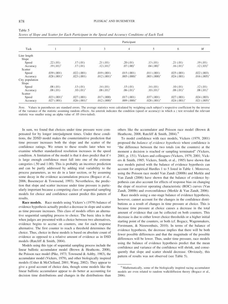
In sum, we found that choices under time pressure were com-pensated for by longer interjudgment times. Under these condi-tions, the 2DSD model makes the counterintuitive prediction thattime pressure increases both the slope and the scatter of theconfidence ratings. We return to these results later when weexamine whether standardized resolution increases in the speedcondition. A limitation of the model is that it does predict that if �is large enough confidence must fall into one of the extremecategories (.50 and 1.00). This is probably an incorrect predictionand can be partly addressed by adding trial variability to theprocess parameters, as we do in a later section, or by assumingsome decay in the evidence accumulation process (Bogacz et al.,2006; Busemeyer & Townsend, 1993). Nevertheless, the predic-tion that slope and scatter increase under time pressure is partic-ularly important because a competing class of sequential samplingmodels for choice and confidence cannot predict this pattern ofresults.

Race models. Race models using Vickers’s (1979) balance ofevidence hypothesis actually predict a decrease in slope and scatteras time pressure increases. This class of models offers an alterna-tive sequential sampling process to choice. The basic idea is thatwhen judges are presented with a choice between two alternatives,evidence begins to accrue on counters, one for each responsealternative. The first counter to reach a threshold determines thechoice. Thus, choice in these models is based on absolute count ofevidence as opposed to a relative amount of evidence as in DSDmodels (Ratcliff & Smith, 2004).

Models using this type of sequential sampling process include thelinear ballistic accumulator model (Brown & Heathcote, 2008),the Poisson race model (Pike, 1973; Townsend & Ashby, 1983), theaccumulator model (Vickers, 1979), and other biologically inspiredmodels (Usher & McClelland, 2001; Wang, 2002). They appear togive a good account of choice data, though some models like thelinear ballistic accumulator appear to do better at accounting fordecision time distributions and changes in the distributions than

others like the accumulator and Poisson race model (Brown &Heathcote, 2008; Ratcliff & Smith, 2004).9

To model confidence with race models, Vickers (1979, 2001)proposed the balance of evidence hypothesis where confidence is“the difference between the two totals (on the counters) at themoment a decision is reached or sampling terminated” (Vickers,2001, p. 151). Vickers and colleagues (Vickers, 1979, 2001; Vick-ers & Smith, 1985; Vickers, Smith, et al., 1985) have shown thatrace models paired with the balance of evidence hypothesis canaccount for empirical Hurdles 1 to 5 listed in Table 1. Moreover,using the Poisson race model Van Zandt (2000b) and Merkle andVan Zandt (2006) have shown that the balance of evidence hy-pothesis can also account for effects of response bias on changingthe slope of receiver operating characteristic (ROC) curves (VanZandt, 2000b) and overconfidence (Merkle & Van Zandt, 2006).

Race models using a one-stage balance of evidence hypothesis,however, cannot account for the changes in the confidence distri-butions as a result of changes in time pressure at choice. This isbecause time pressure at choice causes a decrease in the totalamount of evidence that can be collected on both counters. Thisdecrease is due to either lower choice thresholds or a higher initialstarting point of the counters, or both (cf. Bogacz, Wagenmakers,Forstmann, & Nieuwenhuis, 2010). In terms of the balance ofevidence hypothesis, the decrease implies that there will be bothfewer possible differences and that the magnitude of the possibledifferences will be lower. Thus, under time pressure, race modelsusing the balance of evidence hypothesis predict that the meanconfidence and variance of the confidence will shrink, and conse-quently that slope and scatter should decrease. Obviously, thispattern of results was not observed (see Table 5).

9 Mathematically, some of the biologically inspired racing accumulatormodels are even related to random walk/diffusion theory (Bogacz et al.,2006).

Table 5Scores of Slope and Scatter for Each Participant in the Speed and Accuracy Conditions of Each Task

Task

Participant

1 2 3 4 5 6 M

Line lengthSlope

Speed .22 (.01) .17 (.01) .21 (.01) .20 (.01) .13 (.01) .21 (.01) .19 (.01)Accuracy .19 (.01)� .17 (.01) .12 (.01)� .07 (.00)� .04 (.00)� .16 (.01)� .12 (.03)�

ScatterSpeed .039 (.001) .022 (.001) .019 (.001) .015 (.001) .011 (.001) .025 (.001) .022 (.003)Accuracy .028 (.001)� .023 (.001) .012 (.001)� .005 (.000)� .003 (.000)� .024 (.001) .016 (.005)�

City populationSlope

Speed .08 (.01) .13 (.01) .14 (.01) .15 (.01) .14 (.01) .10 (.01) .12 (.01)Accuracy .08 (.01) .10 (.01)� .08 (.01)� .06 (.01)� .10 (.01)� .08 (.01)� .08 (.01)�

ScatterSpeed .023 (.001)� .027 (.001) .017 (.000) .017 (.001) .037 (.001) .027 (.001) .024 (.003)Accuracy .027 (.001) .026 (.001)� .012 (.000)� .009 (.000)� .028 (.001)� .024 (.001)� .021 (.005)�

Note. Values in parentheses are standard errors. The average statistics were calculated by weighting each subject’s respective coefficient by the inverseof the variance of the statistic assuming random effects. An asterisk indicates the condition (speed or accuracy) in which a z test revealed the relevantstatistic was smaller using an alpha value of .05 (two-tailed).


A second stage of processing could be adopted in race models toaccount for these results. For instance, Van Zandt and Maldonado-Molina (2004) have developed a two-stage Poisson race model.However, we point out that the Poisson race model has severalother difficulties it must overcome. For instance, the model hasdifficulty in accounting for distributions of decision times (Ratcliff& Smith, 2004).10 There are other race models that might be bettercandidates for the two-stage balance of evidence hypothesis, in-cluding Brown and Heathcote’s (2008) linear ballistic accumulatorand Usher and McClelland’s (2001) leaky accumulator model. Weleave a full model comparison with these models for future inves-tigation. Next we examine several new quantitative predictions2DSD makes. To do so it is useful to fit the 2DSD model to themultivariate distribution of choice, decision time, and confidence.

Fit of 2DSD Interrogation Model to Choices, DecisionTimes, and Confidence Ratings

Model estimation. We fit the 2DSD interrogation model tothe distributions of choices, decision times, and confidence ratings.To do so we adapted Heathcote, Brown, and Mewhort’s (2002)quantile maximum probability (QMP) estimation method to simul-taneously fit the multivariate distribution of choice by decisiontime by confidence ratings (see also Speckman & Rouder, 2004).The general idea of QMP is to summarize the distribution ofdecision times in terms of quantiles. For example, we used quan-tiles of .1, .3, .5 .7, and .9. These estimated quantiles divide theobserved distribution of decision times into bins (e.g., six bins)with a number of observations within each bin (e.g., .1 � n in thefirst bin and .2 � n in the second bin, etc.). If the decision timeswere the only variable to be fit then the cumulative distributionfunction of DSD (see Appendix A) could be used to fit the modelto the observed number of observations within each quantile bin.This can be done for the correct and incorrect distributions ofdecisions times to obtain parameter estimates of the model.

The QMP method can be easily adapted to include confidenceratings. In our case, instead of six bins of observations the datarepresentation is a 6 (decision time categories) � 6 (confidenceratings) data matrix for corrects and incorrects for both tasks. Wefit the 2DSD interrogation model to this data representation with amultinomial distribution function using probabilities generated bythe 2DSD interrogation model. This was done for both the linelength and city population discrimination tasks. The models werefit at the individual level.

In both the line length and city population tasks we broke thedata down into two levels of time pressure crossed with differentlevels of difficulty. Recall, during the line length discriminationtask, within each time pressure condition, participants saw each ofthe six different comparisons 480 times. Unfortunately, all partic-ipants were extremely accurate with the sixth and easiest compar-ison (35.15 mm vs. a 32 mm standard). They scored 94% correctin speed and 98% correct in accuracy in this condition, producingvery few incorrect trials. As a result we collapsed the sixth andfifth levels of difficulty for both speed and accuracy, forming fivelevels of difficulty in the line length task to model. Representingthe line length discrimination data in terms of our adapted QMPmethod, each condition had 71 free data points producing a total of71 � 10 conditions (2 time pressure levels � 5 levels of diffi-culty) � 710 data points per participant. In the city population

task, based on the relationship between the cognitive performancevariables and the rank difference between city populations withineach pair (see Table 4), we formed six different levels of difficultywith approximately 300 pairs in each condition. Thus, the citypopulation task with 12 conditions (speed vs. accuracy � 6 levelsof difficulty) had 71 � 12 � 852 free data points per participant.

Trial variability and slow and fast errors. To better accountfor the data, we incorporated trial-by-trial variability into some ofthe process parameters of 2DSD. In particular, DSD models withno starting point bias (z � 0) and without trial variability predictthat the distribution for correct and incorrect choices should beequal (Laming, 1968; Link & Heath, 1975; Ratcliff & Rouder,1998; Ratcliff et al., 1999; Townsend & Ashby, 1983). Empiricallythis is not observed. Slow errors are often observed especiallywhen accuracy is emphasized during more difficult conditions.Slow errors have become an important hurdle for any model ofdecision times to overcome (Estes & Wessel, 1966; Luce, 1986;Swensson, 1972; Townsend & Ashby, 1983). We have added theresult of slow errors as the sixth empirical hurdle in Table 1 thatany complete model of cognitive performance must explain.Sometimes during the easier conditions—especially when timepressure is high—the opposite pattern of decision times is presentwhere the mean decision time for incorrect choices is faster thanthe mean decision time for correct choices (Ratcliff & Rouder,1998; Swensson & Edwards, 1971; Townsend & Ashby, 1983).We have also added this result to Table 1 as Hurdle 7.

These two hurdles—slow errors for difficult conditions (Hurdle6) and fast errors for easy conditions (Hurdle 7)—are problematicfor many sequential sampling models to explain. Ratcliff andcolleagues have shown that in order to simultaneously account forthis pattern of results DSD requires trial-by-trial variability in theprocess parameters (Ratcliff & Rouder, 1998; Ratcliff & Smith,2004; Ratcliff et al., 1999). Trial-by-trial variability in processingstimuli is an often-made assumption in stochastic models. This istrue not only for DSD but also Thurstonian scaling (Thurstone,1927) and signal detection theory (Green & Swets, 1966; Wallsten& Gonzalez-Vallejo, 1994). In terms of DSD and 2DSD onesource of trial variability, perhaps due to lapses in attention orvariability in memory processes (Pleskac, Dougherty, Rivadeneira,& Wallsten, 2009), is in the quality of the evidence accumulated orthe drift rate �. In particular, we assume that the drift rate forstimuli in the same experimental condition is normally distributedwith a mean � and a standard deviation �. Variability in the driftrate across trials causes the diffusion model to predict slowerdecision times for incorrect choices than for correct choices (Hur-dle 6; Ratcliff & Rouder, 1998).

A second source of trial variability is in the starting point (z).This assumption captures the idea that perhaps due to sequentialeffects from trial to trial judges do not start their evidence accu-

10 The basic problem is that although the distribution of decision timesbecomes more positively skewed as difficulty increases (Ratcliff & Smith,2004), the Poisson counter model tends to predict more symmetricaldistributions. Moreover, in the Poisson race model evidence is accumulatedin discrete evidence counts, which in turn means confidence is a discretevariable as well. This causes problems because best fitting parameters oftenresult in confidence having fewer than six possible values. Yet, confidencescales can easily have more than six values (e.g., when confidence is ratedin terms of probabilities).


mulation at the same state of evidence. In DSD and 2DSD thisvariability is modeled with a uniform distribution mean z andrange sz. Variability in the starting point across trials leads DSD topredict faster decision times for incorrect choices than for correctchoices, especially when speed is emphasized (Ratcliff & Rouder,1998; Ratcliff et al., 1999). Although this pattern is not stronglypresent in our data, we have also included this assumption of trialvariability in the starting point when fitting the 2DSD interrogationmodel.

A complete description of the 2DSD interrogation model pa-rameters is given in Table 2. For each decision task, we fit a highlyconstrained model to each participant’s data. Except where explic-itly noted, all parameters were fixed across conditions. Further-more, no systematic response bias was assumed so that the distri-bution of starting points was centered at z � 0 and the choicethresholds were set equal to � � �A � �B (recall the lowerthreshold is then ��). Across the different levels of difficulty onlythe mean drift rate � was allowed to vary. Thus, for each partici-pant there were five mean drift rates � for the line length task andsix �s in the city population task. For both decision tasks only thechoice thresholds � were allowed to vary between the two timepressure conditions. As an estimate of � we used the observedmean interjudgment time for the particular condition, corrected forany non-judgment-related processing time tEJ. With six confidenceratings (.50, .60, .70, .80, .90, and 1.00) there are five confidencecriteria. The confidence criteria were also fixed across experimen-tal conditions and were symmetrical for RA or RB response (e.g.,cRB,k � �cRA,k). Thus, in the line length task the 2DSD interrogationmodel had a total of 16 free parameters to account for 710 datapoints per participant. In the city population task there were a totalof 17 free parameters to account for 852 data points per partici-pant.11 The estimated parameters for each person and task areshown in Table 6.

To evaluate the fit of the 2DSD interrogation model we adaptedthe latency-probability function plots first used by Audley andPike (1965) to include confidence as well. We call the plotslatency–confidence–choice probability (LCC) functions. Figure 2shows the plots for the average participant during the line lengthtask (top row) and the corresponding plots for the city populationtask (bottom row). Overall each LCC function can be understoodas a plot showing how the measures of cognitive performancechange with stimulus discriminability. Within each figure, thelower half of the figure plots the mean decision times againstthe choice probability for correct choices (gray circles right ofchoice probability .5) and incorrect choices (white circles left ofchoice probability .5) for each level of difficulty. Because thesequential sampling models were fit to five levels of difficulty inthe line length task there are five correct (gray) and five incorrect(white) circles. In the city population task there are six correct(gray) and six incorrect (white) dots. The gray dot furthest to theright in each panel corresponds to the choice proportion andcorresponding decision time for the easiest condition. In otherwords, it has the highest choice probability and typically the fastestdecision time among corrects. The gray dot closest to the .5 choiceprobability corresponds to the proportion correct in the mostdifficult condition and the slowest average decision time amongcorrects. The white dots are configured similarly for incorrectchoices with the easiest condition on the far left. The upper portionof each panel plots the mean confidence against the choice prob-

ability in the same fashion. The solid lines marked with squarescorrespond to the predicted functions for the 2DSD interrogationmodel. Recall that although the LCC functions plot the means, themodels were fit using the quantiles of the decision times.

In terms of confidence, consistent with the slope scores, theobserved average confidence rating for corrects is greater than forincorrects. Furthermore, this difference between the confidenceratings (slope) increases as the stimuli get easier (moving out fromthe confidence-choice probability functions). This is true forboth the line length (top row) and city population (bottom row)tasks. The 2DSD model gives a good account of this trend.Furthermore, the LCC functions also show that the positive sloperelating confidence and accuracy was greater for the speed condi-tion compared to the accuracy condition. The 2DSD model repro-duces this change in slope. As discussed earlier, 2DSD attributesthe change in confidence with changes in difficulty to changes inthe mean drift rate, whereas the changes between time pressureconditions are attributed to an interaction between the interjudgmenttime and choice thresholds. The LCC functions do reveal that themodel tends to underestimate the mean confidence for incorrectchoices. One way to correct for this underestimation is to assumeseparate confidence criteria for correct and incorrect choices—weassumed symmetry to keep the model as simple as possible.

With respect to mean decision time, Figure 2 shows that al-though the model captures the pattern of changes across condi-tions, there is a constant discrepancy between the predicted andobserved mean times for the speed conditions. Under the con-straints used to fit the 2DSD model, the predicted time systemat-ically overestimates the observed time under the speed conditionsby an approximately constant amount. This is very likely causedby our assumption that the residual motor time, tED, is equal forspeed and accuracy conditions. This constant error could be fixedby allowing a smaller residual time constant for the speed condi-tions.

The LCC functions show that slow errors occurred where deci-sion times were slower for errors than correct responses for thecorresponding level of difficulty. Consistent with Hurdle 6, theslow errors are especially evident when accuracy was emphasizedand during the more difficult conditions. The 2DSD interrogationmodel with trial variability in the drift rate helps 2DSD account forthis pattern of slow errors. Without trial variability the modelpredicts identical decision time distributions for correct and incor-rect choices (assuming no bias) and the decision times in the LCCwould be a symmetrical inverted U shape.

Trial variability in 2DSD also helps account for other phenom-ena. In particular, trial variability in the drift rate helps account forthe observed relationship between confidence and decision timeseven when stimulus difficulty is held constant. Past studies (Baran-ski & Petrusic, 1998; Henmon, 1911) have indicated that evenwhen the stimulus difficulty is held constant (i.e., responding torepeated trials of the same line pairs) there is a negative relation-ship between decision time and confidence so that the fastest

11 We did not incorporate trial variability into the nondecision timecomponent tED. Nor did we incorporate so-called contaminant probabilityparameters that account for the small proportion of trials in which judgeshave a delay in their decision time. Both of these parameters have beenused in other diffusion models (Ratcliff & Tuerlinckx, 2002).


decision times are generally associated with the highest confidencerating. Indeed participants in the line length task tended to showthis pattern of results. Table 7 lists the average Goodman andKruskal � rank–order correlation between decision time and con-fidence for each participant in the line length task holding stimulusdifficulty constant. These correlations reveal that for nearly every-one, holding stimulus difficulty constant, there was a negativecorrelation between decision time and confidence and the strengthof this relationship was strongest for correct responses during theaccuracy conditions.

The 2DSD model (without trial variability) predicts that for agiven stimulus, decision times and confidence are independent ofeach other (separately for correct and incorrect choices). The2DSD model with trial variability attributes this relationship be-tween confidence and decision time to trial-by-trial variability inthe drift rate. That is, even when stimulus discriminability is heldconstant there is a negative relationship between decision time andconfidence (Hurdle 4 in Table 1) because from trial to trial thereare fluctuations in the processing of the same stimuli that lead tochanges in the quality of the evidence being accumulated. On sometrials when the quality of the evidence extracted from a stimulus ishigh the drift rate will be high and lead to fast decision times andhigh levels of confidence. On other trials when the quality of theevidence is low the drift rate will be low and lead to slow decisiontimes and lower levels of confidence. The model does, however,underestimate the relationship between observed decision time andconfidence. For example, as listed in Table 7, the average observedGoodman and Kruskal �s between decision time and confidenceacross participants and difficulty levels were –.21 and –.39 forcorrect choices in speed and accuracy conditions, respectively. Theaverage predicted correlations generated from the best fittingmodel parameters for each participant for the speed and accuracyconditions were –.10 and –.15, respectively. Nevertheless, this

result provides further support for the necessity of including trialvariability in the process parameters to give a full account of thedata.

Accuracy of Confidence Ratings

So far we have shown the 2DSD model can explain the differ-ences in confidence for speed and accuracy conditions by thelonger interjudgment time that the judges used under the speedcondition. But why did they do this? An answer to this questioncomes from understanding how the time course of the judgmentprocess impacts the accuracy of confidence judgments. In thissection we first describe some of the basic measures of confidenceaccuracy and examine the predictions of the 2DSD model for thesemeasures. Then we examine the question of how to optimize bothchoice and confidence accuracy under time pressure conditions.

Confidence is useful not only in the lab to help chart cognitiveprocesses but also outside of the lab where it is often communi-cated as a subjective probability that an event has occurred or willoccur (Adams & Adams, 1961; de Finetti, 1962; Savage, 1954).An important and well-studied aspect of subjective probabilities istheir accuracy (see Arkes, 2001; Griffin & Brenner, 2004; Koehler,Brenner, & Griffin, 2002; McClelland & Bolger, 1994). The focuson accuracy is well-deserved. Every day many important decisionsare made using subjective probabilities to weigh the costs andbenefits of the consequences of those decisions. Yet, very little isknown about how time pressure affects the time allocation formaking both choices and confidence ratings. In fact, 2DSD can beused to address this problem. To do so it is easier to rely on the2DSD interrogation model. As we have shown, the 2DSD inter-rogation model by treating interjudgment time as an exogenousparameter captures all of the critical phenomena regarding therelationship between choice, decision time, and confidence.

Table 6Parameter Estimates for Each Participant From the 2DSD Interrogation Model With Trial Variability in the Drift Rateand Starting Point

Parameter

Participants in line length task Participants in city population task

1 2 3 4 5 6 M 1 2 3 4 5 6 M

�1 .0521 .0375 .0261 .0322 .0372 .0389 .0373 .0118 .0239 .0205 .0181 .0170 .0158 .0179�2 .1267 .1032 .0759 .0781 .1112 .0871 .0970 .0234 .0456 .0430 .0435 .0533 .0346 .0406�3 .2171 .1961 .1418 .1661 .1969 .1544 .1787 .0276 .0739 .0627 .0809 .0697 .0554 .0617�4 .2762 .2578 .1890 .2308 .2472 .2473 .2414 .0506 .0989 .0757 .1036 .0977 .0856 .0854�5 .3527 .3719 .2655 .3446 .3189 .3762 .3383 .0565 .1497 .0968 .1477 .1259 .1348 .1186�6 .0952 .2264 .1476 .2070 .2168 .1991 .1820� .1477 .1757 .0876 .1292 .0930 .1583 .1319 .0484 .1295 .0662 .1085 .1419 .1532 .1080�speed .0634 .0490 .0455 .0463 .0536 .0493 .0512 .0679 .0674 .0857 .0699 .0834 .0741 .0747�acc .0854 .0770 .0932 .1722 .0797 .1440 .1086 .0908 .1141 .1570 .2125 .2013 .1958 .1619sz .0580 .0281 .0110 .0378 .0312 .0000 .0277 .0430 .0391 .0000 .0440 .0411 .0000 .0279tED .3234 .3747 .2920 .4084 .3240 .3966 .3532 .4510 .7847 .4590 .7289 .5579 .7709 .6254tEJ .0660 .0000 .0009 .0000 .0000 .0000 .0112 .0000 .0000 .0000 .0000 .0000 .0000 .0000c1 .0750 �.0143 �.0713 �.0956 �.0193 .0706 �.0092 .1325 .0210 �.0199 �.1075 .1147 .0809 .0370c2 .1066 .0543 �.0024 �.0068 �.0193 .1501 .0471 .1714 .0967 .0518 .0179 .1570 .2226 .1196c3 .1157 .1251 .0491 .0509 �.0193 .2151 .0894 .1851 .1553 .1061 .1370 .1936 .3256 .1838c4 .1241 .1739 .0691 .1038 �.0193 .2861 .1230 .1942 .2042 .1817 .2255 .2274 .4275 .2434c5 .1482 .2125 .1095 .2126 �.0145 .3595 .1713 .1998 .2499 .2140 .2877 .2506 .5386 .2901

Note. 2DSD � two-stage dynamic signal detection; � � mean value of the drift rate between trials; � � standard deviation of the drift rate between trials;�speed and �acc � choice thresholds for speed and accuracy, respectively; sz � range of starting points; tED � mean nondecision time; tEJ � meannonjudgment time; c1–c5 � confidence criteria.


Substantive goodness. There are, in fact, two different di-mensions by which the accuracy of subjective probability estimatecan be evaluated: substantively and normatively (Winkler & Mur-phy, 1968). Substantive goodness captures the idea that forecastersshould be able to distinguish between events that occur or not withtheir confidence estimates (resolution). In other words, do confi-dence ratings reflect whether the judge has made a correct choice?

The slope (difference between the mean confidence rating forcorrect choices and the mean confidence rating for incorrectchoices) is one measure of substantive goodness (Yates, 1990;Yates & Curley, 1985). As we showed in the present study, theslope scores increased under time pressure in both perceptual andgeneral knowledge tasks (see Table 5). This increase in slope isindicative of a resolution in confidence about the accuracy of theirdecision under time pressure at choice. 2DSD attributes this en-hanced resolution to the increase in evidence collection, whether itis with an increase in interjudgment times � in the interrogationmodel or a decrease in exit probabilities w in the optional stoppingmodel (the optional stopping model is described in full later).

Recall also that this increase in slope is paired with—as 2DSDgenerally predicts—an increase in scatter or the pooled variance ofconfidence across correct and incorrect choices (see Table 5). Thisincrease in scatter (i.e., greater variance) may detract from theincrease in slope (i.e., mean difference) in terms of a judge’sresolution (Wallsten, Budescu, Erev, & Diederich, 1997; Yates &Curley, 1985). To examine this question we calculated a standard-ized measure of resolution called DI� (Wallsten et al., 1997),

DI� �slope

�scatter. (18)

Table 8 lists the means and standard deviations of the DI� scoresacross participants in each task (individual estimates can calcu-

.00 .25 .50 .75 1.000.450

0.525

0.600

Speed

Lin

e Le

ngth

Dec

isio

n T

ime

t D’(s

)

.50

.60

.70

.80

.90

1.00

.00 .25 .50 .75 1.000.400

1.400

2.400

Accuracy

.50

.60

.70

.80

.90

1.00

Con

fiden

ce

.00 .25 .50 .75 1.000.800

1.000

1.200

Choice Prob.Incorrect Correct

City

Pop

ulat

ion

D

ecis

ion

Tim

e t D

’(s)

.50

.60

.70

.80

.90

1.00

.00 .25 .50 .75 1.000.900

2.450

4.000

Choice Prob.Incorrect Correct

.50

.60

.70

.80

.90

1.00

Con

fiden

ce

Figure 2. The latency–confidence–choice probability functions for the average participant during the linelength (top row) and city population (bottom row) discrimination tasks. The best fitting functions for thetwo-stage dynamic signal detection (2DSD) interrogation model with trial variability in the starting point anddrift rate are shown. The circles with dashed lines are the data, and the squares with solid lines are the fits ofthe 2DSD model. Unshaded markers are the error or incorrect responses; shaded markers are the correctresponses. The error bars represent �1.96 SE.

Table 7Average Goodman and Kruskal � Between Confidence andDecision Time Holding Difficulty Constant for the Line LengthTask for Each Participant

Condition

Participant

1 2 3 4 6 M

SpeedCorrect �.25� �.34� .01 �.21� �.29� �.21�

Incorrect �.08 �.27� .07 .11 �.15� �.07Accuracy

Correct �.35� �.33� �.30� �.54� �.50� �.39�

Incorrect �.12 �.25� .02 �.21 �.30� �.18�

Note. Participant 5 used primarily the .50, .90, and 1.00 confidenceratings during the line discrimination task and was thus excluded fromthese calculations.� p � .05, two-tailed.


lated using the values in Table 5). Using DI� as an index ofresolution, we still see an increase in resolution during the speedconditions of both tasks.12 Baranski and Petrusic (1994) reporteda similar result. This increase in standardized resolution is bestunderstood within the context of the 2DSD interrogation model.Recall in general that in DSD standardized accuracy grows as alinear function of the square root of time (e.g., �; see Equation 5).This finding (increased resolution in confidence judgments whenfacing time pressure at choice but not during confidence rating) isadded as the eighth and final empirical hurdle any model mustexplain (see Table 1). Race models using a one-stage balance ofevidence hypothesis do not clear this empirical hurdle.

Normative goodness. The second dimension of the accuracyof subjective probabilities is normative goodness. Normativegoodness addresses the idea that when confidence ratings come inthe form of subjective probabilities, we also demand them toadhere to the properties of probabilities. This adherence is becausedecision makers use subjective probability judgments, like thelikelihood of rain tomorrow or the probability that a sports teamwill win, to weigh the costs and benefits of different outcomes inmaking a variety of decisions. Thus, confidence ratings whengiven as subjective probabilities should also be evaluated in termsof their normative goodness or how well they meet the demands ofprobabilities (Winkler & Murphy, 1968). We can further breaknormative goodness into coherence and correspondence. The firstfactor of normative goodness is coherence or the degree to whichestimates conform to the mathematical properties of probabilitiesspecified in the Kolmogorov axioms of probability (see e.g., Rot-tenstreich & Tversky, 1997; Tversky & Kahneman, 1974; Tversky& Koehler, 1994). For this article we focused on the second factorof correspondence or the degree of calibration between estimatedsubjective probabilities and the true probabilities of an eventoccurring. For example, if a judge says the probability he or she iscorrect is 75% then is he or she actually correct 75% of the time?Note that correspondence in subjective probability estimates im-plies coherence, but coherence does not imply correspondence.However, correspondence does not necessarily imply good reso-lution or substantive goodness. For example, a weather forecaster

who uses the long-run historical relative frequency of rain duringa particular month as his or her forecast might be well calibratedbut certainly does not have good resolution.

Participants in our study were generally overconfident in boththe line length and city population tasks. One measure of corre-spondence is the difference between the average confidence ratingand the proportion correct,

bias � conf � pc, (19)

where bias � 0 indicates overconfidence.13 That is, judges tend tooverestimate the likelihood they are correct. Table 8 lists themeans and standard deviations of the bias scores across partici-pants in the speed and accuracy conditions of both tasks (individ-ual estimates can calculated using the values in Table 3). The biasscores show that most participants were on average overconfidentin both the line length and city population tasks. Past results havesometimes found underconfidence in perceptual tasks like the linelength task and overconfidence in general knowledge tasks like thecity population task (Bjorkman, Juslin, & Winman, 1993; Dawes,1980; Keren, 1988; Winman & Juslin, 1993), though not always(Baranski & Petrusic, 1995). This divergence has sometimes beenunderstood as indicating separate and distinct choice/judgmentprocesses for perceptual and conceptual/general knowledge tasks(Juslin & Olsson, 1997; Juslin et al., 1995). We return to this twoversus one process argument in the discussion, but note that by andlarge 2DSD has provided an adequate account of the data in bothtasks, suggesting perhaps that the distinction between perceptualand conceptual tasks is more a difference in information ratherthan a difference in process.

Table 8 also shows that in general participants were slightlymore overconfident when they were under time pressure. Thesedifferences, however, are small. Using the statistics in Table 3 onecan see that the change in overconfidence arose because, forexample, in the line length task their proportion correct fell about7 percentage points when under time pressure but their confidenceonly decreased on average about 5 percentage points. A similarpattern emerged in the city population task where accuracy fellabout 7 percentage points whereas confidence only decreasedabout 4 percentage points.

Reliability diagrams or calibration curves are a useful way tovisualize the correspondence between stated confidence ratingsand the proportion of correct inferences. Calibration curves plotthe relative frequencies of an event occurring (correct choice) forgiven respective discrete forecasts (.50, .60, . . . , 1.00; Lichten-stein et al., 1982; Murphy & Winkler, 1977). Figure 3 shows thecalibration plot for the two different tasks for Participant 2. The

12 This increase in resolution in the speed conditions is evident even withGoodman and Kruskal’s ordinal measure of association � (see Table 4; seeNelson, 1984, 1987, for an argument as to the use of � as a primarymeasure of accuracy).

13 Another measure of overconfidence is the conf score (Erev et al.,1994), which is the weighted average difference between the stated con-fidence rating and the proportion correct across the different confidenceratings, excluding the .5 confidence rating. Due to the large sample sizes,the values for conf score as well as the same statistic including the .5response are very similar to the bias score statistic, and all conclusionsstated within the article are identical. We use the bias score due to itsrelationship with the Brier score, which we use in the next section.

Table 8DI�, Bias, and Brier Scores Across Participants in the Speedand Accuracy Conditions of Each Task

Variable

Line length City population

M SE SDbetween M SE SDbetween

DI�Speed 1.32 0.08 0.19 0.83 0.10 0.23Accuracy 0.99� 0.06 0.16 0.60� 0.04 0.09

BiasSpeed .08 .03 .07 .10 .03 .06Accuracy .05� .02 .06 .07� .03 .07

BrierSpeed .141 .005 .012 .209 .005 .013Accuracy .113� .006 .014 .191� .011 .026

Note. DI� and Brier score standard errors were estimated with a bootstrapmethod. An asterisk indicates the condition (speed or accuracy) in which az test revealed the relevant statistic was smaller using an alpha value of .05(two-tailed).


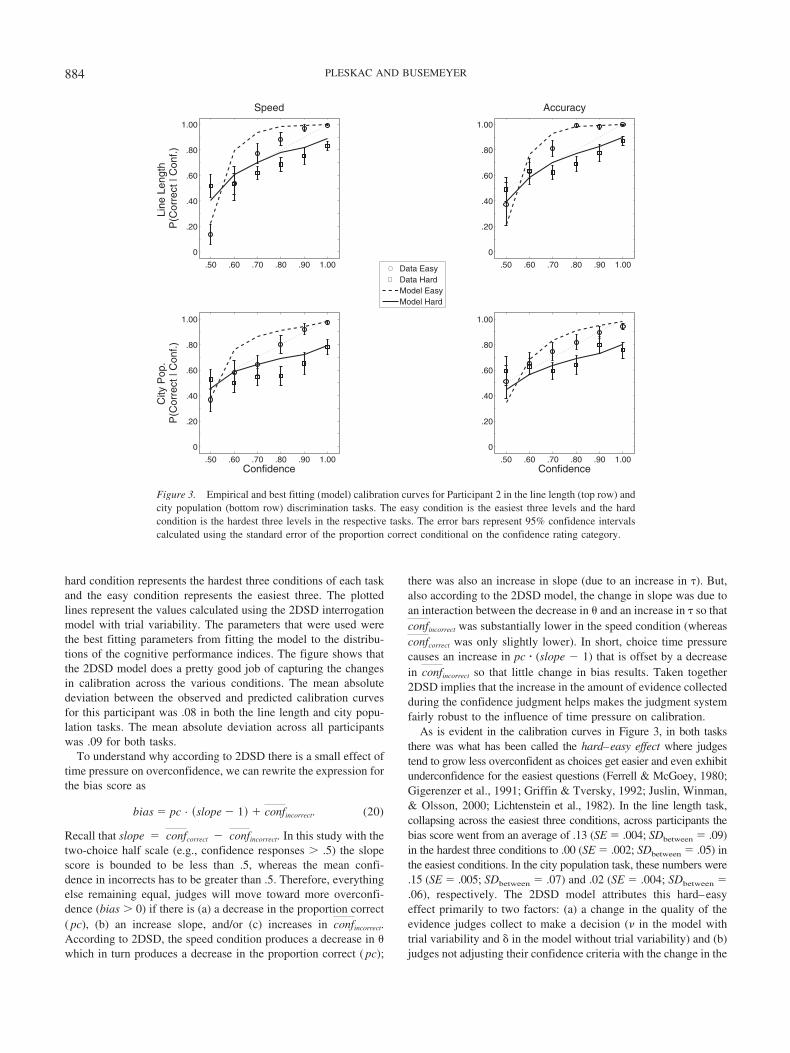
hard condition represents the hardest three conditions of each taskand the easy condition represents the easiest three. The plottedlines represent the values calculated using the 2DSD interrogationmodel with trial variability. The parameters that were used werethe best fitting parameters from fitting the model to the distribu-tions of the cognitive performance indices. The figure shows thatthe 2DSD model does a pretty good job of capturing the changesin calibration across the various conditions. The mean absolutedeviation between the observed and predicted calibration curvesfor this participant was .08 in both the line length and city popu-lation tasks. The mean absolute deviation across all participantswas .09 for both tasks.

To understand why according to 2DSD there is a small effect oftime pressure on overconfidence, we can rewrite the expression forthe bias score as

bias � pc · �slope � 1� � confincorrect. (20)

Recall that slope � confcorrect � confincorrect. In this study with thetwo-choice half scale (e.g., confidence responses � .5) the slopescore is bounded to be less than .5, whereas the mean confi-dence in incorrects has to be greater than .5. Therefore, everythingelse remaining equal, judges will move toward more overconfi-dence (bias � 0) if there is (a) a decrease in the proportion correct( pc), (b) an increase slope, and/or (c) increases in confincorrect.According to 2DSD, the speed condition produces a decrease in �which in turn produces a decrease in the proportion correct ( pc);

there was also an increase in slope (due to an increase in �). But,also according to the 2DSD model, the change in slope was due toan interaction between the decrease in � and an increase in � so thatconfincorrect was substantially lower in the speed condition (whereasconfcorrect was only slightly lower). In short, choice time pressurecauses an increase in pc � (slope � 1) that is offset by a decreasein confincorrect so that little change in bias results. Taken together2DSD implies that the increase in the amount of evidence collectedduring the confidence judgment helps makes the judgment systemfairly robust to the influence of time pressure on calibration.

As is evident in the calibration curves in Figure 3, in both tasksthere was what has been called the hard–easy effect where judgestend to grow less overconfident as choices get easier and even exhibitunderconfidence for the easiest questions (Ferrell & McGoey, 1980;Gigerenzer et al., 1991; Griffin & Tversky, 1992; Juslin, Winman,& Olsson, 2000; Lichtenstein et al., 1982). In the line length task,collapsing across the easiest three conditions, across participants thebias score went from an average of .13 (SE � .004; SDbetween � .09)in the hardest three conditions to .00 (SE � .002; SDbetween � .05) inthe easiest conditions. In the city population task, these numbers were.15 (SE � .005; SDbetween � .07) and .02 (SE � .004; SDbetween �.06), respectively. The 2DSD model attributes this hard–easyeffect primarily to two factors: (a) a change in the quality of theevidence judges collect to make a decision (� in the model withtrial variability and � in the model without trial variability) and (b)judges not adjusting their confidence criteria with the change in the

.50 .60 .70 .80 .90 1.00

0

.20

.40

.60

.80

1.00

Li

ne L

engt

h

P(C

orre

ct |

Con

f.)

Speed

Data EasyData HardModel EasyModel Hard

.50 .60 .70 .80 .90 1.00

0

.20

.40

.60

.80

1.00

C

ity P

op.

P

(Cor

rect

| C

onf.)

Confidence

.50 .60 .70 .80 .90 1.00

0

.20

.40

.60

.80

1.00

Accuracy

.50 .60 .70 .80 .90 1.00

0

.20

.40

.60

.80

1.00

Confidence

Figure 3. Empirical and best fitting (model) calibration curves for Participant 2 in the line length (top row) andcity population (bottom row) discrimination tasks. The easy condition is the easiest three levels and the hardcondition is the hardest three levels in the respective tasks. The error bars represent 95% confidence intervalscalculated using the standard error of the proportion correct conditional on the confidence rating category.


quality of the evidence (for a similar argument see Ferrell &McGoey, 1980; Suantak et al., 1996).

Overall accuracy. Now we return to the main question thatpermeates all of these analyses: Why did participants respond tochanges in time pressure by increasing the amount of evidencethey collect during the second stage of processing? Intuitively, thereaction of participants seems sensible. When forced to make achoice under time pressure, it seems reasonable to take a bit longerand collect more evidence to assess one’s confidence in thatchoice. In fact, using 2DSD we can also see that this reaction is atleast consistent with an optimal solution where judges seek tominimize decision and interjudgment time as well as maximizechoice and confidence accuracy.

To derive this prediction, it is useful to measure choice andconfidence accuracy (or inaccuracy) with the Brier (1950) score,

brier � �confi � correcti�2. (21)

In this equation, correcti is equal to 1 if the choice on trial i wascorrect, otherwise 0, and confi was the confidence rating entered interms of probability of correct (.50, .60, . . . , 1.00). In this case thegoal of the judge is to produce judgments that minimize the Brierscore. The Brier score is a useful overall measure of accuracy fortwo reasons. One reason is that the Brier score is a strictly properscoring rule (Aczel & Pfanzagal, 1966; de Finetti, 1962; Murphy,1973; von Winterfeldt & Edwards, 1986; Yates, 1990). This meansthat if participants have an explicit goal of minimizing their Brierscore they will achieve this minimum if they (a) give an accuratechoice and (b) truthfully map their internal subjective belief thatthey are correct, p*, to the closest external probability valueavailable (conf). Recall that participants were rewarded in bothtasks according to a linear transformation of the Brier score (seeEquation 15). Thus, it was in participants’ best interests to have agoal of minimizing their Brier score.

A second reason the Brier score is useful is that the mean Brierscore can be decomposed in the following manner:

brier � VI � bias2 � �VI��slope��slope � 2� � scatter,

(22)

(Yates, 1990; Yates & Curley, 1985) and for a similar decompo-sition, see Murphy (1973). In the above equation, VI or thevariability index is set to VI � p(correct)p(incorrect). Thus, ac-cording to this decomposition, the Brier score integrates choiceaccuracy, normative goodness, and substantive goodness (cf. Win-kler & Murphy, 1968).

Table 8 lists the average Brier score under speed and accuracyinstructions for both the line length and city population discrimi-nation tasks. The standard error for the average Brier score wasestimated using bootstrap methods. By and large, participantstended to have worse (higher) Brier scores in the speed conditions.Not listed in the table is the effect of difficulty on the Brier score.Predictably, the Brier score was also influenced by difficulty. Inthe line length task the average Brier score was .211 (SE � .065;SDbetween � .021) in the hardest three conditions, which wassignificantly larger than the average Brier score in the easiest threeconditions, .045 (SE � .019; SDbetween � .006). In the city pop-ulation task, the average Brier score was .260 (SE � .029;

SDbetween � .019) in the hardest three conditions, which wassignificantly larger than the average Brier score in the easiest threeconditions, .142 (SE � .023; SDbetween � .033).

Using the Brier score decomposition in Equation 22 we can seehow changes in different types of accuracy lead to changes in theBrier score. For example, a decrease in choice accuracy will byand large increase the mean Brier score via the variability index.But, an increase in slope will decrease the Brier score (the deriv-ative of Equation 22 with respect to slope is negative). Accordingto 2DSD when judges increased the amount of evidence collectedduring the second stage of processing under time pressure atchoice they were at least in principle counteracting the negativeimpact of lower choice accuracy on the Brier score and their finalearnings. To investigate this claim we used the 2DSD interrogationmodel with trial variability to evaluate how the Brier score changesas a function of (a) choice thresholds � and (b) interjudgment times�. Figure 4 plots this relationship for Participant 3 in the citypopulation task. It shows that according to 2DSD the Brier scorewill decrease when choice thresholds are increased and/or wheninterjudgment times � are increased.14

But of course this change in choice thresholds and interjudg-ment times exacts some costs on the judge. In particular, theimprovement in overall accuracy comes at the cost of greaterprocessing time. A way to conceptualize these different demandsof accuracy and time is with the cost function

cost � c1 · t�D � c2 · �� c3 · brier, (23)

where c1, c2, and c3 specify the cost of the observed decision timet�D, the observed interjudgment time ��, and the level of a Brierscore, respectively.

Using 2DSD one can ask what response parameters for a givenstimulus or stimuli minimize the cost function in Equation 23. Inparticular, for the 2DSD interrogation model what choice thresh-olds (�), interjudgment times (�), and confidence criteria lead tothe smallest cost for a given set of costs? A closed-form solutiondoes not appear to be available to answer this question. However,the monotonic decreases in the Brier score with choice thresholdsand interjudgment times demonstrated in Figure 4 imply a uniquesolution can often be found. In particular if (a) judges seek tominimize their Brier score as the cost of decision time increases,and (b) face a constant level of cost for their interjudgment time,then judges should increase their interjudgment time to minimizethe total cost in Equation 23. That is, by taking more time forjudgment following a choice under the choice time pressure con-dition, participants in the line length and city population tasksacted in a manner consistent with the optimal solution for this task.

14 Note this relationship with the Brier score is dependent to somedegree on the location of the confidence criteria/markers and drift rate. Forexample, at extreme levels of drift rate/mean drift rate, changes in inter-judgment time and choice thresholds have little effect on the Brier score.Furthermore, the relationship also breaks down when judges use whatappear to be atypical locations of confidence criteria/markers (e.g., onlyusing the .50, .90, and 1.00 confidence ratings).


2DSD Optional Stopping Model Account ofInterjudgment Times

A new challenge for 2DSD. 2DSD posits a simple andstraightforward hypothesis: There is postdecision processing ofevidence, and judges use this extra evidence accumulation toassess their confidence in their choice. The 2DSD interrogationmodel captures this idea by supposing judges continue accu-mulating evidence for a fixed amount of time (i.e., interjudg-ment time �) after making a choice treating the interjudgmenttimes as an exogenous parameter of the model. In fact, when wefit the model we used the observed mean interjudgment time toestimate the interjudgment time � parameter in the model.Although the simplicity of the interrogation model is certainlya strength and as we have shown the model provides a goodaccount of the data, one unexplained result is the negativecorrelation between interjudgment times and confidence shownin Table 4. This negative relationship replicates similar resultsreported by Baranski and Petrusic (1998) and Petrusic andBaranski (2003; see also Van Zandt & Maldonado-Molina,2004). The 2DSD interrogation model (see Figure 1) does notexplicitly predict such a relationship.

The relationships between interjudgment times and the otherperformance-relevant variables in Table 4 suggest that interjudg-ment time is not an exogenous parameter of the judgment process,but rather endogenous to the process. The strongest relationship isthe negative relationship between the level of confidence and the

interjudgment times. This relationship between confidence andinterjudgment time has been interpreted as further evidence ofsome postdecisional computational processing (Baranski & Petru-sic, 1998; Petrusic & Baranski, 2003; Van Zandt & Maldonado-Molina, 2004).

2DSD can account for this relationship between interjudgment timeand confidence as well as the other associations detailed in Table 4 byassuming the stopping rule for a confidence judgment is an optional(rather than a fixed) stopping rule. In this case, during the second stageof evidence accumulation some standard internal to the judgmentsystem determines when a judge stops and makes a confidencejudgment (much like the choice threshold �). To formulate thisalternative stopping rule, it is useful to consider 2DSD as a Markovchain (e.g., Diederich & Busemeyer, 2003) as shown in Figure 5. Thetop chain describes a random walk choice process. The circles repre-sent different evidence states ranging from the lower choice threshold–� to the upper threshold �. Evidence is accumulated by adjusting thejudge’s evidence state up a step (�) with probability p or down astep (��) with probability q, where the probability p is determined bythe mean drift rate parameter �. The evidence states corresponding tothe choice thresholds (black circles) denote the typical absorbingbarriers in diffusion models (corresponding to the threshold parameter�). Once the process reaches one of the thresholds at the end of thechain, a choice is made accordingly. Using the Markov chain approx-imation, and by setting the step size sufficiently small (�), we cancalculate the relevant distribution statistics including choice probabil-

0.05 (0.69 s)

0.10 (1.29 s)

0.20 (3.08 s)

0.15 (2.11 s)

0

0.50 s

1.00 s

1.50 s

2.00 s

2.50 s

0.12

0.14

0.16

0.18

0.2

0.22

0.24

0.26

Choice Threshold θ (tD

’)Inter−Judgment Time τ’

Pre

dict

ed B

rier

Sco

re

Speed Conditionθ = 0.085; τ = 0.68 s

Pre. Brier = 0.19Obs. Brier = 0.20

Accuracy Conditionθ = 0.15; τ = 0.31 s

Pre. Brier = 0.17Obs. Brier = 0.17

Figure 4. Predicted Brier scores for Participant 3 in the city population task in Difficulty Level 3. The plot wascalculated using the two-stage dynamic signal detection (2DSD) interrogation model with trial variability in theparameters. The plot illustrates that according to the 2DSD model, increases in the choice threshold � andinterjudgment time � both minimize a person’s Brier score. This implies that the model can be used to findappropriate choice threshold and interjudgment time settings that produce the fastest total judgment time(choice confidence) for a given Brier score.


ities and decision times that closely approximate a continuous timediffusion process (see Appendix C; Diederich & Busemeyer, 2003).

More importantly for our interests, the discrete state space givesanother means to conceptualize our two-stage hypothesis. Under thisformulation, the confidence stage is modeled as a second Markovchain (see the bottom chain in Figure 4 when Alternative A is chosen).Now during the second stage of processing, we assume markers �j areplaced along the evidence state space representing the different con-fidence ratings (j � .50, .60, . . . , 1.00), one for each rating. For theintermediary confidence ratings (.60, .70, .80, and .90), each timeevidence passes one of these markers there is a probability wconf thatthe judge exits and gives the corresponding confidence rating.15 Theevidence states representing the confidence ratings of .50 and 1.00were set equal to an absorbing boundary (w.50 � w1.00 � 1.0, thus theblack circles shown in the lower chain in Figure 5). This means thatonce the process enters one of these extreme states then with proba-bility 1 the evidence accumulation process ends and the correspond-ing confidence rating is given. Using the same Markov chain methodsthat determine the choice and decision times, the distribution ofconfidence ratings and distribution of interjudgment times can becomputed (see Appendix C).

Fitting the 2DSD optional stopping model. Evaluating the2DSD optional stopping model is very challenging because itrequires simultaneously fitting the entire distribution of responsesacross choices, decision times, confidence ratings, and interjudg-ment times for the different conditions of each decision task.Appendix C describes the detailed procedures used to accomplishthe fits. In this section we summarize the most important points.To summarize the procedure, we fit quantiles averaged acrossindividuals, and this fit was done separately for each of the two

conditions of time pressure and decision task conditions.16,17 Eachtime pressure and decision task condition had approximately 81free data points, and the 2DSD optional stopping model had 14free parameters. The parameter estimates are shown in Table 8.18

The most important finding that needs to be explained with this2DSD optional stopping model is the relation between confidenceratings and interjudgment times. Figure 6 displays the quantiles(.1, .3, .5, .7, and .9) of the distribution of interjudgment times asa function of confidence and accuracy, averaged across all six

15 A similar procedure has been used to model the indifference responsein preferential choice using decision field theory (Busemeyer & Goldstein,1992; Busemeyer & Townsend, 1992; J. G. Johnson & Busemeyer, 2005).

16 Note this is a different approach than in the previous section where wefit the 2DSD interrogation model by constraining a majority of the param-eters to be constant across conditions. We chose to fit the full model to eachcondition to aid the optimization method in finding the best fitting param-eters. The parameter estimates we obtained (see Table 8) suggest that someof the model parameters can be held constant across conditions. Forexample, the drift rate for each time pressure condition in each decisiontask appears to change very little between conditions.

17 We collapsed across the different levels of difficulty to increase thenumber of observations per distribution of interjudgment times. Moreover,we averaged across participants because even with the high number ofobservations per subject some of the intermediary confidence levels had alow number of observations.

18 Although trial variability in process parameters (e.g., drift rate �) canbe included (see Diederich & Busemeyer, 2003) in this model, we did notincorporate this aspect of the model due to the computational limits offitting the model with the Markov approximation.

Figure 5. A Markov chain approximation of the two-stage dynamic signal detection (2DSD) optional stoppingmodel. In the model, evidence accumulates over time toward an upper (�) and lower (��) threshold. Thisaccumulation is approximated with discrete states in the model using probabilities p and q of moving a step size� to each adjacent state. This process can produce a trajectory such as the jagged line in Figure 1. After makinga choice, judges continue accumulating evidence but are assumed to lay out markers �j across the state space sothat if the process crosses through that particular state, judges exit with probability wj and give the correspondingconfidence rating. These markers are identified with gray and black dots in the bottom chain. To adequately fitthe data, the model assumed that the two extreme confidence ratings (e.g., .50 and 1.00) were associated withan absorbing boundary so that if the process entered its associated state the judge would stop accumulatingevidence and state the respective level of confidence. If Alternative B was chosen a similar chain is used (notshown), which is a reflection of the chain used if Alternative A was chosen. The model predicts at the distributionlevel choice, decision time, confidence, interjudgment times, and their interrelationships (see Appendix C). z �starting point.


participants, separately for each decision task and speed instructioncondition. In particular, the triangles display the median interjudg-ment time, which is largest when confidence is lowest and de-creases as confidence becomes more extreme.

Figure 6 also shows that by and large the model gives a goodaccount of the distributions. In particular, the model gives a goodaccount of the negative relationship between confidence and inter-judgment times. One property of the model that helps determine thisrelationship is the location of the confidence markers. For example,notice that in our data the .50 confidence rating had the slowest

interjudgment time. To capture this property the best fitting markerlocation for the .50 confidence rating �.50 was below the starting pointof the choice process of z � 0 in the evidence space (see Table 9).However sometimes there is a nonmonotonic relationship betweenconfidence and interjudgment times where the interjudgment timesassociated with guess (or .50 in our study) are slightly faster than theintermediary confidence ratings (Baranski & Petrusic, 1998; Petrusic& Baranski, 2003). The 2DSD optional stopping model could accountfor this by moving the �.50 marker up in the evidence space. Doing sowould lead to faster interjudgment times for this confidence rating.

1.00 .90 .80 .70 .60 .50 .50 .60 .70 .80 .90 1.000.000

0.500

1.000

1.500

2.000

2.500Speed

Lin

e Le

ngth

In

ter−

judg

men

t Tim

e τ’

(s)

Data .9

Data .7

Data .5

Data .3

Data .1

Model .9

Model .7

Model .5

Model .3

Model .1

1.00 .90 .80 .70 .60 .50 .50 .60 .70 .80 .90 1.000.000

0.500

1.000

1.500

2.000

2.500Accuracy

1.00 .90 .80 .70 .60 .50 .50 .60 .70 .80 .90 1.000.000

0.500

1.000

1.500

2.000

2.500

City

Pop

ulat

ion

Inte

r−ju

dgm

ent T

ime τ’

(s)

Confidence Incorrect Correct

1.00 .90 .80 .70 .60 .50 .50 .60 .70 .80 .90 1.000.000

0.500

1.000

1.500

2.000

2.500

Confidence Incorrect Correct

Figure 6. Observed and best fitting (model) distribution of interjudgment times (�) as a function of confidenceand accuracy in the line length and city population tasks for the average participant. The observed and best fittingdistributions are plotted using the .1, .3, .5, .7, and .9 quantiles of the respective distributions. The best fittingdistribution of interjudgment times was generated from the 2DSD optional stopping model formulated as aMarkov chain. As the figures show, the interjudgment times for both corrects and incorrects on average grewfaster with increasing levels of confidence, and the 2DSD model by and large gives a good account of the data.

Table 9Parameter Estimates for the 2DSD Optional Stopping Model Fit to the Average Choice, Decision Time, Confidence,and Interjudgment Time Distributions

Task � � tED w.60 w.70 w.80 w.90 �.50 �.60 �.70 �.80 �.90 �1.00 tEJ

Line lengthSpeed .0724 .0709 .1750 .0154 .0107 .0075 .0092 �.1000 �.0273 .0014 .0264 .0480 .1457 .0785Accuracy .0776 .1088 .1466 .0319 .0291 .0178 .0280 �.0870 .0116 .0283 .0463 .0495 .1673 .0936

City populationSpeed .0329 .0958 .2821 .0137 .0138 .0251 .1075 �.0686 .0076 .0119 .1671 .1922 .1968 .1053Accuracy .0335 .1409 .2894 .0214 .0204 .0250 .1185 �.0111 .0704 .0745 .1883 .2168 .2206 .1076

Note. 2DSD � two-stage dynamic signal detection; � � drift rate; � � choice threshold; tED � mean nondecision time; w � exit probability; � �confidence rating marker; tEJ � mean nonjudgment time.


The 2DSD optional stopping model is also revealing as towhy confidence changed as a function of time pressure atchoice. In particular, to collect more evidence during the secondstage judges reduced their exit probabilities, wconf. In the linelength task they reduced their exit probabilities by almost 60%,and in the city population task, 19%. The best fitting parametersin Table 9 also suggest that participants shifted the location oftheir confidence markers down, but this shift appears to becommensurate to the amount that their choice thresholds alsoshifted down. Our analysis suggests this shift in criteria doesnot offset the impact of changes in choice thresholds and thechange in exit probabilities in producing changes in the distri-bution of confidence ratings.

The distribution of interjudgment times is also telling of somelimitations of the 2DSD optional stopping model and 2DSD in gen-eral. In particular, one particular aspect where the optional stoppingmodel falls short is in terms of accounting for the more extremeinterjudgment times associated with the 1.00 confidence rating. Forexample, in Figure 6 the model-estimated .9 quantile for the 1.00confidence rating is always more extreme than the observed .9 quan-tile. One way to handle this is to assume on some trials that judgesuse an alternative method to make a choice and estimate theirconfidence. For instance on some trials judges may have directaccess to the answer (as in the city population task) or they mayuse cues extrinsic or intrinsic to the task to infer their confidence.In either case, it might be assumed that with some probability aprocess akin to 2DSD is used, but on the other trials they use analternative process and respond with 100% confidence quickly.Such a two-system process is often assumed in the confidenceliterature (see Busey et al., 2000; Dougherty, 2001; Koriat, 1997;Wallsten, Bender, & Li, 1999).

Discussion

We have recast the standard diffusion model to give a singleprocess account of choice, decision time, and confidence. Perhapsthe best summary of 2DSD is provided by the answer to a recentquestion from a colleague curious whether “choice, response [de-cision] time, or confidence was a purer measure of the judgmentprocess during a two-alternative forced choice task?” 2DSD im-plies that no one dependent variable is a pure measure of thejudgment process. Instead these three measures simply give dif-ferent views of the same underlying evidence accumulation pro-cess.

In terms of 2DSD, choice and decision time are products of astandard drift diffusion process where judges accumulate evidenceto a threshold and make a choice based on the threshold level ofevidence they reach. Confidence reflects a kind of addendum tothis process where evidence continues to accumulate after achoice. Judges then use the extra accumulated evidence to select aconfidence rating. Thus, in terms of the different views the per-formance measures provide, choice and decision time reflect thequality and quantity of evidence collected up to the choice thresh-old. Confidence, in comparison, reflects these two facets as well as(a) the quantity of evidence collected after making a choice and (b)how the total state of evidence at confidence time is mapped to aconfidence rating.

Cognitive Underpinnings of Confidence

Reframing of past hypotheses. Psychologically, 2DSD re-frames and integrates two previous hypotheses about confidence. Thefirst hypothesis is Vickers’s (1979) balance of evidence hypothesis. In2DSD confidence is—as Vickers originally postulated—a function ofthe balance of evidence in favor of one alternative over the other.A balance of evidence is in fact a natural product of a DSD modelwhere evidence at any point in the process summarizes the infor-mation in favor of one alternative relative to the other. In compar-ison, to get the balance of evidence in race models, evidence onone counter must be compared to the other counter. Indeed, asVickers and Packer (1982) and others have noted, this differencebetween counters is the natural analog to evidence in diffusionmodels (p. 183).

The second hypothesis 2DSD reframes is Baranski and Petru-sic’s (1998; see also Petrusic & Baranski, 2003) postdecisionprocessing of confidence hypothesis. This hypothesis in partstemmed from the idea that race models using Vickers’s balance ofevidence hypothesis required some postdecisional computation.Baranski and Petrusic (1998), in turn, hypothesized that this com-putation would require some processing time that cannot be attrib-uted solely to motor time (p. 932). 2DSD posits that the postde-cisional processing is not some sort of computation but ratherfurther collection of evidence from the same distribution of infor-mation that helped the judge make a choice. No doubt, betweentasks, the sources of the information can vary, for example, fromthe perceptual system in the line length task to semantic and/orepisodic memory in the city population task. Regardless of thesource of the information, we have shown that this continuedcollection of evidence qualitatively and quantitatively accounts fora large range of empirical hurdles that range from the well-documented negative relationship between confidence and deci-sion time to relatively new phenomena like an increase in theresolution of confidence judgments when participants face timepressure at choice.

An Interaction Between Choice and Confidence Stages

2DSD also reveals that there is an interaction between thechoice and confidence stages. When judges were faced with timepressure at choice they lowered their choice thresholds, but theyalso increased their interjudgment times. When these two adjust-ments happen simultaneously then 2DSD predicts the followingempirically supported results: (a) an increase in the variance of theconfidence ratings (scatter), (b) very little change in mean confi-dence in correct choices, and (c) a substantial decrease in the meanconfidence in incorrect choices. The latter two effects on meanconfidence imply that judges’ slope scores (i.e., the differencebetween mean confidence for correct and incorrect trials) increaseunder time pressure at choice.

This interaction between choice and confidence stages is diffi-cult for most other models of confidence to explain. Of course theresults automatically rule out signal detection models (Green &Swets, 1966), which are silent on the time course of choice andconfidence judgments. Other sequential sampling models like thePoisson race model (Merkle & Van Zandt, 2006; Van Zandt,2000b), the linear ballistic accumulator (Brown & Heathcote,2008), or the leaky accumulator (Usher & McClelland, 2001,


2004), which use the balance of evidence hypothesis (based solelyon evidence at the time of choice), also cannot easily handle thispattern. As we indicated earlier, race models, however, may beable to account for the interaction between choice and confidencestage if they are given a second stage of evidence accumulation.That is, after making a choice the counters continue racing to asecond confidence threshold and confidence is calculated accord-ing to the balance of evidence at this second threshold (see e.g.,Van Zandt & Maldonado-Molina, 2004). Future comparisons be-tween two-stage race models and 2DSD will certainly be revealingand better characterize the interaction between the two stages.

This interaction between choice and confidence stages alsoappears to be difficult for other confidence models to qualitativelyhandle. Consider for example Ratcliff and Starns’s (2009) recentmodel of response time and confidence, RTCON. RTCON isrestricted to no-choice tasks where judges rate only their confi-dence, say, from 0% (certain a prespecified item is incorrect) to100% (certain a prespecified item is correct). The basic idea of themodel is that each confidence rating is represented with an inde-pendent diffusion process. So with, say, 11 confidence ratings,there are 11 racing diffusion processes. The first diffusion processto win determines the confidence rating. To find the drift rate foreach diffusion process Ratcliff and Starns assumed that a stimulusitem at test produces some degree of activation that is normallydistributed. For example, in their study they focused on recogni-tion memory, so the degree of match between a test item andcontents in episodic memory determined the level of activation(with old items having higher levels of activation). This distribu-tion of activation is then divided into different regions, one foreach confidence rating, and the integrated activation within eachregion determines drift rate of the corresponding diffusion process.Ratcliff and Starns showed that the RTCON model can explainseveral different phenomena related to estimated ROC functionsfrom confidence ratings in recognition memory tasks.

In terms of the with-choice tasks studied in this article, wherejudges first make a choice and then rate their confidence, thereappear to be two natural ways to apply the RTCON model. One isto assume confidence and choice are produced simultaneously.That is, one choice (e.g., left) is mapped to a subset of theconfidence ratings (0% to 50%), and the other remaining ratingsare mapped into the right option. Thus, the winning diffusionprocess produces a choice and a confidence rating. Obviously,though, this assumption would face the same problems that therace models do in failing to explain how confidence is dependenton the postdecision evidence accumulation. A second possibility isto assume again a two-stage process where first the choice is madeaccording to a standard two-choice diffusion model and then asecond process akin to RTCON determines the confidence rating.Without, however, a clear theory describing how the evidencecollected in Stage 1 influences the drift rates of the racing diffusionprocesses in the second stage, it is not possible to derive theobserved effects of time pressure at choice on the later confidenceratings.

Possible Models of the No-Choice Task

Nevertheless, Ratcliff and Starns’s (2009) RTCON model doesexpose a weakness in 2DSD: It is restricted to tasks where judgesfirst make a choice and then state a confidence rating. One solution

to this problem is to assume that in no-choice, full confidence scaleprocedures, judges implicitly make a choice and then select aconfidence rating. In this case, the distribution of confidenceratings is a weighted average of the distribution of ratings from acorrect and an incorrect choice. Indeed this hypothesis does notseem implausible. The Poisson race model, for example, makes asimilar implicit hypothesis to model these situations (Van Zandt,2000b). The methods employed in these no-choice, full confidenceprocedures may even encourage participants to implicitly make achoice. For instance, during these tasks participants are ofteninstructed that responses above a certain rating (e.g., 50%) indicatesome level of confidence that a prespecified alternative is correct(or true or new), and ratings below the same value indicate somelevel of confidence that a prespecified alternative is incorrect (seee.g., Lichtenstein et al., 1982; Van Zandt, 2000b; Wallsten,Budescu, & Zwick, 1993).

A second solution is to adapt the optional stopping assumptionsof 2DSD to the no-choice task. In this case, the judgment processis modeled with a one-stage DSD Markov chain with markers laidout across the evidence space representing the different confidenceratings. As in the 2DSD optional stopping model, for the interme-diary confidence ratings each time the evidence passes the markerthere is a probability wj that the judge exits and gives the respec-tive confidence ratings. The extreme confidence ratings would, inturn, be modeled as absorbing boundaries so that if the evidenceaccumulated to one of these markers it is certain that the respectiveconfidence rating would be given. Both of these models—animplicit choice or one-stage DSD with confidence markers—makeprecise and testable predictions regarding the distribution of ob-served response times and confidence ratings.

Stopping Rules of the Second Stage

Before proceeding we should address the two different ap-proaches we used to model the stopping rule in the second stage ofevidence accumulation in 2DSD. One approach was to use astopping rule where something external to the judgment systemcues the judge to stop collecting evidence and make a confidencejudgment. This is the assumption of the 2DSD interrogation modelthat implies that interjudgment times are exogenous to the judg-ment process. Our data show that (right or wrong) this model usingthe observed interjudgment times as estimates of � gives an ex-tremely good account of choice, decision time, and confidence atthe distribution level. These are the primary measures used incognitive research.

The data, however, also suggest that the interjudgment timesmay be determined by the judgment system itself. In other words,interjudgment times may be an endogenous variable. The 2DSDoptional stopping model captures this idea where during the sec-ond stage of evidence accumulation markers are spread throughoutthe space. These markers are in turn used to select a confidencerating based on the location of the accumulated evidence. Thismodel not only accounts for the three primary measures of cogni-tive performance but also gives a good account of the distributionof interjudgment times. By and large, these two models mimiceach other in terms of the predictions of choice, decision time, andconfidence and the effects of the different conditions on thesevariables. Moreover, although both models are mathematicallyfeasible, the 2DSD interrogation model due to its continuous


nature is computationally easier to fit. These properties make the2DSD interrogation model advantageous for a number of applica-tions seeking to understand cognitive performance via measures ofchoice, decision time, and confidence. Examples of applicationsinclude the instances from the decision sciences (e.g., Arkes,2001), human factors (e.g., Sanders & McCormick, 2002), and anyother applied setting where confidence/subjective probabilities area crucial measure of one’s belief that an event has occurred or willoccur (de Finetti, 1962).

In many ways, the distinction between these two stopping rulesis reminiscent of the difference between signal detection (Macmil-lan & Creelman, 2005) and random walk/diffusion models wherethe former are certainly oversimplified models of the detectionprocess. In the same way, while the 2DSD optional stopping modelmay more precisely capture the cognitive process, the 2DSDinterrogation model still provides a fairly accurate theoreticallygrounded tool to measure cognitive performance. In short, if one isinterested only in choice, decision time, and confidence ratings,then the interrogation model is more practical, but if one is alsointerested in predicting judgment time, then the optional stoppingmodel is required.

A Common Choice and Judgment Process

There have been several empirical studies that have comparedthe ability of judges to assess their confidence in perceptual andgeneral knowledge or intellectual tasks (Dawes, 1980; Juslin &Olsson, 1997; Juslin et al., 1995; Keren, 1988; Winman & Juslin,1993). In these studies, a dissociation was reported between thesetwo domains where judges were found to be overconfident ingeneral knowledge tasks but under confident in perceptual tasks.This dissociation along with the fact that many participants makethe same systematic mistakes in general knowledge tasks havebeen interpreted as evidence that judges use distinctly differentjudgment processes in the two tasks (cf. Juslin & Olsson, 1997;Juslin et al., 1995). More specifically, the hypothesis has been thatconfidence judgments in the perceptual domain are based onreal-time sensory samples as in a sequential sampling model, butconfidence in general knowledge tasks is inferred from the cue orcues used in a heuristic inferential process, such as “take the best”(Gigerenzer et al., 1991). This latter inferential process may alsobe understood as a sequential sampling process (Lee & Cummins,2004).

In terms of overconfidence and bias, we did not find a dissoci-ation between the two tasks. Instead, by and large participantswere overconfident in both the perceptual line length and generalknowledge city population tasks, and their bias decreased as thestimuli got easier. Statistically, one possible explanation for thisdifference between levels of bias is that judges in our study onaverage gave higher confidence ratings in the perceptual task (.86in the speed condition to .91 in the accuracy condition) thanparticipants in other studies (e.g., .65 to .68 in Study 1 in Keren,1988). But cognitively, we showed that in both tasks over a varietyof conditions 2DSD gives a reasonably good account of the dis-tributions and changes in distributions of cognitive performanceindices ranging from choice proportions to decision times to con-fidence ratings to even interjudgment times. This implies that asingle choice and judgment process may underlie both tasks.Whether this process is implemented in the same cognitive/neural

system or if two different systems mimic each other in terms ofprocess is a question for future research.

Indeed, arguments for a common decision process are beingmade in studies of the neural basis of decision making. Provocativeresults from this area suggest that sequential sampling models likediffusion models are a good representation of the neural mecha-nisms underlying sensory decisions (Gold & Shadlen, 2007),which appear to be embedded in the sensory-motor circuitry in thebrain (Hanes & Schall, 1996; Kim & Shadlen, 1999; Romo,Hernandez, Zainos, Lemus, & Brody, 2002; Shadlen & Newsome,2001). These results have led to the hypothesis that these sensory-motor areas are the mediating mechanisms for other types ofabstract and value-based decisions (Busemeyer, Jessup, Johnson,& Townsend, 2006; Shadlen, Kiani, Hanks, & Churchland, 2008).Although our results do not speak to the underlying neural level,they are consistent with this hypothesis that the same choice andjudgment process is used to make a range of decisions. The onlydifference between these domains is the information feeding thedecision process. 2DSD, in fact, extends this hypothesis, suggest-ing the same evidence accumulating mechanism(s) may be used tomake confidence judgments.

Accuracy of Confidence

Understanding the dynamic process underlying choice and con-fidence judgments has practical and theoretical implications forour understanding of the accuracy of confidence judgments. Therehave been several descriptive theories as to why, when, and howthese judgments are accurate or inaccurate, ranging from heuristicaccounts (Tversky & Kahneman, 1974), to memory accounts(Dougherty, 2001; Koriat, Lichtenstein, & Fischhoff, 1980; Sieck,Merkle, & Van Zandt, 2007), to aspects of the statistical environ-ment (Gigerenzer et al., 1991; Juslin, 1994), to a stochastic account(Budescu, Erev, & Wallsten, 1997; Erev et al., 1994), to a mea-surement account (Juslin, Winman, & Olsson, 2000). The focus isnot without warrant. Many everyday decisions (like whether towear a rain poncho to work) or many not-so everyday decisions(like whether to launch a space shuttle; see Feynman, 1986) arebased on people’s confidence judgments. Time and time pressure,however, are also important factors in human judgment and deci-sion making (cf. Svenson & Maule, 1993). Yet, few if any of thedescriptive and normative theories of the accuracy of subjectiveprobabilities address the effects of time pressure on the accuracy ofsubjective probabilities.

2DSD shows that the time course of confidence judgmentscan have pervasive effects on all the dimensions of accuracyfrom the substantive goodness (resolution) of confidence judg-ments to the normative goodness (calibration) of these samejudgments to the overall accuracy of the choice and judgments.But, more importantly 2DSD reveals how judges can strategi-cally use the time course of the confidence process to theiradvantage. In particular, judges can increase resolution by increas-ing the amount of evidence that they collect during the secondstage of 2DSD. In fact, this increase in resolution underlies thereason why, according to 2DSD, if judges have the goal to mini-mize choice and interjudgment time and maximize choice andconfidence accuracy, then when they face time pressure at choicethe optimal solution is to increase interjudgment time. Participantsin our study appear to use this tactic.


More generally, this pattern of findings demonstrates that with-out understanding the goals of judges in our study—and the role ofaccuracy within these goals—we would not understand the ob-served behavior of judges. At the same time, though, the increasein interjudgment time does not make sense unless we understandthe process underlying choice and confidence in terms of 2DSD.This addresses a larger issue in judgment and decision makingwhere there has been a call for basic judgment research to orientaway from questions of response accuracy and instead focus moreon the process (Erev et al., 1994; Wallsten, 1996). Our resultsactually speak to a broader call for theories of judgment anddecision making to not focus solely on process or accuracy. Ratherwe must use and understand both process and accuracy (and moregenerally judges’ goals) in tandem to explain choice and judgment(cf. Anderson, 1990).

Conclusion

Vickers (2001) commented that “despite its practical importanceand pervasiveness, the variable of confidence seems to have playeda Cinderella role in cognitive psychology—relied on for its use-fulness, but overlooked as an interesting variable in its own right”(p. 148). 2DSD helps confidence relinquish this role and revealsthat a single dynamic and stochastic cognitive process can give riseto the three most important measures of cognitive performance inthe cognitive and decision sciences: choice, decision time, andconfidence. Although 2DSD gives a parsimonious explanation ofa number of past and some new results, it also reveals a numberof unanswered questions. For instance, how do the various types oftime pressure influence subjective probability forecasts, and whatare the implications for our everyday and not-so everyday deci-sions? And what are the neural mechanisms underlying confidencejudgments, and are they the same as those underlying decision?We think 2DSD provides a useful framework for taking on theselarger and more difficult questions.

References

Aczel, J., & Pfanzagal, J. (1966). Remarks on the measurement of subjec-tive probability and information. Metrika, 11, 91–105.

Adams, J. K. (1957). A confidence scale defined in terms of expectedpercentages. The American Journal of Psychology, 70, 432–436.

Adams, J. K., & Adams, P. A. (1961). Realism of confidence judgments.Psychological Review, 68, 33–45.

Anderson, J. R. (1990). The adaptive character of thought. Hillsdale, NJ:Erlbaum.

Ariely, D., Au, W. T., Bender, R. H., Budescu, D. V., Dietz, C. B., Gu,H., . . . Zauberman, G. (2000). The effects of averaging subjectiveprobability estimates between and within judges. Journal of Experimen-tal Psychology: Applied, 6, 130–147.

Arkes, H. R. (2001). Overconfidence in judgmental forecasting. In J. S.Armstrong (Ed.), Principles of forecasting: A handbook for researchersand practitioners (pp. 157–176). Boston, MA: Kluwer Academic.

Ascher, D. (1974). A model for confidence judgments in choice tasks.Unpublished manuscript, McMaster University, Hamilton, Ontario, Can-ada.

Ashby, F. G. (2000). A stochastic version of general recognition theory.Journal of Mathematical Psychology, 44, 310–329.

Audley, R. J. (1960). A stochastic model for individual choice behavior.Psychological Review, 67, 1–15.

Audley, R. J., & Pike, A. R. (1965). Some alternative stochastic models of

choice. British Journal of Mathematical & Statistical Psychology, 18,207–225.

Baranski, J. V., & Petrusic, W. M. (1994). The calibration and resolutionof confidence in perceptual judgments. Perception & Psychophysics, 55,412–428.

Baranski, J. V., & Petrusic, W. M. (1995). On the calibration of knowledgeand perception. Canadian Journal of Experimental Psychology, 49,397–407.

Baranski, J. V., & Petrusic, W. M. (1998). Probing the locus of confidencejudgments: Experiments on the time to determine confidence. Journal ofExperimental Psychology: Human Perception and Performance, 24,929–945.

Barnard, G. A. (1946). Sequential tests in industrial statistics. Journal ofthe Royal Statistical Society Supplement, 8, 1–26.

Bhat, U. N. (1984). Elements of applied stochastic processes. New York,NY: Wiley.

Björkman, M., Juslin, P., & Winman, A. (1993). Realism of confidence insensory discrimination—The underconfidence phenomenon. Perception& Psychophysics, 54, 75–81.

Bogacz, R., Brown, E., Moehlis, J., Holmes, P., & Cohen, J. D. (2006). Thephysics of optimal decision making: A formal analysis of models ofperformance in two-alternative forced-choice tasks. Psychological Re-view, 113, 700–765.

Bogacz, R., Wagenmakers, E. J., Forstmann, B. U., & Nieuwenhuis, S.(2010). The neural basis of the speed–accuracy tradeoff. Trends inNeurosciences, 33, 10–16.

Brier, G. W. (1950). Verification of forecasts expressed in terms ofprobability. Monthly Weather Review, 78, 1–3.

Brown, S. D., & Heathcote, A. (2008). The simplest complete model ofchoice response time: Linear ballistic accumulation. Cognitive Psychol-ogy, 57, 153–178.

Budescu, D. V., Erev, I., & Wallsten, T. S. (1997). On the importance ofrandom error in the study of probability judgment: Part I. New theoret-ical developments. Journal of Behavioral Decision Making, 10, 157–171.

Budescu, D. V., & Wallsten, T. S. (1995). Processing linguistic probabil-ities: General principles and empirical evidence. In J. R. Busemeyer, R.Hestie, & D. Medin (Eds.), Decision making from the perspective ofcognitive psychology (pp. 275–318). New York, NY: Academic Press.

Budescu, D. V., Wallsten, T. S., & Au, W. T. (1997). On the importanceof random error in the study of probability judgment: Part II. Applyingthe stochastic judgment model to detect systematic trends. Journal ofBehavioral Decision Making, 10, 173–188.

Busemeyer, J. R., & Diederich, A. (2010). Cognitive modeling. New York,NY: Sage.

Busemeyer, J. R., & Goldstein, D. (1992). Linking together differentmeasures of preference: A dynamic model of matching derived fromdecision field theory. Organizational Behavior and Human DecisionProcesses, 52, 370–396.

Busemeyer, J. R., Jessup, R. K., Johnson, J. G., & Townsend, J. T. (2006).Building bridges between neural models and complex decision makingbehaviour. Neural Networks, 19, 1047–1058.

Busemeyer, J. R., & Townsend, J. T. (1992). Fundamental derivations fromdecision field theory. Mathematical Social Sciences, 23, 255–282.

Busemeyer, J. R., & Townsend, J. T. (1993). Decision field theory: Adynamic-cognitive approach to decision making in an uncertain envi-ronment. Psychological Review, 100, 432–459.

Busey, T. A., Tunnicliff, J., Loftus, G. R., & Loftus, E. F. (2000). Accountsof the confidence–accuracy relation in recognition memory. Psy-chonomic Bulletin & Review, 7, 26–48.

Cox, D. R., & Miller, H. D. (1965). The theory of stochastic processes.New York, NY: Chapman and Hall.

Dawes, R. M. (1980). Confidence in intellectual judgments vs. confidencein perceptual judgments. In E. D. Lantermann & H. Feger (Eds.),


Similarity and choice: Papers in honour of Clyde Coombs (pp. 327–345). Bern, Switzerland: Humber.

de Finetti, B. (1962). Does it make sense to speak of ‘good probabilityappraisers’? In I. J. Good (Ed.), The scientist speculates: An anthologyof partly-baked ideas (pp. 357–364). New York, NY: Basic Books.

Diederich, A. (1997). Dynamic stochastic models for decision makingunder time constraints. Journal of Mathematical Psychology, 41, 260–274.

Diederich, A., & Busemeyer, J. R. (2003). Simple matrix methods foranalyzing diffusion models of choice probability, choice response time,and simple response time. Journal of Mathematical Psychology, 47,304–322.

Dougherty, M. R. P. (2001). Integration of the ecological and error modelsof overconfidence using a multiple-trace memory model. Journal ofExperimental Psychology: General, 130, 579–599.

Edwards, W. (1965). Optimal strategies for seeking information—Modelsfor statistics, choice reaction-times, and human information-processing.Journal of Mathematical Psychology, 2, 312–329.

Egan, J. P. (1958). Recognition memory and the operating characteristic(Tech. Rep. No. AFCRC-TN-58–51). Bloomington, IN: Hearing andCommunication Laboratory, Indiana University.

Erev, I., Wallsten, T. S., & Budescu, D. V. (1994). Simultaneous over- andunderconfidence: The role of error in judgment processes. PsychologicalReview, 101, 519–527.

Estes, W. K., & Wessel, D. L. (1966). Reaction time in relation to displaysize and correctness of response in forced-choice visual signal detection.Perception & Psychophysics, 1, 369–373.

Feller, W. (1968). An introduction to probability theory and its applica-tions. New York, NY: Wiley.

Ferrell, W. R., & McGoey, P. J. (1980). A model of calibration forsubjective probabilities. Organizational Behavior and Human DecisionProcesses, 26, 32–53.

Festinger, L. (1943). Studies in decision: I. Decision-time, relative fre-quency of judgment, and subjective confidence as related to physicalstimulus difference. Journal of Experimental Psychology, 32, 291–306.

Feynman, R. P. (1986). Appendix F—Personal observations on the reli-ability of the shuttle [Appendix to the Rogers Commission Report].Retrieved from http://science.ksc.nasa.gov/shuttle/missions/51-l/docs/rogers-commission/Appendix-F.txt

Garrett, H. E. (1922). A study of the relation of accuracy to speed. Archivesof Psychology, 56, 1–105.

Gigerenzer, G., Hoffrage, U., & Kleinbölting, H. (1991). Probabilisticmental models: A Brunswikian theory of confidence. PsychologicalReview, 98, 506–528.

Gold, J. I., & Shadlen, M. N. (2001). Neural computations that underliedecisions about sensory stimuli. Trends in Cognitive Sciences, 5, 10–16.

Gold, J. I., & Shadlen, M. N. (2002). Banburismus and the brain: Decodingthe relationship between sensory stimuli, decisions, and reward. Neuron,36, 299–308.

Gold, J. I., & Shadlen, M. N. (2007). The neural basis of decision making.Annual Review of Neuroscience, 30, 535–574.

Goldstein, D. G., & Gigerenzer, G. (2002). Models of ecological rational-ity: The recognition heuristic. Psychological Review, 109, 75–90.

Gomez, P., Perea, M., & Ratcliff, R. (2007). A model of the go/no-go task.Journal of Experimental Psychology: General, 136, 389–413.

Gonzalez, R., & Nelson, T. O. (1996). Measuring ordinal association insituations that contain tied scores. Psychological Bulletin, 119, 159–165.

Goodman, L. A., & Kruskal, W. H. (1954). Measures of association forcross classifications. Journal of the American Statistical Association, 49,732–769.

Green, D. M., & Swets, J. A. (1966). Signal detection theory and psycho-physics. Oxford, England: Wiley.

Griffin, D., & Brenner, L. (2004). Perspectives on probability judgmentcalibration. In D. J. Koehler & N. Harvey (Eds.), Blackwell handbook of

judgment & decision making (pp. 177–199). Oxford, England: Black-well.

Griffin, D., & Tversky, A. (1992). The weighing of evidence and thedeterminants of confidence. Cognitive Psychology, 24, 411–435.

Hanes, D. P., & Schall, J. D. (1996, October 18). Neural control ofvoluntary movement initiation. Science, 274, 427–430.

Heath, R. A. (1984). Random-walk and accumulator models of psycho-physical discrimination—A critical evaluation. Perception, 13, 57–65.

Heathcote, A., Brown, S., & Mewhort, D. J. K. (2002). Quantile maximumlikelihood estimation of response time distributions. Psychonomic Bul-letin & Review, 9, 394–401.

Henmon, V. A. C. (1911). The relation of the time of a judgment to itsaccuracy. Psychological Review, 18, 186–201.

Irwin, F. W., Smith, W. A. S., & Mayfield, J. F. (1956). Tests of twotheories of decision in an “expanded judgment” situation. Journal ofExperimental Psychology, 51, 261–268.

Johnson, D. M. (1939). Confidence and speed in the two-category judg-ment. Archives of Psychology, 34, 1–53.

Johnson, J. G., & Busemeyer, J. R. (2005). A dynamic, stochastic, com-putational model of preference reversal phenomena. Psychological Re-view, 112, 841–861.

Juslin, P. (1994). The overconfidence phenomenon as a consequence ofinformal experimenter-guided selection of almanac items. Organiza-tional Behavior and Human Decision Processes, 57, 226–246.

Juslin, P., & Olsson, H. (1997). Thurstonian and Brunswikian origins ofuncertainty in judgment: A sampling model of confidence in sensorydiscrimination. Psychological Review, 104, 344–366.

Juslin, P., Winman, A., & Olsson, H. (2000). Naive empiricism anddogmatism in confidence research: A critical examination of the hard–easy effect. Psychological Review, 107, 384–396.

Juslin, P., Winman, A., & Persson, T. (1995). Can overconfidence be usedas an indicator of reconstructive rather than retrieval processes? Cogni-tion, 54, 99–130.

Keren, G. (1988). On the ability of monitoring non-veridical perceptionsand uncertain knowledge—Some calibration studies. Acta Psychologica,67, 95–119.

Kiani, R., & Shadlen, M. N. (2009, May 8). Representation of confidenceassociated with a decision by neurons in the parietal cortex. Science,324, 759–764.

Kim, J. N., & Shadlen, M. N. (1999). Neural correlates of a decision in thedorsolateral prefrontal cortex of the macaque. Nature Neuroscience, 2,176–185.

Koehler, D. J., Brenner, L., & Griffin, D. (2002). The calibration of expertjudgment: Heuristics and biases beyond the laboratory. In T. G. Gilovich& D. Griffin (Ed.), Heuristics and biases: The psychology of intuitivejudgment (pp. 686–715). New York, NY: Cambridge University Press.

Koriat, A. (1997). Monitoring one’s own knowledge during study: Acue-utilization approach to judgments of learning. Journal of Experi-mental Psychology: General, 126, 349–370.

Koriat, A., Lichtenstein, S., & Fischhoff, B. (1980). Reasons for confi-dence. Journal of Experimental Psychology: Human Learning and Mem-ory, 6, 107–118.

Laming, D. R. J. (1968). Information theory of choice-reaction times. NewYork, NY: Academic Press.

Lee, M. D., & Cummins, T. D. R. (2004). Evidence accumulation indecision making: Unifying the “take the best” and the “rational” models.Psychonomic Bulletin & Review, 11, 343–352.

Lichtenstein, S., Fischhoff, B., & Phillips, L. D. (1982). Calibration ofprobabilities: The state of the art to 1980. In D. Kahneman, P. Slovic, &A. Tversky (Eds.), Judgment under uncertainty: Heuristics and biases(pp. 306–334). Cambridge, England: Cambridge University Press.

Link, S. W. (1992). The wave theory of difference and similarity. Hillsdale,NJ: Erlbaum.

Link, S. W. (2003). Confidence and random walk theory. In B. B. E. Borg


(Ed.), Proceeding of the nineteenth annual meeting of the InternationalSociety for Psychophysics. Stockholm, Sweden: International Society forPsychophysics.

Link, S. W., & Heath, R. A. (1975). Sequential theory of psychologicaldiscrimination. Psychometrika, 40, 77–105.

Luce, R. D. (1986). Response times: Their role in inferring elementarymental organization. New York, NY: Oxford University Press.

Macmillan, N. A., & Creelman, C. D. (2005). Detection theory: A user’sguide. New York, NY: Erlbaum.

McClelland, A. G. R., & Bolger, F. (1994). The calibration of subjectiveprobabilities: Theories and models 1980–94. In G. Wright & P. Ayton(Eds.), Subjective probability (pp. 453– 482). Chichester, England:Wiley.

Merkle, E. C., & Van Zandt, T. (2006). An application of the Poisson racemodel to confidence calibration. Journal of Experimental Psychology:General, 135, 391–408.

Moreno-Bote, R. (in press). Decision confidence and uncertainty in diffu-sion models with partially correlated neural integrators. Neural Compu-tation.

Murphy, A. H. (1973). A new vector partition of the probability score.Journal of Applied Meteorology, 12, 595–600.

Murphy, A. H., & Winkler, R. L. (1977). Reliability of subjective proba-bility forecasts of precipitation and temperature. Journal of the RoyalStatistical Society, 26, 41–47.

Nelder, J. A., & Mead, R. (1965). A simplex-method for function mini-mization. Computer Journal, 7, 308–313.

Nelson, T. O. (1984). A comparison of current measures of the accuracy offeeling-of-knowing predictions. Psychological Bulletin, 95, 109–133.

Nelson, T. O. (1987). The Goodman-Kruskal gamma coefficient as analternative to signal-detection theory’s measures of absolute-judgmentaccuracy. In E. Roskam & R. Suck (Eds.), Progress in mathematicalpsychology (pp. 299–306). New York, NY: Elsevier Science.

Nelson, T. O. (1996). Consciousness and metacognition. American Psy-chologist, 51, 102–116.

Nelson, T. O. (1997). The meta-level versus object-level distinction (andother issues) in formulations of metacognition. American Psychologist,52, 179–180.

Nelson, T. O., & Narens, L. (1990). Metamemory: A theoretical frameworkand new findings. Psychology of Learning and Motivation, 26, 125–141.

Nosofsky, R. M., & Palmeri, T. J. (1997). An exemplar-based random walkmodel of speeded classification. Psychological Review, 104, 266–300.

Pachella, R. G. (1974). The interpretation of reaction time in information-processing research. In B. H. Kantowitz (Ed.), Human informationprocessing: Tutorials in performance and cognition (pp. 41–82). Hill-sdale, NJ: Erlbaum.

Petrusic, W. M., & Baranski, J. V. (2003). Judging confidence influencesdecision processing in comparative judgments. Psychonomic Bulletin &Review, 10, 177–183.

Pierce, C. S. (1877). Illustrations of the logic of science: The probability ofinduction. The Popular Science Monthly, 12, 705–718.

Pierce, C. S., & Jastrow, J. (1884). On small differences of sensation.Memoirs of the National Academy of Sciences, 3, 73–83.

Pierrel, R., & Murray, C. S. (1963). Some relationships between compar-ative judgment, confidence, and decision-time in weight-lifting. Ameri-can Journal of Psychology, 76, 28–38.

Pike, R. (1973). Response latency models for signal detection. Psycholog-ical Review, 80, 53–68.

Pleskac, T. J., Dougherty, M. R., Rivadeneira, A. W., & Wallsten, T. S.(2009). Random error in judgment: The contribution of encoding andretrieval processes. Journal of Memory and Language, 60, 165–179.

Ratcliff, R. (1978). Theory of memory retrieval. Psychological Review, 85,59–108.

Ratcliff, R. (2002). A diffusion model account of reaction time andaccuracy in a brightness discrimination task: Fitting real data and failing

to fit fake but plausible data. Psychonomic Bulletin & Review, 9,278–291.

Ratcliff, R., Gronlund, S. D., & Sheu, C. F. (1992). Testing global memorymodels using ROC curves. Psychological Review, 99, 518–535.

Ratcliff, R., & Rouder, J. N. (1998). Modeling response times for two-choice decisions. Psychological Science, 9, 347–356.

Ratcliff, R., & Rouder, J. N. (2000). A diffusion model account of maskingin two-choice letter identification. Journal of Experimental Psychology:Human Perception and Performance, 26, 127–140.

Ratcliff, R., & Smith, P. (2004). A comparison of sequential samplingmodels for two-choice reaction time. Psychological Review, 111, 333–367.

Ratcliff, R., & Starns, J. J. (2009). Modeling confidence and response timein recognition memory. Psychological Review, 116, 59–83.

Ratcliff, R., & Tuerlinckx, F. (2002). Estimating parameters of the diffu-sion model: Approaches to dealing with contaminant reaction times andparameter variability. Psychonomic Bulletin & Review, 9, 438–481.

Ratcliff, R., Van Zandt, T., & McKoon, G. (1999). Connectionist anddiffusion models of reaction time. Psychological Review, 106, 261–300.

Resulaj, A., Kiani, R., Wolpert, D. M., & Shadlen, M. N. (2009, September10). Changes of mind in decision-making. Nature, 461, 263–268.

Roe, R. M., Busemeyer, J. R., & Townsend, J. T. (2001). Multialternativedecision field theory: A dynamic connectionist model of decision mak-ing. Psychological Review, 108, 370–392.

Romo, R., Hernandez, A., Zainos, A., Lemus, L., & Brody, C. D. (2002).Neuronal correlates of decision-making in secondary somatosensorycortex. Nature Neuroscience, 5, 1217–1225.

Rottenstreich, Y., & Tversky, A. (1997). Unpacking, repacking, and an-choring: Advances in support theory. Psychological Review, 104, 406–415.

Sanders, M., & McCormick, E. (1993). Human factors in engineering anddesign. New York, NY: McGraw-Hill.

Savage, L. J. (1954). The foundations of statistics. New York, NY: Wiley.Schouten, J. F., & Bekker, J. A. M. (1967). Reaction time and accuracy.

Acta Psychologica, 27, 143–153.Shadish, W. R., & Haddock, K. C. (1994). Combining estimates of effect

size. In H. Cooper & L. V. Hedges (Eds.), The handbook of researchsynthesis (pp. 261–281). New York, NY: Russell Sage Foundation.

Shadlen, M. N., Kiani, R., Hanks, T., & Churchland, A. K. (2008).Neurobiology of decision making: An intentional framework. In C.Engel & W. Singer (Eds.), Better than conscious? Decision making, thehuman mind, and implications for institutions (pp. 103–122). Cam-bridge, MA: MIT Press.

Shadlen, M. N., & Newsome, W. T. (2001). Neural basis of a perceptualdecision in the parietal cortex (area LIP) of the rhesus monkey. Journalof Neurophysiology, 86, 1916–1936.

Sieck, W. R., Merkle, E. C., & Van Zandt, T. (2007). Option fixation: Acognitive contributor to overconfidence. Organizational Behavior andHuman Decision Processes, 103, 68–83.

Smith, P. L. (1990). A note on the distribution of response times for arandom walk with Gaussian increments. Journal of Mathematical Psy-chology, 34, 445–459.

Smith, P. L. (1995). Psychophysically principled models of visual simplereaction time. Psychological Review, 102, 567–593.

Smith, P. L. (2000). Stochastic dynamic models of response time andaccuracy: A foundational primer. Journal of Mathematical Psychology,44, 408–463.

Speckman, P. L., & Rouder, J. N. (2004). A comment on Heathcote,Brown, and Mewhort’s QMLE method for response time distributions.Psychonomic Bulletin & Review, 11, 574–576.

Squire, L. R., Wixted, J. T., & Clark, R. E. (2007). Recognition memoryand the medial temporal lobe: A new perspective. Nature ReviewsNeuroscience, 8, 872–883.


Stael von Holstein, C. (1970). Measurement of subjective probability. ActaPsychologica, 34, 146–159.

Stone, M. (1960). Models for choice-reaction time. Psychometrika, 25,251–260.

Suantak, L., Bolger, F., & Ferrell, W. R. (1996). The hard–easy effect insubjective probability calibration. Organizational Behavior and HumanDecision Processes, 67, 201–221.

Svenson, O., & Maule, A. J. (1993). Time pressure and stress in humanjudgment and decision making. New York, NY: Plenum Press.

Swensson, R. G. (1972). Elusive tradeoff—Speed vs. accuracy in visualdiscrimination tasks. Perception & Psychophysics, 12, 16–32.

Swensson, R. G., & Edwards, W. (1971). Response strategies in a two-choice reaction task with a continuous cost for time. Journal of Exper-imental Psychology, 88, 67–81.

Thurstone, L. L. (1927). A law of comparative judgment. PsychologicalReview, 34, 273–286.

Townsend, J. T., & Ashby, F. G. (1983). Stochastic modeling of elementarypsychological processes. New York, NY: Cambridge University Press.

Tversky, A., & Kahneman, D. (1974, September 27). Judgment underuncertainty: Heuristics and biases. Science, 185, 1124–1131.

Tversky, A., & Koehler, D. J. (1994). Support theory: A nonextensionalrepresentation of subjective probability. Psychological Review, 101,547–567.

Usher, M., & McClelland, J. L. (2001). The time course of perceptualchoice: The leaky, competing accumulator model. Psychological Re-view, 108, 550–592.

Usher, M. M., & McClelland, J. L. (2004). Loss aversion and inhibition indynamical models of multialternative choice. Psychological Review,111, 757–769.

Van Zandt, T. (2000a). How to fit a response time distribution. Psy-chonomic Bulletin & Review, 7, 424–465.

Van Zandt, T. (2000b). ROC curves and confidence judgments in recog-nition memory. Journal of Experimental Psychology: Learning, Mem-ory, and Cognition, 26, 582–600.

Van Zandt, T., Colonius, H., & Proctor, R. W. (2000). A comparison oftwo response time models applied to perceptual matching. PsychonomicBulletin & Review, 7, 208–256.

Van Zandt, T., & Maldonado-Molina, M. M. (2004). Response reversals inrecognition memory. Journal of Experimental Psychology: Learning,Memory, and Cognition, 30, 1147–1166.

Vickers, D. (1979). Decision processes in visual perception. New York,NY: Academic Press.

Vickers, D. (2001). Where does the balance of evidence lie with respect toconfidence? In E. Sommerfeld, R. Kompass, & T. Lachmann (Eds.),Proceedings of the seventeenth annual meeting of the InternationalSociety for Psychophysics (pp. 148–153). Lengerich, Germany: Pabst.

Vickers, D., Burt, J., Smith, P., & Brown, M. (1985). Experimentalparadigms emphasizing state or process limitations: 1. Effects on speedaccuracy tradeoffs. Acta Psychologica, 59, 129–161.

Vickers, D., & Packer, J. (1982). Effects of alternating set for speed oraccuracy on response-time, accuracy and confidence in a unidimensionaldiscrimination task. Acta Psychologica, 50, 179–197.

Vickers, D., & Smith, P. (1985). Accumulator and random-walk models ofpsychophysical discrimination: A counter-evaluation. Perception, 14,471–497.

Vickers, D., Smith, P., Burt, J., & Brown, M. (1985). Experimentalparadigms emphasizing state or process limitations: 2. Effects on con-fidence. Acta Psychologica, 59, 163–193.

Volkman, J. (1934). The relation of the time of judgment to the certaintyof judgment. Psychological Bulletin, 31, 672–673.

von Winterfeldt, D., & Edwards, W. (1986). Decision analysis and behav-ioral research. New York, NY: Cambridge University Press.

Voss, A., & Voss, J. (2008). A fast numerical algorithm for the estimationof diffusion model parameters. Journal of Mathematical Psychology, 52,1–9.

Wagenmakers, E. J., van der Maas, H. L. J., & Grasman, R. P. P. P. (2007).An EZ-diffusion model for response time and accuracy. PsychonomicBulletin & Review, 14, 3–22.

Wald, A. (1947). Sequential analysis. New York, NY: Wiley.Wald, A., & Wolfowitz, J. (1948). Optimum character of the sequential

probability ratio test. Annals of Mathematical Statistics, 19, 326–339.Wallsten, T. S. (1996). An analysis of judgment research analyses. Orga-

nizational Behavior and Human Decision Processes, 65, 220–226.Wallsten, T. S., Bender, R. H., & Li, Y. (1999). Dissociating judgment

from response processes in statement verification: The effects of expe-rience on each component. Journal of Experimental Psychology: Learn-ing, Memory, and Cognition, 25, 96–115.

Wallsten, T. S., Budescu, D. V., Erev, I., & Diederich, A. (1997). Evalu-ating and combining subjective probability estimates. Journal of Behav-ioral Decision Making, 10, 243–268.

Wallsten, T. S., Budescu, D. V., & Zwick, R. (1993). Comparing thecalibration and coherence of numerical and verbal probability judg-ments. Management Science, 39, 176–190.

Wallsten, T. S., & Gonzalez-Vallejo, C. (1994). Statement verification: Astochastic model of judgment and response. Psychological Review, 101,490–504.

Wang, X. J. (2002). Probabilistic decision making by slow reverberation incortical circuits. Neuron, 36, 955–968.

Wickelgren, W. A. (1977). Speed–accuracy tradeoff and information-processing dynamics. Acta Psychologica, 41, 67–85.

Winkler, R. L., & Murphy, A. H. (1968). “Good” probability assessors.Journal of Applied Meteorology, 7, 751–758.

Winman, A., & Juslin, P. (1993). Calibration of sensory and cognitivejudgments—Two different accounts. Scandinavian Journal of Psychol-ogy, 34, 135–148.

Yates, J. F. (1990). Judgment and decision making. Englewood Cliffs, NJ:Prentice Hall.

Yates, J. F., & Curley, S. P. (1985). Conditional distribution analyses ofprobabilistic forecasts. Journal of Forecasting, 4, 61–73.

Yonelinas, A. P. (1994). Receiver-operating characteristics in recognitionmemory—Evidence for a dual-process model. Journal of ExperimentalPsychology: Learning, Memory, and Cognition, 20, 1341–1354.

(Appendices follow)


Appendix A

The Dynamic Signal Detection Model

We list the relevant distribution formulas for a diffusion process below. The derivations have beenpublished elsewhere (see e.g., Busemeyer & Diederich, 2010; Cox & Miller, 1965; Feller, 1968; Luce, 1986;Ratcliff, 1978; Smith, 1990, 2000).

If presented with stimulus SA, assuming a drift rate �, starting point z, choice threshold �, and driftcoefficient �, the probability of choosing Alternative A, RA, for a Wiener process is

P�RA�SA� �

exp 4��

�2 � exp �2�� z�

�2 �exp 4

��

�2 � 1

. (A1)

The probability of incorrectly choosing RA when presented with SB can be found by replacing � with –� inEquation A1. The expressions when RB is given can be found by replacing (� � z) with (� z).

The finishing time probability density function (PDF) for the time that the activation reaches � and the judgeresponds to the given stimulus is

g�tD�RA,SA� �1

P�RA�SA��2�

� �2

exp �� z�

�2 ��k�1

�

ksin�k�� z�

2� �exp � � tD

2 � �2

�2 � �k�

2� 2�� .

(A2)

The cumulative distribution function (CDF) is

G�tD�RA,SA� � 1 �1

P�RA�SA��2�

� �2

exp�� z�

�2 ��k�1

� 2ksin�k�� z�

2� �exp� � tD

2 � �2

�2 � �k�

2� 2��2

�2 � �k�

2� 2 .

(A3)

The expressions for the PDF and CDF of the finishing times when stimulus SB is present can be found byreplacing � with –� and exchanging the choice probability. The expressions when RB is given can be foundby replacing (� � z) with (� z) and again changing the choice probability.

Several items should be noted here on using Equations A1 to A3. In some models using a randomwalk/diffusion process it proved necessary to not assume the drift rate (or the mean drift rate) for SB to be thenegative of the drift rate of SA, –� (see Ratcliff, 1978; Ratcliff & Smith, 2004). A second point is that in usingEquations A2 and A3 to calculate the PDF and CDF the so-called fly in the ointment is the summation toinfinity. To work around this Ratcliff and Tuerlinckx (2002) recommend iteratively summing the expressionwithin the sum until the current term and previous term are both less than 10�29 times the current sum (p. 478).Programming these in MATLAB, we used a fixed value of k that always met this requirement (�200). Analternative method is to use a numerical routine like Voss and Voss’s (2008) fast-dm routine. Finally, the PDFand CDF in Equations A2 and A3 grow unstable as tD gets very small. Van Zandt, Colonius, and Proctor(2000) suggested using alternative forms of the PDF and CDF for very small values.

From Link and Heath (1975), the mean time to choose RA when presented with SA is

E�tD�RA,SA� �1

��2��exp �2�� z��

�2 � � exp � �2�� z��

�2 ��exp �2�� z��

�2 � � exp � �2�� z��

�2 � �

�� z��exp �2�� z��

�2 � � 1�exp �2�� z��

�2 � � 1 .

(A4)


The mean time to choose RB when presented with SA is

E�tD�RB,SA� �1

��2��exp �2�� z��

�2 � � exp � �2�� z��

�2 ��exp �2�� z��

�2 � � exp � �2�� z��

�2 �

�

�� z��exp� �2�� z��

�2 � � 1�exp � �

2�� z��

�2 � � 1 . (A5)

The distributions for confidence ratings are given in the text for Equation 14.Trial variability in the model parameters was modeled as follows (see Ratcliff, 1978; Ratcliff & Smith,

2004). The value of the drift rate between trials was assumed to be normally distributed with a mean � anda standard deviation �, f(�) � N(�, �). The value of the starting point was assumed to be uniformallydistributed with a range sz, u(z) � uniform(sz). The choice probabilities, confidence distributions, as well asthe marginal PDF and CDF for the finishing times are then found by integrating across all values of � and z.

Appendix B

Quantile Maximum Probability Method for Fitting Decision Times and Confidence

After removing contaminant trials, the raw data in the line length task contain approximately 5,615 totaltrials with observed choices, decision times, confidence, and interjudgment times per person. In the citypopulation task this number was 3,799. This high number of trials made it possible to fit the 2DSDinterrogation model to the distributions of choices, decision times, and confidence ratings. In principle, wecould fit the 2DSD model to the multivariate distribution using maximum likelihood methods. However, thedensity function for decision times in the 2DSD model can be a computationally time-consuming calculation.Instead we adapted Heathcote et al.’s (2002) quantile maximum probability (QMP) estimation method tosimultaneously fit models to decision time and confidence rating distributions for corrects and incorrects. Inthe QMP method, decision time distributions are summarized with quantiles. We used .1, .3, .5, .7, and .9. Inwords, we found the quantiles that corresponded to points in the decision time distributions where 10%,30%, . . . , 90% of the decision times fell at or below that point.

The basic idea of the QMP method is that the quantile estimates form six categories of decision times.Within each category we can determine the frequency of decision times falling between the two boundaries(e.g., 20% of the responses fall within the quantiles for .1 and .3). Then using the multinomial distributionfunction we can calculate the likelihood of the data L (e.g., the likelihood of incorrect decision times duringthe speeded line discrimination task) for each model using the CDF of decision times for a particular model(e.g., the 2DSD model). The likelihood of the data given a particular model for one task (e.g., linediscrimination) is then L � Lspeed, correct � Lspeed, error � L accuracy, correct � L accuracy, error.

If we expand the calculation to also simultaneously incorporate the distribution of confidence ratings, thenthe data representation is a 6 (decision time categories) � 6 (confidence ratings) data matrix for corrects andincorrects for both tasks. We fit the 2DSD interrogation model to this 6 � 6 data matrix for corrects andincorrects for both the line length and city population tasks.

Notice that the 2DSD model without trial variability predicts that for a given stimulus with a particular driftrate the distributions of decision times are independent conditional on whether the choice was correct. Thatis, for correct and incorrect choices for a given stimulus the distributions of decision times and confidenceratings are independent. Thus, fitting the marginal distributions will produce the same result as fitting the jointdistribution of decision times and confidence ratings. In both the line length and city population tasks we brokethe data down into two levels of time pressure crossed with different levels of difficulty. Recall that duringthe line length task, we collapsed the sixth and fifth levels of difficulty for both speed and accuracy, formingfive levels of difficulty to model. In the city population task, we formed six different levels of difficulty with

(Appendices continue)


approximately 300 pairs in each condition. The 2DSD models were fit at the individual level to a line lengthtask where there were 10 conditions (speed vs. accuracy � 5 levels of difficulty). Representing the data interms of our adapted QMP method, each condition had 71 free data points, producing a total of 71 � 10 �710 data points per participant. The city population task with 12 conditions (speed vs. accuracy � 6 levels ofdifficulty) had 71 � 12 � 852 free data points per participant. We fit highly constrained models to eachparticipant’s data (for a description of the constraints see the model estimation section). In total there were 16free parameters (for 710 free data points) in the line length task and 17 free parameters (for 852 free datapoints) in the city population task.

To estimate the maximum likelihood of each of the sequential sampling models in the QML framework weused an iterative Nelder-Mead (Nelder & Mead, 1965) method (cf. Van Zandt, 2000a). During this procedure,the set of parameters was searched that maximized the QMP function using the Nelder-Mead simplex routine(available in Mathwork’s MATLAB). As a means of minimizing the risk of finding local maxima, the simplexroutine was iterated many times (5 to 10 times). Each iteration used the previously best parameter valuesperturbed with random error as starting points. We repeated the iterative routine with several different startingpoints. One starting point used starting values approximated from previous fits in the literature (Ratcliff &Smith, 2004), another used algebraic approximations calculated from the mean decision times and choiceprobabilities (see Wagenmakers et al., 2007), and finally another iteration used the best fitting average valueacross participants from the previous attempts.

Appendix C

Derivations of Markov Chain Approximation of 2DSD Model With the MarkerHypothesis of Confidence

This appendix describes the Markov chain approximation of the 2DSD optional stopping model. The choiceprobabilities, expected decision times, expected distribution of confidence ratings, and expected interjudgmenttimes are given. The reader is referred to Diederich and Busemeyer (2003) for a more in-depth developmentof the use of Markov chains to approximate random walk/diffusion models (see also Busemeyer & Diederich,2010, starting on p. 104).

In the model the choice stage works as follows. The state space of evidence L ranges from the lower choicethreshold –� to the upper threshold � as a function of step size �s. Consequently, L can be expressed as afunction of step size

L � �� k�, � �k � 1��, · · · � �, 0, �, · · · �k � 1��, k�1 2 · · · �m � 1�/ 2 · · · m � 1 m � (C1)

where � � k� and �� k�. The transition probabilities for the m states of the Markov chain are arrangedin an m � m transition probability matrix P with the elements p1, 1 � 1 and pm, m � 1, and for 1 � i � n,

Pi,j � �1

2��1 �� k� � �i � 1��

�2 �� if j � i � � 1

1

2��1 �� k� � �i � 1��

�2 �� if j � i � � 1

0 otherwise

(C2)

where the drift and diffusion coefficients are � and �2, respectively. The parameter � is the time interval thatpasses with each sampled piece of interval. As � approaches zero and setting � � ��, the random walkwill converge to a Wiener diffusion process which has a continuous time set and continuous state space. Theparameter � � 1 improves the approximation of the continuous time process. We set � � 1.5 and � � .001.This Markov chain is also called a birth–death process (see Diederich & Busemeyer, 2003).


The transition probability matrix P � � pi,j� is presented in its canonical form:

P �P1 0R Q �

1 1 0 0 0 · · · 0 0m 0 1 0 0 · · · 0 02 p2,1 0 p2,2 p2,3 · · · 0 03 0 0 p3,2 p3,3 · · · 0 04 0 0 0 p4,3 · · · 0 0···

······

······

······

···m � 3 0 0 0 0 · · · pm�3,m�2 0m � 2 0 0 0 0 · · · pm�2,m�2 pm�2,m�1

m � 1 0 pm�1,m 0 0 · · · pm�1,m�2 pm�1,m�1

. (C3)

with P1 being a 2 � 2 matrix with two absorbing states, one for each choice alternative. Q is an (m � 2) �(m � 2) matrix that contains the transition probabilities pi, j (see Equation C2). R is an (m � 2) � 2 matrixthat contains the transition probabilities from the transient states to the absorbing states.

With these submatrices the relevant distribution statistics can be calculated (see e.g., Bhat, 1984). Theprobability of choosing Option A, P(RA�SA), and the probability of choosing Option B, P(RA�SB), are

�P�RA�SA�, P�RB�SA� � Z · �I � Q��1 · R, (C4)

where Z is an m � 2 vector denoting the initial starting position of the process. Assuming no bias, thenZ(m � 3)/2 1 � 1 with all other entries set to 0. I is the identity matrix with the same size as Q,(m � 2) � (m � 2). The probability distribution function for the first passage time reaching the boundarywith t � n� (n � 1, 2, . . . , �) is

�Pr�T � t�RA,SA�, Pr�T � t�RB,SA� � Z · Qn�1 · R./�Z · �I � Q��1 · R. (C5)

The CDF is

�Pr�T � t�RA,SA�, Pr�T � t�RB,SA� � Z · Q�1 · �I � Q�n · R./�Z · �I � Q��1 · R. (C6)

The mean decision time conditional on each choice is

�E�T�RA,SA�,E�T�RB,SA� � Z · Q�2 · R./�Z · �I � Q��1 · R, (C7)

where ./ indicates elementwise division. Again in the 2DSD framework the evidence accumulation processdoes not stop once a choice is made, but continues. The Markov chain approximation to the diffusion processallows us to reformulate the second stage more along the lines of a process that uses an optional stopping rule.This permits the model to predict not only the distribution of confidence ratings but also the distribution ofinterjudgment times.

In general the model assumes that markers �i are placed along the evidence state space representing thedifferent confidence ratings (.50, . . . , 1.00), one for each rating. For the intermediary confidence ratings (.60,.70, .80, and .90), each time the judge passes one of these markers there is a probability wi that the judge exitsand gives the corresponding confidence rating. The evidence states representing the confidence rating of .50and 1.00 were set equal to an absorbing boundary (w.50 � w1.00 � 1.0, thus the black circles shown in thelower chain in Figure 5).

(Appendices continue)


In what follows, we describe the Markov chain approximation of this second stage assuming the upperboundary � for Response Alternative A was reached in the first stage. The development is analogous if thelower boundary –� was reached, except the confidence markers are reflected around the starting point. Underthis formulation we attach an additional set of states for all other confidence ratings except the 1.00 confidencerating (it is associated with the absorbing boundary). Assuming the boundary for Response Alternative A wasreached, the state space of the second stage is

LA � �l�, · · · � �, 0, �, · · · k�! � � .60, � .70, � .80, � .90!,

where in this case �.50 � �l� and �1.00 � k�. The transition probability matrix is similar to that given inEquation C3 except for three changes. A new transition matrix PA is formed, that is, [(m 4) � (m 4)],where m � k� l� 1. The values in the transition matrix for pi,j are given by Equation C2. The transitionmatrix has an additional four rows and four columns to account for the possibility of giving a confidence rating(conf � .60, .70, .80, and .90) associated with one of the four confidence markers �conf. PA in its canonicalform is

PA �P1

A 0RA QA

�

1 1 0 · · · 0 0 0 0 · · · 0 · · · 0 · · · 0 0m � 1 0 1 · · · 0 0 0 0 · · · 0 · · · 0 · · · 0 0

······

······

······

······

······

······

······

···m � 4 0 0 · · · 1 0 0 0 · · · 0 · · · 0 · · · 0 0

m 0 0 · · · 0 1 0 0 · · · 0 · · · 0 · · · 0 02 p2,1 0 · · · 0 0 p2,2 p2,3 · · · 0 · · · 0 · · · 0 03 0 0 · · · 0 0 p3,2 p3,3 · · · 0 · · · 0 · · · 0 0···

······

· · · ······

······

······

······

······

···m�

.60 0 w.60 · · · 0 0 0 0 · · · �1 � w.60�pm�.60,m�.60 · · · 0 · · · 0 0···

······

· · · ······

······

······

······

······

···m�

.90 0 0 · · · w.90 0 0 0 · · · 0 · · · �1 � w.90�pm�.90,m�.90 · · · 0 0···

······

· · · ······

······

······

······

······

···m � 2 0 0 · · · 0 0 0 0 · · · 0 · · · 0 · · · pm�2,m�2 pm�2,m�1

m � 1 0 0 · · · 0 pm�1,m 0 0 · · · 0 · · · 0 · · · pm�1,m�2 pm�1,m�1

.

In general it takes a similar form as the probability transition matrix P used during the choice stage. Thechanges are as follows. To allow for the possibility of exiting the evidence accumulation process and givinga confidence rating, the evidence state at the row corresponding to the index of PA associated with theconfidence marker cconf is multiplied by (1 � wconf). The last rows of PA contain all zeroes except for the newabsorbing states associated with each confidence rating, which are set to 1 (see P1

A). The last four columns ofPA contain all zeros except for the row corresponding to the absorption state for each confidence rating andthe row corresponding to the confidence marker, mconf*, which is set to wconf (see RA).

Using the submatrices in the transition matrix PA, the distribution of confidence ratings is

�Pr�.50�RA,SA�, Pr�.60�RA,SA�, . . . , Pr�1.00�RA,SA� � ZA · �IA � QA��1 · RA, (C8)

where ZA is an m � 1 vector denoting the initial starting position of the process, the location of the choicethreshold from the choice stage. The functions for expected interjudgment times can be found in the same wayby adapting Equations C4 to C8.

We modified the QMP method to include the distribution of interjudgment times. To do so we calculatedthe .1, .3, .5, .7, and .9 quantiles for the interjudgment times for correct and incorrect confidence ratings.Because the study was not designed to investigate the distribution of interjudgment times, in some cases wehave a small number of observations per confidence judgment. Therefore, we then found the average quantilesacross the six subjects. The same was done for the correct and incorrect decision times. We fit the model usingthe predicted distributions of decision times for correct and incorrect choices averaged across the distributionof confidence ratings and the distribution of interjudgment times for each confidence rating associated witha correct and incorrect choice averaged across decision times.


We fit the full 2DSD optional stopping model to each time pressure condition of each decision task,collapsing across the different levels of difficulty. This was done for two reasons. First, in order to haveenough data to fit the model at the level of the distribution of interjudgment times we had to collapse acrossthe levels of difficulty. Second, collapsing across difficulty levels also sped up the fitting process, as fittingthe Markov approximations can sometimes be fairly intensive in terms of memory needs. We fit the full modelto each condition, instead of a constrained model where parameters were set equal across conditions, becausepreliminary fits showed that the fitting routine had difficulty handling these constraints. Nevertheless theparameter estimates in Table 9 suggest they can be set equal across conditions. Each condition hadapproximately 81 free data points, and the 2DSD optional stopping model had 14 free parameters.

Received May 14, 2009Revision received January 22, 2010

Accepted January 26, 2010 �


Two-Stage Dynamic Signal Detection: A Theory of Choice ...pleskact/research/papers/pleskac... ·...

Documents

Transcript of Two-Stage Dynamic Signal Detection: A Theory of Choice ...pleskact/research/papers/pleskac... ·...