Two Graphical User Interfaces for Managing and Analyzing ...Two Graphical User Interfaces for...
47
Prepared in cooperation with Miami-Dade County Water and Sewer Department Two Graphical User Interfaces for Managing and Analyzing MODFLOW Groundwater-Model Scenarios Chapter 50 of Section A, Groundwater Book 6, Modeling Techniques U.S. Department of the Interior U.S. Geological Survey Techniques and Methods 6–A50
Transcript of Two Graphical User Interfaces for Managing and Analyzing ...Two Graphical User Interfaces for...

Prepared in cooperation with Miami-Dade County Water and Sewer Department
Two Graphical User Interfaces for Managing and Analyzing MODFLOW Groundwater-Model Scenarios
Chapter 50 of Section A, GroundwaterBook 6, Modeling Techniques
U.S. Department of the InteriorU.S. Geological Survey
Techniques and Methods 6–A50


Two Graphical User Interfaces for Managing and Analyzing MODFLOW Groundwater-Model Scenarios
By Edward R. Banta
Chapter 50 of Section A, GroundwaterBook 6, Modeling Techniques
Prepared in cooperation with Miami-Dade County Water and Sewer Department
Techniques and Methods 6–A50
U.S. Department of the InteriorU.S. Geological Survey

U.S. Department of the InteriorSALLY JEWELL, Secretary
U.S. Geological SurveySuzette M. Kimball, Acting Director
U.S. Geological Survey, Reston, Virginia: 2014
For more information on the USGS—the Federal source for science about the Earth, its natural and living resources, natural hazards, and the environment, visit http://www.usgs.gov or call 1–888–ASK–USGS.
For an overview of USGS information products, including maps, imagery, and publications, visit http://www.usgs.gov/pubprod
To order this and other USGS information products, visit http://store.usgs.gov
Any use of trade, firm, or product names is for descriptive purposes only and does not imply endorsement by the U.S. Government.
Although this information product, for the most part, is in the public domain, it also may contain copyrighted materials as noted in the text. Permission to reproduce copyrighted items must be secured from the copyright owner.
Suggested citation:Banta, E.R., 2014, Two graphical user interfaces for managing and analyzing MODFLOW groundwater-model sce-narios: U.S. Geological Survey Techniques and Methods, book 6, chap. A50, 38 p. http://dx.doi.org/10.3133/tm6A50.
ISSN 2328-7055 (online)

iii
Preface
This report documents Scenario Manager and Scenario Analyzer, two computer programs that can be used to investigate a variety of modeling scenarios using any previously developed, calibrated groundwater model based on the U.S. Geological Survey modular, three-dimensional groundwater-flow model, MODFLOW. The programs are designed to run under Microsoft Windows operating systems. The performance of the programs has been tested in a variety of applications. Future applications, however, might reveal errors that were not detected in the tests. Users are requested to notify the U.S. Geological Survey of any errors found in this report or in the functioning of the computer programs by using the address on the inside of the back cover of the report. Updates might occasionally be made to both the report and to the computer programs. Users can download the software and check for updates on the Internet at url: http://water.usgs.gov/software/ScenarioTools/.
Contents
Abstract ...........................................................................................................................................................1Introduction.....................................................................................................................................................1
Purpose and Scope ..............................................................................................................................2Installation and Initialization ...............................................................................................................2Typographic Conventions ....................................................................................................................2
Scenario Manager .........................................................................................................................................2Scenarios, Packages, and Feature Sets ...........................................................................................3Supported Packages ............................................................................................................................3
Well Package ................................................................................................................................3River Package...............................................................................................................................4GHB Package................................................................................................................................4CHD Package ................................................................................................................................5Recharge Package ......................................................................................................................5
Using Scenario Manager ....................................................................................................................5Scenario Manager Settings .......................................................................................................5Building Scenarios ......................................................................................................................6
General Tab of the Feature-Set Dialog ............................................................................9Display Tab of the Feature-Set Dialog .............................................................................9Wells Tab of the Feature-Set Dialog ..............................................................................10Rivers Tab of the Feature-Set Dialog .............................................................................12CHD Tab of the Feature-Set Dialog ................................................................................13Recharge Tab of the Feature-Set Dialog .......................................................................14GHB Tab of the Feature-Set Dialog ................................................................................15Manipulating Scenario Elements ...................................................................................15
Running Scenario Simulations ................................................................................................16Guidelines for Providers of Base Models .......................................................................................16
Scenario Analyzer........................................................................................................................................17Maps, Charts, and Tables ..................................................................................................................17

iv
Data Series and Data Sets ................................................................................................................17Using Scenario Analyzer ...................................................................................................................18
Scenario Analyzer Settings ......................................................................................................20Making a Map.............................................................................................................................20
Data Sources for Map Layers .........................................................................................22Contour Map Layers .........................................................................................................22Color-Fill Map Layers .......................................................................................................24Map Extents .......................................................................................................................24Inactive Areas ...................................................................................................................25Ordering Map Layers .......................................................................................................27
Making a Chart ...........................................................................................................................27Making a Table ...........................................................................................................................27Ordering Report Elements and Managing Map Extents ......................................................29Exporting a Report .....................................................................................................................29
Acknowledgments .......................................................................................................................................30References Cited..........................................................................................................................................30Appendix 1. Glossary ...............................................................................................................................33Appendix 2. Data Set Calculator ............................................................................................................34Appendix 3. Data Files .............................................................................................................................35
Shapefiles.............................................................................................................................................35Time-Series Data.................................................................................................................................35Cell Groups ...........................................................................................................................................36Georeferenced Images ......................................................................................................................36Binary Files Generated by MODFLOW and Related Programs ...................................................36
Head, Drawdown, and Concentration Files ...........................................................................37Cell-By-Cell Budget Files ..........................................................................................................37
v
Figures 1. Scenario Manager main window, with areas labeled ...........................................................6 2. Scenario Manager project settings dialog...............................................................................6 3. Scenario Manager main window, showing element summary panel for a package ........7 4. General tab of the feature-set dialog ........................................................................................8 5. Display tab of the feature-set dialog .........................................................................................9 6. Wells tab of the feature-set dialog ..........................................................................................11 7. Rivers tab of the feature-set dialog .........................................................................................12 8. CHD tab of the feature-set dialog ............................................................................................13 9. Recharge tab of the feature-set dialog ...................................................................................14 10. GHB tab of the feature-set dialog ............................................................................................15 11. Scenario Analyzer main window, with areas labeled ..........................................................19 12. Scenario Analyzer project settings dialog .............................................................................20 13. Map Designer dialog, with map preview panel labeled.......................................................21 14. Data-series dialog for a contour map layer based on data from a cell-by-cell
budget file ....................................................................................................................................22 15. Data-series dialog for a contour map layer based on data from a head, drawdown,
or concentration file ...................................................................................................................23 16. Data-series dialog for a color-fill map layer based on a calculated data set ..................24 17. Defining a new extent in Map Designer .................................................................................25 18. Extent tab of Map Designer ......................................................................................................26 19. Layers tab of Map Designer......................................................................................................27 20. Report chart dialog .....................................................................................................................28 21. Data-series dialog for a chart...................................................................................................28 22. Report Table dialog .....................................................................................................................29 2–1. Data-series dialog for a chart based on a calculated data set ..........................................34
Tables 1. Pan and zoom icons and functions of the Display tab of the feature-set dialog .............10 2. Data categories and descriptions of corresponding data sets by display-element
type in Scenario Analyzer .........................................................................................................18 3. Icons of the analysis design panel and their significance ..................................................21 3–1. Data that may be contained in a cell-by-cell budget file, by MODFLOW package .........37


AbstractScenario Manager and Scenario Analyzer are graphical
user interfaces that facilitate the use of calibrated, MOD-FLOW-based groundwater models for investigating possible responses to proposed stresses on a groundwater system. Sce-nario Manager allows a user, starting with a calibrated model, to design and run model scenarios by adding or modifying stresses simulated by the model. Scenario Analyzer facilitates the process of extracting data from model output and prepar-ing such display elements as maps, charts, and tables. Both programs are designed for users who are familiar with the science on which groundwater modeling is based but who may not have a groundwater modeler’s expertise in building and calibrating a groundwater model from start to finish.
With Scenario Manager, the user can manipulate model input to simulate withdrawal or injection wells, time-variant specified hydraulic heads, recharge, and such surface-water features as rivers and canals. Input for stresses to be simulated comes from user-provided geographic information system files and time-series data files. A Scenario Manager project can contain multiple scenarios and is self-documenting.
Scenario Analyzer can be used to analyze output from any MODFLOW-based model; it is not limited to use with scenarios generated by Scenario Manager. Model-simulated values of hydraulic head, drawdown, solute concentration, and cell-by-cell flow rates can be presented in display elements. Map data can be represented as lines of equal value (contours) or as a gradated color fill. Charts and tables display time-series data obtained from output generated by a transient-state model run or from user-provided text files of time-series data. A display element can be based entirely on output of a single model run, or, to facilitate comparison of results of multiple scenarios, an element can be based on output from multiple model runs. Scenario Analyzer can export display elements and supporting metadata as a Portable Document Format file.
IntroductionGovernment agencies and consulting firms with
expertise in geohydrology are often assigned to build and calibrate a groundwater model of a particular groundwater
system for a client. In some cases, the primary products of interest are the model results and interpretations based on those results, commonly including predictions of future conditions. As clients become more familiar with the science on which groundwater modeling is based, how-ever, they may need to be able to prepare, run, and inter-pret results of model simulations for themselves, using hypothetical conditions or hydrologic stresses that differ somewhat from those simulated in model runs developed by the original modelers. For example, a client might need to be able to simulate the effects of proposed water-well operations that were not anticipated during development of the original model. As another example, a client who is provided a model for an area where hydrologic conditions are influenced by sea level may need to be able to simulate the effects of changing sea levels as predictions of sea lev-els evolve with improved understanding of climate change. For the purposes of this report, a model simulation with such changes in hydrologic stresses, where the changes are within well-defined limits, is referred to as a “scenario.”
The programs described in this report may be used as effective tools that enable a client to prepare and run a variety of scenarios and to visualize and interpret model results if the following conditions are met:
1. The original modelers provide a calibrated model that anticipates the need to accommodate a variety of stresses in well-defined ranges;
2. The original modelers provide an analysis of uncer-tainty related to model parameters and predictive results that is sufficiently sophisticated to enable the client to understand the uncertainty associated with results generated by the model provided;
3. The original modelers provide ranges of stresses and other hydrologic conditions within which the model may be expected to perform with predictive uncer-tainty consistent with the analysis provided in item 2; and
4. The client uses the tools described in this report to develop scenarios for which stresses and other hydro-logic conditions are within ranges specified by the original modelers.
Two Graphical User Interfaces for Managing and Analyzing MODFLOW Groundwater-Model Scenarios
By Edward R. Banta
2 Two Graphical User Interfaces for Managing and Analyzing MODFLOW Groundwater-Model Scenarios
The two programs are Scenario Manager and Scenario Analyzer. Scenario Manager enables a user to prepare scenar-ios using input in the form of Geographic Information System (GIS) files containing points, polylines, or polygons represent-ing physical features or areas of hydrologic significance to be simulated and time-series data describing time-varying condi-tions or stresses related to those features or areas. Scenario Analyzer enables a user to prepare such display elements as maps, charts, and tables based on data extracted from output generated by a model run. The model may be based on any of a number of MODFLOW-based modeling programs, such as MODFLOW–2005 (Harbaugh, 2005), SEAWAT (Langevin and others, 2008), and others that use MODFLOW input as defined by Harbaugh (2005) (for selected packages of MODFLOW) and generate binary output files consistent with those generated by MODFLOW–2005 or SEAWAT. Scenario Analyzer is not limited to use with scenarios generated by Scenario Manager; it can be used to analyze output from any MODFLOW-based model. Selected terms used in this report are defined in the Glossary (appendix 1).
Purpose and Scope
This report documents two computer programs, Scenario Manager and Scenario Analyzer. Scenario Manager is a graph-ical user interface (GUI) designed to facilitate development of model scenarios from a groundwater model that is set up to be run by a MODFLOW-based modeling program. Scenario Analyzer is a GUI that enables a user to specify data to be extracted from binary output files generated by a MODFLOW-based modeling program and to use that data to produce such display elements as maps, charts, and tables. The display elements may be viewed onscreen or written to a Portable Document Format (PDF) file (Adobe Systems, Inc., 2013). Output PDF files may be viewed using the free Adobe Reader software, which can be obtained at http://get.adobe.com/reader/. Scenario Manager and Scenario Analyzer have been tested with models based on MODFLOW–2005 and SEAWAT, but they are designed to work with any MODFLOW-based model that uses input files as defined by Harbaugh (2005) for supported MODFLOW packages and that generates binary output files of calculated hydraulic head, drawdown, concen-tration, or cell-by-cell budget data that are consistent with output generated by MODFLOW–2005 or SEAWAT. Scenario Analyzer can extract data from binary concentration files produced by the MT3DMS (Zheng and Wang, 1999) solute-transport model.
Installation and Initialization
The programs described in this report are provided in a single installation file, which can be downloaded from the url provided in the Preface. The programs are designed for Micro-soft Windows operating systems. They have been developed and tested under Windows XP and Windows 7.
The installation file is an executable file named ScenarioTools_xyz_Setup.exe, where “xyz” is replaced by a version number. To install Scenario Manager and Scenario Analyzer, execute the installation file and follow the prompts. The installation procedure will place shortcuts in a folder named “Scenario Tools” on the user’s Start menu and, option-ally, on the user’s desktop. These shortcuts can be used to start the corresponding programs.
When either Scenario Manager or Scenario Analyzer is run, the application checks for a corresponding initialization file in the user’s profile directory. If the initialization file does not exist, the application creates one. Scenario Manager uses its initialization file to store the location of a default execut-able file for a MODFLOW-based program assigned by the user and other data. Scenario Analyzer uses its initialization file to store a default author’s name.
Typographic Conventions
To distinguish certain procedures and input from other text in this report, distinct fonts or type faces are used, as follows:
• Bold is used for menu and submenu items on a menu bar located at the top of a window or on a pop-up menu. A vertical bar (|) separates a menu item from a submenu item. Example: File | Save
• Plain, mono-spaced text is used for expres-sions in Data Set Calculator (appendix 2). Example:(-1) * [my data series]
Scenario ManagerScenario Manager is a GUI that is designed to facilitate
construction of any number of model scenarios starting from a base model. As described in the Introduction, Scenario Man-ager is particularly designed to be used in the situation where original modelers provide a calibrated model and supporting documentation to a client. With the help of Scenario Manager, the client conceptualizes scenarios, prepares model input, and runs simulations.
Scenario Manager is self-documenting. Whenever Sce-nario Manager exports a set of model-input files for a scenario, Scenario Manager also produces a PDF file of metadata docu-menting the data used to generate the scenario. User-provided descriptions of the various elements that make up the scenario are included in the documentation of the scenario. In addition, Scenario Manager inserts descriptions as comments in the model-input files it exports.
A Scenario Manager project includes information required to generate one or more scenarios from a base model. This information is stored in a Scenario Manager project file, which is identified by the “smgx” extension. Units of user-provided values need to be in the same units as in the model.
Scenario Manager 3
Scenarios, Packages, and Feature Sets
Scenario Manager organizes scenarios in a hierarchical scheme of scenario elements, in which each element repre-sents either a scenario, one of several supported MODFLOW packages, or a feature set. A Scenario Manager project may contain any number of scenarios. Each scenario can include zero or more packages, and each package can include one or more feature sets. In general, MODFLOW-based modeling programs support a single input file per package type. For example, a MODFLOW–2005 simulation may have no more than one Well Package input file. When a new scenario is gen-erated in Scenario Manager, by default all packages that are part of the base model are included in the scenario. This initial version of Scenario Manager enables the user to specify data to be used to generate input for the following MODFLOW packages: the Well (WEL), Recharge (RCH), River (RIV), and General Head Boundary (GHB) Packages (Harbaugh, 2005), and the Time-Variant Specified Head (CHD) Package (Leake and Prudic, 1991). Support for other packages could be added in future versions.
When a package is added to a scenario in Scenario Manager and the base model does not include a package of the same type as the added package, the added package is added to the set of packages included in the base model. If the base model does include a package of the same type as the added package, Scenario Manager replaces the base-model package with a package entirely specified by input provided to Sce-nario Manager.
A feature set is associated with one of the supported MODFLOW packages and consists of a shapefile, a file con-taining time-series data, and related information. The shapefile needs to contain geometric features representing physical features or areas of hydrologic significance to be simulated by using the associated package. Geometric features in the shapefile need to be points, polylines, or polygons, depending on the package type. Time-series data (appendix 3) are used to define a possibly time-varying aspect of the simulated feature. Features in the shapefile are linked to the time-series data file by an attribute in the shapefile attribute table that contains identifiers matching those in the time-series data file. Other settings and required or optional data sources are package spe-cific. Each package in a scenario may contain as many feature sets as are needed to implement a particular scenario concept. The capability to use more than one feature set is useful when feature-related data are in several shapefiles or when vari-ous simulation options are to be specified for different sets of features. See appendix 3 for information related to shapefiles, time-series data, and other data sources.
Supported Packages
Preparation of MODFLOW input files involves convert-ing the point, polyline, or polygon features and time-series data of feature sets into discretized forms based on the model grid and stress periods. The discretization procedure and
resulting discretized form are package dependent. The fol-lowing subsections describe, for each supported MODFLOW package, which geometric feature type (point, polyline, or polygon) is expected in a shapefile, how features in the shape-file are used to generate boundary conditions and stresses in the model, how time-series data are used to control a time-varying aspect of the boundary, and other package-specific settings and required or optional data.
Well PackageThe Well Package (Harbaugh, 2005) simulates with-
drawal or injection of water to the groundwater system at specified model cells. The withdrawal or injection rate at each well cell can vary from stress period to stress period. In a Scenario Manager well feature set, the shapefile needs to contain one or more points representing wells or other points of withdrawal from, or injection to, the groundwater system. Data in the time-series file are used to determine simulated withdrawal or injection rates for each point that is located in the model domain; values in the time-series file need to have dimensions of length3/time (L3T-1) and units consistent with other model length and time units. Following the MODFLOW sign convention, withdrawal is indicated by a negative value in the time-series data, and injection is indicated by a positive value. For each well-package feature set, the user can choose whether the time-series data should be interpreted as stepwise or piecewise linear in determining the simulated withdrawal or injection rate during each stress period. When stepwise interpretation is selected, the value associated with one record in the time series is assumed to apply until the time associated with the next record in the time series. When piecewise-linear interpretation is selected, the value is assumed to vary linearly at times intermediate between records in the time series. See appendix 3 for details regarding stepwise and piecewise-linear interpretations. When a Well-Package input file needs to be generated, Scenario Manager, using the time-series data and the specified interpretation method, integrates the injection or withdrawal rate over each stress period to determine an equivalent, constant rate for the stress period for each well.
The user has three options for assigning the model layer for each well cell: (1) layer is assigned uniformly for all fea-tures in the feature set; (2) layer is assigned as the value of a specified attribute in the shapefile attribute table; or (3) a proce-dure is used in which attributes for top and bottom elevation of the feature are specified, and layer is assigned for each feature by comparing cell top and bottom elevations to the feature top and bottom elevations. Option 3 typically is used when well-screen top and bottom elevations are known but layer assign-ments for individual wells are unknown. When Option 3 is used and the well-screen top and bottom elevations define an interval that intersects multiple model layers, the withdrawal or injec-tion rate from the time-series file is prorated among the inter-sected cells according to screen length that intersects each cell. Any “quasi-3D confining bed” (Harbaugh, 2005) intersected by the well-screen interval is ignored in the prorating procedure.

4 Two Graphical User Interfaces for Managing and Analyzing MODFLOW Groundwater-Model Scenarios
River PackageThe River Package (Harbaugh, 2005) can be used to sim-
ulate exchange of water between the groundwater system and a surface-water sink or source at specified model cells. The package can be used to simulate interactions with such physi-cal features as rivers, streams, or canals. For the purposes of this discussion, the features are referred to as rivers. Each river cell has an associated stage elevation, riverbed hydraulic con-ductance, and riverbed bottom elevation. The stage is external to the model cell and generally is used to represent the water level in a river, stream, or canal. Stage, riverbed conductance, and riverbed bottom elevation are allowed by MODFLOW to vary from one stress period to another. However, in Scenario Manager, only stage is allowed to be time-varying in a feature set. If riverbed conductance or riverbed bottom elevation needs to be varied with time during a scenario, multiple feature sets can be used.
In a Scenario Manager river feature set, the shapefile needs to contain one or more polyline features representing river segments. Data in the time-series file are used to assign stage for each segment during each stress period; values in the time-series file need to have dimensions of length (L). Interpretation of the time series can be either piecewise linear or stepwise. When a River Package input file needs to be generated, Scenario Manager, using the time-series data and the specified interpretation method, integrates stage over each stress period to determine an equivalent, constant stage for the stress period for each river segment. When preparing input for the River Package, Scenario Manager discretizes each segment into one or more river cells, and the stage that applies to the segment during a stress period is used as the stage (for that stress period) for all river cells generated from the segment. Similarly, riverbed bottom elevation, which is obtained from an attribute in the shapefile attribute table, is assigned on a segment-by-segment basis. This assignment method needs to be considered when river segments extend over multiple model cells. In this situation, unacceptable error could be introduced if river gradients in the segment are substantial and segments extend over multiple cells. This problem can be avoided by subdividing river segment lengths to approximate cell dimensions and assigning appropriate stage and riverbed-bottom values to the revised set of segments before preparing model input.
A river reach is defined as that part of a river segment that lies within a given model cell. Hydraulic conductance of the riverbed for a river reach, as implemented in Scenario Man-ager, is defined by the following formula:
MKWLC riv
riv××
=
where Criv is hydraulic conductance of the river reach
(L2T−1); L is length of the river reach (L);
W is width of the river reach (L); Kriv is hydraulic conductivity of the riverbed
material (LT−1); and M is thickness of the riverbed (L).
The Scenario Manager user needs to provide values for W, Kriv, and M; these values can be either specified as uniform for all river reaches generated for the feature set or obtained from attributes in the shapefile attribute table. L is calculated by Scenario Manager when river segments are discretized to create river reaches.
In some situations it may be desirable to be able to acti-vate and deactivate river segments during the course of a sim-ulation. This situation would arise, for example, if the width of the riverbed or hydraulic conductivity of the bed material changes over time, possibly as a result of an engineered modi-fication. This capability is supported by an optional, secondary time-series file. If the secondary time series contains a record with an identifier matching the linking attribute for a feature and a value greater than zero during a given stress period, the feature is activated for that stress period; otherwise, the feature is deactivated for that stress period. If no secondary time-series file is specified, all features in the feature set are active in all stress periods.
Layer-assignment options for the River Package are as described for the Well Package. In many situations, however, uniformly assigning the layer as 1 is appropriate, because layer 1 is the uppermost layer.
GHB PackageThe General Head Boundary (GHB) Package (Harbaugh,
2005) simulates exchange of water between the modeled groundwater system and an external sink or source of water at specified cells. Each GHB cell has an associated external hydraulic head and a hydraulic conductance, which character-izes the hydraulic connection between the cell and the external hydraulic head. The external head and hydraulic conductance are allowed by MODFLOW to vary from one stress period to another. However, in Scenario Manager, only the external hydraulic head is allowed to be time-varying in a feature set. If hydraulic conductance needs to be varied with time during a scenario, multiple feature sets can be used.
In a Scenario Manager GHB feature set, the shapefile needs to contain one or more polygon features representing areas where GHB cells are to be defined. Data in the time-series file are used to assign external hydraulic head for GHB cells corresponding to each polygon during each stress period; values in the time-series file need to have dimensions of L. Interpretation of the time series can be either piecewise linear or stepwise. When a GHB-Package input file needs to be gen-erated, Scenario Manager, using the time-series data and the specified interpretation method, integrates the external head elevation over each stress period to determine an equivalent, constant elevation for the stress period for each GHB bound-ary. Layer-assignment options for the GHB Package are as described for the Well Package.

Scenario Manager 5
When a polygon in the shapefile is discretized to form GHB cells, a GHB boundary is placed in every cell that inter-sects the polygon. The discretization process area-weights the hydraulic conductance to account for cells of different sizes and polygons that intersect only part of a cell. This procedure requires that a “leakance” value (hydraulic conductance per unit area) be provided by the user. Leakance has dimensions of 1/time (T-1). Leakance can be provided as a uniform value for all polygons in the feature set, or it can be provided as an attribute in the shapefile attribute table.
As described for the River Package, a secondary time-series file can be specified. If specified, the secondary time-series data can be used to activate or deactivate GHB cells generated by a feature set.
CHD PackageThe Time-Variant Specified Head (CHD) Package (Leake
and Prudic, 1991) enables the user to control hydraulic head at individual cells. Like constant heads (Harbaugh, 2005), these values are not modified during solution of the groundwater flow problem. Unlike constant heads, heads controlled by the CHD Package can vary with time during the simulation.
In a Scenario Manager CHD feature set, the shapefile needs to contain one or more polygon features representing areas where CHD cells are to be defined. Data in the time-series file are used to define the hydraulic heads for all CHD cells generated from corresponding polygons; values in the time-series file need to have dimensions of L. Interpreta-tion of the time-series data is always piecewise linear. When a CHD Package input file needs to be generated, Scenario Manager, using the time-series data and the specified inter-pretation method, determines a starting head and an ending head for each stress period for each polygon. When a polygon is discretized to create CHD cells, a CHD cell is created for any model cell whose center is inside the polygon. Layer-assignment options for the CHD Package are as described for the Well Package.
Recharge PackageThe Recharge Package (Harbaugh, 2005) enables the user
to simulate specified, areally distributed recharge to a ground-water system. The recharge rate is constant for a given stress period, but it can vary from one stress period to another.
In a Scenario Manager recharge feature set, the shapefile needs to contain one or more polygon features representing areas of uniform recharge rates. Data in the time-series file are used to assign recharge rates for model cells correspond-ing to each polygon during each stress period; values in the time-series need to have dimensions of length/time (LT−1). Interpretation of the time series can be either piecewise linear or stepwise. When a Recharge-Package input file needs to be generated, Scenario Manager, using the time-series data and the specified interpretation method, integrates the recharge rate over each stress period to determine an equivalent, constant
rate for the stress period for each polygon. Three options are available for assignment of the model layer or layers to which recharge applies: (1) recharge applies to layer 1, (2) recharge layer is assigned on a polygon-by-polygon basis using an attri-bute in the shapefile attribute table, and (3) recharge applies to the highest active cell in each stack of cells.
When a polygon in the shapefile is discretized to generate cell-by-cell recharge rates, any cell intersected by the polygon receives a recharge contribution based on the rates from the time-series file associated with the polygon. Where only part of a cell intersects the polygon, the contribution is weighted by the area of intersect relative to the cell area. Cells that intersect multiple polygons will have recharge contributions from all polygons that intersect the cell.
Using Scenario Manager
When Scenario Manager is opened, the main window is displayed. Five areas of the main window are labeled in figure 1. The title bar displays the name of the current Scenario Manager project file when a file has been saved. The menu bar holds the menus. Some menu items provide access to dialogs that are used to set project-wide settings. Some items provide ways to create scenarios and manipulate the packages and feature sets that make up a scenario. Other items enable the user to export scenarios and run simulations. The scenario design panel holds a tree-like view of the com-ponents of all scenarios in a Scenario Manager project. This panel is used to create scenarios, add packages to scenarios, and add feature sets to packages. The descriptions of the scenario elements (scenarios, packages, and features sets) that make up a Scenario Manager project are edited in the element summary panel. The status bar provides feedback to the user about progress of operations or notification of actions that have been accomplished.
Scenario Manager SettingsAll scenarios that are part of a Scenario Manager project
are modified versions of a single base model. All scenarios in a project also share a common spatial and temporal discretiza-tion. Building and exporting scenarios requires the definition of path names for the MODFLOW executable file; for a “master” name file, which identifies the base model; and for a model-grid shapefile (appendix 3). The first step in starting a new Scenario Manager project, therefore, is to define these settings.
The menu item Project | Settings opens a dialog (fig. 2) which is used to define the location of the MODFLOW executable file and the master MODFLOW name file. The location of a georeferenced image file also can be provided in this dialog, but it is not required (appendix 3). If a geo-referenced image file is defined, it can be displayed as a background for features in shapefiles associated with feature sets. The setting labeled “Maximum Number of Simultane-ous Scenario Runs” is discussed in the “Running Scenario Simulations” section.

6 Two Graphical User Interfaces for Managing and Analyzing MODFLOW Groundwater-Model Scenarios
Figure 1. Scenario Manager main window, with areas labeled.
Figure 2. Scenario Manager project settings dialog.
The menu item Project | Model Grid opens a simple dialog that enables the user to define the location of a shape-file containing polygons that represent the cells of the model grid. See appendix 3 for requirements related to the model-grid shapefile.
The menu item Project | Simulation Start Time opens a simple dialog that enables the user to define a date and time identifying the simulation start time for the base model and all scenarios derived from the base model. The simulation start
time is used in preparing model input related to stress periods from the time-series data associated with each feature set.
Building ScenariosThe scenario design panel can hold any number of sce-
narios. A scenario can be added to a Scenario Manager project by any of the following methods:
• Select menu item Edit | Add New Scenario, or

Scenario Manager 7
• Type the key combination <Ctrl>-N, or
• Right-click on a blank area of the scenario design panel and select “Add New Scenario.”
A scenario can be added at any time; however, if settings have not been defined as described in the “Scenario Manager Set-tings” section, warning messages may appear during the sce-nario-design or scenario-export process. Whenever a scenario is added, a “Scenario ID” dialog appears. The user may accept the default scenario ID or edit it as desired. After accepting the scenario ID, a new node is added to the scenario design panel. Each scenario-element type (scenario, package, and feature set) can be placed in the tree structure of the scenario design panel only at a level corresponding to the element type. A scenario can contain only packages, and a package can contain only feature sets. So, for example, when a scenario node is added, the added node will be a first-level node, indicating the node is associated with a scenario. When a package is added to a scenario, a node representing the package will be added as a second-level node attached to the scenario node. When a fea-ture set is added to a package, a node representing the feature set will be added as a third-level node attached to the package node. A scenario can contain multiple packages, but a scenario may not contain more than one package of any given package type. A package can contain any number of feature sets.
When a new scenario is initially added to the scenario design panel, it contains no packages. In this initial form, the scenario represents a copy of the base model. In fact, if required project settings have been defined appropriately, the scenario can be exported and run (see the “Running Scenario Simulations” section). The resulting simulation will duplicate the base model. To create a scenario that differs from the base model, the user needs to add one or more packages and feature sets to the scenario.
As described in the “Scenarios, Packages, and Feature Sets” section, a package that is part of a scenario replaces a package of the same type, if it is included in the base model. For example, if the name file for the base model includes an entry with type RIV, and if a scenario defined in Scenario Manager has a River Package, the River Package input file generated by Scenario Manager will replace the input file identified by the RIV entry in the base-model name file. To add a package to a scenario, right-click the scenario node and on the pop-up menu point to Add New Package. A sub-menu containing a list of package types will appear; select the type of package to be added. If no feature set is added to the pack-age before the scenario is exported, the package will have no active features. On export, the presence of a package that lacks a feature set will effectively deactivate a package of the same type that is included in the base model.
Each MODFLOW package can optionally write cell-by-cell flow data to a binary output file. For the Well, River, Recharge, and General Head Boundary packages, input needs to be provided to allow Scenario Manager to direct binary output of cell-by-cell budget terms to an appropriate file. This input is provided in the element summary panel that is displayed for each of these packages (fig. 3). The required input is the unit number associated with a file of type “DATA(BINARY)” that is listed in the MODFLOW name file. For example, in figure 3, the unit number needs to be entered into the box labeled “IRIVCB.” The Choose button can be used to bring up a dialog listing all files included in the name file that have “DATA(BINARY)” as the file type. The user can then select the desired file for writing cell-by-cell budget data, and the unit number will be entered in the appropriate box. Note that the name file may contain “DATA(BINARY)” files that are used for output of head or drawdown arrays or input of other data. Ensure that the
Figure 3. Scenario Manager main window, showing element summary panel for a package.

8 Two Graphical User Interfaces for Managing and Analyzing MODFLOW Groundwater-Model Scenarios
selected file is meant for output of cell-by-cell budget data. If cell-by-cell budget data and head or drawdown data are mixed in the same file, postprocessing programs, including Scenario Analyzer, will be unable to use the file. For the CHD Package, writing of cell-by-cell budget data is controlled by the flow package that is in use. The flow package may be any of MODFLOW’s flow packages, including Block-Centered Flow, Layer Property Flow (Harbaugh, 2005), Hydrologic Unit Flow (Anderman and Hill, 2000), or Upstream Weight-ing (Niswonger and others, 2011). Scenario Manager does not manipulate input for any of the flow packages.
The feature or features to be simulated by a package can be added to the package as one or more feature sets. Each feature set is associated with one shapefile contain-ing a geographic representation of one or more features (or areas of hydrologic significance) and a time-series file of data that apply to some time-varying aspect of the features. Each package uses the time-varying data in a specific way and may require additional information, as described in the subsections
Figure 4. General tab of the feature-set dialog.
under the “Supported Packages” section. To add a new, empty feature set to a package, right-click the package node and select Add New Feature Set. Features and related data are added to a feature set or modified by editing the feature set. A dialog for editing the feature set can be opened in any of the following ways:
• Left-click on the feature set to select it, and then use the menu item Edit | Edit Selected Item; or
• Right-click on the feature set and select Edit; or
• Double-click the feature set.Any of these actions will open a feature-set dialog
containing three tabs, including a tab labeled “General,” a tab labeled with the package name, and a tab labeled “Display.” If the feature set belongs to a Well package, the dialog will look like figure 4. The tab labeled with the package name contains settings specific to the selected package. The tabs and settings are described in following sections.
Scenario Manager 9
General Tab of the Feature-Set DialogThe General tab (fig. 4) looks similar for a feature set of
any package type. It is used to identify the shapefile containing features to be included in the feature set, the time-series file containing data related to those features, and the attribute link-ing the features in the shapefile to records in the time series. For the Well, River, Recharge, and GHB Packages, the Gen-eral tab provides a choice of method for interpreting the time-series data (appendix 3). For the CHD Package, the method for interpreting time-series data is always piecewise linear.
For the Well, River, CHD, and GHB Packages, the Gen-eral tab also provides options for labeling well, river, CHD, or GHB cells in the corresponding MODFLOW input file. The user can optionally choose to have these cells labeled with the feature-set name, the feature name, or both. By default, the cells are not labeled in the input files.
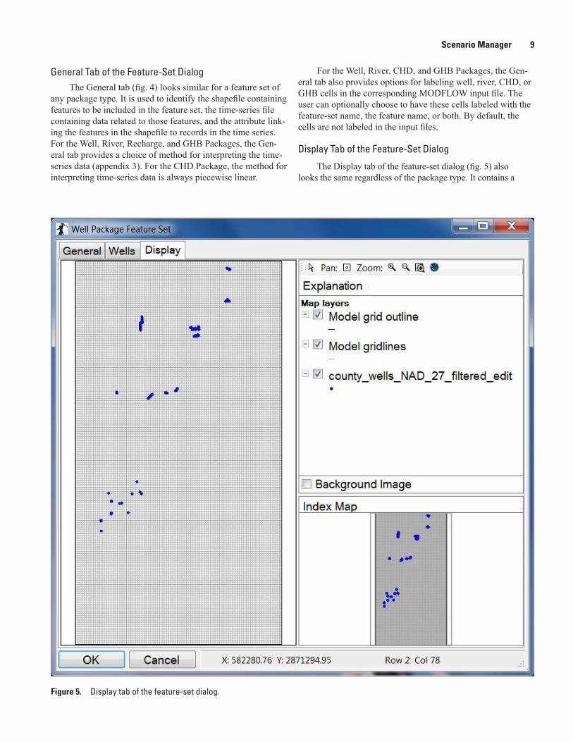
Display Tab of the Feature-Set Dialog
The Display tab of the feature-set dialog (fig. 5) also looks the same regardless of the package type. It contains a
Figure 5. Display tab of the feature-set dialog.

10 Two Graphical User Interfaces for Managing and Analyzing MODFLOW Groundwater-Model Scenarios
main image on the left side and an index map in the lower right corner. A list of viewable map layers is in the Explanation in the upper right corner. The Display tab is useful for ensuring that the shapefile contains the features that the user would like to include in the feature set. Checkboxes in the list of map layers allow the user to show or hide the model-grid outline, lines delimiting each model cell, and the features contained in the shapefile associated with the feature set. If the Scenario Man-ager project includes a georeferenced background image, the “Background image” checkbox can be used to turn the image on and off. Pan and zoom controls, located above the Explana-tion, can be used to manipulate the main image (table 1). The index map always displays the full extent of the visible images. When the main image is zoomed in, the index map also shows a rectangle corresponding to the main image area. Clicking on the index map recenters the main image on the point clicked.
Wells Tab of the Feature-Set Dialog
For each well to be simulated by the Well Package, a layer index needs to be specified. The Wells tab (fig. 6) pro-vides three options for assigning layer index:
• Assign all wells in the feature set to a specified layer;
• Assign layer according to the value of a specified attribute in the shapefile attribute table; or
• Let Scenario Manager assign layer index by compar-ing cell tops and bottoms to well open- or screened-interval top and bottom elevations stored as attributes in the shapefile attribute table.
The first two options are straightforward and result in at most one well cell per point feature in the shapefile. When the third option is used, Scenario Manager will generate a well cell for any model cell for which the cell top is above the interval bottom elevation and the cell bottom is below the interval top elevation. When more than one model cell satisfies these criteria, multiple well cells are generated. In this situation, the withdrawal or injection rate for the well is apportioned among the well cells according to the length of the open or screened interval in each cell, relative to the total length of open or screened interval in all well cells. “Quasi-3D” confining layers (Harbaugh, 2005) are ignored in the apportioning procedure.
Table 1. Pan and zoom icons and functions of the Display tab of the feature-set dialog.
Button icon Function
Deactivate pan and zoom functions.
Click main image to recenter image at pointer location.
Click main image to enlarge image by fixed amount, centered at pointer location.
Click main image to reduce image scale by fixed amount, centered at pointer location.
Scale main image to fit model grid.
Scale main image to fit full extent of visible images.

Scenario Manager 11
Figure 6. Wells tab of the feature-set dialog.
12 Two Graphical User Interfaces for Managing and Analyzing MODFLOW Groundwater-Model Scenarios
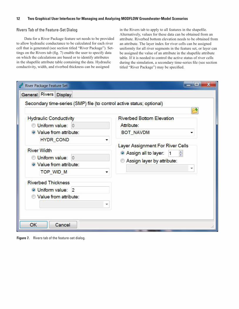
Rivers Tab of the Feature-Set Dialog
Data for a River Package feature set needs to be provided to allow hydraulic conductance to be calculated for each river cell that is generated (see section titled “River Package”). Set-tings on the Rivers tab (fig. 7) enable the user to specify data on which the calculations are based or to identify attributes in the shapefile attribute table containing the data. Hydraulic conductivity, width, and riverbed thickness can be assigned
Figure 7. Rivers tab of the feature-set dialog.
in the Rivers tab to apply to all features in the shapefile. Alternatively, values for these data can be obtained from an attribute. Riverbed bottom elevation needs to be obtained from an attribute. The layer index for river cells can be assigned uniformly for all river segments in the feature set, or layer can be assigned the value of an attribute in the shapefile attribute table. If it is needed to control the active status of river cells during the simulation, a secondary time-series file (see section titled “River Package”) may be specified.
Scenario Manager 13
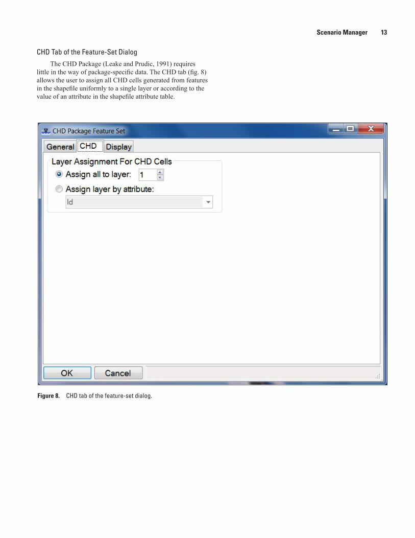
CHD Tab of the Feature-Set DialogThe CHD Package (Leake and Prudic, 1991) requires
little in the way of package-specific data. The CHD tab (fig. 8) allows the user to assign all CHD cells generated from features in the shapefile uniformly to a single layer or according to the value of an attribute in the shapefile attribute table.
Figure 8. CHD tab of the feature-set dialog.
14 Two Graphical User Interfaces for Managing and Analyzing MODFLOW Groundwater-Model Scenarios
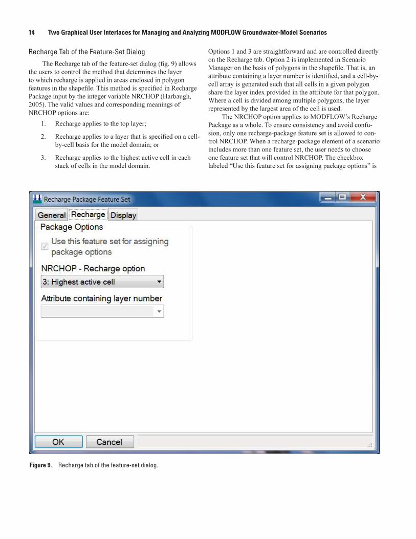
Recharge Tab of the Feature-Set DialogThe Recharge tab of the feature-set dialog (fig. 9) allows
the users to control the method that determines the layer to which recharge is applied in areas enclosed in polygon features in the shapefile. This method is specified in Recharge Package input by the integer variable NRCHOP (Harbaugh, 2005). The valid values and corresponding meanings of NRCHOP options are:
1. Recharge applies to the top layer;
2. Recharge applies to a layer that is specified on a cell-by-cell basis for the model domain; or
3. Recharge applies to the highest active cell in each stack of cells in the model domain.
Options 1 and 3 are straightforward and are controlled directly on the Recharge tab. Option 2 is implemented in Scenario Manager on the basis of polygons in the shapefile. That is, an attribute containing a layer number is identified, and a cell-by-cell array is generated such that all cells in a given polygon share the layer index provided in the attribute for that polygon. Where a cell is divided among multiple polygons, the layer represented by the largest area of the cell is used.
The NRCHOP option applies to MODFLOW’s Recharge Package as a whole. To ensure consistency and avoid confu-sion, only one recharge-package feature set is allowed to con-trol NRCHOP. When a recharge-package element of a scenario includes more than one feature set, the user needs to choose one feature set that will control NRCHOP. The checkbox labeled “Use this feature set for assigning package options” is
Figure 9. Recharge tab of the feature-set dialog.

Scenario Manager 15
used to make the choice. By default, the first feature set added to a recharge-package element will have the box checked, and feature sets added later will have the box unchecked. Checking the box for one feature set will automatically uncheck the box for other feature sets.
GHB Tab of the Feature-Set DialogAs described in the “GHB Package” section, leakance
may be assigned as a uniform value that applies to all poly-gons in the shapefile associated with a GHB-package feature set. Alternatively, leakance may be provided on a polygon-by-polygon basis as an attribute in the shapefile attribute table. The GHB tab (fig. 10) allows the user to make this choice. The tab also allows the user to assign all GHB cells generated by the feature set to a selected layer or choose an attribute containing layer number for each polygon. If needed to control the active status of GHB cells, a secondary time-series file (see “GHB Package” section) may be specified.
Manipulating Scenario Elements
To facilitate construction of scenarios that share some scenario elements with a previously constructed scenario, Scenario Manager provides capabilities to cut, copy, paste, and move packages and feature sets displayed in the scenario design panel or to duplicate an entire scenario. Any scenario, package, or feature set may be deleted. These capabilities are described in the following paragraphs.
To duplicate a scenario, first select the scenario by clicking on it. A duplicate of the selected scenario can be made either by using the menu item Edit | Duplicate Scenario or by right-clicking on the scenario and choosing Duplicate Scenario from the pop-up menu. A default scenario ID will be provided.
To delete any type of scenario element, select it and press the Delete key. Alternatively, a scenario element can be deleted by selecting it and using the menu item Edit | Delete. An element also can be deleted by right-clicking it and select-ing Delete. When an element is deleted, it cannot be pasted.
Figure 10. GHB tab of the feature-set dialog.

16 Two Graphical User Interfaces for Managing and Analyzing MODFLOW Groundwater-Model Scenarios
To cut a package or feature set, either select it and use the menu item Edit | Cut or right-click it and select Cut from the pop-up menu. A package that is cut will be removed from its scenario and can be pasted into another scenario that lacks a package of the type that was cut. A feature set that is cut will be removed from its package and can be pasted into a package of the same type in another scenario.
To copy a package or feature set, either select it and use the menu item Edit | Copy or right-click it and select Copy from the pop-up menu. An element that has been copied can be pasted as described in the next paragraph.
To paste a package or feature set that has been cut or copied, either right-click the element to which the cut or cop-ied element is to be pasted and select Paste from the pop-up menu or select the target element to which the element is to be pasted and use the menu item Edit | Paste. A package that is cut or copied can be pasted only into a target scenario that lacks a package of the type cut or copied. A feature set that is cut or copied can be pasted only into a target package of the same type in another scenario.
To move a package or feature set, the user can combine “cut” and “paste” procedures. Alternatively, a package or feature set can be moved in one operation by using only the mouse. To move a package or feature set by using the mouse, use the “drag-and-drop” operation: depress the left mouse but-ton on the element to be moved, drag the mouse to the target element, and release the mouse button. A drag-and-drop opera-tion is equivalent to a cut followed by a paste. The restrictions described previously for pasting also apply when using a drag-and-drop operation.
Scenario Manager also supports “undo” and “redo” operations. To undo a change, use the <Ctrl>-Z key combina-tion or the menu item Edit | Undo. Repetitions of <Ctrl>-Z or Edit | Undo will undo earlier changes, back to the most recent file save. The <Ctrl>-Y key combination or the menu item Edit | Redo will “redo” a change that has been undone.
Running Scenario SimulationsWhen one or more scenarios containing packages and
feature sets have been set up as desired, Scenario Manager can be used to export a set of files needed to run a scenario simulation and then, optionally, start the simulation. When a scenario is exported, a batch file that can be used separately to run the scenario simulation is written to the folder containing the master name file. To export only the model-input files and generate the batch file for a single scenario, select the scenario and then use the menu item Export | Export Scenario. After exporting a scenario, the scenario simulation can be started by running the batch file either in an MS-DOS window or by opening it in Windows Explorer.
To export the model-input files, generate the batch file, and start a scenario simulation, select the scenario and use the menu item Export | Export Scenario and Run Simulation. When this menu item is used, Scenario Manager invokes the batch file after preparing the model-input files.
In some situations, a user may find it convenient to export and run all scenarios in a Scenario Manager project. For example, if the master name file is edited to add a pack-age not controlled by Scenario Manager, a user may want to export and rerun all scenarios. For convenience, all scenarios in a Scenario Manager project can be exported and run in one step. To do this, use the menu item Export | Export and Run All Scenarios. If the computer running Scenario Manager has multiple processors or processor cores, Scenario Manager can invoke simultaneous model runs to take advantage of the pro-cessing power of the computer. Each time Scenario Manager starts, it detects the number of processor cores in the computer. By default the Export and Run All Scenarios procedure will invoke a number of simultaneous model runs up to the number of processor cores. The user can limit the number of simul-taneous model runs that will be made by Scenario Manager. To adjust this limit, before invoking Export and Run All Scenarios, open the Scenario Manager Project Settings dialog by using the menu item Project | Settings and set “Maximum Number of Simultaneous Scenario Runs” as desired. Note that the “Maximum Number of Simultaneous Scenario Runs” set-ting is saved not in the Scenario Manager project file but in the Scenario Manager user-settings file.
Guidelines for Providers of Base ModelsTo facilitate successful and appropriate use of Scenario
Manager, providers of base models are encouraged to provide models, data, and accompanying documentation according to the following guidelines:
• Identify the time and length units used in the model and assign ITMUNI and LENUNI of the MODFLOW discretization file accordingly. The user needs to be able to ensure that units of items in shapefile attributes and time-series files that are used to generate model input are consistent with the model units.
• Include at least one DATA(BINARY) file for cell-by-cell budget data in the name file. Set the appropriate variable in flow-package (Block-Centered Flow [BCF; Harbaugh, 2005], Layer Property Flow [LPF; Har-baugh, 2005], Hydrologic-Unit Flow [HUF; Ander-man and Hill, 2000], or Upstream Weighting [UPW; Niswonger and others, 2011]) input to the unit number associated with this file. Specify “REPLACE” as the “Fstatus” option (Harbaugh, 2005) for each file intended for output of cell-by-cell budget data.
• Include a DATA(BINARY) file for calculated heads in the name file. Specify “REPLACE” as the “Fstatus” option (Harbaugh, 2005).
• Provide an Output Control file that is set up to save budget and head data to binary files. Ideally, output is saved at every time step. Use of Scenario Analyzer with models generated by Scenario Manager depends on data in the binary files generated by MODFLOW.

Scenario Analyzer 17
Providers of base models are encouraged to specify the “COMPACT BUDGET” option to minimize file size and to provide maximum flexibility with respect to the use of Scenario Analyzer.
• Provide package-by-package guidance for the user regarding appropriate ranges of values for model inputs user will be making. If the user will be using Scenario Manager to generate input for the RIV Pack-age, provide guidance related to appropriate lengths for river segments, and potential error related to assignment of stage by segment.
• Identify the values of HNOFLO, HDRY, and CINACT that are used in model input, as described in the “Scenario Analyzer Settings” section.
• For any DATA or DATA(BINARY) file used as model input in the name file, specify “OLD” as the “Fstatus” option (Harbaugh, 2005). Use of the “OLD” option enables multiple scenarios to be run simultaneously.
• Identify the projected coordinate system used in con-structing the model grid.
• Provide example shapefiles and time-series data files suitable for generating scenarios that may be of inter-est to the client. At a minimum, these would include shapefiles and time-series data files that can be used to regenerate the original input files for the packages supported by Scenario Manager.
Scenario AnalyzerScenario Analyzer is a GUI for making maps, charts,
and tables illustrating data extracted from files generated by MODFLOW-based groundwater modeling programs and other data sources (appendix 3). Results can be viewed onscreen and exported to a PDF file. An exported PDF file includes meta-data documenting the data source(s) for the maps and charts. Scenario Analyzer is well-suited as a postprocessor for sce-nario simulations generated by Scenario Manager. However, Scenario Analyzer is not limited to this use—it can be used to analyze output from any compatible, MODFLOW-based modeling program.
Scenario Analyzer has been tested with MOD-FLOW–2005 (Harbaugh, 2005) and SEAWAT (version 4) (Langevin and others, 2008). Scenario Analyzer also can be used with any program that writes unstructured binary data in a form generated by MODFLOW–2005 or SEAWAT (version 4). Scenario Analyzer can extract and use hydraulic head, draw-down, and cell-by-cell budget data from binary files generated by MODFLOW–2005, SEAWAT ver. 4, MODFLOW–2000 (Harbaugh and others, 2000) (version 1.2 or later), MOD-FLOW–LGR (Mehl and Hill, 2005), MODFLOW–NWT (Nis-wonger and others, 2011) and various other MODFLOW-based
groundwater-modeling programs. It also can extract and use concentration data from binary files generated by SEAWAT ver. 4 and MT3DMS (Zheng and Wang, 1999).
A Scenario Analyzer project includes information required to generate one or more maps, charts, and tables. This information is stored in a Scenario Analyzer project file, which is identified by the “sa” extension.
Maps, Charts, and Tables
Each map, chart, or table is one display element of a Scenario Analyzer project. Maps generated by Scenario Analyzer show geographic distribution of some quantity or quantities extracted or derived from model output for the model domain. When a Scenario Analyzer project includes maps, a model-grid shapefile (appendix 3) needs to be speci-fied to georeference the map data to a projected coordinate system. Geographic distribution of a quantity can be depicted either by contours (lines of equal value) or by color fill (grada-tions of color). The charts and tables supported by Scenario Analyzer depict or list one or more time-dependent values of some quantities. In all cases, each quantity is defined as a data series. Each type of display element can include one or more data series. The two types of data series that are supported in Scenario Analyzer are described in the next section.
Data Series and Data Sets
In Scenario Analyzer, a data series consists of a data set and supplementary information. The data set contains the actual data; the supplementary information may specify, for example, display colors or contour intervals. A data set can be either a 2-dimensional (2D) array of values referenced by row and column indices to the model grid or a time series of numeric data. Each display-element type can only accommo-date data series of a given type. Each data series identifies a “data category” for the data that is contained in the data set.
Maps require data series that contain a 2D array. The array of values can be extracted from model output or can be the result of calculations based on other 2D array data series.
Charts and tables require data series that contain a time series of numeric values. Time-series data can be read from a file (appendix 3), extracted from output of a transient model run, or calculated from other time series. A time series of data can be extracted from model output for an individual model cell or for a user-defined group of model cells.
MODFLOW and related programs can generate binary files of two types, both of which can be used by Scenario Analyzer as data sources. The first type is designed to hold values of hydraulic head or drawdown. This type is also used by SEAWAT (version 4) and MT3DMS to store values of solute concentration. The second type is designed to hold cell-by-cell water-budget data associated with individual packages that are used in a simulation. A data series of either type can be populated with data extracted from either type of binary
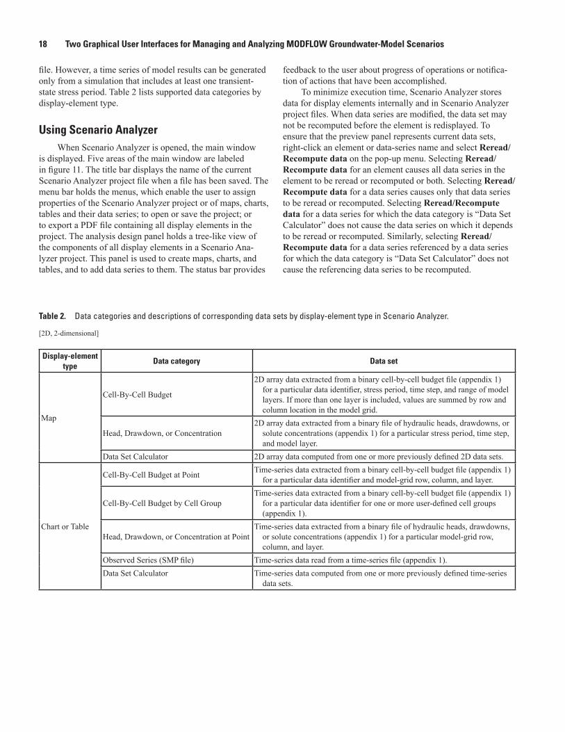
18 Two Graphical User Interfaces for Managing and Analyzing MODFLOW Groundwater-Model Scenarios
file. However, a time series of model results can be generated only from a simulation that includes at least one transient-state stress period. Table 2 lists supported data categories by display-element type.
Using Scenario AnalyzerWhen Scenario Analyzer is opened, the main window
is displayed. Five areas of the main window are labeled in figure 11. The title bar displays the name of the current Scenario Analyzer project file when a file has been saved. The menu bar holds the menus, which enable the user to assign properties of the Scenario Analyzer project or of maps, charts, tables and their data series; to open or save the project; or to export a PDF file containing all display elements in the project. The analysis design panel holds a tree-like view of the components of all display elements in a Scenario Ana-lyzer project. This panel is used to create maps, charts, and tables, and to add data series to them. The status bar provides
Table 2. Data categories and descriptions of corresponding data sets by display-element type in Scenario Analyzer.
[2D, 2-dimensional]
Display-element type
Data category Data set
Map
Cell-By-Cell Budget
2D array data extracted from a binary cell-by-cell budget file (appendix 1) for a particular data identifier, stress period, time step, and range of model layers. If more than one layer is included, values are summed by row and column location in the model grid.
Head, Drawdown, or Concentration2D array data extracted from a binary file of hydraulic heads, drawdowns, or
solute concentrations (appendix 1) for a particular stress period, time step, and model layer.
Data Set Calculator 2D array data computed from one or more previously defined 2D data sets.
Chart or Table
Cell-By-Cell Budget at Point Time-series data extracted from a binary cell-by-cell budget file (appendix 1) for a particular data identifier and model-grid row, column, and layer.
Cell-By-Cell Budget by Cell GroupTime-series data extracted from a binary cell-by-cell budget file (appendix 1)
for a particular data identifier for one or more user-defined cell groups (appendix 1).
Head, Drawdown, or Concentration at PointTime-series data extracted from a binary file of hydraulic heads, drawdowns,
or solute concentrations (appendix 1) for a particular model-grid row, column, and layer.
Observed Series (SMP file) Time-series data read from a time-series file (appendix 1).Data Set Calculator Time-series data computed from one or more previously defined time-series
data sets.
feedback to the user about progress of operations or notifica-tion of actions that have been accomplished.
To minimize execution time, Scenario Analyzer stores data for display elements internally and in Scenario Analyzer project files. When data series are modified, the data set may not be recomputed before the element is redisplayed. To ensure that the preview panel represents current data sets, right-click an element or data-series name and select Reread/Recompute data on the pop-up menu. Selecting Reread/Recompute data for an element causes all data series in the element to be reread or recomputed or both. Selecting Reread/Recompute data for a data series causes only that data series to be reread or recomputed. Selecting Reread/Recompute data for a data series for which the data category is “Data Set Calculator” does not cause the data series on which it depends to be reread or recomputed. Similarly, selecting Reread/Recompute data for a data series referenced by a data series for which the data category is “Data Set Calculator” does not cause the referencing data series to be recomputed.

Scenario Analyzer 19
Figure 11. Scenario Analyzer main window, with areas labeled.

20 Two Graphical User Interfaces for Managing and Analyzing MODFLOW Groundwater-Model Scenarios
Figure 12. Scenario Analyzer project settings dialog.
Scenario Analyzer Settings
Settings that apply to the Scenario Analyzer project as a whole or are shared among display elements in a project are accessed on the General tab of the “Scenario Analyzer Project Settings” dialog (fig. 12). The Scenario Analyzer Project Settings dialog can be accessed either with the Project | Settings menu item or by right-clicking in a blank area of the analysis design panel and selecting Project Set-tings on the pop-up menu. When the project is exported to a PDF file, the report name and author (“Name” and “Author” fields, respectively) are written to the first page of that file. When the project contains one or more maps, the user needs to provide the name of a polygon shapefile of the model grid (appendix 3) in the field labeled “Model-Grid Shapefile.” A georeferenced image file (appendix 3) can be used as a background image for maps; if maps do not need a back-ground image, the “Georeferenced Background Image File” field can be left blank. HNOFLO, HDRY, and CINACT are values that are user-specified in input to MODFLOW and related programs. These values are written by MOD-FLOW or a related program to 2D arrays of hydraulic head,
drawdown, or solute concentration for any cell location where a simulated value is not available. To ensure that these values are correctly treated as “no-data” values, the Scenario Analyzer user needs to enter the values provided to MOD-FLOW or related program in the corresponding fields of the Scenario Analyzer Project Settings dialog. HNOFLO is read by MODFLOW and related programs in the Basic Package input file (Harbaugh, 2005). HDRY is read by the LPF, BCF (Harbaugh, 2005), HUF (Anderman and Hill, 2000), or UPW (Niswonger and others, 2011) Package in the correspond-ing input file. CINACT is read by MT3DMS (Zheng and Wang, 1999) in the Basic Transport (BTN) Package input file when SEAWAT (version 4) (Langevin and others, 2008) or MT3DMS is used. The Elements and Map Extents tabs are discussed in the “Ordering Report Elements and Managing Map Extents” section.
Making a MapBefore any map can be constructed, the model-grid
geometry and dimensions need to be defined by supplying the name of a polygon shapefile of the model grid (appendix 3)

Scenario Analyzer 21
in the Scenario Analyzer Project Settings dialog (see previous section). If the user attempts to make a map without having defined the model grid, a warning is issued.
A new, empty map can be added to the analysis design panel in either of two ways: (1) by right-clicking in a blank area of the analysis design panel and selecting Add New Map on the pop-up menu, or (2) by using the Edit | Add New Map menu item. When a new map is added by either method, the Map Designer dialog appears (fig. 13). At this time the map can be given a name by entering text in the Name field. If no name is entered, the name will default to “Unnamed Map.” The empty map can be saved by clicking OK. The Map Designer dialog can be reopened from the main window either by right-clicking the map node and selecting Proper-ties on the pop-up menu, by double-clicking the map node, or by selecting the map node and selecting the menu item Edit | Element Properties. After the Map Designer dialog has been dismissed by clicking OK, a map node (table 3) will be added in the analysis design panel of the main window.
For maps, each data series generates a map layer. Each map layer is either a contour layer or a color-fill layer. Any
number of map layers can be added to a map, but if a map contains multiple color-fill layers that overlap, only the upper-most layer will be visible in the overlap area. To add a map
Figure 13. Map Designer dialog, with map preview panel labeled.
Table 3. Icons of the analysis design panel and their significance.
Icon Significance
Identifies a map node
Identifies a chart node
Identifies a table node
Data are being processed
Data have been successfully processed
Warning
Error

22 Two Graphical User Interfaces for Managing and Analyzing MODFLOW Groundwater-Model Scenarios
layer to a map, right-click the map node and select either Add New Contour Layer or Add New Color-Fill Layer. Alter-natively, select the map node, open the Edit menu, and select either Add New Contour Layer or Add New Color-Fill Layer. In either case, a “Data Series” dialog will open, with fields appropriate for either a contour layer or a color-fill layer. Data for map layers can be extracted from a MODFLOW-generated file of hydraulic heads or drawdowns or a cell-by-cell budget file, or from an MT3DMS- or SEAWAT-generated file of solute concentrations (appendix 3).
The dialogs for editing contour map layers and color-fill map layers (figs. 14–16) provide controls for defining data sets in the box labeled “Data Set.” The set of controls contained in the “Data Set” box changes, depending on the selected data category. For each map layer, the user is given the option to make the layer visible or not. This flexibility is useful in designing and constructing an uncluttered map.
If the location of a georeferenced background image file has been entered on the “Scenario Analyzer Project Settings” dialog (see section titled “Scenario Analyzer Settings”), the image can be displayed as a background image for any map. The background image can be lightened or darkened by
adjusting the “Brightness” control on the Layout tab of the Map Designer dialog (fig. 13).
Data Sources for Map LayersEach map layer is based on a particular data set. The data
set may be extracted from one of the MODFLOW-generated binary files (appendix 3), or it may be calculated from one or more other, previously defined, data series. Data-series dialogs (figs. 14–16) contain a drop-down list labeled “Data Category,” which allows the user to specify the category of data in the data set included in the data series. Table 2 lists supported data cat-egories and corresponding data sets for maps, charts, and tables.
Contour Map LayersIf a contour map layer is added, a dialog titled “Data
Series for a Contour Map Layer” will open (fig. 14). A user-selected name can be provided in the Name field; if it is left blank, the name will default to the text that appears in the Data Category field.
The Data Category field is a drop-down list from which the user can select one of the options listed for the “Map”
Figure 14. Data-series dialog for a contour map layer based on data from a cell-by-cell budget file.

Scenario Analyzer 23
element type in table 2. When this selection changes, the fields in the “Data Set” panel on the right side of the dialog are reconfigured to enable the user to provide information relevant to the selected data category.
If “Cell-By-Cell Budget” is selected and “Equal Inter-val” is selected in the “Contour Interval” box, the dialog will look like figure 14. In this configuration, the user can browse to find a cell-by-cell budget file (appendix 3) and select the data set to be used. If a data set for the desired data identifier, stress period, and time step is known to be present in the file, the data identifier, stress period, and time step can be speci-fied using the “Data Identifier” drop-down list and “Stress Period” and “Time Step” fields, respectively. If not, the “View Available Data Sets” button can be used to open a dialog that allows the user to view the data sets contained in the selected cell-by-cell budget file and select the desired data set. The model layer(s) of interest are selected using the “Start Layer” and “End Layer” controls. If more than one layer is selected, values from multiple layers are summed for each row and column location.
If “Head, Drawdown, or Concentration” is selected, the dialog will look like figure 15. In this configuration, the user can browse to find a binary file containing values of hydraulic head, drawdown, or solute concentration and select the layer, stress period, and time step of the data set to be used. If the selected data file contains both hydraulic heads and draw-downs, the “Data Identifier” drop-down list provides a choice between the two.
The “Line Series Color” and “Contour Interval” boxes allow the user to control contour color and the contours that are drawn. “Automatic” is the default contour-interval method; it produces contours without further input from the user. When “Equal Interval” is selected, the user can specify numeric values for the starting contour and the contour interval. When “List of Values” is selected, a text box is provided where the user can enter a comma-separated list of numeric values indicating the contours that should be drawn.
Data extracted from a cell-by-cell budget file (or calcu-lated from other data series for which the data are extracted from a cell-by-cell budget file) are flow values, which have
Figure 15. Data-series dialog for a contour map layer based on data from a head, drawdown, or concentration file.

24 Two Graphical User Interfaces for Managing and Analyzing MODFLOW Groundwater-Model Scenarios
units of L3/T. When these data are used to generate a map layer, converting the flow values to flux values (units: L/T) by dividing by model-cell area may result in a more mean-ingful and informative way to display the data, particularly when cell dimensions are not uniform. The checkbox labeled “For display, convert flow (L**3/T) values to flux (L/T) values” (fig. 14) provides the user with the option to make this conversion.
Color-Fill Map LayersIf a color-fill map layer is added, a dialog titled “Data
Series for a Color-Fill Map Layer” will open. When this dialog first opens, the data category defaults to “Cell-By-Cell Budget,” and the “Data Set” box is like that shown in figure 14. If the data category is changed to “Data Set Calculator,” the “Data Set” box configuration changes to that shown in figure 16. Appendix 2 explains the use of the Data Set Calculator.
Defining a data set for a color-fill map layer is as described for a contour-map layer in the preceding section. Symbology for a color-fill map layer is controlled by a color ramp, where each model-grid cell is filled with a color on a gradated scale between the smallest and largest numeric values in a 2D array. The end members of the color ramp can be set by using the buttons on either end of the color-ramp represen-tation in the “Color Ramp” box (fig. 16). The button on the left side of the color ramp controls the color used for the smallest
value, and the button on the right side of the color ramp controls the color used for the largest value.
Map ExtentsEach map represents a well-defined rectangular area in
the projected coordinate system used for the map layers. In Scenario Analyzer, the term “extent” is used to refer to the set of coordinates defining the north, south, west, and east limits of a rectangle that can be used as the map limits. Each extent in a Scenario Analyzer project has a unique name. When a model-grid shapefile (appendix 3) is imported, an extent named “model grid” is created. After one or more map layers have been added to a map, the Map Designer dialog can be used to create new extents. A new extent can be created graphically in the map preview panel of the Layout tab of the Map Designer dialog (fig. 17) by using the mouse; depress the left mouse button and drag to define opposing corners of a rectangle. When a rectangle has been drawn and the mouse button is released, the “Save Extent” button is enabled. Click-ing the “Save Extent” button opens a small dialog which can be used to provide a name for the extent and to manually adjust the extent coordinates. Alternatively, a new extent can be defined on the Extent tab of the Map Designer (fig. 18) by providing an extent name and coordinate values. The Extent tab can be used to select a previously defined extent or to edit coordinates of existing extents.
Figure 16. Data-series dialog for a color-fill map layer based on a calculated data set.
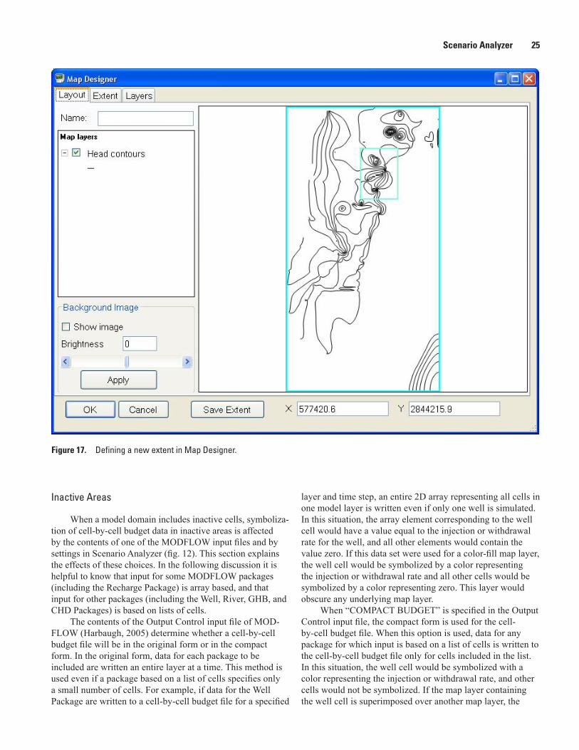
Scenario Analyzer 25
Inactive Areas
When a model domain includes inactive cells, symboliza-tion of cell-by-cell budget data in inactive areas is affected by the contents of one of the MODFLOW input files and by settings in Scenario Analyzer (fig. 12). This section explains the effects of these choices. In the following discussion it is helpful to know that input for some MODFLOW packages (including the Recharge Package) is array based, and that input for other packages (including the Well, River, GHB, and CHD Packages) is based on lists of cells.
The contents of the Output Control input file of MOD-FLOW (Harbaugh, 2005) determine whether a cell-by-cell budget file will be in the original form or in the compact form. In the original form, data for each package to be included are written an entire layer at a time. This method is used even if a package based on a list of cells specifies only a small number of cells. For example, if data for the Well Package are written to a cell-by-cell budget file for a specified
layer and time step, an entire 2D array representing all cells in one model layer is written even if only one well is simulated. In this situation, the array element corresponding to the well cell would have a value equal to the injection or withdrawal rate for the well, and all other elements would contain the value zero. If this data set were used for a color-fill map layer, the well cell would be symbolized by a color representing the injection or withdrawal rate and all other cells would be symbolized by a color representing zero. This layer would obscure any underlying map layer.
When “COMPACT BUDGET” is specified in the Output Control input file, the compact form is used for the cell-by-cell budget file. When this option is used, data for any package for which input is based on a list of cells is written to the cell-by-cell budget file only for cells included in the list. In this situation, the well cell would be symbolized with a color representing the injection or withdrawal rate, and other cells would not be symbolized. If the map layer containing the well cell is superimposed over another map layer, the
Figure 17. Defining a new extent in Map Designer.

26 Two Graphical User Interfaces for Managing and Analyzing MODFLOW Groundwater-Model Scenarios
Figure 18. Extent tab of Map Designer.
symbolization of the well cell would obscure information in the underlying map layer at that cell location, but informa-tion in other areas would not be obscured. For this reason, the “COMPACT BUDGET” option needs to be used when maps are to include color-fill map layers showing cell-by-cell bud-get contributions from multiple packages. Providers of base models are encouraged to specify the “COMPACT BUD-GET” option to minimize file size and to provide maximum flexibility with respect to map design.
The IBOUND arrays of MODFLOW input (Harbaugh, 2005) specify active and inactive cells for each model layer. When cell-by-cell budget data for a package for which input is array based is used in generating a map layer (or for any package when the cell-by-cell budget file is in the original form), the user can choose whether areas of inactive cells are to be symbolized or left blank. For example, if a map layer is to show recharge rates over the domain of a model having an irregular active area, the cell-by-cell budget file generated by the model would contain values of zero for inactive cells. Controls on the “Inactive Areas” tab of the “Scenario Analyzer
Project Settings” window allow the user to specify whether these areas are to be symbolized by a value of zero or are to be left blank. The settings on the “Inactive Areas” tab apply to all map layers in all maps included in a Scenario Analyzer proj-ect. To allow values of zero to be symbolized (for example, on color-fill map layers), select the “Leave as is” option, which is the default. To use inactive cells as specified in the IBOUND arrays to define areas that are to be left blank, select one of the following three options, which are self-explanatory:
• Blank by specified IBOUND layer,
• Blank where IBOUND inactive in any layer, or
• Blank where IBOUND inactive in all layersWhen one of these three options is selected, the user
needs to provide the path name of a MODFLOW name file that contains an entry for the Basic Package input file (Har-baugh, 2005) used for the model of interest. If the model was generated using Scenario Manager, this file generally would be the master MODFLOW name file.

Scenario Analyzer 27
Ordering Map LayersMap layers are drawn in order from the bottom to the top
of the list that is displayed on the Layers tab of Map Designer (fig. 19). Draw order for map layers is important because lay-ers drawn earlier can be partly or entirely hidden by a layer that is drawn later. A layer can be selected in the Layers tab by clicking on the map-layer name; the selected layer will be highlighted in blue. When a layer is selected, the arrow but-tons on the right side of the Layers tab can be used to move the selected layer up or down in the list. The selected layer also can be deleted by using the “X” button.
Making a ChartIn Scenario Analyzer, a chart provides a graphic represen-
tation of one or more time-series data sets. Data sets may con-tain values extracted from output generated by a transient-state MODFLOW model or read from a time-series data file (appen-dix 3). Data sets also can be generated by the Data Set Calcula-tor (appendix 2). To add a chart to a Scenario Analyzer project, right-click in the analysis design panel (fig. 11) and select Add New Chart. Alternatively, a chart can be added by using menu item Edit | Add New Chart. A dialog titled “Report Chart” will open (fig. 20). A name for the chart can be provided; if the Name field is left blank, the chart name defaults to “Unnamed Chart.” Clicking OK saves the new chart.
A data series can be added to a chart by right-clicking on the chart element in the analysis design panel of the main Scenario Analyzer window (fig. 11) and selecting Add New Data Series. When a new data series is added to a chart, a dia-log titled “Data Series for a Chart” opens (fig. 21). A name for the chart can be provided. A data category for the data series needs to be selected in the drop-down list; options are listed in table 2. After the data category has been selected, informa-tion to define the data set can be entered in the “Data Set” box. Time-series data to be plotted on a chart can be extracted from binary MODFLOW output files or read from time-series data files (appendix 3). Data extracted from MODFLOW output files can be for a specific cell in the model grid, or for a cell group (table 2, appendix 3). As for map layers, the controls displayed in the “Data Set” box are reconfigured when the data category is selected. Line and point-symbol colors can be assigned for each data series as desired (fig. 21).
Axes limits for a chart can be set on the Domain/Range tab (not shown) of the Report Chart dialog. The “Data Series” tab (not shown) can be used to modify the draw order for a chart’s data series or to delete data series.
Making a TableThe process of creating a table in Scenario Analyzer
is similar to that described in the preceding section; the
Figure 19. Layers tab of Map Designer.

28 Two Graphical User Interfaces for Managing and Analyzing MODFLOW Groundwater-Model Scenarios
Figure 20. Report chart dialog.
Figure 21. Data-series dialog for a chart.

Scenario Analyzer 29
differences are described here. To add a table, right-click in the analysis design panel (fig. 11) and select Add New Table, or use menu item Edit | Add New Table. When a table is added, a dialog titled “Report Table” will open (fig. 22). In a table, the first column always contains a date; to also include the time in the first column, check the box labeled “Include Time in Table.” The starting and ending date for all rows of the table can be set on the “Range” tab (not shown).
The number of rows in a table and the date and time represented by each row are determined by the first data series included in the table. If the first data series is for data extracted from a binary MODFLOW output file (appendix 3), a row is defined for each time step for which the file contains data for the selected data identifier. If the first data series reads data from a time-series data file (appendix 3), a row is defined for each time represented in the time series. The “Columns” tab of the Report Table dialog can be used to reorder the data series included in a table, thereby controlling the rows and corre-sponding times included in the table.
There is no requirement that all data series in a table include data for times matching those included in the time series of the first data series in a table. When a value is needed for a time not represented in a time-series data set, a value is linearly interpolated from values for adjacent times. If a value cannot be interpolated because the data series lacks data for a time preceding or following the time of interest, “NaN” is written in the table cell, where NaN stands for “not a number.”
Table data can be exported to a comma-separated value (CSV) file to facilitate further processing. To export table data, right-click on a table element in the analysis design panel of the main Scenario Analyzer window and select Export CSV
File on the pop-up menu. A dialog will ask for the name of a file to which the data are to be saved. A CSV file can be opened by most spreadsheet applications.
Ordering Report Elements and Managing Map Extents
Before exporting a report, the user may want to change the order in which elements appear in the report. Element order is controlled in the “Elements” tab (not shown) of the Scenario Analyzer Project Settings dialog (see section titled “Scenario Analyzer Settings” and fig. 12).
When a map extent is defined for one map, it becomes available for use in all maps in a Scenario Analyzer project. As extents are added, the user may find that a project con-tains more extents than are required. Unneeded extents can be removed from a Scenario Analyzer project using the “Map Extents” tab of the “Scenario Analyzer Project Settings” dialog. To remove an extent, select it by clicking on the extent name and then click the “X” button. Scenario Analyzer will not allow the “model grid” extent or any extent that is in use to be removed. To select multiple map extents for deletion, hold down the <Ctrl> key while clicking on the desired extents. To select a range of map extents, click on the first map extent in the range then hold down the <Shift> key and click on the last extent in the range.
Exporting a ReportWhen a Scenario Analyzer project contains elements con-
figured and ordered as desired, a PDF file containing all element
Figure 22. Report Table dialog.

30 Two Graphical User Interfaces for Managing and Analyzing MODFLOW Groundwater-Model Scenarios
and supporting documentation can be exported. Before doing so, the user may want to provide a report name and author in the Scenario Analyzer Project Settings dialog (fig. 12).
To export the project to a PDF file, use the menu item File | Export to PDF. A dialog will ask for a location and file name for the PDF file. After providing those, click Save to export the report.
The exported report will have a title page, showing the author and date, and one or more pages for each display ele-ment. Metadata describing the source of data for each visible data series of each map or chart will be included following the map or chart. If needed, the metadata descriptions continue on following page or pages.
AcknowledgmentsThe author expresses gratitude to the following develop-
ers and providers of libraries of software. Without the avail-ability of these libraries, timely development of the applica-tions described in this report would not have been possible.
• David Pollock (2012), whose Puma Framework, distrib-uted with MODPATH Output Examiner (http://water.usgs.gov/ogw/modpath/moe.html), was used extensively.
• FW-Tools (http://fwtools.maptools.org/)
• Geospatial Data Abstraction Library (http://www.gdal.org/)
• GeoAPI.NET (http://geoapi.codeplex.com/)
• Haru free PDF library (http://libharu.org/)
• NetTopologySuite (http://code.google.com/p/nettopologysuite/)
• SharpMap (http://sharpmap.codeplex.com/)
• SharpZip (http://www.icsharpcode.net/opensource/sharpziplib/)
• Software Productions, for Undo/Redo capabilities (no longer available online)
References Cited
Adobe Systems, Inc., 2013, About Adobe PDF: Adobe Sys-tems, Inc., available at http://www.adobe.com/products/acrobat/adobepdf.html. (Accessed May 10, 2013.)
Anderman, E.R., and Hill, M.C., 2000, MODFLOW-2000, the U.S. Geological Survey modular ground-water model—Documentation of the hydrogeologic-unit flow (HUF) pack-age: U.S. Geological Survey Open-File Report 00-342, 89 p. Available online at http://water.usgs.gov/nrp/gwsoftware/modflow2005/modflow2005.html.
Banta, E.R., 2000, MODFLOW-2000, the U.S. Geological Survey modular ground-water model—Documentation of packages for simulating evapotranspiration with a segmented function (ETS1) and drains with return flow (DRT1): U.S. Geological Survey Open-File Report 00–466, 127 p. Available online at http://pubs.er.usgs.gov/pubs/ofr/ofr00466.
Doherty, John, 2011, Groundwater data utilities, Part A—Overview: Corinda, Australia, Watermark Numerical Com-puting, 61 p. Available online at http://www.pesthomepage.org/Downloads.php/. (Accessed May 10, 2013.)
Environmental Systems Research Institute, Inc., 1998, ESRI shapefile technical description: Environmental Systems Research Institute, Inc., 28 p. Available online at http://www.esri.com/library/whitepapers/pdfs/shapefile.pdf. (Accessed September 16, 2011.)
Fenske, J.P., Leake, S.A., and Prudic, D.E., 1996, Documen-tation of a computer program (RES1) to simulate leakage from reservoirs using the modular finite-difference ground-water flow model (MODFLOW): U.S. Geological Survey Open–File Report 96–364, 51 p. Available online at http://pubs.er.usgs.gov/publication/ofr96364.
Halford, K.J., and Hanson, R.T., 2002, User guide for the drawdown-limited, Multi-Node Well (MNW) Package for the U.S. Geological Survey’s modular three-dimensional finite-difference ground-water flow model, versions MOD-FLOW–96 and MODFLOW–2000: U.S. Geological Survey Open–File Report 02–293, 33 p. Available online at http://water.usgs.gov/nrp/gwsoftware/modflow2000/MNW_text.pdf.
Harbaugh, A.W., 2005, MODFLOW–2005, the U.S. Geologi-cal Survey modular ground-water model—The ground-water flow process: U.S. Geological Survey Techniques and Methods, book 6, chap. A16, variously paginated. Avail-able online at http://pubs.usgs.gov/tm/2005/tm6A16/PDF/TM6A16.pdf.
Harbaugh, A.W., Banta, E.R., Hill, M.C., and McDonald, M.G., 2000, MODFLOW–2000, the U.S. Geological Sur-vey modular ground-water model—User guide to modu-larization concepts and the ground-water flow process: U.S. Geological Survey Open-File Report 00–92, 121 p. Available online at http://water.usgs.gov/nrp/gwsoftware/modflow2000/ofr00-92.pdf.
Hoffmann, Jörn, Leake, S.A., Galloway, D.L., and Wilson, A.M., 2003, MODFLOW–2000 ground-water model—User guide to the subsidence and aquifer-system compaction (SUB) package: U.S. Geological Survey Open–File Report 03–233, 44 p. Available online at http://pubs.er.usgs.gov/publication/ofr03233.
Hughes, J.D., Langevin, C.D., Chartier, K.L., and White, J.T., 2012, Documentation of the surface-water routing (SWR1) process for modeling surface-water flow with the U.S.

References Cited 31
Geological Survey modular ground-water model (MOD-FLOW-2005): U.S. Geological Survey Techniques and Methods, book 6, chap. A40 (Version 1.0), 113 p. Available online at http://pubs.usgs.gov/tm/6a40/.
Konikow, L.F., Hornberger, G.Z., Halford, K.J., and Hanson, R.T., 2009, Revised multi-node well (MNW2) package for MODFLOW ground-water flow model: U.S. Geological Survey Techniques and Methods, book 6, chap. A30, 67 p. Available online at http://pubs.usgs.gov/tm/tm6a30/.
Langevin, C.D., Thorne, D.T., Jr., Dausman, A.M., Sukop, M.C., and Guo, Weixing, 2008, SEAWAT Version 4—A computer program for simulation of multi-species solute and heat transport: U.S. Geological Survey Techniques and Methods, book 6, chap. A22, 39 p. Available online at http://pubs.usgs.gov/tm/tm6a22/.
Leake, S.A., and Galloway, D.L., 2007, MODFLOW ground-water model—User guide to the subsidence and aquifer-system compaction package (SUB–WT) for water-table aquifers: U.S. Geological Survey Techniques and Methods, book 6, chap. A23, 42 p. Available online at http://pubs.usgs.gov/tm/2007/06A23/pdf/TM6a23.pdf.
Leake, S.A., and Lilly, M.R., 1997, Documentation of a com-puter program (FHB1) for assignment of transient specified-flow and specified-head boundaries in applications of the modular finite-difference ground-water flow model (MOD-FLOW): U.S. Geological Survey Open-File Report 97–571, 50 p. Available online at http://pubs.er.usgs.gov/publication/ofr97571.
Leake, S.A., and Prudic, D.E., 1991, Documentation of a com-puter program to simulate aquifer-system compaction using the modular finite-difference ground-water flow model: U.S. Geological Survey Techniques of Water-Resources Investi-gations Report, book 6, chap. A2, 68 p. Available online at http://pubs.er.usgs.gov/publication/twri06A2.
Lohman, S.W., Bennett, R.R., Brown, R.H., Cooper, H.H., Jr., Drescher, W.J., Ferris, J.G., Johnson, A.I., McGuinness, C.L., Piper, A.M., Rorabaugh, M.I., Stallman, R.W., and Theis, C.V., 1972, Definitions of selected ground-water terms—Revisions and conceptual refinements: U.S. Geo-logical Survey Water-Supply Paper 1988, 21 p. Available online at http://pubs.er.usgs.gov/publication/wsp1988.
Mehl, S.W., and Hill, M.C., 2005, MODFLOW–2005, The U.S. Geological Survey modular ground-water model—Documentation of shared node local grid refinement (LGR) and the boundary flow and head (BFH) package: U.S. Geological Survey Techniques and Methods, book. 6, chap. A12, 68 p. Available online at http://water.usgs.gov/nrp/gwsoftware/modflow2005_lgr/mflgr.html.
Merritt, M.L., and Konikow, L.F., 2000, Documentation of a computer program to simulate lake-aquifer interaction using the MODFLOW ground-water flow model and the
MOC3D solute-transport model: U.S. Geological Survey Water-Resources Investigations Report 00-4167, 146 p. Available online at http://fl.water.usgs.gov/PDF_files/wri00_4167_merritt.pdf.
Niswonger, R.G., Panday, Sorab, and Ibaraki, Motomu, 2011, MODFLOW-NWT, A Newton formulation for MOD-FLOW–2005: U.S. Geological Survey Techniques and Methods, book 6, chap. A37, 44 p. Available online at http://pubs.usgs.gov/tm/tm6a37/.
Niswonger, R.G., and Prudic, D.E., 2006, Documentation of the streamflow-routing (SFR2) package to include unsatu-rated flow beneath streams—A modification to SFR1: U.S. Geological Survey Techniques and Methods, book 6, chap. A13, Version 1.10, April 2006, 48 p. Available online at http://pubs.usgs.gov/tm/2006/tm6A13/.
Niswonger, R.G., Prudic, D.E., and Regan, R.S., 2006, Docu-mentation of the unsaturated-zone flow (UZF1) package for modeling unsaturated flow between the land surface and the water table with MODFLOW–2005: U.S. Geological Survey Techniques and Methods, book 6, chap. A19, 62 p. Available online at http://pubs.usgs.gov/tm/2006/tm6a19/.
Pollock, D.W., 2012, User Guide for MODPATH version 6—A particle-tracking model for MODFLOW: U.S. Geo-logical Survey Techniques and Methods, book 6, chap. A41, 58 p. Available online at http://pubs.er.usgs.gov/publication/tm6A41.
Prudic, D.E., 1989, Documentation of a computer program to simulate stream-aquifer relations using a modular, finite-dif-ference, ground-water flow model: U.S. Geological Survey Open–File Report 88–729, 113 p. Available online at http://pubs.er.usgs.gov/publication/ofr88729.
Zheng, Chunmiao, and Wang, P.P., 1999, MT3DMS, A modu-lar three-dimensional multi-species transport model for sim-ulation of advection, dispersion and chemical reactions of contaminants in groundwater systems—Documentation and user’s guide: U.S. Army Engineer Research and Develop-ment Center Contract Report SERDP-99-1, Vicksburg, MS, 202 p. Available online at http://hydro.geo.ua.edu/mt3d/.
Publishing support provided by: Denver Publishing Service Center
For more information concerning this publication, contact:Director, USGS Colorado Water Science CenterBox 25046, Mail Stop 415Denver, CO 80225(303) 236-4882
Or visit the Colorado Water Science Center Web site at:http://co.water.usgs.gov/

Appendixes 1–3

Appendix 1 33
Appendix 1. GlossarySelected terms are briefly defined as used in this report.
Additional details for many of the terms related to ground-water, groundwater modeling, and MODFLOW can be found in Lohman and others (1972) or Harbaugh (2005).
Base model Model on which one or more model scenarios defined in a Scenario Manager project are based. Binary file A computer file used for storing data in a form not encoded as text.Data category In a data series defined in Scenario Analyzer, a setting that determines the way in which the data series obtains or generates data.Data series In Scenario Analyzer, a source of data for a map, chart, or table. The data series includes settings and informa-tion required to obtain or generate the data. Each map, chart, or table can include one or more data series.Data set In a data series defined in Scenario Analyzer, either a set of numeric values read from a file or an expression ref-erencing other data series, from which a set of numeric values is calculated.Dialog A window, other than the main windows of Scenario Manager and Scenario Analyzer, used for defining settings and data sources and for displaying information.Display element In Scenario Analyzer, either a map, a chart, or a table.Feature set In Scenario Manager, a collection of data sources and information that defines one or more hydrologi-cally significant features and related stresses to be simulated in a scenario. Each feature set is associated with a package and includes information needed to generate input for the package.Finite-difference grid A conceptual, two- or three-dimen-sional, rectilinear grid used to subdivide a model domain. The grid is subdivided into a specified number of layers in the ver-tical dimension and specified numbers of rows and columns in the horizontal dimensions.Hydraulic conductance A measure of the ease with which groundwater flows through a finite volume of porous medium of given cross-sectional area and length. Hydraulic conduc-tance is the product of hydraulic conductivity and cross-sectional area of flow divided by the length of the flow path. In MODFLOW, hydraulic conductance is defined for con-nections between adjacent model cells or between a model cell and an external, head-dependent source or sink of water. Units: L2T-1.Hydraulic conductivity The volume of water at the existing viscosity that will move through a porous medium in unit time under a unit hydraulic gradient through a unit area measured at right angles to the direction of flow. Units: LT-1.Hydraulic gradient The change in hydraulic head per unit of distance in a given direction. Units: LL-1 (dimensionless).
Hydraulic head The height above a standard datum of the surface of a column of water that can be supported by the static pressure at a given point. Units: L.GUI Graphical user interface.Layer One of the numbered subdivisions in the vertical dimension of a finite-difference grid. For MODFLOW models, the uppermost layer is layer number 1, and layer numbers increase downward.Leakance Hydraulic conductance per unit area. Units: T-1.Model cell The smallest subdivision of a finite-difference grid. Each model cell has a unique location in the grid, defined by its layer, row, and column indices. For MODFLOW mod-els, the indices are one-based, that is, the index numbers start at 1.Model parameter A numeric value used as input for a model, which represents a property or stress related to a feature of a groundwater system simulated by a model.Name file A text file that serves as the main input file for a MODFLOW model. It contains a list of entries, each of which includes an identifier and the name of a corresponding file to be used for input or output. A package or option is activated by the presence of its identifier in the name file.Package One of a number of modular components of the MODFLOW program designed to simulate flow of groundwa-ter between adjacent model cells, to simulate a particular type of hydrologic stress, to implement a solution algorithm, or to control program execution.Polyline A geographic feature in a shapefile (appendix 3) consisting of one or more line segments connected end-to-end.Scenario In Scenario Manager, a model that includes one or more modifications relative to a base model. A scenario gener-ally is designed for the purpose of evaluating the effects of stresses that differ from those simulated in the base model. Scenario element In Scenario Manager, a scenario, package, or feature set. Each scenario can include up to five supported packages, and each package can include zero or more feature sets. Each scenario element is represented as one node in the tree structure in the left panel of the main Scenario Manager window.Stress period A time interval defined in the temporal dis-cretization of a MODFLOW model during which stresses gen-erally are constant. A stress period is divided into one or more time steps. Packages designed to simulate hydrologic stresses read input on a stress-period-by-stress-period basis.Time step A time interval defined in the temporal discretiza-tion of a MODFLOW model for which the system of finite-difference equations representing groundwater flow (Harbaugh, 2005) is solved. A time step is a subdivision of a stress period.URL Universal Resource Locator
Appendix 1
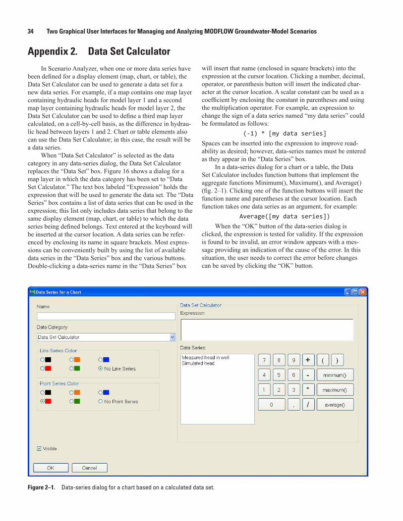
34 Two Graphical User Interfaces for Managing and Analyzing MODFLOW Groundwater-Model Scenarios
Appendix 2. Data Set CalculatorIn Scenario Analyzer, when one or more data series have
been defined for a display element (map, chart, or table), the Data Set Calculator can be used to generate a data set for a new data series. For example, if a map contains one map layer containing hydraulic heads for model layer 1 and a second map layer containing hydraulic heads for model layer 2, the Data Set Calculator can be used to define a third map layer calculated, on a cell-by-cell basis, as the difference in hydrau-lic head between layers 1 and 2. Chart or table elements also can use the Data Set Calculator; in this case, the result will be a data series.
When “Data Set Calculator” is selected as the data category in any data-series dialog, the Data Set Calculator replaces the “Data Set” box. Figure 16 shows a dialog for a map layer in which the data category has been set to “Data Set Calculator.” The text box labeled “Expression” holds the expression that will be used to generate the data set. The “Data Series” box contains a list of data series that can be used in the expression; this list only includes data series that belong to the same display element (map, chart, or table) to which the data series being defined belongs. Text entered at the keyboard will be inserted at the cursor location. A data series can be refer-enced by enclosing its name in square brackets. Most expres-sions can be conveniently built by using the list of available data series in the “Data Series” box and the various buttons. Double-clicking a data-series name in the “Data Series” box
will insert that name (enclosed in square brackets) into the expression at the cursor location. Clicking a number, decimal, operator, or parenthesis button will insert the indicated char-acter at the cursor location. A scalar constant can be used as a coefficient by enclosing the constant in parentheses and using the multiplication operator. For example, an expression to change the sign of a data series named “my data series” could be formulated as follows:
(-1) * [my data series]Spaces can be inserted into the expression to improve read-ability as desired; however, data-series names must be entered as they appear in the “Data Series” box.
In a data-series dialog for a chart or a table, the Data Set Calculator includes function buttons that implement the aggregate functions Minimum(), Maximum(), and Average() (fig. 2–1). Clicking one of the function buttons will insert the function name and parentheses at the cursor location. Each function takes one data series as an argument, for example:
Average([my data series])When the “OK” button of the data-series dialog is
clicked, the expression is tested for validity. If the expression is found to be invalid, an error window appears with a mes-sage providing an indication of the cause of the error. In this situation, the user needs to correct the error before changes can be saved by clicking the “OK” button.
Figure 2–1. Data-series dialog for a chart based on a calculated data set.

Appendix 3 35
Appendix 3. Data FilesScenario Manager and Scenario Analyzer obtain data
from a variety of data file types. The file types are described in following subsections.
Shapefiles
Shapefiles (Environmental Systems Research Institute, Inc., 1998) are used to provide georeferenced information specifying the finite-difference grid used by the model and describing physical features or areas of hydrologic signifi-cance to be simulated. A given shapefile can contain geometric features: points, polylines, or polygons.
Scenario Manager requires a polygon shapefile repre-senting the finite-difference model grid to generate model-input files from points, polylines, or polygons representing groundwater-system features or areas of hydrologic signifi-cance stored in other shapefiles. The discretization process of converting points, polylines, and polygons to cell-based model features requires that the attribute table of the model-grid shapefile include attributes identifying the row and column of each cell. The attribute containing the row number needs to be named “row” or “rownum,” and the attribute containing the column number needs to be named one of the following: “col,” “colnum,” “column,” or “columnnum.” Scenario Ana-lyzer also uses a model-grid shapefile for making maps. The model-grid shapefile needs to contain a polygon for each cell in a model layer, including inactive cells.
Users need to ensure that all shapefiles and georeferenced image files, if used, share a common projected coordinate system. If a conflict or apparent conflict is detected, a warning is issued.
Time-Series Data
Scenario Manager and Scenario Analyzer use time-series data for a number of purposes. The format for text files con-taining time-series data is based on the specification of a “Bore Sample File” as described by Doherty (2011). By default, names of time-series files are assumed to have “smp” as the file extension. The format as supported in Scenario Manager and Scenario Analyzer is summarized here.
Each record of a time-series file contains at least four entries in the following order separated by one or more spaces: (1) identifier, (2) date, (3) time, and (4) value. The tab character can also be used as a delimiter. Commas cannot be used as delimiters. An optional fifth entry (indicating that the record lacks integrity) may be included as described by Doherty (2011), but it is not used by Scenario Manager or Scenario Analyzer.
Identifier is a string of characters associating the record with a particular site or feature. Unlike the Doherty (2011) specification, the length of the identifier is not limited. The string may not include embedded spaces.
Date is an 8- to 10-character string in the format MM/DD/YYYY, where MM consists of one or two characters indicating the month, DD is one or two characters indicating the day number in the month, and YYYY is four characters indicating the year.
Time is a 5- to 8-character string in the format HH:MM:SS, where HH is one or two characters indicating the hour (0 to 24), MM is one or two characters indicating the minute, and SS is one or two characters indicating the second.
Value is a numeric value in floating-point notation. An exponent can be provided using “E” notation. For example 0.0123 can be specified as 1.23E-2.
A time-series file can contain records for multiple identi-fiers, but all similar identifiers need to be grouped together. Records sharing the same identifier need to appear in chrono-logical order.
An example showing the contents of a time-series file follows:
Well_1 6/30/2013 24:00:00 0.0Well_1 07/01/2013 8:00:00 2.7Well_1 07/01/2013 20:00:00 4.5Well_1 07/02/2013 08:00:00 3.1Well_1 07/02/2013 20:00:00 4.0Well_1 07/03/2013 08:00:00 2.5Well_1 07/03/2013 20:00:00 0.0
In some situations, the user has a choice with respect to interpretation of time-series data that will be used by Scenario Manager to generate time-varying input. The user may use either of two methods when interpolation between times pro-vided in the time series is required: stepwise or piecewise linear. This choice affects how stress values for stress-period-by-stress-period input to packages are calculated from time-series data.
For stepwise interpretation, values for times intermedi-ate between times provided in the time series are assumed to equal the value provided in the last record preceding the time of interest. For example, if a value for Well_1 is required on 7/1/2013 at time 14:00:00, Scenario Manager would use the value provided in the last preceding record (Well_1 07/01/2013 8:00:00 2.7), which is 2.7.
For piecewise-linear interpretation, values for times intermediate between times provided in the time series are assumed to vary linearly between the provided times. If we use the same example with a piecewise-linear interpretation, a value required on 7/1/2013 at time 14:00:00 would be linearly interpolated by Scenario Manager as 3.6.
Time-series data are used to control time-varying stress values for each of the packages supported by Scenario Man-ager. During an interval when the stress value for a feature (typically, an elevation or a flow or flux rate) is unchanging, the number of records in a time-series file can be minimized by providing a record at the beginning of the interval and
Appendix 3

36 Two Graphical User Interfaces for Managing and Analyzing MODFLOW Groundwater-Model Scenarios
one at the end of the interval, where each record contains the same stress value. This value will be used for each stress period that starts and ends within the time interval defined by the two records.
Feature sets defined for the River and GHB packages also support the use of a secondary time-series file to control activation and deactivation of features during the course of a simulation, as described in the “River Package” section. An important difference between a secondary time-series file and a time-series file used to define stress values is that a second-ary time-series file needs to include at least one record with a positive value in each stress period in which the feature is to be active. In contrast, if the stress value for a feature is unchanging during multiple stress periods, the time-series file used to define stress values need not contain records cor-responding to individual stress periods, as is described in the preceding paragraph.
Cell Groups
A cell group is a user-defined subset of cells in a 2D, areal representation of the model, which may be used in Sce-nario Analyzer to aggregate data of interest for use in charts and tables. Input defines cells included in a cell group by row and column indices. A given cell group may be applied to one or more model layers. A given cell may be included in more than one cell group. There is no requirement that all cells in a layer belong to a cell group.
Data to define cell groups are read from one or more cell-group files. A cell-group file is a text file containing comma-separated entries, in a form commonly known as a Comma-Separated Value (CSV) file. By convention, the extension “csv” identifies a CSV file.
A cell-group file designed for Scenario Analyzer will contain records of two types: (1) header record, and (2) cell record. A cell group is defined by one header record followed by one or more cell records. A header record has the follow-ing form:
group-namewhere group-name is a text string that will be used to identify the cell group. A cell record has the following form:
row, columnwhere row is the row index and column is the column index (both one-based) of a model cell. A cell-group file may contain one or more cell groups. Consider a model grid of three rows and four columns, with two cell groups identified by the inte-gers 1 and 2:
ColumnRow 1 2 3 41 1 1 1 22 1 1 2 23 1 2 2
The following example shows a cell-group file that contains entries to define the two cell groups:
Cell_group_11,11,21,32,12,23,1Cell_group_21,42,32,43,23,3
Scenario Analyzer keeps a single list of cell-group files and associated cell groups. As a result, if a cell-group file is imported for one data series, that cell-group file and the cell groups defined in the file are available for use with any other data series.
Georeferenced Images
Both Scenario Manager and Scenario Analyzer support the use of a georeferenced raster image. Image files in the pub-lic-domain Geographic Tagged Image File Format (GeoTIFF) have been successfully tested with the programs. The library used for importing a GeoTIFF file is the Geospatial Data Abstraction Library (GDAL) (http://www.gdal.org/). GDAL supports a large number of other file formats for georeferenced raster images; it may be possible to import and display images in some of these formats, but importing files in formats other than GeoTIFF has not been tested. See http://www.gdal.org/formats_list.html for a complete list of file formats supported by GDAL.
Users need to ensure that all shapefiles and georeferenced image files, if used, share a common projected coordinate system. If a conflict or apparent conflict is detected, a warning is issued.
Binary Files Generated by MODFLOW and Related Programs
MODFLOW and related programs can generate binary files of two basic types. Scenario Analyzer can import data sets from either of these types. The first type is used to record values of hydraulic head, drawdown, and solute concentration. The second type is used to record values of flow for individual model cells. These two types are briefly described in the fol-lowing sections.

Appendix 3 37
Head, Drawdown, and Concentration FilesPrograms that solve the groundwater flow equation popu-
late arrays of hydraulic head and drawdown. These arrays may be written to output files in binary form, depending on the con-tents of an Output Control file (Harbaugh, 2005). Hydraulic head and drawdown may be written to separate files, or they may be combined into a single file. SEAWAT and MT3DMS populate arrays of solute concentration, which may be written to output files in binary form; these files may contain only solute-concentration data. Each data set in a file of this type holds one 2D array associated with a particular model layer and a particular time step in the simulation. Each data set also has a data identifier, which can be “HEAD,” “DRAW-DOWN,” or “CONCENTRATION.” When MT3DMS is used to simulate transport of multiple species, each concentration output file contains values for a single species. To import data for a particular species, the user would need to select the file containing values for the species of interest.
Cell-By-Cell Budget FilesPrograms that solve the groundwater flow equation also
can generate a binary file containing values of calculated groundwater flow into and out of individual model cells. Each data set in a file of this type is written by a particular MODFLOW package for a particular model time step and is
identified by a data identifier (table 3–1). Scenario Analyzer reads data identifiers from the cell-by-cell budget file; there-fore, data written by packages not listed in table 3–1 (as would be the case when new packages are added to MODFLOW) will be available for use. A cell-by-cell budget file can be either non-compact or compact.
In a non-compact cell-by-cell budget file, each data set contains a 2D array of data for one model layer. Some MODFLOW packages (for example the RIV, WEL, and GHB Packages) define model boundaries and stresses using lists of cells. When a non-compact budget file is used, these cell-list-based packages write a zero value for model cells not included in the list defined for the package. When data are obtained by Scenario Analyzer from a non-compact cell-by-cell budget file for cell-list-based packages and used to generate a color-fill layer, these zero values will obscure the display of any map layers lower on the list of layers displayed in the analysis design panel of the Scenario Analyzer main window.
In a compact cell-by-cell budget file, each data set written by a cell-list-based package contains data only for cells in the list defined for that package. A single data set will contain data for all cells in the list and may include cells in multiple layers. When data are obtained by Scenario Analyzer from a compact cell-by-cell budget file for cell-list-based packages and used to generate a color-fill layer, the layer will not obscure the dis-play of data in lower map layers where cells are not included in the list.
Table 3–1. Data that may be contained in a cell-by-cell budget file, by MODFLOW package.
MODFLOW package
Data Identifier Description, showing sign convention
Flow1
CONSTANT HEAD Flow into (+) or out of (-) groundwater system at constant-head cells.FLOW RIGHT FACE Flow to (+) or from (-) neighboring cell in next column.FLOW FRONT FACE Flow to (+) or from (-) neighboring cell in next row.FLOW LOWER FACE Flow to (+) or from (-) neighboring cell in next layer.STORAGE Flow to groundwater system from storage (+) or from groundwater system to storage (-).
DRN2 DRAINS Flow out of (-) groundwater system at drain cells.DRT3 DRAINS (DRT) Flow into (+) or out of (-) groundwater system at drain-return cells.ETS4 ET SEGMENTS Flow out of (-) groundwater system at evapotranspiration cells.EVT5 ET Flow out of (-) groundwater system at evapotranspiration cells.FHB6 SPECIFIED FLOWS Flow into (+) or out of (-) groundwater system at specified-flow cells.GHB7 HEAD DEP BOUNDS Flow into (+) or out of (-) groundwater system at general-head boundary cells.
IBS8 INTERBED STORAGE Flow to groundwater system from interbed storage (+) or from groundwater system to interbed storage (-).
LAK9 LAKE SEEPAGE Flow into (+) or out of (-) groundwater system at lake cells.MNW110 MNW Flow into (+) or out of (-) groundwater system at multinode-well cells.MNW211 MNW2 Flow into (+) or out of (-) groundwater system at multinode-well cells.RCH12 RECHARGE Flow into (+) or out of (-) groundwater system at recharge cells.
Appendix 3

38 Two Graphical User Interfaces for Managing and Analyzing MODFLOW Groundwater-Model Scenarios
MODFLOW package
Data Identifier Description, showing sign convention
RES13 RESERV. LEAKAGE Flow into (+) or out of (-) groundwater system at reservoir cells.RIV14 RIVER LEAKAGE Flow into (+) or out of (-) groundwater system at river cells.
SFR215STREAM LEAKAGE Flow into (+) or out of (-) groundwater system at stream reaches.STREAMFLOW OUT Streamflow out (+) of stream reaches.
STR16STREAM LEAKAGE Flow into (+) or out of (-) groundwater system at stream reaches.STREAM FLOW OUT Streamflow out (+) of stream reaches.
SUB17
INST. IB STORAGE Instantaneous flow to groundwater system from interbed storage (+) or from groundwater system to interbed storage (-).
DELAY IB STORAGE Delayed flow to groundwater system from interbed storage (+) or from groundwater system to interbed storage (-).
SWR18SWR LEAKAGE Flow into (+) or out of (-) groundwater system at surface-water routing cells.SWR GWET Flow out of (-) groundwater system as groundwater evapotranspiration.
SWT19 INTERBED STORAGE Flow to groundwater system from interbed storage (+) or from groundwater system to interbed storage (-).
UZF20
UZF RECHARGE Flow into (+) groundwater system from unsaturated zone.GW ET Flow out of (-) groundwater system as groundwater evapotranspiration.SURFACE LEAKAGE Flow into (+) or out of (-) groundwater system at land surface.
WEL21 WELLS Flow into (+) or out of (-) groundwater system at well cells.1 Flow package may be one of: LPF (Layer Property Flow Package; Harbaugh, 2005), BCF (Block-Centered Flow Package; Harbaugh, 2005), HUF
(Hydrologic Unit Flow Package; Anderman and Hill, 2000), or UPW (Upstream Weighting Package; Niswonger and others, 2011)2 Drain Package (Harbaugh, 2005)3 Drain Return Package (Banta, 2000) 4 Evapotranspiration Segments Package (Banta, 2000)5 Evapotranspiration Package (Harbaugh, 2005)6 Flow and Head Boundary Package (Leake and Lilly, 1997)7 General Head Boundary Package (Harbaugh, 2005)8 Interbed Storage Package (Leake and Prudic, 1991) 9 Lake Package (Merritt and Konikow, 2000)10 Multi-NodeWell Package, version 1 (Halford and Hanson, 2002)11 Multi-Node Well Package, version 2 (Konikow and others, 2009)12 Recharge Package (Harbaugh, 2005)13 Reservoir Package (Fenske and others, 1996)14 River Package (Harbaugh, 2005)15 Streamflow-Routing Package, version 2 (Niswonger and Prudic, 2006)16 Stream Package (Prudic, 1989)17 Subsidence Package (Hoffmann and others, 2003)18 Surface-Water Routing Package (Hughes and others, 2012)19 Subsidence and Aquifer-System Compaction Package for Water-Table Aquifers (Leake and Galloway, 2007)20 Unsaturated-Zone Flow Package (Niswonger and others, 2006)21 Well Package (Harbaugh, 2005)
Table 3–1. Data that may be contained in a cell-by-cell budget file, by MODFLOW package.—Continued

Banta—Tw
o Graphical U
ser Interfaces for Managing and A
nalyzing MO
DFLO
W G
roundwater-M
odel Scenarios—Techniques and M
ethods 6–A50
ISSN 2328-7055 (online)http://dx.doi.org/10.3133/tm6a50