Two-dimensional Nanolithography Using Atom Interferometry

A. Gangat, P. Pradhan, G. Pati, and M.S. Shahriar

Deptartment of Electrical and Computer Engineering, Northwestern University, Evanston, IL 60208

Abstract We propose a novel scheme for the lithography of arbitrary, two-dimensional

nanostructures via matter-wave interference. The required quantum control is provided by a π/2- π - π /2 atom interferometer with an integrated atom lens system. The lens system is developed such that it allows simultaneous control over atomic wave-packet spatial extent, trajectory, and phase signature. We demonstrate arbitrary pattern formations with two-dimensional 87Rb wave-packets through numerical simulations of the scheme in a practical parameter space. Prospects for experimental realizations of the lithography scheme are also discussed. PACS: 39.20.+q, 03.75.Dg, 04.80.-y, 32.80.Pj

1

I. INTRODUCTION The last few decades have seen a great deal of increased activity toward the development of a broad array of lithographic techniques [1,[2]. This is because of their fundamental relevance across all technological platforms. These techniques can be divided into two categories: parallel techniques using light and serial techniques using matter. The optical lithography techniques have the advantage of being fast because they can expose the entire pattern in parallel. However, these techniques are beginning to reach the limits imposed upon them by the laws of optics, namely the diffraction limit [3]. The current state-of-the-art in optical lithography that is used in industry can achieve feature sizes on the order of hundreds of nanometers. Efforts are being made to push these limits back by using shorter wavelength light such as x-rays [2], but this presents problems of its own. The serial lithography techniques, such as electron beam lithography [1], can readily attain a resolution on the order of tens of nanometers. However, because of their serial nature these methods are very slow and do not provide a feasible platform for the industrial mass fabrication of nano-devices. A new avenue for lithography presents itself out of recent developments in the fields of atomic physics and atom optics, namely the experimental realization of Bose-Einstein Condensation (BEC) - ] and the demonstration of the atom interferometer [7- ]. In essence, these developments provide us with the tools needed in order to harness the wave nature of matter. This is fortuitous for lithography because the comparatively smaller de Broglie wavelength of atoms readily allows for a lithographic resolution on the nanometer scale. The atom interferometer provides a means of interfering matter waves in order to achieve lithography on such a scale. The BEC, on the other hand, provides a highly coherent and populous source with which to perform this lithography in a parallel fashion. The opportunity thus presents itself to combine the enhanced resolution of traditional matter lithography with the high throughput of traditional optical lithography.

[4 [5[6[13

[13

In this paper we seek to demonstrate the viability of using the atom interferometer as a platform for nanolithography by proposing a scheme that allows for the manipulation of a single atomic wavepacket so as to achieve two-dimensional lithography of an arbitrary pattern on the single nanometer scale. The rest of this section gives an overview of the proposal. Sec. II and III provide detailed theoretical analysis of the atom interferometer itself and our proposed imaging system, respectively. Sec. IV is devoted to some practical considerations of the setup and its parameter space, and Sec. V gives the results of numerical simulations. Finally, we touch upon the issue of incorporating BEC into such a system in Sec. VI.

I. A. π/2 - π - π/2 Atom interferometer

In a π/2 - π - π/2 atom interferometer (AI) [7 ], as illustrated in Fig.1, an atom beam, consisting of non-interacting atomic wavepackets, is released from its source and allowed to propagate in vacuum. Typically, it is dropped vertically so as to accelerate only due to gravity. If the direction of propagation is along the z axis, the wavepackets will have a finite extent in the x-y plane. As it travels, the beam is first split into two

2

separate but equally populated sub-beams using what is effectively an atom beam splitter - ]. This beam splitter results from a specific laser field configuration denoted as a

π/2 pulse. After some propagation time, the sub-beams are reflected such that their trajectories now intercept. The effective atom mirror that causes the reflection is also a specific laser field configuration termed a π pulse. At the place of intersection, the sub-beams are again exposed to a π/2 pulse, which in this case acts as a beam combiner and causes the sub-beams to mix their populations among the two trajectories. Some further distance away, one or both trajectories of the now mixed sub-beams are intercepted by a substrate in the x-y plane. Due to the mixing caused by the last π/2 pulse, any phase difference introduced between the two sub-beams before they are mixed results in an intensity modulation of the mixed sub-beams as observed on the substrate, the intensity being proportional to the cosine of the phase difference. Thus, we see that the π/2 - π - π/2 atom interferometer is akin to the Mach-Zehnder interferometer ] from classical optics.

[14 [20

[21

I. B. Image Formation As mentioned above, the atomic wavepackets have a finite extent in the transverse plane. This allows for a phase shift introduced along one of the sub-beams to also be a function of x and y. Since the mixed sub-beam intensity at the substrate depends on the phase difference ( yx, )φ between the two sub-beams before they are mixed, a fortuitous choice of ( yx, )φ can yield a sub-beam intensity profile of our choice that is a function of x and y. If sufficient deposition time is allowed, the distribution of the atoms on the substrate will follow the mixed sub-beam intensity profile. Thus, the formation of an arbitrary pattern will occur.

As an example, consider the introduction of a phase shift that is linear in x and constant in y to one of the sub-beams right before the final π/2 pulse. This will yield a mixed sub-beam intensity profile that varies sinusoidally in x and stays constant in y, thereby forming a physical grating. More specifically, if we take ( ) xyx πϕ 4, = to be the phase difference between the two arms of the AI, the resulting beam intensity at the substrate at (6) in Fig. 1 will be proportional to ( )xπ4cos . I. C. The Overall Scheme In our overall scheme, represented by Fig. 2, atoms are prepared in the ground state (purple) at the top of a vacuum chamber, and are treated as three-level lambda systems - ] as shown in the energy level diagram. Our scheme requires precision control of a single wavefunction, so a single atom trap is used to deposit just one atom at a time into the chamber - ]. It may happen that the freespace drop distance for the atom will not provide a large enough time window for proper operation of the lens system. This problem can be alleviated by countering the force of gravity with a magnetic field (black curves), thereby causing the atom to take longer to drop through the chamber. The first π/2 pulse, denoted by the top-most green arrow, splits the

[22 [29

[30 [32

3

wavepacket. The π pulse at the next green arrow causes the two split components to transition their internal states. The component along the right arm is now in the original ground state and is exposed to the lens system. These lenses (red) are pulses of light that enter the chamber from the top and intercept the purple state wavepacket at different times. As seen from the energy level diagram, the detuning of the light that the lenses are composed of is several times larger for the green state than for the purple state. The lenses can therefore be considered to have a negligible ac-stark effect on the green state as compared to the purple state. The same is the case for the pattern phase. The pulse of light for the pattern phase is prepared by passing it through an intensity mask that is proportional to the inverse cosine of the arbitrary pattern (normalized to 1). Just as with the lenses, the light pulse for the pattern phase enters the vacuum chamber from above and intercepts the purple state in the second half of the interferometer at precisely the right moment (denoted by the blue-white rectangle). The last π/2 pulse (bottom green arrow) mixes the two arms of the interferometer, and a SAM-coated wafer intercepts just the purple state, which is now composed of two components that have each traveled along a different arm of the interferometer and thus have a phase difference given by the pattern phase. This phase difference causes an interference at the wafer that goes as the cosine of the phase difference, which results in the formation of the arbitrary pattern. So that the wafer does not cause reflection of the light pulses that form the lenses and the pattern phase mask, it is moved into place after the pulses have passed through. Finally, the pattern can be transferred to a more viable medium through standard chemical procedures ]. [33 II. Analysis of the Interferometer II. A. Formalism In our formulation of the problem, we consider the behavior of a single atom. This is possible because the atoms in the atom beam are assumed to be non-interacting. Also, in order to understand and simulate the AI - ] properly, the atom must be modeled both internally and externally. As we will show below, this is primarily because the internal and external states of the atom are entangled. It is the internal evolution of the atom while in a laser field that allows for the splitting and redirecting of the beam to occur in the AI. However, the internal evolution is also dependent on the external state. Also, while the external state of the atom accounts for most of the interference effects which result in the arbitrary pattern formation, the internal state is responsible for some nuances here as well. Both internal and external state evolution are governed by the Schrodinger equation (SE):

[7 [13

Ψ=∂Ψ∂

Ht

ih (1)

4

In following the coordinate system of Fig. 1, we write the initial external wavefunction as:

( )

−==Ψ 2

2

2exp10,

σπσ

rtre

vv (2)

where jyixr ˆˆ +=v . Our use here of a two-dimensional model is justified because no measurement is made in the z direction. Internally, the atom is modeled as a three level lambda system - ] and is assumed to be initially in state 1 : [22 [28

( ) 3)(2)(1)( 321 tctctcti ++=Ψ , (3) where 0)0(,0)0(,1)0( 321 === ccc . States 1 and 3 are metastable states, while state

2 is an excited state. Fig. 3 gives an illustration of the external and internal models of the atom. As will become evident later, in some cases it is more expedient to express the atom’s wavefunction in k-space ]. To express our wavefunction, then, in terms of momentum, we first use Fourier theory to re-express the external wavefunction as:

[34

( ) ( ) yxykxki

yxee dkdketkktyx yx∫∫ +Φ=Ψ )(,,21,,π

, (4a)

( ) ( ) dydxetyxtkk ykxkieyxe

yx )(,,21,, +−∫∫ Ψ=Φπ

. (4b)

Now, (recalling that ) if we let kp h=x

pi

x

x

ep h= and y

pi

y

y

ep h= , then we can write:

( ) ( ) yxyxyxee dpdppptpptyx ∫∫ Φ=Ψ ,,21,,π

, (5a)

( ) ( ) dydxetyxtppy

px

pi

eyxe

yx )(,,

21,, hh

+−

∫∫ Ψ=Φπ

. (5b)

5

The complete wavefunction is simply the outer product of the internal and external states (Eq. (3) and (5a)):

( ) ( ) ( )[∫∫ +=Ψ yxyxyxyx pptppCpptppCtyx ,,2,,,,1,,21,, 21π

( ) ] ,,,3,,3 yxyxyx dpdppptppC+ (6) where ( ) ( ) ( )tpptctpp yxenyxn ,,,, Φ=C . In position space, the outer product gives:

( ) ( ) ( ) ( ) ( ) ( ) ( )trtctrtctrtctr eee ,,3,,2,,1, 321vvvv Ψ+Ψ+Ψ=Ψ . (7)

II. B. State Evolution in Freespace

In freespace, the Hamiltonian can be expressed in the momentum domain as:

yxn

yxyxnyx dpdpppnppn

mpp

H ∫∫∑=

+

+=

3

1

22

,,,,2

ωh . (8)

Where nω is the frequency corresponding to the eigenenergy of internal state n . For a single momentum component ( 0xx pp = and 0yy pp = ), the Hamiltonian in matrix form is:

.

200

02

0

002

3

20

20

2

20

20

1

20

20

++

++

++

=

ω

ω

ω

h

h

h

mpp

mpp

mpp

H

yx

yx

yx

(9)

Using this in Eq. (1), we get the equations of motion as:

6

( ) ( )

( ) (

( )

)

( ).,,2

,,

,,,2

,,

,,,2

,,

0033

20

20

003

0022

20

20

002

0011

20

20

001

tppCm

ppitppC

tppCm

ppitppC

tppCm

ppitppC

yxyx

yx

yxyx

yx

yxyx

yx

+

+−=

+

+−=

+

+−=

ω

ω

ω

hh

&

hh

&

hh

&

(10)

These yield the solutions:

( ) ( )

( ) ( )

( ) ( ) .0,,,,

,0,,,,

,0,,,,

3

20

20

2

20

20

1

20

20

2003003

2002002

2001001

tm

ppi

yxyx

tm

ppi

yxyx

tm

ppi

yxyx

yx

yx

yx

eppCtppC

eppCtppC

eppCtppC

+

+−

+

+−

+

+−

=

=

=

ω

ω

ω

h

h

h

(11)

We see that if the wavefunction is known at time 0=t , then after a duration of time T in freespace, the wavefunction becomes:

( ) ( )∫∫

==Ψ

+

+−

yx

Tm

ppi

yx ppeppCTtryx

,,10,,21,

1

22

21

ω

πhv

( ) yx

Tm

ppi

yx ppeppCyx

,,20,,2

22

22

+

+−

+ω

h

( ) yxyx

Tm

ppi

yx dpdpppeppCyx

+

+

+−

,,30,,3

22

23

ωh

. (12a)

We can also write it as:

( ) ( ) ( ) ( ) ( )( ) ( )Trce

TrceTrceTtr

eTi

eTi

eTi

,,30

,,20,,10,

3

21

3

21

v

vvv

Ψ+

Ψ+Ψ==Ψ−

−−

ω

ωω

(12b)

7

II. C. State Evolution in π and π/2 pulse laser fields The electromagnetic fields encountered by the atom at points 2, 3, and 5 in Fig. 1 that act as the π and π/2 pulses are each formed by two lasers that are counter-propagating in the y-z plane parallel to the y axis. We will refer to the laser propagating in the +y direction as AE

v, and the one propagating in the –y direction as BE

v. In deriving the

equations of motion under this excitation, we make the following assumptions: (1) the laser fields can be treated semi-classically ], (2) the intensity profiles of the laser fields forming the π and π/2 pulses remain constant over the extent of the atomic wavepacket (Fig. 4(a-c)), (3) the wavelengths of the lasers are significantly larger than the separation distance between the nucleus and electron of the atom, (4) AE

vexcites only

the 21 ↔ transition and BEv

only the 23 ↔ transition (Fig. 5), (5) AEv

and BEv

are

far detuned from the transitions that they excite, and (6) AEv

and BEv

are of the same intensity.

[35

Using assumptions 1) and 2), we write the laser fields as:

( )

[ )ˆ()ˆ(0

0

2

ˆcos

AAAAAA yktiyktiA

AAAAA

eeE

yktEE

φωφω

φω

+−−+− +=

+−=v

]

vv

(13a)

and

( )

[ )ˆ()ˆ(0

0

2

ˆcos

BBBBBB yktiyktiB

BBBBB

eeE

yktEE

φωφω

φω

++−++ +=

++=v

]

vv

, (13b)

where 0AE

v and 0BE

v are vectors denoting the magnitude and polarization of their

respective fields. Keeping in mind that our wavefunction is expressed in the momentum domain, we take position as an operator. The Hamiltonian here is expressed as the sum of two parts: . The first part, given in the previous section as Eq. (8), corresponds to the non-interaction energy. We repeat it here for convenience:

10 HHH +=

yxn

yxyxnyx dpdpppnppn

mpp

H ∫∫∑=

+

+=

3

1

22

0 ,,,,2

ωh . (14)

8

The second part accounts for the interaction energy, for which we use assumption (3) from above to make the electric dipole approximation and get:

[ ]

[ ])ˆ()ˆ(00

)ˆ()ˆ(001

2

2

BBBBBB

AAAAAA

yktiyktiB

yktiyktiA

eeE

e

eeE

eH

φωφω

φωφω

ε

ε

++−++

+−−+−

+•−

+•−=v

v

vv

, (15)

whereεv is the position vector of the electron, and is the electron charge. Now, seeing that expressions of the form

0enEn A0

vv •ε and nEn B0

vv •ε are zero, and using assumption (4), we can express Eq. (15) as:

[ ]∫∫

+

+= +−−+− )ˆ()ˆ(

1,,1,,2

,,2,,1

2AAAAAA yktiykti

yxyx

yxyxA eepppp

ppppgH φωφωh

[ ] yxyktiykti

yxyx

yxyxB dpdpeepppp

ppppgBBBBBB

+

++ ++−++ )ˆ()ˆ(

,,3,,2

,,2,,3

2φωφωh , (16)

where we let 1221 00 AAA EEg

vvvv •=•= εε and 3223 00 BBB EEgvvvv •=•= εε .

Finally, we can use the identities ]. [34

yxn

yxyxyik dpdpkppnppne ∑∫∫ −= h,,,,ˆ (17a)

and

yxn

yxyxyik dpdpkppnppne ∑∫∫ +=− h,,,,ˆ , (17b)

and the rotating wave approximation ] in Eq. (16) to give: [35

∫∫ += +

AyxyxtiA kppppe

gH AA h

h,,2,,1

2)(

1φω

9

yxAyxtiA ppkppeg

AA ,,1,,22

)( hh

++ +− φω

AyxBAyxtiB kppkkppeg

BB hhhh

++++ + ,,2,,32

)( φω

yxAByxAyxtiB dpdpkkppkppeg

BB

++++ +− hhh

h ,,3,,22

)( φω . (18)

We note that the full interaction between the internal states ,2,1 and 3 occurs

across groups of three different momentum components: ,,,, Ayxyx kpppp h+ and

BAyx kkpp hh ++, . Fig. 5 shows one such momentum manifold. This can be understood physically in terms of photon absorption/emission and conservation of momentum. Keeping in mind assumption (4), if an atom begins in state 00 ,,1 yx pp and absorbs a

photon from field AEv

, it will transition to internal state 2 because it has become excited, but it will also gain the momentum of the photon (h ) traveling in the +y direction. It will therefore end up in state

Ak

Ayx kpp h+00 ,,2 . Now the atom is able to

interact with field BEv

, which can cause stimulated emission of a photon with momentum in the –y direction. If such a photon is emitted, the atom itself will gain an equal

momentum in the opposite direction, bringing it into external state Bkh

BAyx kkpp hh ++00 , .

The atom will also make an internal transition to state 3 because of the de-excitation.

The total state will now be BAyx kkpp hh ++00 ,,3 . We thereby see that our mathematics is corroborated by physical intuition.

Getting back to the Hamiltonian, we look at the general case of one momentum grouping so that we get in matrix form 10 HHH += from equations (14) and (18):

( )

( ).

220

222

022

3

22)(

)(2

22)(

)(1

22

++++

+++

++

=

+

+−+−

+

ω

ω

ω

φω

φωφω

φω

hhhh

hh

hh

hh

mkkpp

eg

eg

mkpp

eg

eg

mpp

H

BAyxtiB

tiBAyxtiA

tiAyx

BB

BBAA

AA

(19)

In order to remove the time dependence we apply some transformation Q ] of the form:

[34

10

=+

+

+

)(

)(

)(

33

22

11

000000

φθ

φθ

φθ

ti

ti

ti

ee

eQ , (20)

so that Eq. (1) becomes

Ψ=∂

Ψ∂ ~~~

Ht

ih , (21)

where Ψ=Ψ Q~ and 11~ −−

∂∂

+= QtQiQHQH h . The matrix representation is:

( )

( )( )

( )(( )

+++=

+++=Ψ

+

+

+

tkkppCetkpppCe

tppCe

tkkppCtkppC

tppC

BAyxti

Ayyxti

yxti

BAyx

Ayx

yx

,,,,

,,

,,~,,~

,,)

~~

3)(

2)(

1)(

3

2

1

33

22

11

hh

h

hh

hφθ

φθ

φθ

(22)

and

( )

( ).

220

222

022

~

33

22)()(

)()(22

22)()(

)()(11

22

2323

23232121

2121

−++++

−+++

−++

=

−++−+

−+−−+−−+−−+−

−++−+

θω

θω

θω

φφφθθω

φφφθθωφφφθθω

φφφθθω

hhhhh

hhh

hh

hhh

mkkpp

eg

egm

kppeg

egm

pp

H

BAyxitiB

itiBAyxitiA

itiAyx

BB

BBAA

AA

(23) Choosing ,0, 21 =−= θωθ A Bωθ −=3 , Aφφ −=1 , 02 =φ , and Bφφ −=3 , Eq. (23) becomes:

( )( )

( )

++

+

++

=

ByxB

Byx

A

AAyx

ppEg

gppE

g

gppE

H

ωω

ω

ωω

hhh

hh

h

hhh

33

22

11

,2

02

,2

02

,

~ , (24)

11

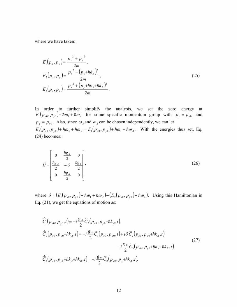
where we have taken:

( ) ,2

,22

1 mpp

ppE yxyx

+=

( ) ( )m

kppppE Ayx

yx 2,

22

2

h++= , (25)

( ) ( )m

kkppppE BAyx

yx 2,

22

3

hh +++= .

In order to further simplify the analysis, we set the zero energy at

( ) Ayx ppE ωω hh ++ 1001 ,

0yy pp = A

for some specific momentum group with and . Also, since

0xx pp =

ω and Bω can be chosen independently, we can let ( ) ( ) AyxByx ppEppE ωωωω hhhh ++=++ 10013003 ,, . With the energies thus set, Eq.

(24) becomes:

−=

02

022

02

0

~

B

BA

A

g

gg

g

H

h

hh

h

δ , (26)

where ( )( ) ( )( )20021001 ,, ωωωδ hhh +−++= yxAyx ppEppE . Using this Hamiltonian in Eq. (21), we get the equations of motion as:

( ) ( )

( ) ( ) ( )

( )

( ) ( ).,,~2

,,~

,,,~2

,,~,,~2

,,~

,,,~2

,,~

02003

003

002001002

002001

tkppCgitkkppC

tkkppCgi

tkppCitppCgitkppC

tkppCgitppC

AyxB

BAyx

BAyxB

AyxyxA

Ayx

AyxA

yx

hhh&

hh

hh&

h&

+−=++

++−

++−=+

+−=

δ (27)

12

Assumption (5) allows us to make the adiabatic approximation so that we can set ( 0,, )~

002 ≈tppC yx& , and assumption (6) gives us 0ggg BA == . The Eqs. (27) then

simplify to:

( ) ( ) ( )

( ) ( ) ( ),,,~4

,,~4

,,~

,,,~4

,,~4

,,~

003

20

001

20

003

003

20

001

20

001

tkkppCg

itppCg

itkkppC

tkkppCg

itppCg

itppC

BAyxyxBAyx

BAyxyxyx

hhhh&

hh&

++−−=++

++−−=

δδ

δδ (28)

where we have chosen to neglect state C from here on due to the adiabatic approximation. We can now use another transformation on this system to make it more tractable. Let:

2

( ) ( )

( ) ( ) .,,~,,~~

,,,~,,~~

4003003

4001001

20

20

tg

i

BAyxBAyx

tg

i

yxyx

etkkppCtkkppC

etppCtppC

δ

δ

hhhh ++=++

= (29)

. The system in Eqs. (28) then becomes:

( ) ( )

( ) ( ).,,~~

4,,

~~

,,,~~

4,,

~~

001

20

003

003

20

001

tppCg

itkkppC

tkkppCg

itppC

yxBAyx

BAyxyx

δ

δ

−=++

++−=

hh&

hh&

(30)

The solution is easily found to be:

13

( )

( )

( ) ( )

( ) ( ).

20,,

~~0,,~~~~

,2

0,,~~0,,

~~~~

,~~~~,,

~~

,~~~~,,

~~

003001

003001

44003

44001

20

20

20

20

BAyxyx

BAyxyx

tg

itg

i

BAyx

tg

itg

i

yx

kkppCppCB

kkppCppCA

eBeAtkkppC

eBeAtppC

hh

hh

hh

+++=

+++−=

+=++

+−=

−

−

δδ

δδ

(31)

When we reverse the transformations given by Eqs. (29) and (20), we get in the original basis:

( )

( )

( ) ( )

( ) ( ),

20,,0,,

,2

0,,0,,

,,,

,,,

2003

2001

2003

2001

222003

222001

BBAA

BBAA

BB

AA

iti

BAyx

iti

yx

iti

BAyx

iti

yx

titiiti

BAyx

titiiti

yx

ekkppCeppCB

ekkppCeppCA

BeAeetkkppC

BeAeetppC

φωφω

φωφω

φω

φω

−

Ω

−−−

Ω

−−

−

Ω

−−−

Ω

−−

Ω−

Ω+

Ω

−

Ω−

Ω+

Ω

−

+++=

+++−=

+=++

+−=

hh

hh

hh

(32)

where we let δ2

20g

=Ω . Finally, substituting in A and B we arrive at:

14

( ) ( )

( )

( ) ( )

( ) .2

cos0,,

2sin0,,,,

,2

sin0,,

2cos0,,,,

003

2001

2003

2003

2

001001

Ω+++

Ω−=++

Ω++−

Ω=

−

Ω

−−+

Ω

−

−

Ω

−−+

Ω

−

tkkppC

teppCietkkppC

tekkppCie

tppCtppC

BAyx

iti

yx

iti

BAyx

iti

BAyx

iti

yxyx

AABB

BBAA

hh

hh

hh

φωφω

φωφω

(33)

It should be noted, however, that these solutions were arrived at only for the specific momentum group where and 0xx pp = 0yy pp = . This was the case where both laser fields were equally far detuned. Other momentum groups will have slightly different solutions due to the Doppler shift, which causes the detunings to be perturbed. For a more accurate description, we need to numerically solve each momentum group’s original three equations of motion without making any approximations. This is what we do in our computational model. For a basic phenomenological understanding of the interferometer, however, it is sufficient to assume that the above analytical solution is accurate for all momentum components. As an approximate expression, then, if the external state of the atom is known at time t , and the atom begins completely in state 0= ( )tre ,,1 vΨ , then after a time T under this excitation, the complete wavefunction from Eq. (6) becomes:

( ) ( )∫∫

Ω==Ψ yxyx ppTppCTtr ,,1

2cos0,,

21, 1π

v

( ) ( ) ( ) yxBAyxyxiTi dpdpkkppTppCie ABAB

++

Ω− −+− hh,,3

2sin0,,1

φφωω

( ) ( ) ( ) ( ) ,0,,32

sin0,,12

cos )( ykkie

iTie

BAABAB erTierT +−−+− Ψ

Ω−Ψ

Ω= vv φφωω

(34) where we have used the definitions given in the “formalism” section above. The phase shift is from the shift in momentum space. We see that if ykki BAe )( +− Ω= /πT , Eq. (34) becomes:

15

( ) ( ) ( ) ( ) ykkie

iiBA

ABAB eyxietyx )(0,,,3/,, +−−+Ω

−Ψ−=Ω=Ψ

φφπ

ωωπ , (35)

while if )2/( Ω= πT , Eq. (34) yields:

( ) ( )

( ) ( ) ( ) .0,,,32

1

0,,,12

1)2/(,,

)(2 ykkie

ii

e

BAABAB eyxie

yxtyx

+−−+Ω

−Ψ−

Ψ=Ω=Ψ

φφπ

ωω

π (36)

It can similarly be shown that if the atom begins completely in state ( )tre ,,3 vΨ , the wavefunction after a time T becomes:

( ) ( ) ( ) ( )

( ) ,0,,,32

cos

0,,,12

sin,, )(

yxT

eyxTieTtyx

e

ykkie

iTi BABABA

Ψ

Ω+

Ψ

Ω−==Ψ +−+− φφωω

(37)

so that if Ω= /πT , Eq. (37) gives:

( ) ( ) ( ) ( ) ykkie

iiBA

BABA eyxietyx )(0,,,1/,, +−+Ω

−Ψ−=Ω=Ψ

φφπ

ωωπ , (38)

while if )2/( Ω= πT , Eq. (37) becomes:

( ) ( ) ( ) ( )

( ) .0,,,32

1

0,,,12

1)2/(,, )(2

yx

eyxietyx

e

ykkie

iiBA

BABA

Ψ+

Ψ−=Ω=Ψ +−+Ω

− φφπ

ωωπ

(39)

We see that an exposure of the wavepacket to the given field for a time )2/( Ω= πT causes it to split equally into two components. This is the “ 2/π pulse.” Also, an exposure to the field for a time Ω= /πT causes the wavepacket to switch its internal state completely. This is the “π pulse.” A transition in the internal state of the atom

16

involves a change in momentum in the +y direction due to photon recoil. After a 2/π pulse, only half of the wavepacket has made a transition in its internal state, and therefore only half of it changes its momentum. The 2/π pulse therefore causes the original wavepacket to split spatially into two equal parts. After a π pulse, the entire wavepacket has made a transition in its internal state, and so the whole of it changes its momentum. The π pulse therefore causes the wavepacket to deflect.

3 3

3 1

1

aΨ

bΨ

II. D. State Evolution Through the Complete Interferometer

Within the context of the whole interferometer, then, referring to Fig. 1, the π/2 pulse at (2) causes the atomic wavepacket, which is initially in state 1 , to go half into

state and remain half in state 1 . The state component separates from the state

1 component due to the additional momentum it gained in the +y direction from photon

recoil. At (3a) the state 3 component encounters a π pulse, which converts it

completely into state 1 . Photon recoil returns it to its original momentum state. At the

same time at (3b), the state 1 component observes a π pulse also, and goes completely

in to state 3 , thus gaining a momentum in the +y direction. The two components of the atomic wavepacket now begin to converge. At (5), the π/2 pulse splits each component. Half of the wavepacket that is in state 1 goes into state and half remains in state .

Similarly, half of the wavepacket that is in state 3 remains in state 3 and half goes

into state 1 . After (5), therefore, the wavepacket in state 3 is now a superposition of parts that traveled along either arm of the AI. The same is true for the wavepacket in state .

To see this more explicitly, we make use of the analysis that we have done for the state evolution of the wavepacket. Take our initial wavepacket Ψ to have initial conditions as discussed in the “formalism” section. At time t=0 the first π/2 pulse equally splits Ψ into two components aΨ and bΨ such that:

( ) ( ) ( ) ykkie

iiBA

ABAB eyxie )(2 0,,,32

111 +−−+Ω

−Ψ−=

φφπ

ωω (40a)

( )0,,,12

1 yxeΨ= , (40b)

where we used Eq. (34). After a time t=T of freespace (Eq. (12b)) and then a π pulse, Eqs. (34) and (37) yield:

0

17

( ) ( ) ( )00

2 ,,,12

1= 032112 Tyyxe e

Tiii

aBBAABA

−Ψ−Ψ−−+−+

Ω− ωφφφφ

πωω

(41a)

( ) ( ) ( ) ykkie

Tiii

bBA

ABAB eTyxie )(0,,,3

210122 +−−−+

Ω−

Ψ−=Ψωφφ

πωω

. (41b)

The aΨ component becomes shifted in space by due to the momentum it gained in the +y direction from the π pulse. Now another zone of freespace for a time T (Eq. (12b)) followed by the final π/2 pulse (using Eqs. (34) and (37)) forms:

0y

0

( ) ( ) ( ) ( )

( ) ( ) ( ) ykkie

Tii

e

Tiii

a

BABBBAAA

BBAABA

eTyyxie

Tyyxe

)(00

002

2,,,321

2,,,121

031321312

0312112

+−+−+−+−−

+−−+−+Ω

−

−Ψ+

−Ψ−=Ψ

ωωφφφφφφ

ωωφφφφπ

ωω

(42a)

and

( ) ( ) ( ) ( )

( ) ( ) ( ) ( ) .2,,,321

2,,,121

)(00

002

03122

0313232

ykkie

Tiii

e

Tiii

b

BAABAB

AABBAB

eTyyxie

Tyyxe

+−+−−+Ω

−

+−+−−+Ω

−

−Ψ−

−Ψ−=Ψ

ωωφφπ

ωω

ωωφφφφπ

ωω

(42b)

Now the bΨ component is spatially aligned with the aΨ component. However,

another split occurs because both of these components are partially in internal state 3 .

After some further time T in freespace, state 1 3 has drifted further in the +y direction. The substrate can now intercept the two internal states of the total wavefunction in separate locations. We write the state 1 wavefunction as:

( ) ( ) ( ) ( )

+−=Ψ

−+−+Ω

−+−−+Ω

− 21123232 221 2

1 BBAABAAABBAB iiiiee

φφφφπ

ωωφφφφπ

ωω

(43a) ( ) ( ) 031

100 2,,,1 Tie eTTyyx ωω +−+−Ψ×

18

and the state 3 wavefunction as:

( ) ( ) ( )

−=Ψ

−+Ω

−+−+−− 22321312

21

3ABAB

BBBAAAiii eei

φφπ

ωωφφφφφφ

(43b) ( ) ( ) 031)(

1010 2,,,3 Tiykkie

BAeTTyyyx ωω +−+−+−−Ψ× These have populations:

( )( ) ( )( ,cos121,cos1

21

033011 φφ −=ΨΨ+=ΨΨ ) (44)

where ( ) 3322110 22 BABABABA φφφφφφωωπφ +−−++−−Ω

=

0

. We see that the state

populations are functions of the phase differences of the laser fields. Since we can choose these phase differences arbitrarily, we can populate the states arbitrarily. If we choose the phases, for example, such that φ is some multiple of 2π, then the wavepacket population will end up entirely in internal state 1 . III. Arbitrary Image Formation

If, however, between the π pulse and second π/2 pulse (corresponding to (4) in Fig. 1) we apply a spatially varying phase shift ( )rP

vφ to aΨ , but keep 0φ as a multiple of 2π, then the populations in Eqs (44) become instead:

( )( )( ) ( )(( rr PPvv φφ cos1

21,cos1

21

3311 −=ΨΨ+=ΨΨ )) . (45)

Therefore, if we let ( ) ( )( )rPrP

vv arccos=φ , where ( )rP v is a normalized arbitrary pattern, the state 1 population will be:

( )( rP v+=ΨΨ 121

11 ) . (46)

19

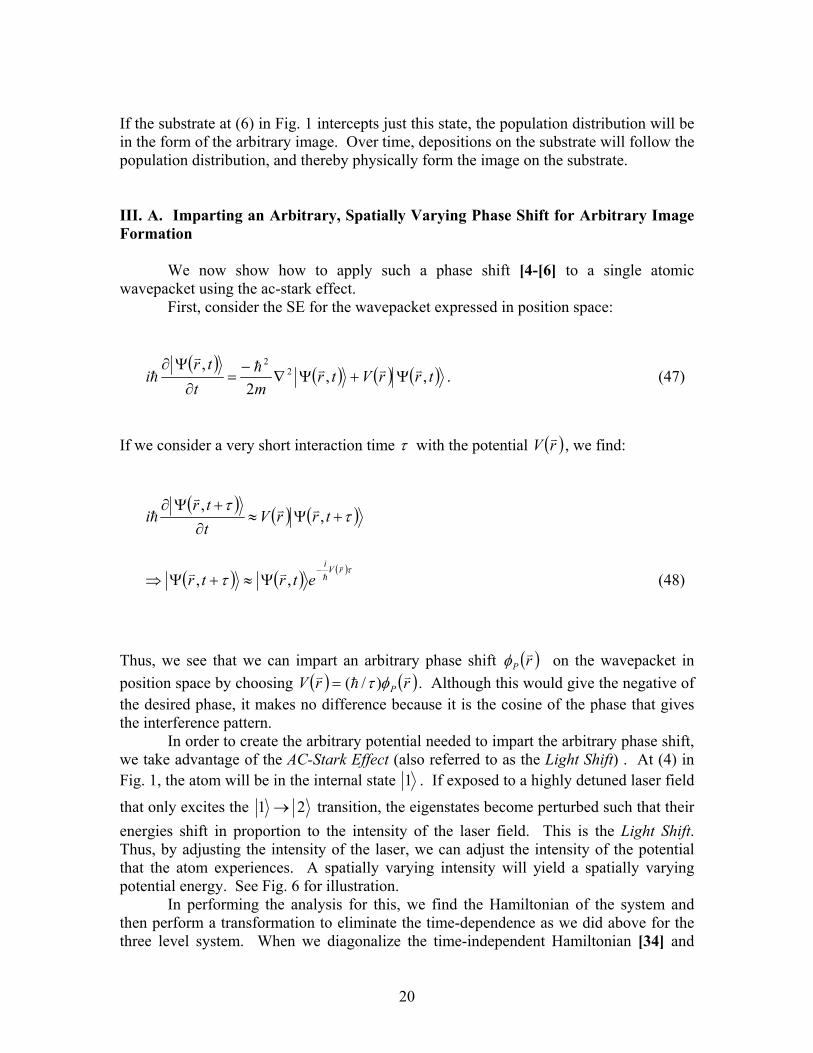
If the substrate at (6) in Fig. 1 intercepts just this state, the population distribution will be in the form of the arbitrary image. Over time, depositions on the substrate will follow the population distribution, and thereby physically form the image on the substrate. III. A. Imparting an Arbitrary, Spatially Varying Phase Shift for Arbitrary Image Formation We now show how to apply such a phase shift - ] to a single atomic wavepacket using the ac-stark effect.

[4 [6

First, consider the SE for the wavepacket expressed in position space:

( ) ( ) ( ) ( )trrVtrmt

tri ,,

2, 2

2 vvvhv

h Ψ+Ψ∇−

=∂

Ψ∂. (47)

If we consider a very short interaction time τ with the potential ( )rV v , we find:

( ) ( ) ( )ττ+Ψ≈

∂+Ψ∂

trrVttr

i ,, vvv

h

( ) ( ) ( )ττ

rVi

etrtrv

hvv −Ψ≈+Ψ⇒ ,, (48)

Thus, we see that we can impart an arbitrary phase shift ( )rP

vφ on the wavepacket in position space by choosing ( ) ( )rr PV v

hv φτ )/(= . Although this would give the negative of

the desired phase, it makes no difference because it is the cosine of the phase that gives the interference pattern.

In order to create the arbitrary potential needed to impart the arbitrary phase shift, we take advantage of the AC-Stark Effect (also referred to as the Light Shift) . At (4) in Fig. 1, the atom will be in the internal state 1 . If exposed to a highly detuned laser field

that only excites the 21 → transition, the eigenstates become perturbed such that their energies shift in proportion to the intensity of the laser field. This is the Light Shift. Thus, by adjusting the intensity of the laser, we can adjust the intensity of the potential that the atom experiences. A spatially varying intensity will yield a spatially varying potential energy. See Fig. 6 for illustration. In performing the analysis for this, we find the Hamiltonian of the system and then perform a transformation to eliminate the time-dependence as we did above for the three level system. When we diagonalize the time-independent Hamiltonian ] and [34

20

make the assumption that 0/ →δg , where g is proportional to the square root of the laser intensity and δ is the detuning, we find that the eigenenergy of the ground state in the transformed basis is approximately ( )δ4/2gh . Due to the adiabatic following ] , we can assume the atom to be completely in this ground state, and since is directly proportional to the laser field intensity we have a direct mapping between the field intensity and the ground state potential energy.

2g[35

To impart the pattern phase, then, we subject the atomic wavepacket at (4) in Fig. 1 to a laser field that has an intensity variation in the x-y plane such that:

( ) ( )( )( rP

rrg Pv )

vv

arccos)/4()/4(2

τδφτδ

==

(49)

where is the normalized arbitrary pattern and ( )rP v t∆ is the interaction time. Fig. 7 illustrates. III. B. The Need for a Lens System The need for a lens system for the atomic wavepacket arises due to two separate considerations. First, there is a need for expanding and focusing the wavepacket in order to shrink down the phase pattern imparted at (4) in Fig. 1. We have shown above how the phase pattern is imparted using an intensity variation on an impinging light pulse. However, due to the diffraction limit of light, the scale limit of this variation will be on the order of 100nm. This will cause the interference at (6) to occur on that scale. To reach a smaller scale, we require a lens system that allows expansion and focusing of the wavepacket to occur in the transverse plane. Using such a system, we could expand the wavepacket by two orders of magnitude prior to (4), impart the phase pattern at (4), and then focus it back to its original size by the time it reaches (6). The interference would then occur on the scale of 1 nm.

The second consideration which must be made is that an arbitrary phase shift φ(x,y) introduced at (4), if it has any variation at all in the transverse plane, will cause the wavepacket traveling along that arm of the AI to alter its momentum state. For example, we know from Fourier theory that a linear phase shift in position space will cause a linear shift in momentum space. Similarly, a complicated phase shift will cause a complicated alteration to the wavepacket’s momentum components. Any freespace evolution after this point will make the wavepacket distort, causing a noisy interference. It could even cause the wavepacket to go off trajectory, thus partially or even completely eliminating interference at (6) all together.

xike 0

( 0kk − )

Our lensing scheme, then, must accomplish two objectives simultaneously: 1) allow for an expansion and focusing of the wavepacket to occur and 2) have the wavepacket properly aligned and undistorted when it reaches (6). In solving this problem, we take our inspiration from classical Fourier optics [3]. First we develop a

21

diffraction theory for the 2D quantum mechanical wavepacket, then we use the theory to setup a lens system that performs spatial Fourier transforms on the wavepacket in order to achieve the two above stated objectives. III. C. Development of the Quantum Mechanical Wavefunction Diffraction Theory Take the 2D SE in freespace:

( ) ( )tryxmt

tri ,

2,

2

2

2

22 vhv

h Ψ

∂∂

+∂∂−

=∂

Ψ∂. (50)

By inspection, we see that it is linear and shift independent. If we can then find the impulse response of this “system” and convolve it with an arbitrary input, we can get an exact analytical expression for the output. To proceed, we first try to find the transfer function of the system. Using the method of separation of variables, it is readily shown that all solutions of the system (the 2D SE in freespace) can be expressed as linear superpositions of the following function:

( ) )||2

( 2

,tk

mrki

Aetrvhvv

v −•=Ψ , (51)

where A is some constant and jkikk yx

ˆˆ +=v

can take on any values. Now let us take some arbitrary input to our system at time t=0 and express it in terms of its Fourier components:

( ) ( ) kdekr rkiinin

vvv vv•∫ Φ=Ψ

π21 . (52)

We can then evolve each Fourier component for a time T by using Eq. (51) to get the output:

22

( ) ( )

( )

( ) .21

21

21

2

2

||2

)||2

(

kdek

kdeek

kdekr

rkiout

rkiTkm

i

in

Tkm

rki

inout

vv

vv

vvv

vv

vvvh

vhvv

•

•−

−•

∫

∫

∫

Φ=

Φ=

Φ=Ψ

π

π

π

(53)

It follows that:

( ) ( ) Tkm

i

inout ekk2||

2

vhvv −Φ=Φ . (54)

Our transfer function, then, for a freespace system of time duration T is:

( ) Tkm

iekH

2||2

vhv −= . (55)

After taking the inverse Fourier transform, we find the impulse response to be:

( )2||

2r

Tmi

eT

mirhv

h

h

v

−= . (56)

Finally, convolving this with some input to the system at time t=0, ( )rin

vΨ , gives the

output at time t=T, ( )routvΨ , to be:

( ) ( ) rdeereT

mirrr

Tmir

Tmi

in

rT

mi

out ′′Ψ

−=Ψ

′•−′

∫vv

h

vvv

h

v

h

v

h22 ||

2||

2

21π

. (57)

This expression is analogous to the Fresnel diffraction integral [3] from classical optics. III. D. A Fourier Transform Lens Scheme

23

Consider now the following:

1) take as input some wavefunction ( )rvΨ , and use the light shift to apply a “lens” (in much the same was as we show above how to apply the arbitrary pattern phase) such that it becomes:

( )2||

2r

Tmi

erv

hv −Ψ

2) pass it through the free space system for a time T using the above derived integral

to get:

( ) rdereT

mirr

Tmir

Tmi

′′Ψ

−

′•−

∫vv

h

vv

h

v

h2||

2

21π

3) now use the light shift again to create another “lens” where the phase shift is

)2

||2

( 2 π−− r

Tmi

ev

h so that we are left with:

( ) rderT

m rrT

mi′′Ψ

′•−

∫vv

h

vv

h

π21 .

We see that this is simply a scaled version of the Fourier transform of the input. This lens system, then, is such that:

( )

Φ

=Ψ r

Tm

Tmr inout

v

hh

v

π21 , (58)

where inin TF Ψ=Φ .. . III. E. Using the F.T. lens scheme to Create a Distortion Free Expansion and Focusing System for applying the Pattern Phase In order to achieve our desired goals of doing expansion/focusing and preventing distortion, we propose the system illustrated in Fig. 8. We first input our Gaussian wavepacket into a F.T. scheme with a characteristic time parameter T . We will then get the Fourier transform of the input (also a Gaussian) scaled by . Then, we give the wavepacket a phase shift that corresponds to the desired interference pattern (pattern phase) and put it through another F.T. scheme with the same time parameter T .

AT=/( Tm h )A

A

24

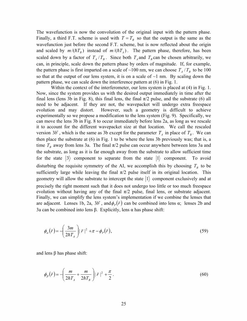
The wavefunction is now the convolution of the original input with the pattern phase. Finally, a third F.T. scheme is used with T BT= so that the output is the same as the wavefunction just before the second F.T. scheme, but is now reflected about the origin and scaled by m instead of . The pattern phase, therefore, has been scaled down by a factor of T . Since both T and can be chosen arbitrarily, we can, in principle, scale down the pattern phase by orders of magnitude. If, for example, the pattern phase is first imparted on a scale of ~100 nm, we can choose T to be 100 so that at the output of our lens system, it is on a scale of ~1 nm. By scaling down the pattern phase, we can scale down the interference pattern at (6) in Fig. 1.

)/( BTh )AT/(m h

BA T/ A BT

BA T/

B

3

1

b′ ( )rPvφ

)rTm

A

v

h

||

23

Pφπ −

2π|| 2 +

rv

22+

Tm

A hh

Within the context of the interferometer, our lens system is placed at (4) in Fig. 1. Now, since the system provides us with the desired output immediately in time after the final lens (lens 3b in Fig. 8), this final lens, the final π/2 pulse, and the substrate (6) all need to be adjacent. If they are not, the wavepacket will undergo extra freespace evolution and may distort. However, such a geometry is difficult to achieve experimentally so we propose a modification to the lens system (Fig. 9). Specifically, we can move the lens 3b in Fig. 8 to occur immediately before lens 2a, as long as we rescale it to account for the different wavepacket size at that location. We call the rescaled version 3 , which is the same as 3b except for the parameter T in place of T . We can then place the substrate at (6) in Fig. 1 to be where the lens 3b previously was; that is, a time T away from lens 3a. The final π/2 pulse can occur anywhere between lens 3a and the substrate, as long as it is far enough away from the substrate to allow sufficient time for the state

b′ A

B

component to separate from the state 1 component. To avoid disturbing the requisite symmetry of the AI, we accomplish this by choosing T to be sufficiently large while leaving the final π/2 pulse itself in its original location. This geometry will allow the substrate to intercept the state

B

component exclusively and at precisely the right moment such that it does not undergo too little or too much freespace evolution without having any of the final π/2 pulse, final lens, or substrate adjacent. Finally, we can simplify the lens system’s implementation if we combine the lenses that are adjacent. Lenses 1b, 2a, 3 , and can be combined into lens α; lenses 2b and 3a can be combined into lens β. Explicitly, lens α has phase shift:

( ) (rr vvφα +

−= 2 , (59)

and lens β has phase shift:

( )φβ

−=

Tmr

B

v . (60)

25

Fig. 10 shows the implementation of the lens system within the context of the whole AI. The reader may have a cause for concern in the fact that with the lens system in place, the part of the wavepacket that travels along the arm without the lens will be interfering not with a phase modified version of itself, but with a phase modified Fourier transform of itself. That is, the output of the lens system is a phase modified Fourier transform of its input. As such, the effective width of the wavepacket coming from the lens system may be significantly larger than the effective width of that coming from the arm without lenses, thus causing a truncation of the pattern formation around the edges. This problem is addressed by selecting T such that the wavepacket from the lens system is scaled to have an effective width equivalent to or smaller than the wavepacket from the other arm. Also, because of the Fourier transform, the wavepacket coming from the lens system, even without an added pattern phase, may have a different phase signature than the wavepacket coming from the other arm. Regarding this issue, our numerical experiments show that after freespace propagation for a time on the order of the timescale determined as practical (see section on practical considerations), the phase difference between the original wavepacket and its Fourier transform is very small over the span of the effective width of the wavepacket. Thus, the effect of this phase noise on the interference pattern is negligible.

B

IV. Some Practical Considerations IV. A. Wavepacket Behavior

The behavior of the wavepacket primarily has implications for the time and wavepacket effective width parameters of the lithography scheme. As mentioned earlier, the scale limit of the intensity variation that creates the pattern phase when it is first applied is meters. The lens system then further reduces the scale of the pattern phase by a factor of T . To achieve lithography features on the scale of ~1nm, this ratio needs to be ~100. However, we must also take into consideration the extent of the entire intensity variation. In other words, referring to Fig. 10, the effective width of the wavepacket at lens α must be large enough to accommodate the entire pattern on the light pulse bearing the phase pattern information. We assume that this dimension will be on the order of a millimeter. We know that the wavepacket at lens α is a scaled Fourier transform of the wavepacket immediately before lens 1a, so that its effective width at lens

α is

710~BA T/

in

A

mTσh

~≤A

. This must be on the order of 10 . Also, another way in which the time

parameters are restricted is by the total amount of time that the atom spends in the AI. Even with a magnetic field slowing the atom’s fall, it is not practical to have the atom spend a large amount of time in the chamber. We therefore impose the restriction that the atom spend no more time than a minute or two in the chamber. Explicitly, this translates to: T .

3−

110

26

Now, as shown earlier, it is the state 1 component in our scheme that will form the desired interference pattern. The substrate must therefore intercept this component exclusive of the state 3 component. Fortunately, the state 3 component will have an additional velocity in the y direction due to photon recoil so that the two states will separate if given enough time. Also recall that each wavepacket state after the final π/2 pulse is composed of two elements, one that went through the lens system and one that did not, such that the elements that traveled along the arm without the lens system will have larger effective widths (since the output of the lens system is smaller than its input). The two states will be sufficiently separated, then, when the state 3 component has traveled far enough in the +y direction after the final π/2 pulse such that there is no overlap of the larger effective widths. Since we know that photon recoil gives the state 3 component an additional momentum of 2 in the +y direction, we have: mv = 2

Also, it can be shown that the effective width of a wavepacket after passing through freespace for a time T is

kh .kh

( )τσ /1 T+ , where h/στ m= and σ is the original effective width. Therefore, for sufficient spatial separation of the states (assuming that the time between the final π/2 pulse and the substrate is on the order of T ) we need: v

B

( )τσ /1~ BinB TT +≥* . To summarize, our restrictions are:

110~≤AT AB TT 210~ −≤ 310~ −≥in

A

mTσh

+≥

in

BinB m

TTm

kσ

σhh 1~2 .

After using some simple algebra, we find that the first three restrictions are satisfied if we apply the following:

510−≤inσ 16 10~10~ ≤≤ Ain Tσ AB TT 210~ −≤ . We can, for example, choose: , , . A simple check shows that these choices also satisfy the fourth restriction.

510−=inσ 110~AT 110~ −BT

Finally, since our proposed lithography scheme involves the use of a single atom at a time, it entails the drawback of being very slow. To make this type of lithography truly practical, a Bose-Einstein condensate would have to be used instead of a single atomic wavepacket. The analysis for using BEC - ] is the next area of research. [4 [6 IV. B. Rubidium 87 Transition Scheme For practical implementation of our three-level atom, we use the D1 transitions in rubidium 87 ]. Fig. 11 illustrates. One of the restrictions is that, in order to be able to neglect spontaneous emission, we need for each single transition:

[36

27

1**2

0 <<Γ

τδg

, (61)

where is the Rabi frequency, δ is the detuning, Γ is the decay rate, and τ is the interaction time. Both the Raman pulse scheme and the light shift scheme also require:

0g

δ<<0g . (62)

Each of the transitions that we have chosen are the strongest ones from their group, so we assume them both to have a saturation intensity of about . We have the following relation:

2/3 cmmW

2max2max,0

Γ

=

satII

g . (63)

If we assume and , we find that

Hz.

2max /2 mmWI = 17 sec10*33.3 −=Γ

9max,0 10*6.8≈g

Now, the polarized light that we have chosen excites not only the desired transition from

+σ1 to 2 , but also a transition from 2 to a different metastable state

which we do not wish to populate. Fortunately, this second transition is about 6.8 GHz less than the first one, and its coupling strength is about 4 times smaller. The π polarized light that we have chosen for the 2 to 3 transition also excites undesired transitions

by linking state 1 to excited states other than the one we have chosen for 2 . However, the undesired transitions that are excited in this case are also over 6 GHz larger than the desired transition. We can therefore neglect the unwanted transitions by making sure that our polarized and π polarized pulses are detuned from their appropriate transitions by no more than a few hundred MHz, thereby assuring that the detuning for the unwanted transitions is at least a factor of 10 greater than the detuning for the desired transitions. We choose our detuning to be 680 MHz.

+σ

In order to satisfy the constraint that the Rabi frequency be much less than the detuning, we choose 68 MHz. This is well below the maximum limit calculated above.

=0g

As far as the interaction time for the π/2 and π pulse scheme, it is the Raman Rabi frequency that is of interest:

28

δ2

20g

=Ω . (64)

Using this in Eq. (61), we get:

Γ<<Ω⇒

<<ΓΩ

2

1**2

δτ

τδ

(65)

Plugging in the chosen value for δ and the typical value of 33.33 MHz for Γ, we find that

2.10<<Ωτ . We can satisfy this restraint by choosing πτ =Ω for the π pulse and half as much for the π/2 pulse, giving a pulse duration of 924/ ≈Ω= πτ ns for a π pulse and

462≈τ ns for a π/2 pulse. For the light shift we use the same π polarized excitation of state 3 as above. The time constraint in this case is:

πτδ

24

20 =

g. (66)

This gives an interaction time of 7.3≈τ µsec. Ideally, the light shift pulse will only interact with the wavepacket in state 3

110~

. This may actually be possible if we choose T to be large enough such that the two states gain enough of a transverse separation. If, as by example above, we choose T , then the separation between the two states will be on the order of a centimeter and there will be virtually no overlap between the two components of the wavepacket in the separate arms. The light pulse could then simply intercept only state

A

A

3 . If, however, the situation is such that the states are overlapping,

then state 1 will also see the light shift, but it will be about a factor of 10 less because of

the detuning being approximately 10 times larger for it than for the state 3 transition. V. Numerical Experiments The numerical implementation of our lithography scheme was done in Matlab by distributing the wavepackets across finite meshes and then evolving them according to the Schrodinger equation. This evolution was done in both position and momentum space according to expediency. To go between the two domains, we used two-dimensional Fourier Transform and Inverse Fourier Transform algorithms.

29

The initial wavepacket was taken in momentum space and completely in internal state 1 . Specifically, the wavepacket was given by the Fourier Transform of Eq. (2):

( )

−==Φ

2exp0,

22σ

πσ k

tke

vv

. (67)

The evolution of the wavepackets in the π and 2/π pulses was done in momentum space in order to be able to account for the different detunings that result for each momentum component due to the Doppler shift. Specifically, we numerically solved Eq. (27) for the different components of the k-space wavepacket mesh, then applied the inverse of the transformation matrix given by Eq. (20) to go to the original basis.

Outside of the lens system, the freespace evolution of the wavepackets was also done in momentum space. This was achieved easily by using Eq. (11). Within the lens system, however, it was more computationally efficient to use Eq. (57) for the freespace evolution because of the need to apply the lenses in position space. The results of using Eq. (57) were initially cross-checked with the results of using Eq. (11) and were found to agree. Fig. 12 and 13 demonstrate the formation of an arbitrary pattern by interference of the state 1 wavepackets at the output of the interferometer. Both figures were the result of applying the same arbitrary pattern phase, but Fig. 12 was formed without any shrinking implemented (i.e. TA=TB). Fig. 13, however, demonstrates the shrinking ability of the lens system by yielding a version of Fig. 12 that is scaled by a factor of two ( 2=BA TT ). The length scales are in arbitrary units due to the use of naturalized units for the sake of computational viability. VI. Suggestions for Extension to BEC

As mentioned above, in order to make this lithography scheme truly practical, a Bose-Einstein condensate is required in place of the single atom. The difficulty in using the BEC, however, is that the nonlinear term in the Gross-Pitaevskii equation (GPE) that describes its behavior renders our lens system useless because the analysis for the lens system was done for the linear SE.

One approach to getting around this problem is to try to eliminate the nonlinear term. Specifically, the GPE for the BEC takes the form

Ψ

Ψ++∇

−=

∂Ψ∂ 2

02

2

2UV

mti hh , (68)

30

where the nonlinear term coefficient is U and a is the scattering length for the atom. It has been demonstrated for

ma /4 20 hπ=

87Rb that the scattering length can be tuned over a broad range by exposing the BEC to magnetic fields of varying strength near Feshbach resonances ]. The relationship between the scattering length and the applied magnetic field B when near a Feshbach resonance can be written as

[37[38

−∆

−=peak

bg BBaa 1 , (69)

where is the background scattering length, is the resonance position, and . Setting would therefore set the scattering length to zero and

eliminate the nonlinear term in the GPE. While the atom-atom interaction may not be completely eliminated in reality due to the fluctuation in density that we wish to effect through the lens system, it is worth investigating if it could be made to be negligible over an acceptable range. We could then use our previously developed lens system to perform the imaging and thereby interfere thousands or millions of atoms simultaneously.

bga

zero −peakB

peakBB=∆ zeroBB =

This work was supported by DARPA grant # F30602-01-2-0546 under the QUIST program, ARO grant # DAAD19-001-0177 under the MURI program, and NRO grant # NRO-000-00-C-0158.

31

References [1] P. Rai-Choudhury (Ed), Hand book of Micro-lithography, Micromachining and Microfabrication, SPIE Press (1979).

[2] James R. Sheats & Bruce W. Smith (Ed), Microlithography Science & Technology, Chapter 7 X-Ray Lithography.

[3] Joseph W. Goodman, Introduction To Fourier Optics, McGraw-Hill Science/Engineering/Math , 1996.

[4] M. R. Andrews, C. G. Townsend, H.-J. Miesner, D. S. Durfee, D. M. Kurn, W. Ketterle, Science 275, 637 (1997).

[5] Kasevich, M. A. (2002). Science 298: 1363-1368 [6] Yoshio Torii, Yoichi Suzuki, Mikio Kozuma, Takahiro Kuga, Lu Deng, E.W. Hagley,

Quantum Electronics and Laser Science Conference 1999, Postdeadline papers QPD12-1

[7] C.J. Borde, Phys. Lett. A 140 (10), 1989. [8] M. Kasevich and S. Chu, Phys. Rev. Lett. 67, 181-184 (1991). [9] L. Gustavson, P. Bouyer, and M. A. Kasevich, Phys. Rev. Lett. 78, 2046-2049 (1997) [10] M. J. Snadden, J. M. McGuirk, P. Bouyer, K. G. Haritos, and M. A. Kasevich, Phys. Rev.

Lett. 81, 971-974 (1998) [11] TJ. M. McGuirk, M. J. Snadden, and M. A. Kasevich, Phys. Rev. Lett. 85, 4498-4501

(2000). [12] Y. Tan, J. Morzinski, A.V. Turukhin, P.S. Bhatia, and M.S. Shahriar, “Two-Dimensional

Atomic Interferometry for Creation of Nanostructures,”to appear in Opt. Comm. [13] D. Keith, C.Ekstrom, Q. Turchette, and D.E. Pritchard, Phys. Rev. Lett. 66, 2693 (1991) [14] D.S. Weiss, B.C. Young, and S. Chu, Phys. Rev. Lett. 70, 2706 (1993). [15] T. Pfau et al., Phys. Rev. Lett. 71, 3427 (1993) [16] U. Janicke and M. Wilkens, Phys. Rev. A. 50, 3265 (1994). [17] R. Grimm, J. Soding, and Yu.B. Ovchinnikov, Opt. Lett. 19, 658(1994). [18] T. Pfau, C.S. Adams, and J. Mlynek, Europhys. Lett. 21, 439 (1993). [19] K. Johnson, A. Chu, T.W. Lynn, K. Berggren, M.S. Shahriar, and M.G. Prentiss,

“Demonstration of a nonmagnetic blazed-grating atomic beam splitter,” Opt. Lett. 20, (1995).

[20] M.S. Shahriar, Y. Tan, M. Jheeta, J. Morzinksy, and P.R. Hemmer, “Observation of Continuously Guided Atomic Interferometry Using a Single-Zone Optical Excitation,” submitted to Phys. Rev. Letts.

[21] B. E. A. Saleh and M.C. Teich, Fundamentals of Photonics, Wiley-Interscience (1991).

[22] P.M. Radmore and and P.L. Knight, J. Phys. B. 15, 3405 (1982) [23] M. Prentiss, N. Bigelow, M.S. Shahriar and P. Hemmer, Optics Letters, 16, 1695(1991). [24] P.R. Hemmer, M.S. Shahriar, M. Prentiss, D. Katz, K. Berggren, J. Mervis, and N.

Bigelow Phys. Rev. Lett. 68, 3148 (1992). [25] M.S. Shahriar and P. Hemmer, Physical Review Letters, 65, 1865(1990). [26] M.S. Shahriar, P. Hemmer, D.P. Katz, A. Lee and M. Prentiss, Phys. Rev. A. 55, 2272

(1997).

32

[27] P. Meystre, Atom Optics (Springer Verlag 2001). [28] P.Berman(ed.), Atom Interferometry (Academic Press, 1997) . [29] S. Ezekiel and A. Arditty (eds.), Fiber Optic Rotation Sensors (Springer-Verlag, 1982). [30] J. McKeever et al. , Phys. Rev. Lett. 90, 133602 (2003). [31] S. J. van Enk et al., Phys. Rev. A 64, 013407 (2001). [32] A. C. Doherty et al. , Phys. Rev. A 63, 013401 (2000). [33] Changsoon Kim, Max Shtein, and Stephen R. Forrest, Applied Physics Letters Vol

80(21) , 4051( 2002) [34] S.M. Sharriar etal , to be suibmitted to PRA [35] L. Allen and J. H. Eberly, Optical Resonance and two-level atoms, Dover

Publication, INC, NY, (1974) [36] A. Corney, Atomic and Laser Spectroscopy, Oxford Science Publication. (1976) [37] Thomas Volz, Stephan Dürr, Sebastian Ernst, Andreas Marte, and Gerhard Rempe

Phys. Rev. A 68, 010702(R) (2003) [38] A. Marte, T. Volz, J. Schuster, S. Dürr, G. Rempe, E. G. M. van Kempen, and B. J.

Verhaa, Phys. Rev. Lett. 89, 283202 (2002)

33

1. 2. 3b.

3a. 4.5.

6.

x y

z

FIG. 1. 1.) atom beam source, 2.) π/2 pulse, 3.) π pulse 4.) an introduced phase shift φ(x,y), 5.) π/2 pulse, 6.) substrate with incident beam intensity proportional to 1+cos(φ(x,y)). The lasers at 2, 3, and 5 propagate parallel to the y axis in the y-z plane, and the atom beam propagates in the y-z plane. The beam is split at 2. in to two equally populated sub-beams. At 5. the sub-beams are mixed so that each one is distributed between both of the forward trajectories. The substrate at 6 is in the x-y plane.

34

SAM-coatedWafer

( )yxP ,

( )yxP ,cos 1−

Atoms

FIG. 2. The overall scheme. The second half of the interferometer has been stretched beyond proportion for the sake of clarity. is the normalized pattern that is to be fabricated. The right-most drawing represents a simplified energy level diagram and the various light fields’ relation to it. Light green are the π and π/2 pulses, red are the lenses, and blue is the pattern phase mask. Purple indicates the lower ground state of the atom and dark green indicates the other ground state. The black curves in the interferometer denote the magnetic field.

( yxP , )

35

1

External Internal

x

z

y

z

2

3

FIG. 3. The model of the atom. Externally, the atom is modeled as a 2D Gaussisan wavepacket in the x and y directions. Internally, it is a three-level system in the Λ configuration and initially in state 1 .

36

x

( )xeΨ

( )xI

x

( )yI

( )yeΨy

y

(a)

(b)

(c)

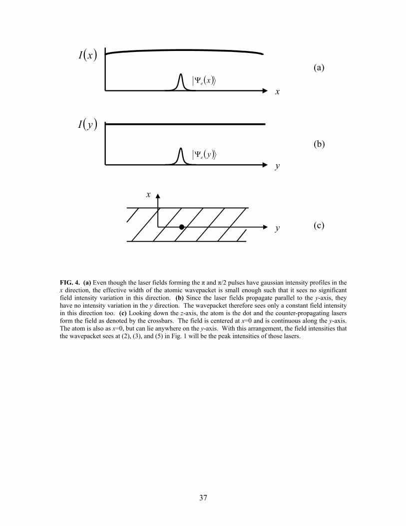
FIG. 4. (a) Even though the laser fields forming the π and π/2 pulses have gaussian intensity profiles in the x direction, the effective width of the atomic wavepacket is small enough such that it sees no significant field intensity variation in this direction. (b) Since the laser fields propagate parallel to the y-axis, they have no intensity variation in the y direction. The wavepacket therefore sees only a constant field intensity in this direction too. (c) Looking down the z-axis, the atom is the dot and the counter-propagating lasers form the field as denoted by the crossbars. The field is centered at x=0 and is continuous along the y-axis. The atom is also as x=0, but can lie anywhere on the y-axis. With this arrangement, the field intensities that the wavepacket sees at (2), (3), and (5) in Fig. 1 will be the peak intensities of those lasers.

37

0,1 p

( )BA kkp ++ h0,3

Akp h+0,2δh

BEv

AEv

AE

FIG. 5. One of the momentum manifolds within which the internal evolution takes place. For this particular momentum grouping, the lasers are detuned from their respective transitions by the same amount δ. The laser field that propagates in the +y direction,

v,

excites only the transition between states 1 and 2 . An atom going from state 1 to

state 2 AE will absorb a photon from v

and thereby gain momentum in the +y

direction. The laser that propagates in the opposite direction, Akh

BEv

, excites only the transition between states 3 and 2 . An atom going from state 2 to state 3

Bk BE

will emit

a photon with momentum h in the direction of v

and thereby gain an equivalent momentum in the direction of AE

v.

38

0I

δ4

20gh

δ4

20gh

−

δh−

0

0

Eige

nsta

te E

nerg

yLa

ser I

nten

sity

Position

FIG. 6. An illustration of the AC-Stark Effect. We see that the ground state, labeled here as W , has its energy linearly proportional to the laser’s intensity. As the intensity varies

with position, so does the energy of W . Note that this picture makes the assumption that the detuning δ is much larger than the square root of the peak intensity.

39

( ) ( )( )rPrI vv arccos∝

( )revΨ ( ) ( )ri

ePervv φ−Ψ

τ τ

x y

z

FIG. 7. The pattern phase is applied using a pulse of light traveling in the z direction that interacts with the wavepacket for a length of time τ and that has an intensity ( )rI v

in the transverse plane as shown. ( )rP v

is the arbitrary pattern and (rP )vφ is the corresponding pattern phase. (1) Before the interaction. (2) After the interaction; the wavepacket now carries the desired phase signature.

40

( )rvΨ

Φ r

Tm

A

v

h

−−

Φ

rTTi

A

B

AP

erTm

vv

h

φ

( )ri

A

PerTm vv

hφ−

Φ

TA TA TB

1a 1b 2a 3a2b 3b

t FIG. 8. The lens system. Each lens is actually a pulse of light with a transverse intensity modulation, much like the pulse in Fig. 7. Between lenses 1a and 1b and 2a and 2b are freespace regions of time duration , while between lenses 3a and 3b there is a freespace region of duration T . Lenses 1a and 2a

give the wavefunction a phase

AT B

221 2

rT

m

Aaa

v

h−== φφ , lenses 1b and 2b impart a phase

222

1 2πφφ +−= r

Tm

Ab

v

h=b , lens 3a gives a phase

23 2

rT

m

Ba

v

h−=φ , and lens 3b gives a phase

22

3 2πφ +−= r

TBb

vmh

.

41

( )rvΨ

−−

Φ

rTTi

A

B

AP

erTm

vv

h

φ

TA TA TB

1a 1b 2a 3a2b3b´

t FIG. 9. The lens system from Fig. 8 rearranged. The input and output are still the same, but the output is no longer immediately preceded by a lens. Lens b′3 is the same as lens 3b from Fig. 8 except for a T in

place of T so that it gives a phase shift of

A

B 22

'3 2πφ +r

Tm

Ab

v

h−= .

42

x y

z

1a α β

FIG. 10. The modified lens system in context. The π and π/2 pulses are not shown for the sake of simplicity. Lenses α and β are composites of the lenses from the system of Fig. 9. Between lenses 1a and α is a freespace region of time length T , as well as between lenses α and β . Between lens β and the

substrate is a freespace region of time duration T .

A

B ( ) ( )rrTmr P

A

vv

h

v φπφα −+

−= 2||

23

,

( )2

||22

2 πφβ +

+−= r

Tm

Tmr

BA

v

hh

v.

43

F=1-1 0 1

-2 -1 0 1 2

-2 -1 0 1 2F=2

F=2

87Rb D1-line

σ+

π

1

2

3

δ

6.8 GHz

680 MHz

FIG. 11. The transition scheme. σ+-polarized light excites the 21 ↔ transition and π-polarized light

excites the 32 ↔ transition. Both lasers are detuned by 680 MHz. For the π and π/2 pulses, the two transitions are simultaneously excited. For the light shift based lens system, only the π-polarized light is applied so as to affect only state 3 . The detuning of the lasers is small enough such that all other

transitions from the states 1 , 2 , and 3 that are excitable by either the σ+-polarized or π-polarized light see a detuning that is at least a factor of 10 larger. They can therefore be neglected.

44

FIG. 12. An arbitrary image is formed with the lens system in place, but without any scaling. We see that it is a more complex pattern than just a simple periodic structure such as sinusoidal fringes.

45

46

FIG. 13. The same image as in Fig. 12 is formed with the lens system still in place, but a scaling factor of two has been used to shrink the pattern. No distortion results from this scaling.