Tutorial on Exploratory Data Analysis eserved@d =...
48
Introduction Individuals cloud Variables cloud Helps to interpret Tutorial on Exploratory Data Analysis Julie Josse, François Husson, Sébastien Lê julie.josse at agrocampus-ouest.fr francois.husson at agrocampus-ouest.fr Applied Mathematics Department, Agrocampus Ouest useR-2008 Dortmund, August 11th 2008 1 / 48
Transcript of Tutorial on Exploratory Data Analysis eserved@d =...

Introduction Individuals cloud Variables cloud Helps to interpret
Tutorial on Exploratory DataAnalysis
Julie Josse, François Husson, Sébastien Lê
julie.josse at agrocampus-ouest.frfrancois.husson at agrocampus-ouest.fr
Applied Mathematics Department, Agrocampus Ouest
useR-2008Dortmund, August 11th 2008
1 / 48

Introduction Individuals cloud Variables cloud Helps to interpret
Why a tutorial on Exploratory Data Analysis?
• Our research focus on multi-table data analysis• We teach Exploratory Data analysis from a long time (but in
French ...)• We made an R package:
• Possibility to add supplementary information• The use of a more geometrical point of view allowing to draw
graphs• The possibility to propose new methods (taking into account
different structure on the data)• To have a package user friendly and oriented to practitioner (a
very easy GUI)
2 / 48
Introduction Individuals cloud Variables cloud Helps to interpret
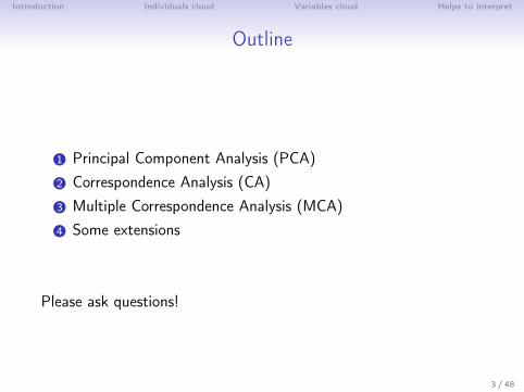
Outline
1 Principal Component Analysis (PCA)2 Correspondence Analysis (CA)3 Multiple Correspondence Analysis (MCA)4 Some extensions
Please ask questions!
3 / 48

Introduction Individuals cloud Variables cloud Helps to interpret
Multivariate data analysis
• Principal Component Analysis (PCA) ⇒ continuous variables• Correspondence Analysis (CA) ⇒ contingency table• Multiple Correspondence Analysis (MCA) ⇒ categorical
variables
• Dimensionality reduction ⇒ describe the dataset with smallernumber of variables
• Techniques widely used for applications such as: datacompression, data reconstruction; preprocessing beforeclustering, and ...
4 / 48

Introduction Individuals cloud Variables cloud Helps to interpret
Exploratory data analysis
⇒ Descriptive methods⇒ Data visualization⇒ Geometrical approach: importance to graphical outputs⇒ Identification of clusters, detection of outliers
⇒ French school (Benzécri)
5 / 48

Introduction Individuals cloud Variables cloud Helps to interpret
Principal Component Analysis
6 / 48

Introduction Individuals cloud Variables cloud Helps to interpret
PCA in R
• prcomp, princomp from stats• dudi.pca from ade4 (http://pbil.univ-lyon1.fr/ADE-4)• PCA from FactoMineR (http://factominer.free.fr)
7 / 48

Introduction Individuals cloud Variables cloud Helps to interpret
PCA deals with which kind of data?
Figure: Data table in PCA.
Notations:
xi . the individual i ,S = 1
nX ′cXc the covariance
matrix,W = XcX ′
c the inner productsmatrix.
• PCA deals with continuous variables, but categorical variablescan also be included in the analysis
8 / 48

Introduction Individuals cloud Variables cloud Helps to interpret
Some examples
• Many examples• Sensory analysis: products - descriptors• Environmental data: plants - measurements; waters -
physico-chemical analyses• Economy: countries - economic indicators• Microbiology: cheeses - microbiological analyses• etc.
• Today we illustrate PCA with:• data decathlon: athletes performances during two athletics
meetings• data chicken: genomics data
9 / 48

Introduction Individuals cloud Variables cloud Helps to interpret
Decathlon data• 41 athletes (rows)• 13 variables (columns):
• 10 continuous variables corresponding to the performances• 2 continuous variables corresponding to the rank and the
points obtained• 1 categorical variable corresponding to the athletics meeting:
Olympic Game and Decastar (2004)
Data : performances of 41 athletes during two meetings of decathlon
100
m
Lo
ng
.jum
p
Sh
ot.
pu
t
Hig
h.ju
mp
40
0m
110
m.h
urd
le
Dis
cu
s
Po
le.v
ault
Jav
elin
e
150
0m
Ra
nk
Po
ints
Co
mp
eti
tio
n
SEBRLE 11.04 7.58 14.83 2.07 49.81 14.69 43.75 5.02 63.19 291.70 1 8217 Decastar CLAY 10.76 7.40 14.26 1.86 49.37 14.05 50.72 4.92 60.15 301.50 2 8122 Decastar KARPOV 11.02 7.30 14.77 2.04 48.37 14.09 48.95 4.92 50.31 300.20 3 8099 Decastar BERNARD 11.02 7.23 14.25 1.92 48.93 14.99 40.87 5.32 62.77 280.10 4 8067 Decastar YURKOV 11.34 7.09 15.19 2.10 50.42 15.31 46.26 4.72 63.44 276.40 5 8036 Decastar Sebrle 10.85 7.84 16.36 2.12 48.36 14.05 48.72 5.00 70.52 280.01 1 8893 OlympicG Clay 10.44 7.96 15.23 2.06 49.19 14.13 50.11 4.90 69.71 282.00 2 8820 OlympicG Karpov 10.50 7.81 15.93 2.09 46.81 13.97 51.65 4.60 55.54 278.11 3 8725 OlympicG Macey 10.89 7.47 15.73 2.15 48.97 14.56 48.34 4.40 58.46 265.42 4 8414 OlympicG Warners 10.62 7.74 14.48 1.97 47.97 14.01 43.73 4.90 55.39 278.05 5 8343 OlympicG
PCA Example
10 / 48

Introduction Individuals cloud Variables cloud Helps to interpret
Problems - objectives
• Individuals study: similarity between individuals for all thevariables (Euclidian distance) → partition between individuals
• Variables study: are there linear relationships betweenvariables? Visualization of the correlation matrix; find somesynthetic variables
• Link between the two studies: characterization of the groupsof individuals by the variables; particular individuals to betterunderstand the links between variables
11 / 48
Introduction Individuals cloud Variables cloud Helps to interpret
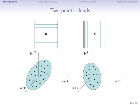
Two points clouds
XX
var 1
var k
ind 1
ind k
12 / 48

Introduction Individuals cloud Variables cloud Helps to interpret
Pre-processing: Mean centering, Scaling?• Mean centering does not modify the shape of the cloud• Scaling: variables are always scaled when they are not in the
same units
+ ++++ ++ ++ +++ ++ +++ +++ +++ +++ ++ ++ + + + ++ ++ + ++ +
−10 0 10 20 30 40
−20
−10
010
20
Time for 1500 m (s)
Long
jum
p (in
m)
+
+
+
+
+
+
+ +
+
+
+
+
+
+
+
+
+
+
++
+++
++
+
+
+
+
+
++
+
+
+
+
+
+
+
+
+
−50 0 50
−60
−40
−20
020
4060
Time for 1500 m (s)
Long
jum
p (in
cm
)
⇒ PCA always centered and often scaled13 / 48

Introduction Individuals cloud Variables cloud Helps to interpret
Individuals cloud
• Individuals are in RK
• Similarity between individuals: Euclidean distance• Study the structure, i.e. the shape of the individual cloud
14 / 48

Introduction Individuals cloud Variables cloud Helps to interpret
Inertia
• Total inertia ⇒ multidimensional variance ⇒ distance betweenthe data and the barycenter:
Ig =I∑
i=1
pi ||xi . − g ||2 =1I
I∑i=1
(xi . − g)′(xi . − g),
= tr(S) =∑
s
λs = K .
15 / 48

Introduction Individuals cloud Variables cloud Helps to interpret
Fit the individuals cloudFind the subspace who better sum up the data: the closest one byprojection.
Figure: Camel vs dromedary?
16 / 48
Introduction Individuals cloud Variables cloud Helps to interpret
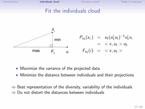
Fit the individuals cloud
xi.
Fu u
min
max
Pu1(xi .) = u1(u′1u1)−1u′1xi .
= < x , u1 > u1
Fu1(i) = < x , u1 >
• Maximize the variance of the projected data• Minimize the distance between individuals and their projections
⇒ Best representation of the diversity, variability of the individuals⇒ Do not distort the distances between individuals
17 / 48

Introduction Individuals cloud Variables cloud Helps to interpret
Find the subspace (1)• Find the first axis u1, for which variance of Fu1 = Xu1 is
maximized:
u1 = argmaxu1var(Xu1) with u′1u1 = 1
var(Fu1) =1I(Xu1)
′Xu1 = u′11IX ′Xu1
It leads to:
max u′1Su1 with u′1u1 = 1
⇒ u1 first eigenvector of S (associated with the largesteigenvalue λ1):
Su1 = λ1u1.
⇒ This eigenvector is known as the first axis (loadings).18 / 48

Introduction Individuals cloud Variables cloud Helps to interpret
Find the subspace (2)
⇒ Projected inertia on the first axis:
var(Fu1) = var(Xu1) = λ1
⇒ Percentage of variance explained by the first axis:
λ1∑k λk
• Additional axes are defined in an incremental fashion: each newdirection is chosen by maximizing the projected variance among allorthogonal directions
• Solution: K eigenvectors u1,...,uK of the data covariance matrixcorresponding to the K largest eigenvalues λ1,...,λK
19 / 48

Introduction Individuals cloud Variables cloud Helps to interpret
Example: graph of the individuals
●
−4 −2 0 2 4
−4
−2
02
4
Individuals factor map (PCA)
Dimension 1 (32.72%)
Dim
ensi
on 2
(17
.37%
)
●
●●
●
●
●
●
●
●●
●
●
●
●
●
●
●
●
●
●
●
●
●
●
●
●
●
●
●
●
●
●
●
●
●
●
●
●
●
●
●
SEBRLECLAYKARPOV
BERNARD
YURKOV
WARNERS
ZSIVOCZKY
McMULLENMARTINEAUHERNU
BARRAS
NOOL
BOURGUIGNON
Sebrle
Clay
Karpov
Macey
Warners
Zsivoczky
Hernu
Nool
Bernard
Schwarzl
Pogorelov
Schoenbeck
Barras
Smith
Averyanov
OjaniemiSmirnov
Qi
Drews
Parkhomenko
Terek
Gomez
Turi
Lorenzo
Karlivans
Korkizoglou
Uldal
Casarsa
⇒ Need variables to interpret the dimension of variability20 / 48
Introduction Individuals cloud Variables cloud Helps to interpret
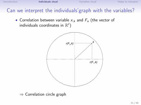
Can we interpret the individuals’graph with the variables?
• Correlation between variable x.k and Fu (the vector ofindividuals coordinates in RI )
r(F1,k)
r(F2,k)k
⇒ Correlation circle graph
21 / 48
Introduction Individuals cloud Variables cloud Helps to interpret
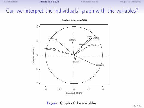
Can we interpret the individuals’ graph with the variables?
●
−1.0 −0.5 0.0 0.5 1.0
−1.
0−
0.5
0.0
0.5
1.0
Variables factor map (PCA)
Dimension 1 (32.72%)
Dim
ensi
on 2
(17
.37%
)
X100m
Long.jump
Shot.put
High.jump
X400m
X110m.hurdle
Discus
Pole.vault
Javeline
X1500m
Figure: Graph of the variables.22 / 48
Introduction Individuals cloud Variables cloud Helps to interpret
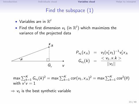
Find the subspace (1)
• Variables are in RI
• Find the first dimension v1 (in RI ) which maximizes thevariance of the projected data
x.k
Gv v
Pv1(x.k) = v1(v ′1v1)−1v ′1x.k
Gv1(k) =< v1, x .k >
||v1||
max∑K
k=1 Gv1(k)2 = max∑K
k=1 cor(v1, x.k)2 = max∑K
k=1 cos2(θ)with v ′v = 1
⇒ v1 is the best synthetic variable
23 / 48
Introduction Individuals cloud Variables cloud Helps to interpret
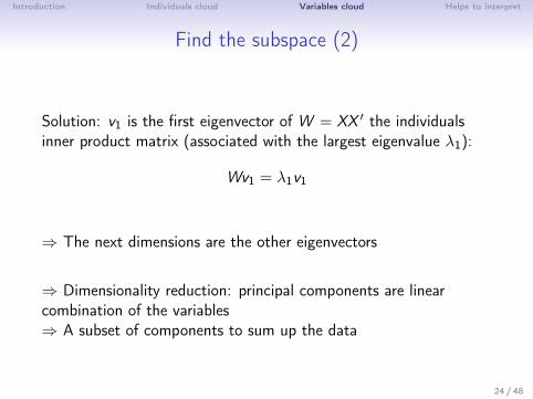
Find the subspace (2)
Solution: v1 is the first eigenvector of W = XX ′ the individualsinner product matrix (associated with the largest eigenvalue λ1):
Wv1 = λ1v1
⇒ The next dimensions are the other eigenvectors
⇒ Dimensionality reduction: principal components are linearcombination of the variables⇒ A subset of components to sum up the data
24 / 48

Introduction Individuals cloud Variables cloud Helps to interpret
Fit the variables cloud
●
−1.0 −0.5 0.0 0.5 1.0
−1.
0−
0.5
0.0
0.5
1.0
Variables factor map (PCA)
Dimension 1 (32.72%)
Dim
ensi
on 2
(17
.37%
)
X100m
Long.jump
Shot.put
High.jump
X400m
X110m.hurdle
Discus
Pole.vault
Javeline
X1500m
Figure: Graph of the variables.
⇒ Same representation! What a wonderful result!25 / 48

Introduction Individuals cloud Variables cloud Helps to interpret
Projections...
Only well projected variables (high cos2 between the variable andits projection) can be interpreted!
A
B
C
DHAHB
HCHD
HA
HB
HC
HD
26 / 48

Introduction Individuals cloud Variables cloud Helps to interpret
Exercices...
• With 200 independent variables and 7 individuals, how doesyour correlation circle look like?
27 / 48

Introduction Individuals cloud Variables cloud Helps to interpret
Exercices...
• With 200 independent variables and 7 individuals, how doesyour correlation circle look like?
mat=matrix(rnorm(7*200,0,1),ncol=200)PCA(mat)
28 / 48

Introduction Individuals cloud Variables cloud Helps to interpret
Link between the two representations: transition formulae
• Su = X ′Xu = λu• XX ′Xu = Xλu → W (Xu) = λ(Xu)
• WFu = λFu and since Wv = λv then Fu and v are colinear• Since, ||Fu|| = λ and ||v || = 1 we have:
v = 1√λFu ⇒ Gv = X ′v = 1√
λX ′Fu
u = 1√λGv ⇒ Fu = Xu = 1√
λXGv
Fs(i) =1√λs
K∑k=1
xikGs(k) Gs(k) =1√λs
I∑i=1
xikFs(i)
29 / 48
Introduction Individuals cloud Variables cloud Helps to interpret
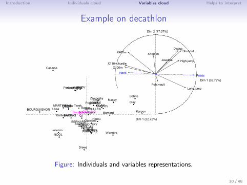
Example on decathlon
Dim 1 (32.72%)
Dim 2 (17.37%)
X100m
Long.jump
Shot.put
High.jump
X400m
X110m.hurdle
Discus
Pole.vault
Javeline
X1500m
RankPoints
Dim 1 (32.72%)
SEBRLECLAYKARPOV
BERNARD
YURKOV
WARNERS
ZSIVOCZKY
McMULLENMARTINEAUHERNU
BARRAS
NOOL
BOURGUIGNON
Sebrle
Clay
Karpov
Macey
Warners
Zsivoczky
Hernu
Nool
Bernard
Schwarzl
Pogorelov
Schoenbeck
Barras
Smith
Averyanov
OjaniemiSmirnov
Qi
Drews
Parkhomenko
Terek
Gomez
Turi
Lorenzo
Karlivans
Korkizoglou
Uldal
Casarsa
DecastarOlympicG
Figure: Individuals and variables representations.
30 / 48

Introduction Individuals cloud Variables cloud Helps to interpret
Supplementary information (1)• For the continuous variables: projection of these
supplementary variables on the dimensions
●
−1.0 −0.5 0.0 0.5 1.0
−1.
0−
0.5
0.0
0.5
1.0
Variables factor map (PCA)
Dimension 1 (32.72%)
Dim
ensi
on 2
(17
.37%
)
X100m
Long.jump
Shot.put
High.jump
X400m
X110m.hurdle
Discus
Pole.vault
Javeline
X1500m
RankPoints
• For the individuals: projection⇒ Supplementary information do not participate to create the axes
31 / 48

Introduction Individuals cloud Variables cloud Helps to interpret
Supplementary information (2)→ How to deal with (supplementary) categorical variables?
X100m Long.jump Shot.put High.jump CompetitionHERNU 11.37 7.56 14.41 1.86 DecastarBARRAS 11.33 6.97 14.09 1.95 DecastarNOOL 11.33 7.27 12.68 1.98 DecastarBOURGUIGNON 11.36 6.80 13.46 1.86 DecastarSebrle 10.85 7.84 16.36 2.12 OlympicGClay 10.44 7.96 15.23 2.06 OlympicG
X100m Long.jump Shot.put High.jumpHERNU 11.37 7.56 14.41 1.86BARRAS 11.33 6.97 14.09 1.95NOOL 11.33 7.27 12.68 1.98BOURGUIGNON 11.36 6.80 13.46 1.86Sebrle 10.85 7.84 16.36 2.12Clay 10.44 7.96 15.23 2.06
Decastar 11.18 7.25 14.16 1.98 Olympic.G 10.92 7.27 14.62 1.98
→ The categories are projected at the barycenter of the individualswho take the categories 32 / 48

Introduction Individuals cloud Variables cloud Helps to interpret
Supplementary information (3)
●
−4 −2 0 2 4
−4
−2
02
4
Individuals factor map (PCA)
Dimension 1 (32.72%)
Dim
ensi
on 2
(17
.37%
)
●
●●
●
●
●
●
●
●●
●
●
●
●
●
●
●
●
●
●
●
●
●
●
●
●
●
●
●
●
●
●
●
●
●
●
●
●
●
●
●
SEBRLECLAYKARPOV
BERNARD
YURKOV
WARNERS
ZSIVOCZKY
McMULLENMARTINEAUHERNU
BARRAS
NOOL
BOURGUIGNON
Sebrle
Clay
Karpov
Macey
Warners
Zsivoczky
Hernu
Nool
Bernard
Schwarzl
Pogorelov
Schoenbeck
Barras
Smith
Averyanov
OjaniemiSmirnov
Qi
Drews
Parkhomenko
Terek
Gomez
Turi
Lorenzo
Karlivans
Korkizoglou
Uldal
Casarsa
DecastarOlympicG
DecastarOlympicG
Figure: Projection of supplementary variables.
33 / 48

Introduction Individuals cloud Variables cloud Helps to interpret
Confidence ellipses
●
−4 −2 0 2 4
−4
−2
02
4
Individuals factor map (PCA)
Dimension 1 (32.72%)
Dim
ensi
on 2
(17
.37%
)
●
●●
●
●
●
●
●
●●
●
●
●
●
●
●
●
●
●
●
●
●
●
●
●
●
●
●
●
●
●
●
●
●
●
●
●
●
●
●
●
SEBRLECLAYKARPOV
BERNARD
YURKOV
WARNERS
ZSIVOCZKY
McMULLENMARTINEAUHERNU
BARRAS
NOOL
BOURGUIGNON
Sebrle
Clay
Karpov
Macey
Warners
Zsivoczky
Hernu
Nool
Bernard
Schwarzl
Pogorelov
Schoenbeck
Barras
Smith
Averyanov
OjaniemiSmirnov
Qi
Drews
Parkhomenko
Terek
Gomez
Turi
Lorenzo
Karlivans
Korkizoglou
Uldal
Casarsa
DecastarOlympicG
DecastarOlympicG
Figure: Confidence ellipses around the barycenter of each category.
34 / 48

Introduction Individuals cloud Variables cloud Helps to interpret
Number of dimensions?
• Percentage of variance explained by each axis: informationbrought by the dimension
• Quality of the approximation:∑Q
s λs∑Ks λs
• Dimensionality Reduction implies Information Loss
• Number of components to retain? Retain much of thevariability in our data (the other components are noise)
• Bar plot of the eigenvalues: scree test• Test on eigenvalues, confidence interval,...
35 / 48
Introduction Individuals cloud Variables cloud Helps to interpret
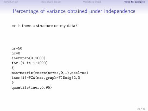
Percentage of variance obtained under independence
⇒ Is there a structure on my data?
nr=50nc=8iner=rep(0,1000)for (i in 1:1000){mat=matrix(rnorm(nr*nc,0,1),ncol=nc)iner[i]=PCA(mat,graph=F)$eig[2,3]}quantile(iner,0.95)
36 / 48

Introduction Individuals cloud Variables cloud Helps to interpret
Percentage of variance obtained under independence⇒ Is there a structure on my data?
Number of variablesnbind 4 5 6 7 8 9 10 11 12 13 14 15 16
5 96.5 93.1 90.2 87.6 85.5 83.4 81.9 80.7 79.4 78.1 77.4 76.6 75.56 93.3 88.6 84.8 81.5 79.1 76.9 75.1 73.2 72.2 70.8 69.8 68.7 68.07 90.5 84.9 80.9 77.4 74.4 72.0 70.1 68.3 67.0 65.3 64.3 63.2 62.28 88.1 82.3 77.2 73.8 70.7 68.2 66.1 64.0 62.8 61.2 60.0 59.0 58.09 86.1 79.5 74.8 70.7 67.4 65.1 62.9 61.1 59.4 57.9 56.5 55.4 54.310 84.5 77.5 72.3 68.2 65.0 62.4 60.1 58.3 56.5 55.1 53.7 52.5 51.511 82.8 75.7 70.3 66.3 62.9 60.1 58.0 56.0 54.4 52.7 51.3 50.1 49.212 81.5 74.0 68.6 64.4 61.2 58.3 55.8 54.0 52.4 50.9 49.3 48.2 47.213 80.0 72.5 67.2 62.9 59.4 56.7 54.4 52.2 50.5 48.9 47.7 46.6 45.414 79.0 71.5 65.7 61.5 58.1 55.1 52.8 50.8 49.0 47.5 46.2 45.0 44.015 78.1 70.3 64.6 60.3 57.0 53.9 51.5 49.4 47.8 46.1 44.9 43.6 42.516 77.3 69.4 63.5 59.2 55.6 52.9 50.3 48.3 46.6 45.2 43.6 42.4 41.417 76.5 68.4 62.6 58.2 54.7 51.8 49.3 47.1 45.5 44.0 42.6 41.4 40.318 75.5 67.6 61.8 57.1 53.7 50.8 48.4 46.3 44.6 43.0 41.6 40.4 39.319 75.1 67.0 60.9 56.5 52.8 49.9 47.4 45.5 43.7 42.1 40.7 39.6 38.420 74.1 66.1 60.1 55.6 52.1 49.1 46.6 44.7 42.9 41.3 39.8 38.7 37.525 72.0 63.3 57.1 52.5 48.9 46.0 43.4 41.4 39.6 38.1 36.7 35.5 34.530 69.8 61.1 55.1 50.3 46.7 43.6 41.1 39.1 37.3 35.7 34.4 33.2 32.135 68.5 59.6 53.3 48.6 44.9 41.9 39.5 37.4 35.6 34.0 32.7 31.6 30.440 67.5 58.3 52.0 47.3 43.4 40.5 38.0 36.0 34.1 32.7 31.3 30.1 29.145 66.4 57.1 50.8 46.1 42.4 39.3 36.9 34.8 33.1 31.5 30.2 29.0 27.950 65.6 56.3 49.9 45.2 41.4 38.4 35.9 33.9 32.1 30.5 29.2 28.1 27.0100 60.9 51.4 44.9 40.0 36.3 33.3 31.0 28.9 27.2 25.8 24.5 23.3 22.3
Table: 95 % quantile inertia on the two first dimensions of 10000 PCAon data with independent variables
37 / 48

Introduction Individuals cloud Variables cloud Helps to interpret
Percentage of variance obtained under independenceNumber of variables
nbind 17 18 19 20 25 30 35 40 50 75 100 150 2005 74.9 74.2 73.5 72.8 70.7 68.8 67.4 66.4 64.7 62.0 60.5 58.5 57.46 67.0 66.3 65.6 64.9 62.3 60.4 58.9 57.6 55.8 52.9 51.0 49.0 47.87 61.3 60.7 59.7 59.1 56.4 54.3 52.6 51.4 49.5 46.4 44.6 42.4 41.28 57.0 56.2 55.4 54.5 51.8 49.7 47.8 46.7 44.6 41.6 39.8 37.6 36.49 53.6 52.5 51.8 51.2 48.1 45.9 44.4 42.9 41.0 38.0 36.1 34.0 32.710 50.6 49.8 49.0 48.3 45.2 42.9 41.4 40.1 38.0 35.0 33.2 31.0 29.811 48.1 47.2 46.5 45.8 42.8 40.6 39.0 37.7 35.6 32.6 30.8 28.7 27.512 46.2 45.2 44.4 43.8 40.7 38.5 36.9 35.5 33.5 30.5 28.8 26.7 25.513 44.4 43.4 42.8 41.9 39.0 36.8 35.1 33.9 31.8 28.8 27.1 25.0 23.914 42.9 42.0 41.3 40.4 37.4 35.2 33.6 32.3 30.4 27.4 25.7 23.6 22.415 41.6 40.7 39.8 39.1 36.2 34.0 32.4 31.1 29.0 26.0 24.3 22.4 21.216 40.4 39.5 38.7 37.9 35.0 32.8 31.1 29.8 27.9 24.9 23.2 21.2 20.117 39.4 38.5 37.6 36.9 33.8 31.7 30.1 28.8 26.8 23.9 22.2 20.3 19.218 38.3 37.4 36.7 35.8 32.9 30.7 29.1 27.8 25.9 22.9 21.3 19.4 18.319 37.4 36.5 35.8 34.9 32.0 29.9 28.3 27.0 25.1 22.2 20.5 18.6 17.520 36.7 35.8 34.9 34.2 31.3 29.1 27.5 26.2 24.3 21.4 19.8 18.0 16.925 33.5 32.5 31.8 31.1 28.1 26.0 24.5 23.3 21.4 18.6 17.0 15.2 14.230 31.2 30.3 29.5 28.8 26.0 23.9 22.3 21.1 19.3 16.6 15.1 13.4 12.535 29.5 28.6 27.9 27.1 24.3 22.2 20.7 19.6 17.8 15.2 13.7 12.1 11.140 28.1 27.3 26.5 25.8 23.0 21.0 19.5 18.4 16.6 14.1 12.7 11.1 10.245 27.0 26.1 25.4 24.7 21.9 20.0 18.5 17.4 15.7 13.2 11.8 10.3 9.450 26.1 25.3 24.6 23.8 21.1 19.1 17.7 16.6 14.9 12.5 11.1 9.6 8.7100 21.5 20.7 19.9 19.3 16.7 14.9 13.6 12.5 11.0 8.9 7.7 6.4 5.7
Table: 95 % quantile inertia on the two first dimensions of 10000 PCAon data with independent variables
38 / 48

Introduction Individuals cloud Variables cloud Helps to interpret
Quality of the representation: cos2
• For the variables: only well projected variables (high cos2
between the variable and its projection) can be interpreted!
• For the individuals: (same idea) distance between individualscan only be interpreted for well projected individualsres.pca$ind$cos
Dim.1 Dim.2Sebrle 0.70 0.08Clay 0.71 0.03Karpov 0.85 0.00
39 / 48

Introduction Individuals cloud Variables cloud Helps to interpret
Contribution⇒ Contribution to the inertia to create the axis:
• For the individuals: Ctrs(i) = F 2s (i)∑I
i=1 F 2s (i)
= F 2s (i)λs
⇒ Individuals with large coordinate contribute the most to theconstruction of the axis
round(res.pca$ind$contrib,2)Dim.1 Dim.2
Sebrle 12.16 2.62Clay 11.45 0.98Karpov 15.91 0.00
• For the variables: Ctrs(k) =G2
s (k)λs
= cor(x.k ,vs )2
λs
⇒ Variables highly correlated with the principal componentcontribute the most to the construction of the dimension
40 / 48

Introduction Individuals cloud Variables cloud Helps to interpret
Description of the dimensions (1)By the quantitative variables:• The correlation between each variable and the coordinate of
the individuals (principal components) on the axis s iscalculated
• The correlation coefficients are sorted and significant ones aregiven
$Dim.1 $Dim.2$Dim.1$quanti $Dim.2$quantiDim.1 Dim.2Points 0.96 Discus 0.61Long.jump 0.74 Shot.put 0.60Shot.put 0.62Rank -0.67400m -0.68110m.hurdle -0.75100m -0.77
41 / 48
Introduction Individuals cloud Variables cloud Helps to interpret
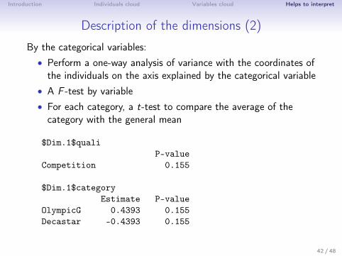
Description of the dimensions (2)
By the categorical variables:• Perform a one-way analysis of variance with the coordinates of
the individuals on the axis explained by the categorical variable• A F -test by variable• For each category, a t-test to compare the average of the
category with the general mean
$Dim.1$qualiP-value
Competition 0.155
$Dim.1$categoryEstimate P-value
OlympicG 0.4393 0.155Decastar -0.4393 0.155
42 / 48

Introduction Individuals cloud Variables cloud Helps to interpret
Practice
library(FactoMineR)data(decathlon)res <- PCA(decathlon,quanti.sup=11:12,quali.sup=13)plot(res,habillage=13)res$eigx11()barplot(res$eig[,1],main="Eigenvalues",names.arg=1:nrow(res$eig))res$ind$coordres$ind$cos2res$ind$contribdimdesc(res)aa=cbind.data.frame(decathlon[,13],res$ind$coord)bb=coord.ellipse(aa,bary=TRUE)plot.PCA(res,habillage=13,ellipse=bb)#write.infile(res,file="my_FactoMineR_results.csv") #to export a list
43 / 48
Introduction Individuals cloud Variables cloud Helps to interpret
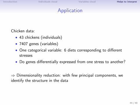
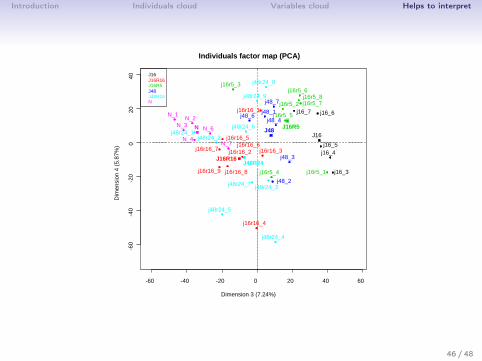
Application
Chicken data:• 43 chickens (individuals)• 7407 genes (variables)• One categorical variable: 6 diets corresponding to different
stresses• Do genes differentially expressed from one stress to another?
⇒ Dimensionality reduction: with few principal components, weidentify the structure in the data
44 / 48

Introduction Individuals cloud Variables cloud Helps to interpret
-100 -50 0 50
-50
050
100
Individuals factor map (PCA)
Dimension 1 (19.63%)
Dim
ensi
on 2
(9.
35%
)
j48_1
j48_2
j48_3j48_4
j48_6
j48_7
j48r24_1
j48r24_2
j48r24_3
j48r24_4
j48r24_5
j48r24_6
j48r24_7j48r24_8
j48r24_9
J16
J48
J48R24
N
J16J16R16J16R5J48J48R24N
J16R5
J16R16
45 / 48
Introduction Individuals cloud Variables cloud Helps to interpret
-60 -40 -20 0 20 40 60
-60
-40
-20
020
40
Individuals factor map (PCA)
Dimension 3 (7.24%)
Dim
ensi
on 4
(5.
87%
)N_1
N_2N_3
N_4
N_6
N_7
j16_3
j16_4j16_5
j16_6j16_7
j16r5_1
j16r5_2
j16r5_3
j16r5_4
j16r5_5
j16r5_6
j16r5_7j16r5_8
j16r16_1
j16r16_2 j16r16_3
j16r16_4
j16r16_5j16r16_6
j16r16_7
j16r16_8j16r16_9
j48_1
j48_2
j48_3
j48_4j48_6
j48_7
j48r24_1j48r24_2
j48r24_3
j48r24_4
j48r24_5
j48r24_6
j48r24_7
j48r24_8
j48r24_9
J16
J16R16
J16R5J48
J48R24
N
J16J16R16J16R5J48J48R24N
46 / 48

Introduction Individuals cloud Variables cloud Helps to interpret
-100 -50 0 50
-50
050
100
Individuals factor map (PCA)
Dimension 1 (19.63%)
Dim
ensi
on 2
(9.
35%
)
j48_1
j48_2
j48_3j48_4
j48_6
j48_7
j48r24_1
j48r24_2
j48r24_3
j48r24_4
j48r24_5
j48r24_6
j48r24_7j48r24_8
j48r24_9
J16
J48
J48R24
N
J16J16R16J16R5J48J48R24N
J16R5
J16R16
47 / 48

Introduction Individuals cloud Variables cloud Helps to interpret
-60 -40 -20 0 20 40 60
-60
-40
-20
020
40
Individuals factor map (PCA)
Dimension 3 (7.24%)
Dim
ensi
on 4
(5.
87%
)N_1
N_2N_3
N_4
N_6
N_7
j16_3
j16_4j16_5
j16_6j16_7
j16r5_1
j16r5_2
j16r5_3
j16r5_4
j16r5_5
j16r5_6
j16r5_7j16r5_8
j16r16_1
j16r16_2 j16r16_3
j16r16_4
j16r16_5j16r16_6
j16r16_7
j16r16_8j16r16_9
j48_1
j48_2
j48_3
j48_4j48_6
j48_7
j48r24_1j48r24_2
j48r24_3
j48r24_4
j48r24_5
j48r24_6
j48r24_7
j48r24_8
j48r24_9
J16
J16R16
J16R5J48
J48R24
N
J16J16R16J16R5J48J48R24N
48 / 48