Tutorial on Bayesian learning and related methods A pre-seminar
58
Tutorial on Bayesian learning and related methods A pre-seminar for Simon Godsill’s talk Simon Wilson Trinity College Dublin Simon Wilson (Trinity College Dublin) Tutorial on Bayesian learning and related methods 1 / 58
Transcript of Tutorial on Bayesian learning and related methods A pre-seminar

Tutorial on Bayesian learning and related methodsA pre-seminar for Simon Godsill’s talk
Simon Wilson
Trinity College Dublin
Simon Wilson (Trinity College Dublin) Tutorial on Bayesian learning and related methods A pre-seminar for Simon Godsill’s talk1 / 58
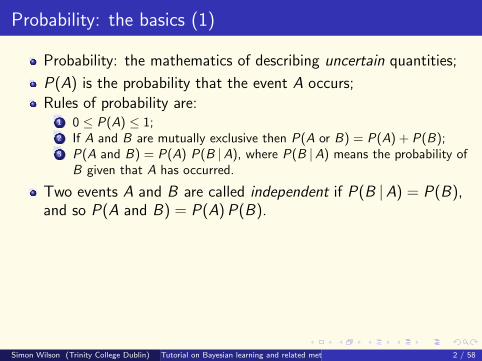
Probability: the basics (1)
Probability: the mathematics of describing uncertain quantities;
P(A) is the probability that the event A occurs;Rules of probability are:
1 0 ≤ P(A) ≤ 1;2 If A and B are mutually exclusive then P(A or B) = P(A) + P(B);3 P(A and B) = P(A) P(B |A), where P(B |A) means the probability of
B given that A has occurred.
Two events A and B are called independent if P(B |A) = P(B),and so P(A and B) = P(A) P(B).
Simon Wilson (Trinity College Dublin) Tutorial on Bayesian learning and related methods A pre-seminar for Simon Godsill’s talk2 / 58
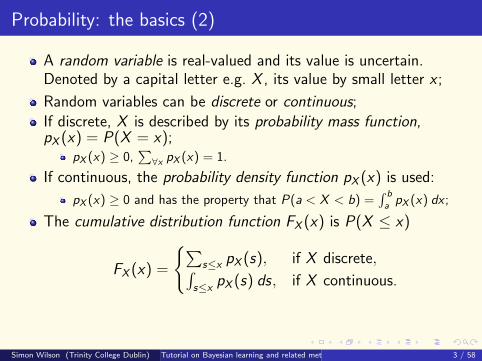
Probability: the basics (2)
A random variable is real-valued and its value is uncertain.Denoted by a capital letter e.g. X , its value by small letter x ;
Random variables can be discrete or continuous;If discrete, X is described by its probability mass function,pX (x) = P(X = x);
pX (x) ≥ 0,∑∀x pX (x) = 1.
If continuous, the probability density function pX (x) is used:
pX (x) ≥ 0 and has the property that P(a < X < b) =∫ b
apX (x) dx ;
The cumulative distribution function FX (x) is P(X ≤ x)
FX (x) =
{∑s≤x pX (s), if X discrete,∫
s≤xpX (s) ds, if X continuous.
Simon Wilson (Trinity College Dublin) Tutorial on Bayesian learning and related methods A pre-seminar for Simon Godsill’s talk3 / 58

Probability: the basics (3)
The expected value or mean of a random variable is:
E(X ) =
{∑∀x xpX (x), if X is discrete;∫∀x xpX (x) dx , if X is continuous.
It’s the ’average’ value of X , the ’centre of gravity’ of thedistribution;
The variance of X is E((X − E(X ))2):
Var(X ) =
{∑∀x(x − E(X ))2pX (x), if X is discrete;∫∀x(x − E(X ))2pX (x) dx , if X is continuous.
It’s a measure of how variable the value of X can be;
The standard deviation is√
Var(X );It has the same units of measurement as X and E(X ).
Simon Wilson (Trinity College Dublin) Tutorial on Bayesian learning and related methods A pre-seminar for Simon Godsill’s talk4 / 58

Probability: the basics (4)
Examples of discrete random variable distributions are theBernoulli, binomial and Poisson:
pX (x | p) = px(1− p)1−x , x ∈ {0, 1};
pX (x | n, p) =
(n
x
)px(1− p)n−x , x ∈ {0, 1, . . . , n};
pX (x |λ) =λx
x!e−λ, x = 0, 1, 2, . . .
Are these familiar?
Good models for many physical phenomena;
Note that they are all defined in terms of parameters — p, n, λ— we think of these as conditional distributions of X given theparameter.
Simon Wilson (Trinity College Dublin) Tutorial on Bayesian learning and related methods A pre-seminar for Simon Godsill’s talk5 / 58

Probability: the basics (5)
Examples of continuous random variable distributions are theexponential and normal (or Gaussian):
pX (x |µ) =1
µe−x/µ x ≥ 0;
pX (x |µ, σ2) =1√
2πσ2exp
(− 1
2σ2(x − µ)2
), x ∈ R.
Are these familiar?The normal distribution occurs in many places (and will in theseminar, repeatedly)
µ is its mean and σ2 is its variance;
Simon Wilson (Trinity College Dublin) Tutorial on Bayesian learning and related methods A pre-seminar for Simon Godsill’s talk6 / 58

Some normal pdf plots
Simon Wilson (Trinity College Dublin) Tutorial on Bayesian learning and related methods A pre-seminar for Simon Godsill’s talk7 / 58

Probability: the basics (6)
If we have two random variables X and Y then we can define thejoint pmf/pdf p(x , y):
For discrete X , Y , p(x , y) = P(X = x and Y = y);For continuous X , Y ,∫ b
a
∫ d
cp(x , y) dx dy = P(c < X < d , a < Y < b);
The laws of probability show that pX (x) =∫∀y p(x , y) dy ;
For discrete X and Y , the conditional distribution of X givenY = y is
P(X = x |Y = y) =p(x , y)
pY (y).
X and Y are called independent ifP(X = x |Y = y) = P(X = x) andP(Y = y |X = x) = P(Y = y);
In this case, p(x , y) = pX (x) pY (y)
Simon Wilson (Trinity College Dublin) Tutorial on Bayesian learning and related methods A pre-seminar for Simon Godsill’s talk8 / 58

Probability: two important laws (1)
Two urns: urn I has 3 red and 3 blue balls, urn II has 2 red and 4green balls;
I flip a fair coin (so P(H) = P(T ) = 1/2). If H then pick a ballfrom urn I else pick one from urn II.
What is P(R) = P(red ball picked)? By laws of probability:
P(R) = P((H and R) or (T and R))
= P(H and R) + P(T and R)
= P(H) P(R |H) + P(T ) P(R |T )
=∑
y=H,T
P(y) P(R | y)
( = 1/2× 3/6 + 1/2× 2/6 = 5/12).
Simon Wilson (Trinity College Dublin) Tutorial on Bayesian learning and related methods A pre-seminar for Simon Godsill’s talk9 / 58

Probability: two important laws (2)
Two urns: urn I has 3 red and 3 blue balls, urn II has 2 red and 4green balls;
I flip a fair coin . If H then pick a ball from urn I else pick onefrom urn II.
Now I tell you that I picked a red ball. What is the chance that Iflipped a H? This is P(H |R):
P(H |R) = P(H and R)/P(R)
=P(H) P(R |H)
P(R)
= (1/2× 3/6)/(5/12) = 3/5.
Note that if I do not tell you the ball colour, the chance of a H isP(H) = 1/2.
Observing R has allowed you to learn about how likely is H .
Simon Wilson (Trinity College Dublin) Tutorial on Bayesian learning and related methods A pre-seminar for Simon Godsill’s talk10 / 58

Probability: two important laws (3)
The first equation is an example of the partition law.
In terms of random variables, we write that for any two randomvariables X and Y :
pX (x) =∑∀y
pX |Y (x |Y = y) pY (y),
where pX |Y (x |Y = y) is the conditional pmf of X given Y .
Simon Wilson (Trinity College Dublin) Tutorial on Bayesian learning and related methods A pre-seminar for Simon Godsill’s talk11 / 58

Probability: two important laws (4)
The second equation is an example of Bayes’ law.
It can be written as:
pY |X (y |X = x) =pY (y) pX |Y (x |Y = y)
pX (x),
which is often written (by Partition law):
pY |X (y |X = x) =pY (y) pX |Y (x |Y = y)∑∀y pY (y) pX |Y (x |Y = y)
.
We also see Bayes law written as:
pY |X (y |X = x) ∝ pY (y) pX |Y (x |Y = y).∑replaced by
∫if Y is continuous.
Simon Wilson (Trinity College Dublin) Tutorial on Bayesian learning and related methods A pre-seminar for Simon Godsill’s talk12 / 58

What is Monte Carlo simulation?
This is to generate a sequence of values from a probabilitydistribution;
Usually done by computer;To Monte Carlo simulate from a probability distribution pX (x)means to generate a sequence of values x1, x2, . . . , xN such that:
The values are independentIf X discrete, the proportion of values equal to x converges to pX (x),∀x as N →∞;If X is continuous, the proportion of values in the interval (a, b)
converges to∫ b
apX (x) dx , ∀a, b as N →∞;
E.g. simulation of a die: 4, 2, 5, 5, 1, 6, 3, 4, 2 , 1, . . .
What about 1, 2, 3, 4, 5, 6, 1, 2, 3, 4, 5, 6, 1, 2, . . .?
Simon Wilson (Trinity College Dublin) Tutorial on Bayesian learning and related methods A pre-seminar for Simon Godsill’s talk13 / 58
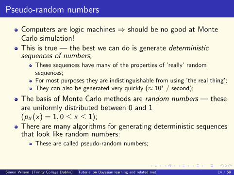
Pseudo-random numbers
Computers are logic machines ⇒ should be no good at MonteCarlo simulation!This is true — the best we can do is generate deterministicsequences of numbers;
These sequences have many of the properties of ’really’ randomsequences;For most purposes they are indistinguishable from using ’the real thing’;They can also be generated very quickly (≈ 107 / second);
The basis of Monte Carlo methods are random numbers — theseare uniformly distributed between 0 and 1(pX (x) = 1, 0 ≤ x ≤ 1);There are many algorithms for generating deterministic sequencesthat look like random numbers:
These are called pseudo-random numbers;
Simon Wilson (Trinity College Dublin) Tutorial on Bayesian learning and related methods A pre-seminar for Simon Godsill’s talk14 / 58
Methods of generating other distributions
There are many methods of generating values from otherprobability distributions: discrete, normal, exponential, etc;
All of these rely on a supply of pseudo-random numbers;
Many computer packages are able to Monte Carlo simulate frommany distributions: MATLAB, R, even Excel!
Simon Wilson (Trinity College Dublin) Tutorial on Bayesian learning and related methods A pre-seminar for Simon Godsill’s talk15 / 58

Example: discrete probability distributions
Let X be tomorrow’s weather, X ∈ {sunny, cloudy, rainy};Suppose P(X = S) = 0.2,P(X = C ) = 0.3,P(X = R) = 0.5;We can Monte Carlo simulate this distribution as follows:
Generate a (pseudo-) random number u;If u < 0.2 then X = S ;if 0.2 ≤ u < 0.5 then X = C ;if u ≥ 0.5 then X = R.
This idea is called the inverse distribution method and works forall discrete distributions.
Simon Wilson (Trinity College Dublin) Tutorial on Bayesian learning and related methods A pre-seminar for Simon Godsill’s talk16 / 58
Bayes law is the basis for learning
In the urn problem, observing R tells you something about thecoin flip but does not tell you if it’s H or T with certainty;
The question is then: how “certain” can I be that the flip is a H?Or T?
Bayes’ law allowed us to compute how certain, as a probability, interms of probabilities that we know.
This situation occurs everywhere in data analysis and is the basisof statistical inference (or statistical learning);
Bayesian statistical inference defines what we learn through aprobability distribution on the quantity of interest;
Often this is defined through Bayes’ law
Simon Wilson (Trinity College Dublin) Tutorial on Bayesian learning and related methods A pre-seminar for Simon Godsill’s talk17 / 58

Slightly more complicated example (1)
What is the temperature in this room?
For simplicity, let’s assume that it’s constant all over the room.I have a thermometer and it measures 18.1◦C ;
Is that the “real” temperature in the room?Why not?
I have another identical make of thermometer. It measures18.1◦C as well.
Should I be more certain about the value of the real temperature now?If yes then by how much?What if the second thermometer had read 18.4◦C?
Simon Wilson (Trinity College Dublin) Tutorial on Bayesian learning and related methods A pre-seminar for Simon Godsill’s talk18 / 58
Slightly more complicated example (2)
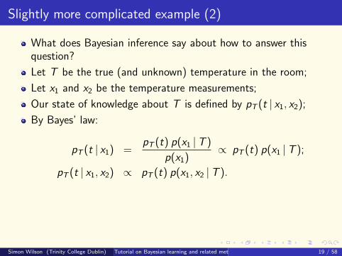
What does Bayesian inference say about how to answer thisquestion?
Let T be the true (and unknown) temperature in the room;
Let x1 and x2 be the temperature measurements;
Our state of knowledge about T is defined by pT (t | x1, x2);
By Bayes’ law:
pT (t | x1) =pT (t) p(x1 |T )
p(x1)∝ pT (t) p(x1 |T );
pT (t | x1, x2) ∝ pT (t) p(x1, x2 |T ).
Simon Wilson (Trinity College Dublin) Tutorial on Bayesian learning and related methods A pre-seminar for Simon Godsill’s talk19 / 58

Slightly more complicated example (3)
pT (t) represents what we think T is before we measure it;
This is known as the prior distribution;
For example, we are pretty sure that 0 ≤ T ≤ 40; one possibilityis a uniform distribution on this range:
pT (t) =1
40, 0 ≤ t ≤ 40.
Another is a normal distribution with mean as our best guess(say 20◦C ) and a standard deviation of 10 (so that 0 ≤ T ≤ 40with high probability)
Simon Wilson (Trinity College Dublin) Tutorial on Bayesian learning and related methods A pre-seminar for Simon Godsill’s talk20 / 58

Two possible priors for T
Simon Wilson (Trinity College Dublin) Tutorial on Bayesian learning and related methods A pre-seminar for Simon Godsill’s talk21 / 58

Slightly more complicated example (4)
p(x1, x2 |T = t) describes what we measure given the truetemperature is t;
One reasonable model is that what we measure is normallydistributed with mean T and a variance σ2;
Here we assume that we know σ2 (it says how accurate ourthermometer is — let’s say σ2 = 0.32);
p(x1 |T = t) =1√
2πσ2e−0.5(x1−t)2/σ2
.
Also assume that the two measurements are independent givenT , so that:
p(x1, x2 |T = t) = p(x1 |T = t) p(x2 | t = t)
=1
2πσ2e−
12σ2 [(x1−t)2+(x2−t)2].
Simon Wilson (Trinity College Dublin) Tutorial on Bayesian learning and related methods A pre-seminar for Simon Godsill’s talk22 / 58

Distribution of x1 when T = 18
Simon Wilson (Trinity College Dublin) Tutorial on Bayesian learning and related methods A pre-seminar for Simon Godsill’s talk23 / 58

Slightly more complicated example (5)
In Bayes’ law, the variable is t, so we should actually think ofp(x1 |T = t) and p(x1, x2 |T = t) as a function of t;
This is called the likelihood; with σ2 = 0.32 we have:
p(x1 |T = t) =1√
0.18πe−(x1−t)2/0.18.
Also assume that the two measurements are independent givenT , so that:
p(x1, x2 |T = t) = p(x1 |T = t) p(x2 | t = t)
=1
0.18πe−
10.18
[(x1−t)2+(x2−t)2].
Simon Wilson (Trinity College Dublin) Tutorial on Bayesian learning and related methods A pre-seminar for Simon Godsill’s talk24 / 58

Likelihood for x1 = 18.1
Simon Wilson (Trinity College Dublin) Tutorial on Bayesian learning and related methods A pre-seminar for Simon Godsill’s talk25 / 58

Likelihood for x1 = 18.1, x2 = 18.1
Simon Wilson (Trinity College Dublin) Tutorial on Bayesian learning and related methods A pre-seminar for Simon Godsill’s talk26 / 58

Likelihood for x1 = 18.1, x2 = 18.4
Simon Wilson (Trinity College Dublin) Tutorial on Bayesian learning and related methods A pre-seminar for Simon Godsill’s talk27 / 58

Slightly more complicated example (6)
Bayes’ law gave us:
pT (t | x1, x2) ∝ pT (t)× p(x1, x2 |T = t);
pT (t | x1, x2) is called the posterior distribution
Plots of pT (t)× p(x1, x2 |T = t) next.
Simon Wilson (Trinity College Dublin) Tutorial on Bayesian learning and related methods A pre-seminar for Simon Godsill’s talk28 / 58

pT (t)× p(x1 = 18.1 |T = t) andpT (t)× p(x1 = x2 = 18.1 |T = t)
Simon Wilson (Trinity College Dublin) Tutorial on Bayesian learning and related methods A pre-seminar for Simon Godsill’s talk29 / 58

pT (t)× p(x1 = x2 = 18.1 |T = t) andpT (t)× p(x1 = 18.1, x2 = 18.4 |T = t)
Simon Wilson (Trinity College Dublin) Tutorial on Bayesian learning and related methods A pre-seminar for Simon Godsill’s talk30 / 58
Slightly more complicated example (7)
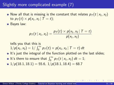
Now all that is missing is the constant that relates pT (t | x1, x2)to pT (t)× p(x1, x2 |T = t);
Bayes law:
pT (t | x1, x2) =pT (t)× p(x1, x2 |T = t)
p(x1, x2)
tells you that this is1/p(x1, x2) = 1/
∫∞0
pT (t)× p(x1, x2 |T = t) dt
It’s just the integral of the function plotted on the last slides;
It’s there to ensure that∫∞
0pT (t | x1, x2) dt = 1;
1/p(18.1, 18.1) = 55.6, 1/p(18.1, 18.4) = 68.7
Simon Wilson (Trinity College Dublin) Tutorial on Bayesian learning and related methods A pre-seminar for Simon Godsill’s talk31 / 58

p(t | x1 = x2 = 18.1) and p(t | x1 = 18.1, x2 = 18.4)
Simon Wilson (Trinity College Dublin) Tutorial on Bayesian learning and related methods A pre-seminar for Simon Godsill’s talk32 / 58

Stochastic processes
Many of the processes that we want to model occur over spaceand time:
Audio signals;Rainfall;Financial time seriesImage and video data...
These are modelled probabilistically by stochastic processes
Simon Wilson (Trinity College Dublin) Tutorial on Bayesian learning and related methods A pre-seminar for Simon Godsill’s talk33 / 58

Stochastic processes in discrete time
A very common subset is processes that evolve at discrete pointsin time t = 1, 2, 3, . . . ,T ;
Then X1,X2, . . . ,XT are the values of the process at these times;In general, we then have to define a probability distribution on(X1, . . . ,XT );
This is in general difficult because we have to define a T -dimensionalfunction p(x1, . . . , xT )
We can exploit properties of the process to make the modelsimpler to define:
Many processes obey what is called the Markov property;This means that the distribution of Xt only depends on the value ofXt−1;If X1,X2, . . . obeys this property then it’s called a Markov chain.
Simon Wilson (Trinity College Dublin) Tutorial on Bayesian learning and related methods A pre-seminar for Simon Godsill’s talk34 / 58

Markov chains
For a Markov chain:
p(x1, . . . , xT ) = p(x1) p(x2 | x1) p(x3 | x2) · · · p(xT | xT−1).
So p(x1, . . . , xT ) is defined in terms of simple one-dimensionaldistributions;If p(xt | xt−1) independent of t then we just need to define p(x1)and p(xt | xt−1);If xt is discrete-valued (say xt ∈ {1, 2, . . . , S}) then p(xt | xt−1)defined in a matrix:
P =
p11 p12 · · · p1S
p21 p22 · · · p2S...
.... . .
...pS1 pS2 · · · pSS
,
where pij = P(Xt = j |Xt−1 = i). Hence each row in P sums to1.
Simon Wilson (Trinity College Dublin) Tutorial on Bayesian learning and related methods A pre-seminar for Simon Godsill’s talk35 / 58

Example
The weather each day is: sunny (S), cloudy (C) or rainy (R);
Xt is the weather on day t;
Suppose the weather on day t depends on the weather on dayt − 1, but is independent of earlier days;
It is then a Markov chain and suppose
S C R
P =
0.3 0.5 0.20.25 0.5 0.250.4 0.3 0.3
SCR
xt−1
e.g. P(xt = S | xt−1 = R) = p31 = 0.4;
Simon Wilson (Trinity College Dublin) Tutorial on Bayesian learning and related methods A pre-seminar for Simon Godsill’s talk36 / 58

Monte Carlo simulation of our Markov chain
This is easy to do;
Define x1 (let’s make it x1 = R);
Simulate x2 given x1 (using the R row of P) — suppose wegenerate x2 = C ;
Simulate x3 given x2 (using the C row of P);
and so on.
Simon Wilson (Trinity College Dublin) Tutorial on Bayesian learning and related methods A pre-seminar for Simon Godsill’s talk37 / 58

40 days of weather
Simon Wilson (Trinity College Dublin) Tutorial on Bayesian learning and related methods A pre-seminar for Simon Godsill’s talk38 / 58
A random walk
Markov chains can have Xt continuous;
Example: Xt is normally distributed with mean Xt−1 and avariance σ2;
This is known as a random walk;
On next page is a simulation with X1 = 0 and two values of σ2
Simon Wilson (Trinity College Dublin) Tutorial on Bayesian learning and related methods A pre-seminar for Simon Godsill’s talk39 / 58

A normal random walk
Simon Wilson (Trinity College Dublin) Tutorial on Bayesian learning and related methods A pre-seminar for Simon Godsill’s talk40 / 58
Autoregressive processes
Random walks have the property that they ’wander away’ from 0(they are non-stationary);
Many physical processes tend to stay around a mean value (theyare stationary);
An autoregressive process is a simple case: Xt is normallydistributed with mean θXt−1 and a variance σ2, where−1 < θ < 1;
Higher order autoregressive processes are also very common e.g.Xt has mean θ1Xt−1 + θ2Xt−2, etc.;
These are a simple model for an audio signal.
Simon Wilson (Trinity College Dublin) Tutorial on Bayesian learning and related methods A pre-seminar for Simon Godsill’s talk41 / 58

First order autoregressive processes (with σ = 1)
Simon Wilson (Trinity College Dublin) Tutorial on Bayesian learning and related methods A pre-seminar for Simon Godsill’s talk42 / 58

Third order autoregressive processE(Xt) = 0.7Xt−1 + 0.1Xt−2 + 0.15Xt−2
Simon Wilson (Trinity College Dublin) Tutorial on Bayesian learning and related methods A pre-seminar for Simon Godsill’s talk43 / 58

Properties of Markov chains
Vast literature in probability theory on properties of Markovchains;
Here, we concentrate on one property;
Suppose I start our weather chain in day 1;
What is the weather on day t + 1? This is P(xt+1 | x1);
It turns out that the matrix of these probabilities is
P t = P × P × · · · × P (matrix multiplication).
Simon Wilson (Trinity College Dublin) Tutorial on Bayesian learning and related methods A pre-seminar for Simon Godsill’s talk44 / 58

Properties of Markov chains
Here is P t for t = 2, 20, 200: 0.30 0.46 0.240.30 0.45 0.250.32 0.44 0.24
,
0.30 0.45 0.250.30 0.45 0.250.30 0.45 0.25
,
0.30 0.45 0.250.30 0.45 0.250.30 0.45 0.25
.
Simon Wilson (Trinity College Dublin) Tutorial on Bayesian learning and related methods A pre-seminar for Simon Godsill’s talk45 / 58

Stationary distributions
So as you look further into the future:The probability that you are in each state converges to a value;This probability is the same regardless of your current state (so thechain ‘forgets’ where it was at the start);This is called the stationary distribution of the chain (in this case(0.30, 0.45, 0.25));Not all Markov chains have such a distribution;Lots of theory on conditions for which it does happen — includes mostchains that one uses in practice;
Simon Wilson (Trinity College Dublin) Tutorial on Bayesian learning and related methods A pre-seminar for Simon Godsill’s talk46 / 58

Simulating the weather Markov chain — proportion ofsunny days
Simon Wilson (Trinity College Dublin) Tutorial on Bayesian learning and related methods A pre-seminar for Simon Godsill’s talk47 / 58

Markov chains for Monte Carlo simulation
Note that the proportion of sunny days in the simulationconverges to the stationary probability of 0.302;So there is (very long winded!!) way to simulate from thedistribution (0.30, 0.45, 0.25):
Start this Markov chain in any of the 3 states;Monte Carlo simulate the chain for a ’long’ time;The state of the chain at the end of the long simulation will havedistribution (0.30, 0.45, 0.25);
Hold this thought for later!
Simon Wilson (Trinity College Dublin) Tutorial on Bayesian learning and related methods A pre-seminar for Simon Godsill’s talk48 / 58

Audio reconstruction
Think of an audio signal as a discrete process in time X1,X2, . . .;We have some audio data that has been corrupted:
CD or vinyl record scratches, tape degradation;Telephone call over a noisy line;
So what we observe are not the Xt but a corrupted versionY1, . . . ,YT ;
We want to recover the original ’true’ audio signal X1, . . . ,XT
from Y1, . . . ,YT ;
Simon Wilson (Trinity College Dublin) Tutorial on Bayesian learning and related methods A pre-seminar for Simon Godsill’s talk49 / 58

Hidden Markov models
A simple model for this process is as follows:Our real audio signal is a stochastic process like the AR model;What we actually observe Yt is normally distributed with mean Xt ;The normal distribution models the noise or degradation of the signal’The Yt ’s are independent of each other given the Xt ’s;
Mathematically:
Yt |Xt , σ2Y ∼ N(Xt , σ
2Y )
Xt |Xt−1, σ2X ∼ N(θXt−1, σ
2X ).
This is an example of a Hidden Markov Model (HMM):There is hidden Markov chain X1,X2, . . .;We observe Yt that are Xt plus some noise, and are independent;
Simon Wilson (Trinity College Dublin) Tutorial on Bayesian learning and related methods A pre-seminar for Simon Godsill’s talk50 / 58

Xt – an AR process
Simon Wilson (Trinity College Dublin) Tutorial on Bayesian learning and related methods A pre-seminar for Simon Godsill’s talk51 / 58

Xt and Yt
Simon Wilson (Trinity College Dublin) Tutorial on Bayesian learning and related methods A pre-seminar for Simon Godsill’s talk52 / 58

Yt alone
Simon Wilson (Trinity College Dublin) Tutorial on Bayesian learning and related methods A pre-seminar for Simon Godsill’s talk53 / 58

Bayesian inference (1)
Our data are the Yt ’s;
The likelihood is:
p(y1, . . . , yT | x1, . . . , xt , σ2Y )
=T∏
i=1
1√2πσ2
Y
exp
(− 1
2σ2Y
(yt − xt)2
).
We want to learn about the Xt and the 3 parameters (σ2Y , θ, σ
2X );
Simon Wilson (Trinity College Dublin) Tutorial on Bayesian learning and related methods A pre-seminar for Simon Godsill’s talk54 / 58

Bayesian inference (2)
The prior distribution for the Xt is (say) an AR process:
p(x1, . . . , xt | θ, σ2X )
=1√
2πσ2X
e−x21/2σ
2X
T∏i=2
1√2πσ2
X
e−(xt−θxt−1)2/2σ2X .
We have a prior for the 3 parameters p(σ2Y , θ, σ
2X );
Then Bayes’ law gives us:
p(x1, . . . , xT , σ2X , θ, σ
2Y | y1, . . . , yT )
=p(y1, . . . , yT | x1, . . . , xt , σ
2Y ) p(x1, . . . , xt | θ, σ2
X ) p(σ2Y , θ, σ
2X )
p(y1, . . . , yT )
Simon Wilson (Trinity College Dublin) Tutorial on Bayesian learning and related methods A pre-seminar for Simon Godsill’s talk55 / 58

Bayesian inference (3)
What is the denominator?
p(y1, . . . , yT )
=
∫p(y1, . . . , yT | x1, . . . , xt , σ
2Y ) p(x1, . . . , xt | θ, σ2
X )
× p(σ2Y , θ, σ
2X ),
a T + 3 dimensional integral;This is in general impossible to compute numerically — too big aproblem!What can we do?
For this problem, there are some algorithms that can compute themeans of the Xi , and approximate the posterior;These break down when we consider more realistic models for Xt andYt |Xt ;Can we Monte Carlo simulate fromp(x1, . . . , xT , σ
2X , θ, σ
2Y | y1, . . . , yT )?
Simon Wilson (Trinity College Dublin) Tutorial on Bayesian learning and related methods A pre-seminar for Simon Godsill’s talk56 / 58

Markov chain Monte Carlo simulation
MC simulation from high-dimensional distributions is also verydifficult;
However, it is possible to simulate from a Markov chain withstationary distribution that is the posterior;
So we simulate values of (x1, . . . , xT , σ2X , θ, σ
2Y ) according to a
certain Markov chain;
After we simulate values for a ’long time’, we are sampling fromthe posterior.
For many Bayesian learning problems, this is the only way thatwe know to approximate the solution;
This is known as MCMC (Markov chain Monte Carlo);
MCMC methods are a module in themselves!
Simon Wilson (Trinity College Dublin) Tutorial on Bayesian learning and related methods A pre-seminar for Simon Godsill’s talk57 / 58
Conclusion
I hope that this has given you an idea of some of the methodsused for Bayesian inference;
Remember: seminar is on Friday at 12pm in this room.
Simon Wilson (Trinity College Dublin) Tutorial on Bayesian learning and related methods A pre-seminar for Simon Godsill’s talk58 / 58