TTA-based Co-design Environment v1.14 User Manual - …tce.cs.tut.fi/user_manual/TCE.pdf ·...
147
Customized Parallel Computing group Department of Pervasive Computing Tampere University of Technology TTA-based Co-design Environment v1.17 User Manual Version: 32 Created: 2006-10-25 Last Modified: 2018-03-09 Document: P-1000 State: complete
Transcript of TTA-based Co-design Environment v1.14 User Manual - …tce.cs.tut.fi/user_manual/TCE.pdf ·...

Customized Parallel Computing groupDepartment of Pervasive ComputingTampere University of Technology
TTA-based Co-design Environment v1.17User Manual
Version: 32Created: 2006-10-25Last Modified: 2018-03-09Document: P-1000State: complete

TTA-based Co-design Environment v1.17 User Manual
Contents
1 INTRODUCTION 71.1 Document Overview . . . . . . . . . . . . . . . . . . . . . . . . . . . . . . . . . . . . 81.2 Acronyms, Abbreviations and Definitions . . . . . . . . . . . . . . . . . . . . . . . . . 81.3 Typographic Conventions Used in the Document . . . . . . . . . . . . . . . . . . . . . 8
2 PROCESSOR DESIGN FLOW 92.1 Design Flow Overview . . . . . . . . . . . . . . . . . . . . . . . . . . . . . . . . . . . 92.2 Main File Formats . . . . . . . . . . . . . . . . . . . . . . . . . . . . . . . . . . . . . . 11
2.2.1 Architecture Definition File (ADF) . . . . . . . . . . . . . . . . . . . . . . . . 112.2.2 TTA Program Exchange Format (TPEF) . . . . . . . . . . . . . . . . . . . . . . 112.2.3 Hardware Database (HDB) . . . . . . . . . . . . . . . . . . . . . . . . . . . . . 122.2.4 Implementation Definition File (IDF) . . . . . . . . . . . . . . . . . . . . . . . 122.2.5 Binary Encoding Map . . . . . . . . . . . . . . . . . . . . . . . . . . . . . . . 122.2.6 Operation Set Abstraction Layer (OSAL) Files . . . . . . . . . . . . . . . . . . 122.2.7 Simulation Trace Database . . . . . . . . . . . . . . . . . . . . . . . . . . . . . 132.2.8 Exploration Result Database . . . . . . . . . . . . . . . . . . . . . . . . . . . . 132.2.9 Summary of file types . . . . . . . . . . . . . . . . . . . . . . . . . . . . . . . 13
3 TUTORIALS AND HOW-TOS 143.1 TCE Tour . . . . . . . . . . . . . . . . . . . . . . . . . . . . . . . . . . . . . . . . . . 14
3.1.1 The Sample Application . . . . . . . . . . . . . . . . . . . . . . . . . . . . . . 143.1.2 Starting Point Processor Architecture . . . . . . . . . . . . . . . . . . . . . . . 153.1.3 Compiling and simulating . . . . . . . . . . . . . . . . . . . . . . . . . . . . . 153.1.4 Increasing performance by adding resources . . . . . . . . . . . . . . . . . . . . 173.1.5 Analyzing the Potential Custom Operations . . . . . . . . . . . . . . . . . . . . 193.1.6 Creating the Custom Operation . . . . . . . . . . . . . . . . . . . . . . . . . . 203.1.7 Use the custom operation in C code. . . . . . . . . . . . . . . . . . . . . . . . . 243.1.8 Adding HDL implementation of the FU to the hardware database (HDB). . . . . 263.1.9 Generating the VHDL and memory images . . . . . . . . . . . . . . . . . . . . 283.1.10 Further acceleration by adding custom operation to large TTA . . . . . . . . . . 303.1.11 Final Words . . . . . . . . . . . . . . . . . . . . . . . . . . . . . . . . . . . . . 31
3.2 From C to VHDL as Quickly as Possible . . . . . . . . . . . . . . . . . . . . . . . . . . 313.3 Hello TTA World! . . . . . . . . . . . . . . . . . . . . . . . . . . . . . . . . . . . . . . 323.4 Streaming I/O . . . . . . . . . . . . . . . . . . . . . . . . . . . . . . . . . . . . . . . . 32
3.4.1 Streaming I/O function units . . . . . . . . . . . . . . . . . . . . . . . . . . . . 333.5 Implementing Programs in Parallel Assembly Code . . . . . . . . . . . . . . . . . . . . 34
2/147 2018-03-09 version 32

TTA-BASED CO-DESIGN ENVIRONMENT
3.5.1 Preparations . . . . . . . . . . . . . . . . . . . . . . . . . . . . . . . . . . . . . 343.5.2 Introduction to DCT . . . . . . . . . . . . . . . . . . . . . . . . . . . . . . . . 343.5.3 Introduction to TCE assembly . . . . . . . . . . . . . . . . . . . . . . . . . . . 353.5.4 Implementing DCT on TCE assembly . . . . . . . . . . . . . . . . . . . . . . . 35
3.6 Using multiple memories from C code . . . . . . . . . . . . . . . . . . . . . . . . . . . 363.7 Running TTA on FPGA . . . . . . . . . . . . . . . . . . . . . . . . . . . . . . . . . . . 37
3.7.1 Simplest example: No data memory . . . . . . . . . . . . . . . . . . . . . . . . 383.7.2 Second example: Adding data memory . . . . . . . . . . . . . . . . . . . . . . 39
3.8 How to print from Altera FPGAs . . . . . . . . . . . . . . . . . . . . . . . . . . . . . . 423.8.1 Hello World 2.0 . . . . . . . . . . . . . . . . . . . . . . . . . . . . . . . . . . . 423.8.2 FPGA execution . . . . . . . . . . . . . . . . . . . . . . . . . . . . . . . . . . 433.8.3 Caveats in printing from FPGA . . . . . . . . . . . . . . . . . . . . . . . . . . 453.8.4 Summary . . . . . . . . . . . . . . . . . . . . . . . . . . . . . . . . . . . . . . 45
3.9 Designing Floating-point Processors with TCE . . . . . . . . . . . . . . . . . . . . . . 453.9.1 Restrictions . . . . . . . . . . . . . . . . . . . . . . . . . . . . . . . . . . . . . 463.9.2 Single-precision Function Units . . . . . . . . . . . . . . . . . . . . . . . . . . 463.9.3 Half-precision Support . . . . . . . . . . . . . . . . . . . . . . . . . . . . . . . 473.9.4 Half-precision Function Units . . . . . . . . . . . . . . . . . . . . . . . . . . . 473.9.5 Benchmark results . . . . . . . . . . . . . . . . . . . . . . . . . . . . . . . . . 483.9.6 Alternative bit widths . . . . . . . . . . . . . . . . . . . . . . . . . . . . . . . . 483.9.7 Processor Simulator and Floating Point Operations . . . . . . . . . . . . . . . . 49
3.10 Multi-TTA Designs . . . . . . . . . . . . . . . . . . . . . . . . . . . . . . . . . . . . . 493.11 OpenCL Support . . . . . . . . . . . . . . . . . . . . . . . . . . . . . . . . . . . . . . 493.12 System-on-a-Chip design with AlmaIF Integrator . . . . . . . . . . . . . . . . . . . . . 50
3.12.1 Generate the Processor . . . . . . . . . . . . . . . . . . . . . . . . . . . . . . . 503.12.2 Create a New Vivado Project . . . . . . . . . . . . . . . . . . . . . . . . . . . . 503.12.3 Create a Block Design . . . . . . . . . . . . . . . . . . . . . . . . . . . . . . . 513.12.4 Cleanup . . . . . . . . . . . . . . . . . . . . . . . . . . . . . . . . . . . . . . . 513.12.5 Synthesis and Implementation . . . . . . . . . . . . . . . . . . . . . . . . . . . 51
4 PROCESSOR DESIGN TOOLS 524.1 TTA Processor Designer (ProDe) . . . . . . . . . . . . . . . . . . . . . . . . . . . . . . 52
4.1.1 Starting ProDe . . . . . . . . . . . . . . . . . . . . . . . . . . . . . . . . . . . 524.1.2 Function Unit Operation Dialog . . . . . . . . . . . . . . . . . . . . . . . . . . 52
4.2 Operation Set Abstraction Layer (OSAL) Tools . . . . . . . . . . . . . . . . . . . . . . 534.2.1 Operation Set Editor (OSEd) . . . . . . . . . . . . . . . . . . . . . . . . . . . . 534.2.2 Operation Behavior Module Builder (buildopset) . . . . . . . . . . . . . . . . . 564.2.3 OSAL Tester (testosal) . . . . . . . . . . . . . . . . . . . . . . . . . . . . . . . 57
4.3 OSAL files . . . . . . . . . . . . . . . . . . . . . . . . . . . . . . . . . . . . . . . . . 574.3.1 Operation Properties . . . . . . . . . . . . . . . . . . . . . . . . . . . . . . . . 584.3.2 Operation Input Properties . . . . . . . . . . . . . . . . . . . . . . . . . . . . . 594.3.3 Operation Output Properties . . . . . . . . . . . . . . . . . . . . . . . . . . . . 604.3.4 Operation DAG . . . . . . . . . . . . . . . . . . . . . . . . . . . . . . . . . . . 604.3.5 Operation Behavior . . . . . . . . . . . . . . . . . . . . . . . . . . . . . . . . . 604.3.6 Behavior Description language . . . . . . . . . . . . . . . . . . . . . . . . . . . 61
4.4 OSAL search paths . . . . . . . . . . . . . . . . . . . . . . . . . . . . . . . . . . . . . 64
version 32 2018-03-09 3/147

TTA-based Co-design Environment v1.17 User Manual
4.5 Processor Generator (ProGe) . . . . . . . . . . . . . . . . . . . . . . . . . . . . . . . . 654.5.1 IC/Decoder Generators . . . . . . . . . . . . . . . . . . . . . . . . . . . . . . . 66
4.6 Platform Integrator . . . . . . . . . . . . . . . . . . . . . . . . . . . . . . . . . . . . . 664.7 Supported Platforms . . . . . . . . . . . . . . . . . . . . . . . . . . . . . . . . . . . . 67
4.7.1 Altera based devices . . . . . . . . . . . . . . . . . . . . . . . . . . . . . . . . 674.7.2 AlmaIFIntegrator . . . . . . . . . . . . . . . . . . . . . . . . . . . . . . . . . . 71
4.8 Hardware Database Editor (HDB Editor) . . . . . . . . . . . . . . . . . . . . . . . . . . 714.8.1 Usage . . . . . . . . . . . . . . . . . . . . . . . . . . . . . . . . . . . . . . . . 71
4.9 Hardware Database Tester . . . . . . . . . . . . . . . . . . . . . . . . . . . . . . . . . 734.9.1 Usage . . . . . . . . . . . . . . . . . . . . . . . . . . . . . . . . . . . . . . . . 734.9.2 Test conditions . . . . . . . . . . . . . . . . . . . . . . . . . . . . . . . . . . . 73
4.10 Processor unit tester . . . . . . . . . . . . . . . . . . . . . . . . . . . . . . . . . . . . . 744.10.1 Usage . . . . . . . . . . . . . . . . . . . . . . . . . . . . . . . . . . . . . . . . 74
4.11 Function Unit Interface . . . . . . . . . . . . . . . . . . . . . . . . . . . . . . . . . . . 744.11.1 Operation code order . . . . . . . . . . . . . . . . . . . . . . . . . . . . . . . . 754.11.2 Summary of interface ports . . . . . . . . . . . . . . . . . . . . . . . . . . . . . 764.11.3 Reserved keywords in generics . . . . . . . . . . . . . . . . . . . . . . . . . . . 76
5 CODE GENERATION TOOLS 775.1 TCE Compiler . . . . . . . . . . . . . . . . . . . . . . . . . . . . . . . . . . . . . . . . 77
5.1.1 Usage of TCE compiler . . . . . . . . . . . . . . . . . . . . . . . . . . . . . . 775.1.2 Custom operations . . . . . . . . . . . . . . . . . . . . . . . . . . . . . . . . . 795.1.3 Endianess Mode . . . . . . . . . . . . . . . . . . . . . . . . . . . . . . . . . . 795.1.4 Known issues . . . . . . . . . . . . . . . . . . . . . . . . . . . . . . . . . . . . 79
5.2 Binary Encoding Map Generator (BEMGenerator) . . . . . . . . . . . . . . . . . . . . 805.2.1 Usage . . . . . . . . . . . . . . . . . . . . . . . . . . . . . . . . . . . . . . . . 80
5.3 Parallel Assembler and Disassembler . . . . . . . . . . . . . . . . . . . . . . . . . . . . 805.3.1 Usage of Disassembler . . . . . . . . . . . . . . . . . . . . . . . . . . . . . . . 805.3.2 Usage of Assembler . . . . . . . . . . . . . . . . . . . . . . . . . . . . . . . . 815.3.3 Memory Areas . . . . . . . . . . . . . . . . . . . . . . . . . . . . . . . . . . . 815.3.4 General Line Format . . . . . . . . . . . . . . . . . . . . . . . . . . . . . . . . 825.3.5 Allowed characters . . . . . . . . . . . . . . . . . . . . . . . . . . . . . . . . . 825.3.6 Literals . . . . . . . . . . . . . . . . . . . . . . . . . . . . . . . . . . . . . . . 835.3.7 Labels . . . . . . . . . . . . . . . . . . . . . . . . . . . . . . . . . . . . . . . . 845.3.8 Data Line . . . . . . . . . . . . . . . . . . . . . . . . . . . . . . . . . . . . . . 845.3.9 Code Line . . . . . . . . . . . . . . . . . . . . . . . . . . . . . . . . . . . . . . 855.3.10 Long Immediate Chunk . . . . . . . . . . . . . . . . . . . . . . . . . . . . . . 865.3.11 Data Transport . . . . . . . . . . . . . . . . . . . . . . . . . . . . . . . . . . . 865.3.12 Register Port Specifier . . . . . . . . . . . . . . . . . . . . . . . . . . . . . . . 875.3.13 Assembler Command Directives . . . . . . . . . . . . . . . . . . . . . . . . . . 885.3.14 Assembly Format Style . . . . . . . . . . . . . . . . . . . . . . . . . . . . . . . 895.3.15 Error Conditions . . . . . . . . . . . . . . . . . . . . . . . . . . . . . . . . . . 915.3.16 Warning Conditions . . . . . . . . . . . . . . . . . . . . . . . . . . . . . . . . 925.3.17 Disambiguation Rules . . . . . . . . . . . . . . . . . . . . . . . . . . . . . . . 93
5.4 Program Image Generator (PIG) . . . . . . . . . . . . . . . . . . . . . . . . . . . . . . 945.4.1 Usage . . . . . . . . . . . . . . . . . . . . . . . . . . . . . . . . . . . . . . . . 94
4/147 2018-03-09 version 32

TTA-BASED CO-DESIGN ENVIRONMENT
5.4.2 Dictionary Compressor . . . . . . . . . . . . . . . . . . . . . . . . . . . . . . . 95
5.5 TPEF Dumper (dumptpef) . . . . . . . . . . . . . . . . . . . . . . . . . . . . . . . . . 96
5.5.1 Usage . . . . . . . . . . . . . . . . . . . . . . . . . . . . . . . . . . . . . . . . 96
6 CO-DESIGN TOOLS 986.1 Architecture Simulation and Debugging . . . . . . . . . . . . . . . . . . . . . . . . . . 98
6.1.1 Processor Simulator CLI (ttasim) . . . . . . . . . . . . . . . . . . . . . . . . . 98
6.1.2 Fast Compiled Simulation Engine . . . . . . . . . . . . . . . . . . . . . . . . . 99
6.1.3 Remote Debugger . . . . . . . . . . . . . . . . . . . . . . . . . . . . . . . . . 100
6.1.4 Simulator Control Language . . . . . . . . . . . . . . . . . . . . . . . . . . . . 101
6.1.5 Traces . . . . . . . . . . . . . . . . . . . . . . . . . . . . . . . . . . . . . . . . 106
6.1.6 Processor Simulator GUI (Proxim) . . . . . . . . . . . . . . . . . . . . . . . . . 107
6.2 System Level Simulation with SystemC . . . . . . . . . . . . . . . . . . . . . . . . . . 108
6.2.1 Instantiating TTACores . . . . . . . . . . . . . . . . . . . . . . . . . . . . . . . 108
6.2.2 Describing Detailed Operation Pipeline Simulation Models . . . . . . . . . . . . 109
6.3 Processor Cost/Performance Estimator (estimate) . . . . . . . . . . . . . . . . . . . . . 110
6.3.1 Command Line Options . . . . . . . . . . . . . . . . . . . . . . . . . . . . . . 110
6.4 Automatic Design Space Explorer (explore) . . . . . . . . . . . . . . . . . . . . . . . . 111
6.4.1 Explorer Application format . . . . . . . . . . . . . . . . . . . . . . . . . . . . 111
6.4.2 Command Line Options . . . . . . . . . . . . . . . . . . . . . . . . . . . . . . 112
6.4.3 Explorer Plugin: ConnectionSweeper . . . . . . . . . . . . . . . . . . . . . . . 112
6.4.4 Explorer Plugin: SimpleICOptimizer . . . . . . . . . . . . . . . . . . . . . . . 112
6.4.5 Explorer Plugin: RemoveUnconnectedComponents . . . . . . . . . . . . . . . . 113
6.4.6 Explorer Plugin: GrowMachine . . . . . . . . . . . . . . . . . . . . . . . . . . 114
6.4.7 Explorer Plugin: ImmediateGenerator . . . . . . . . . . . . . . . . . . . . . . . 114
6.4.8 Explorer Plugin: ImplementationSelector . . . . . . . . . . . . . . . . . . . . . 114
6.4.9 Explorer Plugin: MinimizeMachine . . . . . . . . . . . . . . . . . . . . . . . . 115
6.4.10 Explorer Plugin: ADFCombiner . . . . . . . . . . . . . . . . . . . . . . . . . . 115
6.4.11 Explorer Plugin: VLIWConnectIC . . . . . . . . . . . . . . . . . . . . . . . . . 115
7 PROCESSOR TEMPLATE 1177.1 Architecture Template . . . . . . . . . . . . . . . . . . . . . . . . . . . . . . . . . . . 117
7.1.1 Transport Triggered Architecture . . . . . . . . . . . . . . . . . . . . . . . . . 117
7.1.2 Immediates/Constants . . . . . . . . . . . . . . . . . . . . . . . . . . . . . . . 119
7.1.3 Operations, Function Units, and Operand Bindings . . . . . . . . . . . . . . . . 119
7.1.4 Datapath Connectivity Levels . . . . . . . . . . . . . . . . . . . . . . . . . . . 120
7.2 Programmer Interface . . . . . . . . . . . . . . . . . . . . . . . . . . . . . . . . . . . . 120
7.2.1 Default Data Address Space Layout . . . . . . . . . . . . . . . . . . . . . . . . 121
7.2.2 Instruction Address Space . . . . . . . . . . . . . . . . . . . . . . . . . . . . . 121
7.2.3 Alignment of Words in Memory . . . . . . . . . . . . . . . . . . . . . . . . . . 121
7.2.4 Stack Frame Layout . . . . . . . . . . . . . . . . . . . . . . . . . . . . . . . . 121
7.2.5 Word Byte Order . . . . . . . . . . . . . . . . . . . . . . . . . . . . . . . . . . 122
7.2.6 Function Calling Conventions . . . . . . . . . . . . . . . . . . . . . . . . . . . 123
7.2.7 Register Context Saving Conventions . . . . . . . . . . . . . . . . . . . . . . . 123
version 32 2018-03-09 5/147

TTA-based Co-design Environment v1.17 User Manual
8 PRODUCING EFFICIENT TTA DESIGNS WITH TCE 1248.1 Registers and Register Files . . . . . . . . . . . . . . . . . . . . . . . . . . . . . . . . . 1248.2 Interconnection Network . . . . . . . . . . . . . . . . . . . . . . . . . . . . . . . . . . 124
8.2.1 Negative short immediates . . . . . . . . . . . . . . . . . . . . . . . . . . . . . 1258.3 Operation Set . . . . . . . . . . . . . . . . . . . . . . . . . . . . . . . . . . . . . . . . 125
9 TROUBLESHOOTING 1269.1 Simulation . . . . . . . . . . . . . . . . . . . . . . . . . . . . . . . . . . . . . . . . . . 126
9.1.1 Failing to Load Operation Behavior Definitions . . . . . . . . . . . . . . . . . . 1269.2 Limitations of the Current Toolset Version . . . . . . . . . . . . . . . . . . . . . . . . . 126
9.2.1 Integer Width . . . . . . . . . . . . . . . . . . . . . . . . . . . . . . . . . . . . 1269.2.2 Instruction Addressing During Simulation . . . . . . . . . . . . . . . . . . . . . 1269.2.3 Data Memory Addressing . . . . . . . . . . . . . . . . . . . . . . . . . . . . . 1279.2.4 Ideal Memory Model in Simulation . . . . . . . . . . . . . . . . . . . . . . . . 1279.2.5 Guards . . . . . . . . . . . . . . . . . . . . . . . . . . . . . . . . . . . . . . . 1279.2.6 Operation Pipeline Description Limitations . . . . . . . . . . . . . . . . . . . . 1279.2.7 Encoding of XML Files . . . . . . . . . . . . . . . . . . . . . . . . . . . . . . 1279.2.8 Floating Point Support . . . . . . . . . . . . . . . . . . . . . . . . . . . . . . . 127
A FREQUENTLY ASKED QUESTIONS 128A.1 Memory Related . . . . . . . . . . . . . . . . . . . . . . . . . . . . . . . . . . . . . . 128
A.1.1 Load Store Unit . . . . . . . . . . . . . . . . . . . . . . . . . . . . . . . . . . . 128A.2 Processor Generator . . . . . . . . . . . . . . . . . . . . . . . . . . . . . . . . . . . . . 128A.3 tcecc . . . . . . . . . . . . . . . . . . . . . . . . . . . . . . . . . . . . . . . . . . . . . 128A.4 Hardware characteristics . . . . . . . . . . . . . . . . . . . . . . . . . . . . . . . . . . 129
A.4.1 Interrupt support . . . . . . . . . . . . . . . . . . . . . . . . . . . . . . . . . . 129A.5 Misc . . . . . . . . . . . . . . . . . . . . . . . . . . . . . . . . . . . . . . . . . . . . . 129
A.5.1 File Search Paths . . . . . . . . . . . . . . . . . . . . . . . . . . . . . . . . . . 129
B SystemC Simulation Example 130
C Copyright notices 135C.1 Xerces . . . . . . . . . . . . . . . . . . . . . . . . . . . . . . . . . . . . . . . . . . . . 135C.2 wxWidgets . . . . . . . . . . . . . . . . . . . . . . . . . . . . . . . . . . . . . . . . . 137C.3 L-GPL . . . . . . . . . . . . . . . . . . . . . . . . . . . . . . . . . . . . . . . . . . . . 138C.4 TCL . . . . . . . . . . . . . . . . . . . . . . . . . . . . . . . . . . . . . . . . . . . . . 143C.5 SQLite . . . . . . . . . . . . . . . . . . . . . . . . . . . . . . . . . . . . . . . . . . . . 144C.6 Editline . . . . . . . . . . . . . . . . . . . . . . . . . . . . . . . . . . . . . . . . . . . 144
BIBLIOGRAPHY 147
6/147 2018-03-09 version 32

TTA-BASED CO-DESIGN ENVIRONMENT
Chapter 1
INTRODUCTION
This is the user manual for TTA Co-design Environment (TCE) [TCE] The document describes all thetools in the toolset, and a set of common use cases in the form of tutorials.
Fig.1.1 shows a simplified overview of TCE. TCE supports programs written in C/C++ and OpenCL.User can easily design new customized Transport-Triggered Architecture (TTA) processors, compile theprogram, analyze the performance, and generate HDL implementations of the designed processors. Thegenerated application-specific processor HDL can be synthesized for example to an FPGA chip. Then,user can modify the application and upload new program image to continue development.
Application-specific instruction-set processor (ASIP) is a programmable processor which is tailored tocertain application (domain). Hence, it can outperform general-purpose processors in terms of perfor-mance, area, and power. On the other hand, the programmability and the powerful ASIP tools shouldprovide increased productivity in comparison to fixed function accelerator implementations, which offerthe highest performance.
With TCE, TTA ASIP configuration, SW compilation, and simulation can be carried out in the order ofminutes and hence most of the time can be reserved to application and architecture co-development. Itis fast to iterate over new TTA configurations, e.g., change the number and type of function units (FU),configure interconnection network (IC), register files (RF), or experiment with special function units(custom operations).
Figure 1.1: Overview of TTA Co-design Environment (TCE).
version 32 2018-03-09 7/147

TTA-based Co-design Environment v1.17 User Manual
Simple TTA designs with support for a couple of parallel arithmetic operations consume in the order ofapprox. 1000-5000 LUTs (look-up tables), which means that modern FPGA’s can easily include eventens of TTA cores. The operating clock frequency can be optimized to match the soft cores offered byFPGA vendors.
1.1 Document Overview
Chapter 2 provides an overview to the TCE processor design flow, and Chapter 3 contains tutorials forseveral common TCE use cases. These should be sufficient for starting to use the TCE toolset. The restof the chapters describe the use of each tool separately, and they can be referred to for information onmore advanced usage the tools.Many people have contributed to this document, most notably Pekka Jääskeläinen, Otto Esko, HeikkiKultala, Vladimir Guzma and Erno Salminen.
1.2 Acronyms, Abbreviations and Definitions
ADF (Processor/Machine) Architecture Definition File.BEM Binary Encoding Map. Describes the encoding of instructions.CLI Command Line InterfaceExpResDB Exploration Result Database.GUI Graphical User InterfaceGPR General Purpose RegisterHDB Hardware DatabaseHDL Hardware Description Language.HLL High Level (Programming) Language.IDF (Machine/Processor) Implementation Definition File.ILP Instruction Level Parallelism.LLVM Low Level Virtual MachineMAU Minimum Addressable UnitPIG Program Image GeneratorSQL Structured Query Language.TCE TTA Co-design Environment.TPEF TTA Program Exchange FormatTraceDB Execution Trace Database.TTA Transport Triggered Architecture.VHDL VHSIC Hardware Description Language.XML Extensible Markup Language.
1.3 Typographic Conventions Used in the Document
Style Purposeitalic parameter names in running text[brackets] bibliographic references‘single quoted’ keywords or literal strings in running text’file name’ file and directory names in running textbold Shorthand name of a TCE application.
courier UNIX commands
8/147 2018-03-09 version 32

TTA-BASED CO-DESIGN ENVIRONMENT
Chapter 2
PROCESSOR DESIGN FLOW
The main goal for the TTA Co-design Environment (TCE) is to provide a reliable and effective toolsetfor designing programmable application specific processors, and generate machine code for them fromapplications written in high-level languages, such as C, C++ or OpenCL.
In addition, TCE provides an extensible research platform for experimenting with new ideas for TransportTriggered Architectures (TTAs), retargetable ILP code generation, and application specific processordesign methodology, among others.
2.1 Design Flow Overview
The main phases in the TCE are illustrated in Figure 2.1 and listed in Table 2.1 The TCE design flowstarts from an application described in a high level language (currently the C language). The initial
TCE
tools
3rd party tools
requirements
user
Processoor designer tool (prode)
HLL (C, C++, OpenCL)
Retargerable compiler (tcecc/LLVM)
Retargerable simulator (proxim)
Processor generator (proge)
Feedback (cycle count, mem usage,)
Program image generator (pig, opt. compression)
Platform integrator (?)
FPGA synthesis tool (e.g Quartus)
HDL simulation tool (e.g QHDL)
HW database (hdb)
Platform info (FPGA-specific)
feedback
Report (FPGA resources, MHz)
Figure 2.1: Overview of TTA Co-design Environment (TCE).
version 32 2018-03-09 9/147

TTA-based Co-design Environment v1.17 User Manual
Table 2.1: Summary of tools. Some of the tools have grahical user interface (GUI) and others executedfrom the shell command line (CLI).
Tool Purpose Type Output file(s)ProDe Define FUs, registers, intercconects of TTA core GUI .adftcecc Compile software CLI .tpefProxim Simulate TTA cores (architectural level) GUI reportttasim Simulate TTA cores (architectural level) CLI reportOSEd Operation Set Abstraction Layer database editor GUI operation dbHDBEditor HW implementation database editor GUI HDBProGe / generateprocessor Generate HDL CLI (+GUI) VHDL or VerilogPIG / generatebits Generate program image CLI e.g. .mifPlatform integrator Interface with memories, generate IP-XACT CLI e.g. .xml, project files3rd party Synthesis Convert VHDL to netlist and program FPGA G/C e.g. .sof3rd party Simulation Simulate VHDL G/C report, .wave
software development phase is intended to be separate from the actual co-design flow of TCE. That is,the program is expected to be implemented and tested natively (on a workstation PC) before “porting” itto the TTA/TCE platform. The porting includes ensuring that TTA/TCE runs the program correctly, andoptimizing the hardware together with the software by modifying the resources and architecture of theprocessor to fit the application at hand – a process called hardware/software co-design.
Once the user has implemented the software based on requirements, he designs a TTA processor witha graphical tool, or selects an existing TTA, and compiles and simulates the SW. Both compiler aresimulator are retargetable so they need an architectre definition as input in addition to SW source codes.The instruction set simulator (Proxim or ttasim) produces statistics about cycle counts and utilization offunction unit, to assist in iteration of the SW of TTA HW until results are satiscatory.
The LLVM compiler framework [llv08] is used to compile the application to ’bitcode’, the intermedi-ate representation of LLVM. The resulting bitcode is then compiled and scheduled to a particular TTAprocessor by TCE. Traditional compiler optimizations are done in LLVM before bitcode generation, soit is possible to utilize the same bitcode file when exploring different TTA processors for running anapplication.
Once the performance requirement is met, the user maps the architectural resources i.e. function units andregister files, to their respective RTL implementations which are stored in Hardware Databases (HDB).The distinction between architectural models and component implementations makes it possible to haveseveral implementations, each e.g. targeted for different FPGA families or ASIC technologies, stored inHDBs. Ideally, changing the target platform might only require changes to the implementation mappingwithout any changes to the architecture.
After the implementation mapping, the Processor Generator (ProGe) can produce synthesizable HDL,which instantiates all FUS and creates the interconnection network and control unit, which is responsibleof fetching, decoding and issuing instructions. ProGe tool also includes a platform integrator featurewhich can interface the TTA with memory components of an FPGA board and create synthesis settings.Moreover, the platform integrator can “package” the TTA (and optionally also the SW) into an easilyre-usable format. In practice, this means generating IP-XACT documents which describe the details inXML. Synthesing and simulating the HDL are done with 3rd party tools, such as Altera’s Quartus andMentor Graphics’ Modelsim.
Finally, Program Image Generator (PIG) is utilized to convert the compiled SW format into actual bina-ries. PIG supports various different output formats ranging from plain binary format to FPGA vendorspecific embedded RAM formats.
More details about the tools and design phases are given in Chapters 4.1 - 6. The TCE tour tutorial insection 3.1 provides a hands-on introduction to the design flow.
10/147 2018-03-09 version 32

TTA-BASED CO-DESIGN ENVIRONMENT
2.2 Main File Formats
The flow consists of many separate tools and information is exchanged with files. This chapter gives anoverview of 8 file and database types manipulated by TCE applications and accessible to users of thetoolset, architecture definition .adf and SW binary .tpef being the most important ones. Many files areXML so user can easily access them, if needed.There a 3 kind of files:
1. HW definitions: adf, hdb, and idf
2. SW definitions: tpef, bem, opp, cc, opb
3. Simulation and exploration data: dsdb, set of the files above
2.2.1 Architecture Definition File (ADF)
Filename extension: .adf
Architecture Definition File (ADF) is a file format for defining target processor architectures, e.g. whichfunction units are used and how they are connected [CSJ04]. ADF can be created with ProDe manuallyor, e.g., by automated design space exploration tools. ADF is a specification of the target “processorarchitecture”, meaning that only the information needed to generate valid programs for the processor isstored, but nothing else. This file is needed by many tools, such as tcecc, ttasim, and ProGe.The XML snippet below gives an idea of ADF.
<adf version="1.7">
<bus name="B1"><width>32</width><guard><always-true/>
...<socket name="alu_comp_i1">
<reads-from><bus>B1</bus>
...<function-unit name="alu_comp">
<port name="in1t"><connects-to>alu_comp_i1</connects-to><width>32</width><triggers/>
...<operation>
<name>add</name><bind name="1">in1t</bind>...
<register-file name="RF"><type>normal</type>...
<address-space name="data"><width>8</width>...
2.2.2 TTA Program Exchange Format (TPEF)
Filename extension: .tpef
version 32 2018-03-09 11/147

TTA-based Co-design Environment v1.17 User Manual
TTA Program Exchange Format (TPEF) is a file format for storing compiled TTA programs which canbe either unscheduled, partially scheduled, or scheduled [Cil04]. TPEF supports auxiliary sections forstoring additional information related to the program, such as execution profiles, machine resource data,and target address space definitions. This file is needed, e.g. by ttasim and Pig.
2.2.3 Hardware Database (HDB)
Filename extension: .hdb
Hardware Database (HDB) is the main SQLite database used by the Processor Generator and the CostEstimator. The data stored in HDB consist of hardware description language definitions (HDL) of TTAcomponents (function units, register files, buses and sockets) and metadata that describe certain parame-ters used in implementations. In addition, HDB may include data of each implementation needed by thecost estimation algorithms.
TCE ships with an example HDB that includes implementations for several function units and registerfiles in VHDL, and cost data for the default interpolating cost estimation plugin.
2.2.4 Implementation Definition File (IDF)
Filename extension: .idf
Describes which implementations to use for each component in the architecture. Hence, this links ar-chitectural components described in ADF files to implementation alternatives stored in HDB. Using thisinformation it is possible to fetch correct hardware description language (HDL) files from the hardwareblock library for cost estimation and processor generation. This file is needed, by ProGe and PIG.
The XML snippet below gives an idea of IDF.
<adf-implementation>...<fu name="LSU"><hdb-file>asic_130nm_1.5V.hdb</hdb-file><fu-id>62</fu-id>
</fu>...
2.2.5 Binary Encoding Map
Filename extension: .bem
Provides enough information to produce an executable uncompressed bit image from TPEF program data.
2.2.6 Operation Set Abstraction Layer (OSAL) Files
Filename extension: .opp, .cc, .opb
OSAL stores the simulation behavior and static properties of operations that can be added to the functionunits in the designed processors.
Simulation behavior of function unit operations is described by implementing simulation functions whichcan be plugged in to the simulator run time.
The .opp file is an XML file for defining the static properties of operations (for example, how many inputsand outputs an operation has). The .cc is the C++ source file that defines the behavior model for a set ofoperations. The .opb is the plugin module compiled from the .cc. OSAL is quite complex and furtherdetails are presented in Section 4.3.
12/147 2018-03-09 version 32

TTA-BASED CO-DESIGN ENVIRONMENT
2.2.7 Simulation Trace Database
Filename extension: .tracedbStores data collected from simulations and used by instruction scheduler (profiling data) and cost estima-tor (utilization statistics, etc.).
2.2.8 Exploration Result Database
Filename extension: .dsdbExploration Result Database (ExpResDB) contains the configurations that have been evaluated duringexploration (manual or automatic) and a summary of their characteristics. Files that define each testedconfiguration (ADF and IDF) are stored in the database as well.
2.2.9 Summary of file types
Table 2.2 summarizes briefly the most common TCE file types.
Table 2.2: Summary of file typesPostfix Purpose Formatadf Architecture description XMLidf Implementation/microarchitecture description XMLhdb HW database SQLitetpef TTA program exchange format binbem Binary encoding map XMLopp Operation properties XMLcc Simulation behavior of an operation C++opb Compiled operation behavior bintracedb Database of simulation and cost estimation results SQLitedsdb Database of exploration results and TTA configurations SQLite
version 32 2018-03-09 13/147

TTA-based Co-design Environment v1.17 User Manual
Chapter 3
TUTORIALS AND HOW-TOS
This section presents 11 tutorials covering the basics, printing and streaming I/O, floating-point computa-tion, parallel assembly, multiple memories, FPGA considerations and programming TTAs using OpenCLC.
Let’s start with the simplest one.
3.1 TCE Tour
This tutorial goes through most of the tools in TCE using a fairly simple example application. It startsfrom C code and ends up with VHDL of the processor and a bit image of the parallel program. Thistutorial will also explain how to accelerate an algorithm by customizing the instruction set, i.e., by usingcustom operations. The total time to go through the tutorial is about 2−3 hours.
The tutorial file package is available at:
http://tce.cs.tut.fi/tutorial_files/tce_tutorials.tar.gz
Fetch and unpack it to a working directory and then enter the directory:
> wget http://tce.cs.tut.fi/tutorial_files/tce_tutorials.tar.gz> tar -xzf tce_tutorials.tar.gz> cd tce_tutorials/tce_tour> ls -la
total 84drwxr-xr-x 3 tce tce 4096 2010-05-28 11:40 .drwx------ 7 tce tce 4096 2012-05-18 13:22 ..-rw------- 1 tce tce 5913 2010-03-08 20:01 crc.c-rw------- 1 tce tce 1408 2008-11-07 11:35 crc.h-rw------- 1 tce tce 3286 2008-11-07 11:35 crcTable.dat-rw-r--r-- 1 tce tce 2345 2010-03-08 13:04 custom_operation_behavior.cc-rw-r--r-- 1 tce tce 855 2010-05-28 11:41 custom_operations.idf-rw------- 1 tce tce 1504 2010-03-08 20:01 main.c-rw-r--r-- 1 tce tce 45056 2010-03-10 16:09 tour_example.hdbdrwxr-xr-x 2 tce tce 4096 2010-05-28 11:40 tour_vhdl
3.1.1 The Sample Application
The test application counts a 32-bit CRC (Cyclic Redundant Check) check value for a block of data, inthis case 10 bytes. The C code implementation is written by Michael Barr and it is published under Public
14/147 2018-03-09 version 32

TTA-BASED CO-DESIGN ENVIRONMENT
Figure 3.1: Processor Designer (prode) when minimal ADF is opened
Domain. The implementation consists of two different version of crc, but we will be using the fast versiononly.
The program consists of two separate files: ’main.c’ contains the simple main function and ’crc.c’ con-tains the actual implementation. Open ’crc.c’ in your preferred editor and take a look at the code. Algo-rithm performs modulo-2 division, a byte at a time, reflects the input data (MSB becomes LSB) dependingon the previous remainder, and XORs the remainder with a predefined polynomial (32-bit constant). Themain difference between the crcSlow and crcFast implementations is that crcFast exploits a precalculatedlookup table. This is a quite usual method of algorithm optimization.
3.1.2 Starting Point Processor Architecture
Copy the ’minimal.adf’ file included in TCE distribution to a new ADF file:
cp $(tce-config --prefix)/share/tce/data/mach/minimal.adf start.adf
The file describes a minimalistic architecture containing just enough resources that the TCE compiler canstill compile programs for it. We use this minimal architecture as the starting point. Function units in’minimal.adf’ are selected from the hardware database (HDB, Section 2.2.3) so we are able to generate aVHDL implementation of the processor automatically later in the tutorial.
You can view the architecture using the graphical Processor Designer (ProDe, Section 4.1) tool:
prode start.adf &
Fig. 3.1 shows how Prode should look like. There is 1 bus and 5 units: global control unit (GCU), 2register files, 1 ALU, and 1 LSU.
You’ll learn how to edit the TTA with ProDe later in this tutorial.
If you want later to simulate the generated processor using GHDL (Section 3.1.9), you should decreasethe amount of memory in the processor already now. Otherwise the GHDL executing the generatedtestbench might consume tremendous amount of memory on your computer and even crash. Select Edit-> Address Spaces in ProDe. Then edit the bit widths of data and instruction address spaces and set themto 15 bits which should be plenty for our case.
3.1.3 Compiling and simulating
Now we want to know how well the starting point architecture executes our program. We must compilethe source code for this architecture with command:
tcecc -O3 -a start.adf -o crc.tpef -k result main.c crc.c
version 32 2018-03-09 15/147

TTA-based Co-design Environment v1.17 User Manual
Figure 3.2: Processor Simulator (proxim) when minimal ADF and crc.tpef are opened and simulated.
In addition to source codes, the compiler needs the TTA architecture definition ’start.adf’. It will producea parallel program called ’crc.tpef’ which can only be executed on this architecture. The switch −k tellsthe compiler to keep the result symbol (variable on line 29 of main.c) also in the generated program inorder to access the variable contents by name in the simulator later on.
Successful compilation does not print anything and we can now simulate the program. Let’s use graphicaluser interface version of the simulator called Proxim (Section 6.1.6):
proxim start.adf crc.tpef &
The simulator will load the architecture definition and the program and wait for commands. Proxim showsone line per instruction. Minimal TTA has only bus and hence there is only instruction slot (column). Thetotal number of instructions is about 1 200.
Execute the program by clicking “Run” and Proxim should look like Fig. 3.2. Write down this cyclecount in the bottom bar of the simulator, you can use Table 3.1. for future comparison.
You can check the result straight from the processor’s memory by writing this command to the commandline at the bottom of the simulator:
x /u w result
The command specifies the data width (4 bytes) and the result symbol we told the compiler to preservebefore. The correct checksum result is 0x62488e82.Processor resource utilization data can be viewed with command:
info proc stats
This will output a lot of information like the utilization of transport buses, register files and function units,for example:
utilizations------------buses:
16/147 2018-03-09 version 32

TTA-BASED CO-DESIGN ENVIRONMENT
Figure 3.3: Processor Simulator (proxim) shows the utilizations of each FU and bus.
B1 87.7559% (4415 writes)
sockets:lsu_i1 17.4319% (877 writes)lsu_o1 10.4949% (528 writes)...
operations executed in function units:LSU:...TOTAL 17.4319% (877 triggers)
ALU:...TOTAL 25.2037% (1268 triggers)...
register accesses:RF:0 855 reads, 0 guard reads, 1 writes...
Your output may vary depending on the compiler version, the optimizations used and your architecture.For more information on the simulator’s command line tools and syntax, you may use the
help
command.Proxim can also show othes various pieces of information about the program’s execution and its processorresource utilization. For example to check the utilization of the resources of our architecture, selectView>Machine Window from the top menu. The parts of the processor that are utilized the most arevisualized with darker red color.There are 3 basic ways to accelerate computation in TTAs:
1. Modify the algorithm itself. Beyond the scope of this tutorial.
2. Add more basic resources (FUs, RFs, buses) to TTA
3. Add custom operation(s) to TTA
3.1.4 Increasing performance by adding resources
As the current architecture is minimalistic we can increase the performance even further by adding re-sources to the processor.
version 32 2018-03-09 17/147

TTA-based Co-design Environment v1.17 User Manual
Transport buses. The architecture has only one transport bus, thus the compiler can’t exploit any in-struction level parallelism. Let’s start the architecture customization by adding another transport bus.After this there can be 2 moves per clock cycle. First copy the current architecture:
cp start.adf large.adf
and open the new architecture in ProDe:prode large.adf &
A new transport bus can be added simply by selecting the current bus and pressing “ctrl+c” to copythe bus and then pressing “ctrl+v” to paste it. Add 3 more buses. After you have added the buses youhave to connect it to the sockets. Easiest way to do this is to select “Tools->Fully connect IC”. Save thearchitecture, recompile the source code for the new architecture:
tcecc -O3 -a large.adf -o crc.tpef -k result crc.c main.c
This time simulate the program using the command line instruction set simulator:ttasim -a large.adf -p crc.tpef
The command will load the architecture and program and execute it. Once the simulation is finished, youshould see the ttasim command prompt:
> ttasim -a large.adf -p crc.tpef
(ttasim)
Now when you check the cycle count from the simulator:info proc cycles
You might see a significant drop in cycles. Also check the processor utilization statistics from the simu-lator with command:
info proc stats
Register files. From the previous simulator statistics you can see from “operations” table that there area lot of load and store operations being executed. As the architecture has only 5 general purpose registersthis tells us that there are a lot of register spilling to memory. Let’s try how the amount of registers affectthe cycle count. There are two options how we can add registers. We can either increase the number ofregisters in a register file or add a new register file.Let’s try the latter option because this way we increase the number of registers that can be accessedsimultaneously on one clock cycle. This can be done by selecting the RF and using copy and paste. Thenconnect it to the IC. Simulation statistics should indicate performance increase. As expected, the numberof load and store operations decreased. But notice also that the number of add operations decreased quitea lot. The reason is simple: addition is used to calculate stack memory addresses for the spilled registers.
Function units. Next subject for the bottleneck is the ALU as now all the basic operations are per-formed in a single function unit. From the simulator statistics you can see that logical operations and
Table 3.1: Cycle counts in different TTA configurations. You’ll fill this during the tutorial
Approx. relativeADF Cycle count cycle count Section(s) Commentstart.adf 1 3.1.3large.adf 1/2 3.1.4 start + 3 buseslarge.adf 1/5 -”- start + 3 buses + RFlarge.adf 1/6 -”- start + 3 buses + RF + new ALUcustom.adf 1/5 3.1.5 - 3.1.9large_custom.adf 1/50 3.1.10
18/147 2018-03-09 version 32

TTA-BASED CO-DESIGN ENVIRONMENT
addition are quite heavily utilized. Instead of duplicating the ALU let’s add more specific FUs from theHardware Database. Select “Edit->Add From HDB->Function Unit...”. Select a FU which has operationsand(1), ior(1), xor(1) and click “Add”. Then select FU with operation add(1) and click “Add”. Close thedialog, connect the function units and save the architecture. Recompile and simulate to see the effect oncycle count.
The architecture could be still modified even further to drop the cycle count but let’s settle for this nowand move on to custom operations.
3.1.5 Analyzing the Potential Custom Operations
Custom operations implement application specific functionality in TTA processors. This part of the tu-torial teaches how to accelerate the CRC computation by adding a custom operation to the starting pointprocessor design.
First of all, it is quite simple and efficient to implement CRC calculation entirely on hardware. Naturally,using the whole CRC function as a custom operation would be quite pointless and the benefits of using aprocessor based implementation would get smaller. Instead, we will concentrate on trying to acceleratesmaller parts of the algorithm, which is the most useful way for most algorithms.
The steps needed for custom opeation are:
1. Analyze the code for bottlenecks
2. Speculatively add a new module and operation to operation database with OSEd. Define the be-havior of the new operation (copy-paste from original code and add few macros). Optionally, youcan also simulate the operation behavior. Bind the new operation to a new function unit in ProDe
3. Modify your source code so that it utilizes the new operation and simulate. Go back to step 2 ifyou wish to explore other operations
4. Create VHDL for the operation and add it to HDB.
5. Finally, generate HDL implementation of the TTA with ProGe.
Finding the operation to be optimized is quite obvious in this case if you look at function crcFast(). Itconsists of a for-loop in which the function reflect() is called through the macro REFLECT_DATA. Ifyou look at the actual function (shown also in Fig. 3.4 you can see that it is quite simple to implement onhardware, but requires many instructions if done with basic operations in software. The function “reflects”the bit pattern around the middle point like a mirror. For example, the bit pattern 1101 0010 becomes0100 1011. The main complexity of the function is that the bit pattern width is not fixed. Fortunately, thewidth cannot be arbitrary. If you examine the crcFast()-function and the reflect macros you can spot thatfunction reflect() is only called with 8 and 32 bit widths (unsigned char and ’crc’ which is an unsignedlong).
A great advantage of TCE is that the operation semantics, processor architecture, and implementation areseparate abstractions. This simplifies designing custom operations since you can simulate your design bysimply defining the simulation behaviour of the operation and setting the latency of the operation to theprocessor architecture definition. This is nice as you do not need an actual hardware implementation ofthe operation at this point of the design, but can evaluate different custom operation possibilities at thearchitectural level. However, this brings up an awkward question: how to determine the latency of theoperation? Unrealistic or too pessimistic latency estimates can produce inaccurate performance resultsand bias the analysis.
One approach to the problem is to take an educated guess and simulate some test cases with differentcustom operation latencies. This way you can determine a latency range in which the custom operationwould accelerate your application to the satisfactory level. For example, custom operation with 1 cycledelay might give 3x speedup but 10 cycles gives just 3%. After this you can sketch how the operationcould be implemented in hardware, or consult someone knowledgeable in hardware design to figure outwhether the custom operation can be reasonably implemented within the latency constraint.
version 32 2018-03-09 19/147

TTA-based Co-design Environment v1.17 User Manual
Figure 3.4: Reflect function of CRC
Another approach is to try and determine the latency by examining the operation itself and consideringhow it could be implemented. This approach requires some insight in digital design.Besides latency you should also consider the size of the custom function unit. It will consume extra diearea, but the size limit is always case-specific, especially when area taken by memories is accounted.Accurate size estimation requires the actual HW implementation and synthesis.Let us consider the reflect function. If we had fixed width we could implement the reflect by hard wiring(and registering the output) because the operation only moves bits to other locations in the word. Thiscould be done easily in one clock cycle, as in right side of Fig. 3.4. But we need two different bit widthsso it is somewhat more complicated. We could design the HW in such way that it has two operations: onefor 8-bit data and another for 32-bit data. One way to implement this is to have 32-bit wide crosswiringand register the output. The 8-bit value would be reflected to the 8 MSB bits of the 32-bit wiring. Thenwe need to move the 8 MSB bits to the LSB end and set rest to zero. This moving can be implementedusing multiplexers. So concerning the latency this can all be done easily within one clock cycle as thereis not much logic needed.
3.1.6 Creating the Custom Operation
Now we have decided the operation to be accelerated and its latency.Next we will create a function unit implementing the operation and add it to our processor design. First,a description of the semantics of the new operation must be added at least to Operation Set AbstractionLayer (Sections 2.2.6 and 4.3). OSAL stores the semantic properties of the operation, which includes thesimulation behavior, operand count etc., but not the latency. OSAL definitions can be added by using theOSAL GUI, OSEd (Section 4.2.1).Synthesis or simulation at the VHDL level requires that at least one function unit implementing theoperation must be added to the Hardware Database (Section 2.2.3). In this tutorial we add the FU imple-mentation for our custom operation so the processor implementation can be generated, but omit the costdata required for the cost estimation. In general case, cost data should be added to cost database as well.
Using Operation Set Editor (OSEd) to add the operation data. OSEd is started with the commandosed &
Create a new operation module, which is a container for a set of operations. You can add a new modulein any of the predefined search paths, provided that you have sufficient file system access permissions.For example, choose directory ’/home/user/.tce/opset/custom’, where user is the name of the user accountbeing used for the tutorial. This directory is intended for the custom operations defined by the currentuser, and should always have sufficient access rights.
20/147 2018-03-09 version 32

TTA-BASED CO-DESIGN ENVIRONMENT
Figure 3.5: Operation Set Editor when adding new operation REFLECT32.
1. Click the root in the left area of the main window which opens list of paths. Right-click on a pathname ’/home/user/.tce/opset/custom’. A drop-down menu appears below the mouse pointer.
2. Select Add module menu item.
3. Type in the name of the module (for example, ‘tutorial’) and press OK. The module is now addedunder the selected path.
Adding the new operations. We will now add the operation definitions to the newly created operationmodule.
1. Select the module that you just added by right-clicking on its name, displayed in the left area of themain window. A drop down menu appears.
2. Select Add operation menu item.
3. Type ‘REFLECT8’ as the name of the operation.
4. Add one input by pressing the Add button under the operation input list. Select UIntWord as type.
5. Add one output by pressing the Add button under the operation output list. Select UIntWord astype.
6. After the inputs and the output of the operation have been added, close the dialog by pressing theOK button. A confirmation dialog will pop up. Press Yes to confirm the action. The operationdefinition is now added to the module.
7. Then repeat the steps for operation ‘REFLECT32’, as shown in Fig. 3.5
Defining the simulation behaviour of the operations The new operations REFLECT8 and REFLECT32do not yet have simulation behavior models, so we cannot simulate programs that use these operationswith the TCE processor simulator. Open again the operation property dialog by right-clicking RE-FLECT8, then choosing Modify properties. Now press the Open button at the bottom to open an empty
version 32 2018-03-09 21/147

TTA-based Co-design Environment v1.17 User Manual
behavior source file for the module. Copy-paste (or type if you have the time!) the following code in theeditor window:
#include "OSAL.hh"OPERATION(REFLECT8)TRIGGER
unsigned long data = UINT(1);unsigned char nBits = 8;
unsigned long reflection = 0x00000000;unsigned char bit;
/** Reflect the data about the center bit.*/for (bit = 0; bit < nBits; ++bit){
/** If the LSB bit is set, set the reflection of it.*/if (data & 0x01){
reflection |= (1 << ((nBits - 1) - bit));}
data = (data >> 1);}
IO(2) = static_cast<unsigned> (reflection);
return true;END_TRIGGER;END_OPERATION(REFLECT8)
OPERATION(REFLECT32)TRIGGER
unsigned long data = UINT(1);unsigned char nBits = 32;
unsigned long reflection = 0x00000000;unsigned char bit;
/** Reflect the data about the center bit.*/for (bit = 0; bit < nBits; ++bit){
/** If the LSB bit is set, set the reflection of it.*/if (data & 0x01){
reflection |= (1 << ((nBits - 1) - bit));}
22/147 2018-03-09 version 32

TTA-BASED CO-DESIGN ENVIRONMENT
data = (data >> 1);}
IO(2) = static_cast<unsigned> (reflection);
return true;END_TRIGGER;END_OPERATION(REFLECT32)
This code has the behaviours for the both operations. These behavior definitions reflect the input operandinteger (id 1, assigned to variable ’data’) and writes the result to the ”output operand“ (id 2, assignedfrom variable ’reflection’) which is the first output and signals the simulator that all results are computedsuccessfully.
Open file ’crc.c’ in your preferred editor. Compare the behaviour definition of reflect operations and theoriginal reflect-function. The function is mostly similar except for parameter passing and adding fewmacros added, such as OPERATION(), TRIGGER, IO(2) etc. Custom hardware operation behavior readsdata from the function unit’s input ports and writes to output ports. The value of nBits is determined fromthe operation code (REFLECT8 or REFLECT32).
Save the code and close the editor. REFLECT8 and REFLECT32 operations now have TCE simulatorbehaviour models.
Compiling operation behavior. REFLECT-operations have been added to the test module. Before wecan simulate the behavior of our operation, the C++-based behavior description must be compiled to aplugin module that the simulator can call.
1. Right-click on the module name (’tutorial’) displayed in the left area to bring up the drop downmenu.
2. Select Build menu item.
3. Hopefully, no errors were found during the compilation! Otherwise, re-open the behaviour sourcefile and try to locate the errors with the help of the diagnostic information displayed in the builddialog.
After the operation simulation model has been added and compiled the operation can be simulated. Butfor the sake of speed up we will skip the operation simulation here. Interested readers are referred toSection 4.2.1 You can close osed now.
Adding a Customized Function Unit to the Architecture. Now the operation definitions of the customoperations have been added to the Operation Set Abstraction Layer (OSAL) database. Next we need toadd at least one functional unit (FU) which implements these operations so that they can be used in theprocessor design. Note the separation between ”operation“ and an ”function unit“ that implements theoperation(s) which allows using the same OSAL operation definitions in multiple FUs with differentlatencies.
First, add the architecture of the FU that implements the custom operations to the starting point processorarchitecture. Let’s take a copy of the starting point processor design which we can freely modify and stillbe able to easily compare the architecture with and without the custom operation support later on:
cp start.adf custom.adf
Open the copy in ProDe:
prode custom.adf &
Then:
version 32 2018-03-09 23/147

TTA-based Co-design Environment v1.17 User Manual
Figure 3.6: Adding operation REFLECT8 to a new function unit in ProDe
1. Add a new function unit to the design, right click the canvas and select: Add>Function Unit. Namethe FU ”REFLECTER“. Add one output port (named output1) and one input port (trigger), to theFU in the Function unit dialog. When adding the input port, set the port as triggering by checkingthe Triggers checkbox. This port starts the execution of the operation when it is written to.
2. Add the operation ”REFLECT8“ we defined to the FU: Add from opset>REFLECT8>OK and setthe latency to 1. Click on the REFLECT8 operation and ensure that the operation input is bound tothe input ports and the output is bound to the output port. Check that the operand usage is in sucha way that input is read at cycle 0 and the result is written at the end of the cycle (can be read fromthe FU on the next cycle), as in Fig. 3.6. Thus, the latency of the operation is 1 clock cycles.
3. Repeat the previous step for operation ”REFLECT32“
4. Now an FU that supports the custom operations has been added to the architecture. Next, connectthe FU to the rest of the architecture. This can be most easliy done by selecting Tools->FullyConnect IC which connects all FUs to all the buses. Save the architecture description by clickingSave.
3.1.7 Use the custom operation in C code.
To get some benefits from the added custom hardware, we must use it from the C code. This is done byreplacing a C statement with a custom operation invocation.
Let us first backup the original C code.
cp crc.c crc_with_custom_op.c
Then open ’crc_with_custom_op.c’ in your preferred text editor.
1. Add #include “tceops.h” to the top of the file. This includes automatically generated macros whichallow us to use specific operations from C code without getting our hands dirty with inline assembly.
Usage of these macros is as follows:
24/147 2018-03-09 version 32

TTA-BASED CO-DESIGN ENVIRONMENT
_TCE_<opName>(input1, ... , inputN, output1, ... , outputN);
where <opName> is the name of the operation in OSAL. Number of input and output operandsdepends on the operation. Input operands are given first and they are followed by output operandsif any.
In our case we need to write operands into the reflecter and read the result from it. We named theoperations “REFLECT8” and “REFLECT32”, thus the macros we are going to use are as follows:
_TCE_REFLECT8(input1, output);_TCE_REFLECT32(input1, output);
Now we will modify the crcFast function to use the custom op. First declare 2 new variables at thebeginning of the function:
crc input;crc output;
These will help in using the reflect FU macro.
Take a look at the REFLECT_DATA and REFLECT_REMAINDER macros. The first one has gota magic number 8 and “variable” X is the data. This is used in the for-loop of crcFast().
The input data of reflect function is read from array message[] in the for-loop the. Let us modify thisso that at the beginning of the loop the input data is read to the input variable. Then we will use the_TCE_REFLECT8 macro to run the custom operations, and finally replace the REFLECT_DATAmacro with the output variable. After these modifications the body of the for-loop should look likethis:
input = message[byte];_TCE_REFLECT8(input, output);data = (unsigned char) output ^ (remainder >> (WIDTH - 8));remainder = crcTable[data] ^ (remainder << 8);
Next we will modify the return statement. Originally it uses REFLECT_REMAINDER macrowhere nBits is defined as WIDTH and data is remainder. Simply use _TCE_REFLECT32 macrobefore return statement and replace the original macro with the variable output:
_TCE_REFLECT32(remainder, output);return (output ^ FINAL_XOR_VALUE);
And now we are ready. Remember to save the file.
2. Compile the custom operation using C code to a parallel TTA program using the new architecturewhich includes a FU with the custom operation:
tcecc -O3 -a custom.adf -o crc_with_custom_op.tpef -k result \crc_with_custom_op.c main.c
3. Simulate the parallel program. This time we will use the command line simulator ttasim. We willalso enable writing of bus trace. It means that the simulator writes a text file containing the busvalues of the processor from every executed clock cycle. This bus trace data will be used to verifythe processor RTL implementation. Start the simulator with command:
ttasim
Then enable the bus trace setting:
setting bus_trace 1
Load architecture and program and run the simulation
version 32 2018-03-09 25/147

TTA-based Co-design Environment v1.17 User Manual
mach custom.adf
prog crc_with_custom_op.tpef
run
Verify that the result is the same as before (x /u w result). It should be the same as earlier(0x62488e82). Check the cycle count info proc cycles and compare it to the cycle count of theversion which does not use a custom operation. You should see a very noticeable drop comparedto the starting point architecture without the custom operations. Write this cycle count down for alater step and quit ttasim.
The simulator execution also created a file ’crc_with_custom_op.tpef.bustrace’ which contains thebus trace.
3.1.8 Adding HDL implementation of the FU to the hardware database (HDB).
Now we have seen that the custom operation accelerates our application. Next we’ll add a VHDL imple-mentation of the custom FU to Hardware Database (hdb). This way we will be able to generate a VHDLimplementation of our processor.If you want to skip this phase you can use the given ’tour_example.hdb’ instead of creating it yourself.Start HDBEditor (see Section 4.8):
hdbeditor &
TCE needs some data of the FU implementation in order to be able to automatically generate processorsthat include the FU.
1. function unit from ’custom.adf’ file (edit->add->FU architecture from ADF). You can leave thecheckboxes ”parametrized width“ and ”guard support“ unchecked, which is the default. Then de-fine implementation for the added function unit entry right click reflect -> Add implementation....
2. Open file ’tour_vhdl/reflect.vhdl’ that was provided in the tutorial package with the editor youprefer, and take a look. This is an example implementation of a TTA function unit performing thecustom ’reflect8’ and ’reflect32’ operations.
3. The HDB implementation dialog needs the following information from the VHDL:
1. Name of the entity and the naming of the FU interface ports.Name the implemention after the top level entity: “fu_reflect”.
By examining the VHDL code you can easily spot the clock port (clk), reset (rstx) and global lockport (glock). Operation code (opcode) port is t1opcode. Write these into the appropriate text boxes.You do not have to fill the Global lock req. port field because the function unit does not stall, i.e.does not request a global lock to the processor during its execution.
2. Opcodes.Check that the operation codes match the top of the vhdl file. REFLECT32 has operation code “0”and REFLECT8 has operation code “1”.
The operation codes must be always numbered according to the alphabetical order of the OSALoperation names, starting at 0. For example, in this case REFLECT32 is earlier than REFLECT8in the alphabetical order (i.e. 3 becomes before 8).
3. Parameters.Parameters can be found from the VHDL generics. On top of the file there is one parameter: busw.It tells the width of the transport bus and thus the maximum width of input and output operands.
Thus, add parameter named busw, type it as integer and set the value to 32 in the Parameter dialog.
4. Architecture ports.
26/147 2018-03-09 version 32

TTA-BASED CO-DESIGN ENVIRONMENT
Figure 3.7: Adding the implementation of custom operations to HW database
version 32 2018-03-09 27/147

TTA-based Co-design Environment v1.17 User Manual
These settings define the connection between the ports in the architectural description of the FUand the VHDL implementation. Each input data port in the FU is accompanied with a load portthat controls the updating of the FU input port registers.
Choose a port in the Architecture ports dialog and click edit. Name of the architecture port p1 ist1data (as in VHDL) and associated load port is t1load. Width formula is the parameter busw. Noguard port is needed in this case.
Name the output port (p2) to r1data and the width formula is now busw because the output portwrites to the bus. The output port does not have a load port.
5. Add VHDL source file.Add the VHDL source file into the Source code dialog. Notice that the HDL files must be addedin the compilation order (see section 4.8). But now we have only one source file so we can simplyadd it without considering the compilation order (Add -> Browse -> tour_vhdl/reflect.vhdl).
Now you are done with adding the FU implementation, see Fig. 3.7. Click OK.
3.1.9 Generating the VHDL and memory images
In this step we generate the VHDL implementation of the processor, and the bit image of the parallelprogram.
Select Function Unit Implementations You can either use the given ’custom_operations.idf’ includedin the tutorial files or select the implementations yourself. If you use the given file replace ’custom.idf’with ’custom_operations.idf’ in the following commands.Next, we must select implementations for all components in the architecture. Each architecture compo-nent can be implemented in multiple ways, so we must choose one implementation for each componentto be able to generate the implementation for the processor.This can be done in the ProDe tool:
prode custom.adf
Then we’ll select implementations for the FUs which can be done in Tools>Processor Implementation....Note that the selection window is not currently very informative about the different implementations, soa safe bet is to select an implementation with parametrizable width/size.
1. Selecting implementations for register files, immediate units and function units can be done twodifferent ways.
(a) Manual selection - user chooses the implementations from HDB files.i. Select implementation for RF: Click the RF name, ’Select Implementation’, find the
TCE’s default HDB file (PREFIX/share/tce/hdb/asic_130nm_1.5V.hdb) from your tceinstallation path and select an implementation for the RF from there.
ii. Next select implementation for the boolean RF like above. But this time select an imple-mentation which is guarded i.e. select an implementation which has word “guarded_0”in its name.
iii. Similarly, select implementations for the function units from TCE’s default HDB. Noticethat it is vital that you choose the implementation for LSU from the asic_130nm_1.5V.hdb.Then select implementation for the reflecter but this time you have to use the ’tour.hdb’created earlier to find the FU we added that supports the REFLECT custom operations.
(b) Automatic selection - ProDe chooses the implementations from HDB files.i. Select implementations for register files and function units all at once: Click Auto Se-
lect Implementations, find the TCE’s default HDB file from your TCE installation path(PREFIX/share/tce/hdb/asic_130nm_1.5V.hdb), make sure ’Register Files’ and ’Func-tion Units’ checkboxes are checked and press ’Find’. A dialog should appear saying 4implementations were found; 2 for register files and 2 for function units. Click ’Yes’.If the number of found implementations was under 4 in your case, refer to the manualimplementation selection above.
28/147 2018-03-09 version 32

TTA-BASED CO-DESIGN ENVIRONMENT
Figure 3.8: Generating TTA VHDL with ProGe
ii. Browse to Function Units page if you were not on it already. You should see, that reflecterFU is still without implementation (because it is not defined in asic_130nm_1.5V.hdb).Select Auto Select Implementations again, find ’tour.hdb’ as the HDB file, and press’Find’. 1 FU implementation should be found (the reflecter), click ’Yes’. Now all yourregister files and function units should have implementations.
2. Next select the IC/Decoder generator plugin used to generate the decoder in the control unit andinterconnection network: Browse... (installation_path)/share/tce/icdecoder_plugins/base/ Default-ICDecoderPlugin.so>OK. This should be selected by default.
3. Enable bus tracing from the Implementation-dialog’s IC / Decoder Plugin tab. Set the bustraceplugin parameter to “yes” and the bustracestartingcycle to “5”. The IC will now have a componentwhich writes the bus value from every cycle to a text file. Notice that this option cannot be used ifthe processor is synthesized.
You do not have to care about the HDB file text box because we are not going to use cost estimationdata.
4. Click “Save IDF...”
Generate the VHDL for the processor using Processor Generator (ProGe). You can start proces-sor generation from ProDe’s implementation selection dialog: Click “Generate Processor”. For BinaryEncoding Map: Select the “Generate new”, see Fig. 3.8
In the target directory click “Browse” and create a new directory ’proge-output’ and select it. Then clickOK to create the processor.
Or alternatively execute ProGe from command line:
generateprocessor -t -i custom.idf -o proge-output custom.adf
Flag −t generates a testbench, −i defines the implementation file, and −o the output directory. Nowdirectory ’proge-output’ includes the VHDL implementation of the designed processor except for theinstruction memory width package which will be created by Program Image Generator. You can takea look what the directory includes, how the RF and FU implementations are collected up under ’vhdl’subdir and the interconnection network has been generated to connect the units (the ’gcu_ic’ subdir). The’tb’ subdir contains testbench files for the processor core. Moreover, there are 4 shell scripts for compilingand simulating the VHDL codes in Modelsim and GHDL.
Generate instruction memory bit image using Program Image Generator. Finally, to get our shinynew processor some bits to chew on, we use generatebits to create instruction memory and data memoryimages:
version 32 2018-03-09 29/147

TTA-based Co-design Environment v1.17 User Manual
generatebits -d -w 4 -p crc_with_custom_op.tpef -x proge-output custom.adf
Flag −d creates data images, −w4 set data memory width 4 MAUs (Minimum Addressable Units, bytesin this case), −p defines the program, −x defines the HDL directory, and adf is given without a flag.
Now the file ’crc_with_custom_op.img’ includes the instruction memory image in “ascii 0/1” format.Each line in that file represents a single instruction. Thus, you can get the count of instructions bycounting the lines in that file:
wc -l crc_with_custom_op.img
Accordingly, the file ’crc_with_custom_op_data.img’ contains the data memory image of the processor.Program Image Generator also created file ’proge-output/vhdl/tta0_imem_mau_pkg.vhdl’ which containsthe width of the instruction memory (each designed TTA can have a different instruction width). The_imem_mau_pkg.vhdl file is appended with the top level entity name, which in this case is “tta0”.
Simulation and verification If you have GHDL or Modelsim installed you can now simulate the pro-cessor VHDL. First cd to proge-output directory:
cd proge-output
Then compile and simulate the testbench. With GHDL:
./ghdl_compile.sh
./ghdl_simulate.sh
Or with Modelsim:
./modsim_compile.sh
./modsim_simulate.sh
Compilation gives a couple of warnings from Synopsys’ std_arith package but that should do no harm.Simulation will take some time as the bus trace writing is enabled. If you did not change the memorywidths in Prode (Section 3.1.2 ), the simulation will crash and print “Killed”. There will be many warningsat 0ns due uninitialized signals but you can ignore them.
After simulation, you should see a message ./testbench:info: simulation stopped by --stop-timeThe simulation produces file “bus.dump” which looks like this:
0,000000001,000000042,00007ff83,00000018
...
As the testbench is ran for constant amount of cycles we need to get the relevant part out of the bus dumpfor verification. This can be done with command:
head -n <number of cycles> bus.dump > sim.dump
where the <number of cycles> is the number of cycles in the previous ttasim execution (same as lineocunt in crc_with_custom_op.tpef.bustrace). Then compare the trace dumps from the VHDL simulationand the architecture simulation:
diff -u sim.dump ../crc_with_custom_op.tpef.bustrace
If the command does not print anything the dumps were equal and the RTL simulation matches thettasim. Now you have succesfully added a custom operation, verified it, and gained a notable performanceincrease. Well done!
3.1.10 Further acceleration by adding custom operation to large TTA
As a final step, let us add the custom operation to the large TTA.
cp large.adf large_custom.adf
30/147 2018-03-09 version 32

TTA-BASED CO-DESIGN ENVIRONMENT
Figure 3.9: Processor Designer (prode) with large_custom.adf
prode large_custom.adf
Add the reflecter FU from the tour.hdb like done earlier. Fully connect the IC, as in Fig.3.9 and save.
tcecc -O3 -a large_custom.adf -o crc_with_custom_op.tpef -k result crc_with_custom_op.cmain.c
ttasim -a large_custom.adf -p crc_with_custom_op.tpef
info proc cycles
Voila! Now you have a lightning fast TTA.
3.1.11 Final Words
This tutorial is now finished. Now you should know how to customize the processor architecture byadding resources and custom operations, as well as generate the processor implementation and its in-struction memory bit image.
This tutorial used a “minimalistic” processor architecture as our starting point. The machine had only1 transport bus and 5 registers so it could not fully exploit the parallel capabilities of TTA. Then weincreased resources in the processor and the cycle count dropped to half. Adding 2 simple custom op-erations to the starting point architecture gives a similar speedup and in large machine the speedup incyclecount is about 50x.
3.2 From C to VHDL as Quickly as Possible
This tutorial introduces a fast way to generate a processor VHDL model from C source code using theDesign Space Explorer.
If you haven’t already downloaded the tutorial file package, you can get it from:http://tce.cs.tut.fi/tutorial_files/tce_tutorials.tar.gzUnpack it to a working directory and then cd to tce_tutorials/c2vhdl/
A script named c2vhdl should generate all the needed files from the C source code. The script is a bashscript using various TCE command line tools, and can be inspected for detailed instructions to generatethe VHDL and other files manually.
c2vhdl application1/complex_multiply.c
Now directory called “proge-output” should include the VHDL implementation of the processor. Thecurrent working directory should also contain the instruction memory bit image file and the instructionencoding (bem) file along with the processor architecture definition and implementation definition files.
Passing "-e" as the first parameter to c2vhdl script tells it to print estimation data, like area and energyrequirements for the processor it generates.
Tutorial is now finished and you can simulate the generated VHDL implementation of the processor witha VHDL simulator and synthesize it.
version 32 2018-03-09 31/147

TTA-based Co-design Environment v1.17 User Manual
3.3 Hello TTA World!
What would a tutorial be without the traditional “Hello World!” example? Interestingly enough, printingout “Hello World” in a standalone (operating system free) platform like the TTA of TCE is not totallystraightforward. That is the reason this tutorial is not the first one in this tutorial chapter.The first question is: where should I print the string? Naturally it is easy to answer that question whileworking with the simulator: to the simulator console, of course. However, when implementing the finalhardware of the TTA, the output is platform dependent. It can be a debugging interface, serial port output,etc.In order to make printing data easier from TTAs designed with TCE, we have included an operationcalled STDOUT in the “base operation set” that is installed with the TCE. The simulation behavior of theoperation reads its input, expects it to be a 8bit char and writes the char verbatim to the simulator host’sstandard output. Of course, in case the designer wants to use the operation in his final system he mustprovide the platform specific implementation for the function unit (FU) implementing the operation, orjust remove the FU after the design is fully debugged and verified.The default implementation of printf() in TCE uses the STDOUT operation to print out data. Therefore,implementing a “Hello World” application with TCE is as simple as adding an FU that implements theSTDOUT to the processor design and then calling printf() in the simulated program. The simulator shouldprint out the greeting as expected.Here is a simple C code (hello.c) that prints the magic string:
#include <stdio.h>
int main() {printf("Hello TTA World!");return 0;
}
Next, compile it to an architecture that implements the STDOUT. TCE ships with a minimal architecturethat also includes the STDOUT function unit, which you can use:
cp $(tce-config --prefix)/share/tce/data/mach/minimal_with_stdout.adf .tcecc --swfp -O0 hello.c -a minimal_with_stdout.adf -o hello.tpef
It should compile without errors. Beware: the compilation can take a while on a slower machine. This isbecause printf() is actually quite a large function and the compiler is not yet optimized for speed.Finally, simulate the program to get the greeting:
ttasim -a minimal_with_stdout.adf -p hello.tpef --no-debugmodeHello TTA World!
That’s it. Happy debugging!
3.4 Streaming I/O
Because TTA/TCE is an environment without operating system, there is also no file system available forimplementing file-based I/O. Therefore, one popular way to get input and output to/from the TTA is usingshared memory for communicating the data. For stream processing type of applications, one can also usean I/O function unit that implements the required operations for streaming.TCE ships with example operations for implementing stream type input/output. These operations can beused to read and write samples from streams in the designed TTA processor. The basic interface of theoperations allows reading and writing samples from the streams and querying the status of an input oroutput stream (buffer full/empty, etc.). The status operations are provided to allow the software running
32/147 2018-03-09 version 32

TTA-BASED CO-DESIGN ENVIRONMENT
in the TTA to do something useful while the buffer is empty or full, for example switch to another thread.Otherwise, in case one tries to read/write a sample from/to a stream whose buffer is empty/full, the TTAis locked and the cycles until the situation resolves are wasted.
The example streaming operations in the base operation set are called STREAM_IN, STREAM_OUT,STREAM_IN_STATUS, and STREAM_OUT_STATUS. These operations have a simulation behaviordefinition which simulates the stream I/O by reading/writing from/to files stored in the file system of thesimulator host. STREAM_IN and STREAM_OUT operations allow defining in/out files using TTASIM_STREAM_IN_FILEand TTASIM_STREAM_OUT_FILE environment variables respectively.
Here is an example C code that implements streaming I/O with the operations:
#include "tceops.h"
int main(){
char byte;int status;
while (1){
_TCE_STREAM_IN_STATUS(0, status);
if (status == 0)break;
_TCE_STREAM_IN(0, byte);_TCE_STREAM_OUT(byte);
}
return 0;}
This code uses the TCE operation invocation macros from tceops.h to read bytes from the input streamand write the same bytes to the output stream until there is no more data left. This situation is indicatedwith the status code 0 queried with the STREAM_IN_STATUS operation. The value means the streambuffer is empty, which means the file simulating the input buffer has reached the end of file.
You can test the code by creating a file <FU_NAME>.in with some test data, compiling the code andsimulating it. The code should create a copy of that file to the stream output file <FU_NAME>.out.These files should reside in the directory where the simulator is started. You can get the FU_NAME fromthe streaming function units in the adf file.
3.4.1 Streaming I/O function units
VHDL implementations and HDB entries for streaming I/O have been included in TCE since version 1.4.The stream.hdb -file in the TCE installation directory contains one function unit with STREAM_IN andSTREAM_IN_STATUS -operations, and another FU contains the STREAM_OUT and STREAM_OUT_STATUS -operations. These FUs can directly be instantiated in ProDe and synthesized on an FPGA alongwith the rest of the processor.
When these function units are instantiated in ProDe, they are realized with specific operation latencies.STREAM_IN and STREAM_OUT take 3 clock cycles, and STREAM_IN_STATUS and STREAM_OUT_STATUS execute in 1 clock cycle.
The Stream In -FU has three external ports. ext_data is 8 bits wide and is used to communicate the databyte from the external stream source to the TTA FU. When the TTA application program invokes theSTREAM_IN -operation, the ext_data signal is sampled by the FU and the Stream In -FU automaticallysends an acknowledge-signal back to the stream source through the ext_ack port of the FU. The external
version 32 2018-03-09 33/147

TTA-based Co-design Environment v1.17 User Manual
stream source is supposed to provide the next stream data value to ext_data upon noticing a rising edgein ext_ack. The three cycle latency of the operation allows some time for this to happen. Finally, the TTAapplication program can query the availability of stream data by invoking the STREAM_IN_STATUS-operation. This command reads the value of the ext_status port of the Stream In FU and the externalstream device is expected to keep the signal high in this port when there is still data available, and lowwhen the stream device has run out of data. The application program sees the status as a numerical value’1’ or ’0’.The Stream Out -FU works in a similar fashion. The ext_data port is now an output and provides the datato the external stream sink. The external stream sink is expected to sample the value of ext_data whenext_dv (data valid) is high. ext_dv is automatically operated by the FU when the application programinvokes the operation STREAM_OUT. STREAM_OUT has also a latency of 3 clock cycles to allow theexternal stream sink to take care of the data sample. Invoking the STREAM_OUT_STATUS operationsamples the signal in the ext_status -port, which the external stream sink is expected to keep high if thereis still space in the stream sink. When the stream sink is full, the signal in the ext_status -port must bepulled low by the stream sink.Having several distinct stream sources or sinks must at the moment be realized by manually copying theFUs along with their HDB and VHDL parts. The operations must have distinct names so that the compileris explicitly instructed to read from a specific source or write to a specific sink.
3.5 Implementing Programs in Parallel Assembly Code
This tutorial will introduce you to TTA assembly programming. It is recommended that you go throughthis tutorial because it will certainly familiarize you with TTA architecture and how TTA works.
3.5.1 Preparations
For the tutorial you need to download file package from http://tce.cs.tut.fi/tutorial_files/tce_tutorials.tar.gz and unpack it to a working directory. Then cd to parallel_assembly-directory.The first thing to do is to compile the custom operation set called cos16 shipped within the parallel_assembly-directory. The easiest way to do this is:
buildopset cos16
This should create a file named ’cos16.opb’ in the directory.
3.5.2 Introduction to DCT
Now you will be introduced to TCE assembler language and assembler usage. Your task is to write TCEassembly code for 2-Dimensional 8 times 8 point Discrete Cosine Transform (DCT_8x8). First take alook at the C code of DCT_8x8 ’dct_8x8_16_bit_with_sfus.c’. The code is written to support fixed pointdatatype with sign plus 15 fragment bits, which means coverage from −1 to 1− 215. The fixed pointmultiplier, function mul_16_fix, and fixed point adder, function add_16_fix, used in the code scale inputsautomatically to prevent overflow. Function cos16 takes x(2i+1) as input and returns the correspondingcosine value cos
(x(2i+1)π
16
). The code calculates following equations:
F(x) =C(x)
2
7
∑i=0
[f (i)cos
(x(2i+1)π
16
)](3.1)
F(y) =C(y)
2
7
∑i=0
[f (i)cos
(y(2i+1)π
16
)](3.2)
C(i) =
{2√2
, i = 01 ,else
. (3.3)
F(x,y) = F(x)F(y) (3.4)
34/147 2018-03-09 version 32

TTA-BASED CO-DESIGN ENVIRONMENT
3.5.3 Introduction to TCE assembly
First take a look at assembly example in file ’example.tceasm’ to get familiar with syntax. More help canbe found from section 5.3
Compilation of the example code is done by command:
tceasm -o example.tpef dct_8x8_16_bit_with_sfus.adf example.tceasm
The assembler will give some warnings saying that “Source is wider than destination.” but these can beignored.
The compiled tceasm code can be simulated with TCE simulator, ttasim or proxim(GUI).
ttasim -a dct_8x8_16_bit_with_sfus.adf -p example.tpef , or
proxim dct_8x8_16_bit_with_sfus.adf example.tpef
It is recommended to use proxim because it is more illustrating to track the execution with it. Especiallyif you open the Machine Window (View -> Machine Window) and step through the program.
Check the result of example code with command (you can also write this in proxim’s command line atthe bottom of the main window):
x /a IODATA /n 1 /u b 2 .
the output of x should be 0x40.
3.5.4 Implementing DCT on TCE assembly
Next try to write assembly code which does the same functionality as the C code. The assembly codemust be functional with the given machine ’dct_8x8_16_bit_with_sfus.adf’. Take a look at the processorby using prode:
prode dct_8x8_16_bit_with_sfus.adf &
The processor’s specifications are the following:
Supported operationsOperations supported by the machine are: mul, mul_16_fix, add, add_16_fix, ldq, ldw, stq, stw, shr, shl,eq, gt, gtu, jump, cos16 and immediate transport.
When you program using TTA assembly you need to take into account operation latencies. The jumplatency is four clock cycles and load latencies (ldq and ldw) are three cycles. Latency for multiplications(mul and mul_16_fix) are two clock cycles.
Address spacesThe machine has two separate address spaces, one for data and another for instructions. The data memoryis 16-bit containing 128 memory slots and the MAU of data memory is 16-bits. The instruction memoryhas 1024 memory slots which means that the maximum number of instructions of 1024.
Register filesThe machine contains 4 register files, each of which have 4 16-bit registers, leading to total of 16 16-bitregisters. The first register file has 2 read ports.
Transport busesThe machine has 3 16-bit buses, which means maximum of 3 concurrent transports. Each bus can containa 8-bit short immediate.
ImmediatesBecause the transport buses can only contain 8-bit short immediates you must use the immediate unit ifyou want to use longer immediates. The immediate unit can hold a 16-bit immediate. There is an exampleof immediate unit usage in file ’immediate_example.tceasm’. Basically you need to transfer the value tothe immediate register. The value of immediate register can be read on the next cycle.
The initial input data is written to memory locations 0-63 in the file ’assembler_tutorial.tceasm’. Writeyour assembly code in that file.
version 32 2018-03-09 35/147

TTA-based Co-design Environment v1.17 User Manual
3.5.4.1 Verifying the assembly program
The reference output is given in ’reference_output’. You need to compare your assembly program’ssimulation result to the reference output. Comparision can be done by first dumping the memory contentsin the TCE simulator with following command:
x /a IODATA /n 64 /u b 0
The command assumes that output data is stored to memory locations 0-63.
The easiest way to dump the memory into a text file is to execute ttasim with the following command:
ttasim -a dct_8x8_16_bit_with_sfus.adf -p assembler_tutorial.tpef < input_command.txt> dump.txt
After this you should use sed to divide the memory dump into separete lines to help comparison betweenyour output and the reference output. Use the following command to do this (there is an empty spacebetween the first two slashes of the sed expression):
cat dump.txt | sed ’s/ / \n/g’ > output.txt
And then compare the result with reference:
diff -u output.txt reference_output
When the TCE simulator memory dump is the same as the reference output your assembly code works andyou have completed this tutorial. Of cource you might wish to improve your assembly code to minimizecycle count or/and instruction count.
You should also compile the C program and run it because it gives more detailed information which canbe used as reference data if you need to debug your assembly code.
To compile the C code, enter:
gcc -o c_version dct_8x8_16_bit_with_sfus.c
If you want the program to print its output to a text file, you can use the following command:
./c-version > output.txt
To get some idea of the performance possibilities of the machine, one assembly code has 52 instructionsand it runs the DCT8x8 in 3298 cycles.
3.6 Using multiple memories from C code
TCE supports accessing multiple address spaces from C code via the __attribute__((address_space(N))extension. The numerical id from the attribute is used to connect the memory reference to the ADFaddress space using the XML element numerical-id. There can be one or more numerical ids mapped toa single ADF address space.
The following is from an ADF with three separate data address spaces with numerical ids 0, 1, and 2. Thenumerical id 0 is reserved for the default data address space which stores the stack, heap and the globalconstant data.
<address-space name="data"><width>8</width><min-address>0</min-address><max-address>16777215</max-address><numerical-id>0</numerical-id>
</address-space>
<address-space name="data1"><width>8</width><min-address>0</min-address><max-address>65535</max-address><numerical-id>1</numerical-id>
</address-space>
36/147 2018-03-09 version 32

TTA-BASED CO-DESIGN ENVIRONMENT
<address-space name="data2"><width>8</width><min-address>0</min-address><max-address>16383</max-address><numerical-id>2</numerical-id>
</address-space>
The address spaces can be referred to from the C program with code like this:
#include <stdio.h>
#define ASIZE 4
volatile int space0[ASIZE] __attribute__((address_space(0)));volatile int space0_1[ASIZE] __attribute__((address_space(0)));volatile int space1[ASIZE] __attribute__((address_space(1)));volatile int space1_1[ASIZE] __attribute__((address_space(1)));volatile int space2[ASIZE] __attribute__((address_space(2)));volatile int space2_1[ASIZE] __attribute__((address_space(2)));
int main() {int i = 0;
/* The start addresses of the tables should overlap asthey are allocated in different address spaces. */
iprintf("space0@%x space0_1@%x space1@%x space1_1@%x space2@%x space2_1@%x\n",(unsigned)space0, (unsigned)space0_1, (unsigned)space1, (unsigned)space1_1,(unsigned)space2, (unsigned)space2_1);
return 0;}
The effect of having multiple disjoint address spaces is visible when simulating the code as the arraysallocated to the different memories share the same addresses but different storage:
space0@a84 space0_1@a94 space1@4 space1_1@14 space2@4 space2_1@14
The space0 array is stored in the default address space. In the beginning of the default address space thereis usually some global data for some C library functions such as the iprintf or the emulation library, thusending up with the start address of 0xa84 for the array0. For the extra address spaces 1 and 2, the arraysstart from 4 which is the first valid storage address in those address spaces. Storing data to address 0 isnot done to avoid problems with NULL pointers pointing to valid data (in this case space1 and space2would have been stored at address 0 = NULL).
When using custom operation calls to manually execute operations that access memory on processors thathave multiple data address spaces, it should be done using _TCEAS_OPERATIONNAME macro insteadof using _TCE_OPERATIONNAME macro. See section 5.1.2 for more information about these customoperation call macros.
3.7 Running TTA on FPGA
This tutorial illustrates how you can run your TTA designs on a FPGA board. Tutorial consists of twosimple example sections and a more general case description section.
Download the tutorial file package from:
version 32 2018-03-09 37/147

TTA-based Co-design Environment v1.17 User Manual
http://tce.cs.tut.fi/tutorial_files/tce_tutorials.tar.gz
Unpack it to a working directory and cd to tce_tutorials/fpga_tutorial
3.7.1 Simplest example: No data memory
3.7.1.1 Introduction
This is the most FPGA board independent TTA tutorial one can make. The application is a simple ledblinker which has been implemented using register optimized handwritten TTA assembly. In other wordsthe application doesn’t need a load store unit so there is no need to provide data memory. In addition theinstruction memory will be implemented as a logic array.
3.7.1.2 Application
The application performs a 8 leds wide sweep in an endless loop. Sweep illuminates one led at a time andstarts again from first led after reaching the last led. There is also a delay between the iterations so thatthe sweep can be seen with human eye.
As stated in the introduction the application is coded in assembly. If you went through the assemblytutorial the code is probably easy to understand. The code is in file ’blink.tceasm’. The same applicationis also written in C code in file ’blink.c’.
3.7.1.3 Create TTA processor core and instruction image
The architecture we’re using for this tutorial is ’tutorial1.adf’. Open it in ProDe to take a look at it:
prode tutorial1.adf
As you can see it is a simple one bus architecture without a LSU. There are also 2 “new” functionunits: rtimer and leds. Rtimer is a simple tick counter which provides real time clock or countdowntimer operations. Leds is function unit that can write ’0’ or ’1’ to FPGA output port. If those ports areconnected to leds the FU can control them.
Leds FU requires a new operation definition and the operation is defined in ’led.opp’ and ’led.cc’. Youneed to build this operation defintion:
buildopset led
Now you can compile the assembly code:
tceasm -o asm.tpef tutorial1.adf blink.tceasm
If you wish you can simulate the program with proxim and see how it works but the program runs inendless loop and most of the time it stays in the “sleep” loop.
Now you need to select implementations for the function units. This can be done in ProDe. See TCEtour section 3.1.9 for more information. Implementations for leds and rtimer are found from the fpga.hdbshipped with the tutorial files. Notice that there are 2 implementations for the rtimer. ID 3 is for 50 MHzclock frequency and ID 4 for 100 MHz. All other FUs are found from the default hdb.
Save the implementation configuration to ’tutorial1.idf’.
Next step is to generate the VHDL implementation of the processor:
generateprocessor -i tutorial1.idf -o asm_vhdl/proge-output tutorial1.adf
Then create the proram image:
generatebits -f vhdl -p asm.tpef -x asm_vhdl/proge-output tutorial1.adf
Notice that the instruction image format is “vhdl” and we request generatebits to not create data image atall. Now, move the generated ’asm_imem_pkg.vhdl’ to the asm_vhdl directory and cd there.
mv asm_imem_pkg.vhdl asm_vhdl/
cd asm_vhdl
38/147 2018-03-09 version 32

TTA-BASED CO-DESIGN ENVIRONMENT
3.7.1.4 Final steps to FPGA
We have successfully created the processor core and instruction memory image. Now we need an instruc-tion memory component that can use the generated image. Luckily you don’t have to create it as it isshipped with the tutorial files. The component is in file ’inst_mem_logic.vhd’ in asm_vhdl directory andit can use the generated ’asm_imem_pkg.vhdl’ without any modifications.
Next step is to connect TTA toplevel core to the memory component and connect the global signals outfrom that component. This has also been done for you in file ’tutorial_processor1.vhdl’. If you are curioushow this is done open the file with your preferred text editor. All the signals coming out of this componentare later connected to FPGA pins.
Now you need to open your FPGA tool vendor’s FPGA design/synthesis program and create a new projectfor your target FPGA. Add the three files in asm_vhdl-directory (toplevel file ’tutorial_processor1.vhdl’,’inst_mem_logic.vhd’ and ’asm_imem_pkg.vhdl’) and all the files in proge-output/gcu_ic/ and proge-output/vhdl directories to the project. The toplevel entity name is ’tutorial_processor1’.
Then connect the toplevel signals to appropriate FPGA pins. The pins are most probably described inthe FPGA board’s user manual. Signal ’clk’ is obviously connected to the pin that provides clock signal.Signal ’rstx’ is the reset signal of the system and it is active low. Connect it to a switch or pushbuttonthat provides ’1’ when not pressed. Signal bus ’leds’ is 8 bits wide and every bit of the bus should beconnected to an individual led. Don’t worry if your board doesn’t have 8 user controllable leds, you canleave some of them unconnected. In that case all of the leds are off some of the time.
Compile and synthesize your design with the FPGA tools, program your FPGA and behold the lightshow!
3.7.2 Second example: Adding data memory
In this tutorial we will implement the same kind of system as above but this time we include data memoryand use C coded application. Application has the same functionality but the algorithm is a bit different.This time we read the led pattern from a look up table and to also test store operation the pattern is storedback to the look up table. Take a look at file ’blink_mem.c’ to see how the timer and led operations areused in C code.
3.7.2.1 Create TTA processor core and binary images
The architecture for this tutorial is ’tutorial2.adf’. This architecture is the same as ’tutorial1.adf’ with theexception that now it has a load store unit to interface it with data memory.
You need to compile the operation behaviour for the led function unit if you already haven’t done it:
buildopset led
Then compile the program:
tcecc -O3 -a tutorial2.adf -o blink.tpef blink_mem.c
Before you can generate processor vhdl you must select implementations for the function units. Open thearchitecture in ProDe and select Tools->Processor Implementation...
prode tutorial2.adf
It is important that you choose the implementation for LSU from the fpga.hdb shipped with the tutorialfiles. This implementation has more FPGA friendly byte enable definition. Also the implementations forleds and timer FUs are found from fpga.hdb. As mentioned in the previous tutorial, timer implementationID 3 is meant for 50 MHz clock frequency and ID 4 for 100 MHz clock. Other FUs are found from thedefault hdb.
Generate the processor VHDL:
generateprocessor -i tutorial2.idf -o c_vhdl/proge-output tutorial2.adf
Next step is to generate binary images of the program. Instruction image will be generated again asa VHDL array package. But the data memory image needs some consideration. If you’re using anAltera FPGA board the Program Image Generator can output Altera’s Memory Initialization Format
version 32 2018-03-09 39/147

TTA-based Co-design Environment v1.17 User Manual
(mif). Otherwise you need to consult the FPGA vendor’s documentation to see what kind of format isused for memory instantiation. Then select the PIG output format that you can convert to the neededformat with the least amount of work. Of course you can also implement a new image writer class toPIG. Patches are welcome.
Image generation command is basically the following:
generatebits -f vhdl -d -w 4 -o mif -p blink.tpef -x c_vhdl/proge-output tutorial2.adf
Switch ’-d’ tells PIG to generate data image. Switch ’-o’ defines the data image output format. Changeit to suit your needs if necessary. Switch ’-w’ defines the width of data memory in MAUs. By defaultMAU is assumed to be 8 bits and the default LSU implementations are made for memories with 32-bitdata width. Thus the width of data memory is 4 MAUs.
Move the created images to the vhdl directory:
mv blink_imem_pkg.vhdl c_vhdl/
mv blink_data.mif c_vhdl/
3.7.2.2 Towards FPGA
Go to the vhdl directory:
cd c_vhdl
TTA vhdl codes are in the proge-output directory. Like in the previous tutorial file ’inst_mem_logic.vhd’holds the instruction memory component which uses the created ’blink_imem_pkg.vhdl’. File ’tuto-rial_processor2.vhdl’ is the toplevel design file and again the TTA core toplevel is connected to the in-struction memory component and global signals are connected out from this design file.
Creating data memory componentVirtually all FPGA chips have some amount of internal memory which can be used in your own designs.FPGA design tools usually provide some method to easily create memory controllers for those internalmemory blocks. For example Altera’s Quartus II design toolset has a MegaWizard Plug-In Managerutility which can be used to create RAM memory which utilizes FPGA’s internal resources.
There are few points to consider when creating a data memory controller:
1. Latency. Latency of the memory should be one clock cycle. When LSU asserts a read commandthe result should be readable after one clock cycle. This means that the memory controller shouldn’tregister the memory output because the registering is done in LSU. Adding an output register wouldincrease read latency and the default LSU wouldn’t work properly.
2. Address width. As stated before the minimal addressable unit from the TTA programmer’s pointof view is 8 bits by default. However the width of data memory bus is 32 bits wide in the defaultimplementations. This also means that the address bus to data memory is 2 bits smaller because itonly needs to address 32-bit units. To convert 8-bit MAU addresses to 32-bit MAU addresses oneneeds to leave the 2 bits out from LSB side.
How this all shows in TCE is that data memory address width defined in ADF is 2 bits wider thanthe actual address bus coming out of LSU. When you are creating the memory component youshould consider this.
3. Byte enable. In case you were already wondering how can you address 8-bit or 16-bit wide areasfrom a 32-bit addressable memory the answer is byte enable (or byte mask) signals. These signalscan be used to enable individual bytes from 32-bit words which are read from or written to thememory. And those two leftover bits from the memory address are used, together with the memoryoperation code, to determine the correct byte enable signal combination.
When you are creating the memory controller you should add support for byte enable signals.
4. Initialization. Usually the internal memory of FPGA can be automatically initialized during FPGAconfiguration. You should find an option to initialize the memory with a specific initialization file.
40/147 2018-03-09 version 32

TTA-BASED CO-DESIGN ENVIRONMENT
Connecting the data memory componentNext step is to interface the newly generated data memory component to TTA core. LSU interface is thefollowing:
fu_lsu_data_in : in std_logic_vector(fu_lsu_dataw-1 downto 0);fu_lsu_data_out : out std_logic_vector(fu_lsu_dataw-1 downto 0);fu_lsu_addr : out std_logic_vector(fu_lsu_addrw-2-1 downto 0);fu_lsu_mem_en_x : out std_logic_vector(0 downto 0);fu_lsu_wr_en_x : out std_logic_vector(0 downto 0);fu_lsu_bytemask : out std_logic_vector(fu_lsu_dataw/8-1 downto 0);
Meanings of these signals are:
Signal name Descriptionfu_lsu_data_in Data from the memory to LSUfu_lsu_data_out Data from LSU to memoryfu_lsu_addr Address to memoryfu_lsu_mem_en_x Memory enable signal which is active low. LSU asserts this signal to ’0’ when
memory operations are performed. Otherwise it is ’1’. Connect this to memoryenable or clock enable signal of the memory controller.
fu_lsu_wr_en_x Write enable signal which is active low. During write operation this signalis ’0’. Read operation is performed when this signal ’1’. Depending on thememory controller you might need to invert this signal.
fu_lsu_bytemask Byte mask / byte enable signal. In this case the signal width is 4 bits and eachbit represents a single byte. When the enable bit is ’1’ the corresponding byteis enabled and value ’0’ means that the byte is ignored.
Open file ’tutorial_processor2.vhdl’ with your preferred text editor. From the comments you can seewhere you should add the memory component declaration and component instantiation. Notice that thoseLSU signals are connected to wires (signals with appendix ’_w’ in the name). Use these wires to connectthe memory component.
Final stepsAfter you have successfully created the data memory component and connected it you should add therest of the design VHDL files to the design project. All of the files in proge-output/gcu_ic/ and proge-output/vhdl/ directories need to be added.
Next phase is to connect toplevel signals to FPGA pins. Look at the final section of the previous tutorialfor more verbose instructions how to perform pin mapping.
Final step is to synthesize the design and configure the FPGA board. Then sit back and enjoy the lightshow.
3.7.2.3 More to test
If you simulate the program you will notice that the program uses only STW and LDW operations. Reasonfor this can be easily seen from the source code. Open ’blink_mem.c’ and you will notice that the lookup table ’patterns’ is defined as ’volatile unsigned int’. If you change this to ’volatile unsigned char’ or’volatile unsigned short int’ you can test STQ and LDQU or STH and LDHU operations. Using theseoperations also means that the LSU uses byte enable signals.
Whenever you change the source code you need to recompile your program and generate the binaryimages again. And move the images to right folder if it’s necessary.
In addition you can compile the code without optimizations. This way the compiler leaves function callsin place and uses stack. The compilation command is then:
tcecc -O0 -a tutorial2.adf -o blink.tpef blink_mem.c
version 32 2018-03-09 41/147

TTA-based Co-design Environment v1.17 User Manual
3.8 How to print from Altera FPGAs
TCE comes with a special function unit which enables character output from Altera FPGAs. This SFUutilizes Altera JTAG UART IP core and nios2-terminal host program for this functionality. Neither ofthem are included in TCE so you need the appropriate Altera software and libraries (namely Quartus IIand Nios II EDS) in order to use the printing capability.
3.8.1 Hello World 2.0
If you haven’t already downloaded the tutorial file package, you should download it now from:http://tce.cs.tut.fi/tutorial_files/tce_tutorials.tar.gz
Then unpack it to a working directory and cd to tce_tutorials/fpga_stdoutLet’s begin by examining our tutorial architecture. Open the given test.adf architecture in ProDe:
prode test.adf &
As you can see, the architecture includes IO function unit which implements the STDOUT operation. Inaddition the architecture also has a timer function unit which we will also be used in this tutorial.
3.8.1.1 Examine the first version
Open source code file ’std_print.c’ in your preferred text editor. As you can see, the code includes ’stdio.h’and uses printf() for printing “Hello World!”. Furthermore, operation RTC is used to measure how longthe printing takes and this time is then printed at the end of the program. Writing value “0” to the RTCresets the real time clock in timer FU. When the RTC is invoked with a non-zero value, the current time iswritten to the given variable (in this case to variable “timestamp”). RTC counts the time in millisecondsand by default, the instruction set simulator assumes clock frequency of 100 MHz.Now compile the source code with the following command:
tcecc -O0 --swfp -a test.adf -o std_print.tpef std_print.c
The compilation command contains a few flags that should be explained in more detail. Let’s first lookinto the --swfp flag: this tells the compiler to link the program with the floating point emulation library.Floating point support is needed because printf() function includes support for printing floating pointvalues and our architecture does not contain floating point function units. To emphasize the lesson ofthis tutorial it is important that you compile the code without optimizations i.e. with -O0 flag. Otherwiseour witty compiler will optimize the first printf() call (which just prints a constant character string) intoinlined _TCE_STDOUT operations.After compiling, execute the program in the instruction set simulator:
ttasim -a test.adf -p std_print.tpef
You should see the printed text in your terminal. By the time of writing this tutorial, the duration of the“Hello World” printing with printf() took 61 ms (time may vary depending on the TCE version).But speaking of the lesson, execute the following command to examine the minimum memory consump-tion of this program:
dumptpef -m std_print.tpef
As you should notice, the instruction count is high (around 45 000 at the time of writing this tutorial) onthis simple sequential TTA architecture with optimizations disabled. Major part of the instructions arespent on the printf() and floating point emulation functions.First step in reducing the instruction count is to use iprintf() instead of printf(). Function iprintf() isa simplified version of printf() which drops the support for printing floating points. In our test case wedon’t need to print floats, so open the source code file ’std_print.c’ in your preferred text editor and changethe two printf() calls to iprintf(). Alternatively, you can do this with program sed:
sed -i ’s/printf/iprintf/g’ std_print.c
42/147 2018-03-09 version 32

TTA-BASED CO-DESIGN ENVIRONMENT
Now recompile the program and check the instruction count:
tcecc -O0 -a test.adf -o std_print.tpef std_print.c
dumptpef -m std_print.tpef
You should see a significant drop in the instruction count. If you simulate the new program, you noticeno difference in the behavior (except that the measured time might be a bit lower).
3.8.1.2 Light weight printing
TCE includes a Light Weigth PRinting (lwpr) library to provide small and simple functions for printingstrings and integers for further reducing the instruction count overhead of print support. Take a look atthe source code file ’lightweight_print.c’ to see how these functions are used. The library is includedwith header ’lwpr.h’. Function lwpr_print_str() is utilized to output strings and function lwpr_print_int()is used for printing integers. There is also function for printing integers in hexadecimal format calledlwpr_print_hex(), but it is not used in this tutorial.
Compile the new code to see the difference of using lwpr:
tcecc -O0 -llwpr -a test.adf -o lightweight_print.tpef lightweight_print.c
Notice the new compilation flag -llwpr for including the light weight printing library.
First, check the instruction count with:
dumptpef -m lightweight_print.tpef
You should notice that the instruction count has dropped dramatically and also the initialized data memoryis a lot smaller that previously.
Next, simulate program:
ttasim -a test.adf -p lightweight_print.tpef
Printed text is the same as previously except that the measured duration has dropped significantly.
3.8.2 FPGA execution
Next step is to get the program running on an FPGA. Prerequisite for this step is that you have AlteraQuartus II and nios2-terminal programs installed and you have a Stratix II DSP FPGA board. But don’tworry if you don’t have this specific board, this tutorial can be completed with other Altera FPGA boardsas well. In case you are using alternative board you must do a few manual changes before synthesizingand executing the design. Disclaimer: we assume no liability in case you fry your FPGA :)
3.8.2.1 Preparations
Before starting to generate the processor we first must adjust the address space sizes of the architecture.In order to do this, open the architecture in ProDe and open the address space dialog (Edit -> AddressSpaces...).
prode test.adf &
Adjust both the data and instruction address space to be 10 bits wide. This should be enough for ourapplication according to the dumptpef output.
Next recompile the application so it adapts to the new address space sizes:
tcecc -O0 -llwpr -a test.adf -o lightweight_print.tpef lightweight_print.c
If you wish you can execute the program with ttasim to verify that it still works after the address spacesizes changed.
Before generating the processor, you must also select the RF and FU implementations. If you wish toskip this step, you can use the given IDF by renaming it:
mv preselected.idf test.idf
Then move on to section 3.8.2.2. If you choose to learn and do this step manually, keep following theinstructions. In case you don’t already have the architecture open, do it now:
version 32 2018-03-09 43/147

TTA-based Co-design Environment v1.17 User Manual
prode test.adf &
Then select Tools -> Processor Implementation... to open the implementation dialog. First select theRegister Files implementations from the ’asic_130nm_1.5V.hdb’. It doesn’t matter which implementationyou choose for this tutorial.
After selecting RFs, click open the Function Unit tab. Now you must choose the implementations care-fully:
1. LSU: Change the HDB to ’stratixII.hdb’ (don’t worry if you are using another Altera FPGA) andselect the fu_lsu_with_bytemask_always_3.
2. ALU: Change the HDB back to ’asic_130nm_1.5V.hdb’ and select any available implemenation.
3. IO: Change the HDB to ’altera_jtag_uart.hdb’ and select altera_jtag_uart_stdout_always_1 as theimplementation.
4. TIMER: Change the HDB again to ’stratixII.hdb’ and select the timer implementation with id 5.This implementation is for 100 MHz clock frequency (you can check it by opening the stratixII.hdbwith hdbeditor and examining the generic parameters).
Rememeber to save IDF before closing the dialog.
3.8.2.2 Generate the processor
Now we will use the Platform Integrator feature (see section 4.6 for more information) of ProGe. Executethe following command to generate the processor implementation:
generateprocessor -i test.idf -o proge-out -g Stratix2DSP -d onchip -f onchip-p lightweight_print.tpef -e hello_tta test.adf
The new flag -g commands to use Stratix II DSP board Platform Integrator and -d and -f tells the PlatformIntegrator to implement instruction and data memory as FPGA onchip memory. Flag -p defines the nameof the program we want to execute on the processor (it is just needed for naming the memory initializationfiles) and flag -e defines the toplevel entity name for our processor.
Next, generate the memory images from the tpef program:
generatebits -d -w 4 -f mif -o mif -x proge-out -p lightweight_print.tpef -e hello_ttatest.adf
Important flags to notice here are the -x which tells where the HDL files generated by ProGe are storedand -e which defines the toplevel entity name (must be the same you gave to ProGe). Data and instructionmemory image formats are defined as mif (Altera’s memory initialization format for onchip memories).
3.8.2.3 Modifications for using alternative Altera FPGA boards
If you are using the Stratix II DSP FPGA board you can skip this section. Otherwise you must completethe tasks described here to get the processor running on your alternative FPGA.
HDL changes Open file ’proge-out/platform/hello_tta_toplevel.vhdl’ in your preferred text editor. Changethe value of the toplevel generic dev_family_g according to your FPGA. For example if you are using Al-tera DE2 board with a Cyclone II FPGA, change the string from “Stratix II” to “Cyclone II”. Save the filebefore exit.
Changes to Quartus II project files Open file ’hello_tta_toplevel.qsf’ in your preferred text editor.You must locate and change the following settings according to the FPGA board you are using (all theexamples are given for the DE2 board for illustrative purposes):
1. FAMILY: Set the FPGA device family string according to your FPGA. Example: “Cyclone II”
44/147 2018-03-09 version 32

TTA-BASED CO-DESIGN ENVIRONMENT
2. DEVICE: Set the specific FPGA device name according to your FPGA. Example: EP2C35F672C6
3. FMAX_REQUIREMENT: Set the target clock frequency according to the oscillator you are usingto drive clock signal. Example: “50 MHz”
4. Pin assignments: Change the pin assignments for clk and rstx accorind to your FPGA board. Resetsignal rstx is active low so take this into consideration in the pin mapping. Example: PIN_N2 -toclk (50 MHz oscillator to clk signal) and PIN_G26 -to rstx (push button KEY0 to rstx)
3.8.2.4 Synthesize and execute
Synthesize the processor simply by executing the generated script:./quartus_synthesize.sh
Assuming that your FPGA is set up, on and properly connected via USB Blaster to your PC, you canprogram the FPGA with the following script:
./quartus_program_fpga.sh
Or if you prefer, you can also use the graphical Quartus programmer tool for FPGA programming.After the programmer has finished, open nios2-terminal program in order to capture the printed charac-ters:
nios2-terminal -i 0
After the connection is open and program starts to run, you will the see the characters printed to theterminal. Notice that the measured printing time may vary according to your FPGA board and clockfrequency as the timer implementation was set for 100 MHz clock.
3.8.3 Caveats in printing from FPGA
There are few caveats in printing from FPGA you should be aware of. First of all the transfer speedbetween the host PC and FPGA is finite and in order to avoid extra stalls the STDOUT FU uses a characterbuffer. When this buffer is full, the TTA processor pipeline is stalled until there is space again in the buffer.This happens especially when the nios2-terminal is not open i.e. there’s no host process to clear the buffer.In otherwords, if your application uses STDOUT you must open nios2-terminal with the correct instancenumber to avoid the execution getting stuck.Because of the stalling behavior you should avoid print during profiling as the results may be affected.You should not print during the execution of timing critical code as the real time characteristics cannot beguaranteed due to the possibility of stalls.
3.8.4 Summary
This tutorial illustrated how to print from Altera FPGAs. In addition this tutorial discussed different waysto print from C code and demonstrated their impact on the instruction count.For demonstrational purposes all the compilations were done without optimizations. However, in caseoptimizations are applied, printf() or iprintf() may sometimes produce the smallest code overhead whenprinting only constant strings. This is possible when the compiler is able to reduce the function call intodirect _TCE_STDOUT macro calls and fill NOP slots with the STDOUT operations. But in general it isadvisable to use light weight printing library functions whenever applicable.
3.9 Designing Floating-point Processors with TCE
TCE supports single and half precision floating-point calculations. Single-precision calculations can beperformed by using the float datatype in C code, or by using macros from tceops.h, such as _TCE_ADDF.If the compilation target architecture does not support these operations, they can be emulated using integerarithmetic in software. Passing the switch --swfp to tcecc enables the software emulation library linkage.
version 32 2018-03-09 45/147

TTA-based Co-design Environment v1.17 User Manual
A set of floating-point FU implementations is included with TCE, in a HDB file named fpu_embedded.hdb,which can be found at PREFIX/share/tce/hdb/fpu_embedded.hdb. The FUs operate with 32-bit, single-precision floating point numbers. Supported operations include addition, subtraction, negation, absolutevalue, multiplication, division, square root, conversion between floats and integers, and various compar-isons.The FUs are based on the VHDL-2008 support library (http://www.vhdl.org/fphdl/), which is in publicdomain. Changes include:
• Full pipelining.
• Radix-2 division changed to Radix-4.
• Simple newton’s iteration square root (with division in each pass) replaced by Hain’s algorithmfrom paper "Fast Floating Point Square Root" by Hain T. and Mercer D.
The FUs are optimized for synthesis on Altera Stratix II FPGA’s, and they have been benchmarked bothon a Stratix II EP2S180F1020C3, and a Stratix III EP3SL340H1152C2. They have maximum frequenciesbetween 190-200 MHz on the Stratix II, and between 230-280 MHz on the Stratix III. Compared to anearlier implementation based on the Milk coprocessor (coffee.cs.tut.fi), they are between 30% and 200%faster.
3.9.1 Restrictions
The FUs are not IEEE compliant, but instead comply to the less strict OpenCL Embedded Profile standard,which trades off accuracy for speed. Differences include:
• Instead of the default rounding mode round-to-nearest-even, round-to-zero is used.
• Denormal numbers as inputs or outputs are flushed to zero.
• Division may not be correctly rounded, but should be accurate within 4 ulp.
The TCE Processor Simulator uses IEEE-compliant floats. With a processor simulated on GHDL orsynthesized on actual hardware, the calculation results are thus slightly different from the ones fromProcessor Simulator.
3.9.2 Single-precision Function Units
The emphfpu_embedded and emphfpu_half function units are described in detail below.
fpu_sp_add_sub Supported operations: addf, subf
Latency: 5
Straightforward floating-point adder.
fpu_sp_mul Supported operations: mulf
Latency: 5
Straightforward floating-point multiplier.
fpu_sp_div Supported operations: divf
Latency: 15 (mw/2+3)
Radix-4 floating-point divider.
fpu_sp_mac Supported operations: macf, msuf
Latency: 6
Single-precision fused multiply-accumulator.
Parameters are ordered so that MACF(a,b,c,d) is equal to d=a+b*c and MSUF(a,b,c,d) to d=a-b*c.Special case handling is not yet supported.
46/147 2018-03-09 version 32

TTA-BASED CO-DESIGN ENVIRONMENT
fpu_sp_mac_v2 Supported operations: macf, msuf, addf, subf, mulf
Latency: 6
Single-precision fused multiply-accumulator. Performs addition/subtraction by multiplying by 1,and multiplication by adding 0. fpu_sp_mac_v2 will replace fpu_sp_mac completely if bench-marking shows it to be reasonably fast.
Parameters are ordered so that MACF(a,b,c,d) is equal to d=a+b*c and MSUF(a,b,c,d) to d=a-b*c.
fpu_sp_sqrt Supported operations: sqrtf
Latency: 26 (mw+3)
Floating-point square root FU, using Hain’s algorithm.
Note that the C standard function sqrt does not take advantage of hardware acceleration; the_TCE_SQRTF macro must be used instead.
fpu_sp_conv Supported operations: cif, cifu, cfi, cfiu
Latency: 4
Converts between 32-bit signed and unsigned integers, and single-precision floats. OpenCL em-bedded allows no loss of accuracy in these conversions, so rounding is to nearest even.
fpu_sp_compare Supported operations: absf, negf, eqf, nef, gtf, gef, ltf, lef
Latency: 1
A floating-point comparator. Also includes the cheap absolute value and negation operations.
3.9.3 Half-precision Support
A set of half-precision arithmetic units is included with tce in PREFIX/share/tce/hdb/fpu_half.hdb. In Cand C++, half-precision operations an only be invoked with tceops.h macros. It may be helpful to definea half class with overloaded operators to wrap the macros. The test case testsuite/systemtest/proge/hpu iswritten using such a class. There is ongoing work to add acceleration for the half datatype in OpenCL.Like their single-precision counterparts, the half-precision FPUs round to zero and lack support for de-normal numbers. In addition, they do not yet handle special cases such as INFs and NaNs.
3.9.4 Half-precision Function Units
The emphfpu_half function units are described in detail below.
fpu_chf_cfh Supported operations: cfh, chf
Latency: 1
Converter between half-precision and single-precision floating points.
fpadd_fpsub Supported operations: addh, subh
Latency: 1
Straightforward half-precision floating-point adder.
fpmul Supported operations: mulh, squareh
Latency: 2
Straightforward half-precision floating-point multiplier. Also supports a square-taking operation.
fpmac Supported operations: mach, msuh
Latency: 3
Half-precision fused multiply-accumulator.
Parameters are ordered so that MACH(a,b,c,d) is equal to d=a+b*c and MSUH(a,b,c,d) to d=a-b*c.
version 32 2018-03-09 47/147

TTA-based Co-design Environment v1.17 User Manual
mul add_sub sqrt conv comp div baselineComb ALUTs 1263 1591 4186 1500 1012 2477 907Total regs 892 967 2444 917 669 1942 567DSP blocks 8 0 0 0 0 0 0Fmax(MHz) 196.39 198.81 194.78 191.5 192.2 199.32 222.82Latency 5 5 26 4 1 15 -
Table 3.2: Synthesis results for Stratix II EP2S180F1020C3
mul add_sub sqrt conv comp div baselineComb ALUTs 1253 1630 4395 1507 1002 2597 1056Total regs 819 1007 2401 997 665 2098 710DSP blocks 4 0 0 0 0 0 0Fmax(MHz) 272.03 252.4 232.07 232.88 244.32 260.82 286.45Latency 5 5 26 4 1 15 -
Table 3.3: Synthesis results for Stratix III EP3SL340H1152C2
fpmac_v2 Supported operations: mach, msuh, addh, subh, mulh
Latency: 3
Half-precision fused multiply-accumulator. Performs addition/subtraction by multiplying by 1, andmultiplication by adding 0. fpmac_v2 will replace fpmac completely if benchmarking shows it tobe reasonably fast.
Parameters are ordered so that MACH(a,b,c,d) is equal to d=a+b*c and MSUH(a,b,c,d) to d=a-b*c.
fp_invsqrt Supported operations: invsqrth
Latency: 5
Half-precision fast inverse square root using Newton’s iteration.
fpu_hp_compare Supported operations: absh, negh, eqh, neh, gth, geh, lth, leh
Latency: 1
Half-precision floating-point comparator. Also includes the absolute value and negation operations.
3.9.5 Benchmark results
Most of the single-precision FPUs have been benchmarked on the FPGAs Stratix II EP2S180F1020C3and Stratix III EP3SL340H1152C2. As a baseline, a simple TTA processor was synthesized that hadenough functionality to support an empty C program. After this, each of the FPUs was added to thebaseline processor and synthesized. The results are shown below in Tables 3.2 and 3.3.
3.9.6 Alternative bit widths
The fpu_embedded Function Units have mantissa width and exponent width as generic parameters, sothey can be used for float widths other than the IEEE single precision. The FPUs are likely prohibitivelyslow for double-precision computation, and the fpu_half units should be better fit for half-precision.
The parameters are mw (mantissa width) and ew (exponent width) for all FUs. In addition, the float-intconverter FU fpu_sp_conv has a parameter intw, which decides the width of the integer to be converted.
Use of these parameters has the following caveats:
• The TCE-CC compiler converts floating-point literals into 32-bit floats, so they have to be enteredsome other way, f.ex. by casting integer bitpatterns to floats, or with a cif operation.
48/147 2018-03-09 version 32

TTA-BASED CO-DESIGN ENVIRONMENT
• TCE does not include a HDB file for alternative bit widths
• Mantissa width affects the latency of the divider and square root FUs. The divider FU’s latency is(mw/2)+3, and the square root FU’s latency is mw+3.
• Bit widths other than single-precision have not been exhaustively tested. Half-precision floatsappear to work in a simple test case.
3.9.7 Processor Simulator and Floating Point Operations
Designers of floating point TTAs should note that ttasim uses the simulator host’s floating point (FP)hardware to simulate floating point operations (for speed reasons). Thus, it might or might not match theFP implementation of the actual implemented TTA as it depends on the standard compliance, the defaultrounding modes, and other differences between floating point implementations.
3.10 Multi-TTA Designs
In order to add multiple TTA cores to your system level design, there are two useful switches in theProcessor Generator and Program Image Generator tools.
One of them is --shared-files-dir which can be used to define a directory to which HDL files thatcan be shared between multiple TTAs are copied. This avoids name clashes, e.g. on FU names when twoor more TTAs use the same implementation.
The second useful switch is --entity-name . This switch allows naming the generated core in the HDLfiles with a custom name. The name string is also inserted to all the core-specific component names tomake them unique to avoid name clashes in HDL compilation of the system. It should be noted that theProgram Image Generator (generatebits) also supports the --entity-name switch and the same entityname should be given for both tools to produce functioning TTA cores.
Using these switches, generating cores to designs with multiple TTAs can be done by using a shared HDLdirectory for all the cores (--shared-files-dir ) and then naming each core with a different entity name(--entity-name ) to avoid name clashes. How the cores are connected and the generation of the sharedmemory hierarchy is currently out of scope of TCE. While these switches assist in HDL generation ofmulti-TTA designs, the designer can also simulate multi-TTA designs at system level by using the TCESystemC API (see Section 6.2).
3.11 OpenCL Support
TCE has experimental support for running both OpenCL C kernels and the host runtime in a same stati-cally linked program. This can be used to benefit from parallelizable kernels written in OpenCL C withoutrequiring a host processor with an OpenCL C compiler.
The OpenCL support uses the Portable OpenCL (pocl) project. In order to add OpenCL support to tcecc,you should download and install the latest version of pocl. At the end of the configure run, the scriptmentions whether the OpenCL support was enabled or not. After building TCE You can check if theOpenCL C support is enabled via “tcecc --supported-languages ” switch.
It must be emphasized that the OpenCL support is a work in progress and does not provide full supportfor the standard. The missing APIs are implemented “as needed”.
The “statically compiled OpenCL C” support works by relying on the reqd_work_group_size kernel at-tributes. It uses the work group dimensions defined with the attributes to statically parallelize multiplework items (WI) in a single work group (WG) to produce highly parallel code for the compiler instructionscheduler.
For example: the dot_product example must be written as follows to produce four parallel WIs per WG:
/* dot.cl */
version 32 2018-03-09 49/147

TTA-based Co-design Environment v1.17 User Manual
__attribute__((reqd_work_group_size(4, 1, 1)))kernel voiddot_product (global const float4 *a,
global const float4 *b,global float *c) {
int gid = get_global_id(0);
c[gid] = dot(a[gid], b[gid]);}
Currently the host API must know about the WG dimensions and use the same ones when launching thekernel, otherwise undefined behavior occurs. For the other parts, the OpenCL host runtime API can beused similarly as in the “regular mode“ where the kernels are (or can be) compiled and linked at runtime.This enables easier porting of OpenCL programs to the TCE standalone OpenCL mode. In the standalonemode, the compiler invokation APIs of the OpenCL host runtime are implemented as dummy functionsto produce source code level compatibility with most of the OpenCL programs.
For example, the host program for invoking the dot_product code can be written identically as it was donein the original OpenCL example. The host program can invoke the compiler etc. to make the programrun in the regular OpenCL environments while in TCE standalone mode the kernel is compiled offline,linked to the main program, and the compiler calls are no-operations.
The command line to compile both the host code and the kernel to a single program is as follows:
tcecc -a mytta.adf -O3 host.c dot.cl -o dot_product -loclhost-sa
The resulting program can be simulated and executed like any other TTA program produced by tcecc.
The oclhost-sa library provides the more-or-less dummy implementations of the host runtime APIs toenable launching the kernel and moving the buffers etc.
3.12 System-on-a-Chip design with AlmaIF Integrator
This tutorial will cover TTA core generation and integration with a Zynq-7000 series SoC, but the work-flow should adapt quite well for other AXI4-capable Xilinx SoCs.
3.12.1 Generate the Processor
The command to generate a processor core with an AlmaIF wrapper is as follows:
generateprocessor -d onchip -f onchip -e tta_core -i mach.idf -g AlmaIFIntegrator-o proge-out -p program.tpef mach.adf
generatebits -e tta_core -x proge-out mach.adf
3.12.2 Create a New Vivado Project
To create a new project in Vivado, select File>New project from the menu bar. You will be presented witha window, where you can configure the project to be created. Click Next and set the project name andlocation to your preference. On the next screen, pick RTL Project and click Next. Select the proge-outfolder and verify the Include files from subdirectories checkbox is checked. No action is needed for thenext two screens, so you can click past them. Select the part you intend to use for the project from thelist, click Next and Finish.
You should now have a fresh project with the TTA sources included.
50/147 2018-03-09 version 32

TTA-BASED CO-DESIGN ENVIRONMENT
3.12.3 Create a Block Design
Navigate to Flow>Create Block Design and name it toplevel. Right click on the design, select Add IPand add a ZYNQ7 Processing System block. Next, add the TTA cores. Again, right click on the design,but this time choose Add block.... Since our entity name was tta_core, the AlmaIF wrapper was namedtta_core_toplevel. Add that, and repeat once.You should now have two TTA cores and one ZYNQ7 Processing System in your block design. We willneed to connect these together. Luckily, Vivado will recognize the AXI4 bus on our AlmaIF wrapper,and will offer to connect it for us. Right click on an empty part of the block design and select Run blockautomation, Click OK. Right click on the block design again and select Run connection automation.Check the All Automation checkbox and click OK.After this, Vivado has picked address spaces for the cores. You can see these from the Address Editor tab.You will need these addresses to control the cores from the hard processor cores.
3.12.4 Cleanup
You will notice that the TTA cores’ asynchronous reset has been left unconnected. We can actuate asynchronous reset through AlmaIF, so we can connect these to a constant high signal. Right click on thedesign, select Add IP and add the Constant IP block. Right click on the newly created block and selectCustomize IP. Set both Width and Value to 1. Connect the output to both cores’ asynchronous reset pin.You may customize the TTA cores’ clock frequency by right clicking on the ZYNQ7 Processing Systemblock and selecting Customize IP. The FPGA fabric clock frequencies can be set under Clock Configura-tion.
3.12.5 Synthesis and Implementation
Our block design is ready, but we’ll have to create a wrapper for it before it can be synthesized. SelectFlow>Project Manager from the menu bar. You can see the toplevel block design in the sources window.Right click on it and select Create HDL Wrapper. The default setting works for us, click OK. Right clickon the newly created toplevel_wrapper and select Set as Top.You can now select Flow>Generate Bitstream from the menu bar. This will run the design throughsynthesis and implementation, and give you a bitstream file with which you can program the FPGAfabric on your SoC.
version 32 2018-03-09 51/147

TTA-based Co-design Environment v1.17 User Manual
Chapter 4
PROCESSOR DESIGN TOOLS
4.1 TTA Processor Designer (ProDe)
Processor Designer (ProDe) is a graphical application mainly for viewing, editing and printing processorarchitecture definition files. It also allows selecting implementation for each component of the processor,and generating the HDL implementation of the processor. The application is very easy to use and intuitive,thus this section provides help only for the most common problematic situations encountered while usingthe toolset.
Input: ADF
Output: ADF, VHDL
The main difficulty in using the tool is to understand what is being designed, that is, the limitations placedby the processor template. Details of the processor template are described in [CSJ04].
4.1.1 Starting ProDe
Processor Desinger can simply be executed from command line with:
prode
4.1.2 Function Unit Operation Dialog
The most complex part of ProDe is the operation property dialog which pops up when editing the opera-tions inside a function unit.
The upper right side of the dialog contains the function unit resource table. The resource table is used todescribe the pipeline resource usage of the operation inside the function unit. When the function unit isfully pipelined, there are no limitations on executing of successive instructions, thus it should be emptyin that case.
If there is some limitation, for example pipeline component, which is used in some clock cycles ofthe operation execution, so that it limits the execution of successive operations, one ore more pipelineresources should be added to model this component. Each operation that uses the resources (that can bearbitrarily named), should include timing information by marking the clock cycles the resource is usedfrom the start of the operation.
For example, in a multiplication function unit, which has a 4-cycle latency, and is not pipelined at all;the resource called, for example, “multiplier” should be created, by pressing the add button. All theoperations which use the multiplier component should have the first 4 clock cycles marked to use thisresource in the resource usage table. Pressing the “add” button adds row to the resource usage table.
The lower right side of the dialog contains the operand I/O timing information. This describes when theoperands are read or written from/to the function unit ports. R letter here means reading an input operandand W means writing a result to an output operand.
52/147 2018-03-09 version 32

TTA-BASED CO-DESIGN ENVIRONMENT
Note: the instruction scheduler of TCE cannot yet take advantage of scheduling input operands after thetriggering operand, so all the input operands should be read at cycle 0.
The writes of the results effectively mark the latency of the operation. Important: The cycles from thistable for the result writes start one cycle after the trigger of the operand. So write in cycle 0 means thatthe result is ready on the cycle following the triggering of the operation, not the same cycle as the triggeris executed.
If an operation produces multiple results, they can be written at different clock cycles.
4.2 Operation Set Abstraction Layer (OSAL) Tools
Input: OSAL definitions
Output: OSAL definitions
4.2.1 Operation Set Editor (OSEd)
Operation Set Editor (OSEd) is a graphical application for managing the OSAL (Section 2.2.6) operationdatabase. OSEd makes it possible to add, simulate, edit and delete operation definitions.
4.2.1.1 Capabilities of the OSEd
OSEd is capable of the following operations:
1. All operations found in pre-defined search paths (see Section 4.4) are organised in a tree-likestructure which can be browsed.
2. Operation properties can be examined and edited.
3. Operations with a valid behavior model can be tested (simulated).
4. New operation modules can be added to search paths.
5. Operation definitions can be added to a module.
6. Modules containing operation behaviors can be compiled, either all at once, or separately.
7. Modules can be removed.
8. Contents of the memory can be viewed and edited.
4.2.1.2 Usage
This chapter introduces the reader to the usage of OSEd. Instructions to accomplish the common tasksare given in detail.
Operation Set Editor can simply be executed from command line with:
osed
The main window is split in two areas. The left area always displays a tree-like structure consisting ofsearch paths for operation definition modules, operation modules, and operations. The right area viewdepends on the type of the item that is currently selected in the left area. Three cases are possible.
1. If the selected item is a search path, the right area shows all operation modules in that path.
2. If the item is a module, the right area shows all the operations defined in the module.
3. If the item is an operation, the right area displays all the properties of the operation.
version 32 2018-03-09 53/147

TTA-based Co-design Environment v1.17 User Manual
Figure 4.1: OSEd Main window.
Figure 4.2: Operation property view.
Figure 4.1 shows an example of the second situation, in which the item currently selected is a module.The right area of the window shows all the operations in that module. If an operation name is shown inbold text, it means that the operation definition is “effective”, that is, it will actually be used if clients ofOSAL request an operation with that name. An operation with a given name is effective when it is thefirst operation with that name to be found in the search paths. Other operations with the same name maybe found in paths with lower search priority. Those operations are not effective.
Figure 4.2 shows an example of an operation property view, that is shown in the right side when anoperation is selected on the left side.
Editing Static Operation Properties Figure 4.3 shows the dialog for editing the static properties of anoperation.
Operation inputs and outputs (henceforth, “terminal” is used to denote both) can be deleted by selectingan item from the list and clicking the Delete button. New terminals can be added by clicking the Add
54/147 2018-03-09 version 32

TTA-BASED CO-DESIGN ENVIRONMENT
Figure 4.3: Operation property window
button, and can be modified by clicking the Modify button. The order of the terminals can be changedby selecting a terminal and pushing on of the arrow buttons. By pushing the downward arrow button, theterminal is moved one step downwards in the list; by pushing the upward arrow button, it is moved onestep up on the list.
Operand properties can be modified by clicking on the check boxes. The set of operands that can beswapped with the operand being edited are shown as a list of references to operands (input indentificationnumbers). A reference to an operand can be removed by selecting the corresponding item in the ‘canswap’ list and clicking the Delete button. A new reference to another operand can be added by selectingan item from the choice list and clicking the Add button.
Operation Behaviour Model Behaviour models of operations are stored in separate source files. If theoperation definition includes a behaviour model, the behaviour source file can be opened in a text editorof choice by clicking on the Open button. If the operation does not have behavior source file, clickingOpen will open an empty file in an editor. The text editor to use can be defined in the options dialog. Allchanges to operation properties are committed by clicking the OK button and canceled by clicking theCancel button.
Operation Directed Acyclic Graph By treating each operation as a node and each input-output pairas an directed arc, it is possible to construct operation’s Directed Acyclic Graph (DAG) presentation. Forprimitive operations which do not call any other operations, this graph is trivial; one node (operationitself) with input arcs from root nodes and output arcs to leafs. With OSAL DAG language, it is possibleto define operation behavior model by composing it from multiple operations’ respective models.
Operation’s OSAL DAG code sections can be edited by pressing the Open DAG button, which opens theDAG editor window. Code section shows the currently selected DAG code from the list box below. Anew DAG section can be created either by selecting New DAG list box item or pressing the New button.By pressing the Undo button, it is possible to revert changes to current code from the last saved position.DAG can be saved to operation’s definition file by pressing the Save button. Unneccessary DAG sectionscan be deleted by pressing the Delete button.
If code section contains valid OSAL DAG code, then the editor window shows a DAG presentation of that
version 32 2018-03-09 55/147

TTA-based Co-design Environment v1.17 User Manual
Figure 4.4: Dialog for adding new operation module.
Figure 4.5: Result of module compilation
code. In order to view the graph, a program called ’dot’ must be installed. This is included in Graphvizgraph visualization software package and can be obtained from www.graphviz.org.
Operation Modules Figure 4.4 shows the dialog for adding a new operation module to a search path.The name of the module can be entered into the text input field.
Operation modules may consist also of a behaviour source file. Before operation behaviour modulescan be simulated, it is necessary to compile the source file. Figure 4.5 shows a result dialog of modulecompilation.
Data Memory Simulation Model The contents of the data memory simulation model used to simulatememory accessing operations can be viewed and edited. Figure 4.6 shows the memory window. Memorycan be viewed as 1, 2, 4, or 8 MAUs. The format of the data is either in binary, hexadecimal, signedinteger, unsigned integer, float, or double format. The contents of the memory can be changed by doubleclicking a memory cell.
Simulating Operation Behavior The behavior of operation can be simulated using the dialog in Fig-ure 4.7. Input values can be edited by selecting a input from the input list and typing the new value in atext field below the input list. Change can be committed by pushing Update button. Trigger commandand advance clock command are executed by pushing Trigger and Advance clock buttons. The format ofthe inputs and outputs can be modified by selecting a new format from the choice list above the Triggerbutton.
4.2.2 Operation Behavior Module Builder (buildopset)
The OSAL Builder is an external application that simplifies the process of compiling and installing new(user-defined) operations into the OSAL system.
The OSAL Builder is invoked with the following command line:
buildopset <options> operation_module
where operation_module is the name of the operation module. Operation module is the base name of adefinition file, e.g., the module name of base.opp is ‘base’. The operation_module can also be a full path,e.g., ‘/home/jack/.tce/opset/custom/mpeg’.
56/147 2018-03-09 version 32

TTA-BASED CO-DESIGN ENVIRONMENT
Figure 4.6: Memory window
Figure 4.7: Operation Simulation
The behavior definition source file is searched in the directory of the operation_module. The directory ofthe operation_module is by default the current working directory. User may also enter the directory of thesource file explicitly with switch ‘-s’. The suffix of the behavior definition source file is ‘.cc’. If no optionsare given, the output file is a dynamic module and is stored in the directory of the operation_module.The OSAL Builder accepts the following command line options:
ShortName
Long Name Description
b ignore boolean Ignores the case whereby the source file containing operation behav-ior model code are not found. By default, the OSAL Builder abortsif it cannot build the dynamic module. This option may be usedin combination with install option to install XML data files beforeoperation behavior definitions are available.
s source-dir directory Enter explicit directory where the behavior definition source file tobe used is found.
Third-party libraries can be used in the operation behavior model. buildopset uses the environment vari-ables CPPFLAGS, CXXFLAGS and LDFLAGS to search for the external library. E.g.:
CPPFLAGS=-I/opt/mpeg/inlucde LDFLAGS=-lmpeg buildopset /home/jack/.tce/opset/custom/mpeg
4.2.3 OSAL Tester (testosal)
The OSAL Tester is a small external application meant for debugging operation behavior models. TheTester lets user to specify lists of operations and constant input values and the outputs the correspondingsequence of result values.The OSAL Tester can be run in interactive mode or in batch mode (like a script interpreter). The batchmode is especially useful to create input data sets of regression tests.For all operations having state, a single operation state instance is constructed the first time the operationis simulated. This state instance is then used through the testing session by all operations that share thesame operation state.When started, the OSAL Tester enters interactive mode and prompts the user for operations. Anynonempty line entered by the user is interpreted as one operation (e.g. “ADD 1 2“), unless the char-acter ‘!’ is given at the beginning of the string. This character (which is not allowed in operation names)introduces meta-commands that are recognized by the interpreter and are not treated as potential opera-tions in the architecture repertoire. For example, the OSAL Tester can be quit with the meta-command!quit. See !help for a list of meta commands and !help <cmdname> for their usage.Single operands of operations may only be constants and are separated by blanks.For any line entered by the user, the Tester responds with a text line containing the results computed bythe operation.
4.3 OSAL files
Operations are divided in “operation modules”. For example, ‘base’ module, included in the TCE distri-bution, contains all the operations available to the front end compiler’s code generation.An operation in OSAL is defined by its properties and its behavior. The properties defined by OSALdo not restrict in any way the hardware implementation. For example, latency, bit width or the fact thatreading the result of an operation can lock the processor are properties of the implementation, and are notdefined in OSAL module.
version 32 2018-03-09 57/147

TTA-based Co-design Environment v1.17 User Manual
4.3.1 Operation Properties
The following properties define a TTA operation in TCE:
• name (unique string)
• description (string)
• number of inputs (integer)
• number of outputs (integer)
• accesses memory (yes/no)
• has side effects (yes/no)
• clocked (yes/no)
• affected-by (set of operations)
• affects (set of operations)
operation name The operation name is a string of characters starting with a character in set [A-Z_] andfollowed by one or more character in set [0-9A-Z_] (i.e. lowercase letters are not allowed). All names ofoperations of the database must be unique. Different data bases can contain operations with equal names.
operation description Optional description of the operation.
inputs Number of inputs of the operation. The number of inputs is a nonnegative integer. It must bepositive if the number of outputs is zero.
outputs Number of outputs of the operation. The number of outputs is a nonnegative integer. It mustbe positive if the number of inputs is zero.
reads/writes-memory Indicates that this operation can access memory. Normally, memory access isalso implied from the properties ‘mem-address’ and ‘mem-data’ of operation inputs (or the ‘mem-data’property of operation outputs). However, it is possible to define operations that perform invisible accessesto memory, whereby no input or output is related to the memory access itself. That is, neither the addressnor the data moved into or out of memory is explicitly specified by the operation. In these operations,memory accesses occur as a side effect, and none of the inputs or outputs have memory-related properties.To avoid potential errors, the memory property must be specified explicitly even when it is implied bysome of the inputs or outputs of the operation. See sections on input and output declarations, below.
clocked Clocked attribute indicates that the operation can change its state synchronously with clocksignal and independently from its input.
side-effect Indicates that two subsequent executions of this operation with the same input values maygenerate different output values. An operation marked with “side-effect” is an operation which writessome state data, affecting further executions of the same operation and other operations sharing that samestate data. The other operations that read or write the same state data written by an operation marked with“side-effect” must be marked “affected-by” that operation (see later for an example).
Note: only operations that write the state should marked to have “side-effects”. Operations that only readthe state data do not have side effects and may be reordered more freely by the compiler.
58/147 2018-03-09 version 32

TTA-BASED CO-DESIGN ENVIRONMENT
affected-by In case an operation reads or writes state data written by another operation sharing the samestate data (that is marked with the “side-effect” property), the operation should be marked “affected-by”that operation.This property restricts the compiler’s reordering optimizations from moving operations that read or writestate data above an operation that also writes the same data, which would result in potentially producingwrong results from the execution.
affects This is an optional convenience property that allows defining the state data dependency the otherway around. If an operation is listed in the “affects” list it means that the operation is writing state datathat is read or written by the affected operation.Note: it is not necessary that, if operation A ‘affects’ operation B, then B must contain A in its ‘affected-by’ list. Vice versa, if A is ‘affected-by’ B, it is not needed that B must contain A in its ‘affects’ list. Thisallows, for example, a user to add new operations that share state with the base operations shipped withTCE, without needing to modify the base operations.
An example of defining multiple operations that share the same state. A common use case formultiple operations that share state data is a case where one or more operations initialize an internalregister file in an FU and one or more operations use the data in the register file to compute their results.For example, INIT_RF could initialize the internal register file with the given number. This operationshould be marked “side-effects”. Let’s say that another two operations COMPUTE_X and COMPUTE_Yonly read the internal RF data, thus they can be freely reordered by the computer with each other in theprogram code in case there are no other dependencies. As they only read the state data, they don’t haveand visible side effects, thus they should not be marked with the “side-effects” property. However, as theyread the data written by the INIT_RF operation, both operations should be marked to be “affected-by”the INIT_RF.
4.3.2 Operation Input Properties
Each input of an operation requires an independent declaration of its properties. An operation input iscompletely defined by the following properties:
• identification number (integer)
• memory address (yes/no)
• memory data (yes/no)
• can be swapped (set of integers)
identification number Integer number in the range [1,N] where N is the number of inputs as definedin section 4.3.1 of operation declaration. If N is zero, then no input declarations can be specified. TCEdoes not currently allow operations with zero inputs to be defined.
can-swap A list of identification numbers. All the inputs listed can be swapped with this input. Theidentification number of this input definition is not allowed in the list. The can-swap property is commu-tative, thus any of the listed inputs is implicitly ‘can-swap’ with this input and all the other inputs listed.The can-swap declaration need not be symmetrical, but it is not an error if the implied declaration is alsospecified.
mem-address Optional. Indicates that the input is used to compute (affects the value of) the memoryaddress accessed by this operation.
mem-data Optional. Indicates that the input is used to compute (affects the value of) the data wordwritten to memory by this operation. This property implies that the operation writes to memory.
version 32 2018-03-09 59/147

TTA-based Co-design Environment v1.17 User Manual
4.3.3 Operation Output Properties
Note: it is not an error if a program, before instruction scheduling, contains an operation where one ofthe output moves is missing. If all output moves of an operation are missing, then the only useful workthat can be performed by the operation is state change.
mem-data Optional. Indicates that the output contains a value that depends on a data word read frommemory by this operation. This property implies that the operation reads data from memory.
4.3.4 Operation DAG
The semantics of an operation may be modeled with a simple dag-based language. This can be used toboth simulate the operation without writing the simulation code, and to allow the compiler to automati-cally use custom operations.The optional field to describe the Operation DAGs is trigger-semantics. It contains description of theoperation semantics as a directed acyclic graph (DAG).The OperationDAG language description is given as the content of this element. The OperationDAGlanguage has the following syntax:All commands end in semicolon.
SimValue name{, name2, ... } Creates a temporary variables with given name. Usage examples:
SimValue temp;
SimValue temp1, temp2;
EXEC_OPERATION(operationname, input1, ..., inputN, output1, ..., outputN) Calls another operationwith the given operand values.
The input values can be either temporary variables, inputs to the operation whose semantics isbeing modeled, or integer constants.
The output value can be either temporary variables or outputs of the operation whose semantics isbeing modelled.
Operands of the modeled operation are referred with name IO(<number>) where 1 is first inputoperand, 2 second input operand, and after input operands come output operands.
Temporary values are referred by their name, and integer constants are given in decimal format.
Example OperationDAG of the ADDSUB operation:
<trigger-semantics>EXEC_OPERATION(add, IO(1), IO(2), IO(3));EXEC_OPERATION(sub, IO(1), IO(2), IO(4));
</trigger-semantics>
4.3.5 Operation Behavior
To be complete, the model of an operation needs to describe the behavior of the operation. The behavioris specified in a restricted form of C++, the source language of the TCE toolset, augmented with macrodefinitions. This definition is used for simulating the operation in the instruction set simulator of TCE.
Definition of Operation Behavior Operation behavior simulation functions are entered inside an op-eration behavior definition block. There are two kinds of such blocks: one for operations with no state,and one for operations with state.
OPERATION(operationName) Starts an operation behavior definition block for an operation with nameoperationName. Operations defined with this statement do not contain state. Operation names mustbe written in upper case letters!
60/147 2018-03-09 version 32

TTA-BASED CO-DESIGN ENVIRONMENT
END_OPERATION(operationName) End an operation behavior definition block for an operation withno state. operationName has to be exactly the same as it was entered in the block start statementOPERATION() .
OPERATION_WITH_STATE(operationName, stateName) Starts an operation behavior definition blockfor an operation with state. operationName contains the name of the operation, stateName name ofthe state. DEFINE_STATE() definition for the stateName must occur before this statement in thedefinition file. Operation and state names must be written in upper case letters!
END_OPERATION_WITH_STATE(operationName) Ends an operation behavior definition block foran operation with state. operationName has to be exactly the same as it was entered in the blockstart statement OPERATION_WITH_STATE() .
The main emulation function definition block is given as:
TRIGGER ... END_TRIGGER; Main emulation function.
The bodies of the function definitions are written in the operation behavior language, described in Sec-tion 4.3.6.
Operations with state. To define the behavior of an operation with state it is necessary to declarethe state object of the operation. An operation state declaration is introduced by the special statementDEFINE_STATE() . See Section 4.3.6 for a description of this and related statements. State must bedeclared before it is used in operation behavior definition.
A target processor may contain several implementations of the same operation. These implementationsare called Hardware Operations and are described in [CSJ04]. Each Hardware Operation instance belongsto a different function unit and is independent from other instances. When an operation has state, eachof its Hardware Operations uses a different, independent instance of the state class (one for each functionunit that implements that operation).
An operation state object is unambiguously associated with an operation (or a group of operations, in casethe state is shared among several) by means of its name, which should be unique across all the operationdefinitions.
Operation state can be accessed in the code that implements the behavior of the operation by means ofa STATE expression. The fields of the state object are accessed with the dot operator, as in C++. SeeSection 4.3.6 for a complete description of this statement.
Main emulation function. The behavior model of an operation must include a function that, given a setof input operand values and, optionally, an operation state instance, produces one or more output valuesthat the operation would produce.
The definition of an emulation function is introduced by the statement TRIGGER and is terminated by thestatement END_TRIGGER; .
An emulation function is expected to read all the inputs of its operation and to update the operationoutputs with any new result value that can be computed before returning.
4.3.6 Behavior Description language
The behavior of operations and the information contents of operation state objects are defined by meansof the behavior description language.
The emulation functions that model operation behavior are written in C++ with some restrictions. TheOSAL behavior definition language augments the C++ language with a number of statements. For exam-ple, control may exit the definition body at any moment by using a special statement, a set of statementsis provided to refer to operation inputs and outputs, and a statement is provided to access the memorymodel.
version 32 2018-03-09 61/147

TTA-based Co-design Environment v1.17 User Manual
Base data types. The behavior description language defines a number of base data types. These typesshould be used to implement the operation behavior instead of the C base data types, because they guar-antee the bit width and the format.
IntWord Unsigned integer 32-bit word.
FloatWord Single-precision (32-bit) floating-point word in IEEE-754 format.
DoubleWord Double-precision (64-bit) floating-point word in IEEE-754 format.
HalfWord Half-precision (16-bit) floating-point word in IEEE-754 format.
Access to operation inputs and outputs. Inputs and outputs of operations (henceforth referred to asterminals, when a distinction is not needed) are referred to by a unique number. The inputs are assigneda number starting from 1 for the first input. The first output is assigned the number n+1, where n is thenumber of inputs of the operations, the second n+2, and so on.Two sets of expressions are used when accessing terminals. The value of an input terminal can be readas an unsigned integer, a signed integer, a single precision floating point number, or a double precisionfloating point number using the following expressions:
UINT(number) Treats the input terminal denoted by number as a number of type IntWord, which is anunsigned integer of 32 bits maximum length.
INT(number) Treats the input terminal denoted by number as a number of type SIntWord, which is asigned integer of 32 bits maximum length.
FLT(number) Treats the input terminal denoted by number as a number of type FloatWord.
DBL(number) Treats the input terminal denoted by number as a number of type DoubleWord.
Output terminals can be written using the following expression:
IO(number) Treats the terminal denoted by number as an output terminal. The actual bit pattern (signed,unsigned or floating point) written to the output terminal is determined by the right hand expressionassigned to the IO() expression.
Since the behavior of certain operations may depend in non-trivial ways on the bit width of the terminalsof a given implementation, it is sometimes necessary to know the bit width of every terminal. Theexpression
BWIDTH(number)
returns the bit width of the terminal denoted by number in the implementation of the calling client.Bit width of the operands can be extended using two different expressions.
SIGN_EXTEND(integer, sourceWidth) Sign extends the given integer from sourceWidth to 32 bits.
Sign extension means that the sign bit of the source word is duplicated to the extra bits provided bythe wider target destination word.
For example a sign extension from 1001b (4 bits) to 8 bits provides the result 1111 1001b.
ZERO_EXTEND(integer, sourceWidth) Zero extends the given integer from sourceWidth to 32 bits.
Zero extension means that the extra bits of the wider target destination word are set to zero.
For example a zero extension from 1001b (4 bits) to 8 bits provides the result 0000 1001b.
Example. The following code implements the behavior of an accumulate operation with one input andone output, where the result value is saturated to the “all 1’s” bit pattern if it exceeds the range that canbe expressed by the output:
STATE.accumulator += INT(1);IntWord maxVal = (1 << BWIDTH(2)) - 1;IO(2) = (STATE.accumulator <= maxVal ? STATE.accumulator : maxVal);
62/147 2018-03-09 version 32

TTA-BASED CO-DESIGN ENVIRONMENT
Definition of operation state. Operation state consists of a data structure. Its value is shared by one ormore operations, and it is introduced by the statement
DEFINE_STATE(name)
where name is a string that identifies this type of operation state. This statement is followed by a list ofdata type fields. The state name string must be generated with the following regular expression:
[A-Z][0-9A-Z_]*
Note that only upper case letters are allowed.A state definition block is terminated by the statement
END_DEFINE_STATE
Example. The following declaration defines an operation state class identified by the name string “BLISS”,consisting of one integer word, one floating-point word and a flag:
DEFINE_STATE(BLISS)IntWord data1;FloatWord floatData;bool errorOccurred;
END_DEFINE_STATE;
Some operation state definitions may require that the data is initialized to a predefined state, or even thatdynamic data structures are allocated when the operation state object is created. In these cases, the useris required to provide an initialization definition inside the state definition block.
INIT_STATE(name) Introduces the code that initializes the operation state.
END_INIT_STATE Terminates the block that contains the initialization code.
Some state definitions may contain resources that need to be released when the state model is destroyed.For example, state may contain dynamically allocated data or files that need to be closed. In these cases,the user must define a function that is called when the state is deallocated. This function is defined by afinalization definition block, which must be defined inside the state definition block.
FINALIZE_STATE(name) Introduces the code that finalizes the operation state, that is, deallocates thedynamic data contained in an operation state object.
END_FINALIZE_STATE Terminates the block that contains finalisation code.
The state model provides two special definition blocks to support emulation of operation behaviour.
ADVANCE_CLOCK . . . END_ADVANCE_CLOCK In case the model of operations state is synchronous,this definition can be used to specify activity that occurs “in the raising edge of the clock signal”,that is, at the end of a simulation cycle. The C ‘return’ statement can used to return from thisfunction.
Access to operation state. Operation state is denoted by a unique name string and is accessed by meansof the statement
STATE
Typically, an operation state data structure consists of several fields, which are accessed using the dotoperator of C++. For example, the expression STATE.floatData in a simulation function refers to thefield floatData of the state object assigned to the operation being defined. The precise format of anoperation state structure is defined by means of the DEFINE_STATE() statement, and it is specific for anoperation. State must be defined before it can be used in an operation definition.
version 32 2018-03-09 63/147

TTA-based Co-design Environment v1.17 User Manual
Access to control registers. Operations that can modify the program control flow can access the pro-gram counter register and the return address of the target processor by means of the following expressions:
PROGRAM_COUNTER
RETURN_ADDRESS
Not all operations can access the control registers. Only operations implemented on a Global Control Unit(see [CSJ04]) provide the necessary data. It is an error to use PROGRAM_COUNTER or RETURN_ADDRESS inoperations that are not implemented on a Global Control Unit.
Context Identification Each operation context can be identified with a single integer which can beaccessed with CONTEXT_ID .
Returning from operation behavior emulation functions. Normally, an emulation function returnscontrol to the caller when control flows out of the definition body. To return immediately, from anarbitrary point in the definition body, the following normal C++ return statement can be used. The returnvalue is boolean indicating the success of the operation execution. In pratice, ’true’ is always returned:return true; .
Memory Interface. The memory interface of OSAL is very simplified allowing easy modeling of datamemory accessing operations. The following keywords are used to define the memory access behavior:
MEMORY.read(address, count, target) Reads count units of data from the address to the variable tar-get in the order of target endianess.
MEMORY.write(address, count, data) Writes count units of data in variable data to the address in theorder of target endianess.
MEMORY.readBE(address, count, target) Explicitly reads count units of data from the address to thevariable target in big endian order.
MEMORY.readLE(address, count, target) Explicitly reads count units of data from the address to thevariable target in little endian order.
MEMORY.writeBE(address, count, data) Explicitly writes count units of data in variable data to theaddress in big endian order.
MEMORY.writeLE(address, count, data) Explicitly writes count units of data in variable data to theaddress in little endian order.
The endianess mode for MEMORY.read(3) and MEMORY.write(3) is determined by the target machine(see section 5.1.3) in the TTA simulator. In the OSAL tester, the endianess mode is fixed to big endian.
4.4 OSAL search paths
Default paths, where OSAL operations are searched allows local overriding of global operation defini-tions. The search paths are the following (the path where the operation is first found will be effective):
1. A custom path in the $TCE_OSAL_PATH/ environment variable.
2. Operations in current working directory:$PWD/
3. $PWD/data/where $PWD is your current working directory
64/147 2018-03-09 version 32

TTA-BASED CO-DESIGN ENVIRONMENT
4. TCE_SRC_ROOT/opset/base/where TCE_SRC_ROOT/ is the TCE source code directory.
5. Users local custom operations:$HOME/.tce/opset/custom/where $HOME is users home directory.
6. System-wide shared custom operations: TCE_INSTALLATION_DIR/opset/base/where TCE_INSTALLATION_DIR is the path where TCE accessories is installed (for example/usr/local/share/tce).
7. Default predefined and standard operations:TCE_INSTALLATION_DIR/opset/base/where TCE_INSTALLATION_DIR is the path where TCE accessories is installed (for example/usr/local/share/tce).
4.5 Processor Generator (ProGe)
Processor Generator (ProGe) produces a synthesizable hardware description of a TTA target proces-sor specified by an architecture definition file (Section 2.2.1) and implementation definition file (Sec-tion 2.2.4).Input: HDB, ADF, IDFOutput: VHDL implementation of the processorThere is a command line client for executing this functionality, but the functionality can also be used inthe Processor Designer (Section 4.1). This section is a manual for the command line client.Processor generation can be customized with plugin modules. The customizable parts are the generationof control unit and the interconnection network.The CLI-based version of the processor generator is invoked by means of a command line with thefollowing syntax:generateprocessor <options> target
The sole, mandatory argument target gives the name of the file that contains the input data necessaryto generate the target processor. The file can be either a processor configuration file or an architecturedefinition file. If the file specified is a PCF, then the names of ADF, BEM and IDF are defined in it.The given PCF may be incomplete; its only mandatory entry is the reference to the ADF that defines thearchitecture of the target processor. If the file specified is an ADF, or if PCF does not contain BEM andIDF references, then a BEM is generated automatically and the default implementation of every buildingblock that has multiple implementations is used.The processor architecture must be synthesizable, otherwise an error message is given.
ShortName
Long Name Description
b bem BEM file or the processor. If not given, ProGe will generate it.l hdl Specifies the HDL of the top-level file which wires together the
blocks taken from HDB with IC and GCU.1
i idf IDF file.o output Name of the output directory. If not given, an output directory called
‘proge-output’ is created inside the current working directory.u plugin-parameter Shows the parameters accepted by an IC/Decoder generator plug-in
and a short description of the plug-in. When this options are given,any other type of option is ignored and ProGe returns immediatelywithout generating any output file or directory. Even though otheroptions are ignored they must be valid.
1In the initial version, the only keyword accepted is ‘vhdl’.
version 32 2018-03-09 65/147

TTA-based Co-design Environment v1.17 User Manual
4.5.1 IC/Decoder Generators
IC/Decoder generators are implemented as external plug-in modules. This enables users to provide cus-tomizable instruction decoder and IC implementations without recompiling or modifying the existingcode base. One can easily add different plug-ins to experiment with different implementation alterna-tives, and as easily switch from one to another plug-in. To create a new plug-in, a software module thatimplements a certain interface must be created, compiled to a shared object file and copied to appropriatedirectory. Then it can be given as command line parameter to the generator.
Default IC Decoder Plugin The plugin that is selected by default ProDe’s Processor Implementationdialog. Parameters that can be passed to default ic decoder plugin are listed below. Note that if bustraceor locktrace is enabled the processor can not be synthesized.
Plugin parameter Descriptionbustrace Value “yes” on the parameter adds code to IC implementation that
prints values of busses into a file called “bus.dump”. The values arecaptured every clock period. By default the feature is disabled.
bustracestartingcycle The cycle when the bus tracing starts. Parameter is unset by default.locktrace Value “yes” on the parameter adds code to decoder implementation
that prints signal value of global lock into a file called “lock.dump”.The value is captured every clock period. By default the feature isdisabled.
locktracestartingcycle Parameter is unset by default. When numeric value is given it willbe the cycle when the global lock tracing starts. When value is “bus-tracestartingcycle” then the value is inherited from bustracestarting-cycle parameter.
4.6 Platform Integrator
Platform Integrator is a part of the Processor Generator tool. Platform Integrator supports automatedintegration of TTA cores to different FPGA platforms. The main use case for platform integrator is tocreate IP-components out of TTAs for SoC designs for vendor-specific system level design flows. Inaddition, standalone processor integration to FPGA chips is supported. Platform Integrator is invokedwith switches to the generateprocessor command.Platform Integrator specific command line parameters are the following:
ShortName
Long Name Description
a absolute-paths Use absolute paths in generated platform integrator files. By defaultintegrator uses relative paths.
c clock-frequency Defines the target clock frequency. If not given integrator specificdefault value will be used.
d dmem Data memory type. Available types depends on the platform inte-grator. Types are ’vhdl_array’, ’onchip’, ’sram’, ’dram’ and ’none’.Required.
e entity-name Name of the toplevel entity of the TTA core. Platform integratorcreates a toplevel entity called entity-name_toplevel. Required.
66/147 2018-03-09 version 32

TTA-BASED CO-DESIGN ENVIRONMENT
f imem Instruction memory type. Available types depends on the platformintegrator. Types are ’vhdl_array’, ’onchip’, ’sram’ and ’dram’. Re-quired.
w imem-width Defines instruction memory width. This value overrides the instruc-tion width from BEM.
g integrator Selects the platform integrator. Required.n list-integrators List available integrators and information about them.p program Name of tpef program. Required.
Here is an example how to use platform integrator:generateprocessor -i arch.idf -o proge-output -g Stratix2DSP -d onchip -f vhdl_array
-e FFTmuncher -p fft_app.tpef arch.adf
This command would try to integrate processor arch.adf to Stratix2DSP FPGA board using vhdl rom arrayfor instruction memory and FPGA’s onchip memory for data memory. HDL files created by PlatformIntegrator be stored to directory proge-output/platform and project files etc. are written to current workingdirectory.
4.7 Supported Platforms
This section introduces the Platform Integrators which are shipped with TCE.
4.7.1 Altera based devices
Notice that TCE does not contain the vendor specific IP components such as on-chip memory compo-nents. In order to simulate and synthesize the hardware you need to have Altera Quartus II software andlibraries installed.
4.7.1.1 Stratix2DSP
Stratix2DSP integrator is targeted to integrate TTA core onto a Stratix II DSP Pro board with EP2S180F1020C3FPGA device. By default, integrator maps the processor clock signal (clk) to FPGA pin AM17 whichprovides 100 MHz clock signal from an oscillator. Reset signal (rstx), which is active low, is mapped toFPGA pin AG18 which is connected SW8/CPU RESET pushbutton on the FPGA board. Pin AG18 willbe connected to ground when this button is pressed down thus reseting the processor.Interfacing to FPGA board components can be done by using function units stored in stratixII.hdb. Exter-nal ports of these function units will be automatically mapped to FPGA pins. It is also vital that the loadstore unit of the processor is selected from this HDB, otherwise integrator will fail to create the memorycomponent mappings. Unidentified external ports will be connected to the new toplevel entity but theyare not mapped to any FPGA pin by default. In this case, the integrator will give a warning message:“Warning: didn’t find mapping for signal name <signal>”.Stratix2DSP integrator will also generate project files for Altera Quartus II software. These files will bewritten to the current working directory and they are named as <entity_name>.qpf and <entity_name>.qsf.Project files contain device settings, pin mappings and lists design HDL files. The integrator also creates aquartus_synthesize.sh shell script which will execute the synthesis process and quartus_program_fpga.shwhich can be used to program the FPGA after successful synthesis.Available instruction memory types are:
Mem Type Description
version 32 2018-03-09 67/147

TTA-based Co-design Environment v1.17 User Manual
onchip Instruction memory is reserved from FPGAs internal memory blocks and the mem-ory contents will be automatically instantiated during FPGA programming. De-signer must ensure that instruction memory contents will fit on the FPGA. Otherwisesynthesis process will fail.
vhdl_array Instruction memory is written as a vhdl ROM array and it is synthesized into thedesign. Increased synthesis time can be expected when this memory type is used.Updating instruction memory requires resynthesis.
Available data memory types are:
Mem Type Descriptionnone Indicates that the processor doesn’t have a load store unit or that the integrator
shouldn’t try to make memory connections.onchip Data memory is reserved from FPGA’s internal memory blocks. Memory contents
will be initialized during FPGA programming. When this option is used, load storeunit implementation must be selected as fu_lsu_with_bytemask_always_3 which isstored in stratixII.hdb.
sram SRAM chip on the FPGA board will be used as data memory. Load store unit im-plementation must be selected as fu_lsu_sram_static which is stored in stratixII.hdb.Notice that data memory will be uninitialized when this option is used.
Usage examples:
1. There’s a processor with onchip memory compatible LSU and instruction memory will also useonchip memory. Let the name of the new toplevel entity be example1. Command to executeStratix2DSP integrator is
generateprocessor -i proc.idf -o proge-out -g Stratix2DSP -d onchip -f onchip-e example1 -p program.tpef proc.adf
2. Same case as before, but now we want to specify target clock frequency of 150 MHz. Quartus IIwill then try to reach the specified clock frequency in synthesis process. Command is
generateprocessor -i proc.idf -o proge-out -c 150 -g Stratix2DSP -d onchip -fonchip -e example1 -p program.tpef proc.adf
Notice that the clock signal will still be connected to a 100 MHz clock oscillator. You’ll have toprovide the 150 MHz clock signal yourself. This can be done for example by instantiating andconnecting a PLL component in proge-out/platform/example1.vhdl file, which is the new toplevelHDL file.
3. There’s a processor with SRAM compatible LSU and instruction memory will be implemented asVHDL array. In addition we wish to use absolute paths in project files. Command is then
generateprocessor -i proc.idf -o proge-out -a -g Stratix2DSP -d sram -f vhdl_array-e example1 -p program.tpef proc.adf
4.7.1.2 Stratix3DevKit
Stratix3DevKit integrates a TTA core onto the Stratix III FPGA Development Kit board from Altera withan EP3SL150F1152C2 FPGA device. Default clock signal is routed to 125 MHz oscillator connected topin B16. Active low reset is connected to CPU RESET button on pin AP5.Board specific function units are stored in stratixIII.hdb. For successfull integration, you must select theLoad Store Unit from this HDB. This integrator will create project files for Altera Quartus II software inthe same manner as Stratix2DSP integrator (see subsection 4.7.1.1).
68/147 2018-03-09 version 32

TTA-BASED CO-DESIGN ENVIRONMENT
Available instruction memory types are:
Mem Type Descriptiononchip Instruction memory is reserved from FPGAs internal memory blocks and the mem-
ory contents will be automatically instantiated during FPGA programming. De-signer must ensure that instruction memory contents will fit on the FPGA. Otherwisesynthesis process will fail.
vhdl_array Instruction memory is written as a vhdl ROM array and it is synthesized into thedesign. Increased synthesis time can be expected when this memory type is used.Updating instruction memory requires resynthesis.
Available data memory types are:
Mem Type Descriptionnone Indicates that the processor doesn’t have a load store unit or that the integrator
shouldn’t try to make memory connections.onchip Data memory is reserved from FPGA’s internal memory blocks. Memory contents
will be initialized during FPGA programming. When this option is used, load storeunit implementation must be selected as fu_onchip_ram_lsu_with_bytemask (FUentry ID 1) which is stored in stratixIII.hdb.
4.7.1.3 AvalonIntegrator
AvalonIntegrator can be used to create an Altera SOPC Builder component from TTA processor whichincludes a function unit that implements Avalon Memory Mapped Master interface.Function units which implement the Avalon Memory Mapped Master interface are stored in avalon.hdb.There are two ways of interfacing with the Avalon bus:
1. The load-store unit implements the Avalon MM Master interface. The load store unit imple-mentation must be mapped to avalon_lsu which is stored in avalon.hdb. In this method the datamemory is selected in SOPC Builder and thus the data memory type parameter must be set to’none’ when integrator is executed. Due to the lack of memory mapper in the current TCE version,the data memory address space must be set to start from 0 in SOPC Builder. Also the size of datamemory should match the data memory address space size defined in ADF. It is also possible toinclude Avalon SFU (see the next bullet) to a processor which has an Avalon LSU but the samedata memory restrictions still apply.
2. A special function unit implements the Avalon MM Master interface. In this case a specialfunction unit (SFU) is used to interface with Avalon and custom operation macros must be usedto communicate with other Avalon components. This SFU is called avalon_sfu and it’s stored inavalon.hdb. It is also possible to include multiple Avalon SFUs to the processor but currently thereis no method to differentiate which SFU is used from C code.
In both cases the instruction memory of TTA is not visible to nor accessible via Avalon. Instructionmemory options are the same for Avalon Integrator as for Stratix2DSP Integrator. See section 4.7.1.1 formore information.Supported data memory configurations are:
Mem Type Description
version 32 2018-03-09 69/147

TTA-based Co-design Environment v1.17 User Manual
none This option indicates that data memory type will be selected in SOPC Builder anddata memory is accessed through Avalon. LSU implementation must be mapped toavalon_lsu which is stored in avalon.hdb.
onchip Data memory will be reserved from FPGA’s internal memory blocks and thedata memory is not visible to Avalon. LSU implementation must be mapped tofu_lsu_with_bytemask_always_3 which is stored in stratixII.hdb (despite the name,the LSU implementation is quite generic for Altera onchip memories).
Avalon Integrator creates a SOPC Builder component file <entity_name>_hw.tcl to current working di-rectory. This file can be used to import the TTA processor to the SOPC Builder component library. It canbe done by either editing the IP search path from SOPC Builder’s options or adding a new componentusing the created tcl-file.
If the processor has other function units with external ports, these external ports are connected to theinterface of the new toplevel entity. These ports are then added to a conduit interface in the SOPC Buildercomponent file which means that they will also be exported out of the SOPC Builder design.
Usage examples:
1. A TTA with an Avalon LSU. Because of this, the data memory type must be set to ’none’. Instruc-tion memory is reserved from onchip memory in this case. Let the name of the new toplevel entitybe tta_sopc. The command to execute Avalon Integrator is
generateprocessor -i proc.idf -o proge-out -a -g AvalonIntegrator -d none -fonchip -e tta_sopc -p program.tpef proc.adf
The integrator will generate file tta_sopc_hw.tcl which can be used to import the component toSOPC Builder.
2. A TTA with an Avalon SFU, the instruction memory is implemented as VHDL array and datamemory is reserved from the FPGA’s internal memory. Let the name of the new toplevel entity betta_sopc. Command is
generateprocessor -i proc.idf -o proge-out -a -g AvalonIntegrator -d onchip-f vhdl_array -e tta_sopc -p program.tpef proc.adf
Integrator will generate file tta_sopc_hw.tcl which can be used to import the component to SOPCBuilder. Avalon SFU must be used with custom operation macros from C code. These macros arenamed as _TCE_AVALON_<memory_operation>. For example _TCE_AVALON_STW(addr, data)performs 32-bit store operation to address addr.
3. A TTA with an Avalon LSU and an Avalon SFU. Because Avalon LSU is used, data memory typemust be set to ’none’. Instruction memory is reserved from the onchip memory in this case. Let thename of the new toplevel entity be dual_avalon_tta_sopc. Command is
generateprocessor -i proc.idf -o proge-out -a -g AvalonIntegrator -d none -fonchip -e dual_avalon_tta_sopc -p program.tpef proc.adf
The integrator will generate file dual_avalon_tta_sopc_hw.tcl which can be used to import the com-ponent to SOPC Builder. Component will now have 2 Avalon Memory Mapped Master interfaces.
4.7.1.4 KoskiIntegrator
Koski Integrator can be used to create a Koski/Kactus2 toolset compatible IP blocks from TTA processors.The integrated TTA must have an function unit that interfaces with HiBi bus to be compatible with thisintegrator. Currently this integrator only works with Altera FPGA devices.
HiBi compatible load store unit can be found from hibi_adapter.hdb. Currently it is the only functionunit shipped with TCE which implements the HiBi interface. This means that the only option for data
70/147 2018-03-09 version 32

TTA-BASED CO-DESIGN ENVIRONMENT
memory type is ’onchip’. In addition, the onchip memory is generated as a dual port ram which meansthat the FPGA device must have support for dual port onchip memories.
Instruction memory options are the same as for Stratix2DSP integrator. See section 4.7.1.1 for moreinformation.
Koski Integrator will generate an IP-XACT (version 1.2) description file of the integrated component.File is written to the current working directory and it is named as spirit_comp_def_<entity_name>.xml.This file is used to import the created TTA IP-component to Koski tools.
Usage example:There’s a processor with HiBi LSU and instruction memory is implemented using FPGA’s internal mem-ory and toplevel entity will be named as ’koski_tta’. Command is then:
generateprocessor -i proc.idf -o proge-out -a -g KoskiIntegrator -d onchip -f onchip-e koski_tta -p program.tpef proc.adf
Integrator creates IP-XACT file ’spirit_comp_def_koski_tta.xml’ to current working directory.
4.7.2 AlmaIFIntegrator
AlmaIF Integrator can be used to create an AlmaIF-compatible processor wrapper for a TTA processor.AlmaIF is a simple control interface that can be used for control and debug access to devices in a system-on-a-chip. Due to the constrants placed by the specification, the TTA processor must have data andparameter memory spaces. The integrator recognizes these by the address space names, which shouldbe set to ’data’ and ’param’ respectively. These memory spaces and instruction memory can be accessedthrough the AXI4 interface presented by the processor wrapper. Both data and parameter memory spacesmust have 32-bit data width; instruction memory does not have this constraint. All other memory spacesare mapped as scratchpad memory, inaccessible from the AXI bus.
The LSU compatible with this integrator can be found in almaif.hdb. Currently it is the only functionunit shipped with TCE which implements this interface. This means that the only option for data andinstruction memory type is ’onchip’. The memories will be synthesized as Xilinx-compatible single portblock RAM.
Because the control interface for AlmaIF is implemented through the external debugger interface, thismust be enabled from the Implementation-dialog’s IC / Decoder Plugin tab by setting the bustrace pluginparameter as ’external’.
Usage example:There’s a processor with AlmaIF LSU and external debugger interface, and the toplevel entity will benamed ’almaif_tta’. Command is
generateprocessor -i proc.idf -o proge-out -a -g AlmaIFIntegrator -d onchip -f onchip-e almaif_tta -p program.tpef proc.adf
4.8 Hardware Database Editor (HDB Editor)
HDB Editor (hdbeditor) is a graphical frontend for creating and modifying Hardware Databases i.e. HDBfiles (see Section 2.2.3 for details). By default, all the example HDB files are stored in the directory hdb/of the TCE installation directory.
4.8.1 Usage
This section is intended to familiarize the reader to basic usage of the HDB Editor.
HDB editor can be launched from command line by entering:
hdbeditor
You can also give a .hdb-file as parameter for the hdbeditor:
hdbeditor customHardware.hdb
version 32 2018-03-09 71/147

TTA-based Co-design Environment v1.17 User Manual
Figure 4.8: HDB Editor Main window.
4.8.1.1 Creating a new HDB file
Choose “File” | “Create HDB...”. From there, type a name for your .hdb file and save it in the defaultHDB path (tce/hdb).
After that, you can start adding new TTA components such as function units, register files, buses andsockets from “Edit” | “Add”.
4.8.1.2 Adding new components
A new function unit’s architecture can only be added through an existing ADF file unlike register files,which can only be added by hand. The ADF files can be done in the ProDe tool. After adding a newarchitecture, one can add an implementation for it by right-clicking on it and choosing “Add implemen-tation”
The architecture implementation can be given either by hand or by a VHDL file.
After setting up the architecture, one can add new entries (function units, register files, buses, sockets) forthe architectures.
4.8.1.3 Adding FU/RF HDL source files
HDL files of Function Unit and Register File implementations must be added in right compilation orderi.e. the source file which needs to be compiled first is first in the list and so on.
4.8.1.4 Using SRAM based Register File Implementations
Register files of TTA machines may be implemented using synchronous SRAM memory blocks. Tosupport SRAM memory based register files the requirements are:
1. SRAM memory blocks have fixed latency of one for read operation.
2. SRAM memory blocks can handle as many writes and reads in a single clock cycle as specified inthe ADF.
3. TCE’s Default IC / Decoder Plugin is used to generate the decoder of the processor.
72/147 2018-03-09 version 32

TTA-BASED CO-DESIGN ENVIRONMENT
4. SRAM bypasses write data to reading port if the accesses occurs at same cycle and at same address.Alternatively, the SRAM is wrapped in a module with the bypass logic.
To enable SRAM based register files in the implementation TCE must be notified if a implementation ofRF requires separate address cycle. This is done in HDBEditor by setting option “Separate address cycle”to true in the Register File Implementation dialog. This option adjusts the timing of read accesses to bea cycle earlier. The option is effective only if default IC / Decoder Plugin (see: 4.5.1) is used to generatethe machine since it does necessary modification to the instruction pipeline to tweak timings.HDB includes a single SRAM register file implementation using dual-port block RAM inferred by XilinxXST synthesis tool.
4.9 Hardware Database Tester
HDB tester is an utility program which tests that a function unit or register file implementation in HDBis equal to its simulation model. Tester can be used to test one or all implementations from HDB.HDB tester uses simulation behaviour models to create reference output values from input stimulus. Thenit creates an RTL testbench with the unit under test and compares the output to the reference. HDB testerrequires an RTL simulator to be installed. Currently ’ghdl’ and ’modelsim’ are supported.
4.9.1 Usage
HDB tester executable is called testhdb and it is used as follows:testhdb <options> hdb-file
HDB tester accepts following command line options:
ShortName
Long Name Description
f fuid Entry id of FU component to be tested. If this is or RF ID are notdefined whole HDB will be tested.
d leave-dirty Don’t delete created filesr rfid Entry id of RF component to be tested. If this is or FU ID are not
defined whole HDB will be tested.s simulator HDL simulator used to simulate testbench. Accepted values are
’ghdl’ and ’modelsim’. Default is ghdl. Simulator executable mustbe found from PATH.
v verbose Enable verbose output. Prints all executed commands.
Example: test all FU and RF implementations in HDB:testhdb asic_130nm_1.5V.hdb
Example: test FU implementation id 1 from HDB, keep testbench files and print commands:testhdb -d -v -f 1 asic_130nm_1.5V.hdb
Example: test RF implementation id 125 from HDB and use modelsim as RTL simulator:testhdb -r 125 -s modelsim asic_130nm_1.5V.hdb
If ’verbose’ option is not defined HDB tester won’t output anything when test passes.
4.9.2 Test conditions
Function units is not tested if it meets one of these conditions:
1. Function unit does not have an architecture in HDB
2. Function unit does not have an implementation in HDB
version 32 2018-03-09 73/147

TTA-based Co-design Environment v1.17 User Manual
3. Function unit accesses memory
4. Function unit is not pipelined
5. Function unit has external ports
6. Function unit has only one port
Register file is not tested if it meets one of these conditions:
1. register file does not have an architecture in HDB
2. Register file does not have an implementation in HDB
3. Register file does not have a read port
4. Register file does not have a write port
5. Register file has bidirectional port(s)
6. Register file does not have latency of 1 cycle
4.10 Processor unit tester
Processor unit tester validates that the function units and register files of a processor are equal to theirsimulation models. The basic operation of processor unit tester is similar to the HDB tester (section 4.9).
4.10.1 Usage
Processor unit tester is invoked as follows:ttaunittester <options> idf-file
Accepted command line options are:
ShortName
Long Name Description
a adf If ADF file is given IDF will be validatedd leave-dirty Don’t delete created filess simulator HDL simulator used to simulate testbench. Accepted values are
’ghdl’ and ’modelsim’. Default is ghdl. Simulator executable mustbe found from PATH.
v verbose Enable verbose output. Prints all executed commands.
Example: Test units defined in idf:ttaunittester arch.idf
Example: Test units defined in idf and validate idf against adf:ttaunittester -a arch.adf arch.idf
Example: Test units defined in idf, enable verbose output, don’t delete created files and use modelsim:ttaunittester -v -d -s modelsim arch.idf
4.11 Function Unit Interface
Function unit interfaces follow a certain de facto standard in TCE. Here is an example of a such interface:
74/147 2018-03-09 version 32

TTA-BASED CO-DESIGN ENVIRONMENT
entity fu_add_sub_eq_gt_always_1 isgeneric (dataw : integer := 32;busw : integer := 32);
port (-- trigger port / operand2 input portt1data : in std_logic_vector (dataw-1 downto 0);t1opcode : in std_logic_vector (1 downto 0);t1load : in std_logic;-- operand1 input porto1data : in std_logic_vector (dataw-1 downto 0);o1load : in std_logic;-- result output portr1data : out std_logic_vector (busw-1 downto 0);-- control signalsglock : in std_logic;rstx : in std_logic;clk : in std_logic);
end fu_add_sub_eq_gt_always_1;
As you can see the actual implementation interface has more inputs/outputs than the architecture modelof a FU. Architecture input ports are called o1data and t1data and the output port is called r1data. Inaddition there are load ports, operation code port and some control signals.
It is good practice to use (integer) generics for the port widths in the data I/O ports. This makes themanaging of Hardware Database (HDB) easier because you can use the name of the generic to defineport width formulas instead of using magic numbers. Whether the value of a generic is constant orparametrizable depends on how you define it in the HDB. In the example entity declaration we have usedtwo different generics, data width (dataw) and bus width (busw). The input data ports depend on thedataw and the output port is defined using busw. You can also use only one generic but with 2 genericsyou can define different widths for input and output data if needed.
The names you set for the ports in VHDL code is up to you. When you define an FU implementationin HDB you’ll have to do port mapping where you map the VHDL implementation names to the HDBcounterparts. I strongly recommend to use a consistent naming convention to avoid confusion. HDBEdi-tor prefills the common control signal dialog fields with the defacto standard names. If you use your ownnaming style for the ports I still recommend to use the standard names for control signals which are usedin the example above (glock = Global Lock, rstx = reset (x stands for active low), clk = clock).
The input ports have also load ports. The load signal is active high when the input value of an input portis valid and should be read (most probably to a register inside the FU). If the input port is also a triggerport the operation should be initiated.
If the FU has multiple operations there is also an operation code port in the interface. Opcode port isusually bound to the trigger port because operations have at least one input. And if you wish to initiate anoperation with one input operand, the operand has to be written to the trigger port. Operation codes alsohave to be declared in HDB.
FUs can also have ports connecting to the external of the TTA processor core. They are declared like anyother ports in the entity declaration but these ports must be defined as external in HDB.
See the TCE Tour-tutorial (Section 3.1) for an example how to add an FU implementation to hdb.
4.11.1 Operation code order
If there are multiple operations in a Function Unit the operation codes should be numbered according totheir alphabetical order. E.g. if there is an ALU with following operations: ‘Add’, ‘Sub’, ‘And’, ‘Xor’and ‘Not’ the operation codes should be ordered as following:
version 32 2018-03-09 75/147

TTA-based Co-design Environment v1.17 User Manual
Operation name Operation codeAdd 0And 1Not 2Sub 3Xor 4
HDBEditor and Processor Generator will issue a warning message if this guideline is not used in operationcode numbering. Currently other numbering conventions can still be used but the support might bedropped in future versions of TCE. In order to ensure compatibility it is recommended that you use thisnew convention.
4.11.2 Summary of interface ports
4.11.2.1 Input/Output operand ports
VHDL-type: std_logic_vectorTCE naming convention is to use t1data for the triggering input port and o1data, o2data ... etc. forthe rest of input operands. Output port is usually called r1data .Use generics when you define widths for these ports.
4.11.2.2 Input load ports
VHDL-type: std_logicThe load ports are named after the input operand ports. For example load port of t1data is t1load ando1data is o1load .
4.11.2.3 Operation code port
VHDL-type: std_logic_vectorOperation code port is usually called t1opcode and it is bound to the trigger port.
4.11.2.4 Control signals
VHDL-type: std_logicThere are four control signals available in FUs:clk is the most obvious, it is the clock signalrstx is active low reset (x stands for active low)glock is a Global Lock signal. For example if the global control unit (GCU) issues global lock theongoing operation should freeze and wait for the global lock signal to become inactive before resumingexecution.glock_r is global lock request. Rarely used in normal function units. It can be used to request global lockstate, for example, in case the result does not arrive in the time set by the static latency of the operation.A common example using this signal is a load-store unit of which memory latency is sometimes largerthan the static latency informed to the compiler due to dynamic behavior of the memory system. In thatcase, a global lock is requested after the static number of cycles has passed and the data has not arrivedto the load-store-unit from the memory system.
4.11.3 Reserved keywords in generics
Currently there is only one reserved keyword in generic definitions and it is addrw . This keyword is usedin load-store units to define trigger port’s width according to the data address space width. ProcessorGenerator identifies this keyword and defines the port width from the data address space assigned to theLSU in the ADF.
76/147 2018-03-09 version 32
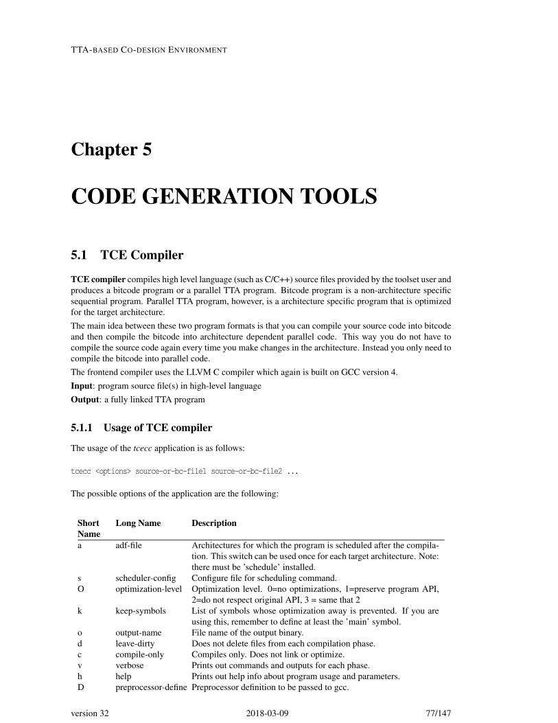
TTA-BASED CO-DESIGN ENVIRONMENT
Chapter 5
CODE GENERATION TOOLS
5.1 TCE Compiler
TCE compiler compiles high level language (such as C/C++) source files provided by the toolset user andproduces a bitcode program or a parallel TTA program. Bitcode program is a non-architecture specificsequential program. Parallel TTA program, however, is a architecture specific program that is optimizedfor the target architecture.The main idea between these two program formats is that you can compile your source code into bitcodeand then compile the bitcode into architecture dependent parallel code. This way you do not have tocompile the source code again every time you make changes in the architecture. Instead you only need tocompile the bitcode into parallel code.The frontend compiler uses the LLVM C compiler which again is built on GCC version 4.Input: program source file(s) in high-level languageOutput: a fully linked TTA program
5.1.1 Usage of TCE compiler
The usage of the tcecc application is as follows:
tcecc <options> source-or-bc-file1 source-or-bc-file2 ...
The possible options of the application are the following:
ShortName
Long Name Description
a adf-file Architectures for which the program is scheduled after the compila-tion. This switch can be used once for each target architecture. Note:there must be ’schedule’ installed.
s scheduler-config Configure file for scheduling command.O optimization-level Optimization level. 0=no optimizations, 1=preserve program API,
2=do not respect original API, 3 = same that 2k keep-symbols List of symbols whose optimization away is prevented. If you are
using this, remember to define at least the ’main’ symbol.o output-name File name of the output binary.d leave-dirty Does not delete files from each compilation phase.c compile-only Compiles only. Does not link or optimize.v verbose Prints out commands and outputs for each phase.h help Prints out help info about program usage and parameters.D preprocessor-define Preprocessor definition to be passed to gcc.
version 32 2018-03-09 77/147

TTA-based Co-design Environment v1.17 User Manual
I include-directory Include directory to be passed to gcc.L library-directory Passed to gcc.l library-link Passed to gcc.W warning Ignored.- scheduler-binary Scheduler binary to use instead of ’schedule’ in path.- extra-llc-flags Options passed to llc.- plugin-cache-dir Directory for cached llvm target plugins.- no-plugin-cache Do not cache generated llvm target plugins.- rebuild-plugin Rebuild plugin in the cache- clear-plugin-cache Clear plugin cache completely.
5.1.1.1 Examples of usage
Usage of tcecc quite alike to gcc, excluding that warning options are ignored.
If you wish to compile your source code into optimized bitcode the usage is:
tcecc -O2 -o myProg myProg.c
On the other hand if you already have an architecture definition file of the target processor you cancompile the source code directly to parallel program:
tcecc -O2 -a myProcessor.adf -o myProg.tpef myProg.c
To compile the bitcode program into parallel program use:
tcecc -a myProcessor.adf -o myProg.tpef myProg.bc
Or if you want to a different scheduling configuration than the default:
tcecc -s /path/to/mySchedulerConfiguration.conf -a myProcessor.adf -o myProg.tpefmyProg.bc
Tcecc also has a “leave dirty” flag -d which preserves the intermediate files created by the compiler. Aftercompilation is complete tcecc will tell you where to find these files (usually it is /tmp/tcecc-xxxxxx/). Forexample if you try to compile your C-code straight into a scheduled program and something goes wrongin scheduling you can find the bitcode program from the temp directory.
tcecc -d -O2 -a myProcessor.adf -o myProg.tpef myProg.c
After compilation you should see this kind of message:
Intermediate files left in build dir /tmp/tcecc-xxxxxx
where xxxxxx is a random pattern of characters.
If you only want to compile the source code without linking (and optimization) use -c flag. Output file isnamed after the source file with .o appendix if you do not define an output name with -o.
tcecc -c myProg.c
tcecc -c -o /another/path/myProg.o myProg.c
With tcecc you can explicitly define symbols you wish to preserve in the binary. This can be useful indebugging and profiling if the compiler removes needed function labels. Symbols are given in a commaseperated list.
tcecc -O2 -a myMach.adf -k main,foo,bar -o myProg.tpef myProg.c
Plugins
78/147 2018-03-09 version 32

TTA-BASED CO-DESIGN ENVIRONMENT
5.1.2 Custom operations
Tcecc compiler automatically defines macros for operations found from operation definition files inOSAL search paths and includes them when compiling your program.
The macros use the following format:
_TCE_<opName>(input1, ... , inputN, output1, ... , outputN);
where <name> is the operation name defined in OSAL. Number of input and output operands depends onthe operation.
There are also versions of the custom operation macros which can be used to explicitly target an functionunit (FU).
Usage of the “explicit-FU“ macros is as follows:
_TCEFU_<opName>(<fuName>, input1, ... , inputN, output1, ... , outputN);
where <fuName> is the name of the target function unit in ProDe.
There are also versions of the custom operation macros which can be used to target specific addressspace for operations that use memory. These may be need to be used for custom memory operations onarchitectures with multiple memory address spaces, as the address space information of a pointer may belost with the ordinary custom operation call.
_TCEAS_<opName>("#<as-numerical-id>", input1, ... , inputN, output1, ... , outputN);
or
_TCEAS_<opName>("<as-name>", input1, ... , inputN, output1, ... , outputN);
where <as-numerical-id> is the numerical id of the target address space, and <as-name> is the name ofthe target address space. This name is NOT necessaryly the same as the keyword in C code, this is thename visible in ProDE. Numerical id 0 is always where where the stack is located.
Examples of usage:
_TCE_MAC(a, b, c);_TCEFU_MAC("MAC1", a, b, c);_TCEAS_LDW("#1", a, b)_TCEAS_LDW("my_huge_global_addresspace", a, b)
5.1.3 Endianess Mode
Endianess mode property of the target architecture determines how the initialized data is layout into thedata memories and operation selections for accessing the memories by the compiler. In the table 5.2 islist of memory operations required by the compiler in the selected endianess mode.
The endianess mode is selected in ProDe’s Architecture Features... dialog (Edit -> Architecture Fea-tures...).
5.1.4 Known issues
1. Currently it is not possible to simulate a bitcode format program. But the advantage of bitcodesimulation is quite non-existent because the bitcode does not even contain the final basic blocksthat the architecture dependent program has.
version 32 2018-03-09 79/147

TTA-based Co-design Environment v1.17 User Manual
Big endian Little endianldq ld8ldqu ldu8ldh ld16ldhu ldu16ldw ld32stq st8sth st16stw st32
Table 5.2: The required memory operations in the selected endianess modes.
5.2 Binary Encoding Map Generator (BEMGenerator)
Binary Encoding Map Generator (BEMGenerator) creates a file that describes how to encode TTAinstructions for a given target processor into bit patterns that make up the executable bit image of theprogram (before compression, if used).
Input: ADF
Output: BEM
5.2.1 Usage
The usage of BEMgenerator is the following:
createbem -o outName.bem myProcessor.adf
5.3 Parallel Assembler and Disassembler
TCE Assembler compiles parallel TTA assembly programs to a TPEF binary. The Disassembler pro-vides a textual disassembly of parallel TTA programs. Both tools can be executed only from the commandline.
Assembler Input: program source file in the TTA parallel assembler language and an ADF
Output: parallel TPEF
Disassembler Input: parallel TPEF
Output: textual disassembly of the program
Rest of this section describes the textual appearance of TTA programs, that is, how a TTA program shouldbe disassembled. The same textual format is accepted and assembled into a TTA program.
5.3.1 Usage of Disassembler
The usage of the tcedisasm application is as follows:
tcedisasm <options> adffile tpeffile
The adffile is the ADF file.The tpeffile is the parallel TPEF file.
The possible options of the application are as follows:
80/147 2018-03-09 version 32

TTA-BASED CO-DESIGN ENVIRONMENT
ShortName
Long Name Description
o outputfile The name of the output file.h help Prints out help info about program usage and parameters.
The application disassembles given parallel TPEF file according to given ADF file. Program output isdirected to standard output stream if specific output file is not specified. The output is TTA parallelassembler language.The program output can then be used as an input for the assembler program tceasm.The options can be given either using the short name or long name. If short name is used, a hyphen (-)prefix must be used. For example -o followed by the name of the output file. If the long name is used, adouble hyphen (- -) prefix must be used, respectively.
5.3.1.1 An example of the usage
The following example generates a disassemble of a parallel TPEF in the file add4_schedule.tpef andwrites the output to a file named output_dis.asm.
tcedisasm -o output_dis.asm add4_supported.adf add4_schedule.tpef
5.3.2 Usage of Assembler
The usage of the tceasm application is as follows:
tceasm <options> adffile assemblerfile
The adffile is the ADF file.The assemblerfile is the program source file in TTA parallel assembler language.
The possible options of the application are as follows:
ShortName
Long Name Description
o outputfile The name of the output file.q quiet Do Not print warnings.h help Help info about program usage and parameters.
The application creates a TPEF binary file from given assembler file. Program output is written to a filespecified by outputfile parameter. If parameter is not given, the name of the output file will be the basename of the given assembler file concatenated with .tpef.The options can be given either using the short name or long name. If short name is used, a hyphen (-)prefix must be used. For example -o followed by the name of the ouput file. If the long name is used, adouble hyphen (- -) prefix must be used, respectively.
5.3.2.1 An example of the usage
The following example generates a TPEF binary file named program.tpef.
tceasm add4_schedule.adf program.asm
5.3.3 Memory Areas
A TTA assembly file consists of several memory areas. Each area specifies the contents (instructions ordata) of part of an independently addressed memory (or address space). There are two kinds of memory
version 32 2018-03-09 81/147

TTA-based Co-design Environment v1.17 User Manual
areas: code areas and data areas. Code areas begin a section of the file that defines TTA instructions. Dataareas begin a section that define groups of memory locations (each group is collectively termed “mem-ory chunk” in this context) and reserve them to variables. By declaring data labels (see Section 5.3.7),variables can be referred to using a name instead of their address.Memory areas are introduced by a header, which defines the type of area and its properties. The headeris followed by several logical lines (described in Section 5.3.4), each declaring a TTA instruction or amemory chunk. The end of an area in the assembly file is not marked. Simply, a memory area terminateswhen the header of another memory area or the end of the assembly file is encountered.The memory area header has one of the following formats:
\ttCODE [\parm{start}] ;\\DATA \parm{name} [\parm{start}] ;
A code area begins the declaration of TTA instructions that occupy a segment of the instruction memory.A data area begins the declaration of memory chunks reserved to data structures and variables.A TTA program can work with several independently addressed data memories. The locations of differentmemories belong to different address spaces. The name parameter defines the address space a memoryarea belongs to. The code area declaration does not have a name parameter, because TTA programssupport only one address space for instruction memory, so its name is redundant.The start parameter defines the starting address of the area being declared within its address space. Thestart address can and usually is omitted. When omitted, the assembler will compute the start address andarrange different memory area declarations that refer to the same address space. The way the start addressis computed is left to the assembler, which must follow only two rules:
1. If a memory area declaration for a given address space appears before another declaration for thesame address space, it is assigned a lower address.
2. The start address of a memory area declaration is at least equal to the size of the previous areadeclared in the same address space plus its start address.
The second rule guarantees that the assembler reserves enough memory for an area to contain all the(chunk or instruction) declarations in it.
5.3.4 General Line Format
The body of memory areas consists of logical lines. Each line can span one or more physical lines ofthe text. Conversely, multiple logical lines can appear in a single physical lines. All logical lines areterminated by a semicolon ‘;’.The format of logical lines is free. Any number of whitespace characters (tabs, blanks and newlines) canappear between any two tokens in a line. Whitespace is ignored and is only useful to improve readability.See Section 5.3.14 for suggestions about formatting style and use of whitespaces.Comments start with a hash character (‘#’) and end at the end of the physical line. Comments are ignoredby the syntax. A line that contains only a comment (and possibly whitespaces before the hash character)is completely removed before interpreting the program.
5.3.5 Allowed characters
Names (labels, procedures, function units etc.) used in assembly code must obey the following format:
[a-zA-Z_][a-zA-z0-9_]*
Basically this means is that a name must begin with a letter from range a-z or A-Z or with an underscore.After the first character numbers can also be used.Upper case and lower case letters are treated as different characters. For example labels main: and Main:are both unique.
82/147 2018-03-09 version 32

TTA-BASED CO-DESIGN ENVIRONMENT
5.3.6 Literals
Literals are expressions that represent constant values. There are two classes of literals: numeric literalsand strings.
Numeric literals. A numeric literal is a numeral in a positional system. The base of the system (orradix) can be decimal, hexadecimal or binary. Hexadecimal numbers are prefixed with ‘0x’, binarynumbers are prefixed with ‘0b’. Numbers in base 10 do not have a prefix. Floating-point numbers canonly have decimal base.Example: Numeric literals.
0x56F05A71160830b1101100100101010011001117.759308e+55
The first three literals are interpreted as integer numbers expressed in base, respectively, 16, 10 and 2. Anall-digit literal string starting with ‘0’ digit is interpreted as a decimal number, not as an octal number,as is customary in many high level languages.1 The last two literals are interpreted as floating pointnumbers. Unlike integer literals, floating-point literals can appear only in initialisation sequences of datadeclarations (see Section 5.3.8 for details).
String literals. A string literal consists of a string of characters. The the numeric values stored in thememory chunk initialised by a string literal depend on the character encoding of the host machine. The EXTENSION: charset di-
rectiveuse of string literals makes the assembly program less portable.Literals are defined as sequences of characters enclosed in double (") or single (’) quotes. A literal canbe split into multiple quoted strings of characters. All strings are concatenated to form a single sequenceof characters.Double quotes can be used to escape single quotes and vice versa. To escape a string that contains both,the declaration must be split into multiple strings.Example: String literals. The following literals all declare the same string Can’t open file "%1" .
"Can’t open file" ’"%1"’’Can’ "’" ’t open file "%1"’"Can’t open" ’ file "%1"’
String literals can appear only in initialisation sequences of data declarations (see Section 5.3.8 for de-tails).
Size, encoding and layout of string literals. By default, the size (number of MAU’s) of the valuedefined by a string literal is equal to the number of characters. If one MAU is wider than the characterencoding, then the value stored in the MAU is padded with zeroes. The position of the padding bitsdepends on the byte-order of the target architecture: most significant if “big endian”, least significant if“little endian”.If one character does not fit in a singe MAU, then each character is encoded in ⌈m/n⌉ MAU’s, where n isthe MAU’s bit width and m is the number of bits taken by a character.When necessary (for example, to avoid wasting bits), it is possible to specify how many characters arepacked in one MAU or, vice versa, how many MAU’s are taken to encode one character. The size specifierfor characters is prefixed to a quoted string and consists of a number followed by a semicolon.If n > m, the prefixed number specifies the number of characters packed in a single MAU. For example,if one MAU is 32 bits long and a character takes 8 bits, then the size specifier in
1 This notation for octal literals has been deprecated.
version 32 2018-03-09 83/147

TTA-based Co-design Environment v1.17 User Manual
4:"My string"
means: pack 4 characters in one MAU. The size specifier cannot be greater than ⌈n/m⌉. The size ‘1’ isequivalent to the default.If m > n, the prefixed number specifies the number of adjacent MAU’s used to encode one character. Forexample, if MAU’s are 8-bit long and one character takes 16 bits, then the same size specifier means:reserve 4 MAU’s to encode a single character. In this case, a 16-bit character is encoded in 32 bits, andpadding occurs as described above. The size of the specifier in this case cannot be smaller than ⌈n/m⌉,which is the default value when the size is not specified explicitly.
5.3.7 Labels
A label is a name that can be used in lieu of a memory address. Labels “decorate” data or instructionaddresses and can be used to refer to, respectively, the address of a data structure or an instruction. Theaddress space of a label does not need to be specified explicitly, because it is implied by the memory areadeclaration block the label belongs to.A label declaration consists of a name string followed by a colon:
\tt\parm{label-name}:
Only a restricted set of characters can appear in label names. See Section 5.3.5 for details.A label must always appear at the beginning of a logical line and must be followed by a normal linedeclaration (see Sections 5.3.8, 5.3.9 for details). Only whitespace or another label can precede a label.Label declarations always refer to the address of the following memory location, which is the start locationof the element (data chunk or a TTA instruction) specified by the line.Labels can be used instead of the address literal they represent in data definitions and instruction defini-tions. They are referred to simply by their name (without the colon), as in the following examples:
# label reference inside a code area (as immediate)aLabel -> r5 ;
# label reference inside a data area (as initialisation value)DA 4 aLabel ;
5.3.8 Data Line
A data line consists of a directive that reserves a chunk of memory (expressed as an integer number ofminimum addressable units) for a data structure used by the TTA program:
\ttDA \parm{size} [\parm{init-chunk-1} \parm{init-chunk-2} \ldots] ;
The keyword ‘DA’ (Data Area) introduces the declaration of a memory chunk. The parameter size givesthe size of the memory chunk in MAU’s of the address space of the memory area.Memory chunks, by default, are initialised with zeroes. The memory chunk can also be initialised ex-plicitly. In this case, size is followed by a number of literals (described in Section 5.3.6) or labels (Sec-tion 5.3.7) that represent initialisation values. An initialisation value represents a constant integer numberand takes always an integer number of MAU’s.
Size of the initialisation values. The size of an initialisation value can be given by prepending the size(in MAU’s) followed by a semicolon to the initialisation value. If not defined explicitly, the size of theinitialisation values is computed by means of a number of rules. If the declaration contains only oneinitialisation value, then the numeric value is extended to size, otherwise, the rules are more complex anddepend on the type of initialisation value.
84/147 2018-03-09 version 32

TTA-BASED CO-DESIGN ENVIRONMENT
1. If the initialisation value is a numeric literal expressed in base 10, then it is extended to size MAU’s.
2. If the initialisation value is a numeric literal expressed in base 2 or 16, then its size is extended tothe minimum number of MAU’s necessary to represents all its digits, even if the most significantdigits are zeroes.
3. If the initialisation value is a label, then it is extended to size MAU’s.
Extension sign. Decimal literals are sign-extended. Binary, hexadecimal and string literal values arezero-extended. Also the initialisation values represented by labels are always zero-extended.
Partial Initialisation. If the combined size of the initialisation values (computed or specified explicitly,it does not matter) is smaller than the size declared by the ‘DA’ directive, then the remaining MAU’s areinitialised with zeroes.Example: Padding of single initialisation elements. Given an 8-bit MAU, the following declarations:
DA 2 0xBB ; # equivalent to 2:0xBBDA 2 0b110001 ; # 0x31 (padded with 2 zero bits)DA 2 -13 ;
define 2-MAU initialisation values: 0x00BB, 0x0031, and 0xFFF3, respectively.Example: Padding of of multi-element initialisation lists. The following declarations:
DA 4 0x00A8 0x11;DA 4 0b0000000010100100 0x11 ;
are equivalent and force the size of the first initialisation value in each list to 16 bits (2 MAU’s) even ifthe integer expressed by the declarations take less bits. The 4-MAU memory chunk is initialised, in bothdeclarations, with the number 0x00A81100. Another way to force the number of MAU’s taken by eachinitialisation value is to specify it explicitly. The following declarations are equivalent to the declarationsabove:
DA 4 2:0xA8 0x11;DA 4 2:0b10100100 0x11;
Finally, the following declarations:
DA 2 1:0xA8 0x11;DA 2 1:0b10100100 0x11;
define a memory chunk initialised with 0xA8110000. The initialisation value (in case of the binary literal,after padding to MAU bit width) defines only the first MAU.When labels appear in initialisation sequences consisting of multiple elements, the size of the label ad-dress stored must be specified explicitly.Example. Initialisation with Labels. The following declaration initialises a 6-MAU data structure wherethe first 2 MAU’s contain characters ‘A’ and ‘C’, respectively, and the following 4 MAU’s contain twoaddresses. The addresses, in this target architecture, take 2 MAU’s.
DA 6 0x41 0x43 2:nextPointer 2:prevPointer ;
5.3.9 Code Line
A code line defines a TTA instruction and consists of a comma-separated, fixed sequence of bus slots. Abus slot in any given cycle can either program a data transport or encode part of a long immediate andprogram the action of writing it to a destination (immediate) register for later use.2
2 The action of actually writing the long immediate to a destination register is encoded in a dedicated instruction field, and isnot repeated in each move slot that encodes part of the long immediate. This detail is irrelevant from the point of view of programspecification. Although the syntax is slightly redundant, because it repeats the destination register in every slot that encodes a pieceof a long immediate, it is chosen because it is simple and avoids any chance of ambiguity.
version 32 2018-03-09 85/147

TTA-based Co-design Environment v1.17 User Manual
A special case of code line that defines an empty TTA instruction. This line contains only three dotsseparated by one or more white spaces:
. . . ; # completely empty TTA instruction
A special case of move slot is the empty move slot. An empty move slot does not program any datatransport nor encodes bits of a long immediate. A special token, consisting of three dots represents anempty move slot. Thus, for a three-bus TTA processor, the following code line represents an emptyinstruction:
... , ... , ... ; # completely empty TTA instruction
5.3.10 Long Immediate Chunk
When a move slot encodes part of a long immediate, its declaration is surrounded by square brackets andhas the following format:
\tt\parm{destination}=\parm{value}
where destination is a valid register specifier and value is a literal or a label that gives the value ofthe immediate. The only valid register specifiers are those that represent a register that belongs to animmediate unit. See section 5.3.12 for details on register specifiers.
When the bits of a long immediate occupy more than one move slot, the format of the immediate dec-laration is slightly more complex. In this case, the value of the immediate (whether literal or label) isdeclared in one and only one of the slots (it does not matter which one). The other slots contain only thedestination register specifier.
5.3.11 Data Transport
A data transport consists of one optional part (a guard expression) and two mandatory parts (a source anda destination). All three can contain an port or register specifier, described in Section 5.3.12.
The guard expression consists of a single-character that represents the invert flag followed by a sourceregister specifier. The invert flag is expressed as follows:
1. Single-character token ‘!’: the result of the guard expression evaluates to zero if the source value isnonzero, and evaluates to one if the source value is equal to zero.
2. Single-character token ‘?’: the result of the guard expression evaluates to zero if the source valueis zero, and evaluates to one if the source value is not zero.
The move source specifier can be either a register and port specifier or an in-line immediate. Register andport specifiers can be GPR’s, FU output ports, long immediate registers, bridge registers. The format ofall these is specified in Section 5.3.12. The in-line immediate represents an integer constant and can bedefined as a literal or as a label. In the latter case, the in-line immediate can be followed by an equal signand a literal corresponding to the value of the label. The value of the labels is more likely to be shownas a result of disassembling an existing program than in user input code, since users can demand dataallocation and address resolution to the assembler.
Example: Label with value. The following move copies the label ‘LAB’, which represents the address0x051F0, to a GPR:
LAB=0x051F0 -> r.4
The move destination consists of a register and port specifier of two types: either GPR’s or FU inputports.
86/147 2018-03-09 version 32

TTA-BASED CO-DESIGN ENVIRONMENT
5.3.12 Register Port Specifier
Any register or port of a TTA processor that can appear as a move or guard source, or as a move destinationis identified and referred to by means of a string. There are different types of register port specifiers:
1. General-purpose register.
2. Function unit port.
3. Immediate register.
4. Bridge register.
GPR’s are specified with a string of the following format:
\tt\parm{reg-file}[.\parm{port}].\parm{index}
where reg-file is the name of the register file, port, which can be omitted, is the name of the port through DISCUSS: pending ??
which the register is accessed, and index is the address of the register within its register file.
Function unit input and output ports are specified with a string of the following format:
\tt\parm{function-unit}.\parm{port}.[\parm{operation}]
where function-unit is the name of the function unit, port is the name of the port through which the reg-ister is accessed, and operation, which is required only for opcode-setting ports, identifies the operationperformed as a side effect of the transport. It is not an error to specify operation also for ports that donot set the opcode. Although it does not represent any real information encoded in the TTA program, thiscould improve the readability of the program.
Immediate registers are specified with a string if the following format:
\tt\parm{imm-unit}[.\parm{port}].\parm{index}
where imm-unit is the name of the immediate unit, port, which can be omitted, is the name of the port DISCUSS: pending ??
through which the register is accessed, and index is the address of the register within its unit.
Since any bus can be connected to at most two busses through bridges, it is not necessary to specify bridgeregisters explicitly. Instead, the string that identifies a bridge register can only take one of two values:‘{prev}’ or ‘{next}’. These strings identify the bus whose value in previous cycle is stored in the registeritself. A bus is identified by ‘{prev}’ if it is programmed by a bus slot that precedes the bus slot that readsthe bridge register. Conversely, if the bus is identified by ‘{next}’, then it is programmed by a bus slotthat follows the bus slots that reads the bridge register. In either case, the source bus slot must be adjacentto the bus slot that contains the moves that reads the bridge register.
Example: possible register and port specifiers.
\begin{tabular}{lp{0.75\textwidth}}\texttt{IA.0} & immediate unit ‘IA’, register with index 0\\\texttt{RFA.5} & register file ‘RFA’, register with index 5\\\texttt{U.s.add} & port ‘s’ of function unit ‘U’, opcode for operation‘add’\\\verb|{|\texttt{prev}\verb|}| & bridge register that contains the value onthe
bus programmed by the previous bus slot in previouscycle\\\end{tabular}
version 32 2018-03-09 87/147

TTA-based Co-design Environment v1.17 User Manual
Alternative syntax of function unit sources and destinations. Most clients, especially user interfaces,may find direct references to function unit ports inconvenient. For this reason, an alternative syntax issupported for input and output ports of function units:
\tt\parm{function-unit}.\parm{operation}.\parm{index}
where function-unit is the name of the function unit, operation identifies the operation performed as a sideeffect of the transport and index is a number in the range [1,n], where n is the total number of inputs andoutputs of the operation. The operation input and output, indirectly, identifies also the FU input or outputand the port accessed. Contrary to the base syntax, which is requires the operation name only for opcode-setting ports, this alternative syntax makes the operation name not optional. The main advantage of thissyntax is that is makes the code easier to read, because it removes the need to know what is the operationinput or output bound to a port, because. The main drawback is an amount of (harmless) “fuzziness” andinconsistency, because it forces the user to define an operation for ports that do not set the opcode, evenin cases where the operand is shared between two different operations. For example, suppose that theoperand ‘1’ of operations ‘add’ and ‘mul’ is bound to a port that does not set the opcode and its value isshared between an ‘add’ and a ‘mul’:
r1 -> U1.add.1, r2 -> U1.add.2;U1.add.3 -> r3, r4 -> U1.mul.2;U1.mul.3 -> r5
it looks as if the shared move belonged only to ‘add’. One could have also written, correctly but lessclearly:
r1 -> U1.mul.1, r2 -> U1.add.2;# same code follows
or even, assuming that operation ‘sub’ is also supported by the same unit and its operand ‘1’ is bound tothe same port:
r1 -> U1.sub.1, r2 -> U1.add.2;# same code follows
This alternative syntax is the only one permitted for TTA moves where operations are not assigned to afunction unit of the target machine.
5.3.13 Assembler Command Directives
Command directives do not specify any code or data, but change the way the assembler treats (part of) thecode or data declared in the assembly program. A command directive is introduced by a colon followedby the name string that identifies it, and must appear at the beginning of a new logical line (possibly withwhitespace before).
The assembler recognises the following directives.
procedure The ‘:procedure ’ directive defines the starting point of a new procedure. This directive isfollowed by one mandatory parameter: the name of the procedure. Procedure directives should appearonly in code areas. The procedure directive defines also, implicitly, the end of procedure declared bythe previous ‘:procedure’ directive. If the first code section of the assembly program contains any codebefore a procedure directive, the code is assumed to be part of a nameless procedure. Code in followingcode areas that precede any procedure directive is considered part of the last procedure declared in one ofthe previous code areas.
Example: declaration of a procedure.
88/147 2018-03-09 version 32

TTA-BASED CO-DESIGN ENVIRONMENT
CODE ;:procedure Foo ;Foo:
r5 -> r6 , ... ;. . . ;... , r7 -> add.1 ;
In this example, a procedure called ‘Foo’ is declared and a code label with the same name is declared atthe procedure start point. The code label could be given any name, or could be placed elsewhere in thesame procedure. In this case, the code label ‘Foo’ marks the first instruction of procedure ‘Foo’.
global The ‘:global directive declares that a given label is globally visible, that is, it could be linkedand resolved with external code. This directive is followed by one mandatory parameter: the name of thelabel. The label must be defined in the same assembly file. The label may belong to the data or the codesection, indifferently.
extern The ‘:extern directive declares that a given label is globally visible and must be resolved anexternal definition. This directive is followed by one mandatory parameter: the name of the label. Thelabel must not be defined in the assembly file.There can be only one label with any given name that is declared global or external.Example: declaration of undefined and defined global labels.
DATA dmem 0x540;aVar:
DA 4 ;:global aVar ;:extern budVar ;
In this example, ‘aVar’ is declared to have global linkage scope (that is, it may be used to resolve refer-ences from other object files, once the assembly is assembled). Also ‘budVar’ is declared to have globallinkage, but in this case the program does not define a data or code label with that name anywhere, andthe symbol must be resolved with a definition in an external file.
5.3.14 Assembly Format Style
This section describes a number of nonbinding guidelines that add to the assembly syntax specificationand are meant to improve programs’ readability.
Whitespaces. Although the format of the assembly is completely free-form, tabs, whitespaces and newlines can be used to improve the assembly layout and the readability. The following rules are suggested:
1. Separate the following tokens with at least one whitespace character:
(a) Label declaration ‘name:’ and first move or ‘DA’ directive.(b) Moves of an instruction and commas.(c) Move source and destination and the ‘->’ or ‘<-’ token.
2. Do not separate the following tokens with whitespaces:
(a) Long immediate chunk declaration and the surrounding brackets.(b) Label and, literal and the ‘=’ token in between.(c) Any part of a register specifier (unit, port, operation, index) and the ‘.’ separator token.(d) Register specifier, label or literal and the ‘=’ in between.(e) Invert flag mark (‘!’ or ‘?’) and the register specifier of a guard expression.(f) Initialisation chunk, the number of MAU’s it takes and the ‘:’ token in between.(g) Colon ‘:’ and the nearby label or directive name.
version 32 2018-03-09 89/147

TTA-based Co-design Environment v1.17 User Manual
End of Line. The length of physical lines accepted is only limited by client implementation. Linesup to 1024 characters must be supported by any implementation that complies with these specifications.However, it is a good rule, to improve readability, that physical line should not exceed the usual line lengthof 80 or 120 characters. If a TTA instruction or a data declaration does not fit in the standard length, thelogical line should be split into multiple physical lines. The physical lines following the first piece of alogical line can be indented at the same column or more to the right. In case of data declarations, the lineis split between two literals that form an initialisation data sequence. In case of TTA instructions, logicallines should never be split after a token of type ‘X’ if it is recommended that no whitespace should follow‘X’ tokens. To improve readability, TTA instructions should be split only past the comma that separatestwo move slots:
# good line breakingr2 -> U.sub.1 , [i1=var] , r3 -> U.sub.2 , i1 -> L.ld.1 , [i1] ,0 -> U.eq.2 ;
# bad line breakingr2 -> U.sub.1 , [i1=var] , r3 -> U.sub.2 , i1 -> L.ld.1 , [i1] , 0 ->U.eq.2 ;
# really bad line breakingr2 -> U.sub.1 , [i1=var] , r3 -> U.sub.2 , i1 -> L.ld.1 , [i1] , 0 -> U.eq.2 ;
Tabulation. The following rules can be taken as starting point for a rather orderly layout of the assemblytext, which resembles the layout of traditional assembly languages:
1. The first n characters of the assembly lines are reserved to labels. Instruction or data declarationsare always indented by n characters.
2. Labels appear in the same physical line of the instruction or data declaration they refer to. Labelsare no more than n−2 characters long.
This layout is particularly clean when the TTA instructions contain few bus slots and when multiple labelsfor the same data chunk or instruction do not occur.Example: Assembly layout style best suited target architectures with few busses.
DATA DMEMvar: DA 4;
CODElab_A: spr -> U.add.1 , 55 -> U.add.2 , spr -> r12 ;
[i0=0x7F] , U.add.3 -> spr , i0 -> r2 ;loop_1: r2 -> U.sub.1 , r3 -> U.sub.2 , var -> L.ld.1 ;
r2 -> U.eq.1 , U.sub.3 -> r2 , 0 -> U.eq.2 ;?U.eq.3 loop_1 -> C.jump.1 , L.ld.2 -> U.and.2 ;0x1F -> U.and.1 , ... , ... ;... , U.and.3 -> r8 , ... ;
An alternative layout of the assembly text is the following:
1. Instruction and data declarations are always indented by n characters.
2. Each label declaration appears in a separate physical line of the instruction or data declaration theyrefer to, and starts from column 0.
This layout could be preferable when the TTA instructions contain so many bus slots that the logical lineis usually split into multiple physical lines, because it separates more clearly the code before and after a
90/147 2018-03-09 version 32

TTA-BASED CO-DESIGN ENVIRONMENT
label (which usually marks also a basic block entry point). In addition, this layout looks better when aninstruction or data declaration has multiple labels and when the label name is long.
Example: Assembly layout style best suited targets with many busses.
DATA DMEMvar:
DA 4;
CODEa_long_label_name:
spr -> U.add.1 , 55 -> U.add.2 , spr -> r12 , [i0=0x7F], i0 -> r2,... ;... , U.add.3 -> spr , ... , ... , ... , ... ;
loop_1:r2 -> U.sub.1 , [i1=var] , r3 -> U.sub.2 , i1 -> L.ld.1 , [i1] ,0 -> U.eq.2 ;r2 -> U.eq.1 , U.sub.3 -> r2 , ... , ?U.eq.3 loop_1 -> C.jump.1 ,0x1F -> U.and.1 , ... ;L.ld.2 -> U.and.2 , ... , ... , ... , ... , ... ;... , ... , ... , U.and.3 -> r8 , ... , ... ;
This example of assembly code is exactly equivalent to the code of previous example, except that theaddress of ‘var’ data chunk (a 4-MAU word) is encoded in a long immediate and takes 2 move slots.
Layout of Memory Area Declarations. It is preferable to subdivide the contents of memories intoseveral memory area declarations and to group near each other area declarations of different addressspaces that are related to each other. This underlines the relation between data and code. The alternative,a single area for each address space, mixes together all data and all procedures of a program.
Mixing Alternative Syntaxes. It is preferable to not mix alternative styles or even syntaxes, althoughany client that works with the assembly language is expected to deal with syntax variants.
5.3.15 Error Conditions
This section describes all the possible logical errors that can occur while assembling a TTA program.
Address Width Overflow in Initialisation. A label is used as initialisation value of a data declaration,and the label address computed by the assembler exceeds the number of MAU’s in the data declarationthat must be initialised.
Address Width Overflow in Long Immediate. A label is used as initialisation value of a long imme-diate declaration, and the label address computed by the assembler exceeds total width of the move slotsthat encode the immediate, when concatenated together.
Address Width Overflow in In-line Immediate. A label is used as initialisation value of an in-lineimmediate, and the label address computed by the assembler exceeds width of source field that encodesthe immediate.
Unspecified Long Immediate Value. A long immediate is defined, but none of the move slots thatencode its bits defines the immediate value.
version 32 2018-03-09 91/147

TTA-based Co-design Environment v1.17 User Manual
Multiply Defined Long Immediate Value. More than one of the move slots that contain the bits of along immediate defines the immediate value.3
Overlapping Memory Areas. The start address specified in the header of two memory area declara-tions is such that, once computed the sizes of each memory area, there is an overlapping.
Multiple Global Symbols with Same Name. A ‘:global’ directive declares a symbol with given nameas globally visible, but multiple labels with given name are declared in the program.
Unknown Command Directive. A command directive has been found that is not one of the directivessupported by the assembler.
Misplaced Procedure Directive. A ‘:procedure’ directive appears inside a data area declaration block.
Procedure Directive Past End of Code. A ‘:procedure’ directive appears after the last code line in theprogram.
Label Past End of Area. A label has been declared immediately before an area header or at the end ofthe assembly program. Labels must be followed by a code line or a data line.
Character Size Specifier too Big. A size specified for the characters of a string literal is greater thanthe maximum number of characters that can fit in one MAU.
Character Size Specifier too Small. A size specified for the characters of a string literal is smaller thanthe minimum number of MAU’s necessary to encode one character.
Illegal Characters in Quoted String. A quoted string cannot contain non-printable characters (that is,characters that cannot be printed in the host encoding) and end-of-line characters.
5.3.16 Warning Conditions
This section describes all conditions of target architecture or assembly syntax for which the client shouldissue an optional warning to prepare users for potential errors or problematic conditions.
Equally Named Register File and Function Unit. A register file and a function unit of the targetarchitecture have the same name. This is one of the conditions for the activation of the disambiguationrule.
Port with the Name of an Operation. A register file or a function unit port are identified by a stringname that is also a name of a valid operation supported by the target architecture. The first condition(port of register file) is more serious, because it may require triggering a disambiguation rule. The secondcondition (FU port) is not ambiguous, but is confusing and ugly. The second condition may be more orless severe depending, respectively, whether the operation with the same name is supported by the sameFU or by another FU.
Code without Procedure. The first code area of the program begins with code lines before the first‘:procedure’ directive. A nameless procedure with local visibility is automatically created by the assem-bler.
3 If the values are identical in every move slot, then the client could issue a warning rather than a critical error.
92/147 2018-03-09 version 32

TTA-BASED CO-DESIGN ENVIRONMENT
Procedure Spanning Multiple Code Areas. A code area contains code line before the first ‘:procedure’directive, but it is not the first code area declared in the code. The code at the beginning of the area isattached to the procedure declared by the last ‘:procedure’ directive.
Empty Quoted String. Empty quoted strings are ignored.
5.3.17 Disambiguation Rules
Certain syntactic structures may be assigned different and (in principle) equally valid interpretations.In these cases, a disambiguation rule assigns priority to one of the two interpretation. Grammaticallyambiguous assembly code should be avoided. Clients that operate on TTA assembly syntax should issuea warning whenever a disambiguation rule is employed.
Disambiguation of GPR and FU terms. When a GPR term includes also the RF port specifier, it canbe interpreted also as a function unit input or output.Normally, the names of units, ports and operation rule out one of the two interpretations. Ambiguity canonly occur only if:
1. The target architecture contains a RF and a FU with identical name.
2. One of the RF ports has a name identical to one of the operations supported by the FU that has thesame name of the RF. PENDING: disambigua-
tion of unscheduled TTAcode ??Ambiguity is resolved in favour of the GPR interpretation. No condition applies to the indices (register
index or operation input or output index). The first interpretation is chosen even when it results in asemantic error (an index out of range) whereas the other interpretation would be valid.Example. Disambiguation rule. The following move is interpreted as a move that writes the constant55 to the register with index 2 of register file ‘xx’ through port ‘yy’. If there exists an FU called ‘xx’that supports an operation ‘yy’ which has an input with index 2, this interpretation of the move is neverpossible.
55 -> xx.yy.2
Even if the disambiguation rule is not triggered, clients should warn when the target architecture satisfiesone of the conditions above (or a similar condition). See Section 5.3.16 for a description of this and otherconditions for which a warning should be issued.
Disambiguation of variables and operation terms. In unscheduled code, operation terms cannot beconfused with variables. The special RF names ‘r’, ‘f’ and ‘b’ are reserved, respectively, to integer,floating-point and Boolean register files of the universal machine. The assembler does not allow anyoperation to have one of these names. PENDING: disam-
biguation of mixed TTAcode ??Example. Unambiguous move term accessing a variable. The following move is interpreted as “copy
constant 55 to variable with index 2 of variable pool ‘r”’. There cannot exist an operation ‘r’, so theinterpretation of the move destination as operation term is impossible.
55 -> r.2
Disambiguation of Register File and Immediate Unit names Assembler syntax does not differentiateunit names of immediate units from unit names of register files. The same register specifier of a movesource
x.2 -> alu.add.1
can represents a GPR or an immediate register depending on whether ‘x’ is an RF or a IU.In this case the GPR interpretation is always preferred over the IU interpretation. However using the samenaming for IUs and GPRs restricts severely the programmability of target machine and is not encouraged.
version 32 2018-03-09 93/147

TTA-based Co-design Environment v1.17 User Manual
5.4 Program Image Generator (PIG)
Program Image Generator (PIG) generates the bit image which can be uploaded to the target machine’smemory for execution. Compression can be applied to the instruction memory image by means of in-struction compression algorithm plugins.Input: TPEF, BEM, ADFOutput: program bit image in alternative formats
5.4.1 Usage
The usage of the generatebits application is as follows:
generatebits <options> ADF
The possible options of the application are as follows:
ShortName
Long Name Description
b bem The binary encoding map file.c compressor Name of the code compressor plugin file.u compressorparam Parameter to the code compressor in form ’name=value’.d dataimages Creates data images.g decompressor Generates a decompressor block.o diformat The output format of data image(s) (’ascii’, ’array’, ’mif’ or ’binary’). Default
is ’ascii’.w dmemwidthinmaus Width of data memory in MAUs. Default is 1.x hdl-dir Directory root where are the ProGe generated HDL files generated by ProGe.
If given, PIG will write imem_mau_pkg and compressor in that directory. Oth-erwise they are written to cwd.
f piformat Determines the output format of the program image and data images. Valuemay be ’ascii’, ’binary’ or ’mif’.
s showcompressors Shows the compressor plugin descriptions.p program The TPEF program file(s).v verbose Display extra information during image creation: total immediates, different
immediate values, instr. addresses, data addresses, full instruction NOPs andconsecutive full instr. NOP groups.
The application prints the program image to the standard output stream. It can be easily forwarded to afile, if wanted. The data images are generated to separate files, one for each address space. Names of thefiles are determined by the name of the address space and the suffix is .img. The files are generated to thedirectory in which the application is executed.The binary encoding map input parameter may be omitted. If so, the BEM to be used is generatedautomatically. The BEM is used in the intermediate format of the program image, before it is compressedby the code compressor plugin. However, if no code compression is applied, the program image outputmatches the format defined in the BEM.The options can be given either using the short name or long name. If short name is used, a hyphen (-)prefix must be used. For example -a followed by the name of the ADF file. If the long name is used, adouble hyphen (- -) prefix must be used, respectively.
5.4.1.1 An example of the usage
The following example generates a program image and data images of the address spaces in ASCII formatwithout code compression.
generatebits -b encodings.bem -p program.tpef -f ascii -d machine.adf
94/147 2018-03-09 version 32

TTA-BASED CO-DESIGN ENVIRONMENT
5.4.2 Dictionary Compressor
TCE toolset includes two different code compressors: ’InstructionDictionary’ compressor and ’MoveS-lotDictionary’ compressor. It is also possible to create new code compressors.
How these compressors work is that they analyze program’s instruction memory and create a compressedinstruction memory image. In order to use the compressed image the compressor also creates a decom-pressor module which replaces the default decompressor in the instruction decoder unit of a processor.
You can list the available compressor and their descriptions with
generatebits -s processor.adf
5.4.2.1 Instruction Dictionary compressor
Instruction dictionary compressor analyzes a program and creates a look up table of all the unique instruc-tions. Compressed instruction image then consists of indices to the created look up table. Decompressormodule includes the look up table and it outputs the uncompressed instruction defined by the input index.
Here is an example how to use the instruction dictionary compressor:
generatebits -c InstructionDictionary.so -g -p program.tpef processor.adf
Command creates the compressed instruction memory image ’program.img’ and ’imem_mau_pkg.vhdl’using InstructionDictionary.so plugin defined with the -c parameter. As the command also has -g param-eter compressor creates the ’decompressor.vhdl’ file which defines the decompressor unit.
You can also give the existing proge-output directory (in this case processor_files) to generatebits:
generatebits -c InstructionDictionary.so -g -p program.tpef -x processor_files processor.adf
Now PIG will automatically write the ’imem_mau_pkg.vhdl’ and ’decompressor.vhdl’ to the right placesin processor_files directory.
5.4.2.2 Move Slot Dictionary compressor
Move slot dictionary compressor analyzes the program and creates a separate look up table for each ofthe move slots in the processor. Every move slot in the compressed instruction then has an index to itslook up table. As with the instruction dictionary compressor the decompressor module holds the look uptables and it decompresses the instruction on move slot basis.
Here is an example how to use the move slot dictionary compressor:
generatebits -c MoveSlotDictionary.so -g -p program.tpef processor.adf
Like earlier you can also use the proge-output folder parameter:
generatebits -c MoveSlotDictionary.so -g -p program.tpef -x processor_file processor.adf
5.4.2.3 Defining New Code Compressors
By default, PIG does not apply any code compression to the program image. However, user can create adynamic code compressor module which is loaded and used by PIG. To define a code compressor, a C++class derived from CodeCompressorPlugin class must be created and compiled to a shared object file.The class is exported as a plugin using a macro defined in CodeCompressor.hh file. The buildcompressorscript can be used to compile the plugin module.
5.4.2.4 Creating the Code Compressor Module
As mentioned, the code compressor class must be derived from CodeCompressorPlugin base class. Thecode compressor class must implement the virtual compress() method of the CodeCompressorPluginclass. An example of a simple dictionary compressor is defined in compressors/simple_dictionary.cc filein the source code distribution.
version 32 2018-03-09 95/147

TTA-based Co-design Environment v1.17 User Manual
Compress Method The compress method is the heart of the compressor. The compressor methodreturns the complete program image as a bit vector. The task of the method is to call the addInstructionmethod of the base class sequentially to add the instructions to the program image. The base class doesthe rest of the job. You just have to provide the bits of each instruction in the parameter of addInstructioncalls. Finally, when all the instructions are added, the program image can be returned by calling theprogramBits method of the base class.
The instruction bits are provided as InstructionBitVector instances. That class provides capability to markwhich bits of the instruction refer to address of another instruction and thus are likely to be changed whenthe real address of the referred instruction is known. It is the responsibility of code compressor to markthat kind of bits to the instruction bit vectors given in addInstruction calls. The base class will change thebits when the referred instruction is added (when its address is known).The code compressor should tell the base class which instructions must be placed in the beginning ofa MAU block. For example, the jump targets should be in the beginning of MAU. Otherwise instruc-tion fetching will get difficult. This can be done by calling the setInstructionToStartAtBeginningOfMAUmethod of the base class. If all the instructions are meant to start at the beginning of MAU, setAllInstruc-tionsToStartAtBeginningOfMAU method is handy. By default, all the instructions are concatenated with-out any pad bits in between them, whatever the MAU of the instruction memory is. Note that setInstruc-tionToStartAtBeginningOfMAU / setAllInstructionsToStartAtBeginningOfMAU method(s) must be calledbefore starting to add instructions with addInstruction method.
Helper Methods Provided by the Base Class The CodeCompressorPlugin base class provides somehandy methods that might be useful for the code compressor implementation. The following lists themost important ones:
• program(): Returns the POM of the program.
• tpefProgram(): Returns the TPEF of the program.
• binaryEncoding(): Returns the BEM used to encode the instructions.
• machine(): Returns the machine.
• bemBits(): Returns the program image encoded with the rules of BEM.
• bemInstructionBits(): Returns the bits of the given instruction encoded with the rules of BEM.
5.4.2.5 Building the Shared Object
When the code compressor module is coded, it must be compiled to a shared object. It can be done withthe buildcompressor script. The script takes the name of the object file to be created and the source file(s)as command line parameters. The output of the script, assuming that everything goes fine, is the dynamicmodule that can be given to the generatebits application.
5.5 TPEF Dumper (dumptpef)
TPEF Dumper is a program used for displaying information from the given TPEF.
Input: TPEFOutput: dumped data from TPEF (printed to the standard output)
5.5.1 Usage
The usage of the dumptpef application is as follows:
dumptpef <options>
96/147 2018-03-09 version 32

TTA-BASED CO-DESIGN ENVIRONMENT
The possible options of the application are as follows:
ShortName
Long Name Description
f file-headers Prints the file headers.l logical Prints only logical information. Can be used for checking if two files contain
the same program and data and connections even if it is in different order.m mem Print information about memory usage of reserved sections.r reloc Prints the relocation tables.j section Prints the elements of section by section index.s section-headers Prints the section headers.t syms Prints the symbol tables.
version 32 2018-03-09 97/147

TTA-based Co-design Environment v1.17 User Manual
Chapter 6
CO-DESIGN TOOLS
The tools that deal with both the program and the architecture are introduced here.
6.1 Architecture Simulation and Debugging
TTA Processor Simulator simulates the process of running a TTA program on its target TTA processor.Provides profiling, utilization, and tracing data for Explorer, Estimator and Compiler Backend. Addition-ally, it offers debugging capabilities.
Input: TPEF, [ADF]
Output: TraceDB
There are two user interfaces to the simulating and debugging functionalities. One for the commandline more suitable for scripting, and another with more user-friendly graphical interface more suitablefor program debugging sessions. Both interfaces provide a console which supports the Tcl scriptinglanguage.
6.1.1 Processor Simulator CLI (ttasim)
The command line user interface of TTA Simulator is called ’ttasim’. The command line user interface isalso visible in the graphical user interface in form of a console window. This manual covers the simulatorcontrol language used to control the command line simulator and gives examples of its usage.
6.1.1.1 Usage
The usage of the command line user interface of the simulator is as follows:
ttasim <options>
In case of a parallel simulation, a machine description file can be given before giving the simulatedprogram file. Neither machine file or the program file are mandatory; they can also be given by means ofthe simulator control language.
The possible options for the application are as follows:
98/147 2018-03-09 version 32

TTA-BASED CO-DESIGN ENVIRONMENT
ShortName
Long Name Description
a adf Sets the architecture definition file (ADF).d debugmode Start simulator in interactive "debugging mode". This is enabled by default.
Use --no-debugmode to disable.e execute-script Executes the given string as a simulator control language script. For an exam-
ples of usage, see later in this section.p program Sets the program to be simulated. Program must be given as a TTA program
exchange format file (.TPEF)q quick Simulates the program as fast as possible using the compiled simulation engine.
Example: Simulating a Parallel Program Without Entering Interactive Mode The following com-mand simulates a parallel program until the program ends, without entering the debugging mode aftersimulation.
ttasim --no-debugmode -a machine.adf -p program.tpef
Example: Simulating a Program Until Main Function Without Entering Interactive Mode Thefollowing command simulates a program until its main function and prints consumed clock cycles so far.This is achieved by utilizing the simulator control language and the ’-e’ option, which allows enteringscripts from the command line.
ttasim --no-debugmode -e "until main; puts [info proc cycles];" -a machine.adf -p program.tpef
Using the Interactive Debugging Mode Simulator is started in debugging mode by default. In inter-active mode, simulator prints a prompt "(ttasim)" and waits for simulator control language commands.This example uses simulator control language to load a machine and a program, run the simulation, printthe consumed clock cycles, and quit simulation.
ttasim(ttasim) mach machine.adf(ttasim) prog program.tpf(ttasim) run(ttasim) info proc cycles54454(ttasim) quit
6.1.2 Fast Compiled Simulation Engine
The command line version of the Simulator, ’ttasim’, supports two different simulation engines. The de-fault simulation engine interprets each instruction and then simulates the processor behavior accordingly.While this is good for many cases, it can be relatively slow when compared to the computer it is beingsimulated on. Therefore, the Simulator also has a highly optimized mode that uses compiled simulationtechniques for achieving faster simulation execution. In this simulation, the TTA program and machineare compiled into a single binary plug-in file which contains functions for simulating basic blocks directlyin native machine code, allowing as fast execution as possible.
6.1.2.1 Usage
Example: Simulating a Parallel Program Using The Compiled Simulation Engine The followingcommand simulates a parallel program using the compiled simulation engine. (“-q”)
ttasim -a machine.adf -p program.tpef -q
version 32 2018-03-09 99/147

TTA-based Co-design Environment v1.17 User Manual
Currently, the behaviour of the compiled simulation can only be controlled with a limited set of Simulatorcommands (such as ’stepi’, ’run’, ’until’, ’kill’). Also, the simulation runs only at an accuracy of basicblocks so there is no way to investigate processor components between single cycles.
The following environment variables can be used to control the compiled simulation behavior:
Environment variable Description Default valueTTASIM_COMPILER Specifies the used compiler. “gcc”TTASIM_COMPILER_FLAGS Compile flags given to the compiler. “-O0”TTASIM_COMPILER_THREADS Number of threads used to compile. “3”
6.1.2.2 ccache
http://ccache.samba.org/
The compiled simulator can benefit quite a bit from different third party software. The first one wedescribe here is a compiler cache software called ccache. Ccache works by saving compiled binary filesinto a cache. When ccache notices that a file about to be compiled is the same as file found in the cache,it simply reloads file from the cache, thus eliminating recompilation of unmodified files and saving time.This can be very useful when running the same simulation program again, due to drastically reducedcompilation times.
6.1.2.3 distcc
http://distcc.samba.org/
Another useful tool to use together with the compiled simulator is a distributed compiler called distcc.Distcc works by distributing the compilation of simulation engine to multiple computers and compilingthe generated source files in parallel.
After installing distcc, you can set ttasim to use the distcc compiler using the following environmentvariable:
export TTASIM_COMPILER="distcc"
export TTASIM_COMPILER="ccache distcc"
Also, remember to set the amount of used threads high enough. A good number of threads to use wouldbe approximately the amount of CPU cores available. For example, setting 6 compiler threads can bedone like following:
export TTASIM_COMPILER_THREADS=6
6.1.3 Remote Debugger
When a TTA has been implemented to FPGA (or ASIC), ttasim can be used as a remote debug interfaceto the processor. ’ttasim’ can connect to the TCE built-in debugger (under construction) with
ttasim -a machine.adf -p program.tpef -r
A convenience stub implementation for user-implemented debugging support in the TTA is given in’tce/src/applibs/Simulator/CustomDBGController.cc’
ttasim -a machine.adf -p program.tpef -c
Integration with ’proxim’ is currently missing.
100/147 2018-03-09 version 32

TTA-BASED CO-DESIGN ENVIRONMENT
6.1.4 Simulator Control Language
This section describes all the Simulator commands that can be entered when the Simulator runs in debugmode. The Simulator displays a new line with the prompt string only when it is ready to accept newcommands (the simulation is not running). The running simulation can be interrupted at any time by thekey combination CTRL-c. The simulator stops simulation and prompts the user for new commands as ifit had been stopped by a breakpoint.
The Simulator control language is based on the Toolset Control Language. It extends the predefined setof Tcl commands with a set of commands that allow to perform the functions listed above. In additionto predefined commands, all basic properties of Tcl (expression evaluation, parameter substitution rules,operators, loop constructs, functions, and so on) are supported.
6.1.4.1 Initialization
When the Simulator is run in debug mode, it automatically reads and executes the initialization commandfile ‘.ttasim-init’ if found in the user home directory. The ‘.ttasim-init’ file allows user to define specificsimulator settings (described in section 6.1.4.2) which are enabled everytime ttasim is executed.
After the initialization command sequence is completed, the Simulator processes the command line op-tions, and then reads the initialization command file with the same name in current working directory.
After it has processed the initialization files and the command line options, the Simulator is ready toaccept new commands, and prompts the user for input. The prompt line contains the string ‘(ttasim)’.
6.1.4.2 Simulation Settings
Simulation settings are inspected and modified with the following commands.
setting variable value Sets a new value of environment variable variable.
setting variable Prints the current value contained by environment variable variable.
setting Prints all settings and their current values.
Currently, the following settings are supported.
bus_trace boolean Enables writing of the bus trace. Bus trace stores values written to each bus in eachsimulated clock cycle.
execution_trace boolean Enables writing of the basic execution trace. Basic execution trace stores theaddress of the executed instruction in each simulated clock cycle.
history_filename string The name of the file to store the command history, if command history savingis enabled.
history_save boolean Enables saving command history to a file.
history_size integer Maximum count of last commands stored in memory. This does not affect writingof the command history log, all commands are written to the log if logging is enabled.
next_instruction_printing boolean Print the next executed instruction when simulation stops, for ex-ample, after single-stepping or at a breakpoint.
procedure_transfer_tracking boolean Enables procedure transfer tracking. This trace can be used toeasily observe which procedures were called and in which order. The trace is saved in ’proce-dure_transfer’ table of Trace DB. This information could be derived from ’execution_trace’, butsimulation is very slow when it is enabled, this type of tracking should be faster.
profile_data_saving boolean Save program profile data to trace database after simulation.
version 32 2018-03-09 101/147

TTA-based Co-design Environment v1.17 User Manual
rf_tracking boolean Enables concurrent register file access tracking. This type of tracking makes thesimulation speed much worse, so it is not enabled by default. The produced statistics can bebrowsed after simulation by using the command ’info proc stats’.
simulation_time_statistics boolean Prints time statistics for the last command ran (run, until, nexti,stepi).
simulation_timeout integer Stops the simulation after specified timeout. Value of zero means no time-out.
static_compilation boolean Switch between static and dynamic compilation when running compiledsimulation.
utilization_data_saving boolean Save processor utilization data to trace database after simulation.
6.1.4.3 Control of How the Simulation Runs
The commands described in this section allow to control the simulation process.
Before simulation can start, a program must be loaded into the Simulator. If no program is loaded, thecommand run causes the following message:
Simulation not initialized.
run Starts simulation of the program currently loaded into the Simulator. The program can be loaded byprog command (see Section 6.1.4.6) or may be given directly as argument, on the command line.Simulation runs until either a breakpoint is encountered or the program terminates.
resume [count] Resume simulation of the program until the simulation is finished or a breakpoint isreached. The count argument gives the number of times the continue command is repeated, that is,the number of times breakpoints should be ignored.
stepi [count] Advances simulation to the next machine instructions, stepping into the first instruction anew procedure if a function call is simulated. The count argument gives the number of machineinstruction to simulate.
nexti [count] Advances simulation to the next machine instructions in current procedure. If the instruc-tion contains a function call, simulation proceeds until control returns from it, to the instructionpast the function call. The count argument gives the number of machine instruction to simulate.
until [arg] Continue running until the program location specified by arg is reached. Any valid argumentthat applies to command break (see Section 6.1.4.5) is also a valid argument for until. If theargument is omitted, the implied program location is the next instruction. In practice, this commandis useful when simulation control is inside a loop and the given location is outside it: simulationwill continue for as many iterations as required in order to exit the loop (and reach the designatedprogram location).
kill Terminate the simulation. The program being simulated remains loaded and the simulation can berestarted from the beginning by means of command run. The Simulator will prompt the user forconfirmation before terminating the simulation.
quit This command is used to terminate simulation and exit the Simulator.
6.1.4.4 Examining and modifying Program Code and Data
The Simulator allows to examine and modify the program being simulated and the data it uses
x [/anfu][addr] This low-level command prints the data in memory starting at specified addresses addr.The optional parameters n and u specify how much memory to display and how to format it.
102/147 2018-03-09 version 32

TTA-BASED CO-DESIGN ENVIRONMENT
a Parameter [/a address_space] can be used to select the address space if there are multiple addressspaces in the target machine.
n Repeat count: how many data words (counting by units u) to display. If omitted, it defaults to 1.
f Target filename. Setting this causes the memory contents to be printed as binary data to the givenfile.
u Unit size: ‘b’ (MAU, a byte in byte-addressed memories), ‘h’ (double MAU), ‘w’ (quadrupleword, a ‘word’ in byte-addressed 32-bit architectures). The unit size is ignored for formats‘s’ and ‘i’.
If addr is omitted, then the first address past the last address displayed by the previous x commandis implied. If the value of n or u is not specified, the value given in the most recent x command ismaintained.
The values printed by command x are not entered in the value history (see Section 6.1.4.9).
load_data [/a address space] address file [size] Reads binary data from filename to the specified addressin memory. Optional parameter /a address_space can be used to select the address space if thereare multiple address spaces in the target machine. Optional parameter size specifies read size inbytes.
symbol_address datasym Returns the address of the given data symbol (usually a global variable).
disassemble [addr1 [addr2]] Prints a range of memory addresses as machine instructions. When twoarguments addr1, addr2 are given, addr1 specifies the first address of the range to display, andaddr2 specifies the last address (not displayed). If only one argument, addr1, is given, then thefunction that contains addr1 is disassembled. If no argument is given, the default memory range isthe function surrounding the program counter of the selected frame.
6.1.4.5 Control Where and When to Stop Program Simulation
A breakpoint stops the simulation whenever the Simulator reaches a certain point in the program. Itis possible to add a condition to a breakpoint, to control when the Simulator must stop with increasedprecision. There are two kinds of breakpoints: breakpoints (proper) and watchpoints. A watchpoint is aspecial breakpoint that stops simulation as soon as the value of an expression changes.
where num is a unique number that identifies the breakpoint or watchpoint and description describes theproperties of the breakpoint. The properties include: whether the breakpoint must be deleted or disabledafter it is reached; whether the breakpoint is currently disabled; the program address of the breakpoint, incase of a program breakpoint; the expression that, when modified by the program, causes the Simulatorto stop, in case of a watchpoint.
bp address Sets a breakpoint at address address. Argument can also be a code label such as globalprocedure name (e.g. ’main’).
bp args if Sets a conditional breakpoint. The arguments args are the same as for unconditional break-points. After entering this command, Simulator prompts for the condition expression. Condition isevaluated each time the breakpoint is reached, and the simulation only when the condition evaluatesas true.
tbp args Sets a temporary breakpoint, which is automatically deleted after the first time it stops thesimulation. The arguments args are the same as for the bp command. Conditional temporarybreakpoints are also possible (see command condition below).
watch Sets a watchpoint for the expression expr. The Simulator will stop when the value of givenexpression is modified by the program. Conditional watchpoints are also possible (see commandcondition below).
version 32 2018-03-09 103/147

TTA-based Co-design Environment v1.17 User Manual
condition [num] [expr] Specifies a condition under which breakpoint num stops simulation. The Simu-lator evaluates the expression expr whenever the breakpoint is reached, and stops simulation onlyif the expression evaluates as true (nonzero). The Simulator checks expr for syntactic correctnessas the expression is entered.
When condition is given without expression argument, it removes any condition attached to thebreakpoint, which becomes an ordinary unconditional breakpoint.
ignore [num] [count] Sets the number of times the breakpoint num must be ignored when reached. Acount value zero means that the breakpoint will stop simulation next time it is reached.
enablebp [delete|once] [num . . . ] Enables the breakpoint specified by num. If once flag is specified, thebreakpoint will be automatically disabled after it is reached once. If delete flag is specified, thebreakpoint will be automatically deleted after it is reached once.
disablebp [num . . . ] Disables the breakpoint specified by num. A disabled breakpoint has no effect, butall its options (ignore-counts, conditions and commands) are remembered in case the breakpoint isenabled again.
deletebp [num . . . ] Deletes the breakpoint specified by num. If no arguments are given, deletes allbreakpoints currently set, asking first for confirmation.
info breakpoints [num] Prints a table of all breakpoints and watchpoints. Each breakpoint is printed ina separate line. The two commands are synonymous.
6.1.4.6 Specifying Files and Directories
The Simulator needs to know the file name of the program to simulate/debug and, usually, the ArchitectureDefinition File (ADF) that describes the architecture of the target processor on which the program is goingto run.
prog [filename] Load the program to be simulated from file filename. If no directory is specified withset directory, the Simulator will search in the current directory.
If no argument is specified, the Simulator discards any information it has on the program.
mach [filename] Load the machine to be simulated from file filename. If no directory is specified withset directory, the Simulator will search in the current directory.
In case a parallel program is tried to be simulated without machine, an error message is printed andsimulation is terminated immediately. In some cases the machine file can be stored in the TPEFfile.
conf [filename] Load the processor configuration to be simulated from file filename. If no directory isspecified with set directory, the Simulator will search in the current directory.
Simulator expects to find the simulated machine from the processor configuration file. Other set-tings are ignored. This can be used as replacement for the mach command.
6.1.4.7 Examining State of Target Processor and Simulation
The current contents of any programmer visible state, which includes any programmable register, bus,or the last data word read from or written to a port, can be displayed. The value is displayed in base10 to allow using it easily in Tcl expressions or conditions. This makes it possible, for example, to seta conditional breakpoint which stops simulation only if the value of some register is greater than someconstant.
info proc cycles Displays the total execution cycle count and the total stall cycles count.
info proc mapping Displays the address spaces and the address ranges occupied by the program: addressspace, start and end address occupied, size.
104/147 2018-03-09 version 32

TTA-BASED CO-DESIGN ENVIRONMENT
info proc stats In case of parallel simulation, displays current processor utilization statistics. In case’rf_tracking’ setting is enabled and running parallel simulation, also lists the detailed register fileaccess information.
info regfiles Prints the name of all the register files of the target processor.
info registers regfile [regname] Prints the value of register regname in register file regfile, where regfileis the name of a register file of the target processor, and regname is the name of a register thatbelongs to the specified register file.
If regname is omitted, the value of all registers of the specified register file is displayed.
info funits Prints the name of all function units of the target processor.
info iunits Prints the name of all immediate units of the target processor.
info immediates iunit [regname] Prints the value of immediate register regname in immediate unit iunit,where iunit is the name of an immediate unit of the target processor, and regname is the name of aregister that belongs to the specified unit.
If regname is omitted, the value of all registers of the specified immediate unit is displayed.
info ports unit [portname] Prints the last data word read from or written to port portname of unit unit,where unit may be any function unit, register file or immediate unit of the target processor. Thevalue of the data word is relative to the selected stack frame.
If portname is omitted, the last value on every port of the specified unit is displayed.
info busses [busname] Displays the name of all bus segments of transport bus busname. If the argumentis omitted, displays the name of the segments of all busses of the target processor.
info segments bus [segmentname] ] Prints the value currently transported by bus segment segmentnameof the transport bus busname.
If no segment name is given, the Simulator displays the contents of all segments of transport busbus.
info program Displays information about the status of the program: whether it is loaded or running,why it stopped.
info program is_instruction_reference ins_addr move_index Returns 1 if the source of the given moverefers to an instruction address, 0 otherwise.
info stats executed_operations Prints the total count of executed operations.
info stats register_reads Prints the total count of register reads.
info stats register_writes Prints the total count of register writes.
6.1.4.8 Miscellaneous Support Commands and Features
The following commands are facilities for finer control on the behaviour of the simulation control lan-guage.
help [command ] Prints a help message briefly describing command command. If no argument is given,prints a general help message and a listing of supported commands.
version 32 2018-03-09 105/147

TTA-based Co-design Environment v1.17 User Manual
6.1.4.9 Command and Value History Logs
All commands given during a simulation/debugging session are saved in a command history log. Thisforms a complete log of the session, and can be stored or reloaded at any moment. By loading and runninga complete session log, it is possible to resume the same state in which the session was saved.It is possible to run a sequence of commands stored in a command file at any time during simulation indebug mode using the source command. The lines in a command file are executed sequentially and arenot printed as they are executed. An error in any command terminates execution of the command file.
commands [num ]Displays the last num commands in the command history log. If the argument isomitted, the num value defaults to 10.
source filename Executes the command file filename.
6.1.5 Traces
Simulation traces are stored in a SQLite 3 binary file and multiple pure ascii files. The SQLite fileis named after the program file by appending ’.trace’ to its end. The additional trace files append yetanother extension to this, such as ’.calls’ for the call profile and ’.profile’ for the instruction executionprofile. The SQLite file can be browsed by executing SQL queries using the sqlite client and the pure textfiles can be browsed using any text viewer/editor.By default simulation traces are dumped in the same directory as loaded program file. It is possible tooverride that directory by setting an environment variable TTASIM_TRACE_DIR pointing to desiredlocation.
6.1.5.1 Profile Data
The simulator is able to produce enough data to provide an inclusive call profile. In order to visualize thisdata in a call graph, the kcachegrind GUI tool can be used.First, produce a trace by running the following commands before initializing the simulation by loading amachine and a program:
setting profile_data_saving 1setting procedure_transfer_tracking 1
It’s recommend to produce an assembly file from the program to make the profile data contain informationabout the program and the kcachegrind able to show the assembly lines for the cost data:
tcedisasm -F mymachine.adf myprogram.tpef
After this, the simulation should collect the information necessary to build a kcachegrind compatibletrace file. The file can be produced with an helper script shipped with TCE as follows:
generate_cachegrind myprogram.tpef.trace
This command generates a file myprogram.tpef.trace.cachegrind which can be loaded to the kcachegrindfor visualized inclusive call profile:
kcachegrind myprogram.tpef.trace.cachegrind
Alternatively, the call profile can be dumped to the command line using the ’callgrind_annotate’ tool fromthe ’valgrind’ package:
callgrind_annotate myprogram.tpef.trace.cachegrind --inclusive=yes
In case --inclusive=yes is not given, exclusive call profile is printed. Exclusive profile shows thecycles for each function itself and does not include the cost from the called functions.
106/147 2018-03-09 version 32

TTA-BASED CO-DESIGN ENVIRONMENT
6.1.6 Processor Simulator GUI (Proxim)
Processor Simulator GUI (Proxim) is a graphical frontend for the TTA Processor Simulator.
6.1.6.1 Usage
This section is intended to familiarize the reader to basic usage of Proxim. This chapter includes instruc-tions to accomplish only the most common tasks to get the user started in using the Simulator GUI.
The following windows are available:
• Machine State window Displays the state of the simulated processor.
• Disassembly window for displaying machine level source code of the simulated application.
• Simulator console for controlling the simulator using the simulator control language.
• Simulation Control Window: Floating tool window with shortcut buttons for items in the Programmenu.
Console Window Textual output from the simulator and all commands sent to the simulator engine aredisplayed in the Simulator Console window, as well as the input and output from the simulated program.Using the window, the simulator can be controlled directly with Simulator Control Language acceptedalso by the command line interface of the simulator. For list of available commands, enter ’help’ in theconsole.
Most of the commands can be executed using graphical dialogs and menus, but the console allows fasteraccess to simulator functionality for users familiar with the Simulator Control Language. Additionally,all commands performed using the GUI are echoed to the console, and appended to the console commandhistory.
The console keeps track of performed commands in command history. Commands in the commandhistory can be previewed and reused either by selecting the command using up and down arrow keys inthe console window, or by selecting the command from the Command History.
The Command menu in the main window menubar contains all GUI functionality related to the consolewindow.
Simulation Control Window Running simulation can be controlled using the Simulation Controlwindow.
Consequences of the window buttons are as follows:
• Run/Stop: If simulation is not running, the button is labeled ’Run’, and it starts simulation of theprogram loaded in the simulator. If simulation is running, the button is labled ’Stop’, and it willstop the simulation.
• Stepi: Advances simulation to the next machine instructions.
• Nexti: Advances simulation to the next machine instructions in current procedure.
• Continue: Resumes simulation of the program until the simulation is finished or a breakpoint isreached.
• Kill: Terminates the simulation. The program being simulated remains loaded and the simulationcan be restarted from the begining.
version 32 2018-03-09 107/147

TTA-based Co-design Environment v1.17 User Manual
Disassembly Window The disassembly window displays the machine code of the simulated program.The machine code is displayed one instruction per line. Instruction address and instruction moves aredisplayed for each line. Clicking right mouse button on an instruction displays a context menu with thefollowing items:
• Toggle breakpoint: Sets a breakpoint or deletes existing breakpoint at the selected instruction.
• Edit breakpoint...: Opens selected breakpoint in Breakpoint Properties dialog.
Machine State Window The Machine State Window displays the state of the processor running thesimulated program. The window is split horizontally to two subwindows. The window on the left iscalled Status Window, and it displays general information about the state of the processor, simulation andthe selected processor block. The subwindow on the right, called Machine Window, displays the machinerunning the simulation.The blocks used by the current instruction are drawn in red color. The block utilization is updated everytime the simulation stops.Blocks can be selected by clicking them with LMB. When a block is selected, the bottom of the statuswindow will show the status of the selected block.
6.1.6.2 Profiling with Proxim
Proxim offers simple methods for profiling your program. After you have executed your program youcan select “Source” -> “Profile data” -> “Highlight top execution count” from the top menu. This opensa dialog which shows execution counts of various instruction address ranges. The list is arranged indescending order by the execution count.If you click a line on the list the disassembly window will focus on the address range specified on thatline. You can trace in which function the specific address range belongs to by scrolling the disassemblywindow up until you find a label which identifies the function. You must understand at least a little aboutassembly coding to find the actual spot in C code that produces the assembly code.
6.2 System Level Simulation with SystemC
TCE provides easy “hooks” to attach cycle-count accurate TTA simulation models to SystemC systemlevel simulations. The hooks allow instantiating TTA cores running a fixed program as SystemC modules.In order to simulate I/O from TTA cores, or just to model the functionality of an function unit (FU) inmore detail, the fast (but not necessarily bit accurate) default pipeline simulation models of the FUs canbe overriden with as accurate SystemC models as the system level simulation requires.The TCE SystemC integration layer is implemented in “tce_systemc.hh” which should be included inyour simulation code to get access to the TTA simulation hooks. In addition, to link the simulation binarysuccessfully, the TCE libraries should be linked in via “-ltce” or a similar switch.For a full example of a system level simulation with multiple TTA cores, see Appendix B.
6.2.1 Instantiating TTACores
New TTA cores are added to the simulation by instantiating objects of class TTACore. The constructortakes three parameters: the name for the TTA core SystemC module, the file name for the architecturedescription, and the program to be loaded to the TTA.For example:
...#include <tce_systemc.hh>...int sc_main(int argc, char* argv[]) {
108/147 2018-03-09 version 32

TTA-BASED CO-DESIGN ENVIRONMENT
...TTACore tta("tta_core_name", "processor.adf", "program.tpef");tta.clock(clk.signal());tta.global_lock(glock);...
}
As you can see, the TTA core model presents only two external ports that must be connected in yoursimulation model: the clock and the global lock. The global lock freezes the whole core when it’s up andcan be used in case of dynamic latencies, for example.
6.2.2 Describing Detailed Operation Pipeline Simulation Models
The default TTA simulation model is a model that produces cycle-count accuracy but does not simulatethe details not visible to the programmer. It’s an architecture simulator which is optimized for simulationspeed. However, in case the core is to be connected to other hardware blocks in the system, the input andoutput behavior must be modeled accurately.
The TCE SystemC API provides a way to override functional unit simulation models with more detailedSystemC modules. This is done by describing one or more “operation simulation models” with the macroTCE_SC_OPERATION_SIMULATOR and defining more accurate simulation behavior for operationpipelines.
In the following, a simulation model to replace the default load-store simulation model is described. Thismodel simulates memory mapped I/O by redirecting accesses outside the data memory address space ofthe internal TTA memory to I/O registers.
TCE_SC_OPERATION_SIMULATOR(LSUModel) {sc_in<int> reg_value_in;sc_out<int> reg_value_out;sc_out<bool> reg_value_update;
TCE_SC_OPERATION_SIMULATOR_CTOR(LSUModel) {}
TCE_SC_SIMULATE_CYCLE_START {reg_value_update = 0;
}
TCE_SC_SIMULATE_STAGE {unsigned address = TCE_SC_UINT(1);// overwrite only the stage 0 simulation behavior of loads and// stores to out of data memory addressesif (address <= LAST_DMEM_ADDR || TCE_SC_OPSTAGE > 0) {
return false;}// do not check for the address, assume all out of data memory// addresses update the shared register valueif (TCE_SC_OPERATION.writesMemory()) {
int value = TCE_SC_INT(2);reg_value_out.write(value);reg_value_update.write(1);
} else { // a load, the operand 2 is the data outputint value = reg_value_in.read();TCE_SC_OUTPUT(2) = value;
}return true;
}
version 32 2018-03-09 109/147

TTA-based Co-design Environment v1.17 User Manual
};
In the above example, TCE_SC_SIMULATE_CYCLE_START is used to describe behavior that isproduced once per each simulated TTA cycle, before any of the operation stages are simulated. In thiscase, the update signal of the I/O register is initialized to 0 to avoid garbage to be written to the registerin case write operation is not triggered at that cycle.
TCE_SC_SIMULATE_STAGE is used to define the parts of the operation pipeline to override. The codeoverrides the default LSU operation stage 0 in case the address is greater than LAST_DMEM_ADDRwhich in this simulation stores the last address in the TTA’s local data memory. Otherwise, it falls backto the default simulation model by returning false from the function. The default simulation behavioraccesses the TTA local memory simulated with the TTACore simulation model like in a standalone TTAsimulation. Returning true signals that the simulation behavior was overridden and the default behaviorshould not be produced by TTACore.
The actual simulation behavior code checks whether the executed operation is a memory write. In thatcase it stores the written value to the shared register and enables its update signal. In case it’s a read (weknow it’s a read in case it’s not a write as this is a load-store unit with only memory accessing operations),it reads the shared register value and places it in the output queue of the functional unit.
In more detail: TCE_SC_OUTPUT(2) = value instructs the simulator to write the given value to thefunctional unit port bound to the operand 2 of the executed operation (in this case operand 2 of a loadoperation is the first result operand. This follows the convention of OSAL operation behavior models (seeSection 4.3.5 for further details). Similarly, TCE_SC_UINT(2) and TCE_SC_INT(1) are used to readthe value written to the operand 2 and 1 of the operation as unsigned and signed integers, respectively. Incase of the basic load/store operations, operand 1 is the memory address and in case of stores, operand 2is the value to write.
Finally, the simulation model is instantiated and the original LSU simulation model of TTACore is re-placed with the newly defined one:
...LSUModel lsu("LSU");tta.setOperationSimulator("LSU", lsu);...
6.3 Processor Cost/Performance Estimator (estimate)
Processor Cost/Performance Estimator provides estimates of energy consumption, die area, and maxi-mum clock rate of TTA designs (program and processor combination).
Input: ADF, IDF, [TPEF and TraceDB]
Output: Estimate (printed to the standard output)
6.3.1 Command Line Options
The usage of the estimate application is as follows:
estimate {-p [TPEF] -t [TraceDB]} ADF IDF
The possible options of the application are as follows:
110/147 2018-03-09 version 32

TTA-BASED CO-DESIGN ENVIRONMENT
ShortName
Long Name Description
p program Sets the TTA program exchange format file (TPEF) from which to load theestimated program (required for energy estimation only).
t trace sets the simulation trace database (TraceDB) from which to load the simulationdata of the estimated program (required for energy estimation only).
a total-area Runs total area estimation.l longest-path Runs longest path estimation.e total-energy Runs total energy consumption estimation.
If tpef and tracedb are not given, the energy estimation will NOT be performed since the Estimatorrequires utilization information about the resources. However, the area and timing estimation will bedone. If only one of tracedb and tpef is given, it is ignored.
6.4 Automatic Design Space Explorer (explore)
Automatic Design Space Explorer automates the process of searching for target processor configurationswith favourable cost/performance characteristics for a given set of applications by evaluating hundreds oreven thousands of processor configurations.
Input: ADF (a starting point architecture), TPEF, HDB
Output: ExpResDB (Section 2.2.8)
6.4.1 Explorer Application format
Applications are given as directories that contain the application specific files to the Explorer. Below is adescription of all the possible files inside the application directory.
file name Descriptionprogram.bc The program byte code (produced using
“tcecc --emit-llvm ”).description.txt The application description.simulate.ttasim TTASIM simulation script piped to the TTASIM to produce
ttasim.out file. If no such file is given the simulation is startedwith "until 0" command.
correct_simulation_output Correct standard output of the simulation used in verifying. Ifyou use this verification method, you need to add verificationprintouts to your code or the simulation script and produce thisfile from a successful run.
max_runtime The applications maximum runtime (as an ascii number innanoseconds).
setup.sh Simulation setup script, if something needs to be done beforesimulation.
verify.sh Simulation verify script for additional verifying of the simula-tion, returns 0 if OK. If missing only correct_simulation_outputis used in verifying.
Below is an example of the file structure of HelloWorld application. As The maximum runtime file ismissing application is expected not to have a maximum runtime requirement.
HelloWorld/program.bcHelloWorld/correct_simulation_outputHelloWorld/description.txt
version 32 2018-03-09 111/147

TTA-based Co-design Environment v1.17 User Manual
6.4.2 Command Line Options
The exploration result database <output_dsdb> is required always. The database can be queried applica-tions can be added into and removed from the database and the explored configurations in the databasecan be written as files for further examination.Please refer to explroe -h for a full listing of possible options.
Depending on the exploration plugin, the exploring results machine configurations in to the explorationresult database dsdb. The best results from the previous exploration run are given at the end of theexploration:
explore -e RemoveUnconnectedComponents -a data/FFTTest --hdb=data/initial.hdb data/test.dsdb
Best result configurations:1
Exploration plugins may also estimate the costs of configurations with the available applications. If thereare estimation results for the configuratios those can be queried with option --conf_summary by givingthe ordering of the results.The Explorer plugins explained in chapters below can be listed with a command:
explore -g
And their parameters with a command:
explore -p <plugin name>
These commands can help if, for some reason, this documentation is not up-to-date.
6.4.3 Explorer Plugin: ConnectionSweeper
ConnectionSweeper reduces the interconnection network gradually until a given cycle count worseningthreshold is reached. The algorithm tries to reduce register file connections first as they tend to be moreexpensive.
Example:
explore -v -e ConnectionSweeper -u cc_worsening_threshold=10 -s 1 database.dsdb
This reduces the connections in the IC network starting from the configuration number 1 until the cyclecount drops over 10%. This algorithm might take quite a while to finish, thus the verbose switch isrecommended to print the progress and possibly to pick up interesting configurations during the executionof the algorithm.The explore tool has a pareto set finder which can output the interesting configurations from the DSDBafter the IC exploration. The pareto set can be printed with:explore --pareto_set C database.dsdb
This prints out the pareto efficient configurations using the number of connections in the architectureand the execution cycle count as the quality measures. For visualizing the pareto set you can use thepareto_vis script (installed with TCE) to plot the configurations:
explore --pareto_set C database.dsdb | pareto_vis
6.4.4 Explorer Plugin: SimpleICOptimizer
SimpleICOptimizer is an explorer plugin that optimizes the interconnection network of the given config-uration by removing the connections that are not used in the parallel program.
This is so useful functionality especially when generating ASIPs for FPGAs that there’s a shortcut scriptfor invoking the plugin.
Usage:
minimize-ic unoptimized.adf program.tpef target-ic-optimized.adf
112/147 2018-03-09 version 32

TTA-BASED CO-DESIGN ENVIRONMENT
However, if you want more customized execution, you should read on.
Parameters that can be passed to the SimpleICOptimizer are:Param Name Default Value Descriptiontpef no default value name of the scheduled program fileadd_only false Boolean value. If set true the connections of the given configu-
ration won’t be emptied, only new ones may be addedevaluate true Boolean value. True evaluates the result config.
If you pass a scheduled tpef to the plugin, it tries to optimize the configuration for running the given pro-gram. If multiple tpefs are given, the first one will be used and others discarded. Plugin tries to schedulesequential program(s) from the application path(s) defined in the dsdb and use them in optimization iftpef is not given.
Using the plugin requires user to define the configuration he wishes optimize. This is done by giving -s<configuration_ID> option to the explorer.
Let there be 2 configurations in database.dsdb and application directory path app/. You can optimize thefirst configuration with:
explore -e SimpleICOptimizer -s 1 database.dsdb
If the optimization was succesfull, explorer should output:
Best result configuration:3
Add_only option can be used for example if you have an application which isn’t included in applicationpaths defined in database.dsdb but you still want to run it with the same processor configuration. Firstexport the optimized configuration (which is id 3 in this case):
explore -w 3 database.dsdb
Next schedule the program:
schedule -t 3.adf -o app_dir2/app2.scheduled.tpef app_dir2/app2.seq
And then run explorer:
explore -e SimpleICOptimizer -s 3 -u add_only=true -u tpef=app_dir2/app2.scheduled.tpefdatabase.dsdb
The plugin now uses the optimized configuration created earlier and adds connections needed to run theother program. If the plugin finds a new configuration it will be added to the database, otherwise theexisting configuration was already optimal. Because the plugin won’t remove existing connections thenew machine configuration is able to run both programs.
6.4.5 Explorer Plugin: RemoveUnconnectedComponents
Explorer plugin that removes unconnected ports from units or creates connections to these ports if theyare FUs, but removes FUs that have no connections. Also removes unconnected buses. If all ports from aunit are removed, also the unit is removed.
You can pass a parameter to the plugin:Param Name Default Value Descriptionallow_remove false Allows the removal of unconnected ports and FUs
When using the plugin you must define the configuration you wish the plugin to remove unconnectedcomponents. This is done by passing -s <configuration_ID> to explorer.
If you do not allow removal the plugin will connect unconnected ports to some sockets. It can be donewith:
explore -e RemoveUnconnectedComponents -s 3 database.dsdbor
explore -e RemoveUnconnectedComponents -s 3 -u allow_remove=false database.dsdb
version 32 2018-03-09 113/147

TTA-based Co-design Environment v1.17 User Manual
if you wish to emphasise you do not want to remove components. This will reconnect the unconnectedports from the configuration 3 in database.dsdb.
And if you want to remove the unconnected components:explore -e RemoveUnconnectedComponents -s 3 -u allow_remove=true database.dsdb
6.4.6 Explorer Plugin: GrowMachine
GrowMachine is an Explorer plugin that adds resources to the machine until cycle count doesn’t go downanymore.
Parameters that can be passed to the GrowMachine are:Param Name Default Value Descriptionsuperiority 2 Percentage value of how much faster schedules are wanted until
cycle count optimization is stopped
Using the plugin requires user to define the configuration he wishes optimize. This is done by giving -s<configuration_ID> option to the explorer.
Example of usage:
explore -e GrowMachine -s 1 database.dsdb
6.4.7 Explorer Plugin: ImmediateGenerator
ImmediateGenerator is an Explorer plugin that creates or modifies machine instruction templates. Typicalusage is to split an instruction template slot among buses.
Parameters that can be passed to the ImmediateGenerator are:Param Name Default Value Descriptionprint false Print information about machines instruction templates.remove_it_name no default value Remove instruction template with a given nameadd_it_name no default value Add empty instruction template with a given name.modify_it_name no default value Modify instruction template with a given name.width 32 Instruction template supported width.width_part 8 Minimum size of width per slot.split false Split immediate among slots.dst_imm_unit no default value Destination immediate unit.
Example of adding a new 32 width immediate template named newTemplate that is splitted among busses:
explore -e ImmediateGenerator -s 1 -u add_it_name="newTemplate" -u width=32 -u split=truedatabase.dsdb
6.4.8 Explorer Plugin: ImplementationSelector
ImplementationSelector is an Explorer plugin that selects implementations for units in a given configura-tion ADF. It creates a new configuration with a IDF.
Parameters that can be passed to the ImmediateGenerator are:Param Name Default Value Descriptionic_dec DefaultICDecoder Name of the ic decoder plugin.ic_hdb asic_130nm_1.5V.hdb name of the HDB where the implementations areselected.adf no default value An ADF for the implementations are selected if nodatabase is used.
Example of creating implementation for configuration ID 1, in the database:
explore -e ImplementationSelector -s 1 database.dsdb
114/147 2018-03-09 version 32
TTA-BASED CO-DESIGN ENVIRONMENT
6.4.9 Explorer Plugin: MinimizeMachine
MinimizeMachine is an Explorer plugin that removes resources from a machine until the real time re-quirements of the applications are not reached anymore.Parameters that can be passed to the ImmediateGenerator are:
Param Name Default Value Descriptionmin_bus true Minimize buses.min_fu true Minimize function units.min_rf true Minimize register files.frequency no default value Running frequency for the applications.
Example of minimizing configuration ID 1, in the database, with a frequency of 50 MHz:explore -e MinimizeMachine -s 1 -u frequency=50 database.dsdb
6.4.10 Explorer Plugin: ADFCombiner
ADFCombiner is an Explorer plugin that helps creating clustered architectures. From two input architec-tures, one (described as extra) is copied, and other one (described as node) is replicated defined numberof times.The connections are create between register files in neighboring clusters and the extra.In case the build_idf is set to true, hardware databases to be used for search for component implementa-tions can be specified with -b parameter.Parameters that can be passed to the ADFCombiner are:
Param Name Default Value Descriptionnode_count 4 Number of times the node is replicated.node node.adf The architecture of node that will be replicated.extra extra.adf The architecture which will be added just once.build_idf false If defined, ADFCombiner will try to create .idf definition file.vector_lsu false If defined, the VectorLSGenerator plugin will be called to cre-
ate wide load store unit.address_spaces data The semicolon separated list of address space names to be used
by generated wide load store units (one unit per address space).
Example of creating architecture with eight clusters, eight wide load and store, without creating imple-mentation definition file:
explore -e ADFCombiner -u node=myNode.adf -u extra=myExtra.adf -u node_count=8 -uvector_lsu=true -u address_spaces="local;global" test.dsdb
If successful, explorer will print out configuration number of architecture created in test.dsdb. The createdarchitecture can be written to architecture file with:
explore -w 2 test.dsdb
Example of creating architecture with four clusters with implementation definition file:explore -e ADFCombiner -u node=myNode.adf -u extra=myExtra.adf -u node_count=4 -u
build_idf=true -b default.hdb -b stream.hdb test.dsdb
If successful, explorer will print out configuration number of architecture created in test.dsdb. The createdarchitecture and implementation definition file can be written to architecture file with:
explore -w 2 test.dsdb
6.4.11 Explorer Plugin: VLIWConnectIC
VLIWConnectIC takes an .ADF architecture as input, and arranges its FUs into a VLIW-like intercon-nection. This is typically as baseline for running the BusMergeMinimizer and RFPortMergeMinimizerplugins. The output machine has some empty buses whose instruction slots are used to encode longimmediates.
version 32 2018-03-09 115/147

TTA-based Co-design Environment v1.17 User Manual
Param Name Default Value Descriptionwipe_register_file yes Replace the original register file(s) with a native VLIW RF.limm_bus_count 1 Number of empty buses used to encode long immediates.simm_width 6 Short immediate width.
Example of invoking the plugin:explore -e VLIWConnectIC -a test.adf -s 1 test.dsdbexplore -w 2 test.dsdb
116/147 2018-03-09 version 32

TTA-BASED CO-DESIGN ENVIRONMENT
Chapter 7
PROCESSOR TEMPLATE
This chapter details features of the processor template of TCE. It describes the architectural overview ofthe template, giving an overview of the processor paradigm used, and discusses its specifics. The chapteralso describes the programmer interface, especially from the point of view of the high-level languagecompilation.
7.1 Architecture Template
7.1.1 Transport Triggered Architecture
The processor template from which the application specific processors designed with TCE are defined iscalled Transport Triggered Architecture (TTA). For a detailed description behind the TTA idea, refer to[Cor97]. A short introduction is presented in [Bou01].
TTA is based on VLIW (Very Long Instruction Word) processor paradigm but solves its major bot-tlenecks: the complexity of the register file (RF) and register file bypass network. TTA is staticallyscheduled at compile time and supports instruction-level parallelism (ILP) like VLIW. TTA instructionsare commonly hundreds of bits wide. TTAs can have multiple independent function units (FUs) and acustomized interconnection network, as illustrated in Fig. 7.1.
The term transport-triggered means that instruction words control the operand transfers on the intercon-nection network and the operation execution happens as a side effect of these transfers. An operation istriggered to execute when a data operand is transferred to a specific trigger input port of an FU. In theinstructions there is one slot for each transport bus. For example, “FU0.out0 -> LSU.trig.stw” movesdata from the output port 0 of function unit 0 to the trigger input port of load-store unit (LSU). After thatthe LSU starts executing the triggered operation, in this case store word to memory.
In a basic case, all FU input and output ports are registers which relieves the pressure on the registerfile. Thanks to the programming model, operands can be bypassed directly from one FU to another.This is called software bypassing. Additionally, if the bypassed operand is not needed by anyone elsethere is no need to write the operand to a register file. This optimization technique is called dead resultelimination. Combining software bypassing with dead result elimination helps to reduce register filetraffic. Moreover, the TCE TTA template gives freedom for partitioning register files. For example, therecan be several small and simple register files instead one centralized multiported RF.
The transport programming is also beneficial because it allows easy scalability of the architecture andcompiler, as well as supports varying pipeline depths at FUs. At the same time, the number of FU inputsand outputs is not restricted, unlike in most processor templates which support only instructions with 2inputs and 1 output value. User can also create instruction set extensions with a special function unit(SFU) which can have arbitrary number of I/O operands. Instruction set extension is a powerful way ofenhancing the performance of certain applications.
version 32 2018-03-09 117/147

TTA-based Co-design Environment v1.17 User Manual
Figure 7.1: TTA basic structure
Table 7.1: Configurable aspects of the TCE’s TTA template
Property Values ExampleFunctional unit Type, count 3x ALU, 2x LSU, 1x MUL, 1x ctrl...Register file (RF) # registers, #RFs, #ports, width 16x 32b RF 2x rd + 2x wr ports, 16x 1b boolean RFInterconnection network #buses, #sockets 5 buses, total of 43 write and 44 read socketsMemory interfaces Count, type 2x LSU for SRAM w/ 32b data & 32b addrSpecial FU User-defined functionality dct, semaphor_lock, FIFO I/O
118/147 2018-03-09 version 32

TTA-BASED CO-DESIGN ENVIRONMENT
7.1.2 Immediates/Constants
The TTA template supports two ways of transporting program constants in instructions, such as “addvalue+5”. Short immediates are encoded in the move slot’s source field, and thus consume a part of asingle move slot. The constants transported in the source field should usually be relatively small in size,otherwise the width of a move slot is dominated by the immediate field.
Wider constants can be transported by means of so called long immediates. Long immediates can bedefined using an ADF parameter called instruction template. The instruction template defines which slotsare used for pieces of the instruction template or for defining the transports (moves). The slots cannot beused for regular data transports when they are used for transporting pieces of a long immediate.
An instruction template defining a long immediate also provides a target to which the long immediatemust be transported. The target register resides in a so called immediate unit which is written directlyfrom the control unit, not through the transport buses. The immediate unit is like a register file expectthat it contains only read ports and is written only by the instruction decoder in the control unit when itdetects an instruction with a long immediate (see Fig. 7.1).
Thus, in order to support the special long immediate encoding, one has to add a) an instruction templatethat supports transporting the pieces of the immediate using full move slots b) at least one long immediateunit (a read-only register file) to which the instruction writes the immediates and of which registers theimmediates can be read to the datapath.
7.1.3 Operations, Function Units, and Operand Bindings
Due to the way TCE abstracts operations and function units, an additional concept of operand binding isneeded to connect the two in processor designs.
Operations in TCE are defined in a separate database (OSAL, Sections 2.2.6 and 4.3 ) in order to allowdefining a reusable database of “operation semantics”. The operations are used in processor designsby adding function units (FU) that implement the wanted operations. Operands of the operations can bemapped to different ports of the implementing FU, which affects programming of the processor. Mappingof operation operands to the FU ports must be therefore described by the processor designer explicitly.
Example. Designer adds an FU called ’ALU’ which implements operations ’ADD’, ’SUB’, and ’NOT’.ALU has two input ports called ’in1’ and ’in2t’ (triggering), and an output port called ’out’. A logicalbinding of the ’ADD’ and ’SUB’ operands to ALU ports is the following:
ADD.1 (the first input operand) bound to ALU.in1ADD.2 (the second input operand) bound to ALU.in2tADD.3 (the output operand) bound to ALU.out
SUB.1 (the first input operand) bound to ALU.in1SUB.2 (the second input operand) bound to ALU.in2tSUB.3 (the output operand) bound to ALU.out
However, operation ’NOT’, that is, the bitwise negation has only one input thus it must be bound to port’FU.in2t’ so it can be triggered:
NOT.1 bound to ALU.in2tNOT.2 (the output operand) bound to ALU.out
Because we have a choice in how we bind the ’ADD’ and ’SUB’ input operands, the binding has tobe explicit in the architecture definition. The operand binding described above defines architecturallydifferent TTA function unit from the following:
SUB.2 bound to ALU.in1SUB.1 bound to ALU.in2tSUB.3 bound to ALU.out
version 32 2018-03-09 119/147

TTA-based Co-design Environment v1.17 User Manual
With the rest of the operands bound similarly as in the first example.
Due to the differing ’SUB’ input bindings, one cannot run code scheduled for the previous processor on amachine with an ALU with the latter operand bindings. This small detail is important to understand whendesigning more complex FUs, with multiple operations with different number of operands of varying size,but is usually transparent to the basic user of TCE.
Reasons for wanting to fine tune the operand bindings might include using input ports of a smaller widthfor some operation operands. For example, the width of the address operands in memory accessingoperations of a load store unit is often smaller than the data width. Similarly, the second operand of ashift operation that defines the number of bits to shift requires less bits than the shifted data operand.
7.1.4 Datapath Connectivity Levels
The datapath interconnection network of TTAs is visible to the programmer (i.e. the compiler in practice).This enables full customization of the connectivity, making it possible to remove connections that arerarely, if at all, used by the programs the processor at hand is designed to run. This offers notable savingin the HW area. However, the less connections the machine has, the more challenging it becomes toautomatically produce efficient code for it. This section describes the different TTA “connectivity levels”and their support in the TCE design flow.
The currently identified and supported connectivity levels are, in the order of descending level of connec-tivity, as follows:
1. Fully connected. Completely connected interconnection network “matrix”. All bus-socket andsocket-port connections are there. There is a shortcut for creating this type of connectivity in theProDe tool.
The easy target for the high-level language compiler tcecc. However, not a realistic design usuallydue to its high implementation costs.
2. Directly reachable. The connectivity has been reduced. However, there is still at least one directconnection from each function unit (FU) and register file (RF) output to all inputs.
An easy target for tcecc.
3. Fully RF connected. All FUs are connected to all RFs. That is, you can read and write any generalpurpose register (GPR) from any FU with a single move. However, some or all bypass connectionsbetween FUs might be missing.
An easy target for tcecc. However, reduction of bypass connections means that less software by-passing can be done.
4. Reachable. All FUs are connected to at least one RF and all RFs (and thus other FUs) can bereached via one or more additional register copy moves.
Compilation is fully supported by tcecc. The number of copies is not limited by tcecc. However,this style of connectivity results in suboptimal code due to the additional register copies whichintroduce additional moves, consume registers, and produce dependencies to the code which hinderparallelism.
5. RF disconnected. Some FUs are not connected to any RF or there are “separated islands” withoutconnectivity to other “islands”.
Not supported by tcecc. However, any connectivity type is supported by the TCE assembler. Thus,one can resort to manual TTA assembly programming in this case.
7.2 Programmer Interface
This section describes the programmer interface, which is the application binary interface followed bytcecc.
120/147 2018-03-09 version 32

TTA-BASED CO-DESIGN ENVIRONMENT
The programs produced by tcecc are fully linked and not expected to be relinked afterwards to otherprograms. Therefore, details such as the function calling convention can be customized per program bythe compiler. For these parts, this section describes the current default behavior for reference.
7.2.1 Default Data Address Space Layout
When compiling from a higher-level language using tcecc, there has to be at least one byte-addressibledata address space in the machine. This is the “default address space”, marked with the numerical id 0 incase there are multiple data address spaces.
The C/C++ compilation lays out the global variables starting from the first data memory location to thedefault address space. The first location after the global variables is the start location for heap, in case theprogram uses dynamic memory allocation. It grows upwards. The stack, used to store the function localvariables and to pass parameters in the function calls, grows from the largest memory address downwards.The start address of the stack can be changed with the tcecc switch --init-sp .
As both heap and stack grow dynamically towards each other, to way to increase the available space forheap/stack is to increase the size of your data memory address space in ADF.
7.2.2 Instruction Address Space
The default GCU assumes that instruction memory is intruction addressable. In other words the instruc-tion word must fit in the MAU of the instruction memory. This way the next instruction can be referencedby incrementing the current program counter by one.
How to interface the instruction memory with an actual memory chip is out of scope in TCE becausethere are too many different platforms and chips and possibilities. But as an advantage this gives the userfree hands to implement almost any kind of memory hierarchy the user wants. Most probably you mustimplement a memory adapter to bind the memory chip and the TTA processor interfaces together.
7.2.3 Alignment of Words in Memory
tcecc aligns the addresses of data word to the data type size in bytes. For example, if a floating-pointword takes 4 MAU’s, its address must be a multiple of 8.
The memory acessing operations in the base operation set (ldq, ldh, ldw, ldd, stq, sth, stw, and ldd) arealigned with their size. Operations stq/ldq are for accessing single bytes, thus their alignment is 1 byte,for sth/ldh it is 2 bytes, and for stw/ldw it is 4 bytes. Thus, one cannot assume to be able to access, forexample, a 4 byte word at address 3 using stw/ldw.
Double precision floating point word operations std/ldd which access 64-bit words are aligned at 8-byteaddresses.
The effect of misaligned word accesses on processor implementations are undefined. Typically: (1) theprocessor accesses the nearest (lower) aligned address instead (because of zeroing the lower addressbits); (2) the processor halts or rises an exception (unlikely). More likely is that, a processor could entera slower operation mode and perform a mis-aligned memory access. However, these behaviors are notrequired by the above mentioned aligned base memory operations shipped with TCE.
7.2.4 Stack Frame Layout
The register assigned to act as the stack pointer register (referred to as SPR) is the register number 0of the first 32b register file in the ADF. There is optional frame pointer(FPR) which is enabled on onlyfunctions with variable arrays or alloca calls. The FPR is the the third 32-bit register available in the ADF,calculated in round-robin fashion between register files.
The default mode without FPR is called NoFP mode and the mode with FPR is called HasFP mode. OnNoFP mode the FPR is a freely usable GPR with callee-save semantics. The two stack frame modes arefunction-specific, same program can contain functions which use either mode and the parameter passing
version 32 2018-03-09 121/147

TTA-based Co-design Environment v1.17 User Manual
Figure 7.2: Stack layout(NoFP mode on left, HasFP mode on right) for a situation with two call frames,A() calling B(). Functions like B that do not call any other functions do not store their return address tothe stack.
of the two modes is compatible in such way that code in either mode can call any function which useseither mode.The stack of TTA’s supported by TCE grows downwards.The stack of a program is divided up into blocks of contiguous memory called frames. Each frame isactivated upon entering a function and is destroyed (its storage is made available for new frames) whenthat function invocation returns.In NoFP mode, the stack pointer register (SPR) always points to the place of last outgoing variable that thefunction can call, and this pointer is only adjusted at the beginning and end of a function. If the functioncontains calls to another functions, the first word after(below) the old stack pointer contains the old returnaddress. After(below) that is the area for the local variables. The local variables and spilled registersare the same area, there is no distinction between them. After(below) the local variables is the are foroutgoing parameters. When a function calls multiple other functions, the space allocated for outgoingparameters is calculated by the size of parameters of the call which needs most parameter area.In HasFP mode, space for the outgoing variables is not allocated in the beginning of the function. In thebeginning of a function, Old Return Address(RA) and FPR are pushed to stack, and SPR is then copiedto FPR. Then space for local variables is allocated by decreasing the SPR. The stack pointer(SPR) alwayspoints to the topmost item of the stack. Usually this is the end of the local variable area. When a functionis called, the function parameters are pushed into the stack, and SPR adjusted accordingly, allocating thearea for the outgoing parameters from the stackgrows downwards, therefore the incoming arguments and the local variables on the local stack frame havepositive offsets when accessed from the current function, whereas the outgoing arguments have negativestack offsets.The value of the return address register is pushed to stack before the function’s local variables in case thefunction is not a leaf function (a function without calls to other functions). If the called function returnsan object that does not fit to the return value register, the function gets an implicit argument that points tothe location in the callee’s stack where the return value object will be written by the called function.
7.2.5 Word Byte Order
TCE-TTA processors follow the little endian byte order if ADF of the processor has little endian propertyenabled. Otherwise, the processors follow big endian byte order.
122/147 2018-03-09 version 32
TTA-BASED CO-DESIGN ENVIRONMENT
7.2.6 Function Calling Conventions
The current default calling convention generated by tcecc is as follows.The second 32-bit GPR (first register of second 32-bit register file, or second register of only 32-bitregister file) of ADF is a return value register which is used to return 32b values such as ints or f loatsfrom functions. The same register is reused for the first passed parameter value in function calls, ifsuitable.In a function call, the arguments and return values that do not fit in the 32b return value / parameterregister are pushed to stack.The return location for the last executed CALL operation is stored in the RA register in the control unit.This is pushed to stack in case of multiple function call layers. Refer to the stack frame layout for moreinformation.
7.2.7 Register Context Saving Conventions
All registers except SPR may have to be saved and restored as a result of a function call. When a registercarries a variable in the caller code that remains live across a function call, and uses a register overwrittenin the callee, it needs to be saved and restored. Registers are subdivided in two groups: those that aresaved and restored around a function call site, and those that are saved at the beginning of the calledfunction and are restored before it returns. The first group is termed caller-saved registers, the secondgroup callee-saved registers.The compiler has the freedom to optimize the context saving convention. Depending on the properties ofthe program and the capacity of the register allocator, a varying fraction of the total GPR’s in a registerfile may be assigned to either above mentioned groups. The register allocator may even dedicate oneregister file completely to caller-saved registers and another to callee-saved registers.The current default register saving convention followed by tcecc is to have treat all registers exceptFPR(when not used as FPR) as caller saved.
version 32 2018-03-09 123/147

TTA-based Co-design Environment v1.17 User Manual
Chapter 8
PRODUCING EFFICIENT TTADESIGNS WITH TCE
This chapter gives some tips on how to avoid the most common bottlenecks that often arise in the TTAdesigns produced using TCE and how to get good performance for your architecture.
8.1 Registers and Register Files
Make sure you have enough general purpose registers and register file read ports. Using more than tworead ports in one register file may make it big, slow and power-hungry, so consider splitting the RF tomultiple register files.However, it should be noted that the current compiler does not perform intelligent distribution of variablesto the register files, so if the machine is not equally connected to all the function units that consumeeach variable, you might end up with “connectivity register copies” (see below). The current registerdistribution method is round robin which balances the RF load somewhat, but not perfectly, as it doesn’ttake in account the computation that uses each variable.To produce better register distribution, the compiler should balance the RF load at the granularity of“computation trees”, not at the granularity of a single register to produce more parallelizable code and toreduce register copies. Improving this part of the code generation is being worked on with high priority.
8.2 Interconnection Network
See Section 7.1.4 for the definitions of the different connectivity classes of the TTAs designed with TCE.Some additional points worth considering:
• ’Fully connected’ on architectures that are not very small usually lead to low maximum clockfrequencies.
• Having only the ’Reachable’ connectivity leads to the need to add extra register-to-register transferscreated by the compiler and may cause considerable slowdowns due to the difficulties to parallelizesuch code.
The best compromize between instructions-per-cycle (IPC) and clock speed is usually ’Fully RF con-nected’ with additional FU to FU connections for commonly used bypasses.This, of course, doesn’t always hold. For example, if the clock speed is limited by some other componentthan the interconnect, Directly Reachable might give slightly better performance. Sometimes some ar-chitecture with only ’Reachable’ connectivity might give so big clocks speed improvement that it mightoutweight the IPC penalty. So, it needs some experimenting from the designer as it depends on theparallelism of the program among other things.
124/147 2018-03-09 version 32

TTA-BASED CO-DESIGN ENVIRONMENT
With some future improvements to the compiler the performance of ’Reachable’ architectures may get adefinite improvement, at which point we’ll update these hints.There is a tool called ConnectionSweeper which can be used to optimize the interconnection networkautomatically. ConnectionSweeper is documented in Section 6.4.3.
8.2.1 Negative short immediates
Make sure you have one or more buses (actually “move slots“) with signed short immediate fields. Smallnegative numbers such as -1, and -4 are very common in the generated code, and long immediates oftencause bottlenecks on the machine code.
8.3 Operation Set
Optimize your operation set for your code. Make sure you support the performance-critical instructionswith hardware operations. Software-emulation of some operations is usually 50-100 times slower thanhardware execution and might prevent parallelization of multiple iterations of the core kernel loop.For example, if you do a lot of floating point calculations, use hardware floating point units. If your innerloop contains integer multiplications, put a multiplier in your architecture.On the other hand, if you do not need a floating point unit, integer multiplier or a divider, do not putthem to your achitecture “just in case”, as they increase the size of the processor, power consumption,and also the size of the instruction word. It also makes the interconnection network more complex whichoften also reduces the clock speed and therefore performance. Unless, of course, you need the “generalpurposity“ and you predict that some of the future programs that are going to run in your processor mightbe able to exploit such hardware units.After your selection of basic operations is good for your program, and you still need more performanceor lower power consumption, then consider using custom operations.
version 32 2018-03-09 125/147

TTA-based Co-design Environment v1.17 User Manual
Chapter 9
TROUBLESHOOTING
This chapter gives solutions to common problems encountered while using TCE.
9.1 Simulation
Problems with simulation, both with command line (ttasim) and graphical user interfaces (proxim) arelisted here.
9.1.1 Failing to Load Operation Behavior Definitions
It might be possible that you have defined some custom operations to ~/.tce/opset/custom whichconflict with your new definitions, or the simulation behaviors are compiled with an older compiler andnot compatible with your new compiler. Workaround for this is to either delete the old definitions orrebuild them.
9.2 Limitations of the Current Toolset Version
This section lists the most user-visible limitations placed by the current toolset version.
9.2.1 Integer Width
The simulator supports only integer computations with maximum word width of 32 bits.
9.2.2 Instruction Addressing During Simulation
The details of encoding and compression of the instruction memory are not taken into account beforethe actual generation of the bit image of the instruction memory. This decision was taken to allow sim-plification in the other parts of the toolset, and to allow easy "exploration" with different encodings andcompression algorithms in the bit generation phase.
This implies that every time you see an instruction address in architectural simulation, you are actu-ally seeing an instruction index. That is, instruction addressing (one instruction per instruction memoryaddress) is assumed.
We might change this in the future toolset versions to allow seeing exact instruction memory addressesduring simulation, if that is seen as a necessity. Currently it does not seem to be a very important feature.
126/147 2018-03-09 version 32

TTA-BASED CO-DESIGN ENVIRONMENT
9.2.3 Data Memory Addressing
There is no tool to map data memory accesses in the source code to the actual target’s memories. There-fore, you need to have a data memory which provides byte-addressing with 32-bit words. The data will beaccessed using operations LDQ, LDH, LDW, STQ, STH, STW, which access the memory in 1 (q), 2 (h),and 4 (w) byte chunks. This should not be a problem, as it is rather easy to implement byte-addressingin case the actual memory is of width of 2’s exponent multiple of the byte. The parallel assembler allowsany kind of minimum addressable units (MAU) in the load/store units. In that case, LDQ/STQ just accessa single MAU, etc. One should keep in mind the 32-bit integer word limitation of simulation. Thus, if theMAU is 32-bits, one cannot use LDH or LDW because they would require 64 and 128 bits, respectively.
9.2.4 Ideal Memory Model in Simulation
The simulator assumes ideal memory model which generates no stalls and returns data for the next in-struction. This so called ’Ideal SRAM’ model allows modeling all types of memories in the point of viewof the programmer. It is up to the load/store unit implementation to generate the lock signals in case thememory model does not match the ideal model.There are hooks for adding more memory models which generate lock signals in the simulation, butfor the v1.0 the simulator does not provide other memory models, and thus does not support lock cyclesimulation.
9.2.5 Guards
The guard support as specified in the ADF specification [CSJ04] is only partially supported in TCE.‘Operators other than logical negation are not supported. That is, supported guards always “watch” asingle register (FU output or a GPR). In addition, the shipped default scheduling algorithm in compilerbackend requires a register guard. Thus, if more exotic guarded execution is required, one has to writethe programs in parallel assembly (Section 5.3).
9.2.6 Operation Pipeline Description Limitations
Even though supported by the ADF and ProDe, writing of operands after triggering an operation is notsupported neither by the compiler nor the simulator. However, setting different latencies for outputs ofmulti-result operations is supported. For example, using this feature one can have an iterative operationpipeline which computes several results which are ready after the count of stages in an iteration.
9.2.7 Encoding of XML Files
TCE uses XML to store data of the architectures and implementation locations (see Section 2.2.1 andSection 2.2.4). The encoding of the XML files must be in 7-bit ascii. If other encodings are used, theresult is undefined.
9.2.8 Floating Point Support
The simulator supports the half (16 bits), single (32 bits) and double (64 bits) precision floating pointtypes. However, at this time only single precision float operations (ADDF, MULF, etc.) are selectedautomatically when starting from C/C++ code. Currently, the compiler converts doubles to floats to allowcompiling and running code with doubles with reduced precision.
version 32 2018-03-09 127/147

TTA-based Co-design Environment v1.17 User Manual
Appendix A
FREQUENTLY ASKED QUESTIONS
A.1 Memory Related
Questions related to memory accessing.
A.1.1 Load Store Unit
In the LSU implementations shipped with TCE the two LSB bits are used by the LSU to control a so calledwrite mask that handles writing of bytes. This means that the memory address outside the processor is 2bits narrower than inside the processor. When you set the data address space width in ProDe, the widthis the address width inside the processor.
A.2 Processor Generator
A.2.0.1 Warning: Processor Generator failed to generate a test bench
The automatic testbench generator currently does not support any special function units that connect sig-nals out from toplevel.vhdl. This warning can be ignored if you are not planning to use the automaticallygenerated test bench.
A.2.0.2 Warning: Opcode defined in HDB for operation ...
Processor Generator gives a warning message if the operation codes in FU are not numbered according tothe alphabetical order of the operations. The VHDL implementation and the HDB entry of the FU shouldbe fixed to use this kind of opcode numbering. See section 4.11.1 for more details.
A.2.0.3 RTL simulation uses vast amounts of memory or crashes
RTL simulation, especially with GHDL, requires a large amount of memory when simulating processorswith large address spaces. One workaround is to lower the memory address widths for the address spacesin the simulated processor.
A.3 tcecc
A.3.0.1 Disappearing code
Tcecc is using the efficient LLVM compiler framework for its optimizations. Sometimes LLVM is tooaggressive and removes code that you might not intend to get removed. This happens in case you write
128/147 2018-03-09 version 32

TTA-BASED CO-DESIGN ENVIRONMENT
your output to a global variable which you might dump only in the simulator and never read it in yourprogram nor e.g. print it with printf(). In this case LLVM sees writes to a global variable which is neverread by the program, thus thinks the computation producing the written value is useless and removes it asdead code.A solution to the problem is to always mark the global “output/verification” variables as ’volatile’ whichmeans that the content of the variable should be always written to the memory. Thus, LLVM has to assumethat there might be other readers of the same variable that are just not visible in the current program.
A.4 Hardware characteristics
A.4.1 Interrupt support
Currently TCE does not have support for TTA interrupts. This is mostly due to the fact that context savingis an expensive operation on TTA because the processor context can be huge. In general, TTA might notbe the best architecture choice for the only processor in a control-oriented or reactive system.
A.5 Misc
A.5.1 File Search Paths
The tools in TCE search for files such as HDBs and OSAL operation definitions, in addition to the TCEinstall locations, in the current working directory and its ’data’ subdirectory.
version 32 2018-03-09 129/147

TTA-based Co-design Environment v1.17 User Manual
Appendix B
SystemC Simulation Example
This SystemC simulation example simulates a system with two TTA cores communicating through twoshared registers with memory mapped access. One of the registers (busyReg) is used to denote that the“receiver TTA” is busy processing the previously written data which the “sender TTA” writes (to dataReg).The receiver uses iprintf to print out the received data.
The C source codes for the programs running in the two TTAs are shown below:. mem_map.h definesconstants for the memory mapped I/O addresses. This file is included by both TTA programs and theSystemC simulation code presented later.
mmio_recv.c: The C program running in the receiver TTA:
#include <stdio.h>#include <stdlib.h>
#include "mem_map.h"
/*** mmio_recv.c:** Polls an I/O register and prints out its value whenever it changes.*/
int main() {int last_value = 0;char values_received = 0;do {
int new_value;*BUSY_ADDR = values_received;// should place a barrier here to ensure the compiler doesn’t// move the while loop above the write (both access constant// addresses thus are trivial to alias analyze)while ((new_value = *DATA_ADDR) == last_value);++values_received;iprintf("mmio_recv got %d\n", new_value);last_value = new_value;
} while(1);return EXIT_SUCCESS;
}
mmio_send.c: The C program running in the sender TTA.
#include <stdio.h>#include <stdlib.h>
130/147 2018-03-09 version 32

TTA-BASED CO-DESIGN ENVIRONMENT
#include "mem_map.h"
/*** mmio_send.c:** Write data to a memory mapped shared register. Another TTA (see* mmio_recv.c) is polling this register and printing it to a console* whenever its value changes.*/int main() {
/* These should get printed to the console through the another TTA. */char old_values_received = 0, values_received = 0;for (int i = 1; i <= 10; ++i) {
int new_value = 1234 * i;*DATA_ADDR = new_value;/* Wait until the other TTA has processed the value. This is
signalled by writing the count of values received so farto the BUSY_ADDR. */
while ((values_received = *BUSY_ADDR) == old_values_received);old_values_received = values_received;
}return EXIT_SUCCESS;
}
mem_map.h: The memory mapped I/O addresses as constants:
#define LAST_DMEM_ADDR (32*1024 - 1)#define DATA_ADDR ((volatile int*)(LAST_DMEM_ADDR + 1))#define BUSY_ADDR ((volatile char*)(LAST_DMEM_ADDR + 1 + 4))
The simple register is defined in register.hh and the load-store unit simulation model that overrides thedefault TTA simulator one in lsu_model.hh.register.hh: SystemC model for an integer register:
#ifndef SC_REGISTER_HH#define SC_REGISTER_HH
#include <systemc>
SC_MODULE(Register) {sc_in<int> input;sc_out<int> output;sc_in<bool> updateValue;sc_in<bool> clock;
int value;
void run() {if (updateValue) {
value = input;}output = value;
}
SC_CTOR(Register) {
version 32 2018-03-09 131/147

TTA-based Co-design Environment v1.17 User Manual
SC_METHOD(run);sensitive << clock.pos();sensitive << input;sensitive << updateValue;value = 0;
}};
#endif
lsu_model.hh: The load-store unit model for the TTAs:
#ifndef SC_LSU_MODEL_HH#define SC_LSU_MODEL_HH
#include <systemc>#include <tce_systemc.hh>#include "mem_map.h"
TCE_SC_OPERATION_SIMULATOR(LSUModel) {/* The same LSU simulation model is used for the sender and
the receiver TTAs. The former writes to the data reg andreads the busy reg, latter vice-versa. */
sc_in<int> reg_value_in;sc_out<int> reg_value_out;sc_out<bool> reg_value_update;
TCE_SC_OPERATION_SIMULATOR_CTOR(LSUModel) {}
TCE_SC_SIMULATE_CYCLE_START {// initialize the update signal to 0 so we won’t update any// garbage to the register unless a write operation writes// to itreg_value_update = 0;
}
TCE_SC_SIMULATE_STAGE {unsigned address = TCE_SC_UINT(1);// overwrite only the stage 0 simulation behavior of loads and// stores to out of data memory addressesif (address <= LAST_DMEM_ADDR || TCE_SC_OPSTAGE > 0) {
return false;}// do not check for the address, assume all out of data memory// addresses update the shared register valueif (TCE_SC_OPERATION.writesMemory()) {
int value = TCE_SC_INT(2);reg_value_out.write(value);reg_value_update.write(1);
} else { // a load, the operand 2 is the data outputint value = reg_value_in.read();TCE_SC_OUTPUT(2) = value;
}return true;
}};
132/147 2018-03-09 version 32

TTA-BASED CO-DESIGN ENVIRONMENT
#endif
Finally, the actual main SystemC simulation code is defined as follows. As can be noted, both of the TTAcores use the same architecture loaded from mmio.adf of which contents are not presented here. In orderto make this example work, the TCE-included minimal_with_io.adf architecture can be used instead.simulator.cc: The main simulation code:
#include <iostream>
#include "systemc.h"
#include "register.hh"#include "lsu_model.hh"
int sc_main(int argc, char* argv[]) {
// 100MHz clock frequency (1 us clock period)sc_clock clk("clock", 1, SC_US);
sc_signal<bool> glock;sc_signal<int> busyRegDataIn;sc_signal<int> dataRegDataIn;sc_signal<int> busyRegDataOut;sc_signal<int> dataRegDataOut;sc_signal<bool> busyRegUpdate;sc_signal<bool> dataRegUpdate;
Register dataReg("data_reg");dataReg.input(dataRegDataIn);dataReg.output(dataRegDataOut);dataReg.updateValue(dataRegUpdate);dataReg.clock(clk.signal());
Register busyReg("busy_reg");busyReg.input(busyRegDataIn);busyReg.output(busyRegDataOut);busyReg.updateValue(busyRegUpdate);busyReg.clock(clk.signal());
// the sender TTA:
TTACore sender_tta("sender_tta", "mmio.adf", "mmio_send.tpef");sender_tta.clock(clk.signal());sender_tta.global_lock(glock);
// the LSU writes to the data register and reads from the// busy reg to synchronize
LSUModel lsu1("LSU1");sender_tta.setOperationSimulator("LSU", lsu1);lsu1.reg_value_in(busyRegDataOut);lsu1.reg_value_out(dataRegDataIn);lsu1.reg_value_update(dataRegUpdate);
// the receiver TTA:
version 32 2018-03-09 133/147

TTA-based Co-design Environment v1.17 User Manual
TTACore recv_tta("recv_tta", "mmio.adf", "mmio_recv.tpef");recv_tta.clock(clk.signal());recv_tta.global_lock(glock);
// the LSU writes to the busy reg to synchronize the execution// and reads from the data reg
LSUModel lsu2("LSU2");recv_tta.setOperationSimulator("LSU", lsu2);lsu2.reg_value_in(dataRegDataOut);lsu2.reg_value_out(busyRegDataIn);lsu2.reg_value_update(busyRegUpdate);
// simulate for 0.2 sec = 200K cyclessc_time runtime(0.2, SC_SEC);sc_start(runtime);
return EXIT_SUCCESS;}
The simulator can be compiled with the following command (assuming gcc used):
g++ ‘tce-config --includes --libs‘ simulator.cc -lsystemc -O3 -o simulator
The simulation should produce output similar to the following:
./simulator
SystemC 2.2.0 --- Aug 30 2010 13:05:02Copyright (c) 1996-2006 by all Contributors
ALL RIGHTS RESERVEDmmio_recv got 1234mmio_recv got 3702mmio_recv got 4936mmio_recv got 6170mmio_recv got 7404mmio_recv got 9872mmio_recv got 12340
134/147 2018-03-09 version 32

TTA-BASED CO-DESIGN ENVIRONMENT
Appendix C
Copyright notices
Here are the copyright notices of the libraries used in the software.
C.1 Xerces
Xerces-C++ is released under the terms of the Apache License, version 2.0. The complete text is presentedhere.Apache License Version 2.0, January 2004 http://www.apache.org/licenses/TERMS AND CONDITIONS FOR USE, REPRODUCTION, AND DISTRIBUTION1. Definitions."License" shall mean the terms and conditions for use, reproduction, and distribution as defined by Sec-tions 1 through 9 of this document."Licensor" shall mean the copyright owner or entity authorized by the copyright owner that is grantingthe License."Legal Entity" shall mean the union of the acting entity and all other entities that control, are controlledby, or are under common control with that entity. For the purposes of this definition, "control" means (i)the power, direct or indirect, to cause the direction or management of such entity, whether by contract orotherwise, or (ii) ownership of fifty percent (50outstanding shares, or (iii) beneficial ownership of suchentity."You" (or "Your") shall mean an individual or Legal Entity exercising permissions granted by this License."Source" form shall mean the preferred form for making modifications, including but not limited tosoftware source code, documentation source, and configuration files."Object" form shall mean any form resulting from mechanical transformation or translation of a Sourceform, including but not limited to compiled object code, generated documentation, and conversions toother media types."Work" shall mean the work of authorship, whether in Source or Object form, made available under theLicense, as indicated by a copyright notice that is included in or attached to the work (an example isprovided in the Appendix below)."Derivative Works" shall mean any work, whether in Source or Object form, that is based on (or derivedfrom) the Work and for which the editorial revisions, annotations, elaborations, or other modificationsrepresent, as a whole, an original work of authorship. For the purposes of this License, Derivative Worksshall not include works that remain separable from, or merely link (or bind by name) to the interfaces of,the Work and Derivative Works thereof."Contribution" shall mean any work of authorship, including the original version of the Work and anymodifications or additions to that Work or Derivative Works thereof, that is intentionally submitted toLicensor for inclusion in the Work by the copyright owner or by an individual or Legal Entity authorizedto submit on behalf of the copyright owner. For the purposes of this definition, "submitted" means anyform of electronic, verbal, or written communication sent to the Licensor or its representatives, including
version 32 2018-03-09 135/147

TTA-based Co-design Environment v1.17 User Manual
but not limited to communication on electronic mailing lists, source code control systems, and issuetracking systems that are managed by, or on behalf of, the Licensor for the purpose of discussing andimproving the Work, but excluding communication that is conspicuously marked or otherwise designatedin writing by the copyright owner as "Not a Contribution."
"Contributor" shall mean Licensor and any individual or Legal Entity on behalf of whom a Contributionhas been received by Licensor and subsequently incorporated within the Work.
2. Grant of Copyright License. Subject to the terms and conditions of this License, each Contributorhereby grants to You a perpetual, worldwide, non-exclusive, no-charge, royalty-free, irrevocable copy-right license to reproduce, prepare Derivative Works of, publicly display, publicly perform, sublicense,and distribute the Work and such Derivative Works in Source or Object form.
3. Grant of Patent License. Subject to the terms and conditions of this License, each Contributor herebygrants to You a perpetual, worldwide, non-exclusive, no-charge, royalty-free, irrevocable (except as statedin this section) patent license to make, have made, use, offer to sell, sell, import, and otherwise transferthe Work, where such license applies only to those patent claims licensable by such Contributor that arenecessarily infringed by their Contribution(s) alone or by combination of their Contribution(s) with theWork to which such Contribution(s) was submitted. If You institute patent litigation against any entity(including a cross-claim or counterclaim in a lawsuit) alleging that the Work or a Contribution incor-porated within the Work constitutes direct or contributory patent infringement, then any patent licensesgranted to You under this License for that Work shall terminate as of the date such litigation is filed.
4. Redistribution. You may reproduce and distribute copies of the Work or Derivative Works thereof inany medium, with or without modifications, and in Source or Object form, provided that You meet thefollowing conditions:
(a) You must give any other recipients of the Work or Derivative Works a copy of this License; and
(b) You must cause any modified files to carry prominent notices stating that You changed the files; and
(c) You must retain, in the Source form of any Derivative Works that You distribute, all copyright, patent,trademark, and attribution notices from the Source form of the Work, excluding those notices that do notpertain to any part of the Derivative Works; and
(d) If the Work includes a "NOTICE" text file as part of its distribution, then any Derivative Works thatYou distribute must include a readable copy of the attribution notices contained within such NOTICEfile, excluding those notices that do not pertain to any part of the Derivative Works, in at least one of thefollowing places: within a NOTICE text file distributed as part of the Derivative Works; within the Sourceform or documentation, if provided along with the Derivative Works; or, within a display generated by theDerivative Works, if and wherever such third-party notices normally appear. The contents of the NOTICEfile are for informational purposes only and do not modify the License. You may add Your own attributionnotices within Derivative Works that You distribute, alongside or as an addendum to the NOTICE textfrom the Work, provided that such additional attribution notices cannot be construed as modifying theLicense.
You may add Your own copyright statement to Your modifications and may provide additional or differentlicense terms and conditions for use, reproduction, or distribution of Your modifications, or for any suchDerivative Works as a whole, provided Your use, reproduction, and distribution of the Work otherwisecomplies with the conditions stated in this License.
5. Submission of Contributions. Unless You explicitly state otherwise, any Contribution intentionallysubmitted for inclusion in the Work by You to the Licensor shall be under the terms and conditions ofthis License, without any additional terms or conditions. Notwithstanding the above, nothing herein shallsupersede or modify the terms of any separate license agreement you may have executed with Licensorregarding such Contributions.
6. Trademarks. This License does not grant permission to use the trade names, trademarks, service marks,or product names of the Licensor, except as required for reasonable and customary use in describing theorigin of the Work and reproducing the content of the NOTICE file.
7. Disclaimer of Warranty. Unless required by applicable law or agreed to in writing, Licensor providesthe Work (and each Contributor provides its Contributions) on an "AS IS" BASIS, WITHOUT WAR-RANTIES OR CONDITIONS OF ANY KIND, either express or implied, including, without limitation,any warranties or conditions of TITLE, NON-INFRINGEMENT, MERCHANTABILITY, or FITNESS
136/147 2018-03-09 version 32

TTA-BASED CO-DESIGN ENVIRONMENT
FOR A PARTICULAR PURPOSE. You are solely responsible for determining the appropriateness ofusing or redistributing the Work and assume any risks associated with Your exercise of permissions underthis License.
8. Limitation of Liability. In no event and under no legal theory, whether in tort (including negligence),contract, or otherwise, unless required by applicable law (such as deliberate and grossly negligent acts)or agreed to in writing, shall any Contributor be liable to You for damages, including any direct, indirect,special, incidental, or consequential damages of any character arising as a result of this License or outof the use or inability to use the Work (including but not limited to damages for loss of goodwill, workstoppage, computer failure or malfunction, or any and all other commercial damages or losses), even ifsuch Contributor has been advised of the possibility of such damages.
9. Accepting Warranty or Additional Liability. While redistributing the Work or Derivative Worksthereof, You may choose to offer, and charge a fee for, acceptance of support, warranty, indemnity, orother liability obligations and/or rights consistent with this License. However, in accepting such obliga-tions, You may act only on Your own behalf and on Your sole responsibility, not on behalf of any otherContributor, and only if You agree to indemnify, defend, and hold each Contributor harmless for anyliability incurred by, or claims asserted against, such Contributor by reason of your accepting any suchwarranty or additional liability.
END OF TERMS AND CONDITIONS
APPENDIX: How to apply the Apache License to your work.
To apply the Apache License to your work, attach the following boilerplate notice, with the fields enclosedby brackets "[]" replaced with your own identifying information. (Do Not include the brackets!) The textshould be enclosed in the appropriate comment syntax for the file format. We also recommend that a fileor class name and description of purpose be included on the same "printed page" as the copyright noticefor easier identification within third-party archives.
Copyright [yyyy] [name of copyright owner]
Licensed under the Apache License, Version 2.0 (the "License"); you may not use this file except incompliance with the License. You may obtain a copy of the License at
http://www.apache.org/licenses/LICENSE-2.0
Unless required by applicable law or agreed to in writing, software distributed under the License is dis-tributed on an "AS IS" BASIS, WITHOUT WARRANTIES OR CONDITIONS OF ANY KIND, eitherexpress or implied. See the License for the specific language governing permissions and limitations underthe License.
C.2 wxWidgets
Copyright (c) 1998 Julian Smart, Robert Roebling [, ...]
Everyone is permitted to copy and distribute verbatim copies of this licence document, but changing it isnot allowed.
WXWINDOWS LIBRARY LICENCE
TERMS AND CONDITIONS FOR COPYING, DISTRIBUTION AND MODIFICATION
This library is free software; you can redistribute it and/or modify it under the terms of the GNU LibraryGeneral Public Licence as published by the Free Software Foundation; either version 2 of the Licence, or(at your option) any later version.
This library is distributed in the hope that it will be useful, but WITHOUT ANY WARRANTY; withouteven the implied warranty of MERCHANTABILITY or FITNESS FOR A PARTICULAR PURPOSE.See the GNU Library General Public Licence for more details.
You should have received a copy of the GNU Library General Public Licence along with this software,usually in a file named COPYING.LIB. If not, write to the Free Software Foundation, Inc., 59 TemplePlace, Suite 330, Boston, MA 02111-1307 USA.
EXCEPTION NOTICE
version 32 2018-03-09 137/147

TTA-based Co-design Environment v1.17 User Manual
1. As a special exception, the copyright holders of this library give permission for additional uses of thetext contained in this release of the library as licenced under the wxWindows Library Licence, applyingeither version 3 of the Licence, or (at your option) any later version of the Licence as published by thecopyright holders of version 3 of the Licence document.
2. The exception is that you may use, copy, link, modify and distribute under the user’s own terms, binaryobject code versions of works based on the Library.
3. If you copy code from files distributed under the terms of the GNU General Public Licence or the GNULibrary General Public Licence into a copy of this library, as this licence permits, the exception does notapply to the code that you add in this way. To avoid misleading anyone as to the status of such modifiedfiles, you must delete this exception notice from such code and/or adjust the licensing conditions noticeaccordingly.
4. If you write modifications of your own for this library, it is your choice whether to permit this exceptionto apply to your modifications. If you do not wish that, you must delete the exception notice from suchcode and/or adjust the licensing conditions notice accordingly.
C.3 L-GPL
GNU LIBRARY GENERAL PUBLIC LICENSE
==================================
Version 2, June 1991
Copyright (C) 1991 Free Software Foundation, Inc. 675 Mass Ave, Cambridge, MA 02139, USAEveryone is permitted to copy and distribute verbatim copies of this license document, but changing it is
not allowed.
[This is the first released version of the library GPL. It is numbered 2 because it goes with version 2 ofthe ordinary GPL.]
Preamble
The licenses for most software are designed to take away your freedom to share and change it. Bycontrast, the GNU General Public Licenses are intended to guarantee your freedom to share and changefree software–to make sure the software is free for all its users.
This license, the Library General Public License, applies to some specially designated Free SoftwareFoundation software, and to any other libraries whose authors decide to use it. You can use it for yourlibraries, too.
When we speak of free software, we are referring to freedom, not price. Our General Public Licenses aredesigned to make sure that you have the freedom to distribute copies of free software (and charge for thisservice if you wish), that you receive source code or can get it if you want it, that you can change thesoftware or use pieces of it in new free programs; and that you know you can do these things.
To protect your rights, we need to make restrictions that forbid anyone to deny you these rights or to askyou to surrender the rights. These restrictions translate to certain responsibilities for you if you distributecopies of the library, or if you modify it.
For example, if you distribute copies of the library, whether gratis or for a fee, you must give the recipientsall the rights that we gave you. You must make sure that they, too, receive or can get the source code. Ifyou link a program with the library, you must provide complete object files to the recipients so that theycan relink them with the library, after making changes to the library and recompiling it. And you mustshow them these terms so they know their rights.
Our method of protecting your rights has two steps: (1) copyright the library, and (2) offer you this licensewhich gives you legal permission to copy, distribute and/or modify the library.
Also, for each distributor’s protection, we want to make certain that everyone understands that there isno warranty for this free library. If the library is modified by someone else and passed on, we want itsrecipients to know that what they have is not the original version, so that any problems introduced byothers will not reflect on the original authors’ reputations.
138/147 2018-03-09 version 32

TTA-BASED CO-DESIGN ENVIRONMENT
Finally, any free program is threatened constantly by software patents. We wish to avoid the danger thatcompanies distributing free software will individually obtain patent licenses, thus in effect transformingthe program into proprietary software. To prevent this, we have made it clear that any patent must belicensed for everyone’s free use or not licensed at all.Most GNU software, including some libraries, is covered by the ordinary GNU General Public License,which was designed for utility programs. This license, the GNU Library General Public License, appliesto certain designated libraries. This license is quite different from the ordinary one; be sure to read it infull, and do not assume that anything in it is the same as in the ordinary license.The reason we have a separate public license for some libraries is that they blur the distinction we usuallymake between modifying or adding to a program and simply using it. Linking a program with a library,without changing the library, is in some sense simply using the library, and is analogous to running autility program or application program. However, in a textual and legal sense, the linked executable is acombined work, a derivative of the original library, and the ordinary General Public License treats it assuch.Because of this blurred distinction, using the ordinary General Public License for libraries did not effec-tively promote software sharing, because most developers did not use the libraries. We concluded thatweaker conditions might promote sharing better.However, unrestricted linking of non-free programs would deprive the users of those programs of allbenefit from the free status of the libraries themselves. This Library General Public License is intendedto permit developers of non-free programs to use free libraries, while preserving your freedom as a userof such programs to change the free libraries that are incorporated in them. (We have not seen how toachieve this as regards changes in header files, but we have achieved it as regards changes in the actualfunctions of the Library.) The hope is that this will lead to faster development of free libraries.The precise terms and conditions for copying, distribution and modification follow. Pay close attentionto the difference between a "work based on the library" and a "work that uses the library". The formercontains code derived from the library, while the latter only works together with the library.Note that it is possible for a library to be covered by the ordinary General Public License rather than bythis special one.
GNU LIBRARY GENERAL PUBLIC LICENSETERMS AND CONDITIONS FOR COPYING, DISTRIBUTION AND MODIFICATION
0. This License Agreement applies to any software library which contains a notice placed by the copyrightholder or other authorized party saying it may be distributed under the terms of this Library General PublicLicense (also called "this License"). Each licensee is addressed as "you".A "library" means a collection of software functions and/or data prepared so as to be conveniently linkedwith application programs (which use some of those functions and data) to form executables.The "Library", below, refers to any such software library or work which has been distributed under theseterms. A "work based on the Library" means either the Library or any derivative work under copyrightlaw: that is to say, a work containing the Library or a portion of it, either verbatim or with modificationsand/or translated straightforwardly into another language. (Hereinafter, translation is included withoutlimitation in the term "modification".)"Source code" for a work means the preferred form of the work for making modifications to it. For alibrary, complete source code means all the source code for all modules it contains, plus any associatedinterface definition files, plus the scripts used to control compilation and installation of the library.Activities other than copying, distribution and modification are not covered by this License; they areoutside its scope. The act of running a program using the Library is not restricted, and output from sucha program is covered only if its contents constitute a work based on the Library (independent of the useof the Library in a tool for writing it). Whether that is true depends on what the Library does and whatthe program that uses the Library does.1. You may copy and distribute verbatim copies of the Library’s complete source code as you receive it,in any medium, provided that you conspicuously and appropriately publish on each copy an appropriatecopyright notice and disclaimer of warranty; keep intact all the notices that refer to this License and tothe absence of any warranty; and distribute a copy of this License along with the Library.
version 32 2018-03-09 139/147

TTA-based Co-design Environment v1.17 User Manual
You may charge a fee for the physical act of transferring a copy, and you may at your option offer warrantyprotection in exchange for a fee.
2. You may modify your copy or copies of the Library or any portion of it, thus forming a work basedon the Library, and copy and distribute such modifications or work under the terms of Section 1 above,provided that you also meet all of these conditions:
a) The modified work must itself be a software library.
b) You must cause the files modified to carry prominent notices stating that you changed the files and thedate of any change.
c) You must cause the whole of the work to be licensed at no charge to all third parties under the terms ofthis License.
d) If a facility in the modified Library refers to a function or a table of data to be supplied by an applicationprogram that uses the facility, other than as an argument passed when the facility is invoked, then youmust make a good faith effort to ensure that, in the event an application does not supply such function ortable, the facility still operates, and performs whatever part of its purpose remains meaningful.
(For example, a function in a library to compute square roots has a purpose that is entirely well-definedindependent of the application. Therefore, Subsection 2d requires that any application-supplied functionor table used by this function must be optional: if the application does not supply it, the square rootfunction must still compute square roots.)
These requirements apply to the modified work as a whole. If identifiable sections of that work are not de-rived from the Library, and can be reasonably considered independent and separate works in themselves,then this License, and its terms, do not apply to those sections when you distribute them as separate works.But when you distribute the same sections as part of a whole which is a work based on the Library, thedistribution of the whole must be on the terms of this License, whose permissions for other licenseesextend to the entire whole, and thus to each and every part regardless of who wrote it.
Thus, it is not the intent of this section to claim rights or contest your rights to work written entirely byyou; rather, the intent is to exercise the right to control the distribution of derivative or collective worksbased on the Library.
In addition, mere aggregation of another work not based on the Library with the Library (or with a workbased on the Library) on a volume of a storage or distribution medium does not bring the other workunder the scope of this License.
3. You may opt to apply the terms of the ordinary GNU General Public License instead of this Licenseto a given copy of the Library. To do this, you must alter all the notices that refer to this License, so thatthey refer to the ordinary GNU General Public License, version 2, instead of to this License. (If a newerversion than version 2 of the ordinary GNU General Public License has appeared, then you can specifythat version instead if you wish.) Do not make any other change in these notices.
Once this change is made in a given copy, it is irreversible for that copy, so the ordinary GNU GeneralPublic License applies to all subsequent copies and derivative works made from that copy.
This option is useful when you wish to copy part of the code of the Library into a program that is not alibrary.
4. You may copy and distribute the Library (or a portion or derivative of it, under Section 2) in objectcode or executable form under the terms of Sections 1 and 2 above provided that you accompany it withthe complete corresponding machine-readable source code, which must be distributed under the terms ofSections 1 and 2 above on a medium customarily used for software interchange.
If distribution of object code is made by offering access to copy from a designated place, then offeringequivalent access to copy the source code from the same place satisfies the requirement to distribute thesource code, even though third parties are not compelled to copy the source along with the object code.
5. A program that contains no derivative of any portion of the Library, but is designed to work with theLibrary by being compiled or linked with it, is called a "work that uses the Library". Such a work, inisolation, is not a derivative work of the Library, and therefore falls outside the scope of this License.
However, linking a "work that uses the Library" with the Library creates an executable that is a derivativeof the Library (because it contains portions of the Library), rather than a "work that uses the library". Theexecutable is therefore covered by this License. Section 6 states terms for distribution of such executables.
140/147 2018-03-09 version 32

TTA-BASED CO-DESIGN ENVIRONMENT
When a "work that uses the Library" uses material from a header file that is part of the Library, the objectcode for the work may be a derivative work of the Library even though the source code is not. Whetherthis is true is especially significant if the work can be linked without the Library, or if the work is itself alibrary. The threshold for this to be true is not precisely defined by law.If such an object file uses only numerical parameters, data structure layouts and accessors, and smallmacros and small inline functions (ten lines or less in length), then the use of the object file is unrestricted,regardless of whether it is legally a derivative work. (Executables containing this object code plus portionsof the Library will still fall under Section 6.)Otherwise, if the work is a derivative of the Library, you may distribute the object code for the work underthe terms of Section 6. Any executables containing that work also fall under Section 6, whether or notthey are linked directly with the Library itself.6. As an exception to the Sections above, you may also compile or link a "work that uses the Library"with the Library to produce a work containing portions of the Library, and distribute that work underterms of your choice, provided that the terms permit modification of the work for the customer’s own useand reverse engineering for debugging such modifications.You must give prominent notice with each copy of the work that the Library is used in it and that theLibrary and its use are covered by this License. You must supply a copy of this License. If the workduring execution displays copyright notices, you must include the copyright notice for the Library amongthem, as well as a reference directing the user to the copy of this License. Also, you must do one of thesethings:a) Accompany the work with the complete corresponding machine-readable source code for the Libraryincluding whatever changes were used in the work (which must be distributed under Sections 1 and 2above); and, if the work is an executable linked with the Library, with the complete machine-readable"work that uses the Library", as object code and/or source code, so that the user can modify the Libraryand then relink to produce a modified executable containing the modified Library. (It is understoodthat the user who changes the contents of definitions files in the Library will not necessarily be able torecompile the application to use the modified definitions.)b) Accompany the work with a written offer, valid for at least three years, to give the same user the mate-rials specified in Subsection 6a, above, for a charge no more than the cost of performing this distribution.c) If distribution of the work is made by offering access to copy from a designated place, offer equivalentaccess to copy the above specified materials from the same place.d) Verify that the user has already received a copy of these materials or that you have already sent thisuser a copy.For an executable, the required form of the "work that uses the Library" must include any data and utilityprograms needed for reproducing the executable from it. However, as a special exception, the sourcecode distributed need not include anything that is normally distributed (in either source or binary form)with the major components (compiler, kernel, and so on) of the operating system on which the executableruns, unless that component itself accompanies the executable.It may happen that this requirement contradicts the license restrictions of other proprietary libraries thatdo not normally accompany the operating system. Such a contradiction means you cannot use both themand the Library together in an executable that you distribute.7. You may place library facilities that are a work based on the Library side-by-side in a single librarytogether with other library facilities not covered by this License, and distribute such a combined library,provided that the separate distribution of the work based on the Library and of the other library facilitiesis otherwise permitted, and provided that you do these two things:a) Accompany the combined library with a copy of the same work based on the Library, uncombined withany other library facilities. This must be distributed under the terms of the Sections above.b) Give prominent notice with the combined library of the fact that part of it is a work based on theLibrary, and explaining where to find the accompanying uncombined form of the same work.8. You may not copy, modify, sublicense, link with, or distribute the Library except as expressly providedunder this License. Any attempt otherwise to copy, modify, sublicense, link with, or distribute the Libraryis void, and will automatically terminate your rights under this License. However, parties who havereceived copies, or rights, from you under this License will not have their licenses terminated so long as
version 32 2018-03-09 141/147

TTA-based Co-design Environment v1.17 User Manual
such parties remain in full compliance.9. You are not required to accept this License, since you have not signed it. However, nothing else grantsyou permission to modify or distribute the Library or its derivative works. These actions are prohibitedby law if you do not accept this License. Therefore, by modifying or distributing the Library (or anywork based on the Library), you indicate your acceptance of this License to do so, and all its terms andconditions for copying, distributing or modifying the Library or works based on it.10. Each time you redistribute the Library (or any work based on the Library), the recipient automaticallyreceives a license from the original licensor to copy, distribute, link with or modify the Library subject tothese terms and conditions. You may not impose any further restrictions on the recipients’ exercise of therights granted herein. You are not responsible for enforcing compliance by third parties to this License.11. If, as a consequence of a court judgment or allegation of patent infringement or for any other reason(not limited to patent issues), conditions are imposed on you (whether by court order, agreement orotherwise) that contradict the conditions of this License, they do not excuse you from the conditions ofthis License. If you cannot distribute so as to satisfy simultaneously your obligations under this Licenseand any other pertinent obligations, then as a consequence you may not distribute the Library at all. Forexample, if a patent license would not permit royalty-free redistribution of the Library by all those whoreceive copies directly or indirectly through you, then the only way you could satisfy both it and thisLicense would be to refrain entirely from distribution of the Library.If any portion of this section is held invalid or unenforceable under any particular circumstance, thebalance of the section is intended to apply, and the section as a whole is intended to apply in othercircumstances.It is not the purpose of this section to induce you to infringe any patents or other property right claims orto contest validity of any such claims; this section has the sole purpose of protecting the integrity of thefree software distribution system which is implemented by public license practices. Many people havemade generous contributions to the wide range of software distributed through that system in relianceon consistent application of that system; it is up to the author/donor to decide if he or she is willing todistribute software through any other system and a licensee cannot impose that choice.This section is intended to make thoroughly clear what is believed to be a consequence of the rest of thisLicense.12. If the distribution and/or use of the Library is restricted in certain countries either by patents or bycopyrighted interfaces, the original copyright holder who places the Library under this License may addan explicit geographical distribution limitation excluding those countries, so that distribution is permittedonly in or among countries not thus excluded. In such case, this License incorporates the limitation as ifwritten in the body of this License.13. The Free Software Foundation may publish revised and/or new versions of the Library General PublicLicense from time to time. Such new versions will be similar in spirit to the present version, but maydiffer in detail to address new problems or concerns.Each version is given a distinguishing version number. If the Library specifies a version number ofthis License which applies to it and "any later version", you have the option of following the terms andconditions either of that version or of any later version published by the Free Software Foundation. Ifthe Library does not specify a license version number, you may choose any version ever published by theFree Software Foundation.14. If you wish to incorporate parts of the Library into other free programs whose distribution conditionsare incompatible with these, write to the author to ask for permission. For software which is copyrightedby the Free Software Foundation, write to the Free Software Foundation; we sometimes make exceptionsfor this. Our decision will be guided by the two goals of preserving the free status of all derivatives of ourfree software and of promoting the sharing and reuse of software generally.
NO WARRANTY
15. BECAUSE THE LIBRARY IS LICENSED FREE OF CHARGE, THERE IS NO WARRANTY FORTHE LIBRARY, TO THE EXTENT PERMITTED BY APPLICABLE LAW. EXCEPT WHEN OTH-ERWISE STATED IN WRITING THE COPYRIGHT HOLDERS AND/OR OTHER PARTIES PRO-VIDE THE LIBRARY "AS IS" WITHOUT WARRANTY OF ANY KIND, EITHER EXPRESSED
142/147 2018-03-09 version 32

TTA-BASED CO-DESIGN ENVIRONMENT
OR IMPLIED, INCLUDING, BUT NOT LIMITED TO, THE IMPLIED WARRANTIES OF MER-CHANTABILITY AND FITNESS FOR A PARTICULAR PURPOSE. THE ENTIRE RISK AS TO THEQUALITY AND PERFORMANCE OF THE LIBRARY IS WITH YOU. SHOULD THE LIBRARYPROVE DEFECTIVE, YOU ASSUME THE COST OF ALL NECESSARY SERVICING, REPAIR ORCORRECTION.16. IN NO EVENT UNLESS REQUIRED BY APPLICABLE LAW OR AGREED TO IN WRITINGWILL ANY COPYRIGHT HOLDER, OR ANY OTHER PARTY WHO MAY MODIFY AND/OR RE-DISTRIBUTE THE LIBRARY AS PERMITTED ABOVE, BE LIABLE TO YOU FOR DAMAGES,INCLUDING ANY GENERAL, SPECIAL, INCIDENTAL OR CONSEQUENTIAL DAMAGES ARIS-ING OUT OF THE USE OR INABILITY TO USE THE LIBRARY (INCLUDING BUT NOT LIMITEDTO LOSS OF DATA OR DATA BEING RENDERED INACCURATE OR LOSSES SUSTAINED BYYOU OR THIRD PARTIES OR A FAILURE OF THE LIBRARY TO OPERATE WITH ANY OTHERSOFTWARE), EVEN IF SUCH HOLDER OR OTHER PARTY HAS BEEN ADVISED OF THE POS-SIBILITY OF SUCH DAMAGES.
END OF TERMS AND CONDITIONS
Appendix: How to Apply These Terms to Your New Libraries
If you develop a new library, and you want it to be of the greatest possible use to the public, we rec-ommend making it free software that everyone can redistribute and change. You can do so by permittingredistribution under these terms (or, alternatively, under the terms of the ordinary General Public License).To apply these terms, attach the following notices to the library. It is safest to attach them to the start ofeach source file to most effectively convey the exclusion of warranty; and each file should have at leastthe "copyright" line and a pointer to where the full notice is found.<one line to give the library’s name and a brief idea of what it does.> Copyright (C) <year> <name ofauthor>This library is free software; you can redistribute it and/or modify it under the terms of the GNU LibraryGeneral Public License as published by the Free Software Foundation; either version 2 of the License, or(at your option) any later version.This library is distributed in the hope that it will be useful, but WITHOUT ANY WARRANTY; withouteven the implied warranty of MERCHANTABILITY or FITNESS FOR A PARTICULAR PURPOSE.See the GNU Library General Public License for more details.You should have received a copy of the GNU Library General Public License along with this library; ifnot, write to the Free Software Foundation, Inc., 675 Mass Ave, Cambridge, MA 02139, USA.Also add information on how to contact you by electronic and paper mail.You should also get your employer (if you work as a programmer) or your school, if any, to sign a"copyright disclaimer" for the library, if necessary. Here is a sample; alter the names:Yoyodyne, Inc., hereby disclaims all copyright interest in the library ‘Frob’ (a library for tweaking knobs)written by James Random Hacker.<signature of Ty Coon>, 1 April 1990 Ty Coon, President of ViceThat’s all there is to it!
C.4 TCL
Tcl/Tk License TermsThis software is copyrighted by the Regents of the University of California, Sun Microsystems, Inc.,Scriptics Corporation, and other parties. The following terms apply to all files associated with the softwareunless explicitly disclaimed in individual files.The authors hereby grant permission to use, copy, modify, distribute, and license this software and itsdocumentation for any purpose, provided that existing copyright notices are retained in all copies andthat this notice is included verbatim in any distributions. No written agreement, license, or royalty fee
version 32 2018-03-09 143/147

TTA-based Co-design Environment v1.17 User Manual
is required for any of the authorized uses. Modifications to this software may be copyrighted by theirauthors and need not follow the licensing terms described here, provided that the new terms are clearlyindicated on the first page of each file where they apply.
IN NO EVENT SHALL THE AUTHORS OR DISTRIBUTORS BE LIABLE TO ANY PARTY FORDIRECT, INDIRECT, SPECIAL, INCIDENTAL, OR CONSEQUENTIAL DAMAGES ARISING OUTOF THE USE OF THIS SOFTWARE, ITS DOCUMENTATION, OR ANY DERIVATIVES THEREOF,EVEN IF THE AUTHORS HAVE BEEN ADVISED OF THE POSSIBILITY OF SUCH DAMAGE.
THE AUTHORS AND DISTRIBUTORS SPECIFICALLY DISCLAIM ANY WARRANTIES, INCLUD-ING, BUT NOT LIMITED TO, THE IMPLIED WARRANTIES OF MERCHANTABILITY, FITNESSFOR A PARTICULAR PURPOSE, AND NON-INFRINGEMENT. THIS SOFTWARE IS PROVIDEDON AN "AS IS" BASIS, AND THE AUTHORS AND DISTRIBUTORS HAVE NO OBLIGATION TOPROVIDE MAINTENANCE, SUPPORT, UPDATES, ENHANCEMENTS, OR MODIFICATIONS.
GOVERNMENT USE: If you are acquiring this software on behalf of the U.S. government, the Gov-ernment shall have only "Restricted Rights" in the software and related documentation as defined in theFederal Acquisition Regulations (FARs) in Clause 52.227.19 (c) (2). If you are acquiring the softwareon behalf of the Department of Defense, the software shall be classified as "Commercial Computer Soft-ware" and the Government shall have only "Restricted Rights" as defined in Clause 252.227-7013 (c) (1)of DFARs. Notwithstanding the foregoing, the authors grant the U.S. Government and others acting in itsbehalf permission to use and distribute the software in accordance with the terms specified in this license.
C.5 SQLite
SQLite is public domain. For more information, see http://www.sqlite.org/copyright.html
C.6 Editline
-
Copyright (c) 1997 The NetBSD Foundation, Inc.
All rights reserved.
This code is derived from software contributed to The NetBSD Foundation by Jaromir Dolecek.
Redistribution and use in source and binary forms, with or without modification, are permitted providedthat the following conditions are met:
1. Redistributions of source code must retain the above copyright notice, this list of conditions and thefollowing disclaimer.
2. Redistributions in binary form must reproduce the above copyright notice, this list of conditions andthe following disclaimer in the documentation and/or other materials provided with the distribution.
3. All advertising materials mentioning features or use of this software must display the following ac-knowledgement: This product includes software developed by the NetBSD Foundation, Inc. and itscontributors.
4. Neither the name of The NetBSD Foundation nor the names of its contributors may be used to endorseor promote products derived from this software without specific prior written permission.
THIS SOFTWARE IS PROVIDED BY THE NETBSD FOUNDATION, INC. AND CONTRIBUTORS“AS IS” AND ANY EXPRESS OR IMPLIED WARRANTIES, INCLUDING, BUT NOT LIMITEDTO, THE IMPLIED WARRANTIES OF MERCHANTABILITY AND FITNESS FOR A PARTICU-LAR PURPOSE ARE DISCLAIMED. IN NO EVENT SHALL THE FOUNDATION OR CONTRIB-UTORS BE LIABLE FOR ANY DIRECT, INDIRECT, INCIDENTAL, SPECIAL, EXEMPLARY, ORCONSEQUENTIAL DAMAGES (INCLUDING, BUT NOT LIMITED TO, PROCUREMENT OF SUB-STITUTE GOODS OR SERVICES; LOSS OF USE, DATA, OR PROFITS; OR BUSINESS INTERRUP-TION) HOWEVER CAUSED AND ON ANY THEORY OF LIABILITY, WHETHER IN CONTRACT,STRICT LIABILITY, OR TORT (INCLUDING NEGLIGENCE OR OTHERWISE) ARISING IN ANY
144/147 2018-03-09 version 32

TTA-BASED CO-DESIGN ENVIRONMENT
WAY OUT OF THE USE OF THIS SOFTWARE, EVEN IF ADVISED OF THE POSSIBILITY OFSUCH DAMAGE.
version 32 2018-03-09 145/147

TTA-based Co-design Environment v1.17 User Manual
146/147 2018-03-09 version 32

TTA-BASED CO-DESIGN ENVIRONMENT
Bibliography
[Bou01] Jani Boutellier. Transport-triggered processors. Computer Science and Engineering Laboratory,University of Oulu, [Online]. Available: http://tce.cs.tut.fi/slides/tta_uo.ppt, Jan 2001.
[Cil04] Andrea Cilio. TTA Program Exchange Format. S-004, [Online] Available:http://tce.cs.tut.fi/specs/TPEF.pdf, 2004.
[Cor97] Henk Corporaal. Microprocessor Architectures; from VLIW to TTA. John Wiley, 1997.
[CSJ04] Andrea Cilio, Henjo Schot, and Johan Janssen. Processor Architecture Defini-tion File Format for a New TTA Design Framework. S-003, [Online] Available:http://tce.cs.tut.fi/specs/ADF.pdf, 2004.
[llv08] The LLVM project home page. Website, 2008. http://www.llvm.org .
[TCE] TTA-based Co-design Environment (TCE). Department of Computer Systems, Tampere Uni-versity of Technology, [Online]. Available: http://tce.cs.tut.fi/index.html.
version 32 2018-03-09 147/147