Truncation and augmentation of level-independent QBD processes ·...

Stochastic Processes and their Applications 99 (2002) 53–80www.elsevier.com/locate/spa

Truncation and augmentation of level-independentQBD processes

Guy Latouchea ; ∗, Peter TaylorbaUniversite Libre de Bruxelles, Departement d’Informatique, CP 212, Boulevard du Triomphe,

1050 Bruxelles, BelgiumbUniversity of Adelaide, Department of Applied Mathematics, South Australia 5005, Australia

Received 5 July 2000; received in revised form 19 November 2001; accepted 22 November 2001

Abstract

In the study of quasi-birth-and-death (QBD) processes, the 3rst passage probabilities fromstates in level one to the boundary level zero are of fundamental importance. These probabilitiesare organized into a matrix, usually denoted by G.

The matrix G is the minimal nonnegative solution of a matrix quadratic equation. If the QBDprocess is recurrent, then G is stochastic. Otherwise, G is sub-stochastic and the matrix equationhas a second solution Gsto, which is stochastic. In this paper, we give a physical interpretationof Gsto in terms of sequences of truncated and augmented QBD processes.

As part of the proof of our main result, we derive expressions for the 3rst passage probabilitiesthat a QBD process will hit level k before level zero and vice versa, which are of interest intheir own right.

The paper concludes with a discussion of the stability of a recursion naturally associatedwith the matrix equation which de3nes G and Gsto. In particular, we show that G is a stableequilibrium point of the recursion while Gsto is an unstable equilibrium point if it is di7erentfrom G. c© 2001 Elsevier Science B.V. All rights reserved.

Keywords: Quasi-birth-and-death processes; Transient Markov processes; First passage probabilities;Stability analysis

1. Introduction

A discrete-time, level-independent, quasi-birth-and-death (QBD) process {X (t):t ∈N} is a Markov chain on the state space {(k; j): k¿ 0; 16 j6M}, with transition

∗ Corresponding author. Fax: +32-26505609.E-mail address: [email protected] (G. Latouche).

0304-4149/01/$ - see front matter c© 2001 Elsevier Science B.V. All rights reserved.PII: S0304 -4149(01)00155 -7

54 G. Latouche, P. Taylor / Stochastic Processes and their Applications 99 (2002) 53–80

matrix of the block-partitioned form

P =

B A0A2 A1 A0A2 A1 A0

A2 A1. . .

. . .. . .

(1)

after partitioning the state space into subsets {(n; j): 16 j6M}, for n¿ 0. The 3rstdimension is called the level and the second is called the phase. We assume that M is3nite and that the following mild condition is satis3ed:

Condition 1. The Markov chain {W (t): t ∈N} on the doubly in8nite state space{(k; j): −∞¡k¡∞; 16 j6M}; with transition matrix

T =

. . .. . .

. . . A1 A0A2 A1 A0

A2 A1. . .

. . .. . .

(2)

is irreducible.

A number of consequences can be deduced from this condition, as discussed in La-touche and Taylor (2000). One consequence is that the matrix A=A0 +A1 +A2 is irre-ducible. Then, the QBD process (1) is positive recurrent, null recurrent or transient if

� ≡ �A01− �A21 (3)

is negative, zero or positive, respectively (Latouche and Ramaswami, 1999, Theorem7:2:3), where � is the stationary probability vector of A (�A= �, �1= 1).Let �(k) be the 3rst passage time to level k and G be the matrix such that

Gij = Pr[�(0)¡∞ and X (�(0)) = (0; j) |X (0) = (1; i)]: (4)

Thus Gij is the probability that, starting from the state (1; i), the QBD process doesgo down to level zero in a 3nite time and the 3rst state visited there is (0; j). Thematrix G is stochastic if the process is recurrent and sub-stochastic, with sp(G)¡ 1,otherwise. It is the minimal nonnegative solution of the matrix-quadratic equation

Z = A2 + A1Z + A0Z2: (5)

Even when G is not stochastic, Neuts (1989) observed that (5) always has a stochasticsolution. Gail et al. (1994) showed that this solution must be of the form

G + (I − G)1 · +; (6)

G. Latouche, P. Taylor / Stochastic Processes and their Applications 99 (2002) 53–80 55

where + is a nonnegative left eigenvector of G normalized such that +1=1. A secondconsequence of Condition 1 is that the Perron–Frobenius eigenvalue of G has multi-plicity one (Latouche et al., 1998), which ensures that the stochastic solution of (5) isunique. We denote this solution by Gsto. If the QBD process is recurrent, then G=Gsto.Otherwise, G6Gsto

1 with strict inequality for at least one entry. In both cases, Gsto

is given by (6).The matrix Gsto is used in the construction of invariant measures of a QBD process,

that is solutions of xP = x. It is known that there always exists an invariant measuresuch that, if we partition it so that x = (x0; x1; : : :) conformal with the block structureof P, then xk = x0Rk , for k¿ 0. The matrix R can be written in terms of Gsto as

R= A0(I − A1 − A0Gsto)−1

and the vector x0 is, up to a multiplicative constant, the unique solution of the system

x0(B+ A0Gsto) = x0:

If the process is positive recurrent, this was established by Neuts (see Latouche andRamaswami (1999) and Neuts (1981) for a detailed presentation). If the process istransient or null recurrent, this was proved in Latouche et al. (1998).It is of interest to determine the probabilistic signi3cance of Gsto. Gail et al. (1998),

Latouche et al. (1998) and Latouche (1998) all attempted to give explanations of themeaning of Gsto, but these shed little light on its physical interpretation. Here, we showthat the signi3cance of Gsto is most clearly explained if one interprets it as a 3xedpoint of the recursion

Z(n+ 1) = [I − A1 − A0Z(n)]−1A2; (7)

which arises naturally as a means of solving (5) when I − A1 − A0Z is nonsingular.In a recent paper, He and Neuts (2000) considered this question in detail. For

di7erent sub-stochastic initial matrices Z(0), they analyzed the sequence {Z(n)} ofmatrices produced by de3ning Z(n+1) to be the minimal nonnegative solution of theequation

Z = A2 + (A1 + A0Z(n))Z: (8)

Using mainly analytic methods, they identi3ed a (nonexhaustive) set of cases where itcan be shown that the sequence Z(n) converges to G or to Gsto.

In this paper, we use probabilistic arguments to answer a question more general thanthat considered by He and Neuts. We consider the sequence {K(n)} of matrices whichcontain the 3rst passage probabilities from level one to level zero in a QBD process

1 If A and B are two matrices of equal dimensions, we write A¡B if Aij ¡Bij for every i and j, andA6B if Aij6Bij for all i, j.


with transition matrix

KPn =

B A0A2 A1 A0

. . .. . .

. . .A2 A1 A0

KA2 KA1 KA0A2 A1 A0

. . .. . .

. . .

; (9)

where the modi3cation to A0, A1 and A2 occurs at level n. We assume that KA0, KA1 andKA2 are nonnegative matrices such that KA0 + KA1 + KA2 is stochastic. Placing only one verymild restriction on the form of KA0, KA1 and KA2, we show that K(n) converges either toG or Gsto and give conditions that distinguish between the two situations. Unlike theconditions of He and Neuts, which are predominantly framed in terms of propertiesof the solution to (5), our conditions are given in terms of the structure of the QBDprocess.The paper is organized as follows. In Section 2 we de3ne our notation and give

some preliminary results and in Section 3 we consider the reachability structure ofQBD processes with transition matrices of the form (9). Section 4 is devoted to ananalysis of 3rst passage probabilities across 3nitely many levels. Theorem 10, whichcontains expressions for the probabilities that a QBD reaches level zero before levelk and vice-versa given that it starts in level s, is likely to be of interest in its ownright. Our main result is proved in Section 5. In Section 6, we compare the basins ofattractions of G and Gsto and show that G is a stable equilibrium point of (7) whileGsto is unstable if it is di7erent to G. We conclude in Section 7 with a few remarksabout the generality of our results.

2. Truncation and augmentation

The matrix G is the limit of the sequence {G(n): n¿ 0} de3ned by

Gij(n) = Pr[�(0)¡�(n+ 1) and X (�(0)) = (0; j) |X (0) = (1; i)]:

We have

G(0) = 0; (10)

G(n+ 1) = [I − A1 − A0G(n)]−1A2; for n¿ 0 (11)

and the sequence converges to G from below (Latouche and Ramaswami, 1999, Section8:1).If one starts the iterative procedure with G(0) = I instead of G(0) = 0, one obtains

the sequence:

G(0) = I;

G(n+ 1) = [I − A1 − A0G(n)]−1A2; for n¿ 0;


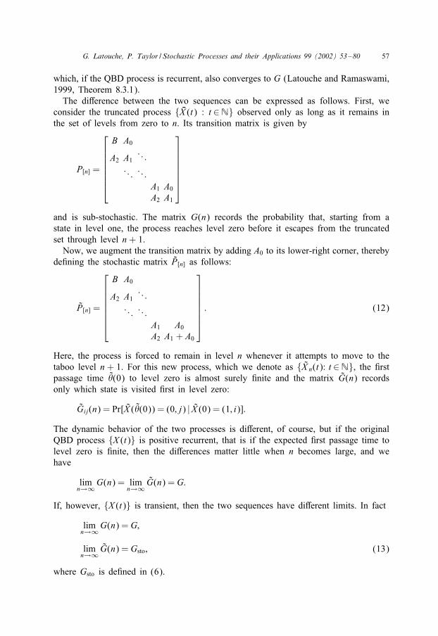
which, if the QBD process is recurrent, also converges to G (Latouche and Ramaswami,1999, Theorem 8:3:1).The di7erence between the two sequences can be expressed as follows. First, we

consider the truncated process { KX (t) : t ∈N} observed only as long as it remains inthe set of levels from zero to n. Its transition matrix is given by

P[n] =

B A0

A2 A1. . .

. . .. . .A1 A0A2 A1

and is sub-stochastic. The matrix G(n) records the probability that, starting from astate in level one, the process reaches level zero before it escapes from the truncatedset through level n+ 1.Now, we augment the transition matrix by adding A0 to its lower-right corner, thereby

de3ning the stochastic matrix P[n] as follows:

P[n] =

B A0

A2 A1. . .

. . .. . .A1 A0A2 A1 + A0

: (12)

Here, the process is forced to remain in level n whenever it attempts to move to thetaboo level n + 1. For this new process, which we denote as {X n(t): t ∈N}, the 3rstpassage time �(0) to level zero is almost surely 3nite and the matrix G(n) recordsonly which state is visited 3rst in level zero:

Gij(n) = Pr[X (�(0)) = (0; j) | X (0) = (1; i)]:

The dynamic behavior of the two processes is di7erent, of course, but if the originalQBD process {X (t)} is positive recurrent, that is if the expected 3rst passage time tolevel zero is 3nite, then the di7erences matter little when n becomes large, and wehave

limn→∞G(n) = lim

n→∞ G(n) = G:

If, however, {X (t)} is transient, then the two sequences have di7erent limits. In fact

limn→∞G(n) = G;

limn→∞ G(n) = Gsto; (13)

where Gsto is de3ned in (6).


The 3rst three limits are proved, for example, in (Latouche and Ramaswami, 1999,Theorems 8:1:1, 8:3:1). The fourth one is a direct consequence of Theorem 3 provedin this paper.As noted in Section 1, we address a more general modi3cation than the one consid-

ered in (12): we assume that the structure of the original QBD process is modi3ed atits level n according to (9). In the modi3ed process

Pr[X (1) = (n+ 1; j) |X (0) = (n; i)] = ( KA0)ij ;

Pr[X (1) = (n; j) |X (0) = (n; i)] = ( KA1)ij ;

Pr[X (1) = (n− 1; j) |X (0) = (n; i)] = ( KA2)ij ;

where KA0, KA1 and KA2 are nonnegative matrices, such that KA0+ KA1+ KA2 is stochastic. Wedenote the new process by {Yn(t): t ∈N}. The matrix K(n) of 3rst passage probabilitiesfrom level one to level zero in Yn(t) can be de3ned by

Kij(n) = Pr[ K�(0)¡∞ and Yn( K�(0)) = (0; j) |Yn(0) = (1; i)]:

The question which we wish to answer is the following: does the sequence {K(n):n¿ 1} converge as n tends to in3nity, and if so, what is its limit? In general, thisis a complicated question. Because we have imposed only mild restrictions on KA0,KA1 and KA2, we can change the reachability structure of the states in complicated ways.For example, take the QBD process with

A0 =

0 1 0 00 0 p 00 0 0 pp1 0 0 p2

; A1 = 0; A2 =

0 0 0 0q 0 0 00 q 0 00 0 q1 q2

(14)

and modify the transitions at level n so that

KA0 =

0 0 0 00 0 0 00 0 0 0p1 0 0 p2

; KA1 =

0 1 0 0p=2 0 p=2 00 p 0 00 0 0 0

; KA2 = A2: (15)

The transition graphs of the original and modi3ed processes are given in Fig. 1. It isclear that the original process satis3es Condition 1. However, in the modi3ed process,there is no escape from the set of states {(n − 2; 1), (n − 1; 2), (n − 1; 1), (n; 1),(n; 2), (n; 3)}. In order to derive our results, we must rule out cases like this, wherethe modi3cation creates a pocket of states in which {Yn(t): t ∈N} can get trapped.Condition 2 below serves this purpose.

Condition 2. The modi8ed matrix KPn is such that for every state (n; i) there is a pathto level zero.

In most cases, it is easy to verify by inspection of the modi3ed transition graph ifthis condition holds. A suNcient condition is that ( KA1)ij ¿ 0 for all i, j such that (A1+


Fig. 1. Part of the transition graph for two QBD processes. The one with blocks A0, A1 and A2 given in(16) is shown above, the one with the modi3ed matrices KA0, KA1 and KA2 given in (17) is shown below.

A0)ij ¿ 0 and ( KA2)ij ¿ 0 if (A2)ij ¿ 0; to show this, one follows the steps in the proofof (Latouche and Ramaswami, 1999, Theorem 8:3:1). If KA0, KA1 and KA2 do not satisfythis property and if the graph is complex, then one may apply standard reachabilityalgorithms to the 8nite transition graph obtained by replacing KA1 by KA1 + KA0G and KA0by 0 in (9).Condition 2, nevertheless, leaves us with a great deal of freedom to modify the

process. In our second example, there are phases i such that, starting from (n; i), themodi3ed process can reach only 3nitely many higher levels, while for other phases,the process may reach any level n′¿ n+1. In this example, the transition matrices are

A0 =

0 1 0 00 p=2 p=2 00 0 0 p0 0 0 0

; A1 = 0; A2 =

0 0 0 0q=2 q=2 0 00 q 0 00 0 1 0

: (16)

If we change the transition matrices at level n to

KA0 =

0 1 0 00 0 p 00 0 0 p0 0 0 0

; KA1 = A1; KA2 = A2; (17)

we 3nd that from (n; 1) all the levels remain reachable, but if the process starts in oneof the states (n; 2)− (n; 4) or in a lower level, then it cannot reach beyond level n+2.This is illustrated in Fig. 2.Although they complicate matters, we do not rule out such modi3cations of the

reachability structure of the QBD process.


Fig. 2. Part of the transition graph for two QBD processes. The one with blocks A0, A1 and A2 given in(16) is shown above, the one with the modi3ed matrices KA0, KA1 and KA2 given in (17) is shown below.

We shall say that a matrix K is properly sub-stochastic if it is sub-stochastic withspectral radius sp(K)¡ 1. This means that K is the transition matrix for a set of statesfrom which escape occurs in a 3nite time a.s. This holds if and only if the series∑

�¿0 K� converges and only if I −K is nonsingular by the Neumann Lemma (Ortega

and Rheinboldt, 1970, p. 45) in which case∑

�¿0 K� = (I − K)−1.

For similar reasons to those which justi3ed the fact that the matrices G(n) satisfythe recursion (10) and (11), the matrices K(n) satisfy the iterative equations

K(1) = KG; (18)

K(n+ 1) = [I − A1 − A0K(n)]−1A2; (19)

where

KG = [I − KU ]−1 KA2 (20)

and

KU = KA1 + KA0G: (21)

The inverse matrices in (19) and (20) exist for the following reason. The matrixA1 + A0K(n) records the 3rst return probabilities from the level 1 back to level 1,avoiding level 0, for the modi3ed process {Yn+1(t)}; similarly, KU records the 3rstreturn probabilities from the level n to the level n, avoiding level n − 1, for themodi3ed process {Yn(t)}. By Conditions 1 and 2, with probability one, it is not possiblerepeatedly to return to the same level without either visiting the level 0 or drifting toin3nity. Thus, A1 + A0K(n) and KU are both properly sub-stochastic.The following theorem provides the answer to our question about the convergence

of the sequence {K(n)}.


Theorem 3. Assume that Conditions 1 and 2 hold.If there is a number n∗¡∞ such that, whenever n¿ n∗, there is a path from level

zero to all levels in the Markov chain {Yn(t)}, thenlimn→∞K(n) = G;

the minimal nonnegative solution of (5).If, on the contrary, there exists no such n∗¡∞ then

limn→∞K(n) = Gsto = G + (I − G)1 · +:

Remark 4. Clearly; if KA0 = 0; KA1 = A1 + A0 and KA2 = A2; then there is no path fromlevel 0 to level n′ for any n′¿ n+ 1; so that

limn→∞ G(n) = lim

n→∞K(n) = Gsto;

which proves (13).

Before proving the theorem in Section 5, we need to establish several intermediateresults. First, we give an expression for K(n) in terms of 3rst passage probabilitiesbetween levels for the QBD process with transition matrix (1). For 16 s6 k, de3nethe matrices G(s; k) and H (s; k) by

Gij(s; k) = Pr[�(0)¡�(k + 1) and X (�(0)) = (0; j) |X (0) = (s; i)] (22)

and

Hij(s; k) = Pr[�(k + 1)¡�(0) and X (�(k + 1)) = (k + 1; j) |X (0) = (s; i)]: (23)

These matrices respectively record the 3rst passage probabilities from level s to level 0before level k+1, and from level s to level k+1 before level 0. Note that G(1; n)=G(n).

Theorem 5. Under Condition 2; the matrix K(n) of 8rst passage probabilities fromlevel one to level zero for the QBD process (9) is given by

K(n) = G(1; n− 1) + H (1; n− 1)[I − KGH (n− 1; n− 1)]−1 KGG(n− 1; n− 1):(24)

Proof. If we decompose the event [ K�(0)¡∞] into [ K�(0)¡ K�(n)] and [ K�(n)¡ K�(0)¡∞]; we readily 3nd that

K(n) = G(1; n− 1) + H (1; n− 1)D(n); (25)

where Dij(n) = Pr[ K�(0)¡∞ and Yn( K�(0)) = (0; j) |Yn(0) = (n; i)].Starting from level n, the process {Yn(t)} must pass through level n − 1 before

reaching level zero, and the matrix KG de3ned in (20) records the corresponding 3rstpassage probabilities, independently of n. Once in level n−1, the process behaves like


{X (t)} until it returns to level n. Thus, we obtain that

D(n) = KG[G(n− 1; n− 1) + H (n− 1; n− 1)D(n)]

=∑�¿0

[ KGH (n− 1; n− 1)]� KGG(n− 1; n− 1):

The theorem will have been proved once we show that the series converges.The matrix KGH (n− 1; n− 1) records the probability that, starting from level n, the

process eventually moves down to level n − 1 and later returns to level n withoutvisiting level zero. As a consequence of Condition 2, with probability one this cannotoccur inde3nitely: either the process ceases to return to level n − 1 altogether, or iteventually reaches level zero. Therefore, KGH (n − 1; n − 1) is properly sub-stochasticand the series converges.

3. Transition structure

It will be useful to consider the doubly in3nite QBD process {W (t)} with transitionmatrix (2). In addition to the matrix G, which records the 3rst passage probabilitiesfrom level n down to level n−1, we also de3ne the matrix H of 3rst passage probabil-ities from level n− 1 up to level n. This matrix has properties which are analogous tothose of G. For instance, H is the minimal solution of the equation H=A0+A1H+A2H 2.

De3ne != sp(G) and "= sp(H). With � as de3ned in (3), we know that• if �¡ 0, then G is stochastic with != 1 and H is sub-stochastic with "¡ 1;• if � = 0, then both G and H are stochastic and != "= 1;• if �¿ 0, then G is sub-stochastic with !¡ 1 and H is stochastic with "= 1.The stated properties of G are given in Latouche and Ramaswami (1999, Theorems7:1:1 and 7:2:3); they hold for H by symmetry.We also know by Latouche and Ramaswami (1999, Theorem 7:2:1) that if A is

irreducible (which, recall, is a consequence of Condition 1) then either G is irreducible,or it can be written, possibly after a permutation of its rows and columns, as

G =[G1 0G•1 G•

]; (26)

where G1 is irreducible and G• is lower triangular with its diagonal entries equal tozero.By the same argument, either H is irreducible, or it can be written as

H =[H1 0H•1 H•

]; (27)

where H1 is irreducible and H• is lower triangular with its diagonal entries equal tozero.We actually need a stronger property, which we prove in the next lemma; the method

of proof is similar to that of Theorem A:1 in Latouche and Taylor (2000).


Lemma 6. If Condition 1 holds; then either the matrix G is primitive or it has theform (26) where G1 is primitive. Similarly; either the matrix H is primitive or it hasthe form (27) where H1 is primitive.

Proof. We assume that G is irreducible; as the proof is easily adapted to the casewhere it has the structure (26). Also; we demonstrate the stated property for G only;the proof for H being similar.We proceed by contradiction. Assume that G is periodic, with period #. Then, there

exist phases i and j such that [Gk#]ij = 0 for all k. This implies that the process{W (t): t ∈N} with transition matrix (2) cannot reach state (1; j) from state (k#+1; i)without visiting some other state in level one 3rst. However, since G is irreducible,there exists some phase i∗ such that [Gk#−1]i∗j ¿ 0, so that there exists a path from(k#; i∗) to (1; j) which avoids level one in all its intermediate steps. It follows that, forany k¿ 1, it is impossible to visit (k#; i∗) from (k# + 1; i) without visiting level one3rst.By the spatial homogeneity of the doubly-in3nite process, we deduce that, for any

k¿ 1, it is impossible to visit (0; i∗) from (1; i) without visiting level −k# + 1 3rst.Therefore, it is impossible to visit (0; i∗) from (1; i) at all, which contradicts Condition1. We conclude that G is aperiodic. As an irreducible and aperiodic matrix is primitiveby Seneta (1981, Theorem 1:4), the lemma is proved.

De3ne the subset $∗ of phases as follows: if H is primitive, then $∗={1; 2; : : : ; m}.Otherwise, $∗ is the index set of H1. The following result, which is an immediateconsequence of Lemma 6, will be useful later.

Lemma 7. If Condition 1 holds; then there exists k∗ such that for all k¿ k∗; and16 i6m; (Hk)ij ¿ 0 if j∈$∗ and (Hk)ij = 0 if j ∈ $∗.

Proof. If $∗ = {1; : : : ; m}; then the property holds by de3nition of a primitive matrix(Seneta; 1981; p. 3). If $∗ is a proper subset of {1; : : : ; m}; then we have; after asuitable permutation of rows and columns;

H k =

[Hk

1 0

H (k)•1 Hk

•

]

for all k¿ 1; where

H (k)•1 = H (k−1)

•1 H1 + Hk−1• H•1: (28)

Since H• is lower triangular with diagonal entries zero; there exists some index k1such that Hk

• = 0 for all k¿ k1; which implies that (Hk)ij = 0 for k¿ k1 and j ∈ $∗.It follows that; for all k¿ k1 + 1;

H (k)•1 = H (k−1)

•1 H1 = H(k1)•1 H

k−k1−11 : (29)

By Condition 1; there is a path in {W (t)} from (0; i) to level k for all i and k. Thisimplies that for all i ∈ $∗; there is some j∈$∗ such that (H (k1)

•1 )ij ¿ 0. Because the


matrix H1 is primitive; there exists some index k2 such that Hk1 ¿ 0 for all k¿ k2; so

that; by (29); H (k)•1 ¿ 0 for k¿ k1 + k2 + 1. This proves the lemma.

By an argument identical to that which shows that G(1; n) → G as n→ ∞, one canshow that H (n− 1; n− 1) → H as n → ∞. Thus, in view of (24) it is clear that weneed to study the structure of the matrix KGH . This we now do.Consider the doubly in3nite QBD process {Wn(t)} with transition matrix

KTn =

. . .. . .

. . . A1 A0A2 A1 A0

KA2 KA1 KA0A2 A1 A0

. . .. . .

. . .

; (30)

where the modi3cation occurs at level n.The matrix KGH records the probabilities that, starting from a state in level n, this

process eventually moves down to level n−1 and, after that, eventually returns to leveln. In short, KGH is the matrix of eventual return probabilities to level n after a visit tolevel n− 1, starting from level n.

Lemma 8. Under Conditions 1 and 2; KGH has a unique essential class of indices;that is; either it is irreducible; or there can be a permutation of rows and columnssuch that

KGH =[C1 0C•1 C•

](31)

with C1 irreducible; but there is no permutation such that

KGH =

C1 0 00 C2 0C•1 C•2 C•

(32)

with C1 and C2 irreducible.

Proof. Assume to the contrary that KGH has the form (32); and denote by I1(n) andI2(n) the index sets of C1 and C2; respectively and by ‘1(n) and ‘2(n) the subsets ofstates (n; j) in level n with j∈ I1(n) and I2(n); respectively.Further, for �=1; 2, de3ne the subsets ‘�(n− 1) of level n− 1, and their associated

sets of phases I�(n− 1) by

I�(n− 1) = {j such that KGij ¿ 0 for some i in I�(n)};‘�(n− 1) = {(n− 1; j): j∈ I�(n− 1)}:


By the de3nition of KG, this means that ‘�(n−1) is the set of all the states which arereachable from above by the process {Wn(t)}, starting from some state in ‘�(n). Here‘reachable from above’ means that there is a path for which all intermediate states arein levels n to ∞.Step 1. For �= 1; 2, if i∈ I�(n− 1) and j ∈ I�(n), then Hij = 0. This follows since

there must be some i0 ∈ I�(n) for which KGi0i ¿ 0 and we have

0 = ( KGH)i0j¿ KGi0iHij:

We conclude that Hij = 0.Step 2. De3ne L�(n−1) as the set of all the states in levels zero to n−1 which are

reachable from at least one state in ‘�(n− 1), avoiding level n. Then, the intersectionof L1(n− 1) and L2(n− 1) is empty.To see this, assume that the intersection is not empty and take (k; j)∈L1(n − 1) ∩

L2(n−1). Observe that, by Condition 1, the process {W (t)} with transition matrix (2)is irreducible so that, for all k6 n and all j, there is a path from (k; j) to level n.Thus, there is an i0 such that there is a positive probability that (n; i0) is the 3rst statevisited in level n, starting from (k; j). It follows that (Hn−k)j; i0 ¿ 0.

By de3nition of L1(n − 1), there is a state (n − 1; j0) in ‘1(n − 1) such that thereis a path from (n− 1; j0) to (k; j) avoiding level n. Therefore, we have that Hj0i0 ¿ 0and so i0 ∈ I1(n) by Step 1. By the same argument, i0 ∈ I2(n), which is a contradictionsince I1(n) ∩ I2(n) is empty by de3nition. Therefore L1(n− 1) ∩ L2(n− 1) is empty.

Step 3. As the doubly in3nite QBD process {W (t)} is irreducible, for all j and j′,there is a path of 3nite length from (0; j) to (0; j′). For any such path P, let )(P)be the maximal level reached on that path, and let *(j; j′)=min{)(P)} where theminimum is taken over all paths from (0; j) to (0; j′). Finally, de3ne *∗

=max{*(j; j′): 16 j; j′6m}. Then, for n¿*∗, Step 2 implies that either L1(n− 1)contains no states at level zero, or L2(n− 1) contains no states at level zero, or both.If this were not the case, then we would 3nd two states (0; j) in L1(n−1) and (0; j′)

in L2(n− 1) such that there is a path from (0; j) to (0; j′) wholly contained in levelszero to n−1, so that (0; j′) would also belong to L1(n−1), in contradiction with Step 2.

Step 4. Assume, without loss of generality, that L1(n−1) contains no states at levelzero. Then there is no path from ‘1(n) to level zero.Starting from a state in ‘1(n), the QBD process {Yn(t)} with the modi3ed transition

matrix (9) can eventually move down to a state in ‘1(n− 1) from which it will not beable to reach level zero before returning to level n. Upon return to level n, the processis again in ‘1(n) by Step 1, so that it will never reach level zero.This contradicts Condition 2 and so we conclude that KGH cannot have the

structure (32).

4. First passage probabilities

We determine in this section the asymptotic properties of the various 3rst passageprobability matrices which appear in (24). For this, we need the expressions given in


Theorem 10, which are similar to those in Hajek (1982). Before we prove this theorem,we need the following lemma.

Lemma 9. If � =0; then the matrices HkGk and GkHk are properly sub-stochastic;that is; sp(HkGk)¡ 1; sp(GkHk)¡ 1 and the matrices I − HkGk and I − GkHk arenonsingular.

Proof. The (i; j)th entry of the matrix GkHk is the probability that the process {W (t)}starts from (k; i); reaches level 0 and then returns to level k in state (k; j) after a 3niteamount of time. Thus; [

∑�¿0 (G

kHk)�]ij is the expected number of visits to (k; j)immediately following a visit to level zero; starting from (k; i).

This number of visits is smaller than the expected total number of visits to (k; j).As � =0, the process {W (t)} is transient, the expected total number of visits to anystate is 3nite and the series converges. This, in turn, implies that

∑�¿0

(HkGk)� = I + Hk

[∑�¿0

(GkHk)�]Gk

converges as well. This implies that sp(HkGk) and sp(GkHk) are strictly ¡ 1, and theother stated properties follow.

If �=0, the matrices G and H are stochastic and so are HkGk and GkHk for all k.

Theorem 10. If � =0; then the matrices G(s; k) and H (s; k) de8ned in (22) and (23)are given by

G(s; k) = (I − Hk+1−sGk+1−s)Gs(I − Hk+1Gk+1)−1; (33)

H (s; k) = (I − GsHs)Hk+1−s(I − Gk+1Hk+1)−1 (34)

for 16 s6 k.

Proof. We 3rst show that the matrices are solutions of the system

[G(s; k) H (s; k)]

[I Hk+1

Gk+1 I

]= [Gs Hk+1−s]: (35)

The matrix Gs records the 3rst passage probabilities of {W (t)} from level s to levelzero. If we decompose those probabilities according to whether �(0)¡�(k+1) or �(0)¿�(k + 1), we readily 3nd that

Gs = G(s; k) + H (s; k)Gk+1:

By symmetry,

Hk+1−s = H (s; k) + G(s; k)Hk+1:

This proves (35).


If � =0, then, by Lemma 9, I −HnGn and I −GnHn are nonsingular for n¿ 1 andone proves by direct veri3cation that[

I Hn

Gn I

]−1

=[

I −Hn

−Gn I

] [(I − HnGn)−1 0

0 (I − GnHn)−1

];

which, together with (35), proves (33) and (34).

Assume henceforth that � =0. It follows in particular from Theorem 10 that

G(1; n− 1) = (I − Hn−1Gn−1)G(I − HnGn)−1; (36)

H (1; n− 1) = (I − GH)Hn−1(I − GnHn)−1; (37)

G(n− 1; n− 1) = (I − HG)Gn−1(I − HnGn)−1 (38)

and

H (n− 1; n− 1) = (I − Gn−1Hn−1)H (I − GnHn)−1: (39)

We now investigate the asymptotic behavior of these matrices, as n → ∞. This iswhere we shall make use of Lemma 6.

Lemma 11. If Condition 1 holds; then

Gn = !nC · ++ o(!n) (40)

asymptotically as n→ ∞; where + and C are the unique left- and right-eigenvectorsof G associated with !; normalized such that +1= 1; +C= 1.If G is primitive, then + and C are strictly positive. If G has the form (26), then

+= [+1 0];

where +1 is the strictly positive eigenvector of G1 with the eigenvalue !, and

C=[C1C2

];

where C1 is the strictly positive right-eigenvector of G1 with eigenvalue !, andC2 = (!I − G•)−1G•1C1.

If != 1; o(1) represents a quantity which tends to zero as n→ ∞.

Proof. If G is primitive; this is a consequence of Seneta (1981; Theorem 1:1; p. 3 andTheorem 1:2; p. 9). If G has the form (26); then the nonzero eigenvalues of G arethose of G1. As G1 is primitive; its maximal eigenvalue ! has algebraic multiplicityone and the other eigenvalues have modulus which is strictly less than !; so that (40)still holds.The proof that C and + are as given, when G has the form (26), is by direct

veri3cation.

A similar property holds for H . We state it without proof.


Lemma 12. If Condition 1 holds; then

Hn = "nw · h+ o("n) (41)

asymptotically as n→ ∞; where h and w are the unique left- and right-eigenvectorsof H associated with "; normalized such that h1= 1; hw= 1.If H is primitive, then h and w are strictly positive. If H has the form (27), then

h= [h1 0];

where h1 is the strictly positive eigenvector of H1 with the eigenvalue ", and

w=[w1

w2

];

where w1 is the strictly positive right-eigenvector of H1 with eigenvalue ", andw2 = ("I − H•)−1H•1w1.

In view of these two lemmas, when � =0 we can directly write

GnHn = c1-nC · h+ o(-n) as n→ ∞; (42)

where - = !"¡ 1 and c1 = +w, andHnGn = c2-nw · ++ o(-n) as n→ ∞; (43)

where c2 = hC. We also have, as n→ ∞,

(I − GnHn)−1 = (I − c1-nC · h)−1 + o(-n)= I + c1-n(1 + c1-nhC)−1C · h+ o(-n)

by the Sherman–Morrison formula (Golub and Van Loan, 1989, p. 51), so that

(I − GnHn)−1 = I + c1-nC · h+ o(-n) as n→ ∞: (44)

Similarly,

(I − HnGn)−1 = I + c2-nw · ++ o(-n) (45)

as n→ ∞.

5. Convergence of the matrix sequences

We are now ready to analyze the asymptotic behavior of the sequence {K(n)}, usingthe expression given in Theorem 5. We 3rst rapidly deal with the case where the QBDprocess {X (t)} with transition matrix (1) is recurrent.

Theorem 13. If �6 0 and if the matrices KA0; KA1 and KA2 are such that Condition 2holds; then limn→∞ K(n) = G.

Proof. We know that limn→∞G(1; n) = G always; and that G1 = 1 if �6 0. Wealso have that K(n)16 1 for all n. Finally; K(n)¿G(1; n − 1) by (25). Therefore;limn→∞ K(n)1= 1 and limn→∞H (1; n− 1)D(n)1= 0.


As H (1; n − 1)D(n)¿ 0, this implies that limn→∞H (1; n − 1)D(n) = 0 so thatlimn→∞ K(n) = limn→∞G(1; n− 1).

We can now concentrate on the case where the QBD process {X (t)} is transient,that is where �¿ 0. Then !¡ 1 and "= 1, which implies that -= !; H is stochastic,w= 1 and c1 = 1. It immediately follows from (36)–(39) and (40)–(45) that

G(1; n− 1) = G + O(!n); (46)

H (1; n− 1) = (I − G)1 · h+ o(1); (47)

G(n− 1; n− 1) = !n−1(I − !H)C · ++ o(!n) (48)

and

H (n− 1; n− 1) = H − !n−1(I − !H)C · h+ o(!n): (49)

There are three types of modi3cation which can be brought to the dynamics of theprocess by the change of transition probabilities at level n. These are characterized asfollows.

(1) sp( KGH)¡ 1. Here, all levels are reachable from any state in levels zero to n and,like {X (t)}, the QBD process {Yn(t)} drifts towards in3nity.

(2) sp( KGH)=1 because KGH is stochastic, which can occur only if KG itself is stochastic.As we shall see, this means that the modi3ed QBD process {Yn(t)} has no pathto in3nity. Instead, there exists some n such that, starting from any state in leveln, the process cannot move higher than level n+ n.

(3) sp( KGH) = 1 although KGH is not stochastic. This implies that, starting from somestates (n; i), the process can reach all levels n′¿ n, and starting from other states(n; i), there exists some n such that the process cannot move higher than leveln + n. We shall show that, for n large enough, the process cannot move higherthan level n+ n if it starts in level one.

In case 1, the series∑

�¿0 ( KGH)� converges, it diverges in the other cases.

In cases 2 and 3, at least for n large enough, the state space of the process {Yn(t)}is partitioned into one 3nite irreducible class which contains level one, and one ormore transient classes. In these cases, the matrix K(n) is stochastic and the sequence{K(n)} converges to Gsto. In case 1, the process {Yn(t)} remains transient, K(n) issub-stochastic but not stochastic for all n and the sequence {K(n)} converges to G.These claims are now proved.

Lemma 14. Assume that Condition 1 holds. If �¿ 0 and if sp( KGH)¡ 1; then thereexists n∗ such that for all n¿n∗ and for all phases i; there is a positive probabilitythat the process {Yn(t)} does not reach level zero if it starts in state (n; i).Moreover, for n¿n∗, K(n)16 1 with at least one strict inequality.

Proof. If sp( KGH)¡ 1; then the series∑

�¿0 ( KGH)� converges and �=∑

�¿0 ( KGH)�1is 3nite. The vector � has the following interpretation: /i is the expected number of


times that the doubly in3nite process {Wn(t)} with transition matrix (30) returns tolevel n after a visit to level n− 1; starting from (n; i).As H is stochastic, {Wn(t)} almost surely returns to level n after each visit to level

n − 1. Thus, /i ¡∞ implies that there is a positive probability that, after a last visitto level n− 1, the process {Wn(t)} reaches some state (n; j0) and does not visit leveln− 1 thereafter. Let (n−D) be the lowest level reached by the process along the pathfrom (n; i) to (n; j0). The random variable D can be thought of as the “depth” of apath from (n; i) to (n; j0). It is 3nite almost surely, and so there must exist an n∗ suchthat D¡n∗ with positive probability.If we choose n such that n¿n∗ then there is a positive probability that {Wn(t)}

never reaches level zero starting from (n; i). For this value of n, the same event in{Yn(t)} also has positive probability, and so there is a positive probability that {Yn(t)}never reaches level zero starting from (n; i). This proves the 3rst part of the lemma.There must be at least one phase i such that, starting from (1; i), it is possible for

{Yn(t)} to reach level n before level zero. After reaching level n, the process has apositive probability of not reaching level zero. Thus, the probability 1 − (K(n)1)i ofnever reaching level zero when starting from (1; i) is strictly positive.

In view of the arguments above, it is clear that when sp( KGH)¡ 1, it is possiblefor {Yn(t)} to reach level n from any state in the lower levels and not return to theset of levels zero to n thereafter. Thus, either there is positive probability that {Yn(t)}drifts to in3nity, or there is a positive probability that it remains within a 3nite set oflevels above level n. The second circumstance is in contradiction with Condition 2 thatthere must be a path from any state to level zero and so the 3rst circumstance mustbe the case. The process {Yn(t)} is thus transient with drift to in3nity. This is case 1discussed above.

Lemma 15. Assume that Condition 1 holds and that �¿ 0; let ‘s(n) be the set ofstates (n; i) for which [ KGH1]i = 1. There exists some 8nite n such that; starting in‘s(n); the process {Yn(t)} cannot reach level n+ n before going down to level n− 1.

Proof. For any k and j; the probability of not reaching level n−1 if the process startsin (n+ k; j) is greater than the probability of not reaching level n starting in (n+ k; j)which is equal to 1 − (Gk1)j. By Lemma 11; there exists some n such that Gk1¡ 1for all k¿ n. Therefore; for k¿ n; there is a positive probability of not reaching leveln − 1 starting in any state of the form (n + k; j). It follows that; if it is possible toreach level n+ n before level n− 1 starting from (n; i); then there must be a positiveprobability of never reaching level n − 1 and [ KGH1]i ¡ 1. The result is stated aboveas the contrapositive of this.

The proof of the corollary below is immediate.

Corollary 16. Assume that Condition 1 holds. If �¿ 0 and sp( KGH) = 1; then thereexists n¡∞ such that the process cannot reach level n+ n; if it starts in levels zeroto n.


As a consequence, we see that, if KG1 = 1, the states in level zero and level onebelong to a 3nite irreducible class, so that they are positive recurrent and K(n) isstochastic. This is case 2 described above.In order to analyze the more complex case 3, de3ne two subsets of states ‘e(n)

and ‘p(n) as follows. The subset ‘e(n) contains those states in level n for which thereexists a path in {Wn(t)} to level n′ for all n′¿ n. The subset ‘p(n) contains the otherstates in level n. In case 3, both subsets are nonempty as we now show.The 3rst hypothesis that de3nes case 3 is that there exists some i such that ( KGH1)i=

( KG1)i ¡ 1. This means that if the process {Wn(t)} starts in (n; i), there is a positiveprobability that it never visits level n − 1. Thus, as in case 1 above, this means thatthere must be a path in {Wn(t)} from (n; i) to all levels n′¿ n. This shows that thesubset ‘e(n) is nonempty.The second assumption relating to case 3 is that

∑�¿0 ( KGH)� does not converge

for some indices. This implies that KGH is reducible and so must have the form (31)with C1 a stochastic matrix. Let I1(n) denote the set of phases corresponding to thesub-matrix C1 and ‘1(n) the set of states (n; i) with i∈ I1(n). By Lemma 15, startingfrom a state in ‘1(n), there exists some n such that it is impossible for the processto move beyond level n+ n before going down to level n− 1. By the structure (31),the process is forced to return to ‘1(n) after going down to level n− 1. Therefore, theprocess cannot reach any level n′ with n′¿n+ n. Thus, the set ‘p(n) contains at leastthe phases in ‘1(n).

Lemma 17. Assume that Conditions 1 and 2 hold. Furthermore; assume that �¿ 0;that ( KG1)i ¡ 1 for some i; and that sp( KGH) = 1. There is a number n∗ such that;for n¿ n∗; there exists no path from level one to all levels n′¿ n. Furthermore; forn¿ n∗; the number of states in levels zero to n from which there exists a path in{Yn(t)} to all levels n′¿ n is independent of n.

Proof. Consider k∗ and $∗ as de3ned in Lemma 7. We shall show that(a) if {Yn(t)} starts in a state of the form (n− k; i) for n¿k¿ k∗; then the 3rst state

which it visits at level n must be of the form (n; j) with j∈$∗; and(b) there is a k such that; for all n¿ k; (n; j) with j∈$∗ is a state in ‘p(n) and thus

{Yn(t)} cannot escape to in3nity if its starts in (n; j).The consequences of (a) and (b) are that; for k¿ k∗ and n¿n∗ ≡ max(k; k); theprocess {Yn(t)} cannot escape to in3nity if it starts in a state of the form (n− k; i) andthe 3rst assertion of the lemma follows. Furthermore; for n¿ n∗; the set E(n) of allthe states in levels zero to n from which there exists a path to all levels is containedentirely within the levels from n − n∗ to n. For n¿ n∗; the transition structures ofthe processes {Yn(t)} on the levels n− n∗ to n are identical; which proves the secondstatement.To prove (a) above, de3ne Vk to be the 3rst passage probability matrix of {Yn(t)}

from level n − k − 1 back to level n − k − 1 avoiding level n. Conditioning on thelast visit to level n− k, we readily obtain that the 3rst passage probabilities from leveln− k − 1 to level n are given by

Wk = (I − Vk)−1A0H (1; k): (50)


A little reUection shows that H (1; k)6Hk , so that for every k¿ k∗ and j ∈ $∗, thejth column of H (1; k) is 0 and therefore the jth column of Wk is 0. This proves thatfor every starting state in level n − k∗ or below, the 3rst state in level n visited by{Yn(t)} must be of the form (n; j) with j in $∗. This constitutes the 3rst step of theproof.In the proof of (b), we 3rst show that there exists some k such that for every i in

{1; : : : ; m}, every j in $∗, every k¿ k and every n¿k, there exists a path in {Yn(t)}from (n−k; i) to (n; j) which avoids level n+1. Indeed, it follows from (47) and (50)that

Wk = (I − Vk)−1A0(I − G)1 · h+ o(1)

asymptotically as k tends to in3nity. Since Wk is a stochastic matrix for all k, thecolumn vector (I −Vk)−1A0(I −G)1 is strictly positive for k large enough. Moreover,it follows from Lemma 7 that hj ¿ 0 for all j in $∗. Thus, there exists k such that,for all k¿ k, i in {1; : : : ; m} and j in $∗, (Wk)ij ¿ 0.Now we show that, for n¿ k, every state of the form (n; j) with j∈$∗ is in ‘p(n).

Consider a starting state s in ‘p(n). By Condition 2, there is a path in {Yn(t)} from sto level zero. If we take n such that n¿ k, this implies that there is a path in {Yn(t)}from s to some state (n− k ; i). By the argument above, this in turn implies that, for allj in $∗, there is a path from s to (n; j). If any of these states (n; j) were in ‘e(n) thenit would be possible to escape to in3nity starting in s, which contradicts the de3nitionof ‘p(n). Thus all states of the form (n; j) where j∈$∗ must be in ‘p(n).This completes the proof of the lemma.

Corollary 5:3 and Lemmas 5:4 and 5:5 establish that, when �¿ 0, the e7ect of themodi3cations in the transition probabilities from level n is summarized in the matrixKGH . Speci3cally, under Conditions 1 and 2, one has that sp( KGH)¡ 1 if and only ifthere is a path from level one to level n′ for all n′. This is a property which can beveri3ed by inspection of the transition graph; in particular, it is satis3ed if KA2 = A2,KA1 = A1 + pA0, and KA0 = (1− p)A0 with 0¡p¡ 1.In order to simplify the notation in the proof of Theorem 3 below, we de3ne the

matrices

C(n) = KGH (n− 1; n− 1)

and

C = limn→∞C(n) =

KGH:

Proof of Theorem 3. We need to consider only QBD processes for which �¿ 0 since;for �6 0; convergence has been proved in Theorem 13.It is simplest to deal with case 1, where sp(C)¡ 1. Here, we show that

limn→∞ K(n) = G.


As H (n− 1; n− 1)6H for all n, we have

[I − C(n)]−1 =∑�¿0

C(n)� =∑�¿0

[ KGH (n− 1; n− 1)]�6∑�¿0

C�

so that [I−C(n)]−1 is uniformly bounded. One uses (24), (46)–(49) and easily obtainsthat K(n) = G + O(!n), from which the claim immediately results.In the other cases, sp(C)=1 and we show that limn→∞ K(n)=Gsto. Since I −C(n)

becomes singular as n→ ∞ the key feature is the analysis of the factor [I − C(n)]−1

in (24).Eq. (49) yields

C(n) = C − !n−1y · h+ o(!n);where

y= KG(I − !H)C:From Lemma 8, if sp(C)=1, the Perron–Frobenius eigenvalue of C is equal to one andit is simple. Denote its left and right eigenvectors as l and r, with l1= lr=1, and by4(n), l(n) and r(n) the maximal eigenvalue of C(n) and its eigenvectors, normalizedso that l(n)1= l(n)r(n) = 1.By Kato (1966, Theorem 5:4, p. 111), there exists 4∗ such that

4(n) = 1 + !n−14∗ + o(!n)

and l∗ and r∗ such that

l(n) = l + !n−1l∗ + o(!n)

and

r(n) = r + !n−1r∗ + o(!n):

Equating the coeNcients of !n−1 on both sides of the equations l(n)r(n) = 1 and4(n) = l(n)C(n)r(n), we obtain that

4∗ =−(ly)(hr): (51)

Let C(n) = C(n) − 4(n)r(n) · l(n), which has the e7ect of replacing the maximaleigenvalue of C(n) by zero without changing any other of its eigencharacteristics. Itfollows that

[I − C(n)]−1 = [I − C(n)]−1 + 4(n)(1− 4(n))−1r(n) · l(n)by the Sherman–Morrison formula, or

[I − C(n)]−1 = [I − C(n)]−1 − 1!n−14∗

r · l + O(1);

where O(1) is a quantity that remains bounded as n tends to in3nity.It follows from Kato (1966, p. 107) that the eigenvalues of C(n) apart from 4(n) are

bounded away from one, and so the matrix [I − C(n)]−1 remains bounded as n→ ∞and

[I − C(n)]−1 =− 1!n−14∗

r · l + O(1): (52)


Combining this equation with (24), (46)–(48), (51), we easily verify that K(n)=G+(I − G)1 · ++ o(1) which proves the result in this case.

Another formulation of Theorem 3, one which emphasizes the algebraic aspects, isas follows.Alternate formulation of Theorem 3. Under Conditions 1 and 2,• if �6 0, then limn→∞ K(n) = G = Gsto;• if �¿ 0 and sp( KGH) = 1, then limn→∞ K(n) = Gsto =G;• if �¿ 0 and sp( KGH)¡ 1, then limn→∞ K(n) = G =Gsto.With respect to this formulation, one may see Condition 2 as our way of guaranteeingthat the basic matrix KGH has (at most) a single eigenvalue 1.

6. Numerical stability

We return in this section to the starting point of our investigation, the recurrence(7). The initial matrix Z(0) is sub-stochastic, but otherwise arbitrary. Take KA2 = Z(0),KA1 = 0, KA0 = 1=m(1 − Z(0)1) · e, where e is a row vector of ones, and assume thatCondition 2 holds. Then Z(n)6K(n) for all n.If Z(0) is stochastic, then KA0 = 0, Z(n) =K(n) for all n and limn→∞ Z(n) =Gsto by

the second statement in Theorem 3. Alternatively, if Z(0) is strictly sub-stochastic, 2

that is, if Z(0)1¡ 1, then limn→∞ Z(n) = G, no matter how close Z(0) might beto Gsto.The indication seems to be that for a transient QBD process, G is a stable equilibrium

point for the recursion (7) while Gsto is not.Our purpose in this section is to prove this claim in a precise manner. In fact we

prove something more: we show that whenever the QBD process is not null-recurrent,there are two nonnegative 3xed points of (7), G and a second, which we denote byGmax, which is such that G6Gmax, G =Gmax. For transient processes, G6Gsto=Gmax

and for positive recurrent processes, G = Gsto6Gmax. Furthermore, we show that Gis a stable 3xed point of (7), whether G = Gsto or not, and Gmax is an unstable 3xedpoint of (7).Under Condition 1, the matrix polynomial A(z)=A0 + zA1 + z2A2 is nonnegative and

irreducible for z¿ 0. Its Perron–Frobenius eigenvalue 6(z) is positive, and its Perron–Frobenius right-eigenvector r(z) may be chosen to be strictly positive. By Neuts (1981,Lemma 1:3:4, Theorem 1:3:2) and Gail et al. (1998, Proposition 8), the equation 6(z)=zhas two solutions z=1 and z= 7 in (0;∞), with 7¡ 1 if the QBD process is positiverecurrent, and 7¿ 1 if it is transient (z=1 is the unique root of 6(z)= z if the processis null recurrent). Furthermore, the spectral radius of G is !=min(1; 1=7).The second solution of (5) is

Gmax = G + (4maxI − G)rmax +; (53)

2 If the matrix Z(0) is sub-stochastic but not strictly sub-stochastic, the discussion becomes more involved.


where + is the left Perron–Frobenius eigenvector of G, 4max = max(1; 1=7) and rmax =r(1=4max), normalized so that +1=+rmax =1. It is a simple matter to verify that, if theQBD process is transient, then Gmax = Gsto de3ned by (6).Represent by 〈0; Gmax〉 the set of matrices X such that 06X 6Gmax and de3ne the

operator M on 〈0; Gmax〉 such that MX = A1 + A0X .

Lemma 18. The spectral radius of the matrix Umax =MGmax is strictly less than one.

Proof. As Gmaxrmax = 4maxrmax; we have

Umaxrmax = (A1 + 4maxA0)rmax

= 4max(4−1maxA1 + A0)rmax

= 4max(4−1maxI − 4−2

maxA2)rmax

6 rmax

by de3nition of rmax. Thus; since rmax¿ 0; sp(Umax)6 1.Assume that sp(Umax) = 1. Then, there exists a vector u¿ 0 such that uUmax = u.

De3ne the sets S1 and S2 of indices i such that ui ¿ 0 and ui = 0, respectively. Fromu(A1 + A0Gmax) = u, A1¿ 0, A0Gmax¿ 0 and Gmax¿G, we conclude that

i∈ S1 ⇒ (A1)ij = (A0G)ij = 0; for all j∈ S2: (54)

We also have that

uGmax = uUmaxGmax

= u(A1Gmax + A0G2max)

= u(Gmax − A2)since Gmax is a solution of (5), so that uA2 = 0 and we conclude that

i∈ S1 ⇒ (A2)ij = 0; for all j: (55)

This leads us to the conclusion that the QBD process is not irreducible. Indeed, letthe process start at time 0 in state (1; i) with i∈ S1. By (55), the process cannot godirectly down to the level zero. By (54), the next state visited at level one is in{(1; j): j∈ S1} again. Thus, the process is not able to go to level zero at all, whichcontradicts Condition 1.

As a consequence of Lemma 18, for any V ∈ 〈0; Umax〉,∑

k¿0 Vk converges to the

nonnegative matrix [I − V ]−1 and so we can write Gmax = (I − Umax)−1A2. Similarlywe can write G = (I − U )−1A2, with U = A1 + A0G.We are also interested in the spectral properties of the matrix R discussed by

Neuts (1981). It follows from Eq. (8:2) of Latouche and Ramaswami (1999) thatR=A0(I −U )−1 and from Theorem 1:3:2 of Neuts (1981) that sp(R)=min(1; 7). Fur-thermore, it is easy to verify that Rmax=A0(I−Umax)−1 is a nonnegative solution of theequation R=A0+RA1+R2A2 and that sp(Rmax) is either equal to 1 or to 7. By Gail et al.


Table 1Spectral radii of the matrices G, Gmax, R and Rmax

Positive recurrent QBD Transient QBD

G = (I − U )−1A2 sp(G) = 1 sp(G) = 1=7¡ 1Gmax = (I − Umax)−1A2 sp(Gmax) = 1=7¿ 1 sp(Gmax) = 1R = A0(I − U )−1 sp(R) = 7¡ 1 sp(R) = 1Rmax = A0(I − Umax)−1 sp(Rmax) = 1 sp(Rmax) = 7¿ 1

(1994, Propositions 17 and 18), sp(Rmax) =sp(R), from which we conclude thatsp(Rmax) = max(1; 7).Thus we see that the matrices G, Gmax, R and Rmax take di7erent values for their

spectral radii, depending on whether the QBD process is transient or positive recurrent.The precise situation is summarized in Table 1.The recursion (7) may be written as Z(n+ 1) =GZ(n), where G is well de3ned in

〈0; Gmax〉. Its characteristics near the two 3xed points G and Gmax are given below.

Theorem 19. The operator G is Frechet-di=erentiable and; for every X in 〈0; Gmax〉;G′(X )H = (I −MX )−1A0H (I −MX )−1A2: (56)

If the QBD process is positive recurrent or transient; then the spectral radius ofG′(G) is strictly less than one; and the spectral radius of G′(Gmax) is strictly greaterthan one.

Proof. The 3rst statement is proved by repeating the argument of Latouche (1994;Lemmas 4:1 and 4:2). To prove the second; de3ne the column vector h = vec(H) asthe direct sum of the columns of H . Then (56) may be written as

G′(X )h= [(I − V )−1A2]T ⊗ [(I − V )−1A0]h;

where V =MX = A1 + A0X and ⊗ denotes the Kronecker product. We have

sp(G′(X )) = sp((I − V )−1A2)sp((I − V )−1A0)= sp((I − V )−1A2)sp(A0(I − V )−1):

Thus; we see from Table 1 that

sp(G′(G)) = sp(G)sp(R)¡ 1 (57)

and that

sp(G′(Gmax)) = sp(Gmax)sp(Rmax)¿ 1; (58)

which concludes the proof.

The consequence of this theorem is that G is a stable equilibrium point for (7) whileGmax is not: if we start the recursion from Z(0)=G+H for some small perturbation Hand iteratively compute {Z(n)} according to (7), then the di7erence from G will be-come smaller because sp(G′(G))¡ 1. On the contrary, if we start from Z(0)=Gmax+H ,the di7erence from Gmax might become bigger for some H because sp(G′(Gmax))¿ 1.


To illustrate this phenomenon, we took

A0 =

[0:4 0:2

0:2 0:2;

]; A1 = 0; A2 =

[0:3 0:1

0:5 0:1

];

which de3nes a transient QBD process. Computing G with the logarithmic reductionalgorithm in Latouche and Ramaswami (1993) we obtained after seven iterations anapproximation G such that

G − (A2 + A1G + A0G2) = 10−15

[0:111 0

0 0

]:

Next, we computed Gmax from (6) and obtained an approximation Gmax such that

Gmax − (A2 + A1Gmax + A0G2max) = 10−15

[0 0:0278

−0:111 −0:0278

]:

These approximations may be considered exact within machine precision. We 3nallycomputed four sequences from (7), starting with

Z1(0) = Gmax + 10−15I;

Z2(0) = Gmax − 10−15I;

Z3(0) = Gmax + 10−15

[1 −1

−1 1

]

and

Z4(0) =

[ 13

23

23

13

]:

The matrices Z1(0), Z2(0) and Z3(0) are very close to Gmax, Z4(0) is an arbitrarystochastic matrix. The results for the sequences 1, 2 and 4 are displayed in Table 2;we have not displayed the results for the third sequence because it converges after 7iterations to the matrix

Z4(7) = Gmax − 10−15

[0:67 0:19

0:33 0:11

];

which is very close to Gmax.The other three sequences eventually converge to G. The 3rst two columns in Table

2 are very similar: after 10 iterations, the distance to Gmax has already increased bya factor of 10 and, after 200 iterations, the distances to G and Gmax are of the sameorder of magnitude. The fourth sequence initially rapidly converges to Gmax, at theapproximate rate of one signi3cant digit per iteration, and Z4(10) is within 10−13 ofGmax. The precision improves for a few more iterations and then begins to deterioratein the same fashion as for the 3rst sequence.The second sequence constantly remains below Gmax (note that Z2(n)− Gmax is al-

ways negative), while the other two sequences are bigger than Gmax for a while. As


Table 2Behavior of three sequences. The 3rst two start from Z(0) =Gmax +H for a very small perturbation H , thelast one starts from an arbitrary stochastic matrix

Sequence 1 Sequence 2 Sequence 4

Z(10)− Gmax

10−14

[0:58 0:17

0:37 0:11

]10−14

[−0:60 −0:17

−0:38 −0:11

]10−13

[−0:58 0:60

−0:38 0:39

]

Z(20)− Gmax

10−13

[0:32 0:09

0:20 0:06

]10−13

[−0:33 −0:10

−0:22 −0:06

]10−14

[0:68 0:19

0:46 0:13

]

Z(40)− Gmax

10−12

[0:96 0:28

0:62 0:18

]10−11

[−0:10 −0:03

−0:07 −0:02

]10−12

[0:21 0:06

0:13 0:04

]

Z(100)− Gmax

10−7

[0:27 0:08

0:17 0:05

]10−7

[−0:28 −0:08

−0:18 −0:05

]10−8

[0:58 0:17

0:37 0:11

]

Z(200)− Gmax[−0:16 −0:05

−0:11 −0:03

] [−0:11 −0:03

−0:07 −0:02

] [−1:2 −0:35

−0:78 −0:23

]

Z(200)− G[−0:03 −0:01

−0:02 −0:01

] [0:02 0:01

0:01 0:00

] [−1:1 −0:31

−0:69 −0:20

]

Z(400)− G

10−15

[−0:89 −0:22

−0:67 −0:19

]10−15

[0:11 0:03

0 −0:03

]10−15

[−0:89 −0:22

−0:67 −0:19

]

a matter of fact, a closer examination of the 3rst and fourth sequence shows that,once Z(n) begins to diverge from Gmax, the sequence increases until sp(MZ(n)) be-comes ¿1, at which time Z(n + 1) ceases to be nonnegative. Then some of thematrices in the sequence have negative entries, until the sequence returns to the set of


sub-stochastic matrices and 3nally converges to G. For the fourth sequence, the rupturetakes place between the 198th and the 199th iterations: sp(MZ4(198)) = 0:8836 whilesp(MZ4(199)) = 2:0365 and

Z4(200) =

[−0:4371 −0:1139

0:0310 −0:0359

]:

The next iteration already is sub-stochastic.

7. Conclusions

Theorem 3 applies to continuous-time as well as to discrete-time QBD processes.Also, it applies to more general modi3cations of the transition structure. To see this,

de3ne the process {Yn;m(t): t ∈N} involving modi3cations of the transition probabilitiesin levels n to n+ m to be

Pr[X (1) = (n+ k + 1; j) |X (0) = (n+ k; i)] = (A(k)0 )ij ;

Pr[X (1) = (n+ k; j) |X (0) = (n+ k; i)] = (A(k)1 )ij ;

Pr[X (1) = (n+ k − 1; j) |X (0) = (n+ k; i)] = (A(k)2 )ij

for 06 k6m, and denote by Km(n) the matrix of 3rst passage probabilities from levelone to level zero for this new process.If we assume that, for every state (n + k; i) with 06 k6m, there exists a path to

level n− 1 or to level n+ m+ 1 or both, then Theorem 3 applies.To establish this, de3ne two matrices of 3rst passage probabilities outside of levels

n to n+ m:

(GA)ij = Pr[�(n− 1)¡�(n+ m+ 1);

and X (�(n− 1) = (n− 1; j) |X (0) = (1; i)]

and

(HA)ij = Pr[�(n+ m+ 1)¡�(n− 1);

and X (�(n+ m+ 1) = (n+ m+ 1; j) |X (0) = (1; i)]:

Under our assumption above, GA + HA is stochastic as the process cannot becometrapped in a subset of states in levels n to n+ m. It is clear that if we choose in (9)KA2 =GA, KA1 = 0 and KA0 =HA, then K(n)=Km(n) so that the sequence {Km(n): n∈N}converges as n→ ∞ to G or Gsto according to whether there is a path from level zeroto all levels n′ or not.

Acknowledgements

It is with great pleasure that we thank the referees for their insightful comments and,in particular, for having helped us to drastically simplify the last steps in the proof ofTheorem 3.


References

Gail, H.R., Hantler, S.L., Taylor, B.A., 1994. Solutions of the basic matrix equation for M=G=1 and G=M=1type Markov chains. Commun. Statist. Stochastic Models 10, 1–44.

Gail, H.R., Hantler, S.L., Taylor, B.A., 1998. Matrix-geometric invariant measures for G=M=1 type Markovchains. Commun. Statist. Stochastic Models 14, 537–569.

Golub, G.H., Van Loan, C.F., 1989. Matrix Computations, 2nd Edition. The Johns Hopkins University Press,Baltimore, MD.

Hajek, B., 1982. Birth-and-death processes on the integers with phases and general boundaries. J. Appl.Probab. 19, 488–499.

He, Q.-M., Neuts, M.F., 2000. On the convergence and limits of a matrix sequence arising in quasibirth-and-death Markov chains. Technical Report, Dalhouse University.

Kato, T., 1966. Perturbation Theory for Linear Operators. Springer, New York.Latouche, G., 1994. Newton’s iteration for nonlinear equations in Markov chains. IMA J. Numer. Anal. 14,

583–598.Latouche, G., 1998. Quasi-birth-and-death processes: beyond stable queues. In: Alfa, A., Chakravarthy,

S. (Eds.), Advances in Matrix Analytic Methods for Stochastic Models—Proceedings of the SecondInternational Workshop on Matrix-Analytic Methods. Notable Publications Inc., NJ, pp. 79–92.

Latouche, G., Pearce, C., Taylor, P., 1998. Invariant measures for quasi-birth-and-death processes. Commun.Statist. Stochastic Models 14, 443–460.

Latouche, G., Ramaswami, V., 1993. A logarithmic reduction algorithm for quasi-birth-and-death processes.J. Appl. Probab. 30, 650–674.

Latouche, G., Ramaswami, V., 1999. Introduction to Matrix Geometric Methods in Stochastic Modeling.ASA-SIAM Series on Statistics and Applied Probability. SIAM, Philadelphia, PA.

Latouche, G., Taylor, P.G., 2000. Level-phase independence for GI=M=1-type Markov chains. J. Appl. Probab.37, 984–998.

Neuts, M.F., 1981. Matrix-Geometric Solutions in Stochastic Models. An Algorithmic Approach. The JohnsHopkins University Press, Baltimore, MD.

Neuts, M.F., 1989. Structured Stochastic Matrices of M=G=1 Type and Their Applications. Marcel Dekker,New York.

Ortega, J.M., Rheinboldt, W.C., 1970. Iterative Solution of Nonlinear Equations in Several Variables.Academic Press, New York.

Seneta, E., 1981. Non-Negative Matrices and Markov Chains, Second Edition. Springer, New York.

Truncation and augmentation of level-independent QBD processes ·...

Documents

Transcript of Truncation and augmentation of level-independent QBD processes ·...