Characterisation and Channel Modelling for Satellite Communication Systems 7

University of Plymouth
PEARL https://pearl.plymouth.ac.uk
04 University of Plymouth Research Theses 01 Research Theses Main Collection
2014
TRIBOLOGICAL CHARACTERISATION
AND MODELLING OF PREMIUM
TUBULAR CONNECTIONS
Stewart, Fiona
http://hdl.handle.net/10026.1/3162
Plymouth University
All content in PEARL is protected by copyright law. Author manuscripts are made available in accordance with
publisher policies. Please cite only the published version using the details provided on the item record or
document. In the absence of an open licence (e.g. Creative Commons), permissions for further reuse of content
should be sought from the publisher or author.

TRIBOLOGICAL CHARACTERISATION AND MODELLING OF PREMIUM TUBULAR CONNECTIONS
by
Fiona Stewart
A thesis submitted to Plymouth University in partial fulfilment for the degree of
DOCTOR OF PHILOSPHY
i

Copyright Statement
This copy of the thesis has been supplied on condition that anyone who consults it is understood to recognise that its copyright rests with its author and that no quotation from the thesis and no information derived from it may be published without the author's prior consent.
ii

Thesis Title
TRIBOLOGICAL CHARACTERISATION AND MODELLING OF PREMIUM
TUBULAR CONNECTIONS
by Fiona Stewart
A thesis submitted to Plymouth University in partial fulfilment for the degree of
DOCTOR OF PHILOSPHY
School of Marine Science and Engineering Faculty of Science and Technology
In collaboration with Hunting Energy Services
October 2014
iii

Abstract
Premium tubular connections (sometimes referred to as rotary shouldered
thread connections), are commonly used to complete a production string in a
well in the oil and gas industry. These are attached to threaded pipe ends using
a bucking unit and a pre-defined torque value. The torque value is calculated
using the coefficient of friction between the two surfaces and a well-known
torque equation. The existing technology relies on the coefficient of friction
approximated by interpolation, or extrapolation, of empirical data. This may
become inaccurate due to the variation of surface finish and/or operation
conditions and lead to over or under torque of the connections. A failure such as
a leaking connection can result in high financial implications as well as
environmental ones. The project was aimed to develop a bench test which
adequately represents field conditions. This benchmark test was then used to
investigate how CoF was affected by changes in the main variables so that
these variables can be better controlled.
Therefore, a propriety laboratory test system was developed to allow
measurements of friction and galling under these conditions and to examine the
sensitivity of friction to initial surface topography, contact pressure, sliding
speed and lubricant type. Samples were produced to represent variables which
were possible within the oil and gas industry. A set of data was produced to
identify the different frictional values for each combination of variables. The
results showed that the initial surface topography and the burnishing in
repeated sliding have significant effects on friction.
iv

In order to understand the correlation between the effects of initial surface
roughness and burnishing during the sliding process on the coefficient of
friction, a theoretical approach was taken to produce a mathematical model
whichutilised the data from the laboratory testing. This gave predictions of the
wear, roughness and friction with sliding distance. This data was then compared
to the physical testing and found to be in line with the results. The results
helped to understand how friction is related to external circumstances in the
operation of premium tubular connections.
v

Table of Contents
Copyright Statement ........................................................................................ ii
Thesis Title...................................................................................................... iii
Abstract ........................................................................................................... iv
Table of Contents ............................................................................................ vi
Table of Figures .............................................................................................. xi
Table of Tables ............................................................................................. xvii
Acknowledgements ...................................................................................... xviii
Author’s Declaration and Word Count ........................................................... xxi
Chapter 1 : Introduction ................................................................................... 1
1.1 Fundamentals of tribology .................................................................. 1
1.1.1 Definition of friction ........................................................................ 2
1.1.2 Point contact and contact pressure ............................................... 3
1.1.3 Line contact and contact pressure ................................................. 5
1.1.4 Coefficient of friction ...................................................................... 7
1.2 Premium tubular connections ............................................................. 9
1.2.1 Definition and application .............................................................. 9
1.2.2 Role of friction in a premium tubular connection .......................... 18
1.2.3 Current methods for acquiring coefficient of friction ..................... 20
1.2.4 Effect of surface wear and burnishing on CoF ............................. 23
1.3 Current Research in Tribology of Tubular Connection ...................... 25
1.3.1 Tribology in premium tubular connections ................................... 25
1.3.2 Friction and metal-on-metal contact ............................................ 29
1.3.3 Friction and surface roughness ................................................... 29
vi
1.3.4 Friction and metallurgy ................................................................ 30
1.3.5 Friction and surface topography .................................................. 32
1.3.6 Lubrication regimes ..................................................................... 38
1.3.6.1 Hydrodynamic lubrication ......................................................... 39
1.3.6.2 Boundary lubrication ................................................................ 45
1.4 Knowledge gaps ............................................................................... 46
1.5 Project aims and objectives .............................................................. 48
Chapter 2 Design for Measurement of Friction .............................................. 50
2.1 Determining the coefficient of friction ................................................ 50
2.1.1 Pressure regimes ........................................................................ 50
2.1.2 Current methods of measuring CoF ............................................ 51
2.1.2.1 Four-ball test ............................................................................ 52
2.1.2.2 Pin-on-disc ............................................................................... 53
2.1.2.3 API test method ....................................................................... 55
2.1.2.4 Conical pin on box ................................................................... 56
2.1.3 Design and construction of the test rig ........................................ 57
2.1.3.1 Load to pressure conversions .................................................. 60
2.1.4 Load cells .................................................................................... 69
2.1.4.1 Large pressure load cell ........................................................... 69
2.1.4.2 Small pressure load cell ........................................................... 72
2.2 Calibration of load cell ...................................................................... 74
2.3 Peening of samples .......................................................................... 80
2.3.1 Peening process .......................................................................... 80
2.4 Lubrication in friction tests ................................................................ 81
2.5 Testing Procedure ............................................................................ 82
vii
2.6 Repeatability ..................................................................................... 84
Chapter 3 Surface Measurements ................................................................. 85
3.1 Measurement of roughness of surfaces ............................................ 85
3.1.1 Surface roughness measurement terms ...................................... 86
3.2 Methods of measuring the surface roughness .................................. 87
3.2.1 Contact methods ......................................................................... 87
3.2.2 Non-contact methods .................................................................. 89
3.3 Surface roughness measurement techniques .................................. 92
3.3.1 Two-dimensional roughness measurements ............................... 93
3.3.1.1 Veeco Dektak Profilometer ...................................................... 93
3.3.1.2 Brown and Sharpe handheld Pocket Surf 3 ............................. 95
3.3.2 Three-dimensional roughness measurements ............................ 96
3.4 Peening media and sample images .................................................. 97
3.4.1 Peening media............................................................................. 98
3.4.2 Surface roughness of peened samples ..................................... 101
3.5 Microscope surface images ............................................................ 107
3.5.1 Visual outcome of the bronze plated and peened samples after
testing 108
3.5.1.1 Bronze plated – ceramic peened wear marks ........................ 108
3.5.1.2 Bronze plated – stainless steel peened wear marks .............. 109
3.5.1.3 Bronze plate – finer stainless steel peened surface wear marks
110
3.6 SEM imaging and composition analysis ......................................... 111
3.7 Hardness testing ............................................................................. 119
Chapter 4 : Surface Topography Evolution and Coefficient of Friction ......... 121
viii
4.1 Test regimes ................................................................................... 121
4.2 Effect of surface topography on CoF .............................................. 130
4.3 Evolution of surface roughness with sliding distance ...................... 133
4.4 Effect of sliding speed and contact regime on CoF ........................ 136
4.5 Effect of sliding distance on the CoF .............................................. 139
4.6 Comparison of Lubricants ............................................................... 143
4.7 Summary of CoF results ................................................................. 146
Chapter 5 : Modelling of Tribological Contact between Surfaces during Make-up
Process ........................................................................................................ 147
5.1 Modelling of tribological contact ...................................................... 147
5.2 Wear model for surface burnishing ................................................. 149
5.2.1 Archard's wear theorem ............................................................. 150
5.2.2 Asperity flattening and percolation ............................................. 157
5.3 Friction model ................................................................................. 165
5.4 Summary of friction and wear modelling ......................................... 174
Chapter 6 : Discussion and Conclusions ..................................................... 176
Chapter 7 : Future Work .............................................................................. 179
7.1 Oil Country Tubular Goods Industry Standards .............................. 179
7.2 Temperature investigation .............................................................. 180
7.3 Development of the low pressure test............................................. 181
7.4 Helical motion ................................................................................. 181
Chapter 8 : Appendices ............................................................................... 183
Appendix 1: Sketches and Drawings of the Test rig .................................. 183
Appendix 2: Sample Drawings .................................................................. 184
Appendix 3: Regime 3 Load Cell Drawings ............................................... 186
ix

Appendix 4: Regime 3 Load Cell Drawings ............................................... 193
Appendix5: Test Rig Operation Procedure ................................................ 195
Appendix 6: Aerotech Program ................................................................. 198
Appendix 7: Matlab Programme ................................................................ 200
References .................................................................................................. 212
x

Table of Figures
Figure 1-1: Contact of two cylinders .................................................................... 4
Figure 1-2: Friction force on an inclined plane .................................................... 9
Figure 1-3: Simplified schematic of the location of oil and gas offshore ............ 10
Figure 1-4: Schematic of an example drilling well with casings ........................ 11
Figure 1-5: Completion string of a well without artificial lift (25) ........................ 13
Figure 1-6: Premium tubular connection – coupling with two pipes attached (26)
.......................................................................................................................... 14
Figure 1-7: Bucking unit used for make-up of connections in machine shop .... 15
Figure 1-8: Premium tubular connection elements ............................................ 15
Figure 1-9: API RP 5A3 (3rd Edition) test piece(31) .......................................... 21
Figure 1-10: The Manufacturers FE analysis of seal during make-up (32) ....... 22
Figure 1-11: Stribeck curve and friction modification relationship (58) .............. 40
Figure 1-12: (a) Surfaces separated by lubricant (b) Surfaces in direct contact 41
Figure 1-13: Amsler friction and wear test rig schematic .................................. 44
Figure 2-1: Four-ball friction test machine ......................................................... 53
Figure 2-2: Pin-on-disc test (a) pin on top (b) pin on bottom ............................. 54
Figure 2-3: Locations of pressure in a premium tubular connection .................. 56
Figure 2-4: Cross-cylinder friction testing rig ..................................................... 58
Figure 2-5: Sample configuration at minimum and maximum pressures .......... 58
Figure 2-6: Regime 1 (P = 620 – 2000 MPa or 90 – 300 ksi) perpendicular pin
test .................................................................................................................... 59
Figure 2-7: Coupon samples cut from pipe ....................................................... 60
xi

Figure 2-8: Regime 2 (P = 137 – 448 MPa or 20 – 65 ksi), perpendicular
coupon-on-coupon test ..................................................................................... 60
Figure 2-9: Sample length ................................................................................. 65
Figure 2-10: Schematic of test apparatus when adjusting the location of contact
for multiple testing ............................................................................................. 65
Figure 2-11: Regime 2 friction test set-up ......................................................... 67
Figure 2-12: Regime 3 friction test set-up ......................................................... 68
Figure 2-13: Load cell strain gauge positions ................................................... 70
Figure 2-14: Analysis of the load cell generated in SolidWorks ........................ 71
Figure 2-15: Regime 3 - attempt 2 .................................................................... 73
Figure 2-16: Small pressure load cell ................................................................ 73
Figure 2-17: Load cell - normal force calibration set-up .................................... 74
Figure 2-18: Load cell – top plate loading locations .......................................... 75
Figure 2-19: Normal force calibration and crossover to tangential .................... 76
Figure 2-20: Variation of normal force correction factor along sliding distance . 77
Figure 2-21: Crossover to tangential output voltage ......................................... 78
Figure 2-22: Schematic of tangential force calibration set-up ........................... 79
Figure 2-23: Tangential force – calibration function .......................................... 80
Figure 3-1: Confocal laser microscope (97) ...................................................... 91
Figure 3-2: Scanning Electron Microscope set-up (re-drawn from(101)) .......... 93
Figure 3-3: Veeco Dektak surface profilometer ................................................. 94
Figure 3-4: Pocket Surf 3 (Brown & Sharpe) ..................................................... 95
Figure 3-5: Zygo Interferometer (OMP-0347K) ................................................. 97
Figure 3-6: ≤0.2mm stainless steel peening media ........................................... 99
Figure 3-7: Ceramic peening media .................................................................. 99
xii

Figure 3-8: Coarser stainless steel peening media ........................................... 99
Figure 3-9: Geometry of the samples for used in tests (a) Pin (b) Coupon ..... 101
Figure 3-10: Finer stainless steel peened chrome .......................................... 102
Figure 3-11: Coarser stainless steel peened chrome ...................................... 103
Figure 3-12: Ceramic peened chrome surface ................................................ 103
Figure 3-13: Aluminium oxide peened chrome surface ................................... 104
Figure 3-14: As-machined chrome steel ......................................................... 105
Figure 3-15: Bronze plated surface ................................................................. 105
Figure 3-16: Coupon samples - surface roughness measurement values ...... 106
Figure 3-17: As-machined carbon steel surface.............................................. 107
Figure 3-18: Manganese phosphate carbon steel surface .............................. 107
Figure 3-19: Surface images after test (L) Bronze plate and (R) ceramic peened
chrome steel ................................................................................................... 109
Figure 3-20: Surface images after test (L) bronze plated (R) stainless steel
peened chrome steel bronze plated – aluminium oxide peened wear marks .. 109
Figure 3-21: Surface images after test (L)bronze plate (R) aluminium oxide
peened chrome steel ...................................................................................... 110
Figure 3-22: Surface images after test (L) bronze plate (R) finer stainless steel
peened chrome steel ...................................................................................... 111
Figure 3-23: SEM image of ceramic peened surface - low zoom .................... 112
Figure 3-24: SEM image of ceramic peened surface - high zoom .................. 112
Figure 3-25: X-ray SEM Image of ceramic peened surface prior to friction
testing ............................................................................................................. 114
Figure 3-26: Chemical composition of ceramic peened surface prior to friction
testing - Specimen 4 ....................................................................................... 114
xiii
Figure 3-27: Chemical composition of ceramic peened surface prior to friction
testing - Specimen 17 ..................................................................................... 115
Figure 3-28: X-ray SEM Image of Bronze plate surface prior to testing .......... 116
Figure 3-29: Chemical composition of bronze plated surface prior to testing .. 116
Figure 3-30: X-ray SEM Image of ceramic peened surface after friction testing
........................................................................................................................ 117
Figure 3-31: Chemical composition of ceramic peened surface after friction
testing ............................................................................................................. 118
Figure 3-32: X-ray SEM image of Bronze plate surface after friction test ....... 118
Figure 3-33: MicroMaterialsnano-testnano-indenter ....................................... 120
Figure 4-1: Contact stress during internal compression of connection during
make-up (32) ................................................................................................... 125
Figure 4-2: Contact stresses during external tension of connection during make-
up (32) ............................................................................................................ 126
Figure 4-3: Effect of surface roughness on CoF for various surface treatments
........................................................................................................................ 131
Figure 4-4: Surface roughness effect on CoF for the same surface peening
process ........................................................................................................... 132
Figure 4-5: Surface roughness (Ra) values between cycles ........................... 135
Figure 4-6: Surface roughness (Ra) values between cycles ........................... 135
Figure 4-7: Comparison of three lubricants for Regime 2 tests ....................... 137
Figure 4-8: Effect of sliding distance on CoF at 3mm/s ................................... 140
Figure 4-9: Effect of sliding distance on CoF at 15mm/s ................................. 141
Figure 4-10: Effect of sliding distance on CoF at 50mm/s ............................... 141
Figure 4-11: Comparison of lubricants for regime 1 test at 15 mm/s ............... 145
xiv
Figure 4-12: Comparison of lubricants for regime 2 test at 15 mm/s ............... 145
Figure 5-1: Normalised profile used to represent surface ............................... 152
Figure 5-2: Olympus LEXT surface height images .......................................... 154
Figure 5-3: Comparison of surface characteristics between samples ............. 155
Figure 5-4: Height data distribution for 4 ceramic peened chrome steel samples
........................................................................................................................ 156
Figure 5-5: Contact area during friction test .................................................... 161
Figure 5-6: Cycle 1 – comparison of asperity and valley pressures for cycle 1 in
friction test ...................................................................................................... 163
Figure 5-7: Comparison of asperity height and contact area for cycle 1 in friction
test .................................................................................................................. 163
Figure 5-8: Effect of sliding distance on RMS roughness for surfaces with γ = 1
........................................................................................................................ 165
Figure 5-9: Ceramic peened sample pit percentage during friction/wear ........ 167
Figure 5-10: Pit percentage comparison for each cycle .................................. 168
Figure 5-11: Micro-pit arrangement for (a) Geometric calculation of pressures
using uniform contact pressure and (b) Hydrodynamic calculation of pressure
where oil is drawn out (88, 120) ...................................................................... 170
Figure 5-12: Friction model for Clear-Run system at 15 mm/s ........................ 174
Figure 8-1: Test Rig Configuration .................................................................. 183
Figure 8-2: Coupon drawing for Regime 3 test samples ................................. 184
Figure 8-3: Pin drawing for Regime 1 test samples ........................................ 185
Figure 8-4: Load cell assembly ....................................................................... 186
Figure 8-5: Legs (rings) of Regime 1 and 2 load cell ...................................... 187
Figure 8-6: Bottom plate of Regime 1 and 2 load cell ..................................... 188
xv

Figure 8-7: Top plate of Regime 1 and 2 load cell .......................................... 189
Figure 8-8: Load cell assembly ....................................................................... 190
Figure 8-9: Pole for frame stand for test rig – Section 1 .................................. 191
Figure 8-10: Pole for frame stand for test rig – Section 2 ................................ 192
Figure 8-11: Bottom plate for Regime 3 test ................................................... 193
Figure 8-12: Top plate for Regime 3 test ........................................................ 194
xvi
Table of Tables
Table 2-1: Pressure to load conversion ............................................................ 64
Table 2-2: Properties of Lubricants ................................................................... 82
Table 3-1: Peening media and roughness of coupon or pin ............................ 101
Table 3-2: Nano-hardness test results from University of Birmingham(104) ... 119
Table 4-1: Regime 1 CoF data summary ........................................................ 128
Table 4-2: Regime 2 CoF data summary ........................................................ 129
Table 4-3: Regime 3 CoF data summary ........................................................ 130
Table 5-1: Lubrication parameter for the tests performed at 15 mm/s ............ 159
Table 5-2: Model parameters .......................................................................... 172
xvii

Acknowledgements
I would like to express my sincere gratitude to my supervisor, Dr. Huirong Le,
for his paramount expertise, patience, assistance and motivation. Without his
support and understanding, my journey through my Ph.D. project would not
have been possible. His commitment and dedication to the advancement of the
tribology world is inspiring and outstanding.
I would like to thank Hunting Energy Services and J.F.E. Steel Corporation for
the opportunities this project presented and for the vital financial support they
provided during the four years. I would personally like to thank Andrew Leech
for the assistance, commitment and knowledge he provided. Thanks are also
due to Alun Roberts and Dr. Bostjan Bezensek, who without their expertise and
encouragement, the project would not have taken shape as well as it did. Dr.
Bezensek’s Finite Element Analysis gave a good setting for the initial research.
Thanks are due to my second and third supervisors Dr. Ming Dai and Dr.
Sanjay Sharma for their continued guidance and expertise during the second
half of the project. Special thanks to Prof. Neil James for allowing me to
continue my project at Plymouth University and for his interest and support
during the process. Thanks to the Graduate School at Plymouth University for
their advice and support during the project. Thanks to the School of Marine
Science and Engineering administration staff, especially Barbara Fuller who
worked particularly hard to ensure my transfer from the University of Dundee
was as smooth as it could be. Special thanks are also due to the library staff
xviii

who supported me in obtaining essential resources which allowed my project to
proceed.
My eternal gratitude is due to my parents, Dorothy and David Stewart, who
without them none of this would have been possible. Their support and
guidance has been fundamental during this four year journey. Their love, help,
advice and financial assistance has been fundamental in the success of the
project. Sincere thanks and appreciation goes to Robbie Crossan for his
continued encouragement and for agreeing to move to the other side of the
country in pursuit of my dreams. His support and love during my study was
invaluable. Thanks also to my sisters, Elaine and Mairi Stewart, who provided
encouragement and support during the journey.
Thanks are also due to the staff in the Mechanical Engineering and
Mechatronics department at the University of Dundee for their assistance and
back-up during the first 18 months of the project. Their support provided me
with a solid foundation for the project. Thanks to the technical staff for their
continued support in the manufacture of the test rig.
Appreciation also goes to Steven Clark for his assistance in the project during
his summer placement in 2010. Thanks are also due to Dr. Ruth Mackay for her
continued support during my study. Her advice and encouragement was
essential to my success. Thanks also to Dr. Richard Rothwell for his guidance
and help during the project. Learning from his experiences was invaluable in
helping me through the most difficult parts of my Ph.D. Thanks too to Johnny
xix
(Shiyang) Qu for his assistance during his work placement which was very
helpful.
Thanks to the technical department at Plymouth University for their continued
support and assistance. In particular to Terry Richards, for his advice and
invaluable assistance; his willingness to support me was remarkable. Thanks
are also due to Gregory Nash for his technical assistance and expertise during
the project. Also thanks to Dr. Richard Cullen for the support and assistance he
provided during my initial move to Plymouth University.
Thanks also go to the technical and academic staff at the University of
Cambridge for their assistance in the use of the Zygo Interferometer and for the
Tribology Course I attended during September 2010. Their advice and
assistance provided me with a set of high quality data that, in the initial section
of my project, I would have otherwise been unable to obtain. Thanks go
especially to Prof. John Williams for his help with the journal paper, and during
the project development. His ideas and assistance were exceptional.
Thanks are also due to Dr. James Bowen from the University of Birmingham
who provided me with the use of the nano-hardness testing technology which
would have otherwise been very difficult to obtain.
xx

Author’s Declaration and Word Count
At no time during the registration for the degree of Doctor of Philosophy has the
author been registered for any other University award without prior agreement
of the Graduate Committee.
This study was financed with the aid of funding from a Knowledge Transfer
Partnership between Hunting Energy Services and The University of Dundee,
as well as funding from Hunting Energy Services and J.F.E Steel Corporation in
return of experimental results.
The following paper was accepted for publication.
Publications (or presentation of other forms of creative and performing work):
• Characterisation of friction and lubrication regimes in premium tubular
connections; Stewart F, Le HR, Williams JA, Leech A, Bezensek B,
Roberts A.; Tribology International.; 2012; Issue 53: pp 159 - 66.
• Modelling of Surface Burnishing and Friction in Repeated Make-up
Process of Premium Tubular Connections; Stewart F, Le HR, Tribology
Letters, Pending 2014
• Presentation at Plymouth University Marine Science and Engineering
post-graduate seminar
Word count of main body of thesis:
Signed : Fiona Stewart
Date : 18th September 2014
xxi

Chapter 1 : Introduction
1.1 Fundamentals of tribology
Tribology is the study of wear, friction and lubrication. This “study of the
interaction between surfaces in contact” incorporates physics, chemistry,
materials science and mechanical engineering (1, 2). Although the idea of
tribology has been around for centuries, the word was fabricated when Jost's
Department of Education and Science Report was published in 1966. Its
definition became "the science and technology of interacting surfaces in relative
motion and of related subjects and practices" (3). The report was in response to
the increase in failures of machinery due to the wear of moving parts. As
manufacturing procedures improved and technology developed, the costs
associated with machinery wear started to become a significant burden. Both
wear and friction are linked to energy and material losses, and the costs
associated with these will reduce potential profit (4). The findings of the report
concluded that reducing wear significantly, by means of optimising design and
operation, could save an estimated £500 million annually in the United Kingdom
(1).
The attention to tribology was important because it gave an appreciation of
"how the surfaces interact when they are loaded together in order to understand
how a system works”. The scope of the subject broadened but the main aspects
of friction, lubrication and wear remain the leading subjects of interest (5).
1
1.1.1 Definition of friction
The term “friction” originates from the Latin word frictiō meaning rubbing (6).
The idea of friction has been around since the Stone Age, where the application
of friction was used to light fires and then more recently in transportation
including rollers, wheels and sleds (7). Vehicles with wheels date back to 3000
to 2000 B.C. These are examples of how friction is minimised as a benefit by
using wheels as opposed to sliding an object directly over the ground. From
ancient Egypt, 2000 B.C. to 500 B.C., there is archaeological evidence of drills,
potter's wheels, the application of lubricants and transporting heavy objects by
means of sleds (3). All of these use characteristics of tribology to make the
execution of tasks easier or quicker.
Studies performed to understand friction date back to France in the 1560s
during the Renaissance (8), and also to work done by Leonardo da Vinci in the
1500s. Da Vinci stated that the friction force 𝑭𝑭 was proportionally related to the
normal force 𝑾𝑾.
𝑭𝑭 ∝ 𝑾𝑾 (1.1)
Da Vinci’s work was the first methodical approach concerning dry friction. His
conclusions were that the area of contact between two surfaces has no effect
on the friction associated with them and secondly that if the load of an object
doubles, the frictional force also doubles (9). These laws were restated by
Guillaume Amontons in the early 18th century, and the law that the coefficient of
friction (CoF) is the ratio of the horizontal force, 𝑭𝑭, necessary to cause motion to
the weight 𝑾𝑾 of a block, was generated (10). He also stated that friction is
2
independent of the apparent contact area. Further research by Leonhard Euler
in the 1740s and 1750s established theories concerning the normal and
frictional forces of an object on an inclined plane. He stated that the frictional
force was determined by the object’s weight and the angle of the slope. He also
introduced the current symbol for coefficient of friction µ and his work initiated
more studies into kinetic friction.
Experimental work by Charles Augustin de Coulomb in 1785 confirmed
Amontons’ theory that the frictional force was directly proportional to the normal
force pressing two surfaces together, and he also defined the difference
between static and dynamic friction (7). Coulomb also studied the effect of
surface roughness on the friction and his work proved that friction was not
defined by the size of the objects in contact but on the roughness value of the
surfaces. He also was able to confirm that CoF is not dependent on the load
(11). In the 1830’s, Arthur Jules Morin performed experiments to prove, and add
to, Coulomb’s theories. He confirmed that friction is proportional to the normal
force exerted on a body; that friction depends on the nature of the surfaces in
contact; and that within limits, the friction is independent of the velocity (12).
1.1.2 Point contact and contact pressure
Heinrich Hertz's work in 1882 (13) was the first on elastic contact between two
bodies of circular arc geometry. It gave an understanding of line contact
between these two entities (as shown in Figure 1-1) and the relationship
between the normal load applied to the system and the area of contact that
occurs when the two objects are pressed together by normal force, P.
3

Figure 1-1: Contact of two cylinders
This relationship is most commonly known as Hertzian contact and the area of
contact, 𝒂𝒂, is determined using the following equation.
𝒂𝒂𝟐𝟐 =𝟒𝟒𝟒𝟒𝑹𝑹′
𝝅𝝅𝑬𝑬∗ (1.2)
Where 𝟒𝟒 is the normal load applied to the system, 𝑹𝑹′ is the reduced radius and
𝑬𝑬∗, the contact modulus for the system is calculated using the equations below.
𝟏𝟏𝑹𝑹′
=𝟏𝟏𝑹𝑹𝟏𝟏
+𝟏𝟏𝑹𝑹𝟐𝟐
(1.3)
𝟏𝟏𝑬𝑬∗
=𝟏𝟏 − 𝒗𝒗𝟏𝟏𝟐𝟐
𝑬𝑬𝟏𝟏+𝟏𝟏 − 𝒗𝒗𝟐𝟐𝟐𝟐
𝑬𝑬𝟐𝟐 (1.4)
R
R
P
Area of contact, a.
4
Where 𝑬𝑬𝟏𝟏 and 𝑬𝑬𝟐𝟐 are the elastic moduli for materials 1 and 2 respectively, and
𝒗𝒗𝟏𝟏 and 𝒗𝒗𝟐𝟐 are the Poisson's ratio values for both materials. Hertz's (also known
as Hertzian) theory was restricting because it is only true for smooth, elastic,
frictionless surfaces; meaning that it is an idealised case and cannot be true for
engineering components. Therefore this is only used to estimate the contact
pressure in the cylinder-to-cylinder contact in order to identify the contact
regime in Chapter 2.
1.1.3 Line contact and contact pressure
Early work by Bush et al analytically compared theories concerning elastic
contact of rough surfaces (14). Typically, a rough surface was represented
using a statistical model based on the assumption that the surface was
represented by paraboloids of the same principal curvature and had random
heights. The deformation of the model was then analysed using classical
Hertzian contact (15). Both line and point contact was considered by Hertz and
by doing so the stresses and surface displacement were investigated (1). Line
contact considers what happens between surfaces in two dimensions whereas
point contact adds the third dimension. The pressure at point x is considered to
be equal to:
𝒑𝒑(𝒙𝒙) = 𝒑𝒑𝟎𝟎�𝟏𝟏 − 𝒙𝒙𝟐𝟐 𝒂𝒂𝟐𝟐⁄ (1.5)
Where 𝑎𝑎 is the distance along the x-axis between the origin and the edge of the
contact; and 𝑥𝑥 is equal to the distance along the same axis to the point being
investigated.
5
By considering line contact, the pressure of the two-dimensional system was
obtained by assuming that the pressure at the edges of the contact is equal to
zero and that the maximum pressure occurs in the centre of the face. From this
assumption, the load per unit length can be presumed to be equal to the area
under the curve of the pressure between +a and –a. This can also be obtained
by integrating the pressure between the two values with respect to the distance
in the x axis being investigated. This means that:
𝑾𝑾𝑳𝑳
= � 𝒑𝒑(𝒙𝒙)𝒅𝒅𝒙𝒙+𝒂𝒂
−𝒂𝒂
(1.6)
As the maximum pressure is known to exist at the centre, a value can be
obtained by using the equation:
𝑾𝑾𝑳𝑳
= � �(𝟏𝟏 − 𝒙𝒙𝟐𝟐 𝒂𝒂𝟐𝟐)⁄ 𝒑𝒑𝟎𝟎𝒅𝒅𝒙𝒙+𝒂𝒂
−𝒂𝒂
=𝝅𝝅𝟐𝟐𝒑𝒑𝟎𝟎𝒂𝒂
(1.7)
Rearranging this gives the peak pressure to be equal to:
𝒑𝒑𝟎𝟎 =𝟐𝟐𝑾𝑾𝑳𝑳𝝅𝝅𝒂𝒂
(1.8)
The mean pressure over the contact line is equal to 𝑾𝑾/𝟐𝟐𝒂𝒂𝑳𝑳, which means that
the peak pressure can be calculated using the expression:
𝒑𝒑𝒎𝒎 =𝝅𝝅𝟒𝟒𝒑𝒑𝟎𝟎 (1.9)
This gives a starting point for considering an equation for the value of load and
pressure described in Chapter 2.
Frank Bowden and David Tabor's work in 1954 gave reason for the
inconsistency between Guillaume Amontons' theorem that the friction is
independent of the apparent contact area, and John Desaguliers' idea that
6
adhesion occurred in the friction process (16, 17). They found that the
differences were in how the contact was defined. Bowden and Tabor’s work
was based on the idea that the sliding process between the two surfaces was
purely plastic, in contrast to Hertz’s elastic contact ideas. Their work was based
upon Hertzian elastic theory, however this time it was assumed that the
asperities were plastically deformed during the contact process. This is more
accurate under high contact pressure as in the current premium tubular
connections but will require detailed surface topography as input.
1.1.4 Coefficient of friction
Friction is present in everyday life; in some cases, having a greater friction can
be beneficial, like in the brakes of a car; and in others it can cause energy loss
and be detrimental to the workings of a system. For example, in an internal
combustion car engine if there is insufficient oil between the piston rings then
friction will be high. This means that the moving parts will grind against one
another causing damage to the surfaces and unnecessary wear leading to the
need for premature replacement of engine parts. Friction occurs between solids,
as well as between liquids and gases. Fluid friction (the term used to cover both
liquids and gases) is known as drag. Between two solids, this friction can be
classified as either kinetic or static. Static friction applies to motionless objects
and kinetic friction to objects in relative motion. Friction is not a standard value
for a particular type of material, but is related to the conditions of the system in
which a material finds itself in. There are many different parameters which affect
CoF and even slight variations to the surface properties can have a large effect
7

on the coefficient. The CoF changes depending on the conditions in which it is
in. Lubrication can reduce CoF and also decrease the wear rate.
CoF is defined as “the dimensionless ratio of the friction force F between two
bodies to the normal force N pressing these bodies together” (18), (19). This is
a measure of how much resistance the surface generates compared to the
normal force pushing the surfaces together. Therefore, CoF can be calculated
by measuring the normal force and tangential force (frictional force) for a sliding
movement of two surfaces where this is equal to:
Figure 1-2 is a simple set-up to measure CoF. This normal force is proportional
to the weight of the object for a certain slope. It is found that the friction force, F,
is also proportional to the weight of the object, i.e. the heavier the object, the
higher the friction force preventing it from slipping back down. Since CoF is a
dimensionless ratio of the friction force (tangential to the slope) to the normal
force (perpendicular to the slope), the value is independent of the size of the
body.
However, the surface conditions can have significant effects on the value. The
CoF is not a material property but is a function of the system in which the
materials are used (20). The CoF for one system with two particular materials
may not have the same value if the roughness varies or a coating is present.
𝐂𝐂𝒐𝒐𝑭𝑭 =𝑻𝑻𝒂𝒂𝑻𝑻𝑻𝑻𝑻𝑻𝑻𝑻𝑻𝑻𝑻𝑻𝒂𝒂𝑻𝑻_𝑭𝑭𝒐𝒐𝑭𝑭𝑭𝑭𝑻𝑻𝑵𝑵𝒐𝒐𝑭𝑭𝒎𝒎𝒂𝒂𝑻𝑻_𝑭𝑭𝒐𝒐𝑭𝑭𝑭𝑭𝑻𝑻
(1.10)
8

This creates a subject matter with a large number of unknowns, meaning that
even with the extensive research carried out; the reasons behind the behaviour
are not always fully understood.
Figure 1-2: Friction force on an inclined plane
1.2 Premium tubular connections
1.2.1 Definition and application
There are three processes that occur during the life of an offshore well. These
are: well construction, well completion, and well intervention (21). Well
construction is the erection of the well, including determining the location.
Initially, geologists are employed to locate a well by means of studying
surrounding rocks and surface features and by using satellite imaging. In the
past decade, improvements in technology have made this process much faster
and more accurate. Traditional methods of oil location include examining the
sedimentary basin (22), because it is here where the build-up of hydrocarbons
occurs at a considerably faster rate than the neighbouring areas. Figure 1-3
illustrates a schematic diagram of a hydrocarbon well. The gas and oil have
formed in pockets under the surface by trapped decayed organic materials
which sank to the bottom of the sea millions of years ago.
Friction
force, F
9

Figure 1-3: Simplified schematic of the location of oil and gas offshore
After a suitable well has been identified and located, the environment that it is in
is defined. The depth of the pockets of oil, the hardness and nature of terrain
that needs to be drilled through and whether it is on or offshore contribute to the
selection of drill bits used to allow penetration of the well. The drilling process is
an extensive progression starting with a very small drill bit. The well is opened
up gradually and during this time, fillers and casings are added to maintain a
robust cavity for the drill string to be positioned inside the well. Figure 1-4
shows a simplified diagram of a well structure. The first hole is created using the
largest size drill. A depth for each bore is calculated from the formation pore
pressure and the fracture pressure. The pore pressure is the pressure that is
expected during formation, and the fracture pressure is the pressure that
causes ruptures in the well. These calculations are done accurately to ensure
that the maximum depth is drilled before the concrete is pushed into the bore to
Water
Gas Injection Well Oil Production Well
Oil Gas
Oil forced out by pressure of the gas cap then by injected gas.
10
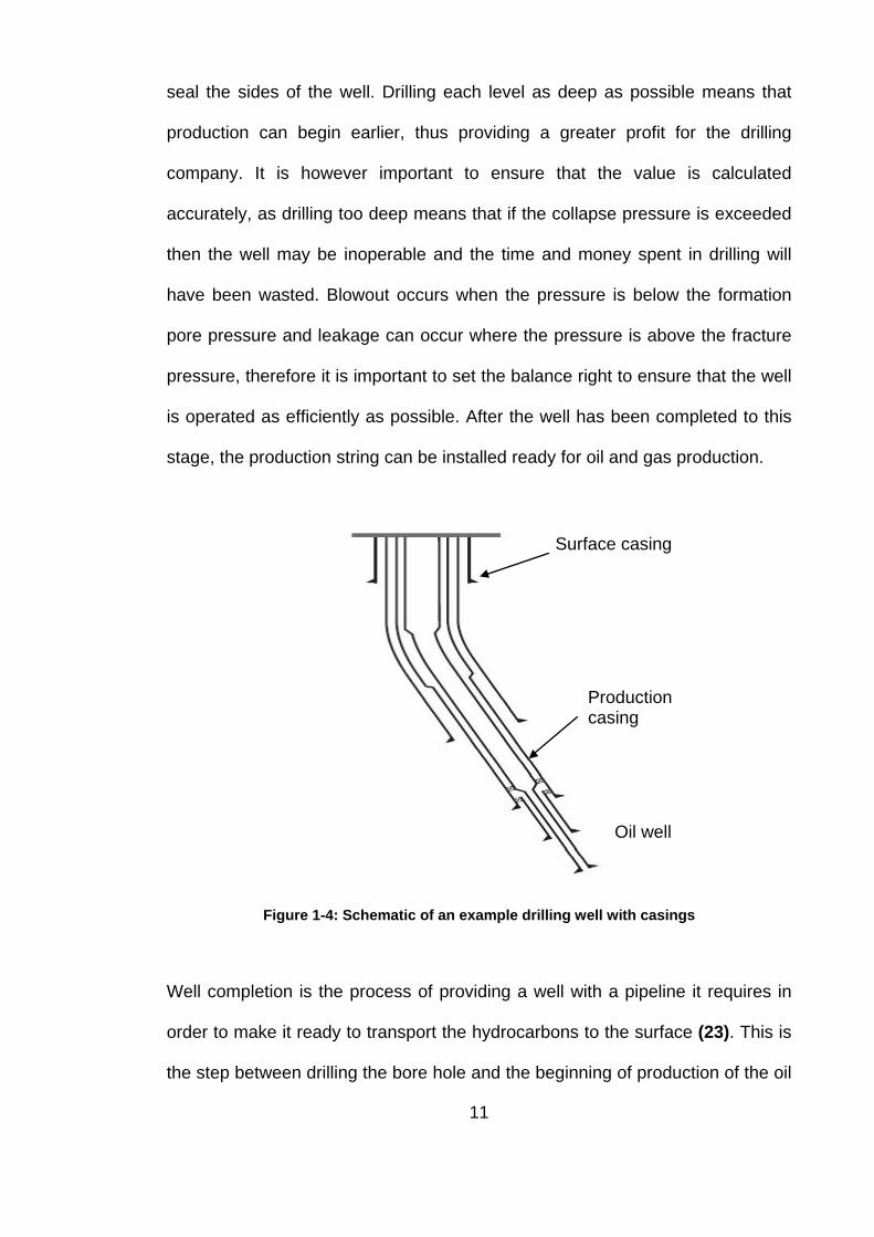
seal the sides of the well. Drilling each level as deep as possible means that
production can begin earlier, thus providing a greater profit for the drilling
company. It is however important to ensure that the value is calculated
accurately, as drilling too deep means that if the collapse pressure is exceeded
then the well may be inoperable and the time and money spent in drilling will
have been wasted. Blowout occurs when the pressure is below the formation
pore pressure and leakage can occur where the pressure is above the fracture
pressure, therefore it is important to set the balance right to ensure that the well
is operated as efficiently as possible. After the well has been completed to this
stage, the production string can be installed ready for oil and gas production.
Figure 1-4: Schematic of an example drilling well with casings
Well completion is the process of providing a well with a pipeline it requires in
order to make it ready to transport the hydrocarbons to the surface (23). This is
the step between drilling the bore hole and the beginning of production of the oil
Production casing
Surface casing
Oil well
11
and gas (24). The type of well is determined by the location of the
hydrocarbons, these can either be vertical or horizontal.
A conventional natural flowing well is shown in Figure 1-4. To produce a well, a
large hole is drilled in the sea bed, which begins with a very large diameter at
the top and reduces in size as the well deepens. This allows the well sides to be
reinforced with concrete to prevent collapse of the side walls. A series of pipes
and couplings (tubing) are attached in a string, inside the well which has already
been completed. This is done using a casing packer fluid, cement, a perforated
casing, and a packer to ensure the sides of the well do not collapse preventing
the removal of hydrocarbons from the well. The tubing (premium tubular pipe
and connection) is run from the well floor to the well head. At the well head,
pressures are maintained and reported by the ‘Christmas trees’. The ‘Christmas
tree’ gets its name from the number of valves and fittings added onto it, as it is
like a set of decorations. These fittings and valves are used to control the flow
and prevent leakage; the devices on the tree can be remotely controlled and
operated safely.
The actual production pipeline consists of pipes, pipe connections, crossover
subs and valves etc. Each pipe connection is usually made up of a threaded
pipe end and a coupling. The pipe end is a male connector and the coupling (so
called ‘box’) end is a female connector. To complete the well, these connections
are fastened together in a bucking unit. Each pipe and coupling connection (be
it a valve, crossover sub or coupling) has a pre-defined torque value associated
with it. It is with this process where the CoF becomes a major issue.
12

Figure 1-5: Completion string of a well without artificial lift (25)
Figure 1-6 shows one type of premium tubular connection. This figure
comprises of two pipe sections of identical design and one coupling. The cross-
sectional image of the connection shows how the pipes and coupling fit
together. Tubing is run down a casted well in order to complete a string ready
for production. The hydrocarbons flow through the production pipe and
connection and therefore they are required to have a sufficient seal at very high
temperatures and pressures. Pipe sections are connected together with
couplings on either end. These are “made-up” by screwing them together using
a predefined torque value. This torque value is pre-determined using an
estimated CoF.
13

Figure 1-6: Premium tubular connection – coupling with two pipes attached (26)
The pipeline is assembled by fastening a pipe into a coupling (in the process
known as make-up) using a bucking unit. Two different versions of these
machines are used onshore (see Figure 1-7) and offshore due to space
utilisation however they work in exactly the same way. An onshore assembly
connects the coupling to the pipe horizontally. Offshore, the pipes are run down
the well and each pipe is connected to the coupling at the well head.
Figure 1-8 shows a premium tubular connection model made up of two pipe
ends and one coupling section. A sectional view of the coupling illustrates the
arrangement shown in more detail.
Metal-to-metal seal
Threads Coupling
Pipe
Pipe
14

Figure 1-7: Bucking unit used for make-up of connections in machine shop
Figure 1-8: Premium tubular connection elements
During the service life of a completion string, premium tubular connections may
be subjected to both high internal and external pressures. Throughout this
period, the connection may also be subject to severe loading conditions
including bending, tension and compression at elevated temperatures. For
Metal-metal seal
15

premium tubular connections to work effectively in such harsh environments,
the connection not only needs to have sufficient strength, but also relies on the
amount of pre-load in the metal-to-metal seal. To maintain the pressure
effectively during the connection’s service life, it is critical that the correct
amount of torque is applied during assembly; thereby overcoming thread
interference and generating the required strain energy in the seal. Seal pre-load
is determined by connection geometry, applied torque and the frictional
properties of the contacting surfaces.
A small proportion of connections fail during their working life. Approximately
two thirds of drilling failures were caused by loose connections (27), where the
majority of losses were caused by galling of threads. Research in the Wall
Street Journal concluded that a gas leak in the North Sea in 2012 had cost its
owners billions of dollars due to lost production, replacement of connections
and unplanned well intervention (28).
The value of fastening torque used to make-up a connection is vital to create a
proficient seal between the coupling and pipe. As the pipeline is secured using
a pre-defined value of torque, this is the main parameter responsible for
ensuring no leakage occurs. The continued search for oil has resulted in deeper
wells being drilled. The resulting increase in the pressures and temperatures
mean that the connection is exposed to increased stresses. It is at this point
that the value of torque becomes most critical. An insufficient value of torque
will mean that there is a poor seal in the connection and leak paths can easily
form. On the opposite side of the spectrum, if the connection is over-torqued,
16
the seal begins to plastically deform, making the connection susceptible to
damage and creating leak paths within the connection. When the connection is
exposed to high pressures and high temperatures, the material finds itself close
to its yield strength, either in tension or compression. This gives opportunity for
leaks to occur, with severe leakages in connections costing a significant amount
due to loss of profit. An example of this is in the Total well platform off the coast
of Elgin, UK. Experts have reported that the cost of closing a well per day
amounted to $1.5 million, with a response call adding another $1 million to the
loss daily (29). The best way to prevent this from happening is to ensure that
the torque value is calculated correctly and accurately. To do this, the CoF has
to be known for all materials, make-up speeds, contact pressures, lubricants,
material properties, surface roughness and other such variables. The current
method of obtaining the CoF is very expensive and requires a large scale
operation along with some interpolation and extrapolation of data to acquire all
necessary values.
The pipe end of the connection is usually peened using a locally available
peening material. This peening process produced a surface with irregular
craters on the surface, and was performed because it was found that the
lubricants used during assembly stuck much more effectively during the sliding
process than a plated surface. It also gave a much more isotropic surface rather
than the unidirectional plated surface, where the lubricant could squeeze out
from the surface much more easily. The media used to peen the steel surfaces
included ceramic particles, stainless steel particles, aluminium oxide particles
17

and also glass particles. This research focussed primarily on the ceramic
peened, stainless steel and aluminium oxide peened surfaces.
1.2.2 Role of friction in a premium tubular connection
The friction coefficient is a very important parameter involved in the make-up of
Oil Country Tubular Goods (OCTG) systems. The pipe and box sections are
screwed together using a pre-defined value of torque. This torque value is
calculated using Duggan's torque equation (30). Duggan’s torque method was
based upon a nut sliding on a bolt. The equation gives the relationship between
the tightening torque and the equivalent end load. It is based on the idea that
“when a bolt is tightened, some of the effort goes in pre-loading the parts (i.e.
the bolts are stretched and the connected members are compressed), and
some goes into overcoming friction both at the threads and at the annular
surface of the bolt head or nut whichever turns” (30).
𝑻𝑻𝑫𝑫𝑫𝑫𝑻𝑻 =𝟒𝟒𝑭𝑭𝒅𝒅𝒎𝒎𝟐𝟐
�𝑻𝑻 + 𝝅𝝅𝒅𝒅𝒎𝒎µ𝒔𝒔𝑻𝑻𝑭𝑭𝒔𝒔𝝅𝝅𝒅𝒅𝒎𝒎 − µ𝑻𝑻𝒔𝒔𝑻𝑻𝑭𝑭𝒔𝒔
+ µ𝑭𝑭𝒅𝒅𝑭𝑭𝒅𝒅𝒎𝒎
� (1.11)
Where,
rP
Connection seal preload
md
Mean pin thread diameter
l
Lead
µ
Coefficient of friction on the thread
𝜇𝜇𝑐𝑐 Coefficient of friction on the shoulder
β
Thread load flank angle
18

cd
Average collar diameter (0.5 x nib thickness)
The loading flank contributes approximately half of Duggan’s torque value
because the force on the seal is equal to the force on the loading flank. As
shown in the equation above, the CoF has a large effect on Duggan’s torque. It
is noted that the CoF on the shoulder µc can differ from that on the thread µ.
This equation was derived by considering the forces acting on an inclined plane
of a bolted joint, which in the case of the premium tubular connection is the helix
angle of the thread; giving the total torque required at the threads. This value
was then added to the torque needed to overcome friction at the annular
bearing surface of the nut or bolt, i.e. the seal of the coupling in the premium
tubular connection.
This is used along with the API RP 5A3 test to acquire CoF from the test
sample. The additional torque caused by the conic shape of the connection is
not incorporated into the equation and has to be calculated separately because
it is not associated with the seal pre-load. By executing the test until yielding
occurred, the pre-load value was then extracted from the geometry and yield
strength, allowing CoF to be estimated. To achieve the wide combinations of
sizes, weights and grades of connections, extrapolation was used as these full
scale tests were not viable to be done for all combinations. The main issue with
interpolating and extrapolating the results to obtain values for every combination
is the unpredictable effects of contact pressure, operating speed and surface
conditions. These effects are not linear and do not always correlate.
19

1.2.3 Current methods for acquiring coefficient of friction
The American Petroleum Institute (API) Recommended Practice (RP) 5A3, 3rd
Edition test protocol provides industry standard methods for testing threaded
connections in the oil and gas industry. From this procedure an estimate for the
friction coefficient in premium tubular connections has been obtained (31). The
test apparatus is made up of a nut and a bolt (bolt shown in Figure 1-9). This
contains three sections: a motor, a torque transducer and a rotation transducer.
Rotation and torque are provided to the samples by the motor. The torque
transducer resists rotation and from this an output signal is produced. The angle
of rotation is calculated using the output signal from the rotational transducer,
where the output signal is proportional to the angle through which the specimen
is rotated. Both the torque and rotational signals are recorded so that there is
one-to-one correlation between the data points. This is used to calculate the
CoF for the system. The test apparatus has geometry which is significantly
different from the premium tubular connection being modelled and this means
that there are discrepancies between the values calculated and the real values
experienced. The load on the shoulder is estimated from the tension of the bolt,
which is inaccurate. A face-to-face contact is expected on the shoulder so that
the contact pressure is much lower than the line contact in the seal of a
premium connection. Furthermore the form of the thread in a premium
connection is far from standard thread form. Therefore some discrepancy is
expected in the distribution of axial load.
20

Figure 1-9: API RP 5A3 (3rd Edition) test piece(31)
Values for the contact pressure on actual premium tubular connections were
taken from robust FE Analysis performed by Hunting Energy Service’s (HES)
Research and Development department. The finite element analysis looked at
the localised pressures on individual nodes, on both the thread and seal
surfaces. Although the nodal pressure values on the threads can be large, there
is no cause for concern regarding yielding of the joints. The section where the
yielding most likely takes place, if any, is within the seal area where very high
localised pressure values are used to maintain seal engagement as shown in
Figure 1-10. Localised yielding is not a catastrophic problem for the integrity of
the structure, but it may cause galling or seizure in the seal contact area and
hence lead to leakage pathways for pressurised oil/gas.
21

Figure 1-10: The Manufacturers FE analysis of seal during make-up (32)
The API test only gives on average a pressure of 20 – 69 MPa (3 – 10 ksi) in
the threads and 206 –413 MPa (30 – 60 ksi) on the loading collar. The true
values in a premium connection are approximately 690 – 2070 MPa (100 – 300
ksi) on the seal and 138 – 690 MPa (20 – 100 ksi) on the thread (32). This API
test generates a thread CoF between 0.05 – 0.07 which is considerably lower
than the true value observed in premium connections for the same lubricant
(31). This is because the contact pressure in API test is much lower compared
to that in the seal of premium tubular connections. This may improve the effect
of hydrodynamic lubrication and reduce the risk of galling in API test and hence
reduces the CoF. Observations of scrapped connections in the field showed
that galling is a usual cause of concern.
Coupling end
Pipe end
Metal-to-metal seal
22
1.2.4 Effect of surface wear and burnishing on CoF
“Wear is the progressive damage of a surface, involving material loss” (1),
which is caused by the contact experienced by two surfaces in relative motion.
It is an unavoidable cohort of friction and occurs in some form each time two
surfaces are in contact with one another. A lubricant can be applied between
two surfaces during contact in order to reduce the wear. Lubrication between
two surfaces creates a gap between them and this means that less material
loss will occur. Miscalculated and unappreciated wear can lead to major
consequences in engineering and it is important that those designing the
moving parts are aware of the problems. It is not only the replacement of parts,
which in itself can be significant, but also the length of time that it takes to
replace them. This replacement process is usually accompanied by machine
downtime resulting in lost production and therefore less profit.
The wear rate is the volume of wearing surface lost per unit sliding distance per
unit time. In dry contact, the wear rate is dependent on the normal load, the
sliding speed, the initial temperature, and the thermal, mechanical and chemical
properties of the materials in contact. As the complexity of wear is so vast, there
are no situations which are entirely understood and no collective method which
can be applied to every case. Minor changes in circumstances that connections
experience can have a major effect on both the wear and the coefficient of
friction of that system. A simple way, used by Williams (1), to differentiate
between mild and severe wear is to examine where the wear rate increases
rapidly with a rising contact pressure. The jump in wear rate is usually very
noticeable and this typically provides a clear distinction of the result of severe
23
wear as opposed to mild wear. Depending on the material types involved in the
contact, and the circumstance to which the surfaces are subjected, influences
the conditions in which this occurs.
It is important to note that the CoF depends on both the properties of the
surfaces in contact and the dynamics of the conditions which the surfaces are
under (33). Coulomb (34) was the first to recognise that the surface roughness
of an object has an effect on the friction between two objects (35). Work done
by Nayak (36) on Gaussian, non-isotropic random surfaces, produced a useful
method of representing the surfaces by equations. It was confirmed that the
CoF is dependent on the surface roughness value and interface properties in
research done by Bengisu et al (33). The authors managed to relate the macro-
scale friction force to the micro-scale forces produced at the areas of true
contact between the surfaces.
Further work by Menezes et al (37) demonstrated that value for the average
CoF in a system is dependent on the mean slope of the surface profile, however
it is not affected by the surface texture of any type of material. Studies by
Sedlacek et al (38) found that in dry testing, the CoF is lower when roughness is
higher; yet in systems with lubrication, the CoF is lower when roughness is
lower. The contradiction in these observations is owing to the different friction
mechanisms in dry or lubricated contact conditions.
24
1.3 Current Research in Tribology of Tubular Connection
Regulatory bodies are abundant in the oil and gas industry to ensure that safety
regulations are adhered to as it is the primary concern. In order to comply with
the regulations, there are a number of standards and specifications which
designs have to satisfy to permit operation down well. In the current
environment, tubing designs are well within the limits to withstand the existing
environmental conditions that they are exposed to, however as the search for oil
and gas goes deeper, the environment becomes more severe. In order to
ensure that designs remain safely within the limitations; companies have to
examine and scrutinise a wider scope of variables, therefore the tribology field
becomes an essential area in the fuller understanding.
1.3.1 Tribology in premium tubular connections
Bradley et al (39) noted the importance of the design being critical to the
reliability of premium tubular connections and threaded casings in High
Pressure High Temperature (HPHT) environments. The authors’ work included
an analysis of the types of thread, thread interference, thread forms, crest-root
designs, seals and service design. The analysis showed that due to the wide
availability of designs and the requirement of a safe environment, it was
important that testing of connections was done accurately and effectively.
As the cost of International Organisation for Standardisation (ISO) testing based
on the ISO 13679 protocol (40) is extremely expensive, it is becoming
increasingly important to attain results for as many different aspects as possible
to reduce costs and the lengths of testing time. An alternative method of testing,
25
on a much smaller scale would therefore benefit any company significantly.
"Modified" ISO testing is already used to prove that components meet the
specified criteria at a reduced cost. These "modified" tests reduce the number
of samples required but increase the number of results gained from testing.
This is done by combining tests looking at different aspects of the internal and
external pressures, with and without bending using the same samples. By
constructing alternative cost-effective test rigs, gaps in testing could be easily
filled. There are a minimum number of tests for combinations of materials which
need to be completed using these ISO tests and therefore interpolation was
used to fill the gaps and extrapolation used to obtain results outside of
conventional limitations. Having a laboratory based test rig allows every
combination to be tested economically but thoroughly.
The main issue in OCTG failures is in connections, where approximately two
thirds of all failures are caused primarily by the connection (41). Guangjie et al
carried out work on premium tubular connection testing using finite element
analysis (27). Guangjie et al split the torque of the system into two main
sections: the friction torque and the deformation torque. The deformation torque
is the one used up when deforming the surfaces of the pipe and coupling of the
connection. Similar to the premium tubular connections examined in this project,
the deformation torque was negligible compared to that of the frictional torque.
In this work the friction torque was obtained by the equation:
𝑻𝑻𝑭𝑭𝑹𝑹 = � � µ𝝈𝝈𝑻𝑻𝑻𝑻𝑭𝑭𝒅𝒅𝑺𝑺𝑲𝑲𝑺𝑺𝑲𝑲𝑲𝑲
(1.12)
26

Where𝑭𝑭 is the radius at the integration point, 𝝈𝝈𝑻𝑻𝑻𝑻 is the normal contact stress, µ
is the friction coefficient obtained from the thread compounds characteristics
and 𝑺𝑺𝑲𝑲 is the contact surface number 𝑲𝑲. The integral is applied to each contact
surface while the summation is to combine the contributions of all surfaces to
the total torque. This allows for the definition of different CoF for each contact
pair. The work looked at the distribution of the equivalent stresses, normal
contact force and of friction in the system. Repeated make-up and break out of
connections affects the taper and this could reduce the pitch diameter of the
pipe end connection.
This concept is similar to Duggan's equation (30). Duggan’s torque equation
permits different CoF value to be defined for the shoulder and the thread to
reflect the different contact regimes, but assumes a constant CoF within each
section. Guangjie’s equation is applied in Finite Element Analysis which
provides continuous stress distribution in the system so that the torque applied
to each element can be combined. This approach allows for the system to be
split into as many sections of contact as necessary. Within each section the
friction coefficient can be regarded as a constant or a continuous function of the
pressure, if known. Therefore, Guangjie’s equation is most useful in cases
where the friction coefficient is sensitive to contact pressure. Nevertheless, the
pre-requisite for this approach is that the friction function is pre-determined.
An attempt was made to understand friction and the forces associated with
tightening conical threaded connections by Baragetti et al (42) in 2003. The
author acquired results by friction testing a full connection. Strain gauges were
27
fitted to locations of the connection which were understood to give values for
axial shoulder pre-load �𝑸𝑸𝑫𝑫𝒑𝒑� and the friction parameter �𝑲𝑲𝑫𝑫𝒑𝒑� was calculated
from the equation below using the pre-defined torque value �𝑴𝑴𝑫𝑫𝒑𝒑� used to
make-up the connection. This method was advantageous because it allowed
the friction to be investigated in real life conditions; nevertheless due to the
costs associated with it, repeated testing could not be undertaken easily and
economically and there was a limit to how many conditions could be
investigated.
𝑴𝑴𝑫𝑫𝒑𝒑 = 𝑲𝑲𝑫𝑫𝒑𝒑𝑸𝑸𝑫𝑫𝒑𝒑 (1.13)
Wittenberghe et al attempted to make modifications to existing pipe and
coupling assembly designs in order to improve fatigue life (43). The reduced
fatigue life was due to the issue of localised stress concentrations initiating
cracks particularly in the thread roots. In order to achieve a better fatigue life,
they endeavoured to change the distribution of load by spreading it more
evenly. In order to do this, they needed to perform testing to understand the
locations of maximum stress. The testing procedure was primarily done using
fatigue experiments. Two-dimensional Finite Element modelling was done for
the connection as a secondary test. The testing procedure comprised of a
universal test machine set up to perform four-point bending tests. This was
more beneficial than a three point bending test as it applied only normal loading
to the material and therefore all damage was caused by the normal stresses
(44). Through repeating the test after alterations had been made, their work was
successful and an improvement in the fatigue life was made. It was established
that under axial load, the section with highest stress concentration was located
28

at the last engaged thread of the pipe, and that this was triggered due to
irregular dispersal of load, which is different to where the maximum stress was
found in the Finite analysis used to establish the maximum stresses in the
design. However, it has to be noted that in the premium tubular connections
investigated in this project, the main loading is carried by the seal and
distributed to all the threads.
1.3.2 Friction and metal-on-metal contact
An understanding of metal-on-metal contact is imperative in many industries.
Meng et al (45) researched the mechanics and lubricating regimes of metal-on-
metal contact in an artificial human hip joint. This is dissimilar to a premium
tubular connection, however there are similarities between the two. Noted in
their work was the importance of controlling the surface roughness to allow
metal-on-metal contact between two surfaces to be successful. The work
concluded that by increasing the contact area (in this case by increasing the
variation rate of the radius of curvature or the size of internal bearing surface)
then the contact area would increase, consequently reducing the contact
pressure, and therefore sequentially increasing the film thickness. This is similar
to that of the premium tubular connection, if the area of contact increased, then
the contact pressure would decrease therefore producing a more even film
thickness.
1.3.3 Friction and surface roughness
Bengisu et al (33) developed a friction model which considered deformation and
adhesion of surface asperities. The paper looked at "true contact" between
29
surfaces and related the micro-scale forces to the macro-scale friction force.
The work was more accurate because it also looked at all areas of contact
between the surfaces and also allowed for the resultant normal forces produced
by the contact on the slopes of the asperities. Until this point no other research
had looked at this in any great depth. The stick-slip phenomenon is a reaction
which occurs in dynamic systems where the objects slide over one another in
an unsteady manner. This occurs when the sliding force is not as high as the
static friction and the samples will not slide over one another until the driving
force is high enough to exceed it. This is most common when the surface
roughness is very high and the authors found that the surface roughness plays
an important role in the stick-slip motion. It was also found that machined
surfaces have the higher tendency to display stick-slip effects than that of non-
stationary roughness surfaces e.g. shot blasted surfaces as used in the majority
of samples tested in this project.
1.3.4 Friction and metallurgy
An investigation into the effect of sliding speed on friction and wear behaviour
was completed by Shafiei and Alpas (46). The authors' work investigated the
frictional behaviour of nickel within an argon atmosphere. Although the testing
conditions were different to those used in this project, some of the procedures
and ideas are similar. The samples used were thick sheets of electrodeposited
nickel and these were polished using a diamond suspension to give a
consistent surface roughness for each test. Both nano-crystalline and micro-
crystalline samples were tested and compared. Values for CoF and wear of the
samples were measured using an off-the-shelf pin-on-disc tribometer. This test
30
method was satisfactory because the authors were not trying to simulate real-
life conditions but were investigating the significance of speed. An optical
interferometric surface profilometer was used to examine the wear mark. The
wear volume and wear rate were calculated using already existent equations. It
was found from the experimentation that for nano-crystalline structures, a large
increase of speed caused an increase in CoF. The authors' assumed that
protective tribo-layers formed on the material surface and these were
responsible for the lower CoF at reduced speeds. At the higher speeds, the
fragments of material removed during sliding were much smaller. This meant
that the smaller particles did not fill the gaps as well as the larger ones and a
defensive layer was not generated, resulting in a higher CoF. For the micro-
crystalline samples, the CoF was impartial to the increased sliding speed.
Farhat et al (47) looked at the effect of grain size on CoF and wear of nano-
crystalline aluminium. The authors' concluded that CoF increases with initial
contact and sliding distance, and then levels out to a constant value until sliding
ceases. CoF was also found to be dependent on grain size: as the grain size
decreased, CoF decreased. Another outcome of the investigation was that CoF
was higher when sliding was carried out in a vacuum. This was because when a
test is undertaken in a vacuum there is an increase in the metallic contact and
this increases CoF value (48). The wear of the system was found to follow a
similar pattern to CoF; as the sliding distance increased, the wear volume
initially increased sharply, and after a certain sliding distance, the rate of growth
of the grain size slowed.
31
1.3.5 Friction and surface topography
Coulomb (34) was the first to recognise that the surface roughness has an
effect on the friction between two objects (35). His work was based upon the
idea that friction was due to the “work done in dragging one surface up the
roughness on surfaces becoming interlocked” (1). However, this was
discredited in the early 19th century by Leslie (49) as he exposed the idea that if
friction is only based on overcoming gravity, then no average change in the
value of elevation of the moving body could result in no friction occurring. This
cannot be true as it has already been proven that some level of friction, even if it
is miniscule, always exists. Leslie concluded that some surfaces in contact
could be moving up whilst others had to be sliding down, which provided an
explanation for the fluctuation of friction.
Work by Greenwood and Williamson (50) in the 1960s investigated contact
between “flat” surfaces. Previous research had already proven that all “flat”
surfaces were rough on some level. This meant that the true contact was
smaller than assumed when the two surfaces appeared to be fully in contact.
The work concluded that the pressure did not affect the separation between the
two surfaces significantly and there was no change in the separation distance
between them when the load was changed. This gave a reason for the inability
to achieve a complete gas-tight seal when using metal-to-metal contact. The
authors also concluded that surfaces which have been “bead-blasted” (i.e.
peened) fit Gaussian distribution very well.
32
The Greenwood and Williamson (GW) model is one of the most established
methods used to predict the ratio of asperity contact. Although changes have
been made to this model throughout years of investigation, the fundamental
features are still widely used and relevant. Greenwood and Williamson's model
was based on the idea that the height of asperities from the mean plane of the
surface has a normal distribution (51). All asperities on the surface were
assumed to be spherical with a constant curvature of 𝑲𝑲𝒔𝒔. The surface is
represented by a matrix of height values which were obtained through statistical
analysis. The method works on the assumption that the asperities deform
elastically, and that each asperity is not affected by the deformation of the
features around it. However this theory was based on elastic contact mechanics
for rough surfaces. It is expected that the contact in the seal of a premium
connection would be quite different. Some plastic deformation of the asperities
would occur due to the considerable contact pressure.
Jackson and Green (52) modelled the elastic contact between rough surfaces
using three very different approaches. The research carried out was to compare
closed form elastic rough surface contact with deterministic models. Closed
form models are those in which the output is obtained by entering data directly
into formulae without changing the input every time. Deterministic models are
where the value is acquired by using the final output as the input values for the
next phase of the test, i.e. no random values can be created. This method is
very time consuming, and therefore if accurate values can be achieved using
the closed form method, then this would be adequate. The authors concluded
that the mesh resolution made a significant difference to the final values. In
33
every test type, the coarser mesh produced a pressure result which had a
difference of about one order of magnitude smaller compared to that of the finer
mesh. This is thought to be caused by the interval between the nodes in the
model. In the coarser model, the force is distributed across a larger area.
However in the finer model the same force is located across a much smaller
surface and therefore as the pressure is equal to the force divided by the area,
the contact pressure is affected accordingly. In each test, the calculated
contact area is smaller for the finer mesh and larger for the coarser mesh, which
is in line with the difference in pressure. For each of the types of test and for
each size of mesh, the predicted contact area is directly proportional to the load
applied. This proves that even though the foundations of the model types are
very different, the outcome remains the same.
Similarly Zavarise et al (53) looked at the relationship between the resolution of
a model and the prediction of the mechanical response of the contact between
surfaces. It was concluded that in cases where random process theory is
applied, the results of the test rely heavily on the lower cut-off length of a
system. Random process theory is where the initial variables are known, but for
each iteration the process does not use the final reading from the previous
phase of the test, therefore creating uncertainties in the resultant values. To
obtain these results, the authors used an entirely numerical approach to model
the topography of the surfaces using statistical models. The materials
represented by these matrices were a zirconium alloy and a stainless steel. It
was shown that as the lower cut off reduces to zero, the slope of the real
contact versus normal load curve decreases to zero for all contact models. The
34
relationship between the preciseness of the model and other properties of the
solution were identified, but the main conclusion drawn from this set of
experiments was that the prediction of contact is extensively dependent on the
deformation regime used in the model and it is the plasticity index which is of
upmost importance.
Sedlacek et al (38) looked at the impact that the surface fabrication has on the
roughness, friction and wear of steel plates. The tribo-testing performed on the
samples used a pin-on-disc measuring device with a ball-on-disc contact. The
surfaces of every test sample underwent a series of checks prior to testing to
ensure that the quality of the surface was consistent. The surface checks were
done using profilometers to check the main roughness parameters including
average surface roughness, root mean square roughness, skewness, Kurtosis,
core peak-to-valley height, reduced peak height and reduced valley depth. The
authors' reasons for testing these in particular were because these show the
greatest differences in values. The effects of different types of surface
treatments were also investigated and various grades of milled, turned, polished
and ground surfaces were examined. Both dry and lubricated tests were
undertaken and different sliding speeds were also tested. The main conclusions
were that in dry tests, there was a lower CoF when the roughness was very
high. However this is only true in severe conditions. In lubricated test set-ups,
CoF is lower when the roughness is low. It was also found that when the sliding
speed was higher, the friction was smaller for both dry and lubricated tests. The
more negative Kurtosis is, the lower the friction is for lubricated tests.
35
Carbone (54) produced a "slightly corrected" method where all spheres were
not of equal curvature. This created asperities whose curvature changed with
varying heights. This method was directly compared with the theories by Bush,
Gibson and Thomas (BGT) (14). The BGT method is a more complicated
technique with a considerable number of calculations involved. Although this
makes the process very expensive and time consuming, it does provide a more
accurate result than the GW method. BGT works by executing an arrangement
of multi-asperity theories. By this method, the true contact area is found to be
linearly correlated to the applied load. Carbone attempted to produce a method
that would be as accurate as the BGT method, but was based upon the theories
of GW. The initial change made was to make the asperities spherical but not of
equal radius; therefore the sphere curvature was dependent on the height. The
new model produced results similar to the BGT findings, and it was also found
that the linear relationship between the contact area and the load was a result
of the varying asperity curvature.
Nayak (36) concluded that for random, isotropic, Gaussian surfaces, the
information required to evaluate the behaviour is contained within “the power
spectral density of the profile in an arbitrary direction”. The height above the
plane reference of the surface is defined as 𝒛𝒛(𝒙𝒙, 𝒚𝒚), where 𝒛𝒛 is a random variable
and (𝒙𝒙,𝒚𝒚) are the Cartesian coordinates in the reference plane. The power
spectral density, 𝝓𝝓, is the Fourier transform of the autocorrelation factor, 𝑹𝑹,
where these are defined to be:
36
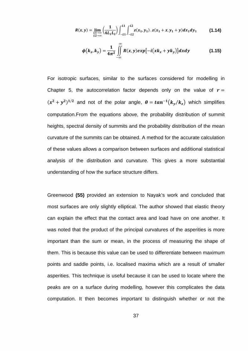
𝑹𝑹(𝒙𝒙,𝒚𝒚) = 𝐥𝐥𝐥𝐥𝐥𝐥𝑳𝑳𝟏𝟏→∞𝑳𝑳𝟐𝟐→∞
�𝟏𝟏
𝟒𝟒𝑳𝑳𝟏𝟏𝑳𝑳𝟐𝟐�� � 𝒛𝒛(𝒙𝒙𝟏𝟏,𝒚𝒚𝟏𝟏)
𝑳𝑳𝟐𝟐
−𝑳𝑳𝟐𝟐
𝑳𝑳𝟏𝟏
−𝑳𝑳𝟏𝟏. 𝒛𝒛(𝒙𝒙𝟏𝟏 + 𝒙𝒙,𝒚𝒚𝟏𝟏 + 𝒚𝒚)𝒅𝒅𝒙𝒙𝟏𝟏𝒅𝒅𝒚𝒚𝟏𝟏 (1.14)
𝝓𝝓�𝒌𝒌𝒙𝒙,𝒌𝒌𝒚𝒚� =𝟏𝟏𝟒𝟒𝝅𝝅𝟐𝟐
�𝑹𝑹(𝒙𝒙,𝒚𝒚)𝑻𝑻𝒙𝒙𝒑𝒑�−𝑻𝑻�𝒙𝒙𝒌𝒌𝒙𝒙 + 𝒚𝒚𝒌𝒌𝒚𝒚��𝒅𝒅𝒙𝒙𝒅𝒅𝒚𝒚∞
−∞
(1.15)
For isotropic surfaces, similar to the surfaces considered for modelling in
Chapter 5, the autocorrelation factor depends only on the value of 𝑭𝑭 =
(𝒙𝒙𝟐𝟐 + 𝒚𝒚𝟐𝟐)𝟏𝟏/𝟐𝟐 and not of the polar angle, 𝜽𝜽 = 𝑻𝑻𝒂𝒂𝑻𝑻−𝟏𝟏�𝒌𝒌𝒚𝒚 𝒌𝒌𝒛𝒛⁄ � which simplifies
computation.From the equations above, the probability distribution of summit
heights, spectral density of summits and the probability distribution of the mean
curvature of the summits can be obtained. A method for the accurate calculation
of these values allows a comparison between surfaces and additional statistical
analysis of the distribution and curvature. This gives a more substantial
understanding of how the surface structure differs.
Greenwood (55) provided an extension to Nayak’s work and concluded that
most surfaces are only slightly elliptical. The author showed that elastic theory
can explain the effect that the contact area and load have on one another. It
was noted that the product of the principal curvatures of the asperities is more
important than the sum or mean, in the process of measuring the shape of
them. This is because this value can be used to differentiate between maximum
points and saddle points, i.e. localised maxima which are a result of smaller
asperities. This technique is useful because it can be used to locate where the
peaks are on a surface during modelling, however this complicates the data
computation. It then becomes important to distinguish whether or not the
37

method supplements the already existent techniques in return for a far more
arduous one, or if a simplified one actually produces results that are sufficiently
accurate.
Work by Buczkowski et al (56) took the analysis one step further and looked at
anisotropic surfaces. Their work concluded that there was a linear relationship
between the applied elastic load and the contact area. This is similar to what is
assumed for isotropic surfaces. In both circumstances, as the load increases,
the surfaces are pushed closer together and as long as the gap between the
surfaces reduces with increasing load, the contact area will increase too.
Although not investigated by the authors for the apparent isotropic surfaces, the
contact stiffness for an anisotropic surface was also found to be proportional to
the normal load. The authors stated the significance of the elastic modulus
which was used to investigate the material properties of both surfaces in
contact. In cases where the surfaces have similar material properties, i.e. where
the Young’s modulus and Poisson’s ratio values are different from one another
especially in the cases where one surface is much more elastic than the other,
the contact (also known as the effective contact modulus) is E* (the plane-strain
modulus). In the case where the materials are the same, the contact modulus is
half of this value.
1.3.6 Lubrication regimes
There are four main types of lubrication: solid lubrication, boundary lubrication,
mixed-film lubrication and hydrodynamic lubrication (57). Figure 1-11 shows the
relationship (according to Stribeck) between the friction coefficient and the
38
lubrication regimes with a lubricant. In the production of the graph, the load and
velocity were kept constant while the viscosity was varied (58). It was found that
the lowest friction coefficient is between the elasto-hydrodynamic and
hydrodynamic lubrication region, which is expected because it is at this point
that the full load is carried by the lubricant. The elasto-hydrodynamic lubrication
involves some elastic deformation in the contact area due to the hydrodynamic
pressure. The minimum friction depends on the materials, contact pressure and
initial surface roughness. The highest friction coefficient shown was observed
during the boundary lubrication phase. This is where the contact load is solely
carried by the boundary layer on the asperity contacts. Often in some cases,
this provides areas of asperity contact which have a thin lubricant film around
the asperities. The friction is a combination of the shearing of the boundary
layer and the lubricant. This is called ‘mixed’ lubrication. The graph was
ciphered using the results of experiments in which the load and speed were
varied in a similar way to the work by Thurston (59).
1.3.6.1 Hydrodynamic lubrication
The likelihood of hydrodynamic lubrication is low for the make-up of a premium
tubular connection, however the initial hypothesis for the project gave rise to the
possibility that due to the low contact pressure in some thread sections such as
the conical surfaces, the surfaces could experience hydrodynamic lubrication. It
was thought that this may explain the low overall CoF used in the API
calculation of torque during the make-up procedure.
39
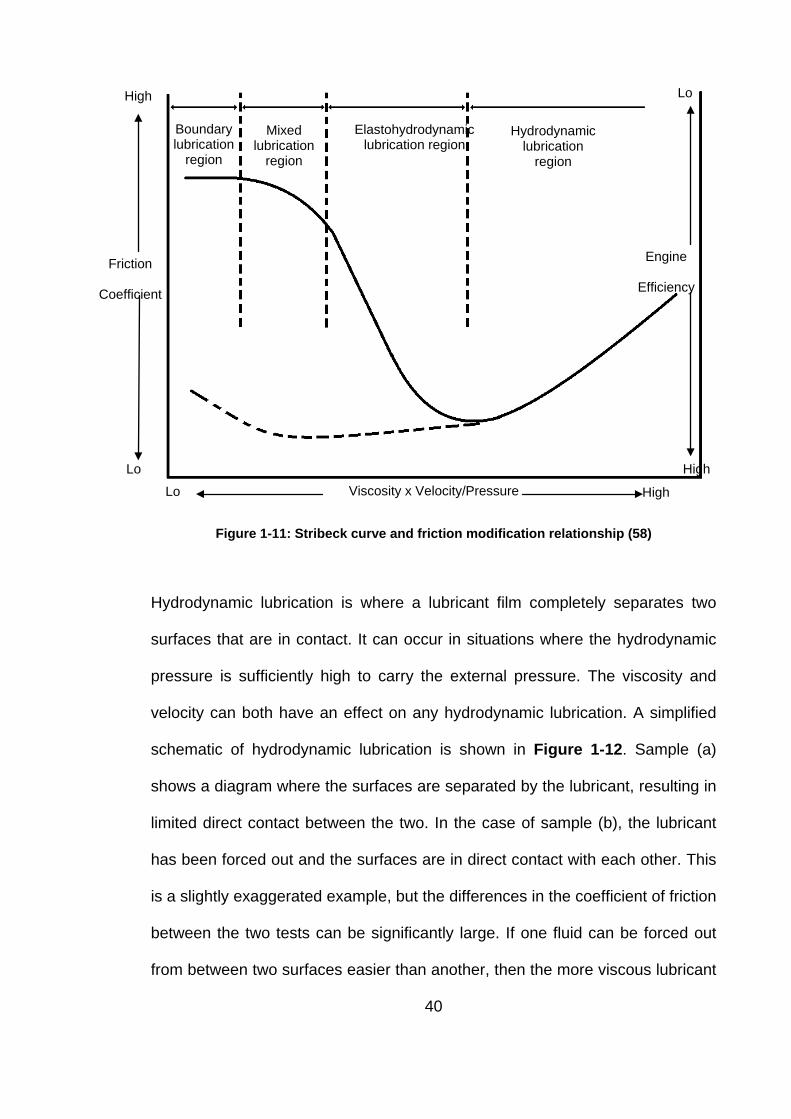
Figure 1-11: Stribeck curve and friction modification relationship (58)
Hydrodynamic lubrication is where a lubricant film completely separates two
surfaces that are in contact. It can occur in situations where the hydrodynamic
pressure is sufficiently high to carry the external pressure. The viscosity and
velocity can both have an effect on any hydrodynamic lubrication. A simplified
schematic of hydrodynamic lubrication is shown in Figure 1-12. Sample (a)
shows a diagram where the surfaces are separated by the lubricant, resulting in
limited direct contact between the two. In the case of sample (b), the lubricant
has been forced out and the surfaces are in direct contact with each other. This
is a slightly exaggerated example, but the differences in the coefficient of friction
between the two tests can be significantly large. If one fluid can be forced out
from between two surfaces easier than another, then the more viscous lubricant
Lo
High
Engine
Efficiency
Lo
High Viscosity x Velocity/Pressure
Friction
Coefficient
Lo
High
Boundary lubrication
region
Mixed lubrication
region
Elastohydrodynamic lubrication region
Hydrodynamic lubrication
region
40

would theoretically create a higher hydrodynamic lubrication effect. Where the
two surfaces fully converge, i.e. no hydrodynamic lubrication is taking place; the
amount of material removed by wear will be significantly higher than where the
two samples are separated by the thin layer.
Figure 1-12: (a) Surfaces separated by lubricant (b) Surfaces in direct contact
Qasim et al (60) modelled the piston skirts in an engine, looking at the effect of
the surface roughness on the lubrication of surfaces at initial engine start-up.
The hydrodynamic film thickness used in the paper was expressed as:
𝒉𝒉 = 𝑪𝑪 + 𝑻𝑻𝑻𝑻(𝑻𝑻)𝑭𝑭𝒐𝒐𝒔𝒔θ + �𝑻𝑻𝒃𝒃(𝑻𝑻) − 𝑻𝑻𝑻𝑻(𝑻𝑻)𝒚𝒚𝑳𝑳𝑭𝑭𝒐𝒐𝒔𝒔θ� (1.16)
Where the piston skirts angle is defined by equation θ = 𝒙𝒙𝑳𝑳� , 𝒙𝒙 and 𝒚𝒚 are
coordinates of the position, 𝑳𝑳 is the piston skirt length, and 𝑻𝑻𝒃𝒃 and 𝑻𝑻𝑻𝑻 are the
acceleration term of piston skirts bottom and top eccentricities respectively.
The hydrodynamic load is carried by this minimum film thickness. The work
concluded that the peak minimum film thickness is found immediately before
combustion and does not change significantly during engine activation when the
engine start-up speed is low.
Teodoriu et al (61) looked at friction considerations in rotary shouldered
threaded connections; another name for a premium tubular connection. The
accepted value of CoF according to the API Standards is 0.07-0.08 and was
(a) (b)
41
obtained through laboratory experiments carried out on different types of metal
particle-containing thread compounds. The lubricants used in the experiments
contained variant amounts of zinc, lead and copper, which is similar to the
constituents of Lubricant B described later in section 2.4. The Farr (62) equation
used to compute the make-up torque (𝑴𝑴) between the pipe and coupling of a
connection is shown:
𝑴𝑴 = 𝑭𝑭𝒗𝒗 �𝟒𝟒𝟐𝟐𝝅𝝅
+𝑹𝑹𝒑𝒑𝑭𝑭𝒐𝒐𝒔𝒔𝒔𝒔
µ𝑻𝑻𝒉𝒉 + 𝑹𝑹𝒔𝒔µ𝒔𝒔� (1.17)
Where 𝑭𝑭𝒗𝒗 is the tension force required in each bolt, 𝑃𝑃is the thread lead, 𝑹𝑹𝒑𝒑 is
the average mean radius from axis of bolt out to point where load is applied to
thread surface, 𝑹𝑹𝒔𝒔 is the mean radius of the nut face, or shoulder and 𝒔𝒔 is half
of the thread angle measured on a plane through the axis.
This equation is similar to that used by Duggan (c.f. Eqn 1.6) in the way that the
torque is highly dependent on the friction coefficient. Similar to Duggan’s
equation, the dimensions of the threaded connection are used in the calculation.
In Duggan’s it is the diameter that is used and in Farr’s it is the radius. Although
the two are very similar, the main difference is in the order of some of the terms.
Two different CoF values are used in the calculation of torque, these are the µ𝒔𝒔,
the CoF in the shoulder and µ𝑻𝑻𝒉𝒉, the thread CoF.
Jeng (63) looked at the effect on friction with changes in height and orientation
of asperities on a surface. Experiments were carried out using a pin-on-disc set-
up on samples which represented a range of heights and directions with
arithmetic average surface roughness (𝑹𝑹a) values between 0.48 and 14.67 µm.
42
As previously stated, the accuracy of such a set-up can be slightly unreliable
when it comes to comparing different testing procedures due to possible
differences in the speed and contact pressure. The overall effect can be
compared satisfactorily and a general trend can be achieved for tests performed
using the same equipment. The results showed that as the load increased, CoF
decreased. The research also concluded that by increasing the speed, CoF
reduced too. A final conclusion of the work was that as the height of the surface
asperities reduced, so too did CoF. This effect of the orientation and heights of
the surface asperities was much larger when the load applied during contact
was higher.
The research of Qiao et al (64) showed the effect of PTFE
(Polytetrafluroethylene) particles on CoF. PTFE is known to produce one of the
lowest values of friction of any type of material. PTFE lubricants are often used
in a contact system to reduce CoF. This works by reducing the adhesion
experienced by the samples when they are in contact, i.e. preventing them from
sticking to one another. A comparison was made between the addition of PTFE
particles to a PEEK (Polyetheretherketone) powder mixed with nano or
micrometer Al2O3 (Aluminium Oxide). An Amsler friction and wear testing
device, which consisted of a rotating ring and a sample, where a load was
applied downwards (see Figure 1-13) was used to obtain wear data. The wear
volume was measured by weighing the sample between tests. This was then
used to calculate the wear coefficient (𝒘𝒘) and friction using the following
equations.
43

Where 𝑽𝑽𝒔𝒔 is the measured volume loss, 𝑿𝑿 is the sliding distance, 𝑳𝑳 is the
applied load, and 𝑹𝑹 is the radius of the steel ring.
Figure 1-13: Amsler friction and wear test rig schematic
Some of the earlier work on modelling hydrodynamic lubrication in rough
surfaces dates back to the 1960s in work done by Ralph Burton (65). His work
entailed using a Fourier series type approximation to model the surface
roughness (66). When the nature of the surface roughness was established to
be random, stochastic approaches began to be used to create a representation
of the surfaces in question. Work by Christensen (communicated by
Christopherson) (67) stated that the value of the maximum pressure depends
on the pressure coefficient of viscosity multiplied by the equivalent Young’s
𝒘𝒘 =𝑽𝑽𝒔𝒔𝑿𝑿.𝑳𝑳
(1.18)
µ =𝑴𝑴𝑹𝑹. 𝑳𝑳
(1.19)
Load, L
Rotating ring
Rotating
Radius, R
Sliding Distance, X
44

modulus. Their work also concluded that at very large pressures, additional load
caused a much larger effect than at lower pressures. This is different from the
assumptions used in this project as in this case the pressure in the system was
assumed to be directly related to the load (see Equations 1.4 to 1.10). Some of
their experiments use balls instead of the cylinders (as used in their compared
theory) and therefore a direct comparison between the experiments is not
possible.
Work done by Ahmed and Sutcliffe (68) looked at identifying surface features of
shot blast steels in cold rolling. Their work produced algorithms which identified
several surface features from a three-dimensional profile of a sample. The
profile was obtained from the three-dimensional images and these were
converted into a matrix which described the surface. The algorithms established
the position of the pits on the surface and also identified the location of the roll
marks. This created a system to estimate the lubrication conditions that the
surface would be exposed to in order to speculate how much oil would be
trapped in features on the face of the material and what effect it would have on
the lubrication. The control of the surface finish can be easily monitored using
this technique, providing a quantifiable approach to inspecting the quality of
surfaces.
1.3.6.2 Boundary lubrication
Boundary lubrication is where the surfaces are so close together that the load is
mainly carried by the asperities with an ultrathin boundary layer (58).
Conventional boundary layers are thought of as solid layers, of which the shear
strength is directly proportional to contact pressure giving rise to a constant 45
coefficient of friction independent of viscosity or sliding velocity as shown in
Figure 1-11. More recent studies suggest that the properties of boundary films
may be more complex than this (69, 70). The properties of the boundary layers
depend on the tenaciousness of the films’ ability to adhere to the surface and
the details of the surface topography. Single molecular layers, such as paraffin
oils, can provide reductions under low contact pressure, but may be depleted
under higher pressure (17). More complex surface films such as CaCO3 in n-
dodecane colloidal solution are very much dependent on the applied pressure
(71, 72). There exists a ‘shakedown’ limit. When loads are in the acceptable
‘shakedown’ or elastic regime, the coefficient of friction falls with increasing
load. Above the ‘shakedown’ limit, the coefficient of friction increases owing to a
contribution from ploughing deformation. The coefficient of friction increases
rapidly with the severity of galling or scuffing which leads to direct metal-to-
metal contact (73-75).
1.4 Knowledge gaps
With the current and future environments that premium tubular connections are
expected to withstand, including high pressures and temperatures, the
expectations of the connections will only increase. The main uncertainty in
current piping research is in the prediction of CoF. Even with the magnitude of
pioneering research presented in this chapter, a method of inputting accurate
CoF for a premium tubular connection does not currently exist. API uses a set
value for every connection, without considering alterations in surface roughness
after initial make-up or in the changes in sliding speed. A method of prediction
would be very beneficial to the current industry in the future. Currently there is
46
limited appreciation for a method of calculation of CoF. However, as
environments become more challenging, future generations will benefit from this
type of research and altering working practices will not seem so costly or time-
consuming. Therefore, there is a need for laboratory research which provides a
method for obtaining values for CoF as well as the wear of the surfaces. Thus
providing foresight into how the connection reacts to being torqued up more
than once, or at different speeds.
There are three distinctive sections in a premium connection. According to the
FEA studies shown above (32), the highest pressure occurs in the seal section.
This is a line contact as shown in Figure 1-10. The pressure is above 600 MPa
which is above the ‘shakedown’ limit so that the lubricant is almost completely
squeezed out of the contact area (75). The dominant lubrication regime is
believed to be boundary lubrication, which is insensitive to sliding speed. The
surface of the seal is usually burnished in the manufacturing process so that it is
smoother than other sections. Some plastic deformation is expected in this
section. Observations in the field also indicate that the surface is burnished after
repeated make and break. Another section is on the loading flanks of the
threads. The loading flanks usually have negative angle in a premium
connection as shown in Figure 1-6. The design of premium connections is to
ensure that the load is distributed to all threads engaged so that the contact
pressure is in the order of 150-500 MPa. This is somewhere below the
‘shakedown’ limit. The surface of the pipe is usually peened so that it is
commonly rougher than other sections. In this case, the contact area was
notably larger and the contact pressure smaller so that the lubricant film in the
47

contact area is allowed to escape through the roughness troughs, leading to a
large fraction of asperity-to-asperity contact. Hence, the friction is a combination
of boundary lubrication and hydrodynamic lubrication which is more sensitive to
sliding speed. The contact pressure on the conical surfaces is the lowest so that
the surface asperities are not removed as quickly as in other sections. It was
initially thought that this section would experience an elasto-hydrodynamic
lubrication effect due to the small pressure it experienced. However, it is not
possible to separate three different sections using full size physical tests. The
lubrication mechanism of each section is not well understood.
It is important to note that it is not only the contact pressure that determines
CoF, but also the details of the surface topography. It is also important to
observe that the surfaces are modified during sliding and repeated make-up as
observed in the field. It is not fully understood how quickly this happens and to
what extent that this changes the CoF. Therefore there is a need to develop a
micromechanical model to understand the relationship between asperity wear
and the implications on the asperity contact, and to establish a friction model
that takes into account the role of lubricant distribution.
1.5 Project aims and objectives
The project was sponsored by Hunting Energy Services (HES), an oil services
company who specialise in premium tubular connections used in the completion
string in the oil and gas industry. HES’s OCTG department provides pipe casing
and premium tubing. Premium tubing is usually connected via premium
connections which consist of a threaded section and a metal-to-metal seal. The
48
metal-to-metal seal provides a liquid and gas tight connection to allow
hydrocarbons to be transported through the connection back to the rig platform.
The threads ensure that the seal is maintained during the high-temperature,
high-pressure environments in which the connections are exposed to during
production.
The initial aim of the collaborative project was to produce a laboratory tool to
measure friction and galling under a wide range of contact conditions, which
mimicked contact conditions in three different sections of a premium connection
to help understand the observations of the role of tribology in the field. The
scope of this project started with the design and manufacture of a test rig based
on existing techniques in order to obtain a range of measurements for CoF with
varying sliding velocity, contact pressure, surface roughness and materials in
contact. Test pieces were manufactured to represent the surfaces in contact for
testing purposes. These samples were exposed to the same procedures that
the pipes and couplings experience in manufacture, producing surfaces that
were comparable with real products. The project was then extended to develop
a model which could predict the surface roughness, friction and wear of
surfaces without such a large amount of physical testing. This reduction of
physical testing has the potential to reduce costs if the outcomes of the
mathematical modelling are accurate.
49

Chapter 2 Design for Measurement of Friction
2.1 Determining the coefficient of friction
2.1.1 Pressure regimes
Contact pressure is an important consideration in the design of a friction test
device. In a premium tubular connection, the most important locations, where
connection contact pressure is of the most interest, are on the seal where the
pin and coupling meet, on the thread cone, and on the thread loading flank. The
contact pressure at each of these sections has a different magnitude and using
Finite Element Analysis (32), the values of each have been estimated.
A premium tubular connection which consists of a metal-to-metal seal relies on
the torque from make-up to seal the connection and prevent leakages. The
torque values are calculated using Duggan's (30) equation relying on accurate
measurements of CoF. An under-torqued connection will not provide a sufficient
seal to prevent leakages from occurring when the pipe is used to extract the oil
from the well. An over-torqued connection is one in which the value used in
make-up is too high and therefore the seal is plastically deformed. This can
result in the occurrence of leak paths in the connection. At current well depths,
the pressures and temperatures that the connections are subjected to are high;
though these are well within the yield strength of the materials in question.
Therefore minor differences in calculated and actual CoF cause limited
problems and will not cause concern. However as the oil reservoirs are
depleting and drilling has to occur at deeper depths, then miscalculations of
50
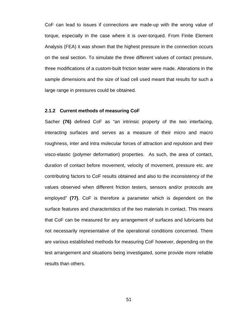
CoF can lead to issues if connections are made-up with the wrong value of
torque, especially in the case where it is over-torqued. From Finite Element
Analysis (FEA) it was shown that the highest pressure in the connection occurs
on the seal section. To simulate the three different values of contact pressure,
three modifications of a custom-built friction tester were made. Alterations in the
sample dimensions and the size of load cell used meant that results for such a
large range in pressures could be obtained.
2.1.2 Current methods of measuring CoF
Sacher (76) defined CoF as “an intrinsic property of the two interfacing,
interacting surfaces and serves as a measure of their micro and macro
roughness, inter and intra molecular forces of attraction and repulsion and their
visco-elastic (polymer deformation) properties. As such, the area of contact,
duration of contact before movement, velocity of movement, pressure etc. are
contributing factors to CoF results obtained and also to the inconsistency of the
values observed when different friction testers, sensors and/or protocols are
employed” (77). CoF is therefore a parameter which is dependent on the
surface features and characteristics of the two materials in contact. This means
that CoF can be measured for any arrangement of surfaces and lubricants but
not necessarily representative of the operational conditions concerned. There
are various established methods for measuring CoF however, depending on the
test arrangement and situations being investigated, some provide more reliable
results than others.
51
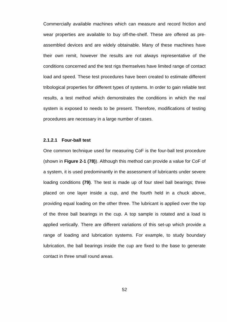
Commercially available machines which can measure and record friction and
wear properties are available to buy off-the-shelf. These are offered as pre-
assembled devices and are widely obtainable. Many of these machines have
their own remit, however the results are not always representative of the
conditions concerned and the test rigs themselves have limited range of contact
load and speed. These test procedures have been created to estimate different
tribological properties for different types of systems. In order to gain reliable test
results, a test method which demonstrates the conditions in which the real
system is exposed to needs to be present. Therefore, modifications of testing
procedures are necessary in a large number of cases.
2.1.2.1 Four-ball test
One common technique used for measuring CoF is the four-ball test procedure
(shown in Figure 2-1 (78)). Although this method can provide a value for CoF of
a system, it is used predominantly in the assessment of lubricants under severe
loading conditions (79). The test is made up of four steel ball bearings; three
placed on one layer inside a cup, and the fourth held in a chuck above,
providing equal loading on the other three. The lubricant is applied over the top
of the three ball bearings in the cup. A top sample is rotated and a load is
applied vertically. There are different variations of this set-up which provide a
range of loading and lubrication systems. For example, to study boundary
lubrication, the ball bearings inside the cup are fixed to the base to generate
contact in three small round areas.
52
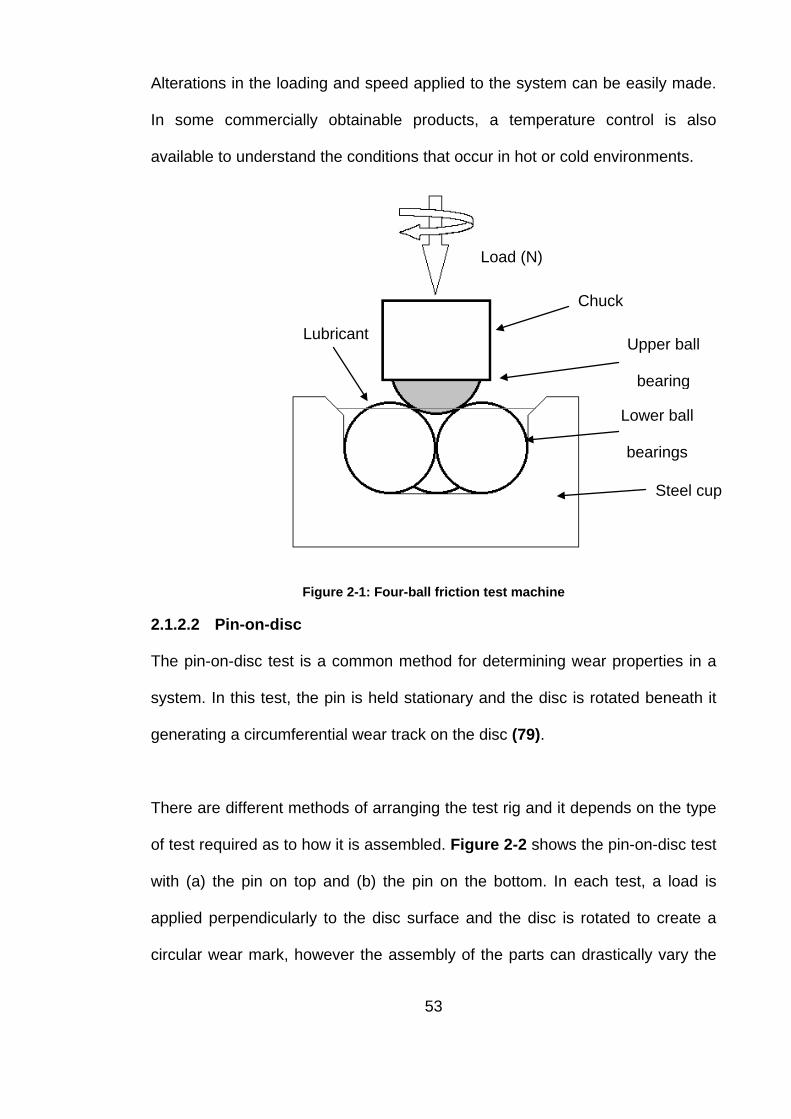
Alterations in the loading and speed applied to the system can be easily made.
In some commercially obtainable products, a temperature control is also
available to understand the conditions that occur in hot or cold environments.
Figure 2-1: Four-ball friction test machine
2.1.2.2 Pin-on-disc
The pin-on-disc test is a common method for determining wear properties in a
system. In this test, the pin is held stationary and the disc is rotated beneath it
generating a circumferential wear track on the disc (79).
There are different methods of arranging the test rig and it depends on the type
of test required as to how it is assembled. Figure 2-2 shows the pin-on-disc test
with (a) the pin on top and (b) the pin on the bottom. In each test, a load is
applied perpendicularly to the disc surface and the disc is rotated to create a
circular wear mark, however the assembly of the parts can drastically vary the
Chuck
Upper ball
bearing
Lower ball
bearings
Steel cup
Lubricant
Load (N)
53

results of the test. When the pin is on top (a), the removed material remains on
the surface of the disc and as the number of cycles becomes greater, this
volume of debris increases and causes abrasive wear. In the case where the
pin is on the bottom (b), the debris removed in the wear process falls off due to
gravity. This means that the wear test is not identical in both situations as there
is abrasive wear occurring. This makes it imperative that when CoF results are
being compared from external practices, the type of test is known to give a fair
and reliable comparison. Another disadvantage of the test is that if the pin and
disc are not aligned properly, the pressure applied on the surface will not be
accurate and this has the ability to cause variances in testing procedures.
Figure 2-2: Pin-on-disc test (a) pin on top (b) pin on bottom
Podgornik et al (80) reviewed various laboratory friction test methods. It was
established that the simplest and most extensively used procedure for general
friction testing was the pin-on-disc technique. However, to obtain a new contact
surface each time, the location of the pin had to be adjusted for each test
making the testing procedure very time consuming. Further, a rounded pin is
Rotating base
Rotating top
Load applied downwards
Load applied upwards
54

required in order to generate a high contact pressure representative of premium
connection. Consequently the contact pressure can change significantly when
there is wear on the rounded pin. There are also discrepancies in sliding speed
and sliding distance between the test and the connection during make-up. The
operating sliding speed of commercial pin-on-disc machines usually ranges
between 0.05 and 10 m/s (81), which is significantly higher than the speed
concerned with a premium tubular connection assembly make-up, which is
within the range of 3 mm/s to 50 mm/s (82). Another issue is that the sliding
distance in these tests is at least tens of metres each run which is much larger
than what occurs in tubular connections.
2.1.2.3 API test method
As described in 0, the APIRP 5A3 (3rd Edition) document describes the
recommended practice for obtaining frictional data in threaded connections (31).
The test rig contains a nut rotating on a bolt assembly (see Figure 1-9) where
the bolt is rotated into the stationary nut until a specific pre-load is attained. CoF
is extracted from the torque data and the estimated contact pressure from the
angle of rotation. Although this is a widely used testing procedure for threaded
components, it lacks comparativeness between external conditions including
contact pressure and the material finish on the seal section. The contact
pressure generated in this test method is only 200 to 400 MPa (30 - 65 ksi) on
the loading collar and below 260 MPa (40 ksi) on the threads. This is
significantly lower than the values of contact pressure on the threaded section
of the connection which were estimated using FEA. In this project, the seal
pressure was found to be between 689 – 2068 MPa (100 – 300 ksi) [see Figure
2-3]. The pressure was found to be different at two sections of the thread and 55
both were required to gain a full perspective of the contact pressures between
the surfaces during make-up. The loading flank of the thread, i.e. on the leading
edge of the thread was found to be subjected to 130 - 480 MPa (20 – 70 ksi).
The cone of the thread was subjected to less than 130 MPa (20 ksi). Therefore
CoF data obtained using this method may be representative of that for the cone
and thread sections, but questionable for the seal due to the discrepancy in the
contact pressure.
Figure 2-3: Locations of pressure in a premium tubular connection
2.1.2.4 Conical pin on box
Conical pipe-on-box tests with coincident tapers were used by Carper et al (83)
to measure the friction coefficient. It is a line contact in circumference of the
conical surfaces. The box was rotated whilst the normal load was increased
linearly. CoF was obtained by measuring the axial force and the torque applied.
To produce the necessary contact pressure, a large axial force was required
and this meant that a large experimental device was needed. This is perhaps
the most representative of the contact conditions in the seal but the cost is
comparable to that of full size tests. Therefore the range of tests is very limited.
56

2.1.3 Design and construction of the test rig
Since CoF is dependent on the system being tested, it is imperative that the
experiments carried out are representative of real contact conditions. The main
parameters of interest are the velocity, sliding distance, contact pressure,
surface conditions and lubricant which all have the potential to cause changes
to CoF obtained.
Similar to work by Le et al (73, 84), a reciprocal sliding test rig was designed
and manufactured to obtain a sliding friction measuring device, capable of
achieving a large range of pressures to simulate various sections of the
surfaces in contact during the make-up of a premium tubular connection. As
shown in Figure 2-4, two samples of pre-determined material type and surface
finish were held in holders positioned perpendicular to one another. A circular
contact between two cross cylinders is generated. The combinations, which
include the sample types and lubricants used, were based upon circumstances
that represent the actual field conditions which premium connections
experience during oil production. The samples slide over one another linearly
starting with a minimum pressure 0 MPa (0 ksi) and moving to maximum
pressure (determined by angle of tilt table and type of samples) before returning
back to zero. This was done using a motorised table which was controlled by a
specifically written program in Aerotech Soloist, detailed in Appendix 1. Figure
2-5 shows the configuration of the samples at the minimum and maximum
pressures.
57
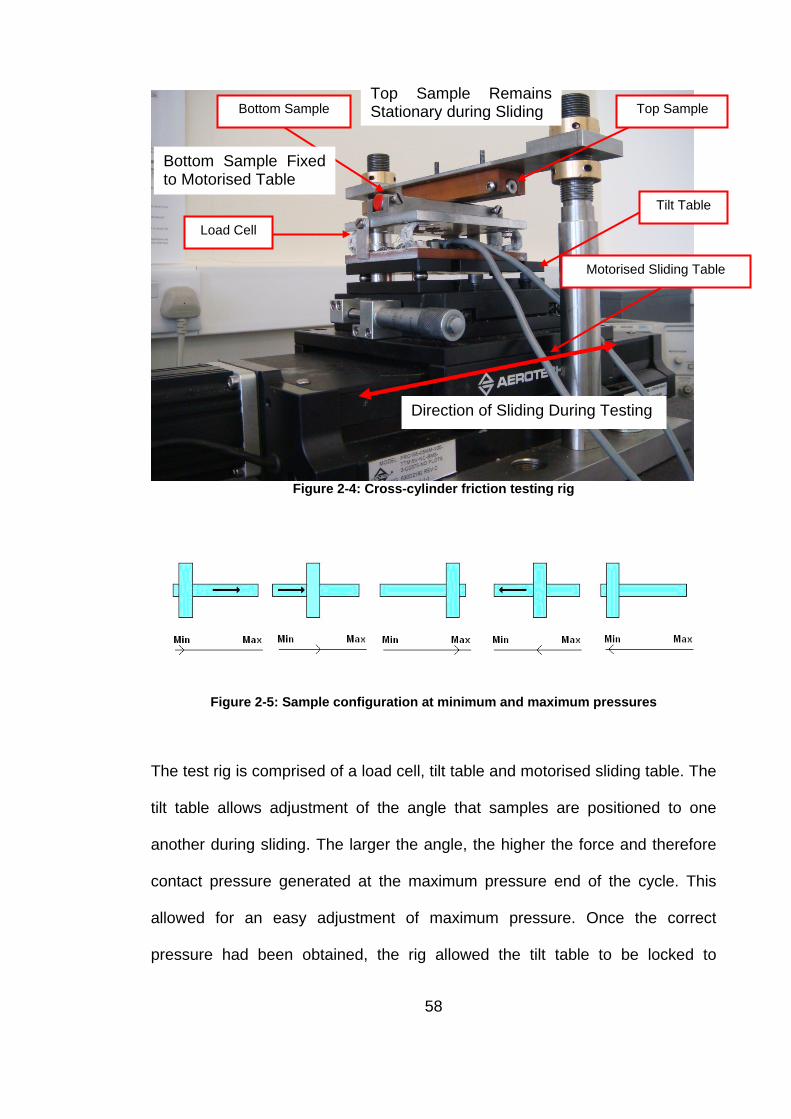
Figure 2-4: Cross-cylinder friction testing rig
Figure 2-5: Sample configuration at minimum and maximum pressures
The test rig is comprised of a load cell, tilt table and motorised sliding table. The
tilt table allows adjustment of the angle that samples are positioned to one
another during sliding. The larger the angle, the higher the force and therefore
contact pressure generated at the maximum pressure end of the cycle. This
allowed for an easy adjustment of maximum pressure. Once the correct
pressure had been obtained, the rig allowed the tilt table to be locked to
Top Sample
Load Cell
Tilt Table
Bottom Sample
Motorised Sliding Table
Direction of Sliding During Testing
Top Sample Remains Stationary during Sliding
Bottom Sample Fixed to Motorised Table
58

maintain the same contact pressure for future tests to ensure consistency and
repeatability of testing.
Due to the large pressure range involved in a premium tubular connection, 20
MPa to 2 GPa (3 and 300 ksi), three different regimes were designed to allow
the pressures to be investigated. Three sets of samples of different geometries
were manufactured to represent the surfaces of the pipe-end and coupling
sections of the connection. Each different regime employed a cross-cylinder
configuration with curved test samples. The curved shape of the test samples
meant that the contact was point contact. The ‘pins’ (see assembly in Figure
2-4) used in Regime 1 for pressures between 620 MPa – 2 GPa (90 and 300
ksi), were manufactured with a diameter of 12 mm and the ‘coupon’ samples
(see Figure 2-8), used in Regime 2 and 3, were cut from actual pipe samples
(see Figure 2-5). For Regime 2 the samples had a diameter of 120 mm and for
Regime 3 samples with a diameter of 168 mm were used. The maximum
pressure for both was achieved by applying a normal force of up to 500 N to the
samples and load cell.
Figure 2-6: Regime 1 (P = 620 – 2000 MPa or 90 – 300 ksi) perpendicular pin test
Diameter = 12 mm
Bottom sample – linearly slides during testing
Top sample – stationary during testing
59
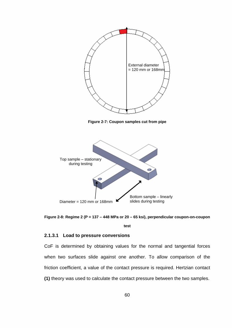
Figure 2-7: Coupon samples cut from pipe
Figure 2-8: Regime 2 (P = 137 – 448 MPa or 20 – 65 ksi), perpendicular coupon-on-coupon
test
2.1.3.1 Load to pressure conversions
CoF is determined by obtaining values for the normal and tangential forces
when two surfaces slide against one another. To allow comparison of the
friction coefficient, a value of the contact pressure is required. Hertzian contact
(1) theory was used to calculate the contact pressure between the two samples.
Bottom sample – linearly slides during testing
Top sample – stationary during testing
Diameter = 120 mm or 168mm
External diameter = 120 mm or 168mm
60

In general, the pressure is quantified as the force divided by the sample contact
cross-sectional area. Due to the complexity of the shape of the area of contact
in the test assembly, a more complicated formula had to be used to calculate
this pressure value. The two curved surfaces in contact create a shape that can
be compared to a semi-elliptical form. This pressure distribution can be
extended into the third dimension, and so the analysis made applicable to the
contact of two spheres (according to Williams (1)), giving the contact pressure
to be:
𝒑𝒑(𝒙𝒙) = 𝒑𝒑𝟎𝟎�𝟏𝟏 − �𝒙𝒙𝟐𝟐 𝒂𝒂𝟐𝟐� �
𝒑𝒑(𝑭𝑭) = 𝒑𝒑𝟎𝟎�𝟏𝟏 − �𝑭𝑭𝟐𝟐 𝒂𝒂𝟐𝟐� �, where 𝑭𝑭𝟐𝟐 = 𝒙𝒙𝟐𝟐 + 𝒚𝒚𝟐𝟐
(2.1)
Where𝒂𝒂 is the radius of the contact circle, 𝒑𝒑𝟎𝟎 is the peak pressure, and 𝒙𝒙, 𝒚𝒚 and
𝒛𝒛 are Cartesian coordinates of the area of interest. 𝑾𝑾, the total load on the
contact spot, is calculated using:
𝑾𝑾 = � 𝟐𝟐𝝅𝝅𝑭𝑭𝒑𝒑(𝑭𝑭)𝒂𝒂
𝟎𝟎𝒅𝒅𝑭𝑭 =
𝟐𝟐𝟑𝟑𝒑𝒑𝟎𝟎𝝅𝝅𝒂𝒂𝟐𝟐 (2.2)
The mean pressure, 𝒑𝒑𝒎𝒎 = 𝑾𝑾𝝅𝝅𝒂𝒂𝟐𝟐� , and rearranged gives an expression in terms
of the peak pressure.
𝒑𝒑𝒎𝒎 =𝟐𝟐𝟑𝟑𝒑𝒑𝟎𝟎 (2.3)
The deflections of the surfaces, both inside and outside the contact area (due to
pressure loading) are consistent with:
When |𝑭𝑭| = 𝒂𝒂 , 𝒘𝒘𝒛𝒛𝟏𝟏 + 𝒘𝒘𝒛𝒛𝟐𝟐 = 𝜟𝜟 − 𝑭𝑭𝟐𝟐
𝟐𝟐𝑹𝑹
When |𝑭𝑭| > 𝑎𝑎 , 𝒘𝒘𝒛𝒛𝟏𝟏 + 𝒘𝒘𝒛𝒛𝟐𝟐 > 𝛥𝛥 − 𝑭𝑭𝟐𝟐
𝟐𝟐𝑹𝑹
(2.4)
61
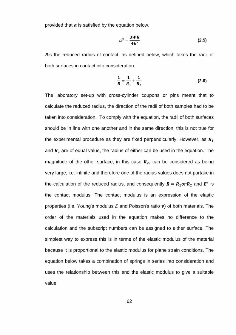
provided that 𝒂𝒂 is satisfied by the equation below.
𝒂𝒂𝟑𝟑 =𝟑𝟑𝑾𝑾𝑹𝑹𝟒𝟒𝑬𝑬∗
(2.5)
𝑹𝑹is the reduced radius of contact, as defined below, which takes the radii of
both surfaces in contact into consideration.
𝟏𝟏𝑹𝑹
=𝟏𝟏𝑹𝑹𝟏𝟏
+𝟏𝟏𝑹𝑹𝟐𝟐
(2.6)
The laboratory set-up with cross-cylinder coupons or pins meant that to
calculate the reduced radius, the direction of the radii of both samples had to be
taken into consideration. To comply with the equation, the radii of both surfaces
should be in line with one another and in the same direction; this is not true for
the experimental procedure as they are fixed perpendicularly. However, as 𝑹𝑹𝟏𝟏
and 𝑹𝑹𝟐𝟐 are of equal value, the radius of either can be used in the equation. The
magnitude of the other surface, in this case 𝑹𝑹𝟐𝟐, can be considered as being
very large, i.e. infinite and therefore one of the radius values does not partake in
the calculation of the reduced radius, and consequently 𝑹𝑹 = 𝑹𝑹𝟏𝟏𝒐𝒐𝑭𝑭𝑹𝑹𝟐𝟐 and 𝑬𝑬∗ is
the contact modulus. The contact modulus is an expression of the elastic
properties (i.e. Young's modulus 𝑬𝑬 and Poisson's ratio 𝒗𝒗) of both materials. The
order of the materials used in the equation makes no difference to the
calculation and the subscript numbers can be assigned to either surface. The
simplest way to express this is in terms of the elastic modulus of the material
because it is proportional to the elastic modulus for plane strain conditions. The
equation below takes a combination of springs in series into consideration and
uses the relationship between this and the elastic modulus to give a suitable
value.
62
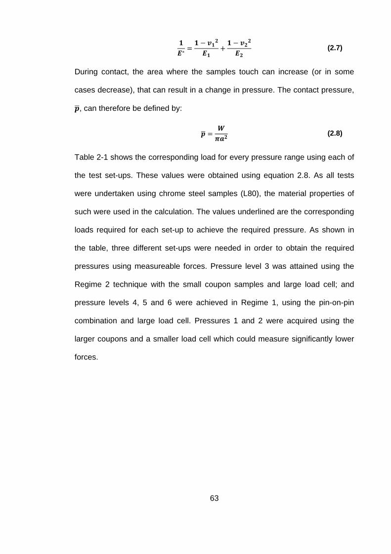
𝟏𝟏𝑬𝑬∗
=𝟏𝟏 − 𝒗𝒗𝟏𝟏𝟐𝟐
𝑬𝑬𝟏𝟏+𝟏𝟏 − 𝒗𝒗𝟐𝟐𝟐𝟐
𝑬𝑬𝟐𝟐 (2.7)
During contact, the area where the samples touch can increase (or in some
cases decrease), that can result in a change in pressure. The contact pressure,
𝒑𝒑�, can therefore be defined by:
𝒑𝒑� =𝑾𝑾𝝅𝝅𝒂𝒂𝟐𝟐
(2.8)
Table 2-1 shows the corresponding load for every pressure range using each of
the test set-ups. These values were obtained using equation 2.8. As all tests
were undertaken using chrome steel samples (L80), the material properties of
such were used in the calculation. The values underlined are the corresponding
loads required for each set-up to achieve the required pressure. As shown in
the table, three different set-ups were needed in order to obtain the required
pressures using measureable forces. Pressure level 3 was attained using the
Regime 2 technique with the small coupon samples and large load cell; and
pressure levels 4, 5 and 6 were achieved in Regime 1, using the pin-on-pin
combination and large load cell. Pressures 1 and 2 were acquired using the
larger coupons and a smaller load cell which could measure significantly lower
forces.
63
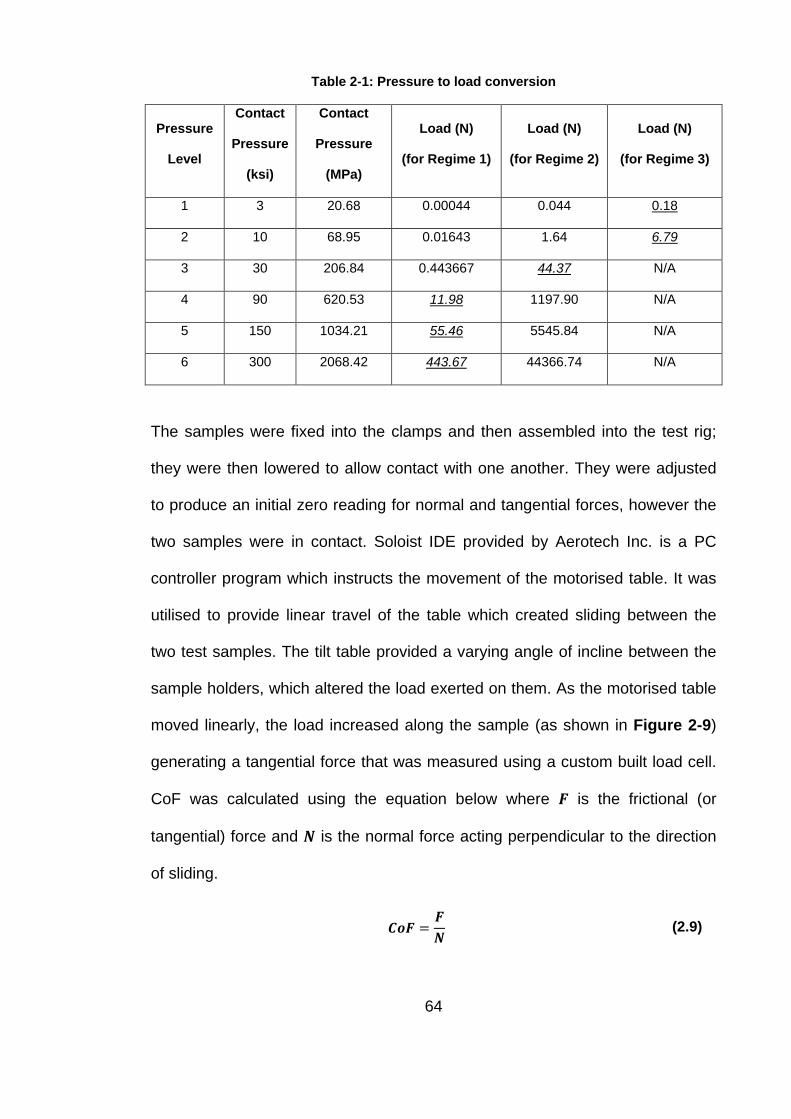
Table 2-1: Pressure to load conversion
Pressure
Level
Contact
Pressure
(ksi)
Contact
Pressure
(MPa)
Load (N)
(for Regime 1)
Load (N)
(for Regime 2)
Load (N)
(for Regime 3)
1 3 20.68 0.00044 0.044 0.18
2 10 68.95 0.01643 1.64 6.79
3 30 206.84 0.443667 44.37 N/A
4 90 620.53 11.98 1197.90 N/A
5 150 1034.21 55.46 5545.84 N/A
6 300 2068.42 443.67 44366.74 N/A
The samples were fixed into the clamps and then assembled into the test rig;
they were then lowered to allow contact with one another. They were adjusted
to produce an initial zero reading for normal and tangential forces, however the
two samples were in contact. Soloist IDE provided by Aerotech Inc. is a PC
controller program which instructs the movement of the motorised table. It was
utilised to provide linear travel of the table which created sliding between the
two test samples. The tilt table provided a varying angle of incline between the
sample holders, which altered the load exerted on them. As the motorised table
moved linearly, the load increased along the sample (as shown in Figure 2-9)
generating a tangential force that was measured using a custom built load cell.
CoF was calculated using the equation below where 𝑭𝑭 is the frictional (or
tangential) force and 𝑵𝑵 is the normal force acting perpendicular to the direction
of sliding.
𝑪𝑪𝒐𝒐𝑭𝑭 =𝑭𝑭𝑵𝑵
(2.9)
64
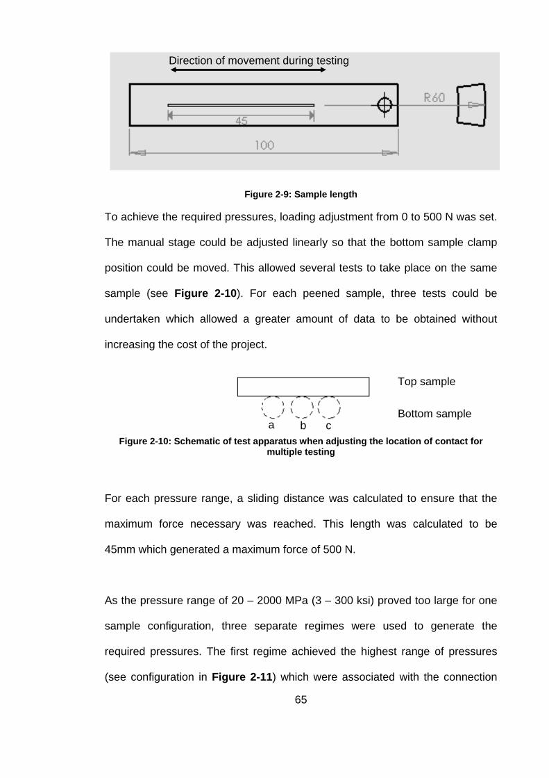
Figure 2-9: Sample length
To achieve the required pressures, loading adjustment from 0 to 500 N was set.
The manual stage could be adjusted linearly so that the bottom sample clamp
position could be moved. This allowed several tests to take place on the same
sample (see Figure 2-10). For each peened sample, three tests could be
undertaken which allowed a greater amount of data to be obtained without
increasing the cost of the project.
Figure 2-10: Schematic of test apparatus when adjusting the location of contact for multiple testing
For each pressure range, a sliding distance was calculated to ensure that the
maximum force necessary was reached. This length was calculated to be
45mm which generated a maximum force of 500 N.
As the pressure range of 20 – 2000 MPa (3 – 300 ksi) proved too large for one
sample configuration, three separate regimes were used to generate the
required pressures. The first regime achieved the highest range of pressures
(see configuration in Figure 2-11) which were associated with the connection
Top sample
a b c Bottom sample
Direction of movement during testing
65

seal. This used a pin-on-pin arrangement and pressures between 206 – 2000
MPa (30 – 300 ksi) [Regime 1] were generated using a normal force of 5-500 N.
Following high pressure tests, it was found that the test data was only valid and
reliable for pressures between 620 – 2000 MPa (90 – 300 ksi) due to the initial
period of acceleration of the motorised table. This unreliable residual strain was
removed from the results before plotting CoF graphs. The tilt table provided a
variable incline for the horizontal surface of the load cell. Test pins/coupons
were placed in a sample holder perpendicular to one another; the motorised
table slid the samples at a right angle to create an area of contact from which
CoF could be calculated.
The load cell was designed to provide both normal force and tangential force
output voltages, and these were used to calculate CoF. The angle of incline of
the samples altered the force exerted on the two samples during the increase in
sliding distance. As the angle of incline increased, the higher end of the sample
became higher up in the test set-up and therefore this meant that the force
increased proportionally. The stiffness of the set-up comes directly from the
strength of the load cell legs, therefore creating a method of altering the
maximum allowable pressure during the testing. A larger angle of incline
created a higher normal load between the two samples, allowing adjustment in
the test set-up. The Aerotech motorised table with controller is capable of
speeds of up to 100 mm/s and moves a linear distance of up to 45 mm (see
Figure 2-9). For each set of tests, velocities of 3 mm/s, 15 mm/s and 50 mm/s
were evaluated. The sliding distance was maintained for every test to ensure
66

that the maximum pressure was kept consistent. Regime 1 is representative of
connection seal engagement, from initial contact to shoulder abutment (82).
Regime 2 (shown in Figure 2-8) employed a perpendicular coupon-on-coupon
configuration which produced a lower pressure range i.e. 137 – 448 MPa (20 –
65 ksi). The samples were held in clamps positioned perpendicular to one
another; the view shown in Figure 2-11 shows the set-up before any load was
applied. The section of the coupon that is visible is the side that experiences the
higher pressures during the test. The forces generated in this set-up were
similar to that of Regime 1. However due to the larger radius of the sample and
therefore larger contact area, the contact pressure range was lower (from
Figure 2-11) and provided CoF results for pressures between 137 – 483 MPa
(20 -70 ksi).
Figure 2-11: Regime 2 friction test set-up
67
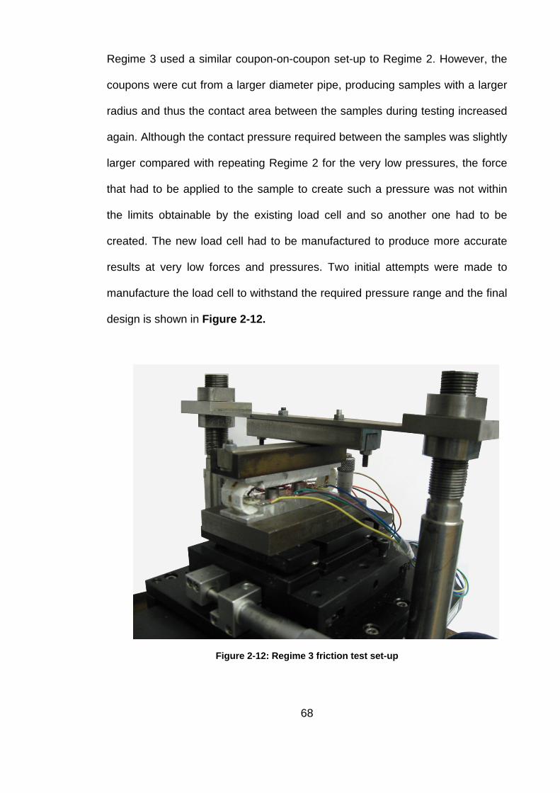
Regime 3 used a similar coupon-on-coupon set-up to Regime 2. However, the
coupons were cut from a larger diameter pipe, producing samples with a larger
radius and thus the contact area between the samples during testing increased
again. Although the contact pressure required between the samples was slightly
larger compared with repeating Regime 2 for the very low pressures, the force
that had to be applied to the sample to create such a pressure was not within
the limits obtainable by the existing load cell and so another one had to be
created. The new load cell had to be manufactured to produce more accurate
results at very low forces and pressures. Two initial attempts were made to
manufacture the load cell to withstand the required pressure range and the final
design is shown in Figure 2-12.
Figure 2-12: Regime 3 friction test set-up
68

2.1.4 Load cells
2.1.4.1 Large pressure load cell
Both load cells were of similar design. The large pressure load cell had four
fixing points, which made calibration and reducing the effect of crossover more
difficult compared to the same process in the two-legged small pressure load
cell. Crossover was an effect caused from minor differences in the load cell
legs’ thicknesses and other unavoidable defects. The crossover effect meant
that even when a load was applied to the middle of the top plate, registering
what should have been equal loading on each leg; different values of voltage
were measured. This irregularity in values meant that something had to be done
to counteract these issues and this was done during the data processing of
strain gauge readings.
Both load cells consisted of an arrangement of strain gauges, which could be
assembled into tension or compression depending on how the equipment was
loaded. Figure 2-13 shows the location of the eight strain gauges in the low
pressure load cell, and half of the strain gauges on the high pressure one. In the
case of the high pressure load cell, four strain gauges were positioned on each
of the four load cell legs. When a normal load was applied to top plate, gauge
(a) stretched in tension and gauge (b) experienced a value of equal magnitude
of compression in the opposite direction. This meant that in order to verify that
the geometry and position of the legs was accurate, the two should be equal in
magnitude and opposite in sign when a force was applied to the top plate. This
extends to the other legs too as it should experience the same loading on
gauges (e) and (f), provided that the weight was positioned in the middle of the
69

load cell. These strain gages were arranged in one full bridge to measure the
normal force. Gauges (c) and (d) were used to measure the force in the
tangential direction when the linear motor applied a force in the horizontal
direction. In this case, gauges (c) and (d) recorded equal magnitude and
opposite sign values of strain as did gauges (g) and (h). Therefore strain gage
c, d, g, h were arranged in another full bridge to measure the tangential force.
The same can be said of the other set of gauges on the two extra legs on the
large pressure load cell. As the bottom plate was held down, the top section
was distorted by the movement.
Figure 2-13: Load cell strain gauge positions
Before manufacture, an initial assessment had to be done to ensure that the
load cell could withstand the forces required to achieve the contact pressures
between the surfaces. This evaluation also ensured that the load cell was
produced from an appropriate material. To do this, Finite Element Analysis
performed using ANSYS and SolidWorks predicted the strains involved when
applying the force to the top surface of the leg. It was also imperative that
enough strain was produced in the load cell to ensure that it would register a
response to the testing process. The load cell was chosen to be made from
a e b f
c g
d h
Tangential Force Normal Force
70
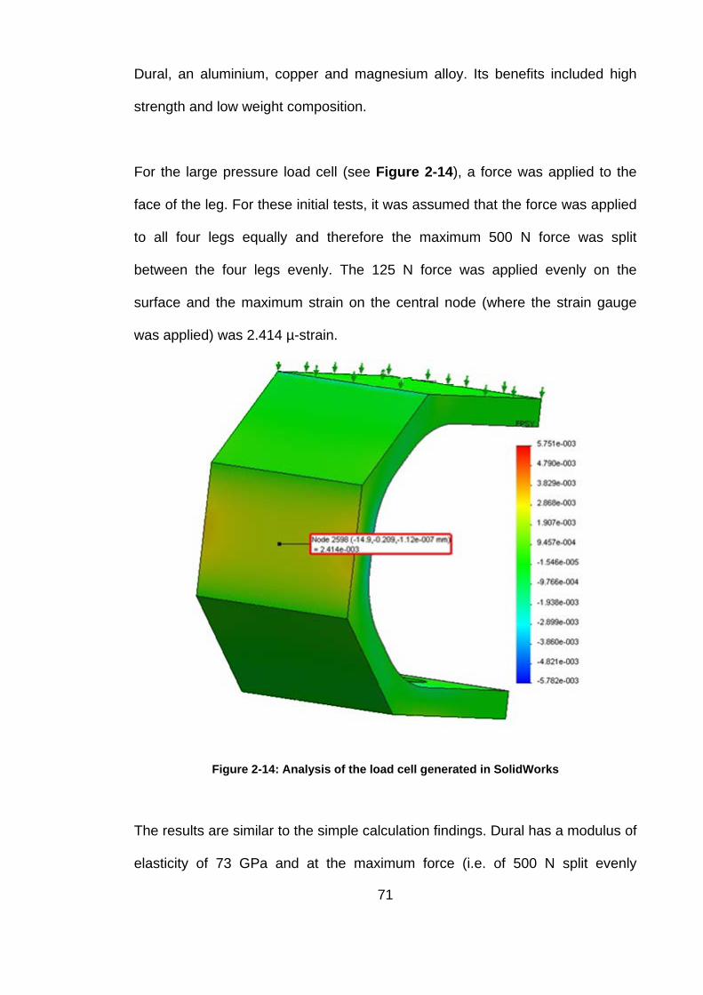
Dural, an aluminium, copper and magnesium alloy. Its benefits included high
strength and low weight composition.
For the large pressure load cell (see Figure 2-14), a force was applied to the
face of the leg. For these initial tests, it was assumed that the force was applied
to all four legs equally and therefore the maximum 500 N force was split
between the four legs evenly. The 125 N force was applied evenly on the
surface and the maximum strain on the central node (where the strain gauge
was applied) was 2.414 µ-strain.
Figure 2-14: Analysis of the load cell generated in SolidWorks
The results are similar to the simple calculation findings. Dural has a modulus of
elasticity of 73 GPa and at the maximum force (i.e. of 500 N split evenly
71
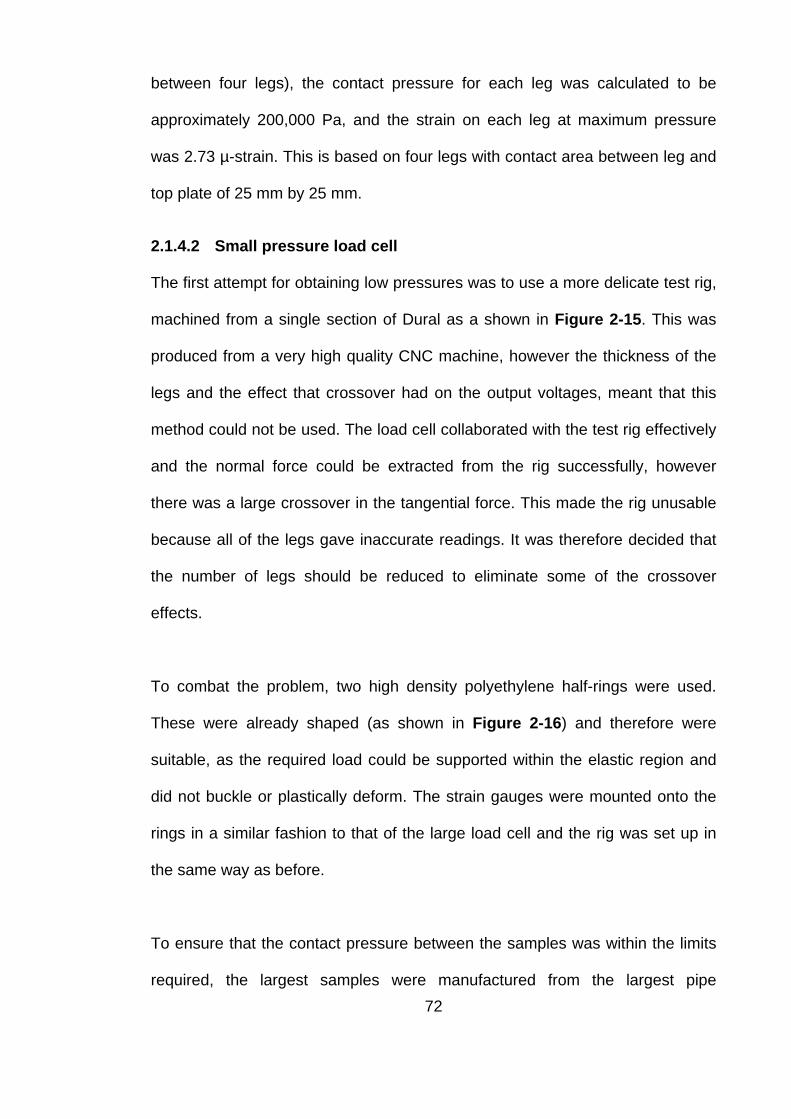
between four legs), the contact pressure for each leg was calculated to be
approximately 200,000 Pa, and the strain on each leg at maximum pressure
was 2.73 µ-strain. This is based on four legs with contact area between leg and
top plate of 25 mm by 25 mm.
2.1.4.2 Small pressure load cell
The first attempt for obtaining low pressures was to use a more delicate test rig,
machined from a single section of Dural as a shown in Figure 2-15. This was
produced from a very high quality CNC machine, however the thickness of the
legs and the effect that crossover had on the output voltages, meant that this
method could not be used. The load cell collaborated with the test rig effectively
and the normal force could be extracted from the rig successfully, however
there was a large crossover in the tangential force. This made the rig unusable
because all of the legs gave inaccurate readings. It was therefore decided that
the number of legs should be reduced to eliminate some of the crossover
effects.
To combat the problem, two high density polyethylene half-rings were used.
These were already shaped (as shown in Figure 2-16) and therefore were
suitable, as the required load could be supported within the elastic region and
did not buckle or plastically deform. The strain gauges were mounted onto the
rings in a similar fashion to that of the large load cell and the rig was set up in
the same way as before.
To ensure that the contact pressure between the samples was within the limits
required, the largest samples were manufactured from the largest pipe 72

available. In an ideal situation, the pipe size would preferably have been larger.
Nevertheless, the available pipe samples were deemed to be acceptable. To
achieve the contact pressure range between 20.68 MPa to 68.9 MPa (3 and 10
ksi), a force of 0.18 to 6.79 N was applied to the surface.
Figure 2-15: Regime 3 - attempt 2
Figure 2-16: Small pressure load cell
73

2.2 Calibration of load cell
Both the normal and tangential voltages had to be calibrated separately in order
to determine the forces they corresponded to. The normal force was calibrated
by measuring the normal and tangential voltage outputs when a known mass
was placed on top of the load cell (shown in Figure 2-17).
Figure 2-17: Load cell - normal force calibration set-up
If the legs of the load cell were perfectly symmetrical, applying a normal load
would produce only a normal voltage, and the tangential voltage would be zero
at the central position (a) on the top plate. However, even with the high
precision machinery used to manufacture them, the legs still harnessed
unavoidable imperfections. A very slight difference in one leg causes a
crossover between the normal and tangential forces, making it necessary that a
correctional calibration factor had to be determined.
74

To find the calibration equation for the system, masses were placed on different
positions of the load cell. If the legs had been identical, the tangential voltage
would be equal at positions b-d (left) and c-e (right) on the load cell (shown in
Figure 2-18). However as the two values were different, the discrepancy
needed to be taken into consideration. The normal voltages were measured for
a number of different masses, and this allowed a correctional factor to be
determined.
Figure 2-18: Load cell – top plate loading locations
On the top plate of the load cell, the masses were applied to the centre of the
face and the four corners. The weight (N) against the voltage (V) was plotted for
the three positions, as was the crossover for the system. As shown in Figure
2-19, the crossover increased as the weight was shifted from the right to the
left-hand side of the load cell.
75
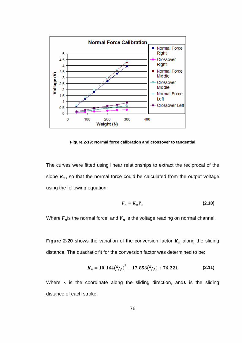
Figure 2-19: Normal force calibration and crossover to tangential
The curves were fitted using linear relationships to extract the reciprocal of the
slope 𝑲𝑲𝑻𝑻, so that the normal force could be calculated from the output voltage
using the following equation:
𝑭𝑭𝑻𝑻 = 𝑲𝑲𝑻𝑻𝑽𝑽𝑻𝑻 (2.10)
Where 𝑭𝑭𝑻𝑻is the normal force, and 𝑽𝑽𝑻𝑻 is the voltage reading on normal channel.
Figure 2-20 shows the variation of the conversion factor 𝑲𝑲𝑻𝑻 along the sliding
distance. The quadratic fit for the conversion factor was determined to be:
𝑲𝑲𝑻𝑻 = 𝟏𝟏𝟎𝟎.𝟏𝟏𝟏𝟏𝟒𝟒�𝒔𝒔 𝑳𝑳� �𝟐𝟐 − 𝟏𝟏𝟏𝟏.𝟖𝟖𝟖𝟖𝟏𝟏�𝒔𝒔 𝑳𝑳� � + 𝟏𝟏𝟏𝟏.𝟐𝟐𝟐𝟐𝟏𝟏 (2.11)
Where 𝒔𝒔 is the coordinate along the sliding direction, and𝑳𝑳 is the sliding
distance of each stroke.
76
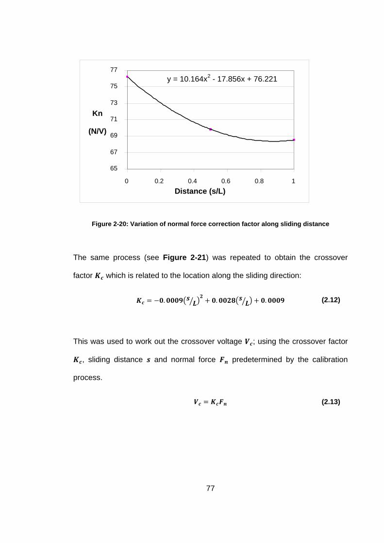
Figure 2-20: Variation of normal force correction factor along sliding distance
The same process (see Figure 2-21) was repeated to obtain the crossover
factor 𝑲𝑲𝑭𝑭 which is related to the location along the sliding direction:
𝑲𝑲𝑭𝑭 = −𝟎𝟎.𝟎𝟎𝟎𝟎𝟎𝟎𝟎𝟎�𝒔𝒔 𝑳𝑳� �𝟐𝟐 + 𝟎𝟎.𝟎𝟎𝟎𝟎𝟐𝟐𝟖𝟖�𝒔𝒔 𝑳𝑳� � + 𝟎𝟎.𝟎𝟎𝟎𝟎𝟎𝟎𝟎𝟎 (2.12)
This was used to work out the crossover voltage 𝑽𝑽𝑭𝑭; using the crossover factor
𝑲𝑲𝑭𝑭, sliding distance 𝒔𝒔 and normal force 𝑭𝑭𝑻𝑻 predetermined by the calibration
process.
𝑽𝑽𝑭𝑭 = 𝑲𝑲𝑭𝑭𝑭𝑭𝑻𝑻 (2.13)
y = 10.164x 2 - 17.856x + 76.221
65
67
69
71
73
75
77
0 0.2 0.4 0.6 0.8 1 Distance (s/L)
Kn
(N/V)
77

Figure 2-21: Crossover to tangential output voltage
These calibration factors were applied to the data obtained from testing,
providing a credible and reliable set of results.
To calibrate the tangential force, the setup shown in Figure 2-22 was used. The
load cell was held vertically so that the weight could be applied in the tangential
direction. This meant that the load applied was parallel to the top plate of the
load cell. This calibration process was similar to that of the normal component,
however in this case the masses were suspended from a rope attached to a
screw on the load cell. The mass was suspended from two locations on the top
plate to record the difference in the voltage reading, and therefore the effect of
positioning in the tangential direction. Similar to the normal voltage procedure,
when the tangential load was applied, a voltage in the tangential was registered.
y = -0.0009x 2 + 0.0028x + 0.0009
0.000
0.001
0.002
0.003
0.004
0 0.5 1 Distance (s/ L)
Kc
78

Figure 2-22: Schematic of tangential force calibration set-up
As shown in Figure 2-23, the slope of the linear range (up to 100 N) was 0.11
so that the reciprocal of the slope was 𝑲𝑲𝑻𝑻 = 𝟎𝟎.𝟎𝟎𝟖𝟖 (𝑵𝑵 𝑽𝑽)⁄ .Taking into account the
effect of crossover from normal force, the tangential force was derived using the
forumla:
𝑭𝑭𝑻𝑻 = 𝑲𝑲𝑻𝑻(𝑽𝑽𝑻𝑻 − 𝑽𝑽𝑭𝑭) (2.14)
Where 𝑽𝑽𝑻𝑻 is the voltage reading on the tangential force channel, and 𝑽𝑽𝑭𝑭 is the
crossover voltage from the normal force channel.
Suspended mass
Load cell
Load due to weight
79
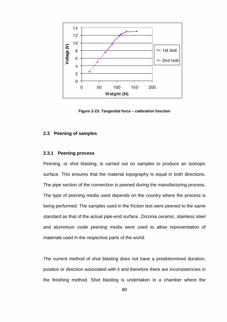
Figure 2-23: Tangential force – calibration function
2.3 Peening of samples
2.3.1 Peening process
Peening, or shot blasting, is carried out on samples to produce an isotropic
surface. This ensures that the material topography is equal in both directions.
The pipe section of the connection is peened during the manufacturing process.
The type of peening media used depends on the country where the process is
being performed. The samples used in the friction test were peened to the same
standard as that of the actual pipe-end surface. Zirconia ceramic, stainless steel
and aluminium oxide peening media were used to allow representation of
materials used in the respective parts of the world.
The current method of shot blasting does not have a predetermined duration,
position or direction associated with it and therefore there are inconsistencies in
the finishing method. Shot blasting is undertaken in a chamber where the
80
peening media is blasted at the surface using a moveable gun. The distance
from the gun’s position to the surface that is being treated is not defined, and
therefore it can be presumed that there are discrepancies between different
operators’ techniques. Slight changes in blasting angle or distance can alter the
way that the beads impact the surface. In the case of the ceramic peened
surface, a direct hit will produce a more isotropic pattern than that of an askew
one. Work by Higounenc (85) shows the complexity of the effect of the shot
peening characteristics on the final surface. There are various ways in which
the peening process can be undertaken and this can result in a number of
different features on the surfaces of the samples. It is therefore beneficial to
ensure that the peening process is standardised to ensure that all samples are
as similar as possible. This is difficult however because the angle of peening,
distance between gun and sample, blasting velocity of media and, most
importantly, the length of time that samples are peened for, all effect the surface
quality.
2.4 Lubrication in friction tests
During the make-up process, a lubricant is applied to the two surfaces in
contact. This is done with the intention to provide sufficient sliding between the
two surfaces, and to prevent galling from occurring. The lubricant used is
dependent upon the material type of the pin and coupling surfaces. A
comparison between three different lubricants was completed during the
project. The main lubricant (Lubricant A) under investigation is a proprietary
synthetic formula which was specifically designed to prevent galling of surfaces
during make-up. The other two lubricants are of industry standard. Lubricant B
81

contains large metal particles such as lead and nickel and the other, Lubricant
C, is an environmentally friendly substance which contains PTFE particles. It is
noted that Lubricant C did not stick well to the surfaces, and was easily
removed during testing.
Table 2-2: Properties of Lubricants
Properties Lubricant A Lubricant B Lubricant C
Base oil Lubricating Greases, Calcium Hydroxide Lubricating Greases
Petroleum distillates, Calcium
Compounds
Viscosity 50,000 cP (50 Pa.s) N/A N/A
Additives Non-metallic nano-particles
Metallic particles (Inc. graphite, lead, zinc,
copper)
Non-metallic particles (graphite)
Penetration N/A 310 – 340 300 – 340
Weight/ Gallon N/A 15.8 lbs/gallon 10.4 lbs/gallon
2.5 Testing Procedure
To provide a suitable representation of the two surfaces of the connection
during the make-up process, three cycles of the two samples sliding past one
another were completed. Due to the shape of the two surfaces being opposite
conically, there are limitations to where lubricant can become trapped in
comparison to the helical shape in the thread of the real connection. Therefore
the lubricant used in each experiment was reapplied between cycles to ensure
that the full effect of lubrication was felt for each section of the test.
82
Three different lubricants were used during testing; however the main results
were obtained using Lubricant A. This allowed a range of results to be attained
to provide a comparison for changes in make-up velocity, contact pressure,
surface roughness and peening media used to alter the surfaces.
Lubricant A was designed to be safer to use and more environmentally friendly.
Its primary function was galling resistance which, when combined with the
bronze plated chrome steel coupling, reduces the likelihood of defects on the
surface triggering leaks. The lubricant contains PTFE particles, has corrosion
protection properties, and also removes the need to clean the surfaces between
make-ups and break-outs.
Lubricant B and Lubricant C were both commercial industry lubricants.
Lubricant B was the most widely used but contained harmful particles including
lead and nickel. It was generally used with a copper plated chrome steel
coupling and a peened chrome steel pin-end pipe similar to the test set-up of
Lubricant A. The stiction properties of Lubricant B were relatively high and it
was not as easily removed from the surface compared to Lubricant C during
testing. Lubricant C was an environmentally friendly lubricant with similar
properties to Lubricant B, however did not contain harmful particles. There we
reissues with galling of surfaces for this lubricant however, and these detriments
were deemed to outweigh the benefits.
83
2.6 Repeatability
To ensure repeatability and comparability by using the same samples, the
design of the sample holders provided the possibility for rotation of the pins and
coupons in all three regimes. The design allowed three tests to be undertaken
on each sample. The data from each sample was compared and collaborated to
produce the final results. To ensure the tests were comparable, the two
surfaces in contact had to have the original surface topography. As illustrated in
Chapter 3, the initial stroke during the test removed the peaks from the surface.
This higher surface roughness value induced a slightly greater CoF compared
to that of the final cycles where the surface was smoother. This meant that it
was critical to ensure the surface roughness of all samples was comparable to
allow reliable data to be obtained.
84
Chapter 3 Surface Measurements
3.1 Measurement of roughness of surfaces
Topography defines the features of a surface. Appreciating topography of a
surface is fundamental in understanding tribology (86). It is also of significant
value in understanding the fatigue resistance (87). Surface roughness is one of
the most dominant characteristics which affects the friction and wear of a
system. As it affects the surface mechanics of a set-up so significantly,
measures have to be put in place to make sure it is controlled in manufacturing
processes. This ensures repeatability during testing and, most importantly,
maintains some kind of conformity in real-life situations where the value of CoF
is imperative to the success in operation.
An object’s surface roughness can be measured using various techniques,
including profilometers and various types of microscope. There are numerous
techniques available, and the technique deployed depends on the type of
surface, the quality of roughness measurement required and primarily, the
budget of the project. The most expensive methods can be extremely accurate
and useful, but the expense may outweigh the benefits. Measurement can be
done with or without contact between the device and the surface in question.
Rough surfaces are often considered to be unattractive due to the adverse
consequences of fatigue strength and wear resistance, as well as the
displeasing appearance that is produced (88).
85

3.1.1 Surface roughness measurement terms
The most common surface roughness values acquired during testing include
the arithmetic average roughness (𝑹𝑹𝒂𝒂) and the root mean square average
roughness �𝑹𝑹𝒒𝒒�. Other notable values are the Skewness (𝑹𝑹𝑺𝑺𝒌𝒌) and Kurtosis
(𝑹𝑹𝑲𝑲𝑫𝑫). The arithmetic average roughness is most commonly used to measure
the roughness of machined surfaces (89). It is informative for determining the
difference in the height profile of a surface. It is generally used to assess
manufacturing techniques. The arithmetic average surface roughness, also
known as the centre-line average (1), is calculated using simple statistical
formulae to calculate the average height of a set of data𝑦𝑦𝑖𝑖 .
𝑹𝑹𝒂𝒂 =𝟏𝟏𝑻𝑻�|𝒚𝒚𝑻𝑻|𝑻𝑻
𝑻𝑻=𝟏𝟏
(3.1)
The root mean squared average roughness represents the standard deviation
of the surface height. It is more useful for representing the optical finish of the
profile. It is essential in the calculation of the Skewness and Kurtosis. The
formula for calculating the r.m.s roughness value is:
𝑹𝑹𝒒𝒒 = �𝟏𝟏𝑻𝑻�(𝒚𝒚𝑻𝑻 − 𝒚𝒚)𝟐𝟐𝑻𝑻
𝑻𝑻=𝟏𝟏
(3.2)
The Skewness and Kurtosis values are related to the root mean square
roughness. The Skewness is calculated using the third root of the same
expression and Kurtosis is estimated using the fourth root (89). The Skewness
is an accurate definition of how symmetrical the data is about the central line
(90). Symmetrical data has a Skewness value close to zero. The value for
Skewness is used to determine how capable the surface is in carrying a load; it
also shows how porous the surface is, and is good for identifying the
86
characteristics of irregular machining processes. The value of skew can
become non-zero when the peaks of a rough surface are removed, if the
troughs of the surface are not altered at the same time (1). The Skew value can
be calculated using the following equation:
𝑹𝑹𝒔𝒔𝒌𝒌 = �𝟏𝟏
𝑻𝑻𝑹𝑹𝒒𝒒𝟑𝟑��𝒁𝒁𝑻𝑻 − 𝒁𝒁�
𝟑𝟑𝑻𝑻
𝑻𝑻=𝟏𝟏
𝟑𝟑
(3.3)
Kurtosis is defined as the "degree of peakedness of a distribution" (90); it
defines whether the height data is peaked or flat compared to the normal
distribution. Surfaces with normal or Gaussian distribution have a Kurtosis value
of 3 (91). The value depends upon both the peak and the tails of the distribution
of height data. Kurtosis is calculated using the equation:
𝑹𝑹𝒌𝒌𝑫𝑫 = �𝟏𝟏
𝑻𝑻𝑹𝑹𝒒𝒒𝟒𝟒��𝒁𝒁𝑻𝑻 − 𝒁𝒁�
𝟒𝟒𝑻𝑻
𝑻𝑻=𝟏𝟏
𝟒𝟒
(3.4)
3.2 Methods of measuring the surface roughness
3.2.1 Contact methods
Contact methods of measuring roughness include using a traditional stylus
profilometer and using an atomic force microscope (92). Both methods use a
stylus technique, where the nib of the stylus is drawn across the surface. In the
profilometer method, a very low force is applied and the surface roughness is
measured across one dimension, i.e. along a straight line of the surface. This
method is relatively inexpensive; however the main disadvantage is that,
particularly for soft materials, it can scratch the surface during testing thus
changing the roughness and surface properties. These are available both as
87

large set-ups and handheld devices; therefore the chosen type depends on the
requirements of the user. This method can be inaccurate due to the surface
area of the measurement being relatively small. Depending on the overall size
of the surface under investigation, the measurements it may not include all
features of the surface. This technique is much more suitable for surfaces with
isotropic structure and peaks and troughs of equal depth. The surface
roughness value will be significantly distorted and features on some sections of
the surface will not be accurately represented by the outcome value. To
improve accuracy, a high number of measurements need to be taken along the
surface. This can improve the precision of the result though it is very time
consuming, and costs can be relatively high.
The atomic force microscope is a variation on the Binnig and Rohrer invention
of the scanning tunnel microscope (STM) (93). The STM uses the technique of
scanning a sharp tip over a sample surface and measuring the force from the
deflection of springs. This is done by applying a voltage difference to the tip to
ensure that the surface and the device are close enough together. The theory is
based upon "tunnelling", a quantum mechanics effect where electrons that
characteristically should not have been able to move through a barrier, because
the electrons have insufficient energy in them, have been able to do so. In
quantum mechanics theory, electrons act as waves and therefore do not stop
suddenly but peter out quickly. If the obstacle is thin enough, some of these
electrons appear to be on the other side of the barrier. This phenomenon is
called tunnelling. In the case of the STM, the barrier is the air between the tip
and the sample. The current in the tip allows control of the distance between
88
sample and tip to be maintained (94). As the surface heights alter, the current
changes; the results of these are exhibited as an image. The output of the STM
produces a height matrix of the surface which can be used to calculate the
roughness of the material. The main issue with STM is that it can only be used
for metal substrates. Alterations to this technique were made to produce an
atomic force microscope (AFM) which could investigate any type of material.
The atomic force microscope (95) is a contact method which uses a similar
procedure to the STM, although instead of using a current to recognise peaks or
troughs it uses a probing tip. The tip is attached to a cantilever spring and the
angle between the two changes to trace the shape of the surface. The tip is
very fine and can react to microscopic features on the surface as it is designed
to respond to atomic forces (96). The device can then identify surface properties
and produce a set of measurements, including the roughness values in
nanometres.
3.2.2 Non-contact methods
Non-contact methods are becoming increasingly more favourable because this
technique removes the possibility of damaging a surface during measurement.
This technique uses optical sensors to measure the height of the asperities on a
surface. Three-dimensional images are created by stacking individual two-
dimensional layers on top of one another to create a replica surface. This is
executed by the device automatically and thus when reassembling the layers
together, the risk of human error is reduced. This type of measurement takes
longer than the contact types, however within one reading the entire area of the
89

surface is recorded. To do the same thing using a contact method would be far
more time-consuming, and the user of the device would have to locate the next
position of every line. By using only a two-dimensional device, there is a chance
that important sections of the surface could be missed out. The main
disadvantages of the three-dimensional method are the expense and
maintenance of the machine. Regular checks need to be done to maintain the
accuracy and the replacement of essential lenses, should they become
damaged, have large costs associated with them.
Laser scanning confocal and optical confocal microscopy are two of the most
common methods of non-contact profiling. They each have similar techniques,
however they use different light sources and receivers to create the image of
the surface and to store the data. The method used most commonly depends
on the accuracy required from the images, the types of samples being
investigated and, primarily, on the budget. Similar to other types of three-
dimensional microscopy, a confocal microscope recreates an image of the
surface point by point (97). The word confocal means "having a common focus
or foci" (98). It is where the device focuses on only one common point and
rejects the background 'noise' from outside the focal plane. To create the same
focus point, the pinhole only allows certain light beams through onto the
detector (shown in Figure 3-1). The laser confocal method (99) uses a laser
beam and a detector which has a pinhole in front of it. In contrast to a typical
microscope, where the device observes as far into a surface as it can; the
confocal microscope perceives an image one layer at a time. The depth of each
layer is determined by the user. The laser is shone onto a beam splitter, and
90

this light is shone onto a focal plane. The beam then projects back into the
direction of the pinhole and only light which is in focus is detected. This
detected light is then processed and an image of the required surface is
created. As the "image" is a matrix of surface heights, other useful values can
easily be obtained from it. This technique is useful for acquiring sharp images
with fine detail because there is no unfocussed light impairing the image quality.
Figure 3-1: Confocal laser microscope (97)
A Scanning Electron Microscopy (SEM) creates an image of the surface using
high-energy electrons. A beam of high-energy electrons are directed at the
sample and each type of material reacts to the electrons differently, giving off a
range of signals. It is these differences in electron reaction which allow the user
to establish which element types are present. This technique is used to gain
more information about the surface quality and structure (topography), chemical
make-up, and crystalline structure of the material. Although this method has
Pinhole
Beam-splitter
Focal
plane Laser
Detect
91
many advantages, the surface roughness cannot be measured using the
device. The accelerated electrons contain a considerable quantity of kinetic
energy and when these hit the sample they slow down, producing a number of
signals which can be picked up by the detector. Signal types include secondary
electrons, backscattered electrons, cathodoluminescence, auger electrons and
characteristic x-rays (100). During the SEM process (Figure 3-2), electrons are
blasted at the anode using an electron gun and these electrons pass through
the anode, directing them onto the magnetic lens. Current is applied to the
magnetic lens, creating a magnetic field. The electron beam passes through the
spinning coils and electron detector onto the sample. The beam can either pass
through the sample, missing all atoms within; collide with sample electrons to
create secondary electrons; or meet the nucleus of the sample atoms,
producing backscattered electrons. Each type of material produces a different
number of backscattered and secondary electrons, and the detector counts this
to identify the material type in the sample. It should also be noted that SEM
imaging is a non-destructive testing process, i.e. there is no reduction in sample
volume after testing; the testing process has to be undertaken in a vacuum.
3.3 Surface roughness measurement techniques
The value of CoF in a system depends highly on the characteristics of the
contacting surfaces. These contacting surfaces are dependent on the surface
roughness value, therefore it was important to ensure that this parameter was
kept constant during the tests. The roughness of each sample was measured to
ensure test consistency.
92
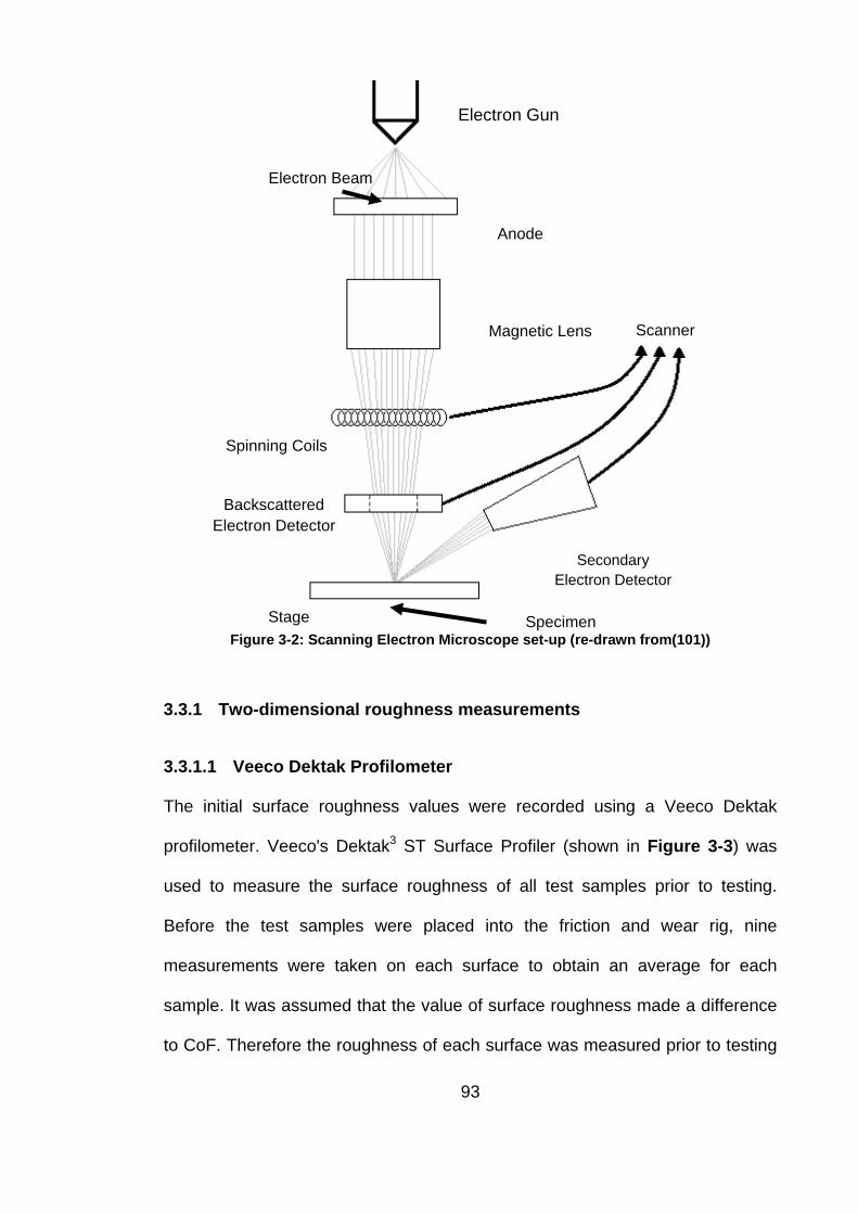
Figure 3-2: Scanning Electron Microscope set-up (re-drawn from(101))
3.3.1 Two-dimensional roughness measurements
3.3.1.1 Veeco Dektak Profilometer
The initial surface roughness values were recorded using a Veeco Dektak
profilometer. Veeco's Dektak3 ST Surface Profiler (shown in Figure 3-3) was
used to measure the surface roughness of all test samples prior to testing.
Before the test samples were placed into the friction and wear rig, nine
measurements were taken on each surface to obtain an average for each
sample. It was assumed that the value of surface roughness made a difference
to CoF. Therefore the roughness of each surface was measured prior to testing
Electron Gun
Anode
Magnetic Lens
Spinning Coils
Electron Beam
Backscattered Electron Detector
Specimen Stage
Secondary Electron Detector
Scanner
93
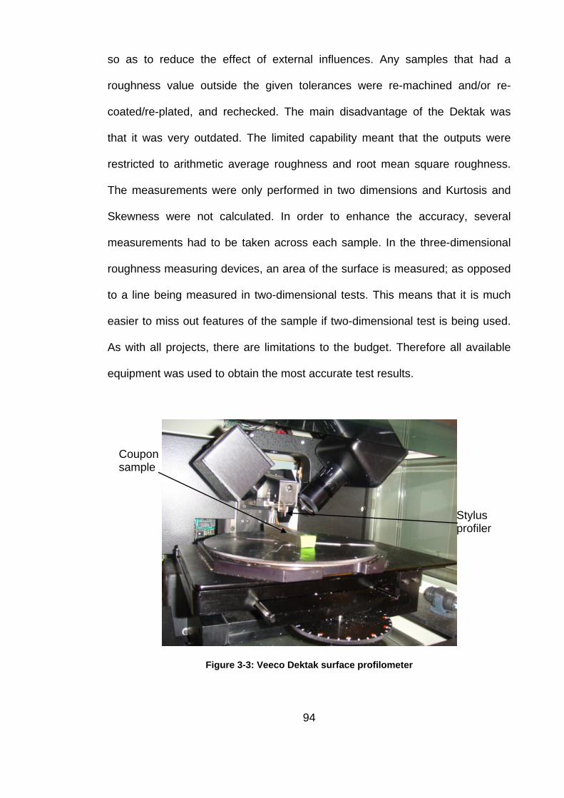
so as to reduce the effect of external influences. Any samples that had a
roughness value outside the given tolerances were re-machined and/or re-
coated/re-plated, and rechecked. The main disadvantage of the Dektak was
that it was very outdated. The limited capability meant that the outputs were
restricted to arithmetic average roughness and root mean square roughness.
The measurements were only performed in two dimensions and Kurtosis and
Skewness were not calculated. In order to enhance the accuracy, several
measurements had to be taken across each sample. In the three-dimensional
roughness measuring devices, an area of the surface is measured; as opposed
to a line being measured in two-dimensional tests. This means that it is much
easier to miss out features of the sample if two-dimensional test is being used.
As with all projects, there are limitations to the budget. Therefore all available
equipment was used to obtain the most accurate test results.
Figure 3-3: Veeco Dektak surface profilometer
Coupon sample
Stylus profiler
94
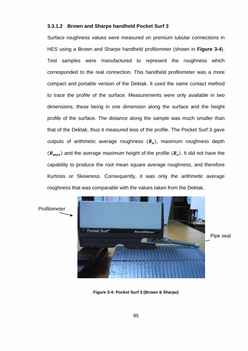
3.3.1.2 Brown and Sharpe handheld Pocket Surf 3
Surface roughness values were measured on premium tubular connections in
HES using a Brown and Sharpe handheld profilometer (shown in Figure 3-4).
Test samples were manufactured to represent the roughness which
corresponded to the real connection. This handheld profilometer was a more
compact and portable version of the Dektak. It used the same contact method
to trace the profile of the surface. Measurements were only available in two
dimensions, these being in one dimension along the surface and the height
profile of the surface. The distance along the sample was much smaller than
that of the Dektak, thus it measured less of the profile. The Pocket Surf 3 gave
outputs of arithmetic average roughness (𝑹𝑹𝒂𝒂), maximum roughness depth
(𝑹𝑹𝒎𝒎𝒂𝒂𝒙𝒙) and the average maximum height of the profile (𝑹𝑹𝒛𝒛). It did not have the
capability to produce the root mean square average roughness, and therefore
Kurtosis or Skewness. Consequently, it was only the arithmetic average
roughness that was comparable with the values taken from the Dektak.
Figure 3-4: Pocket Surf 3 (Brown & Sharpe)
Pipe seal
Profilometer
95

3.3.2 Three-dimensional roughness measurements
For that reason, a more accurate three-dimensional profile of the surface
topography needed to be made. This was initially done using the Zygo
Interferometer (OMP-0347K shown in Figure 3-5) in the University of
Cambridge, and more recently using the Olympus LEXT Laser Confocal
Microscope in Plymouth University.
Optical interferometry is the study of measuring distances using the interference
of light waves. Interferometers are very precise, accurate machines which use a
light source and mirrors to create an image of the surface profile. The output is
a measure of the interference. A beam is split into two halves and an optical
light is directed at a piece of glass coated with silver (known as the beam-
splitter); half of the light passes through and half reflects back. The silver coated
glass material acts as a cross between a mirror and a piece of glass. One beam
shines onto a mirror and then onto a screen or camera and the other beam
shines on or through the surface being measured then onto a second mirror and
back through the beam splitter, and finally back to the same screen or camera.
Due to the shifting distance and direction that the second beam travels to the
first beam, it becomes out of phase with the first beam. The two beams meet up
on the screen or camera and here they interfere with one another. Dark and
light areas are produced from the phase difference between the images. Light
areas are created at sections where the two beams have been added together
(which is defined as constructive interference) and dark areas are created
where the beams have been subtracted from each other (destructive
96

interference). The pattern produced from the interference data provides the
information that can be accurately measured. One disadvantage of the
interferometer is that it gives the best results and images when the material is
shiny. Duller materials, particularly the manganese phosphate bathed carbon
used in some of the tests, do not generate as good an image when compared to
other surfaces.
Figure 3-5: Zygo Interferometer (OMP-0347K)
3.4 Peening media and sample images
The word "peen" is of Scandinavian origin, it comes from the Danish "pene"
which means to beat (out) (98). Processes such as shot blasting (or peening)
are generally used for opposing crack formation and growth, by inducing a
compressive residual stress layer around the surface of a material (1) i.e.
stresses within the structure which are not subjected to the external
Sample
Light source and receiver
97

compressive forces. Small particles of a chosen material are propelled onto a
surface through a gun using air pressure. Peening plastically deforms the
surface of the material alleviating it from some of the localised stresses
associated with the situation in which it is placed in (102). A peening technique
was used to refine the surface of the pipe section of the connection. This
peening practice produces an even surface, removing the machining lines and
leaving an isotropic surface. As the connection pieces are relatively thick, it is
only the surface which deforms during the peening process, and therefore it
does not lose its shape.
3.4.1 Peening media
Since local materials are used to peen surfaces, different materials are utilised
in various parts of the world. An assortment of materials was used for shot
peening, including ceramic and metal particles. The peening media was
examined under a microscope to observe the differences between the size and
shape of the particles. Finer stainless steel peening media (Figure 3-6),
ceramic (Figure 3-7) and coarser stainless steel (Figure 3-8) media types were
available for inspection.
98

Figure 3-6: ≤0.2mm stainless steel peening media
Figure 3-7: Ceramic peening media
Figure 3-8: Coarser stainless steel peening media
99

The shape and size of the individual peening medium can be seen in the above
images. The ceramic media is of spherical character compared to the coarse
and fine stainless steel. The ceramic material is made from a composition of
Zirconium Oxide (𝒁𝒁𝑭𝑭𝑶𝑶𝟐𝟐), Silicon Oxide (𝑺𝑺𝑻𝑻𝑶𝑶𝟐𝟐) and Aluminium Oxide (𝑨𝑨𝑻𝑻𝟐𝟐𝑶𝑶𝟑𝟑)
particles. The general make-up of the composition is approximately 60-70wt%
𝒁𝒁𝑭𝑭𝑶𝑶𝟐𝟐, 28-33wt% 𝑺𝑺𝑻𝑻𝑶𝑶𝟐𝟐 and less than 10wt% 𝑨𝑨𝑻𝑻𝟐𝟐𝑶𝑶𝟑𝟑 (103). The composition of
the finer stainless steel particles is approximately 30wt% Chromium (Cr), up to
2wt% Silicon (Si), up to 2wt% Manganese (Mn), up to 3wt% Carbon (C) and up
to 4wt% Molybdenum (Mo), leaving the remaining 59wt% of material to be Iron
(Fe). The finer stainless steel particles are the smallest size available of this
material (the particle sizes are below 0.14 mm in size) and are designed to
improve the quality of the surface finish and reduce the blasting time.
To shot peen a material, a set of media is blasted at a surface using a high
pressure air gun. The shot peening media size, structure and shape plays a
huge part in the surface structure of the final product, as does the distance and
direction that peening is done. The ceramic media is spherical in shape and its
composition has very few sharp edges or corners. This results in the majority of
troughs being circular.
The stainless steel media is larger in size to that of the ceramic material. This
resulted in larger craters on its surface. The stainless steel peening media was
quite sharp and contained various different sizes of particles. The profile of the
peened surface therefore had a wide range of different sizes of troughs.
100

3.4.2 Surface roughness of peened samples
Table 3-1 shows the equivalent arithmetic average surface roughness (Ra)
values for the pin (shown in Figure 3-9 (a)) and coupon (shown in Figure 3-9
(b)) samples, manufactured for testing for ceramic peened, coarse stainless
steel peened, aluminium oxide peened and finer stainless steepened tests.
Figure 3-9: Geometry of the samples for used in tests (a) Pin (b) Coupon
Table 3-1: Peening media and roughness of coupon or pin
Surface Peening Coupon Pin
Ra (μm) Ra (μinch) Ra (μm) Ra (μinch)
Ceramic 1.60±0.23 65.17±5.97 1.52±0.12 62.18±4.72
Coarser Stainless
steel 1.18±0.19 48.16±7.49 0.81±0.11 33.06±4.33
Aluminium Oxide 2.88±0.34 117.59±13.39 2.45±0.22 99.92±8.66
Finer Stainless
Steel 0.92±0.11 37.48± 4.33 1.15±0.31 46.94±12.21
The stainless steel peened coupons and pins had a lower arithmetic average
surface roughness than those measured on the premium tubular connection.
The procedure for peening was supposed to be similar to that of the process
used in everyday manufacture. Microscopic images of the surfaces showed the
(a) (b)
101
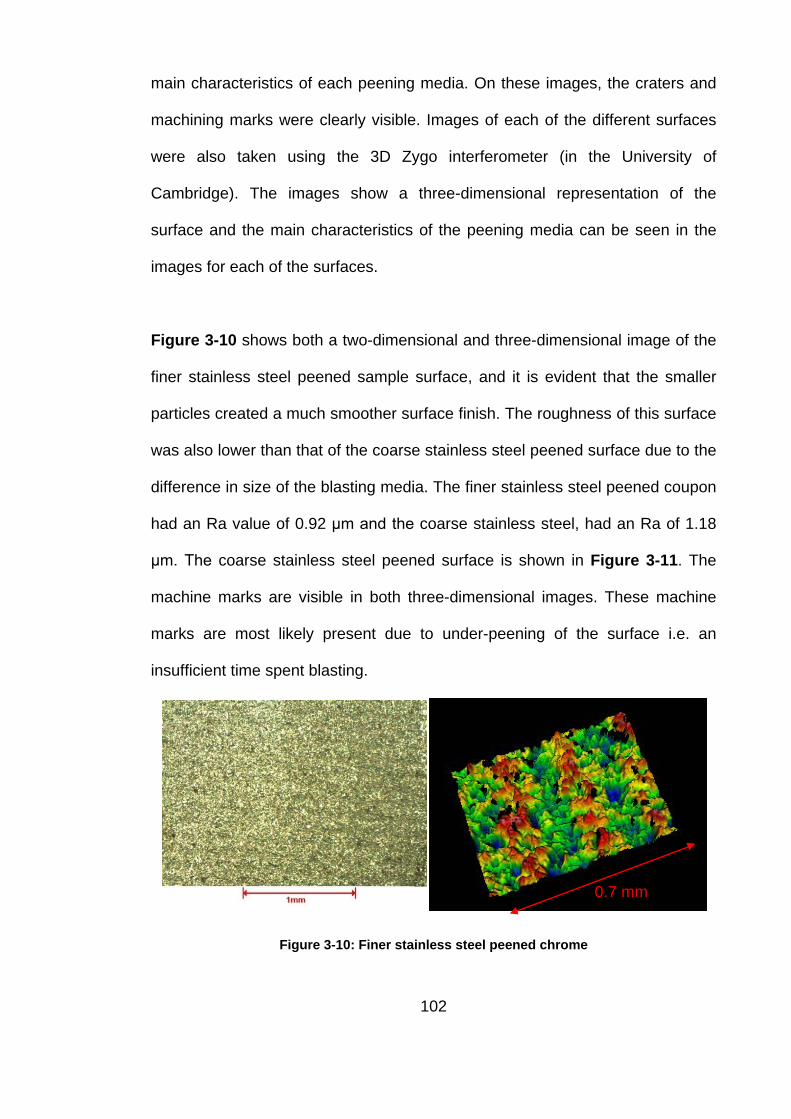
main characteristics of each peening media. On these images, the craters and
machining marks were clearly visible. Images of each of the different surfaces
were also taken using the 3D Zygo interferometer (in the University of
Cambridge). The images show a three-dimensional representation of the
surface and the main characteristics of the peening media can be seen in the
images for each of the surfaces.
Figure 3-10 shows both a two-dimensional and three-dimensional image of the
finer stainless steel peened sample surface, and it is evident that the smaller
particles created a much smoother surface finish. The roughness of this surface
was also lower than that of the coarse stainless steel peened surface due to the
difference in size of the blasting media. The finer stainless steel peened coupon
had an Ra value of 0.92 μm and the coarse stainless steel, had an Ra of 1.18
μm. The coarse stainless steel peened surface is shown in Figure 3-11. The
machine marks are visible in both three-dimensional images. These machine
marks are most likely present due to under-peening of the surface i.e. an
insufficient time spent blasting.
Figure 3-10: Finer stainless steel peened chrome
0.7 mm
102
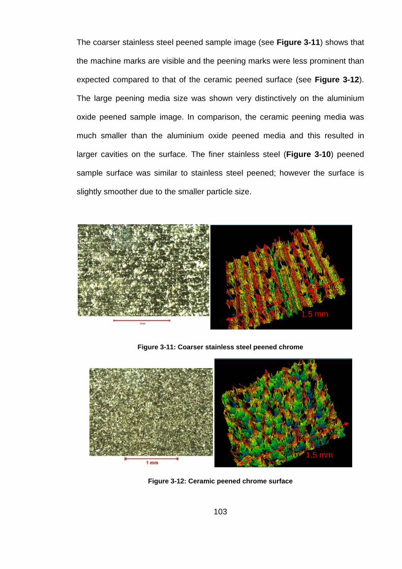
The coarser stainless steel peened sample image (see Figure 3-11) shows that
the machine marks are visible and the peening marks were less prominent than
expected compared to that of the ceramic peened surface (see Figure 3-12).
The large peening media size was shown very distinctively on the aluminium
oxide peened sample image. In comparison, the ceramic peening media was
much smaller than the aluminium oxide peened media and this resulted in
larger cavities on the surface. The finer stainless steel (Figure 3-10) peened
sample surface was similar to stainless steel peened; however the surface is
slightly smoother due to the smaller particle size.
Figure 3-11: Coarser stainless steel peened chrome
Figure 3-12: Ceramic peened chrome surface
1.5 mm
1.5 mm
103
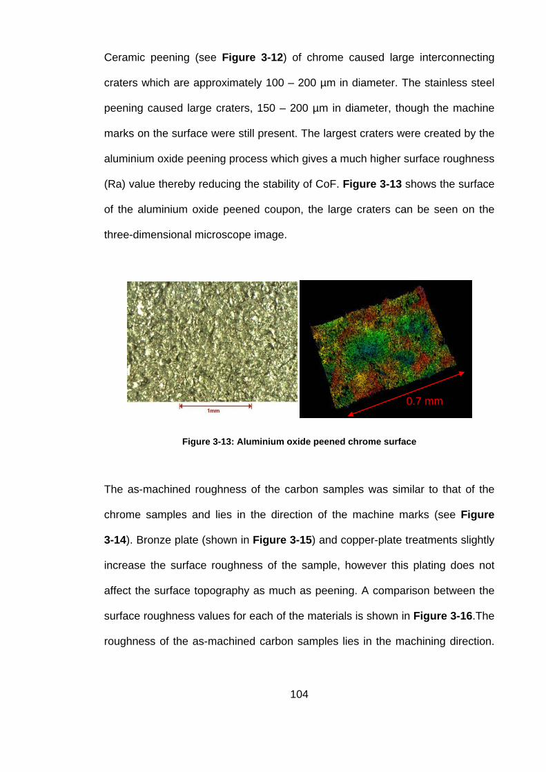
Ceramic peening (see Figure 3-12) of chrome caused large interconnecting
craters which are approximately 100 – 200 µm in diameter. The stainless steel
peening caused large craters, 150 – 200 µm in diameter, though the machine
marks on the surface were still present. The largest craters were created by the
aluminium oxide peening process which gives a much higher surface roughness
(Ra) value thereby reducing the stability of CoF. Figure 3-13 shows the surface
of the aluminium oxide peened coupon, the large craters can be seen on the
three-dimensional microscope image.
Figure 3-13: Aluminium oxide peened chrome surface
The as-machined roughness of the carbon samples was similar to that of the
chrome samples and lies in the direction of the machine marks (see Figure
3-14). Bronze plate (shown in Figure 3-15) and copper-plate treatments slightly
increase the surface roughness of the sample, however this plating does not
affect the surface topography as much as peening. A comparison between the
surface roughness values for each of the materials is shown in Figure 3-16.The
roughness of the as-machined carbon samples lies in the machining direction.
0.7 mm
104
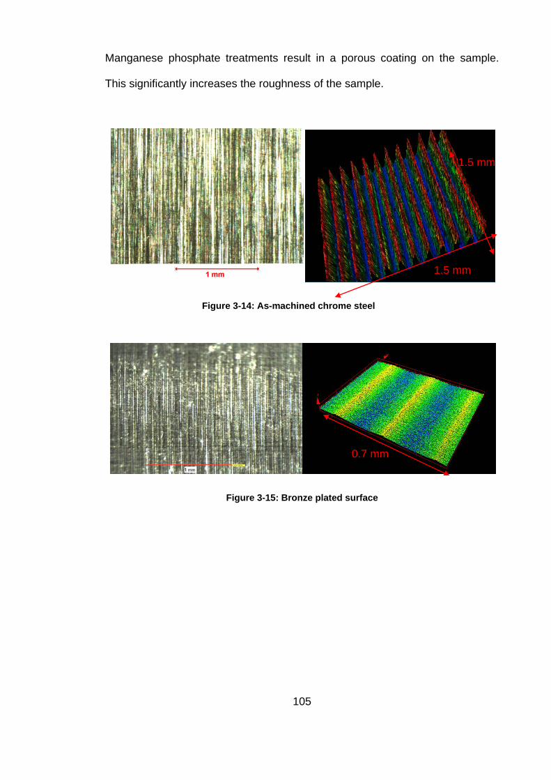
Manganese phosphate treatments result in a porous coating on the sample.
This significantly increases the roughness of the sample.
Figure 3-14: As-machined chrome steel
Figure 3-15: Bronze plated surface
1.5 mm
0.7 mm
1.5 mm
105
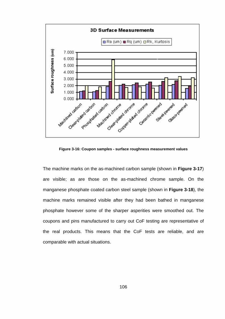
Figure 3-16: Coupon samples - surface roughness measurement values
The machine marks on the as-machined carbon sample (shown in Figure 3-17)
are visible; as are those on the as-machined chrome sample. On the
manganese phosphate coated carbon steel sample (shown in Figure 3-18), the
machine marks remained visible after they had been bathed in manganese
phosphate however some of the sharper asperities were smoothed out. The
coupons and pins manufactured to carry out CoF testing are representative of
the real products. This means that the CoF tests are reliable, and are
comparable with actual situations.
106
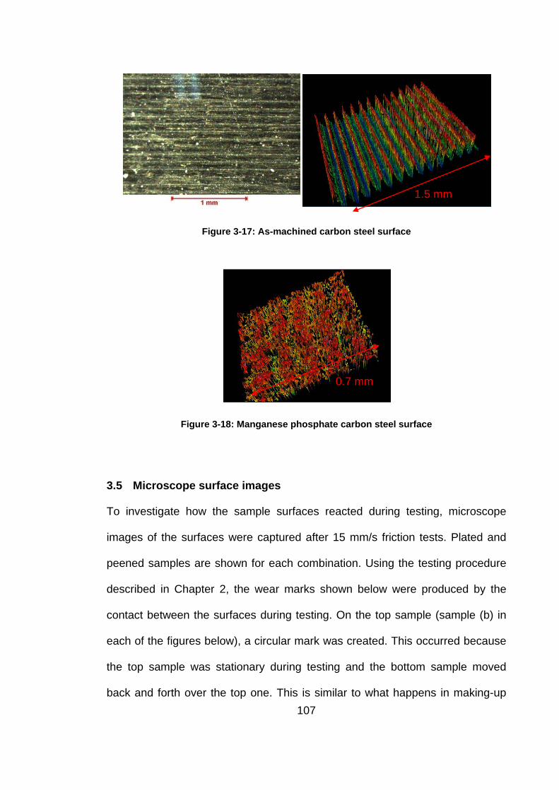
Figure 3-17: As-machined carbon steel surface
Figure 3-18: Manganese phosphate carbon steel surface
3.5 Microscope surface images
To investigate how the sample surfaces reacted during testing, microscope
images of the surfaces were captured after 15 mm/s friction tests. Plated and
peened samples are shown for each combination. Using the testing procedure
described in Chapter 2, the wear marks shown below were produced by the
contact between the surfaces during testing. On the top sample (sample (b) in
each of the figures below), a circular mark was created. This occurred because
the top sample was stationary during testing and the bottom sample moved
back and forth over the top one. This is similar to what happens in making-up
1.5 mm
0.7 mm
107

the premium tubular connection. The bottom sample (sample (a) in each of the
figures) experienced a linear wear mark along the 45 mm length of contact. The
directions of travel are identified on the samples below by the arrows. On the
peened samples, the machining marks which were a result of the manufacturing
procedure are visible; this shows that the peening process only changes the
surface topography but the structure of the material is intact.
3.5.1 Visual outcome of the bronze plated and peened samples after
testing
3.5.1.1 Bronze plated – ceramic peened wear marks
Figure 3-19 shows the bronze plate and ceramic peened surfaces after the 15
mm/s friction test. The left hand (L) image shows the wear mark on the bronze
plate surface. This wear mark is less prevalent compared to the mark on the
surface during the stainless steel test. However it did not scratch the surface as
much as during the stainless steel investigation (shown in Figure 3-19). In both
peened samples, it is evident that machining marks on the plated samples
made a difference to the wear on the peened surface. The peened surface in
each case has a set of scratch marks along the sliding direction. These are
caused by a combination of the peaks of machine marks on the plated surface
and debris from the top surface being removed, leaving the deepest pits on the
peened surface. This indicates that there is significant wear on the peened
surface in both cases.
108

Figure 3-19: Surface images after test (L) Bronze plate and (R) ceramic peened chrome
steel
3.5.1.2 Bronze plated – stainless steel peened wear marks
Figure 3-20: Surface images after test (L) bronze plated (R) stainless steel peened chrome steel bronze plated – aluminium oxide peened wear marks
The wear marks on the bronze plate surface for the aluminium oxide test
(shown in Figure 3-21) are much more prevalent than on the ceramic or
stainless steel tests. This is due to the higher roughness of the aluminium oxide
peened surface. The wear marks on the peened surface are relatively deep
compared to the other tests and the removal and build-up of material is
apparent.
1 mm 1 mm
1 mm 1 mm
109
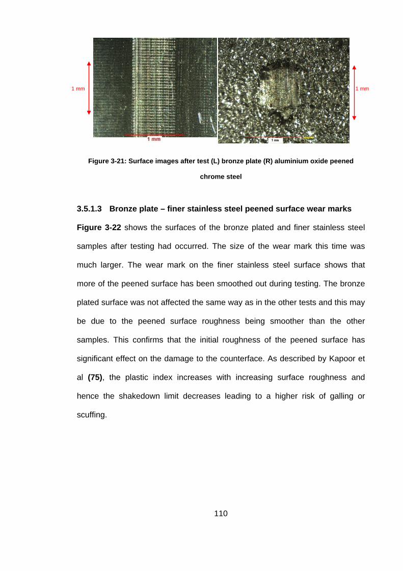
Figure 3-21: Surface images after test (L) bronze plate (R) aluminium oxide peened
chrome steel
3.5.1.3 Bronze plate – finer stainless steel peened surface wear marks
Figure 3-22 shows the surfaces of the bronze plated and finer stainless steel
samples after testing had occurred. The size of the wear mark this time was
much larger. The wear mark on the finer stainless steel surface shows that
more of the peened surface has been smoothed out during testing. The bronze
plated surface was not affected the same way as in the other tests and this may
be due to the peened surface roughness being smoother than the other
samples. This confirms that the initial roughness of the peened surface has
significant effect on the damage to the counterface. As described by Kapoor et
al (75), the plastic index increases with increasing surface roughness and
hence the shakedown limit decreases leading to a higher risk of galling or
scuffing.
1 mm 1 mm
110

Figure 3-22: Surface images after test (L) bronze plate (R) finer stainless steel peened
chrome steel
3.6 SEM imaging and composition analysis
SEM imaging was undertaken to improve the understanding of the surface
structure. Figure 3-23 shows the surface of the ceramic peened sample. The
main structure of the surface is visible and the location of the ceramic peened
holes can be clearly observed. The asperities created through peening are
visible on the surface and these seem to be uniformly distributed. The width of
the sample is approximately 2.5 mm.
Figure 3-24 shows an image with higher magnification of the surface structure.
Where the surface has been blasted with the ceramic particles, there is a pile-
up of material around the crater. There are various sizes of craters on the
surface, some of which are spherical. The size of the craters depends on both
the size of the peening media and the force with which they were blasted at the
surface.
1 mm 1 mm
111
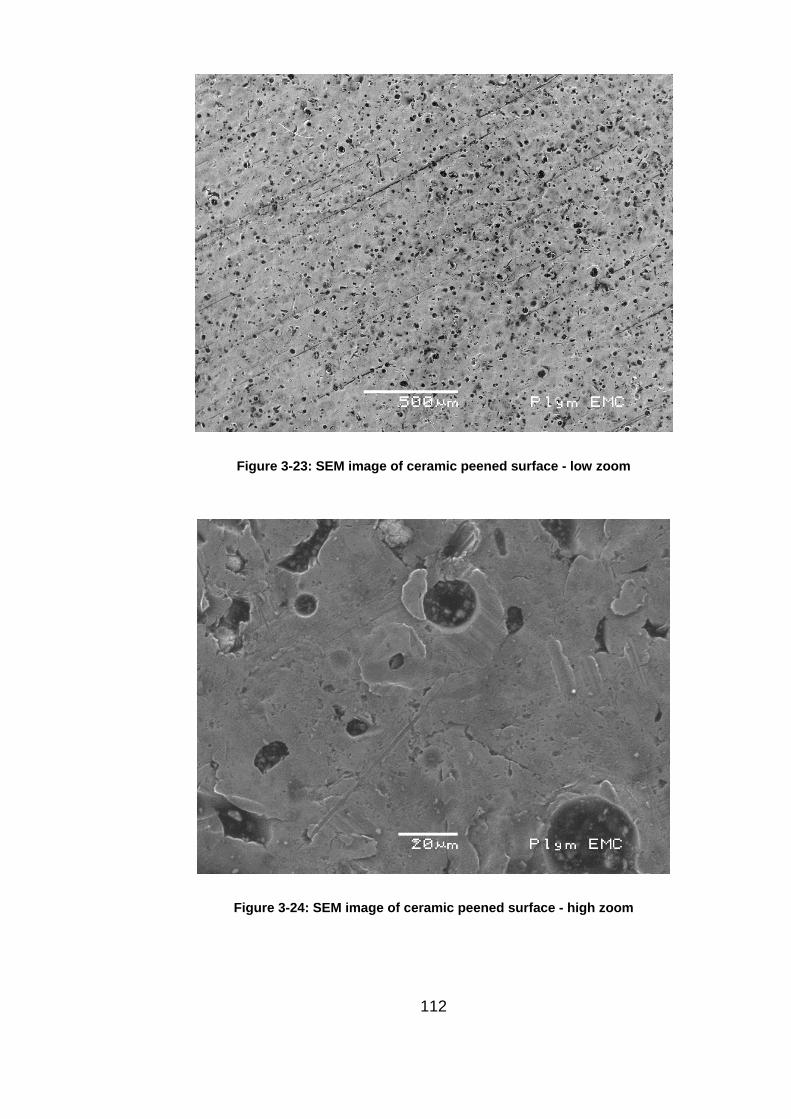
Figure 3-23: SEM image of ceramic peened surface - low zoom
Figure 3-24: SEM image of ceramic peened surface - high zoom
112
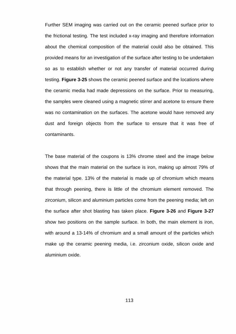
Further SEM imaging was carried out on the ceramic peened surface prior to
the frictional testing. The test included x-ray imaging and therefore information
about the chemical composition of the material could also be obtained. This
provided means for an investigation of the surface after testing to be undertaken
so as to establish whether or not any transfer of material occurred during
testing. Figure 3-25 shows the ceramic peened surface and the locations where
the ceramic media had made depressions on the surface. Prior to measuring,
the samples were cleaned using a magnetic stirrer and acetone to ensure there
was no contamination on the surfaces. The acetone would have removed any
dust and foreign objects from the surface to ensure that it was free of
contaminants.
The base material of the coupons is 13% chrome steel and the image below
shows that the main material on the surface is iron, making up almost 79% of
the material type. 13% of the material is made up of chromium which means
that through peening, there is little of the chromium element removed. The
zirconium, silicon and aluminium particles come from the peening media; left on
the surface after shot blasting has taken place. Figure 3-26 and Figure 3-27
show two positions on the sample surface. In both, the main element is iron,
with around a 13-14% of chromium and a small amount of the particles which
make up the ceramic peening media, i.e. zirconium oxide, silicon oxide and
aluminium oxide.
113

Figure 3-25: X-ray SEM Image of ceramic peened surface prior to friction testing
Figure 3-26: Chemical composition of ceramic peened surface prior to friction testing -
Specimen 4
Specimen 17
Specimen 4
114
Figure 3-27: Chemical composition of ceramic peened surface prior to friction testing -
Specimen 17
Figure 3-26 shows the corresponding graphs from the SEM image of the
bronze plate (Figure 3-25). This shows the chemical composition of the bronze
plate surface. Bronze plate is a 50% tin and 50% copper composition.
After the friction test was performed at 15 mm/s, SEM images were retaken on
the surface. Similar to the measurements for the samples before testing, the
surfaces were cleaned in acetone using a magnetic stirrer. The surfaces were
not "wiped" after testing so any transfer should have been visible using the
SEM. Removing the lubricant by wiping would have altered the surface and any
transferred material would have been most likely removed. Nevertheless, there
is a degree of uncertainty in using the acetone cleaner and ultrasonic bath;
however without cleaning the surface, the main constituents of the
115

measurement would have been the lubricant. The SEM does not possess the
capability to investigate liquids.
Figure 3-28: X-ray SEM Image of Bronze plate surface prior to testing
Figure 3-29: Chemical composition of bronze plated surface prior to testing
Spectrum 135
116
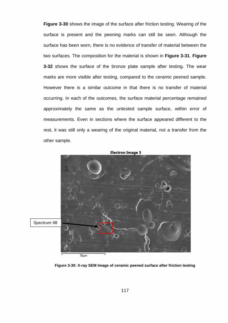
Figure 3-30 shows the image of the surface after friction testing. Wearing of the
surface is present and the peening marks can still be seen. Although the
surface has been worn, there is no evidence of transfer of material between the
two surfaces. The composition for the material is shown in Figure 3-31. Figure
3-32 shows the surface of the bronze plate sample after testing. The wear
marks are more visible after testing, compared to the ceramic peened sample.
However there is a similar outcome in that there is no transfer of material
occurring. In each of the outcomes, the surface material percentage remained
approximately the same as the untested sample surface, within error of
measurements. Even in sections where the surface appeared different to the
rest, it was still only a wearing of the original material, not a transfer from the
other sample.
Figure 3-30: X-ray SEM Image of ceramic peened surface after friction testing
Spectrum 98
117
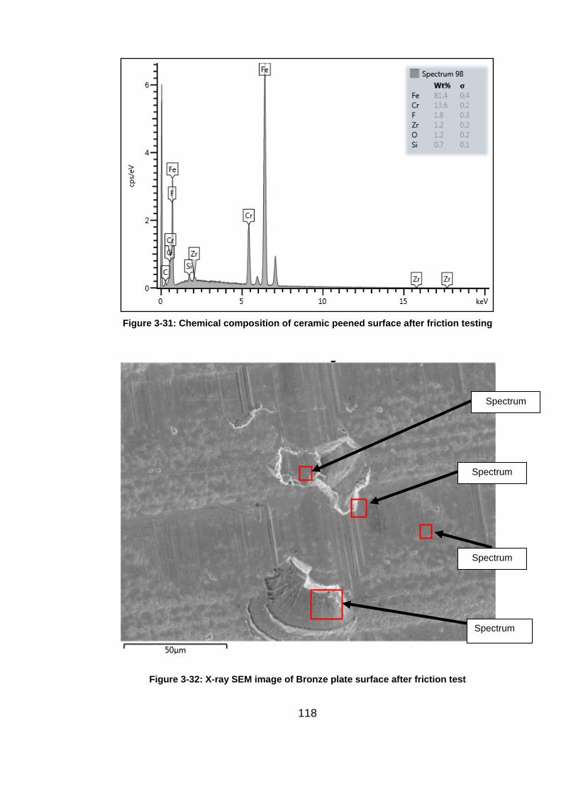
Figure 3-31: Chemical composition of ceramic peened surface after friction testing
Figure 3-32: X-ray SEM image of Bronze plate surface after friction test
Spectrum
Spectrum
Spectrum
Spectrum
118
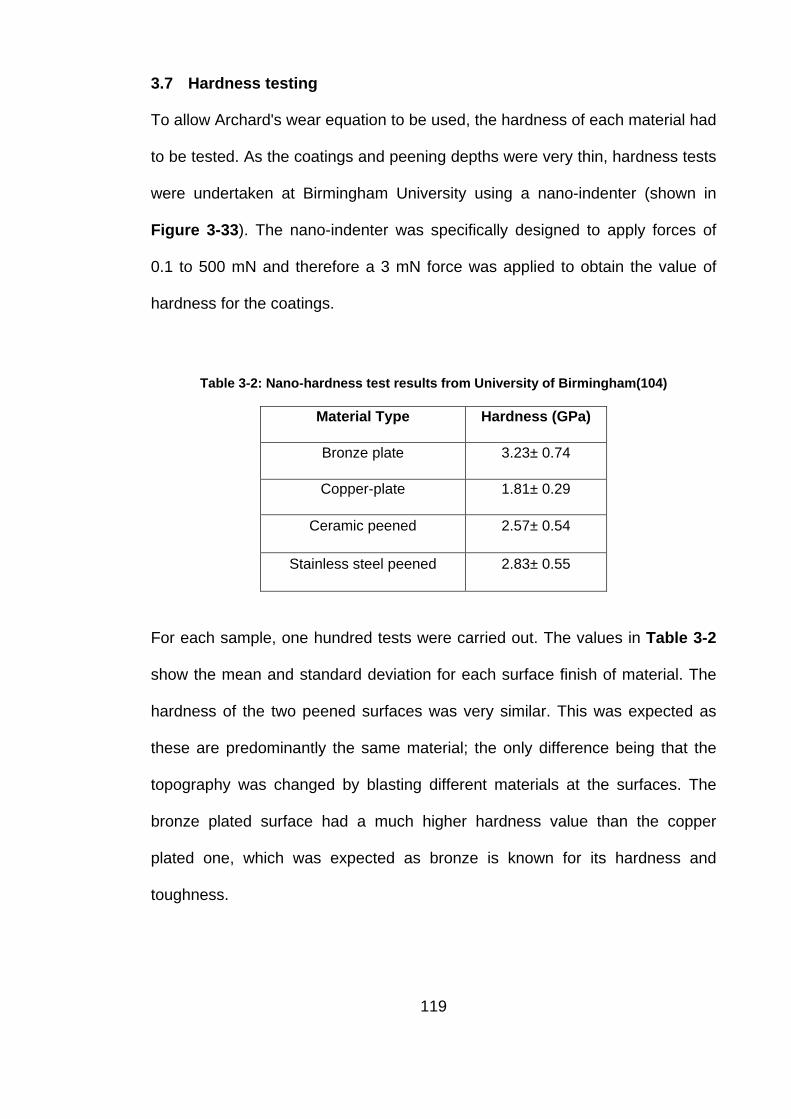
3.7 Hardness testing
To allow Archard's wear equation to be used, the hardness of each material had
to be tested. As the coatings and peening depths were very thin, hardness tests
were undertaken at Birmingham University using a nano-indenter (shown in
Figure 3-33). The nano-indenter was specifically designed to apply forces of
0.1 to 500 mN and therefore a 3 mN force was applied to obtain the value of
hardness for the coatings.
Table 3-2: Nano-hardness test results from University of Birmingham(104)
Material Type Hardness (GPa)
Bronze plate 3.23± 0.74
Copper-plate 1.81± 0.29
Ceramic peened 2.57± 0.54
Stainless steel peened 2.83± 0.55
For each sample, one hundred tests were carried out. The values in Table 3-2
show the mean and standard deviation for each surface finish of material. The
hardness of the two peened surfaces was very similar. This was expected as
these are predominantly the same material; the only difference being that the
topography was changed by blasting different materials at the surfaces. The
bronze plated surface had a much higher hardness value than the copper
plated one, which was expected as bronze is known for its hardness and
toughness.
119

Figure 3-33: MicroMaterialsnano-testnano-indenter
120

Chapter 4 : Surface Topography Evolution and
Coefficient of Friction
4.1 Test regimes
The intention of this research is to provide conclusions that can expose the
general trend of how CoF is affected by changes in external circumstances
during make-up of a premium tubular connection, in an oil and gas well. The
main areas of concern were in the differences of CoF during sliding (or in this
case, make-up of the connections) caused by changes in contact pressure,
sliding speed, material properties, surface roughness values and lubrication.
Changes in CoF had the potential to cause a problem because torque is
calculated using the CoF value. To understand how each external circumstance
affected the results, a set of combinations was pre-defined with the support of
engineers from the manufacturer.
Using knowledge and results from previous laboratory tests, the list was
developed to include the major circumstantial changes. It was known
theoretically, according to Coulomb (34) and proven through an extensive
number of experiments by Morin (3) that CoF did not change with varying
sliding speeds. However, there is evidence to prove that this might not be
entirely true and that this was primarily a fact in dry sliding conditions only. Work
by Al-Samari et al (105) showed that CoF reduced with increasing sliding
velocity. The authors’ work also investigated the effect of surface roughness,
normal force and relative humidity. Although the results were obtained using a
pin-on-disc tribo-tester, there is uncertainty in the accuracy of the results. It was
121
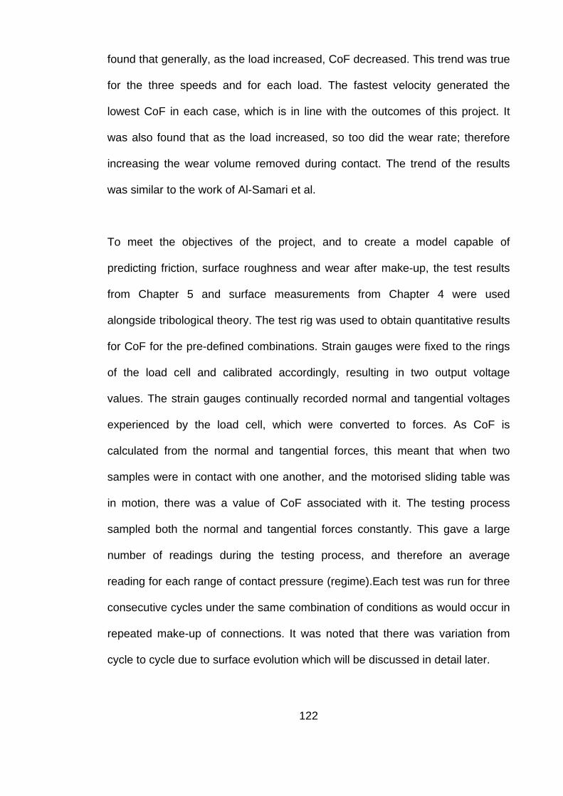
found that generally, as the load increased, CoF decreased. This trend was true
for the three speeds and for each load. The fastest velocity generated the
lowest CoF in each case, which is in line with the outcomes of this project. It
was also found that as the load increased, so too did the wear rate; therefore
increasing the wear volume removed during contact. The trend of the results
was similar to the work of Al-Samari et al.
To meet the objectives of the project, and to create a model capable of
predicting friction, surface roughness and wear after make-up, the test results
from Chapter 5 and surface measurements from Chapter 4 were used
alongside tribological theory. The test rig was used to obtain quantitative results
for CoF for the pre-defined combinations. Strain gauges were fixed to the rings
of the load cell and calibrated accordingly, resulting in two output voltage
values. The strain gauges continually recorded normal and tangential voltages
experienced by the load cell, which were converted to forces. As CoF is
calculated from the normal and tangential forces, this meant that when two
samples were in contact with one another, and the motorised sliding table was
in motion, there was a value of CoF associated with it. The testing process
sampled both the normal and tangential forces constantly. This gave a large
number of readings during the testing process, and therefore an average
reading for each range of contact pressure (regime).Each test was run for three
consecutive cycles under the same combination of conditions as would occur in
repeated make-up of connections. It was noted that there was variation from
cycle to cycle due to surface evolution which will be discussed in detail later.
122
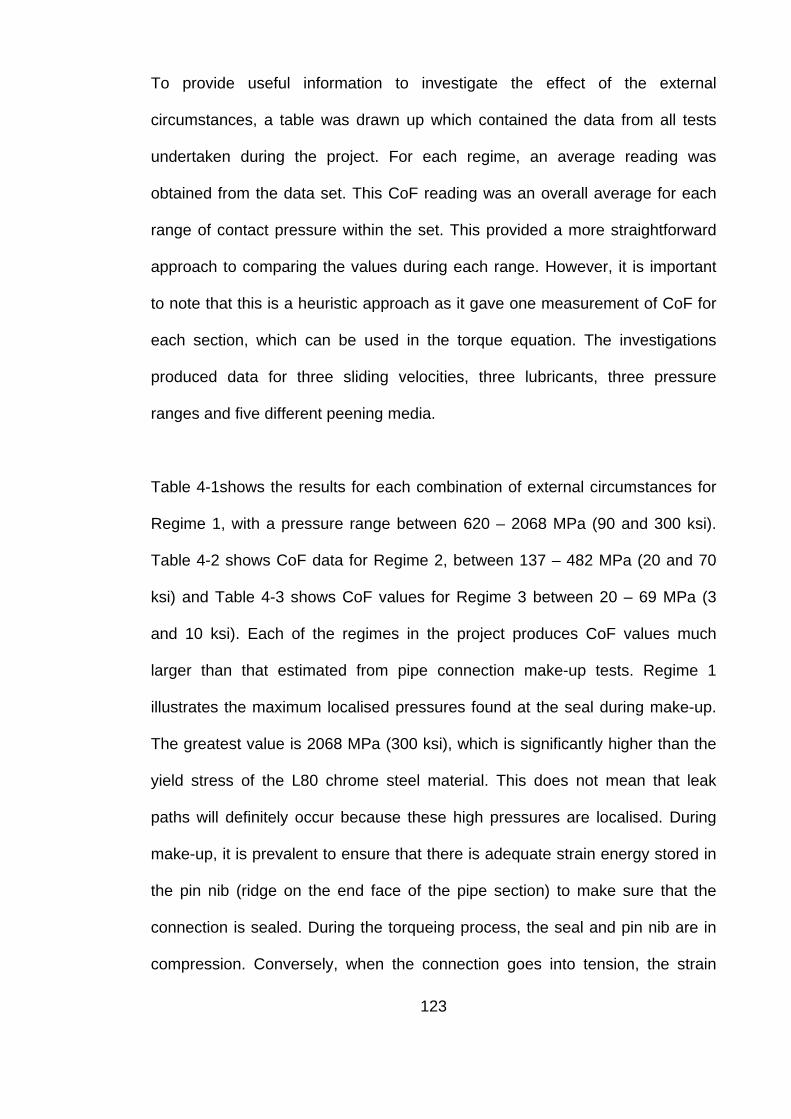
To provide useful information to investigate the effect of the external
circumstances, a table was drawn up which contained the data from all tests
undertaken during the project. For each regime, an average reading was
obtained from the data set. This CoF reading was an overall average for each
range of contact pressure within the set. This provided a more straightforward
approach to comparing the values during each range. However, it is important
to note that this is a heuristic approach as it gave one measurement of CoF for
each section, which can be used in the torque equation. The investigations
produced data for three sliding velocities, three lubricants, three pressure
ranges and five different peening media.
Table 4-1shows the results for each combination of external circumstances for
Regime 1, with a pressure range between 620 – 2068 MPa (90 and 300 ksi).
Table 4-2 shows CoF data for Regime 2, between 137 – 482 MPa (20 and 70
ksi) and Table 4-3 shows CoF values for Regime 3 between 20 – 69 MPa (3
and 10 ksi). Each of the regimes in the project produces CoF values much
larger than that estimated from pipe connection make-up tests. Regime 1
illustrates the maximum localised pressures found at the seal during make-up.
The greatest value is 2068 MPa (300 ksi), which is significantly higher than the
yield stress of the L80 chrome steel material. This does not mean that leak
paths will definitely occur because these high pressures are localised. During
make-up, it is prevalent to ensure that there is adequate strain energy stored in
the pin nib (ridge on the end face of the pipe section) to make sure that the
connection is sealed. During the torqueing process, the seal and pin nib are in
compression. Conversely, when the connection goes into tension, the strain
123

energy is necessary to ensure the two surfaces remain in contact and maintain
a seal.
Connections can be exposed to both tension and compression and therefore
there is a large variation in the pressure that they are exposed to. A comparison
between the localised contact pressures during the internal compression
(shown in Figure 4-1) and external tension shown in Figure 4-2) shows the
significant difference between the stresses acting on the seal during make-up.
These stresses are simulated using Finite Element analysis of the area of
sealing between the pipe and coupling. The highest values of stress were
located on the seal. The differences mean that to ensure no leak paths occur, a
seal must not be broken after the torque has been applied. If the value of
contact pressure reduces considerably during the make-up process then a seal
will not be maintained; this has the opportunity to cause major problems when it
comes to subsea operation.
The differences between the stresses during make-up mean that the
connections need to seal in both tension and compression; therefore the
accuracy of the connection dimensions needs to be precise. The torque value
used to make-up the connection also needs to be determined accurately.
Problems have occurred in the past due to the connections being contaminated,
or an insufficient amount of lubricant applied during make-up. Although these
failures are not caused by the design and are entirely due to the assembly of
the connections offshore, this project provides an understanding of how
differences in the lubrication or surface roughness can affect CoF. Unwanted
124

dust or dirt particles can result in an uneven surface which can produce scratch
marks during make-up, hence increasing the wear rate. This may also increase
CoF leading to a larger torque being required to make-up the connection
properly.
Figure 4-1: Contact stress during internal compression of connection during make-up (32)
(ksi
)
125
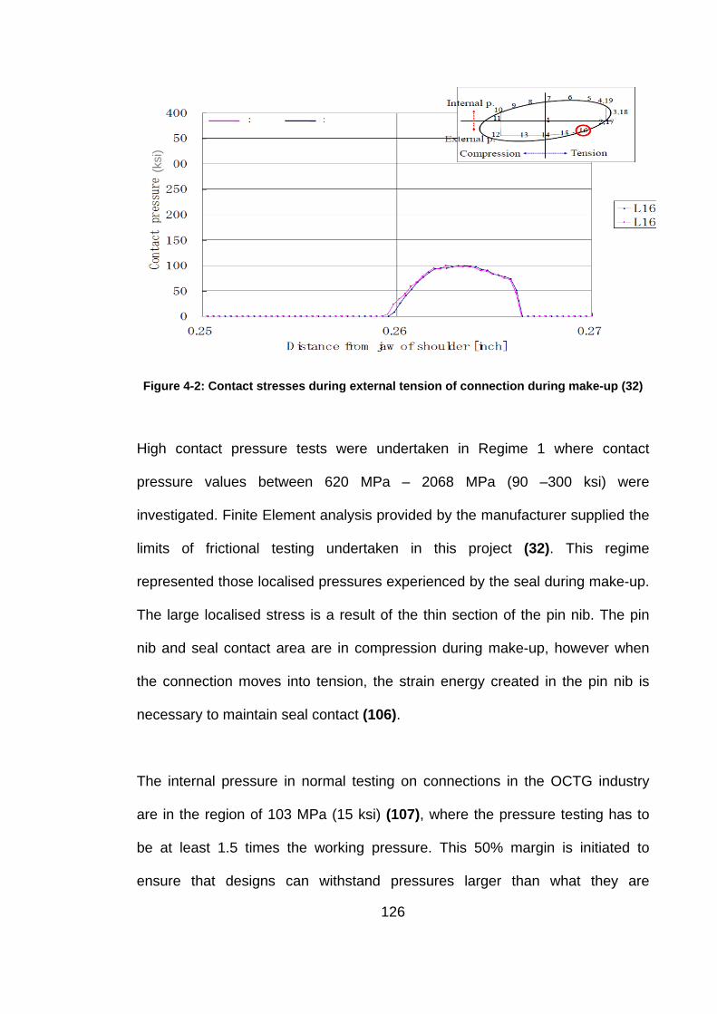
Figure 4-2: Contact stresses during external tension of connection during make-up (32)
High contact pressure tests were undertaken in Regime 1 where contact
pressure values between 620 MPa – 2068 MPa (90 –300 ksi) were
investigated. Finite Element analysis provided by the manufacturer supplied the
limits of frictional testing undertaken in this project (32). This regime
represented those localised pressures experienced by the seal during make-up.
The large localised stress is a result of the thin section of the pin nib. The pin
nib and seal contact area are in compression during make-up, however when
the connection moves into tension, the strain energy created in the pin nib is
necessary to maintain seal contact (106).
The internal pressure in normal testing on connections in the OCTG industry
are in the region of 103 MPa (15 ksi) (107), where the pressure testing has to
be at least 1.5 times the working pressure. This 50% margin is initiated to
ensure that designs can withstand pressures larger than what they are
(ksi
)
126
designed to, in case of overload. This remains true for conditions where the
internal pressure (or rated pressure) of a system is 69 MPa (10 ksi).The values
of contact pressure investigated in this project are mainly based on localised
maximum pressure. Although the average contact pressure may be significantly
smaller than the values investigated here, small sections of the connection
could experience this much larger pressure.
The Regime 2 tests are in line with the contact conditions in loading flanks of
threads, where the average pressure is in the range of 137 – 482 MPa (20-70
ksi). The initial surface of the samples was rougher because they were cut from
a turned pipe. This does reflect the surface finish on the pipe end thread. The
CoF results are more sensitive to initial surface treatment and sliding speed (as
shown in Table 4-2). Regime 3 tests were only conducted on one surface
treatment due to the availability of test samples. The effect of sliding speed can
be seen in Table 4-3. By directly comparing these results with those obtained
by the American Petroleum Institute (API), there is no correlation. This is
because the two test procedures are not comparable due to their geometrical
differences. The results will be discussed in terms of surface treatment, sliding
distance, sliding speed and lubrication below.
127

Table 4-1: Regime 1 CoF data summary
Regime 1
Peening media
Ra
(µm)
[µ inch]
Contact
Pressure
MPa
[ksi]
Sliding
Velocity
(mm/s)
Lubricant A
/bronze plated
CoF
As-machined
chrome
0.7
[28]
620-
2068[90-
300]
3 0.127
15 0.111
50 0.117
Ceramic peened
chrome
1.52
[62]
620-2068
[90-300]
3 0.147
15 0.148
50 0.139
Coarser stainless
steel peened
chrome
0.81
[33]
620-2068
[90-300]
3 0.150
15 0.134
50 0.150
Al2O3 peened
chrome
2.45
[100]
620-2068
[90-300]
3 0.170
15 0.180
50 0.187
Finer stainless
steel peened
chrome
1.45
[47]
620-2068
[90-300]
3 0.142
15 0.133
50 0.121
128
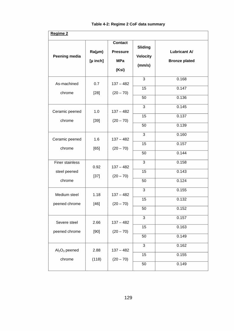
Table 4-2: Regime 2 CoF data summary
Regime 2
Peening media Ra(µm)
[µ inch]
Contact
Pressure
MPa
(Ksi)
Sliding
Velocity
(mm/s)
Lubricant A/
Bronze plated
As-machined
chrome
0.7
[28]
137 – 482
(20 – 70)
3 0.168
15 0.147
50 0.136
Ceramic peened
chrome
1.0
[39]
137 – 482
(20 – 70)
3 0.145
15 0.137
50 0.139
Ceramic peened
chrome
1.6
[65]
137 – 482
(20 – 70)
3 0.160
15 0.157
50 0.144
Finer stainless
steel peened
chrome
0.92
[37]
137 – 482
(20 – 70)
3 0.158
15 0.143
50 0.124
Medium steel
peened chrome
1.18
[46]
137 – 482
(20 – 70)
3 0.155
15 0.132
50 0.152
Severe steel
peened chrome
2.66
[90]
137 – 482
(20 – 70)
3 0.157
15 0.163
50 0.149
Al2O3 peened
chrome
2.88
(118)
137 – 482
(20 – 70)
3 0.162
15 0.155
50 0.149
129

Table 4-3: Regime 3 CoF data summary
Regime 3
Peening
media
Ra
(µm)
[µ inch]
Contact
Pressure
MPa
[ksi]
Sliding
Velocity
(mm/s)
Lubricant A/
bronze plated
Ceramic
peened
carbon
2.1
[82]
20 – 69
[3 – 10]
3 0.155
15 0.162
50 0.160
4.2 Effect of surface topography on CoF
By analysing the physical results obtained in this project, it was found that there
is a general trend of CoF with surface roughness in both Regime 1 and 2 tests
(c.f. Table 4-1 and 4-2). It is found that the CoF increases slightly with
increasing surface roughness for tests undertaken using the Lubricant A and
the bronze plated sample (see Figure 4-4). The results of this work show that
the higher the arithmetic average surface roughness, the higher the CoF. There
are however some exceptions to the rule.
The original conclusion behind this relationship between surface roughness and
CoF is due to the size and shape of the peening media that was used to create
a rougher surface. The area of the depressions on the material is dependent on
the size of the peening media. The larger peening media, such as coarse
stainless steel and ceramic beads, resulted in a surface which had larger
troughs. The shape and hardness of the peening media also played some part
in the value of CoF. The Metal Improvement Company (108) stated that the
130
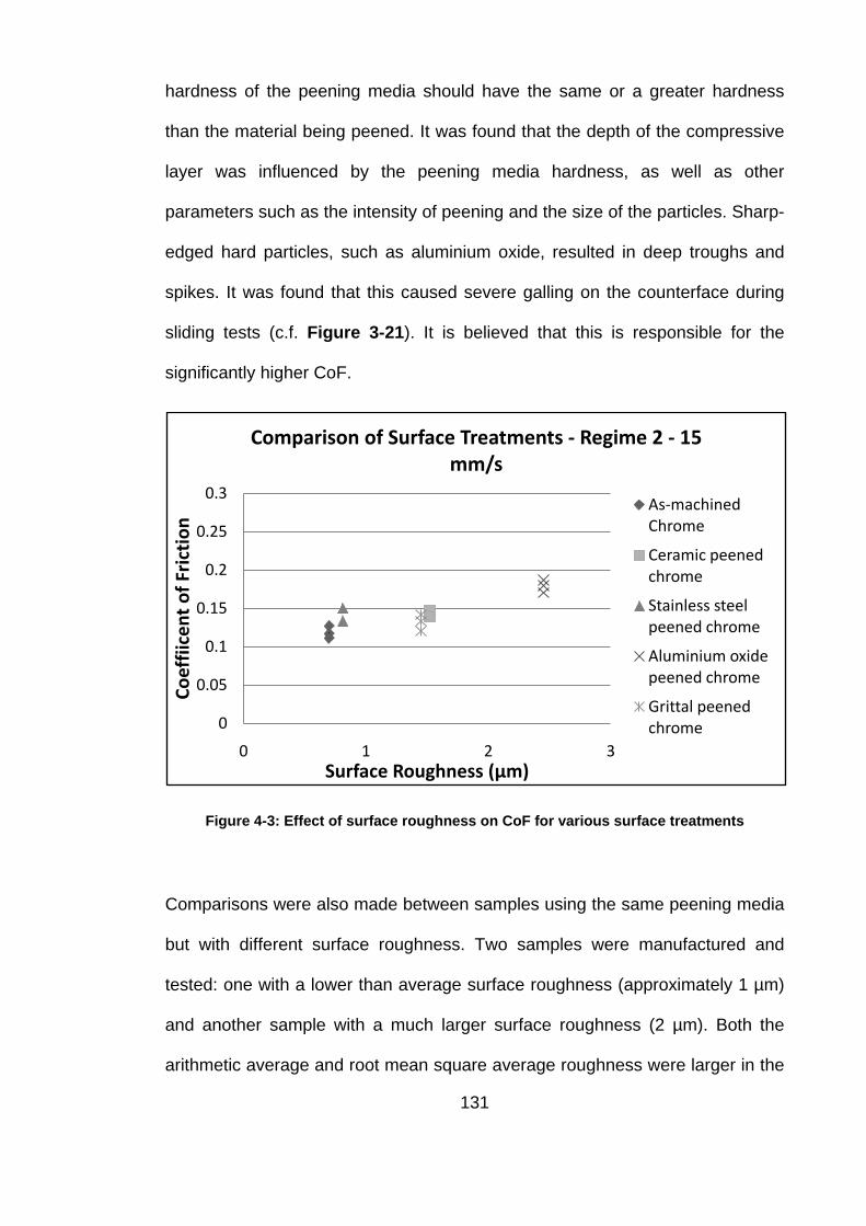
hardness of the peening media should have the same or a greater hardness
than the material being peened. It was found that the depth of the compressive
layer was influenced by the peening media hardness, as well as other
parameters such as the intensity of peening and the size of the particles. Sharp-
edged hard particles, such as aluminium oxide, resulted in deep troughs and
spikes. It was found that this caused severe galling on the counterface during
sliding tests (c.f. Figure 3-21). It is believed that this is responsible for the
significantly higher CoF.
Comparisons were also made between samples using the same peening media
but with different surface roughness. Two samples were manufactured and
tested: one with a lower than average surface roughness (approximately 1 µm)
and another sample with a much larger surface roughness (2 µm). Both the
arithmetic average and root mean square average roughness were larger in the
Figure 4-3: Effect of surface roughness on CoF for various surface treatments
0
0.05
0.1
0.15
0.2
0.25
0.3
0 1 2 3
Coef
fiice
nt o
f Fric
tion
Surface Roughness (µm)
Comparison of Surface Treatments - Regime 2 - 15 mm/s
As-machined Chrome
Ceramic peened chrome
Stainless steel peened chrome
Aluminium oxide peened chrome
Grittal peened chrome
131
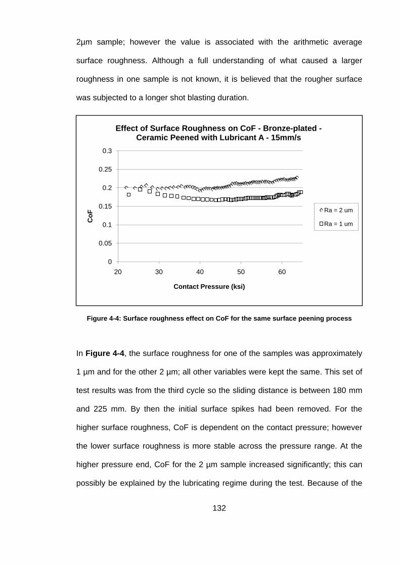
2µm sample; however the value is associated with the arithmetic average
surface roughness. Although a full understanding of what caused a larger
roughness in one sample is not known, it is believed that the rougher surface
was subjected to a longer shot blasting duration.
Figure 4-4: Surface roughness effect on CoF for the same surface peening process
In Figure 4-4, the surface roughness for one of the samples was approximately
1 µm and for the other 2 µm; all other variables were kept the same. This set of
test results was from the third cycle so the sliding distance is between 180 mm
and 225 mm. By then the initial surface spikes had been removed. For the
higher surface roughness, CoF is dependent on the contact pressure; however
the lower surface roughness is more stable across the pressure range. At the
higher pressure end, CoF for the 2 µm sample increased significantly; this can
possibly be explained by the lubricating regime during the test. Because of the
0
0.05
0.1
0.15
0.2
0.25
0.3
20 30 40 50 60
CoF
Contact Pressure (ksi)
Effect of Surface Roughness on CoF - Bronze-plated -Ceramic Peened with Lubricant A - 15mm/s
Ra = 2 um
Ra = 1 um
132

low sliding speed, the hydrodynamic effect is not significant. However some
lubricant could be entrapped in the shot peened pits. At the higher pressure end
in both circumstances, most of the lubricant will escape through the porous
contact interface because the contact pressure between the two samples is
highest at this point. In the 1 µm sample, the pits have a smaller diameter,
decreasing the likelihood of the lubricant squeezing out. In the 2 µm sample
there is more opportunity for the pits to join up, thus allowing faster leakage of
the lubricant. This is supported by the experimental outcomes noted by Ford
(35). The author noted that during the numerical modelling of the elastic contact
between rough surfaces, the shape of the asperities is taken to be non-
spherical and asymmetric. This is in contrast to the Greenwood-Williamson
model (50). Nevertheless, the GW results are coherent with Ford’s outcomes
which concluded that where the asperities were larger, there was a faster
lubricant spill out. An investigation into the effect of the direction of elongated
asperities was done. It was found that CoF was higher when testing was
undertaken in the direction of extended asperities, compared to situations
where the asperity length was smaller. The main conclusion of Ford’s
experiment proved that CoF increased with increasing surface roughness;
although the solutions were obtained purely using computer generated
experimental data.
4.3 Evolution of surface roughness with sliding distance
To investigate the behaviour of the surface roughness during testing, a ceramic
peened top sample with a bronze plate bottom sample test was undertaken with
Lubricant A. These results were obtained using the Regime 2 testing procedure.
133

The testing procedure was identical to the previous test, however between each
cycle the roughness of both surfaces were measured. For one ceramic peened
surface, the initial surface roughness was approximately 2.7 µm and for the
bronze plate surface, its value was also approximately 2.7 µm.
Figure 4-5 shows the arithmetic average surface roughness for the sample at
different sliding distances. A roughness measurement was taken at the
minimum and maximum pressure for each cycle. The change in topography and
reduction in roughness is almost immediate. After the first loading cycle, it
reduces to approximately 0.76 µm (30% of the initial value). A similar analysis
was done for the bronze plated surface.
Figure 4-6 shows the surface roughness values taken on the bronze plated
bottom sample at the same time as the ceramic peened surface shown above.
There is limited change in the surface roughness value before and during the
testing procedure. The first observation is owing to surface burnishing which
occurs when the localised stresses are above the yield limit of the contact
materials. It makes the surfaces appear smoother and usually reduces the
surface roughness. The second observation is that scratch marks emerge
because the counterface is sliding along the length of its surface. The area of
interest is the same for both samples, however the ceramic peened surface pits
are almost completely removed during testing because the contact is stationary
on the fixed area. It is believed that this is responsible for the reduction in CoF
after the first cycle. The spikes on the peened surface are worn very quickly
under such high contact pressure so that there is less galling or direct metal-to-
134

metal contacts. Therefore CoF is reduced and stabilised after the first cycle.
This will be discussed in detail later.
Figure 4-5: Surface roughness (Ra) values between cycles
Figure 4-6: Surface roughness (Ra) values between cycles
0
0.5
1
1.5
2
2.5
3
3.5
0 50 100 150 200 250 300
Surf
ace
Rou
ghne
ss, R
a (µ
m)
Sliding Distance (mm)
Roughness of ceramic peened surface during testing - 3mm/s
0
0.5
1
1.5
2
2.5
3
0 50 100 150 200 250 300
Surf
ace
Rou
ghne
ss, R
a (µ
m)
Sliding Distance (mm)
Roughness of Bronze-plated surface during testing - 3mm/s
135

4.4 Effect of sliding speed and contact regime on CoF
From the physical testing performed in this project, CoF reduces as the sliding
speed of contact between the two surfaces increases. This is usually caused by
hydrodynamic lubrication when there is a lubricant in contact. CoF depends on
the conditions that a system experiences; this includes but is not limited to the
material type, surface quality, lubrication, speed, pressure and the type of
contact. If the same types of test are undertaken but the velocity of travel
between two samples increases, then the dynamics of the contact changes. As
the velocity increases, the samples move past one another more rapidly. When
this happens, the shear stress of most metals will increase leading to a higher
tangential force. Conversely, more lubricant will be entrained into the asperity-
to-asperity contact so the hydrodynamic lubrication improves. The extent of
reduction of CoF with increasing speed is low in Regime 1 (c.f. Table 4-1);
however it does show to alter slightly for some combinations of surface
conditions. This is much more prevalent in the Regime 2 results reported above
(c.f. Table 4-2).
The three sliding velocities were selected to represent the tangential velocity of
the connection during the make-up. The industry produces a range of sizes of
connections from 2” 3/8 to 9” 7/8. It was important to establish whether the
make-up speed affected the CoF experienced by the surfaces, to ensure that
the value of torque was calculated accurately. The connection could be made
up between 1 and 4 RPM. The sliding speed, 𝑽𝑽, is equal to 𝑽𝑽 = 𝝅𝝅.𝒅𝒅.𝑻𝑻 (where 𝒅𝒅
is the diameter and 𝑻𝑻 is the rotation speed) and changes from 3 to 12.5 mm/s if
made-up at 1 RPM.
136

Figure 4-7 shows the CoF values for Regime 2 which is the medium pressure
range. This regime includes tests with contact pressure between 20 and 70 ksi
(137 - 482 MPa). Similar to Regime 1, in most cases, an increase in sliding
speed reduces CoF. The effect of sliding speed on CoF was relatively low for
the three speeds investigated because the speeds are relatively similar. Larger
differences in sliding speeds may have been more of an impact because there
is an increased chance for hydrodynamic lubrication to be experienced by the
surfaces over larger ranges. However, as the connection will not experience
speeds higher than 50 mm/s, increasing it was outside the scope of the project.
Figure 4-7: Comparison of three lubricants for Regime 2 tests
This shows a comparison between the three pressure regimes. The highest
value of CoF occurs in Regime 3, within the lowest pressure regime. It was
0
0.05
0.1
0.15
0.2
0.25
0.3
0 50 100 150 200 250
Coe
ffici
ent o
f Fric
tion
Contact Pressure (ksi)
Ceramic peened / Bronze-plate / Propietary Lubricant
3mm/s
15mm/s
50mm/s
137
expected that at the lowest pressure, there would be limited asperity-to-asperity
contact, and therefore the load would be mainly carried by the lubricant. This
could be due to the surface of those samples, which are not worn out as easily
as those in Regimes 1 and 2 under higher contact pressure. CoF remains high
in the second and third cycle, so the average of three cycles reported above
becomes higher than those in Regimes 1 and 2. Whereas, in Regime 1 and 2
tests, the surface asperities were removed within the first cycle so that the CoF
stabilises at a lower level.
Figure 4-7 also shows the effect of sliding speed on CoF in three different
contact regimes. There was very little change between the CoF with
modifications of speed at very low pressures shown in Regime 3. There is
however a small reduction in CoF with increasing speeds in both Regimes 1
and 2.
According to Coulomb’s and Amontons’ laws of friction, the sliding frictional
force is independent of sliding velocity (3). This is predominantly true for cases
of dry friction. Work done by Zwörner et al (109) looked at the effect of sliding
velocity in point contact between different types of carbon compounds. The
main outcome was that the frictional forces were independent of the sliding
velocity even in instances of significantly lower speeds. The results were
obtained using a friction force microscope which allowed the frictional forces to
be investigated on a nano-scale. The research was based on the understanding
that the tip moves with stick-slip type movement. During the slip section, the tip
experienced very high speeds, and in the stick portion, it was stationary. It was
138
determined that as long as the slip movement of the tip of the microscope is
faster than the sliding velocity, the friction will be independent of speed. It is
important to note however, that this is only true when there is no lubrication
between the two samples in contact. The velocities in Zwörner’s tests are in the
region of 50 to 800 times smaller than the velocity experienced by the surfaces
during make-up of the connection, so this may explain the significant
differences in CoF.
Investigation by Wang et al (110) showed that as the speed increased, both the
wear rate and friction coefficient reduced. This was a consequence of the higher
speeds producing a more efficient lubricating regime. This backs up the results
experienced in this work, and the reason that in some tests CoF did not reduce
may be because the efficiency of the lubricating regime did not improve. In the
case of Regime 3, where the pressure was so low, an increase in speed did not
make any difference to how the surface asperities reacted. This confirms that
the hydrodynamic lubrication is not significant and that the mechanism is mainly
boundary lubrication. It is noted that the surface roughness of the samples for
Regime 3 tests is higher (c.f. Table 4-3) which facilitates side leakage during
sliding. The effect of hydrodynamic pressure on the asperity flattening, or wear,
is insignificant.
4.5 Effect of sliding distance on the CoF
The graphs in Figure 4-8 to Figure 4-10 show the effect of the sliding distance
on CoF for a bronze plated surface with Lubricant A and ceramic peened
arrangement. Initially, CoF is much higher than the average value and this
139

reduces as the sliding distance increases. At this point the CoF value levels out
for the rest of the sliding distance. The initial surface roughness is significantly
larger than the final roughness for the peened surface. The plated surface
(bronze plated in this case) maintains a stable surface roughness throughout
the entire testing method. The high CoF value in the first stroke of sliding is
inferring the existence of galling and direct metal-to-metal contact.
Figure 4-8: Effect of sliding distance on CoF at 3mm/s
0
0.05
0.1
0.15
0.2
0.25
0.3
0 50 100 150 200 250 300
CoF
Sliding Distance (mm)
CoF versus Sliding Distance for Ceramic peened chrome - Bronze-plate chrome steel - 3 mm/s - Regime 1
140
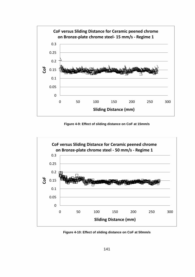
Figure 4-9: Effect of sliding distance on CoF at 15mm/s
Figure 4-10: Effect of sliding distance on CoF at 50mm/s
0
0.05
0.1
0.15
0.2
0.25
0.3
0 50 100 150 200 250 300
CoF
Sliding Distance (mm)
CoF versus Sliding Distance for Ceramic peened chrome on Bronze-plate chrome steel- 15 mm/s - Regime 1
0
0.05
0.1
0.15
0.2
0.25
0.3
0 50 100 150 200 250 300
CoF
Sliding Distance (mm)
CoF versus Sliding Distance for Ceramic peened chrome on Bronze-plate chrome steel - 50 mm/s - Regime 1
141

This initial high CoF is much more dominant at the lowest speed. This is due to
the fact that very little lubricant can be present in initial asperity contacts
reducing the effectiveness of boundary lubrication. As the speed increases, a
thin layer of lubricant can be entrained into the asperity contact improving the
effectiveness of boundary lubrication. At each of the three speeds, CoF is
higher for only a section of the first stroke, before stabilising for the remainder of
the strokes; concurrently, the surface roughness reduces. Therefore, it is
plausible to conclude that the lubrication improves as the sharp asperities are
flattened. The general trend is similar to the work by Le et al (111) in the mixed
lubrication regime in cold metal forming. Although the surface roughness in this
case is much lower than that of the ceramic peened surface, there are
similarities between the two. In the results of this project, the troughs become
increasingly more isolated from one another and, compared with the linked
valleys, the contact pressure in the valleys is much higher. However, it is
assumed here that asperity crushing terminates when the asperity contact
percolation is reached. Nevertheless, the only evidence to support this is that
the initial surface roughness is very high; then after the first stroke and the
subsequent strokes, the surface roughness levels out to a stable value. The
bronze plated surface retains the same value of roughness after testing. From
the surface images it can be shown (in Chapter 4 that the majority of this
surface remains unchanged and only a thin wear mark is present on the surface
after being tested. After the initial peened surface is burnished, the coefficient of
friction is typical of the boundary lubrication mechanism.
142
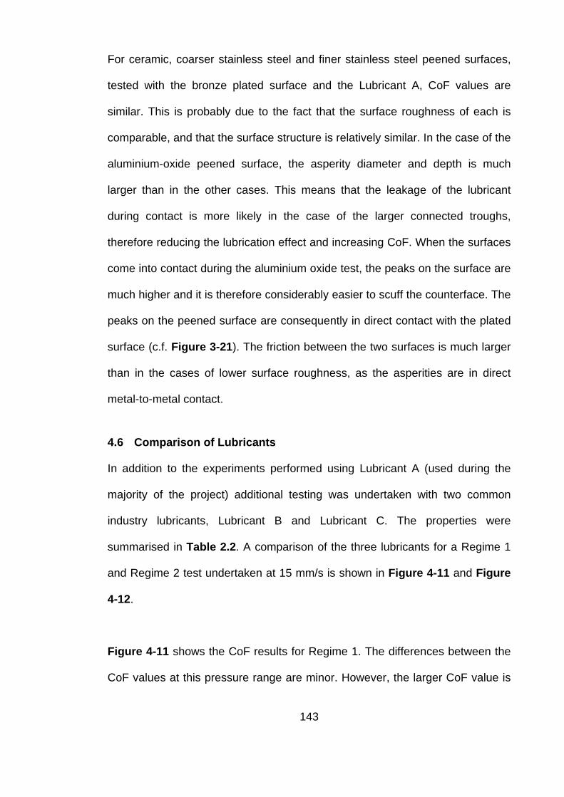
For ceramic, coarser stainless steel and finer stainless steel peened surfaces,
tested with the bronze plated surface and the Lubricant A, CoF values are
similar. This is probably due to the fact that the surface roughness of each is
comparable, and that the surface structure is relatively similar. In the case of the
aluminium-oxide peened surface, the asperity diameter and depth is much
larger than in the other cases. This means that the leakage of the lubricant
during contact is more likely in the case of the larger connected troughs,
therefore reducing the lubrication effect and increasing CoF. When the surfaces
come into contact during the aluminium oxide test, the peaks on the surface are
much higher and it is therefore considerably easier to scuff the counterface. The
peaks on the peened surface are consequently in direct contact with the plated
surface (c.f. Figure 3-21). The friction between the two surfaces is much larger
than in the cases of lower surface roughness, as the asperities are in direct
metal-to-metal contact.
4.6 Comparison of Lubricants
In addition to the experiments performed using Lubricant A (used during the
majority of the project) additional testing was undertaken with two common
industry lubricants, Lubricant B and Lubricant C. The properties were
summarised in Table 2.2. A comparison of the three lubricants for a Regime 1
and Regime 2 test undertaken at 15 mm/s is shown in Figure 4-11 and Figure
4-12.
Figure 4-11 shows the CoF results for Regime 1. The differences between the
CoF values at this pressure range are minor. However, the larger CoF value is
143

for Lubricant A, which is of similar trend to Regime 2. In all cases, the CoF is
initially higher and then decreases significantly. This is associated with surface
burnishing explained in section 4.5. The initial high CoF was owing to galling
due to the rough shot peened surface. Once the surface is burnished, the CoF
becomes stable which is typical of boundary lubrication.
Figure 4-12 shows a similar overall CoF value for the two commercial lubricants
compared to Lubricant A. Comparing the three, Lubricant B containing the metal
particles has the lowest CoF. This could be caused by the fragments of metal
filling gaps on the surface and producing more effective boundary lubrication. It
is well known that metal particles such as lead or zinc have good stiction to
steel surfaces and may generate a thin coating on the contacting surfaces
avoiding direct metal-to-metal contact. Therefore Lubricant B provides effective
boundary lubrication. Lubricant C contains a large amount of non-metallic solid
lubricants which also generates a transfer layer on the peened surface. The
CoF is similar to that of B. Although Lubricant A produces a higher CoF, it is
stable after a short sliding distance. It is believed that the boundary additives
would react with the fresh surface generated by mild galling. The CoF would
have stabilised within the first make-up in a premium tubular connection and it
does have the advantage of being environmentally friendly and less detrimental
to the well.
It is noted that the decrease of CoF in Regime 2 is much slower than in Regime
1. This infers that the surface burnishing is slower in Regime 2 than Regime 1
due to the lower contact pressure.
144
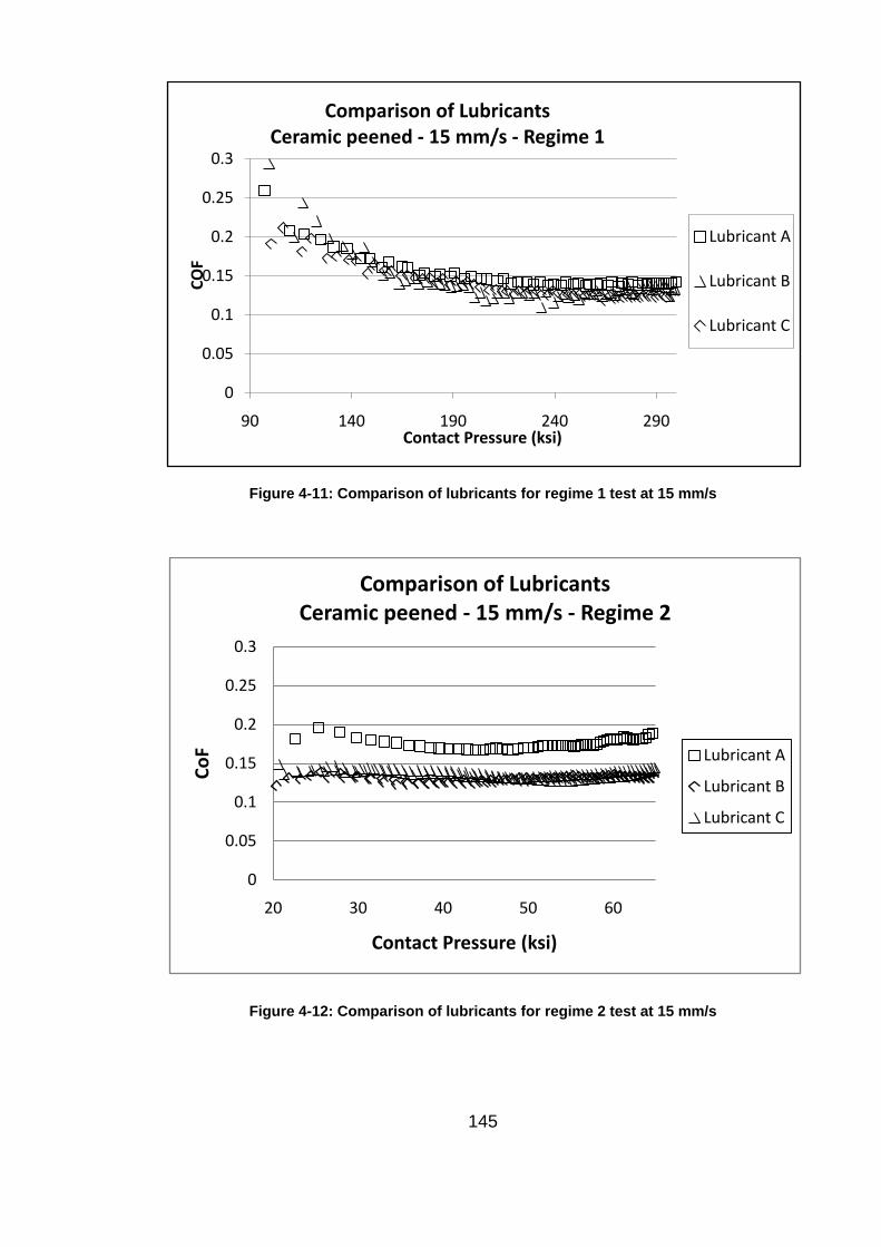
Figure 4-11: Comparison of lubricants for regime 1 test at 15 mm/s
Figure 4-12: Comparison of lubricants for regime 2 test at 15 mm/s
0
0.05
0.1
0.15
0.2
0.25
0.3
90 140 190 240 290
COF
Contact Pressure (ksi)
Comparison of Lubricants Ceramic peened - 15 mm/s - Regime 1
Lubricant A
Lubricant B
Lubricant C
0
0.05
0.1
0.15
0.2
0.25
0.3
20 30 40 50 60
CoF
Contact Pressure (ksi)
Comparison of Lubricants Ceramic peened - 15 mm/s - Regime 2
Lubricant A
Lubricant B
Lubricant C
145
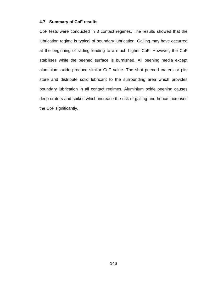
4.7 Summary of CoF results
CoF tests were conducted in 3 contact regimes. The results showed that the
lubrication regime is typical of boundary lubrication. Galling may have occurred
at the beginning of sliding leading to a much higher CoF. However, the CoF
stabilises while the peened surface is burnished. All peening media except
aluminium oxide produce similar CoF value. The shot peened craters or pits
store and distribute solid lubricant to the surrounding area which provides
boundary lubrication in all contact regimes. Aluminium oxide peening causes
deep craters and spikes which increase the risk of galling and hence increases
the CoF significantly.
146

Chapter 5 : Modelling of Tribological Contact between
Surfaces during Make-up Process
5.1 Modelling of tribological contact
One of the main objectives of the project was to develop a working model,
capable of predicting the tribological behaviour of the contact between the
surfaces in a premium tubular connection during the make-up process. In order
to achieve this, some assumptions concerning the behaviour of the surfaces
and generalisations regarding the material properties were also implemented.
The friction, wear and surface roughness predictions from the modelling are
presented. The solutions were validated using physical test results (found in
Chapter 4).
To offer understanding of the experimental results, computer modelling is used
as a method of cost efficiently simulating how variations in input affect the
conclusions. Furthermore, they permit additional information to be added,
allowing the estimation of supplementary results. If these methods can be
corroborated, then the model can be used to predict outcomes in situations
where a large scale physical test would be time and cost inefficient. Estimations
using matrices of mathematical calculations have been around for centuries;
however with the addition of large processing powers, computer simulations
provide a much quicker and more accurate solutions. Computer modelling can
be done in many different ways, including using software akin to MATLAB which
manipulate matrices of data or by using Finite Element analysis (FEA) such as
ANSYS or ABAQUS. The latter provides a solution where each point (or node)
147

in a model is defined by a series of equations and properties. A model was
produced using the software to represent an object or surface of interest and at
each point, a set of unknowns and equations are defined. These nodal
calculations are subsequently computed to create a full scale model of results.
Finite Element analysis can give very accurate results, however the computer
processing power and memory required to obtain results in a reasonable time
are very large. In order to obtain the most accurate models, each node in a
simulation has to represent the subject.
Although useful, FEA can be time consuming and highly complex systems
prove difficult to model. An alternative modelling method uses MATLAB (or
Matrix Laboratory), which is a numerical computing program produced by
MathWorks (112). It is a software language that can provide an interactive
setting in which programming, numerical computation and visualisation of
matrices can be achieved. To obtain a solution, input data is entered as
matrices. These matrices are processed by means of user-defined equations
and all data is analysed to obtain an accurate solution to the problem. Instead of
calculating only one value at a time (as done in traditional situations), the matrix
allows a set of inputs to be computed. This is useful for situations where the
values change or, in the case of material properties, where the height profile of
a surface can be included in the calculation. The main disadvantage of this
method is in the time taken to develop the program; however it does produce a
far more accurate estimation of the project being investigated.
148

The three-dimensional surface readings obtained using the laser confocal
microscopes (in Chapter 3) included a matrix of height profile. This meant that
the roughness and surface profile after testing could be estimated using the
correct equations and input of material properties. The surface profiles were
measured both prior to, and after each cycle and following the frictional testing.
These sets of data allowed experimental results to be compared with modelled
data. In addition to this, the wear rate and wear volume could be estimated
alongside to the coefficient of friction. This model has the capability to be very
valuable in the future. It offers a potential tool which could be used by the
operator, to understand and make appropriate changes to the torque value
used during make-up, which would compensate for changes in operational
conditions.
5.2 Wear model for surface burnishing
A wear model was created to allow the prediction of surface roughness
variation, wear volume and actual wear area for a premium tubular connection.
This model could be used to improve the calculation of torque for the make-up
process in the oil and gas field. Connection make-up is where a pipe end is
screwed into a coupling using a bucking unit which is controlled by a pre-
defined torque value. In order to obtain this value, a CoF value is entered into a
torque equation. The accuracy of CoF is significant because it is a major
contribution in the torque computation equation (shown in Equation 1.11).
However, since the current method of calculating the CoF does not take into
account changes caused by the wearing of the surface, the value used could
potentially cause under-torqueing or over-torqueing of the connection. The
149
program, in theory, could eliminate this problem by allowing a more precise
estimation of CoF, which in turn would result in a more accurate torque value.
Being able to quantify and estimate this change in CoF could essentially provide
a far more accurate value which in high-temperature, high-pressure
circumstances could be the difference between a connection leaking or not.
This reduces the opportunity for leak paths to occur at very high pressures and
temperatures.
5.2.1 Archard's wear theorem
Wear occurs when two moving surfaces come into contact. The rate of wear
and the amount of material removed during the sliding motion depends entirely
on the situation that the two materials are in. Wear is also dependent on the
type of lubrication that is experienced by the contact surfaces. Wear, friction
and lubrication are dependent on each other. A classic wear model was based
on Archard’s theorem in which the wear resistance is proportional to the
materials’ hardness (113). Archard stated that:
𝑽𝑽𝒔𝒔
= 𝒌𝒌𝑭𝑭𝑵𝑵𝑯𝑯
(5.1)
Where 𝑽𝑽 is the wear volume; 𝒔𝒔 is the sliding distance; 𝒌𝒌, the dimensionless
wear rate which was used as a fitting parameter in the program; 𝑭𝑭𝑵𝑵, the normal
load; and 𝑯𝑯 the hardness of the worn surface. This means that the wear volume
is directly proportional to the normal force and inversely proportional to the
hardness of the worn material (in this case the peened surface which is the 150
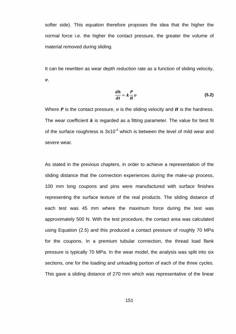
softer side). This equation therefore proposes the idea that the higher the
normal force i.e. the higher the contact pressure, the greater the volume of
material removed during sliding.
It can be rewritten as wear depth reduction rate as a function of sliding velocity,
𝒗𝒗.
𝒅𝒅𝒉𝒉𝒅𝒅𝑻𝑻
= 𝒌𝒌𝟒𝟒𝑯𝑯𝒗𝒗 (5.2)
Where 𝟒𝟒 is the contact pressure, 𝒗𝒗 is the sliding velocity and 𝑯𝑯 is the hardness.
The wear coefficient 𝒌𝒌 is regarded as a fitting parameter. The value for best fit
of the surface roughness is 3x10⁻⁴ which is between the level of mild wear and
severe wear.
As stated in the previous chapters, in order to achieve a representation of the
sliding distance that the connection experiences during the make-up process,
100 mm long coupons and pins were manufactured with surface finishes
representing the surface texture of the real products. The sliding distance of
each test was 45 mm where the maximum force during the test was
approximately 500 N. With the test procedure, the contact area was calculated
using Equation (2.5) and this produced a contact pressure of roughly 70 MPa
for the coupons. In a premium tubular connection, the thread load flank
pressure is typically 70 MPa. In the wear model, the analysis was split into six
sections, one for the loading and unloading portion of each of the three cycles.
This gave a sliding distance of 270 mm which was representative of the linear
151
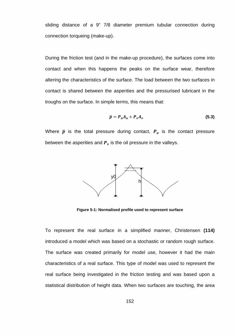
sliding distance of a 9” 7/8 diameter premium tubular connection during
connection torqueing (make-up).
During the friction test (and in the make-up procedure), the surfaces come into
contact and when this happens the peaks on the surface wear, therefore
altering the characteristics of the surface. The load between the two surfaces in
contact is shared between the asperities and the pressurised lubricant in the
troughs on the surface. In simple terms, this means that:
𝒑𝒑� = 𝟒𝟒𝒂𝒂𝑨𝑨𝒂𝒂 + 𝟒𝟒𝒗𝒗𝑨𝑨𝒗𝒗 (5.3)
Where 𝒑𝒑� is the total pressure during contact, 𝟒𝟒𝒂𝒂 is the contact pressure
between the asperities and 𝟒𝟒𝒗𝒗 is the oil pressure in the valleys.
Figure 5-1: Normalised profile used to represent surface
To represent the real surface in a simplified manner, Christensen (114)
introduced a model which was based on a stochastic or random rough surface.
The surface was created primarily for model use, however it had the main
characteristics of a real surface. This type of model was used to represent the
real surface being investigated in the friction testing and was based upon a
statistical distribution of height data. When two surfaces are touching, the area
y0 h
152

of “real” contact is only a portion of the nominal contact area (115). As contact
pressure is equal to the force divided by the area, the actual contact pressure
experienced on particular features (e.g. the peaks on the surface) is significantly
higher than initially expected. This also means that on certain sections,
particularly in the valleys of the asperities, the contact pressure is considerably
lower than first believed. As this is a highly researched area of tribology, there
are several techniques already available to investigate the contact area. To
calculate the contact area, a function was implemented in MATLAB. This
identified the surface height and shape of the asperities using statistical
analysis of a Christensen model.
Figure 5-2 shows an example of the real ceramic peened surfaces of the pipe
section used with the bronze plated surface and proprietary lubricant. These
images were constructed using an Olympus LEXT 3D confocal microscope.
Some shot blasting marks can be clearly observed on the surface and these
occur in a very random pattern. These marks are created by means of shot
blasting ceramic particles at the surface. This is used on the pipe section of the
connection. The machining marks are no longer visible and the surface
becomes almost isotropic compared the plated one.
153
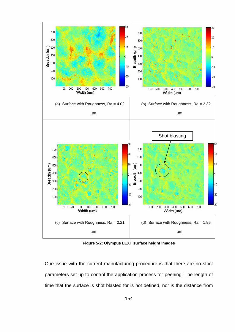
(a) Surface with Roughness, Ra = 4.02
µm
(b) Surface with Roughness, Ra = 2.32
µm
(c) Surface with Roughness, Ra = 2.21
µm
(d) Surface with Roughness, Ra = 1.95
µm
Figure 5-2: Olympus LEXT surface height images
One issue with the current manufacturing procedure is that there are no strict
parameters set up to control the application process for peening. The length of
time that the surface is shot blasted for is not defined, nor is the distance from
Shot blasting
154
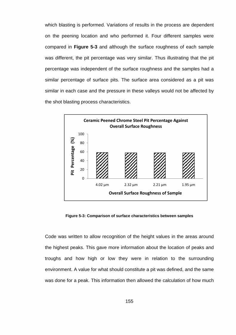
which blasting is performed. Variations of results in the process are dependent
on the peening location and who performed it. Four different samples were
compared in Figure 5-3 and although the surface roughness of each sample
was different, the pit percentage was very similar. Thus illustrating that the pit
percentage was independent of the surface roughness and the samples had a
similar percentage of surface pits. The surface area considered as a pit was
similar in each case and the pressure in these valleys would not be affected by
the shot blasting process characteristics.
Figure 5-3: Comparison of surface characteristics between samples
Code was written to allow recognition of the height values in the areas around
the highest peaks. This gave more information about the location of peaks and
troughs and how high or low they were in relation to the surrounding
environment. A value for what should constitute a pit was defined, and the same
was done for a peak. This information then allowed the calculation of how much
0
20
40
60
80
100
4.02 µm 2.32 µm 2.21 µm 1.95 µm
Pit
Perc
enta
ge (
%)
Overall Surface Roughness of Sample
Ceramic Peened Chrome Steel Pit Percentage Against Overall Surface Roughness
155

of the surface was a valley and how much was a peak. This allowed
conclusions of the ratio of valleys to peaks to be drawn.
Figure 5-4: Height data distribution for 4 ceramic peened chrome steel samples
Figure 5-4 shows a distribution of the surface height data for four samples with
different arithmetic average surface roughness values. Note that the total
number of pixels of each measurement is the same. For the sample with the
largest surface roughness, there are a larger number of higher peaks and
deeper troughs. This is expected because, in this case, the deeper pits were
probably produced due to larger peening media particles being blasted at the
surface. Where the peaks are higher, the material movement must have been
much larger than that of the smaller valleys and this movement of material
produced the larger peaks on the surface. In the case of the other samples, 156

where the surface roughness is similar (approximately 2 µm), the number of
baseline height values is higher and the number of larger peaks and troughs
reduces. This means that in the cases of lower roughness values, the height of
the surface is more concentrated around the base line which was altered by
peening.
5.2.2 Asperity flattening and percolation
From Williams’ “Engineering Tribology” (1) the load can be obtained using the
equation:
𝑾𝑾 = 𝒑𝒑� ∗ 𝝅𝝅𝟑𝟑 ∗ �𝟑𝟑𝑹𝑹𝟒𝟒𝑬𝑬∗
�𝟐𝟐 (5.4)
Where 𝒑𝒑� is the mean pressure, 𝑾𝑾 is the normal load acting on the surface, 𝑹𝑹 is
the reduced radius of contact and 𝑬𝑬∗ is the contact modulus. This equation was
proven to be applicable for elastic deformation of a surface. Provided that the
surface experiences elastic deformation, the following holds true.
Rearranging this gives the mean pressure to be:
𝒑𝒑� =𝟏𝟏𝝅𝝅∗ �
𝟏𝟏𝟏𝟏 ∗𝑾𝑾 ∗ 𝑬𝑬∗𝟐𝟐
𝟎𝟎 ∗ 𝑹𝑹𝟐𝟐�
𝟏𝟏𝟑𝟑
(5.5)
Work by Patir and Cheng (116) gave the following set of equations used to
calculate the lubricant characteristics in a contact between two rough surfaces.
Because the sliding speed is low, it is assumed that the lubricant flow rate, 𝒒𝒒𝒙𝒙,
is mainly driven by the pressure gradient as :
157
𝒒𝒒𝒙𝒙 = 𝝓𝝓𝒙𝒙𝒉𝒉𝑻𝑻
𝟑𝟑
𝟏𝟏𝟐𝟐𝟏𝟏𝒅𝒅𝟒𝟒𝒗𝒗𝒅𝒅𝒙𝒙
(5.6)
Where𝟏𝟏 is the oil viscosity, 𝒉𝒉𝑻𝑻 is the mean oil thickness, 𝟒𝟒𝒗𝒗 is the valley
lubricant pressure and 𝝓𝝓𝒙𝒙 is the flow factor per unit width.
The flow factor per unit width for a rough contact is calculated using the
equation:
𝝓𝝓𝒙𝒙 = �𝒂𝒂𝟐𝟐(𝑯𝑯𝑻𝑻 − 𝑯𝑯𝑻𝑻𝑭𝑭)𝟐𝟐 + 𝒂𝒂𝟑𝟑(𝑯𝑯𝑻𝑻 − 𝑯𝑯𝑻𝑻𝑭𝑭)𝟑𝟑�/𝒉𝒉𝑻𝑻𝟑𝟑 (5.7)
Where
𝑯𝑯𝑻𝑻𝑭𝑭 = 𝟑𝟑 ��𝟏𝟏 − �𝟎𝟎.𝟒𝟒𝟏𝟏𝟒𝟒𝟏𝟏𝟏𝟏 𝜸𝜸� � + 𝟏𝟏�−𝟎𝟎.𝟐𝟐𝟖𝟖𝟎𝟎𝟎𝟎𝟏𝟏
� (5.8)
𝒂𝒂𝟐𝟐 = 𝟎𝟎.𝟎𝟎𝟖𝟖𝟏𝟏𝟑𝟑𝟏𝟏𝟖𝟖(𝐥𝐥𝐥𝐥(𝟎𝟎𝜸𝜸))𝟑𝟑 − 𝟎𝟎.𝟎𝟎𝟎𝟎𝟏𝟏𝟏𝟏𝟎𝟎𝟎𝟎𝟏𝟏(𝐥𝐥𝐥𝐥(𝟎𝟎𝜸𝜸))𝟒𝟒 (5.9)
𝒂𝒂𝟑𝟑 = 𝟏𝟏.𝟎𝟎𝟎𝟎𝟏𝟏𝟎𝟎 − 𝟎𝟎.𝟏𝟏𝟏𝟏𝟎𝟎𝟐𝟐𝟏𝟏 𝐥𝐥𝐥𝐥(𝜸𝜸) + (𝟎𝟎.𝟎𝟎𝟒𝟒𝟏𝟏𝟖𝟖𝟖𝟖𝟑𝟑 𝐥𝐥𝐥𝐥(𝜸𝜸))𝟐𝟐
− (𝟎𝟎.𝟎𝟎𝟏𝟏𝟏𝟏𝟒𝟒𝟏𝟏𝟏𝟏 𝐥𝐥𝐥𝐥(𝜸𝜸))𝟑𝟑 (5.10)
Where 𝜸𝜸 is the Peklenik number which identifies the roughness pattern of the
surface, 𝑯𝑯𝑻𝑻 is the ratio of the average film thickness 𝒉𝒉𝑻𝑻 is the r.m.s surface
roughness 𝑹𝑹𝒒𝒒, 𝑯𝑯𝑻𝑻𝑭𝑭 is the percolation threshold value of 𝑯𝑯𝑻𝑻. It is a measure of the
remaining asperity height compared to initial surface height when the surface
valleys are isolated (117).
According to Hamrock and Dowson (118), the central lubricant film thickness
hcen with a point contact can be derived from the relationship
158

𝒉𝒉𝑭𝑭𝑻𝑻𝑻𝑻 = 𝟑𝟑.𝟑𝟑𝟒𝟒𝑹𝑹 �𝟏𝟏𝑫𝑫𝑬𝑬′𝑹𝑹
�𝟎𝟎.𝟏𝟏𝟒𝟒
�𝑾𝑾𝑬𝑬′𝑹𝑹𝟐𝟐
�−𝟎𝟎.𝟐𝟐𝟐𝟐
(5.11)
Whereη is the viscosity of the lubricant and u the entraining speed (in this case
half of the speed of sliding). The lubricant film thickness decreases with
increasing load and hence the increase in the ‘real’ asperity-to-asperity contact
ratio.
The ratio Λ of lubricant film thickness to combined r.m.s surface roughness is
often used as a lubrication parameter and given by
𝚲𝚲 =𝒉𝒉𝑭𝑭𝑻𝑻𝑻𝑻
�𝑹𝑹𝒒𝒒,𝟏𝟏𝟐𝟐 + 𝑹𝑹𝒒𝒒,𝟐𝟐
𝟐𝟐
(5.12)
Where Rq,1 is the r.m.s roughness of top sample surface and Rq,2 of bottom
sample surface. The values of Λ associated with the current tests are
summarised in Table 5-1, based on a sliding velocity of 15 mm/s.
Table 5-1: Lubrication parameter for the tests performed at 15 mm/s
Pin-on-pin
Regime 1
Coupon-on-coupon
Regime 2
Surface treatments As-
machined
Ceramic
peened
As-
machined
Ceramic
peened
Lamda ratio Λ for W=500N 0.426 0.356 0.754 0.648
159

The average amplitude based on the Christensen model of surface roughness
(114) is about 3 times the r.m.s roughness. When Λ > 3, the lubricant film is
larger than the average amplitude of surface roughness so that the contact
surfaces will be separated by a full or hydrodynamic film. When Λ < 0.3 , the
average lubricant film thickness is below a tenth of the amplitude of the surface
roughness so that the asperity-to-asperity contact ratio will be large, and
boundary lubrication will be dominant. Table 5-1 indicates that in many cases
Λ is close to 0.3 with a maximum load of 500 N in current tests so that
boundary lubrication dominates. It is expected the hydrodynamic factor is small
compared to hydrostatic factor under these conditions. The oil removal from the
contact will be dominated by the leakage driven by the hydrostatic pressure
gradient. There are more sophisticated models available which can solve
coupled hydrostatic and hydrodynamic flow in two-dimensions. For simplicity,
the hydrodynamic effect is not included in the current model.
A schematic of the lubricant flow is shown in Figure 5-5. As a first
approximation, the hydrostatic pressure gradient is assumed as constant:
𝒅𝒅𝟒𝟒𝒗𝒗𝒅𝒅𝒙𝒙
=𝟒𝟒𝒗𝒗𝒂𝒂
(5.13)
Where 𝟒𝟒𝒗𝒗is the hydrostatic pressure at the centre of the contact patch, and 𝒂𝒂 is
the radius of contact. The side leakage rate through the contact edge can be
derived by combining this equation with Eq. 5.6:
𝒒𝒒𝒙𝒙 = 𝝓𝝓𝒙𝒙𝒉𝒉𝑻𝑻
𝟑𝟑
𝟏𝟏𝟐𝟐𝟏𝟏𝟒𝟒𝒗𝒗𝒂𝒂
(5.14)
160
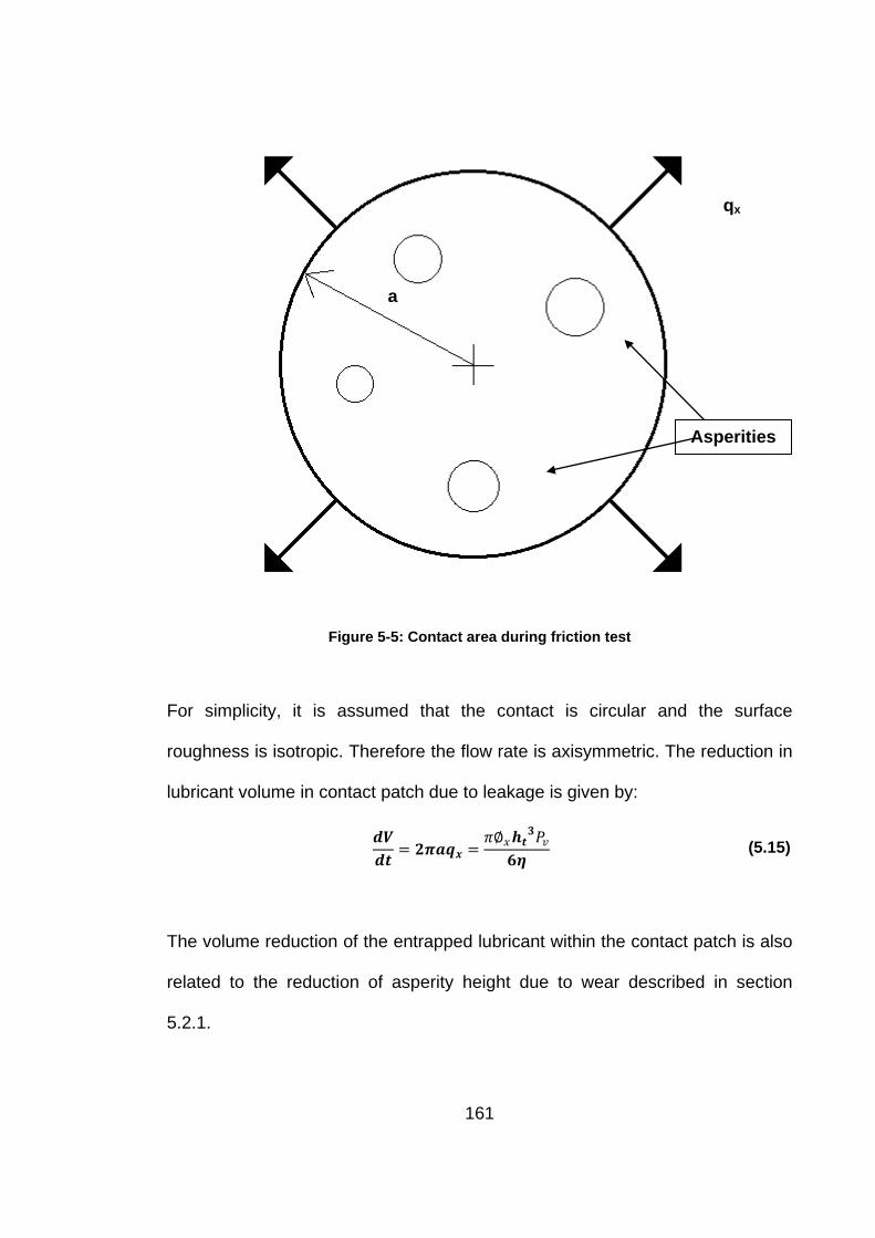
Figure 5-5: Contact area during friction test
For simplicity, it is assumed that the contact is circular and the surface
roughness is isotropic. Therefore the flow rate is axisymmetric. The reduction in
lubricant volume in contact patch due to leakage is given by:
𝒅𝒅𝑽𝑽𝒅𝒅𝑻𝑻
= 𝟐𝟐𝝅𝝅𝒂𝒂𝒒𝒒𝒙𝒙 =𝜋𝜋∅𝑥𝑥𝒉𝒉𝑻𝑻
𝟑𝟑𝑃𝑃𝑣𝑣𝟏𝟏𝟏𝟏
(5.15)
The volume reduction of the entrapped lubricant within the contact patch is also
related to the reduction of asperity height due to wear described in section
5.2.1.
a
qx
Asperities
161

𝒅𝒅𝑽𝑽𝒅𝒅𝑻𝑻
= 𝝅𝝅𝒂𝒂𝟐𝟐(𝟏𝟏 − 𝑨𝑨)𝒌𝒌𝟒𝟒𝒂𝒂𝑯𝑯𝒗𝒗 (5.16)
Therefore the pressure in the valleys can then be derived by combining Eq.
5.15 and 5.16 as:
𝟒𝟒𝒗𝒗 =𝟏𝟏𝟏𝟏𝒂𝒂𝟐𝟐 �𝒌𝒌 𝟒𝟒𝒂𝒂
𝑯𝑯𝒗𝒗� (𝟏𝟏 − 𝑨𝑨)
𝝓𝝓𝒙𝒙𝒉𝒉𝑻𝑻𝟑𝟑 (5.17)
As the sliding distance and wear area increases, the pressure in the valleys
becomes more prominent than in the initial cycles. The proprietary lubricant has
a viscosity of 50,000 cP (50 Pa.s). Solving Equations 5.3, 5.16 and 5.17
continuously with sliding distance will yield the variation of asperity height 𝒉𝒉,
asperity contact ratio 𝑨𝑨, valley pressure 𝟒𝟒𝒗𝒗and asperity contact pressure 𝟒𝟒𝒂𝒂.
Figure 5-6 shows the difference between the pressure on the asperities and the
pressure in the valleys for the first cycle of the friction test. The asperity
pressure is greatly more significant than the valley pressure at the first stroke
and becomes more prevalent in the second stroke as the contact ratio
increases.
Another consequence of wear is the reduction in asperity height and the
increase in the contact ratio with sliding distance. Figure 5-7 shows a
comparison between the sliding distance and the asperity height, and also the
contact ratio. This comparison is for the first cycle, showing both loading and
unloading. As the sliding distance increases, the asperity height reduces and as
the sliding distance increases the contact ratio, i.e. the area of contact between
the two surfaces, also increases.
162
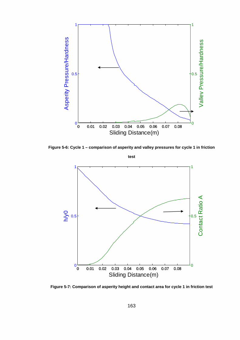
Figure 5-6: Cycle 1 – comparison of asperity and valley pressures for cycle 1 in friction
test
Figure 5-7: Comparison of asperity height and contact area for cycle 1 in friction test
0 0.01 0.02 0.03 0.04 0.05 0.06 0.07 0.080
0.5
1
Sliding Distance(m)
Asp
erity
Pre
ssur
e/H
ardn
ess
0 0.01 0.02 0.03 0.04 0.05 0.06 0.07 0.080
0.5
1
Val
ley
Pre
ssur
e/H
ardn
ess
0 0.01 0.02 0.03 0.04 0.05 0.06 0.07 0.080
0.5
1
h/y0
Sliding Distance(m)0 0.01 0.02 0.03 0.04 0.05 0.06 0.07 0.08
0
0.5
1
Con
tact
Rat
io A
163

Carbone et al (119) compared existing theories of contact between surfaces
and evaluated the differences in accuracy. The authors looked at theories from
the major contributors to contact theory and compared the advantages that
were given to the knowledge.
It is noted that hydrostatic pressure remains low until the asperity contact
percolation is reached which leads to rapid increase in lubricant pressure and
decrease in asperity pressure. Hence the wear of the asperity will diminish. The
percolation threshold depends on the Peklenik number. For a non-directional
surface, the Peklenik number is 1. The real surface can be described as
practically non-directional due to the spherical shape of the peened asperities
on the surface, however the plated surface has initial machine marks in
transverse to the sliding direction. Therefore the initial contact cannot be
described as non-directional. After the first stroke of sliding, galling marks will
be present on the plated surface. The surface will become more isotropic.
This allows for the prediction of the 𝑹𝑹𝒒𝒒 value for the shot peened surface. As
shown in Figure 5-8, the asperity wear diminishes after the first cycle so that
surface roughness stays constant. This is because the contact percolation is
reached and hence the valley pressure increases rapidly. This is in agreement
with the results taken from the samples after the first cycle but the discrepancy
increases after subsequent cycles. This indicates that the lubricant can still
escape after the percolation threshold is reached. It has been demonstrated
previously by Lo and Wilson (120) and Le et al (82) that lubricant can still be
drawn out of ‘micro-pools’ by relative sliding. Nevertheless, the current model
164

does capture the mechanism which leads to the main reduction of the surface
asperities. The focus is then switched to the study of the friction.
Figure 5-8: Effect of sliding distance on RMS roughness for surfaces with γ = 1
5.3 Friction model
As stated by Le et al (121), a correct value for CoF is vital in the estimation of
roll load and torque in rolling methods, however generally a constant value is
used. This is true for most OCTG pipe connections. The value is taken from a
set of API Standards and an accurate value is not predicted for each individual
condition of the connection. According to the API 7G Recommended Practice
(122), CoF between mating surfaces, i.e. threads and shoulders, is predicted to
be 0.07 - 0.08; this is true for thread compounds containing 40 – 60 wt% of
finely metallic zinc. However, there is no information in this standard which
0 0.05 0.1 0.15 0.2 0.25 0.30
0.5
1
1.5
2
2.5
3x 10
-6
Sliding Distance (m)
Rq
(m)
165
specifies the lubrication regime, contact pressure, sliding speed or surface
roughness of either of the two mating surfaces.
It is therefore inaccurate to presume that all surfaces would have the same
value of CoF associated with them. A new value is not calculated each time and
therefore it is not dependent on how many times the connection has been
made-up previously. This means that most likely, the value of torque calculated
from the CoF is not accurate. Although this may cause no difference to pipes in
some sections of the production string, the value could have catastrophic
problems in the future where the depth of the wells and the associated
temperature and pressure increase significantly. Although largely over-torqued
connections should be noticeable to the inspector, if the plastic deformation is
small, this can easily be missed.
A friction model was therefore produced to allow the calculation of the friction
coefficient with changes in surface roughness after testing. From the
experimental results it can be shown that as the sliding distance increases, the
surface roughness reduces to a certain point. The same occurs with the friction;
initially the surface roughness and friction are high but as the surface wears and
the roughness reduces, stabilise to a more constant value.
Identifying the main features on the surface is a useful technique to help
understand the structure of the surfaces in contact. The peened surface
typically has the largest value of roughness and therefore the source of the
value of CoF. It has been proven that for two surfaces of the same material, the
166

one with the highest roughness also has the highest CoF. From the SEM and
microscopic images, the surface features can be visually identified. It was the
work of Ahmed and Sutcliffe (68) that recognised the necessity for being able to
quantify these features. They produced a MATLAB code which was capable of
ascertaining which characteristics were peaks and which were troughs on the
material surface. Providing that the correct threshold values were supplied in
the code, algorithms were used to identify pits and roll marks in the surface.
This technique was modified to fit the surface characteristics of the samples
used in the current project to identify the pits on the peened surfaces. The area
fraction of pits was calculated for the initial shot peened sample and after each
test cycle. The results are shown in Figure 5-9. It is found that the size of the
pits decreases but the pit area ratio is approximately 0.50 even after the fourth
cycle. This means that the large pits are broken into small pits but the area ratio
remains more or less constant.
Figure 5-9: Ceramic peened sample pit percentage during friction/wear
0
10
20
30
40
50
60
70
0 1 2 3 4
Pit p
erce
ntag
e (%
)
Number of cycles
Ceramic peened sample pit percentage during friction/ wear testing
167

Similar to the work done by Sutcliffe et al (88), the steel material was shot
blasted with beads of a chosen material, resulting in the creation of pits on the
surface. Both are operated at low speed and in the boundary lubrication regime.
During the sliding of two surfaces in contact, the same motion experienced by
the connection during the make-up process, there is movement of the
lubricating film between the two surfaces. The difference however is that there
is bulk plastic deformation in the drawing process so that the asperity flattening
is different. To understand this movement and appreciate how it works, the
mechanism described in this paper was micro-plasto-hydrodynamic lubrication
(MPHL). MPHL is where the lubricant is drawn from the craters by relative
sliding due to the wedge effect while the surface is plastically stretched. This
process results in the creation of a very thin film with boundary additives on to
the asperity contacts.
Figure 5-10: Pit percentage comparison for each cycle
0
10
20
30
40
50
60
70
0 1 2 3 4
Pit p
erce
ntag
e (%
)
Number of cycles
Ceramic peened sample pit percentage during friction/ wear testing
168
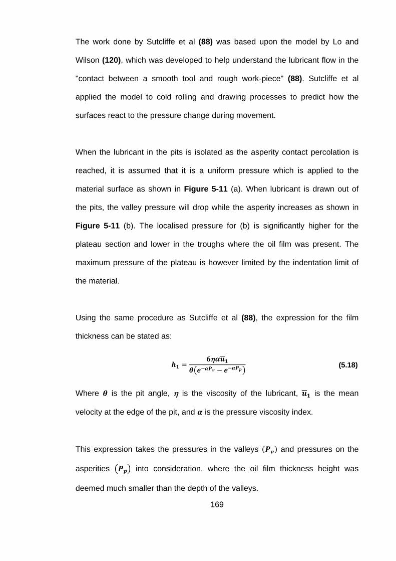
The work done by Sutcliffe et al (88) was based upon the model by Lo and
Wilson (120), which was developed to help understand the lubricant flow in the
"contact between a smooth tool and rough work-piece" (88). Sutcliffe et al
applied the model to cold rolling and drawing processes to predict how the
surfaces react to the pressure change during movement.
When the lubricant in the pits is isolated as the asperity contact percolation is
reached, it is assumed that it is a uniform pressure which is applied to the
material surface as shown in Figure 5-11 (a). When lubricant is drawn out of
the pits, the valley pressure will drop while the asperity increases as shown in
Figure 5-11 (b). The localised pressure for (b) is significantly higher for the
plateau section and lower in the troughs where the oil film was present. The
maximum pressure of the plateau is however limited by the indentation limit of
the material.
Using the same procedure as Sutcliffe et al (88), the expression for the film
thickness can be stated as:
𝒉𝒉𝟏𝟏 =𝟏𝟏η𝜶𝜶𝑫𝑫𝟏𝟏
𝜽𝜽�𝑻𝑻−𝜶𝜶𝟒𝟒𝒗𝒗 − 𝑻𝑻−𝜶𝜶𝟒𝟒𝒑𝒑� (5.18)
Where 𝜽𝜽 is the pit angle, η is the viscosity of the lubricant, 𝑫𝑫𝟏𝟏 is the mean
velocity at the edge of the pit, and 𝜶𝜶 is the pressure viscosity index.
This expression takes the pressures in the valleys (𝟒𝟒𝒗𝒗) and pressures on the
asperities �𝟒𝟒𝒑𝒑� into consideration, where the oil film thickness height was
deemed much smaller than the depth of the valleys.
169
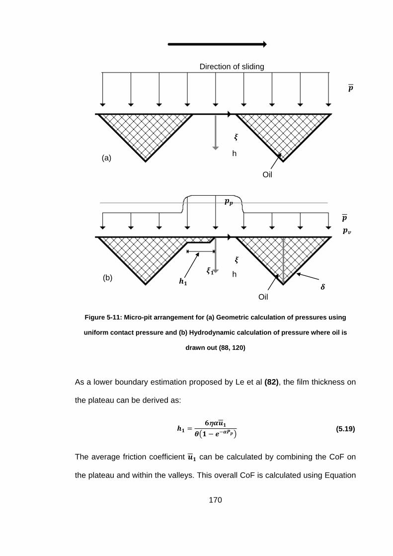
Figure 5-11: Micro-pit arrangement for (a) Geometric calculation of pressures using
uniform contact pressure and (b) Hydrodynamic calculation of pressure where oil is
drawn out (88, 120)
As a lower boundary estimation proposed by Le et al (82), the film thickness on
the plateau can be derived as:
𝒉𝒉𝟏𝟏 =𝟏𝟏η𝜶𝜶𝑫𝑫𝟏𝟏
𝜽𝜽�𝟏𝟏 − 𝑻𝑻−𝜶𝜶𝟒𝟒𝒑𝒑� (5.19)
The average friction coefficient 𝑫𝑫𝟏𝟏 can be calculated by combining the CoF on
the plateau and within the valleys. This overall CoF is calculated using Equation
Direction of sliding
h
h
𝒑𝒑
𝒑𝒑 𝒑𝒑𝒗𝒗
𝒑𝒑𝒑𝒑
𝜹𝜹
𝝃𝝃𝟏𝟏 𝝃𝝃
𝝃𝝃
Oil
Oil
𝒉𝒉𝟏𝟏
(a)
(b)
170
(5.20). This is done so by considering friction on the plateau. In this case, the
CoF on the valleys is significantly lower than that on the plateau and is therefore
regarded to as being negligible. Consequently, it is not included in this equation.
𝝁𝝁 = 𝑨𝑨𝒑𝒑𝝁𝝁𝒑𝒑 (5.20)
Where 𝑨𝑨𝒑𝒑 is the area ratio of the plateau and 𝝁𝝁𝒑𝒑 is the coefficient of friction on
the plateau.
Equation (5.21) is used to calculate the CoF on the plateau. This incorporates
the friction at the boundary contact 𝝁𝝁𝒃𝒃 with the friction coefficient of the lubricant
𝝁𝝁𝒗𝒗. Each is multiplied by the area ratio concerned with each section. 𝑨𝑨𝑭𝑭 is the
area ratio of the metal-to-metal contact and therefore (𝟏𝟏 − 𝑨𝑨𝑭𝑭) is the area ratio
of the thin film lubricant.
𝝁𝝁𝒑𝒑 = 𝑨𝑨𝑭𝑭𝝁𝝁𝒃𝒃 + (𝟏𝟏 − 𝑨𝑨𝑭𝑭)𝝁𝝁𝒗𝒗 (5.21)
The boundary friction coefficient 𝝁𝝁𝒃𝒃is regarded as a fitting parameter. 𝑨𝑨𝑭𝑭is
determined by the lubricant film thickness and the surface roughness on the
plateau which is given explicitly for each specific surface profile (123). The
friction coefficient of the lubricant thin film is calculated using Eyring’s equation.
𝝁𝝁𝒗𝒗 =𝝉𝝉𝟎𝟎𝒑𝒑�𝒔𝒔𝑻𝑻𝑻𝑻𝒉𝒉�
(𝟏𝟏𝒗𝒗)𝝉𝝉𝟎𝟎𝒉𝒉𝟏𝟏
� (5.22)
Where 𝝉𝝉𝟎𝟎 is the Erying shear stress of the lubricant, 𝒑𝒑� is the mean contact
pressure, 𝒉𝒉𝟏𝟏 is derived by Equation 5.19.
171

The parameters used in the calculation of the average CoF are summarised in
Table 5-2.
Table 5-2: Model parameters
Parameter Value
Contact Modulus, E* 113 GPa
Contact Radius, R* 60 mm
Vicker’s Hardness, H 2.6 GPa
Initial Surface Roughness of top sample, 𝑅𝑅𝑞𝑞 ,1 2.80 𝜇𝜇𝜇𝜇
Initial Surface Roughness to bottom sample , 𝑅𝑅𝑞𝑞 ,2 2.8 𝜇𝜇𝜇𝜇
Angle of Asperity, 𝜃𝜃 10°
Area ratio on the plateau, Ap 0.45
Wear Rate, 𝑘𝑘 3 x 10⁻⁴
Coefficient of Friction on the boundary layer, 𝜇𝜇𝑏𝑏 0.6
Eyring’s Shear Stress, 𝜏𝜏0 2 MPa
Viscosity, 𝜂𝜂 50 Pa.s
Viscosity pressure index, α 3.88 x 10⁻⁸ /Pa
In order to produce a model which was in line with the actual results obtained
during the physical testing, a number of assumptions had to be made. One
hypothesis was that the type of wear which occurred during the sliding was
somewhere between severe and mild wear. Therefore, as severe wear occurs
with a wear coefficient in the range of around 1x10⁻⁶ and mild wear at around
1x10⁻², using best fit parameters the wear coefficient used in the program was
3x10⁻⁴. The initial coefficient of friction predicted on the boundary layer was 0.6
as this was assumed to be metal-to-metal contact. The proprietary synthetic film
lubricant had a viscosity of 50 Pa.s which was obtained from the Data Sheet
provided by the manufacturer. In order to determine the Eyring shear stress
value, a lubricant with a similar viscosity was used as reference. The surface
roughness of the sample was measured using the techniques noted in Chapter
172
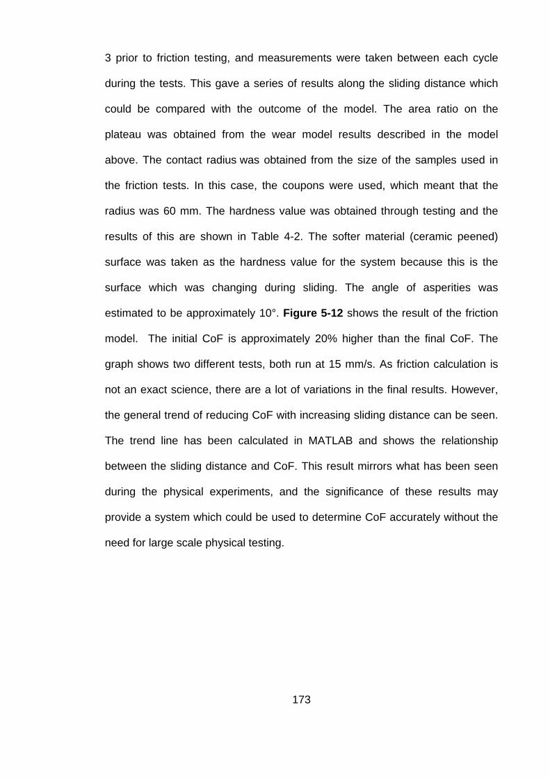
3 prior to friction testing, and measurements were taken between each cycle
during the tests. This gave a series of results along the sliding distance which
could be compared with the outcome of the model. The area ratio on the
plateau was obtained from the wear model results described in the model
above. The contact radius was obtained from the size of the samples used in
the friction tests. In this case, the coupons were used, which meant that the
radius was 60 mm. The hardness value was obtained through testing and the
results of this are shown in Table 4-2. The softer material (ceramic peened)
surface was taken as the hardness value for the system because this is the
surface which was changing during sliding. The angle of asperities was
estimated to be approximately 10°. Figure 5-12 shows the result of the friction
model. The initial CoF is approximately 20% higher than the final CoF. The
graph shows two different tests, both run at 15 mm/s. As friction calculation is
not an exact science, there are a lot of variations in the final results. However,
the general trend of reducing CoF with increasing sliding distance can be seen.
The trend line has been calculated in MATLAB and shows the relationship
between the sliding distance and CoF. This result mirrors what has been seen
during the physical experiments, and the significance of these results may
provide a system which could be used to determine CoF accurately without the
need for large scale physical testing.
173
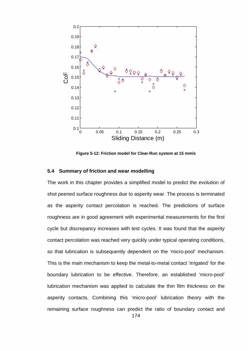
Figure 5-12: Friction model for Clear-Run system at 15 mm/s
5.4 Summary of friction and wear modelling
The work in this chapter provides a simplified model to predict the evolution of
shot peened surface roughness due to asperity wear. The process is terminated
as the asperity contact percolation is reached. The predictions of surface
roughness are in good agreement with experimental measurements for the first
cycle but discrepancy increases with test cycles. It was found that the asperity
contact percolation was reached very quickly under typical operating conditions,
so that lubrication is subsequently dependent on the ‘micro-pool’ mechanism.
This is the main mechanism to keep the metal-to-metal contact ‘irrigated’ for the
boundary lubrication to be effective. Therefore, an established ‘micro-pool’
lubrication mechanism was applied to calculate the thin film thickness on the
asperity contacts. Combining this ‘micro-pool’ lubrication theory with the
remaining surface roughness can predict the ratio of boundary contact and
0 0.05 0.1 0.15 0.2 0.25 0.30.1
0.11
0.12
0.13
0.14
0.15
0.16
0.17
0.18
0.19
0.2
Sliding Distance (m)
CoF
174

hence the average CoF. The CoF predictions are in line with experimental
measurements.
175

Chapter 6 : Discussion and Conclusions
Accurate calculation of friction is fundamental; it is, however, very complex and
any minor changes in external circumstances can have major consequences on
the final value of CoF. The subject of friction is not completely understood and
there is not a prescribed method of calculation for every type of material under
every condition available. This is because some theories work under certain
circumstances and others do not. The American Petroleum Institute (API) has a
standard value recommended for some of their procedures however its
accuracy is uncertain. The main issue with their calculation is that the same
value of CoF is used for every material type, without taking into consideration
the roughness of the surface, the speed at which it is made up or even the type
of materials that constitute the connection. This current value is satisfactory for
present conditions. However, since the torque value used to make-up
connections is highly dependent on this, there is the possibility for error. The
outcomes of this project conclude that through investigation of the materials that
form the manufacturer’s premium tubular connections, there are variations in
the final CoF. This was based on laboratory tests on different surface
roughness values and by varying the contact pressure experienced by the
materials, at the speeds associated with make-up.
Changes in all external conditions have the possibility to cause some effect on
CoF. The significance of this change is subject to how the changes affect the
lubrication between the two samples. The velocity of sliding, the type of
lubricant, the surface roughness, type of surface peening and contact pressure
176
all cause different reactions to CoF. The largest effect comes from the initial
surface roughness. The current procedure in the majority of the OCTG industry
is to make the connection up three times for casings, and ten times for tubing
before discarding the products. A value of torque is determined for each
connection using the friction values and the connection size; however CoF is
taken to be around 0.07-0.08 as standard. There is no consideration of changes
in the CoF used in the calculation of torque the second or third time the
connection has been made-up. The same torque value is reused each time.
The work in this project concludes that the surface roughness and CoF reduce
significantly after initial contact. This is caused by the flattening of asperities due
to wear. Chapter 5 details a method of predicting the surface roughness and
CoF during the make-up procedure. Such a model would improve connection
success rate, and could save the company significant money should leakages
or failures be caused by an insufficient seal between surfaces due to
inadequate or excessive make-up torque.
The details of the CoF test results are shown and analysed in Chapter 4. The
largest variations in the CoF are a result of the surface roughness. In the
majority of cases, samples of the same roughness(no matter what type of
media was used in peening) resulted in a similar CoF. Another typical
conclusion is that as the initial surface roughness increases, CoF also rises.
Regime 3 includes a smaller quantity of tests because the process was more
difficult and there was a significantly larger expense in producing the test
samples. This was beyond the scope of the HES project and budget. The new
testing rig, produced to undertake the Regime 3 tests, was less reliable than the
177
test rig used for the other two regimes. This was due to the size and material
required for manufacture. Although the values produced from the Regime 3
tests were of the magnitude expected, there was some uncertainty upon each
individual value. The very low pressures, however, are less significant as it was
the localised high stresses in the seal which were of main interest. It was not at
these magnitudes of pressure that failure could occur. As the localised contact
pressure between the samples used in the testing was significantly greater than
the yield stress of the materials, the higher pressures were more of a concern to
the industry. Nevertheless, the major subject of concern was in the differences
in CoF after wear of the initial surface. Due to the procedure used to make-up
the connection, and the fact that the torque applied to the connection was
calculated using CoF, significant differences between the CoF value in the initial
and final make-up cycles could have catastrophic consequences on the
connection functionality. As a minor leakage can cost the industry and
environment dearly, an investigation into the effect had to be done.
A simplified asperity flattening and friction model was presented in Chapter 5.
The model allowed for the prediction of burnishing of the shot peened surface
and the average CoF for the conditions of laboratory tests. Although the
hydrodynamic flow of lubricant was simplified significantly, the prediction of the
asperity flattening in the initial stage of sliding was in agreement with
experimental measurements. An established ‘micro-pool’ lubrication mechanism
was applied to estimate the ratio of asperity contact and the CoF. The results
are in concurrence with the laboratory test results.
178
Chapter 7 : Future Work
7.1 Oil Country Tubular Goods Industry Standards
Further improvements in the standardisation of CoF testing are needed in the
future to improve the accuracy of calculation of the torque used in make-up. The
current method of using an industry standard value of 0.07 to 0.08 potentially
has a degree of inaccuracy, and may cause problems with under or over-
torqued connections in the future. Although there is a large amount of research
being done into finding more sustainable ways of producing energy, the oil and
gas industry remains at the forefront of energy production worldwide. As the
sources are drained in the current wells, deeper drilling is required to keep up
with current demand. As the wells deepen, the pressures and temperatures that
the connections experience increase, and thus the connections need to be
more accurate.
A standardised method of obtaining the working CoF is necessary to ensure
that every OCTG connection producer uses the same technique. The American
Petroleum Institute (API) already has a substantial number of Standards and
Recommended Practices that each connection must satisfy in order to be
approved by a classification society. However, even though there are
recommendations about how this value should be obtained, there is no current
method in any of these standards which determines how every CoF value must
be attained. The costs associated with a proposal such as this are significantly,
high and would require solid justification to prove that it was deemed necessary.
The current project does show that the CoF changes with different external
179
circumstances, although in order to merit its significance, much larger scaled
projects need to be done to ensure that improvements are made in the future.
7.2 Temperature investigation
Although the project produced an extensive range of CoF data, and looked at a
wide variety of external circumstances, there was some additional work which
could have been done which would have added further value to the project.
Every CoF test was undertaken at room temperature (approximately 18 to
22ºC), as temperature was not one of the external circumstances in the initial
project scope. The temperature may have had an effect on CoF, but the
temperatures that the pipeline experiences in the field are much higher than
those which were used within this testing procedure. As the pipes and couplings
can be used in extremely hot and cold environments, further work could be
done in the future to allow a range of temperatures to be investigated.
The current test rig would not be sufficient to undertake such testing and any
improvements would have taken the project well beyond its scope and budget.
One method of obtaining results for changes in temperature would be to heat up
the samples in an oven (or cool them down by subjecting them to the solid form
of carbon dioxide known as dry ice),prior to being placed in the test rig ready for
the testing process to take place. The accuracy of such changes would be low
and the temperature changes of the samples would most likely change the
composition of the materials. The use of lubricants becomes another issue as
heating up or cooling down of the lubricants changes the viscosity and freezing
them would mean that they would not be able to be spread on the surface
180
easily. This is not comparable with what happens on the rig even with very low
temperatures so would not be equivalent. The case is similar to that of the
higher temperatures where most likely the lubricants would run off the surface
prior to contact. This would result in a number of extra tests being undertaken
with no improvements in results and the uncertainties of both the temperatures
and the behaviour of the lubrication would have reduced the reliability of the
project.
7.3 Development of the low pressure test
An enhanced testing process for the very low pressures would improve the
testing results, as a larger and more accurate set of results would be available.
A new load cell would have to be produced to improve the testing process.
Instead of using 2 mm strain gauges and gluing them to the legs of the load cell,
a much smaller set would be more accurate. This would have been a much
more complicated job to undertake and, if the wiring was not accurate enough,
would produce less reliable results. An alternative method would probably be
more precise, however this would seriously increase the costs and time
associated.
7.4 Helical motion
Although the complexity of producing such a test rig capable of helical motion is
high, the results may be improved if the sliding between the two contacting
surfaces was helical. The linear sliding motion used in this project was suitable
for understanding the effect of external conditions on CoF. However, if helical
motion was able to be replicated then the accuracy of the results would be
181

slightly higher. The cost and time associated in such a project was far beyond
the scope and budget of the project.
182

Chapter 8 : Appendices
Appendix 1: Sketches and Drawings of the Test rig
The top and bottom sample holders were manufacturered by the technical staff
of the University of Dundee and Plymouth University. These were made from an
aluminium alloy called Dural and held the samples in place allowing contact
during the testing process. Figure 8-1 shows the configuration for the large
pressure tests (Regime 1) carried out using the test rig. In this particular case,
the sample geometry was cylindrical, producing the largest contact pressure.
Figure 8-1: Test Rig Configuration
The test samples were produced using existing pipeline connections
manufactured by HES. These best represent the profiles of the contact surfaces
during make-up. A drawing of the coupon samples utilised in Regime 2 is
shown in Figure 8-2. Laser cutting was used to produce these samples. Figure
8-3 shows the pin samples used in Regime 2. These were turned on a milling
machine during manufacture.
183
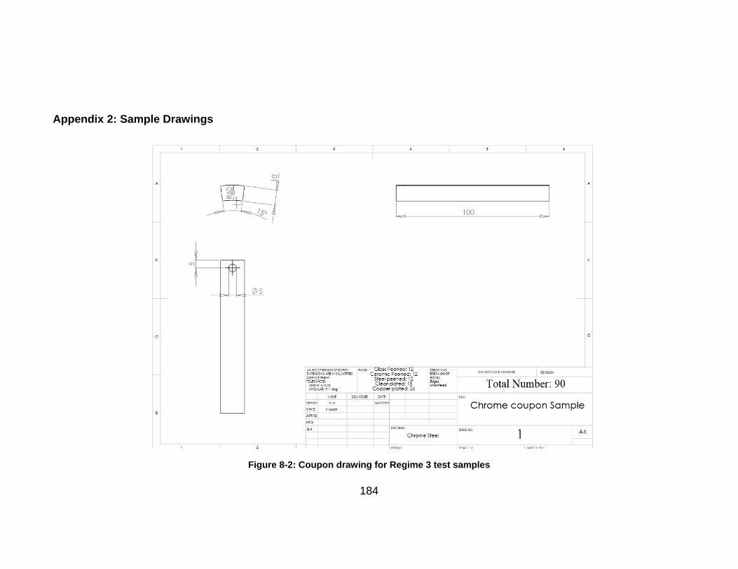
Appendix 2: Sample Drawings
Figure 8-2: Coupon drawing for Regime 3 test samples
184

Figure 8-3: Pin drawing for Regime 1 test samples
185

Appendix 3: Regime 3 Load Cell Drawings
Appendix 3 contains drawings for each of the components used in the Regime 1
and 2 set-ups. The assembly shown in Figure 8-4 shows the load cell which is
made up of a top plate [Figure 8-7], bottom plate [Figure 8-6] and legs (or rings)
[Figure 8-5].
Figure 8-4: Load cell assembly
186

Figure 8-5: Legs (rings) of Regime 1 and 2 load cell
187

Figure 8-6: Bottom plate of Regime 1 and 2 load cell
188
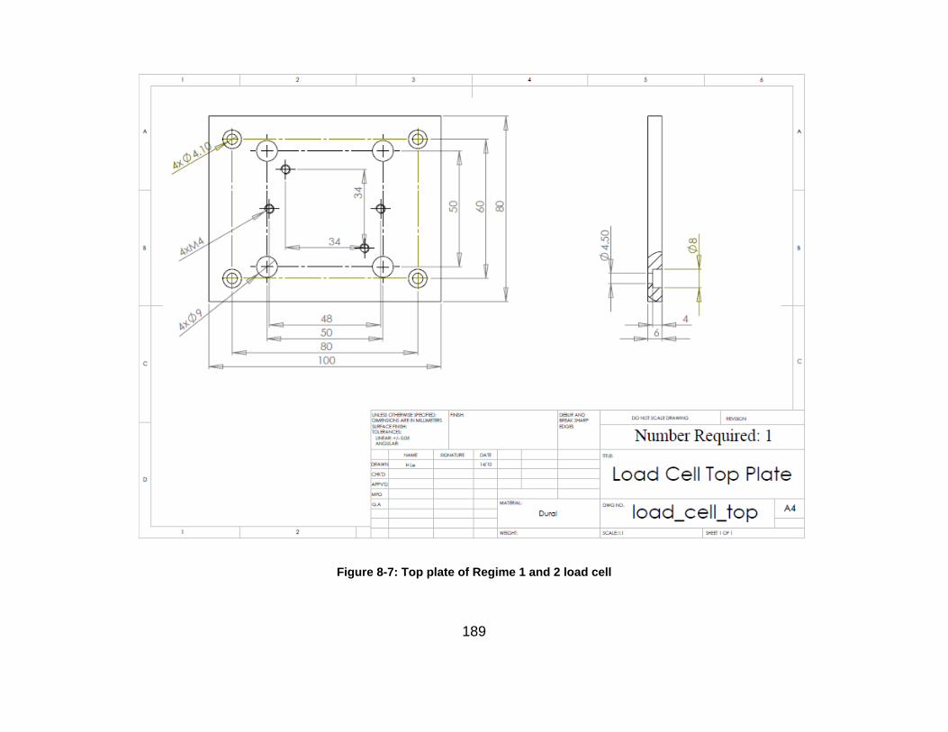
Figure 8-7: Top plate of Regime 1 and 2 load cell
189

The test rig is arranged as shown in Figure 8-8. There are two pole sections (shown in Figure 8-9 and Figure 8-10) which hold
the load cell, sample holders, motorised table and tilt table in place.
Figure 8-8: Load cell assembly
Top Sample
Load Cell
Tilt Table
Bottom Sample
Motorised Sliding Table
190
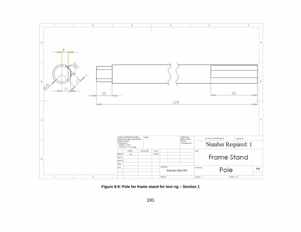
Figure 8-9: Pole for frame stand for test rig – Section 1
191

Figure 8-10: Pole for frame stand for test rig – Section 2
192
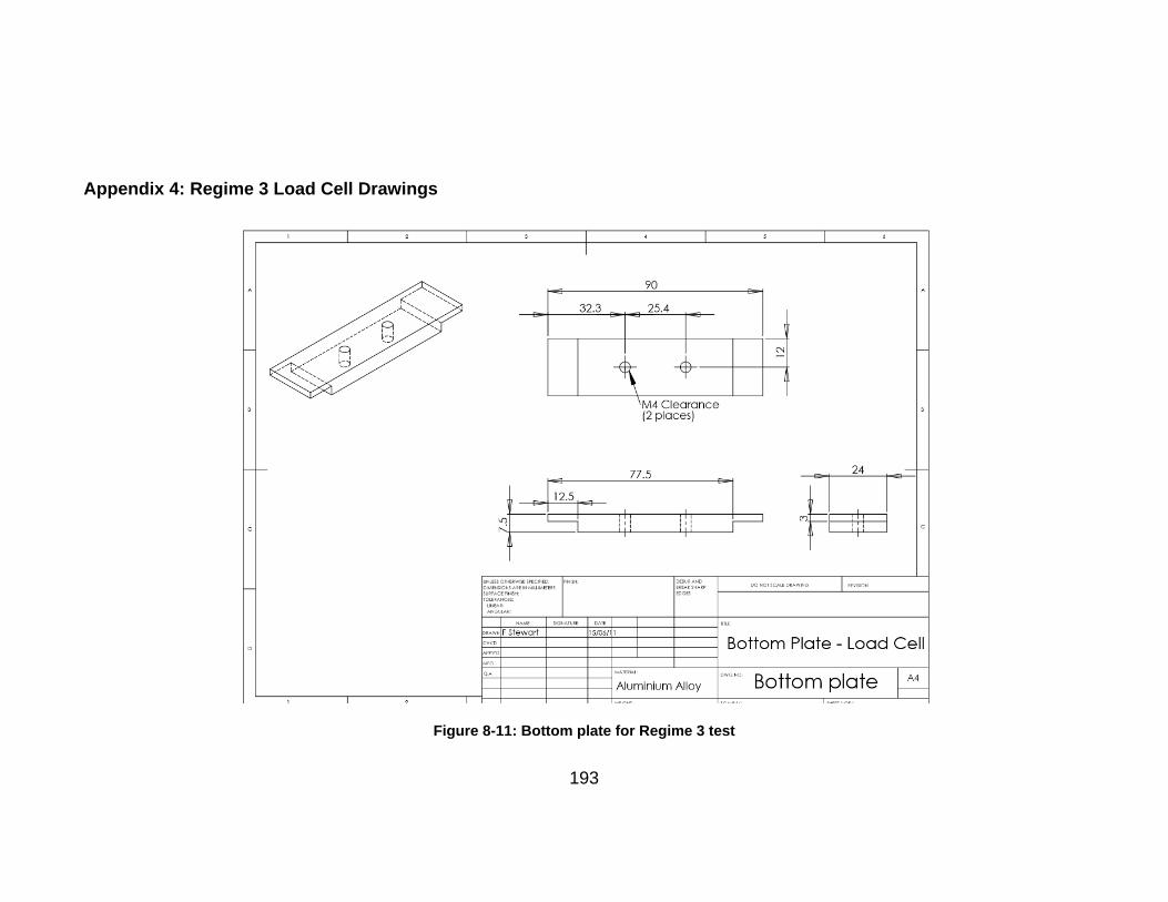
Appendix 4: Regime 3 Load Cell Drawings
Figure 8-11: Bottom plate for Regime 3 test
193

Figure 8-12: Top plate for Regime 3 test
194

Appendix5: Test Rig Operation Procedure
A test rig operating procedure is shown below.
• Turn on – Amplifiers, Motor, Computer
This takes approximately 30 minutes to warm-up properly to be ready to start.
1. Balance amplifiers
Place the samples into the test rig, securing them with the screws. Ensure that the samples are flat
in the sample holder. When there is no load applied on the test rig, zero the reading on the
oscilloscope. This is done by rotating the Position dials for both the Tangential and Normal Force
signals.
2. Apply a thin layer of lubricant to both samples
Use a high quality acrylic paint brush to prevent any bristles shedding onto the samples which will
affect the test. Each paintbrush is labelled for the individual lubricants. Ensure that these are used
only for the specified lubricant.
3. Adjust the tilt table
Using the spirit level, check that sample is horizontal, ensuring that the top plate parallel to the
table.
Check the samples are in contact with each other – by applying a minimum force (pressing down
with one finger) on the top sample and confirm that the oscilloscope moves approximately half a
division.
For the current assembly, a tilt of 12.8 gives 450 MPa (~ 8V). Before beginning experiments with an
alternative set-up, the amount of tilt needs to be established. Obtain this value by using small
Safety Note:
• Do not put fingers in contact area. • Do not stand too close to test rig.
195

running distances. i.e. the full distance along the sample is 45 mm, so initially tilt the micrometer a
limited amount e.g. moves it along 15mm to begin with, then increase until the user is fully confident
that the load cell will not be overloaded.
4. Apply lubricant and lower top sample.
Apply lubricant to the surface of the sample, ensure that it is thinly spread across the area of
contact during the test.
Check that the top sample is horizontal using the spirit level.
Check the samples are in contact – apply minimum force (by pressing down slightly) on the top
sample and check that the oscilloscope moves approximately half a division.
5. Tighten the locking nuts gently until the two samples are locked tightly together and cannot
move. Overdoing this can damage the load cell and not tightening it enough will give false
results.
6. Ensure nothing is obstructing the motorised table
7. Set-up an Aerotech program to complete the required number of cycles of linear travel at
the speeds desired (see later Appendix for programs)
8. In Labview, set up a program to record data from both the normal and tangential amplifiers
for the full length of the test, first click the Run button on the Labview Program to start the
recording.
The select the Save button
Run
196
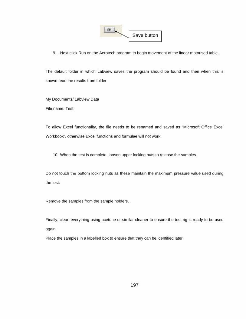
9. Next click Run on the Aerotech program to begin movement of the linear motorised table.
The default folder in which Labview saves the program should be found and then when this is
known read the results from folder
My Documents/ Labview Data
File name: Test
To allow Excel functionality, the file needs to be renamed and saved as “Microsoft Office Excel
Workbook”, otherwise Excel functions and formulae will not work.
10. When the test is complete, loosen upper locking nuts to release the samples.
Do not touch the bottom locking nuts as these maintain the maximum pressure value used during
the test.
Remove the samples from the sample holders.
Finally, clean everything using acetone or similar cleaner to ensure the test rig is ready to be used
again.
Place the samples in a labelled box to ensure that they can be identified later.
Save button
197

Appendix 6: Aerotech Program
Aerotech design and manufacture accurate motion control, positioning
tables/stages and positioning systems. Their software Soloist ID is a single axis
motion controller which is used to power the motorised table. Due to its
functionality, the power supply, amplifier and position controller are combined
within the one system. The linear speed of the motorised table can reach up to 100
mm/s. The three codes used to control the motion for the 3 mm/s, 15 mm/s and 50
mm/s test are based upon a 45 mm contact sample length and are shown below.
Appendix 6a
3 mm/s Aerotech Soloist program
SETPOSCMD 100 ; Start 100mm from home position
REPEAT 3 ; Repeat this 3 times
FREERUN F 3 ; Move from R to L at3mm/s (i.e. Velocity = 3 mm/s)
DWELL 15 ; Run for 15 s (45 mm)
FREERUN F 0 ; Velocity = 0 mm/s - Pause to change direction
DWELL 2 ; Pause for 2 s
FREERUN F -3 ; Move from L to R at 3mm/s (i.e. Velocity = -3 mm/s)
DWELL 15 ; Run for 15 s (45 mm)
FREERUN F 0 ; Velocity = 0 mm/s - Pause to change direction
DWELL 2 ; Pause for 2 seconds to repeat cycles or stop
ENDREPEAT ; End of repeating section
198

Appendix 6b
15 mm/s Aerotech Soloist program
SETPOSCMD 100 ; Start 100 mm from home position
REPEAT 3 ; Repeat this 3 times
FREERUN F 15 ; Move from R to L at 15mm/s (i.e. Velocity = 15 mm/s)
DWELL 3 ; Run for 3 s (45 mm)
FREERUN F 0 ; Velocity = 0mm/s - Pause to change direction
DWELL 3 ; Pause for 2 s
FREERUN F -15 ; Move from L to R at 15 mm/s (i.e. Velocity = -3 mm/s)
DWELL 3 ; Run for 3 s (45 mm)
FREERUN F 0 ; Velocity = 0 mm/s - Pause to change direction
DWELL 3 ; Pause for 2 seconds to repeat cycles or stop
ENDREPEAT ; End of repeating section
Appendix 6c
50 mm/s Aerotech Soloist program
SETPOSCMD 100 ; Start 100 mm from home position
REPEAT 3 ; Repeat this 3 times
FREERUN F 50 ; Move from R to L at 50 mm/s (i.e. Velocity = 50mm/s)
DWELL 0.9 ; Run for 0.9 s (45 mm)
FREERUN F 0 ; Velocity = 0 mm/s - Pause to change direction
DWELL 1 ; Pause for 2 s
FREERUN F -50 ; Move from L to R at 50 mm/s (i.e. Velocity = -50 mm/s)
DWELL 0.9 ; Run for 0.9 s (45 mm)
FREERUN F 0 ; Velocity = 0 mm/s - Pause to change direction
DWELL 5 ; Pause for 2 seconds to repeat cycles or stop
ENDREPEAT ; End of repeating section
199

Appendix 7: Matlab Programme
Matlab Programme – “Christensen”
%Main program -Christensen surface model and Archard wear, updated 30/12/2012 close all clear all global asptype global hmean0temp global y0friction asptype='christensen'; v1 = 0.29; % Poissons ratio of peened sample - chrome steel v2 = 0.29; % Poissons ratio of plated sample - chrome steel E1 = 2.05E11; % Young's modulus of peened sample - chrome steel E2 = 2.05E11; % Young's modulus of plated sample - chrome steel Estar = 1/(((1-v1^2)/E1)+((1-v2^2)/E2)); %plane stress modulus from the material properties of both substances= Rq0=2.767E-6*sqrt(2); %Combined surface roughness of two surfaces - From heightmatrixworkingchange.m file Rq=Rq0/sqrt(2); %Estimated plataeu surface roughness K=3e-4; %Change this to suit, start with 0.001 Hv=2.6E9; %Ceramic peened chrome steel hardness result from Birmingham theta=10*pi/180; % alpha=3.88e-8; % lambda=100e-6; % y0=6*Rq0; %Surface roughness amplitude Wm=500; %Maximum load at largest sliding distance - For coupons - between 65-80 ksi (448-551 MPa) R = 0.06; %1/R=1/R1+1/R2, R2=infinity because perpendicular, so R=R1 (R1=R2) - For coupons R=60mm (0.06m), For pins R=6mm (0.006m) gamma=3; %Peklenik number - for non-directional surface, gamma=1 a2 = 0.051375*(log(9*gamma)).^3-0.0071901*(log(9*gamma)).^4; %flow factor coefficient a3 = 1.0019-0.17927*log(gamma)+0.042583*(log(gamma)).^2-0.016417*log(gamma)^3;%flow factor coefficient Htc = 3*((1-((0.47476/gamma)+1).^(-0.25007)));%percolation threshold eta = 50; %Viscosity - For ClearGlide, eta =50 Pa.s from 50,000CP v=0.015; v0=0.015; %(m/s) - speed) rho=1160; % in kg/m^3 - As ClearGlide relative density from datasheetis 1.160 Pvtemp=0; dh=0; htemp=y0; %initial valley pressure, asperity height change, asperity height %Cycle 1 loading dS=0.001; %Change in sliding distance S = [0:dS:0.045]; %Sliding distance (m) for cycle 1 Aa=zeros(1,length(S)); %Asperity contact areas for i=1:length(S) W(i)=Wm*(S(i)/0.045)+10; %Load applied - increases as sliding distance increases Pbartemp=1/pi*(((16*W(i)*Estar.^2)/(9*R.^2)).^(1/3)); %Mean contact pressure [atemp,hmean,hvartemp]=aspparas(htemp,y0); %Contact area determined using "aspparas" program Patemp=(Pbartemp-Pvtemp*(1-atemp))/atemp; Patemp=min(Patemp,Hv); a=(3/4*W(i)*R/Estar)^(1/3); %Contact radius %a=0.5*a; Ht=hmean/Rq0; if Ht>Htc phix = (a2*(Ht-Htc).^2+a3*(Ht-Htc).^3)/Ht^3; Pvtemp = 6*eta*a*(1-atemp)*(a*dh/dS*v0)/(phix*(hmean).^3); else Pvtemp=Pbartemp; Patemp=0; end Pvtemp=max(Pvtemp,0); Pv(i)=Pvtemp; Pbar(i)=Pbartemp; Pa=min(Patemp,Hv); %Pa cannot be higher than the hardness of the material
200
Pa=max(Pa,0); dh=K*Pa*dS/(Hv); %wear depth Pabar(i)=Patemp; hvar(i)=hvartemp; htemp=htemp-dh; h1(i)=htemp; Aa(i)=atemp; end KPH=(K*Pabar)/Hv; Wh=S.*KPH; %Wear increment %Calculate Surface Roughness of plataeu (Rq) during cycle 1+ Rqtemp=sqrt(0.5*hvar); % Rq of each surface Rq1=Rqtemp; %Cycle 1 unloading S2=[0.045:dS:0.090]; for i=1:length(S2) W2(i)=(((0-Wm)/(0.09-0.045))*S(i))+510; %Load applied - increases as sliding distance increases vel2=v0; Pbartemp=1/pi*(((16*abs(W2(i))*Estar.^2)/(9*R.^2)).^(1/3)); %Mean pressure when L=a [atemp,hmean,hvartemp]=aspparas(htemp,y0); Patemp=(Pbartemp-Pvtemp*(1-atemp))/atemp; Patemp=min(Patemp,Hv); a=(3/4*W2(i)*R/Estar)^(1/3); %Change this ht=sqrt(hvartemp+0.25*y0^2); Ht=hmean/Rq; if Ht>Htc phix = (a2*(Ht-Htc).^2+a3*(Ht-Htc).^3)/Ht^3; Pvtemp = 6*eta*a*(1-atemp)*(a*dh/dS*vel2)/(phix*(hmean).^3); else Pvtemp=Pbartemp; Patemp=0; end Pvtemp=max(Pvtemp,0); Pv2(i)=Pvtemp; Pbar2(i)=Pbartemp; Pa=min(Patemp,Hv); %Pa cannot be higher than the hardness of the material Pa=max(Pa,0); dh=K*Pa*dS/(Hv); Pabar2(i)=Pa; hvar2(i)=hvartemp; htemp=htemp-dh; h2(i)=htemp; Aa2(i)=atemp; end %Calculate Surface Roughness of plataeu (Rq) during cycle 1- Rq2=sqrt(0.5*hvar2); %Calculate Wear Height KPH2=(K*Pabar2)/Hv; Wh2=S2.*KPH2; %Wear height %Cycle 2 loading S3=[0.090:dS:0.135]; for i=1:length(S3) vel3=v0; W3(i)=Wm*(S(i)/0.045)+10; %Load applied - increases as sliding distance increases Pbartemp=1/pi*(((16*abs(W3(i))*Estar.^2)/(9*R.^2)).^(1/3)); %Mean pressure when L=a
201

[atemp,hmean,hvartemp]=aspparas(htemp,y0); atemp=max(atemp,0.01); Patemp=(Pbartemp-Pvtemp*(1-atemp))/atemp; Patemp=min(Patemp,Hv); a=(3/4*W2(i)*R/Estar)^(1/3); %Change this ht=sqrt(hvartemp+0.25*y0^2); Ht=hmean/Rq; if Ht>Htc phix = (a2*(Ht-Htc).^2+a3*(Ht-Htc).^3)/Ht^3; Pvtemp = 6*eta*a*(1-atemp)*(a*dh/dS*vel3)/(phix*(hmean).^3); else Pvtemp=Pbartemp; Patemp=0; end Pvtemp=max(Pvtemp,0); Pv3(i)=Pvtemp; Pbar3(i)=Pbartemp; Pa=min(Patemp,Hv); %Pa cannot be higher than the hardness of the material Pa=max(Pa,0); dh=K*Pa*dS/(Hv); Pabar3(i)=Pa; hvar3(i)=hvartemp; htemp=htemp-dh; h3(i)=htemp; Aa3(i)=atemp; end %Calculate Surface Roughness of plataeu (Rq) during cycle 2+ Rq3=sqrt(0.5*hvar3); %Calculate Wear Height KPH3=(K*Pabar3)/Hv; Wh3=S3.*KPH3; %Wear heigh %Cycle 2 unloading S4=[0.135:dS:0.180]; for i=1:length(S4) W4(i)=(((0-Wm)/(0.09-0.045))*S(i))+510; %Load applied - increases as sliding distance increases Pbartemp=1/pi*(((16*abs(W4(i))*Estar.^2)/(9*R.^2)).^(1/3)); %Mean pressure when L=a vel4=v0; [atemp,hmean,hvartemp]=aspparas(htemp,y0); atemp=max(0.01,atemp);%Contact area determined using "aspparas" program Patemp=(Pbartemp-Pvtemp*(1-atemp))/atemp; Patemp=min(Patemp,Hv); a=(3/4*W2(i)*R/Estar)^(1/3); %Change this ht=sqrt(hmean^2+0.25*y0^2); Ht=hmean/Rq; if Ht>Htc phix = (a2*(Ht-Htc).^2+a3*(Ht-Htc).^3)/Ht^3; Pvtemp = 6*eta*a*(1-atemp)*(a*dh/dS*vel4)/(phix*(hmean).^3); else Pvtemp=Pbartemp; Patemp=0; end Pvtemp=max(Pvtemp,0); Pvtemp=min(Pvtemp, Pbartemp); Pv4(i)=Pvtemp; Pbar4(i)=Pbartemp; Pa=min(Patemp,Hv); Pa=max(Pa,0);%Pa cannot be higher than the hardness of the material dh=K*Pa*dS/(Hv); Pabar4(i)=Pa; hvar4(i)=hvartemp;
202

htemp=htemp-dh; h4(i)=htemp; Aa4(i)=atemp; end %Calculate Surface Roughness of plataeu (Rq) during cycle 2- Rq4=sqrt(0.5*hvar4); %Calculate Wear Height KPH4=(K*Pabar4)/Hv; Wh4=S4.*KPH4; %Wear heigh %Cycle 3 loading S5=[0.180:dS:0.225]; for i=1:length(S5) vel5=v0; W5(i)=Wm*(S(i)/0.045)+10; %Load applied - increases as sliding distance increases Pbartemp=1/pi*(((16*abs(W5(i))*Estar.^2)/(9*R.^2)).^(1/3)); %Mean pressure when L=a [atemp,hmean,hvartemp]=aspparas(htemp,y0); Patemp=(Pbartemp-Pvtemp*(1-atemp))/atemp; Patemp=min(Patemp,Hv); a=(3/4*W2(i)*R/Estar)^(1/3); %Change this ht=sqrt(hvartemp+0.25*y0^2); Ht=hmean/Rq; if Ht>Htc phix = (a2*(Ht-Htc).^2+a3*(Ht-Htc).^3)/Ht^3; Pvtemp = 6*eta*a*(1-atemp)*(a*dh/dS*vel4)/(phix*(hmean).^3); else Pvtemp=Pbartemp; Patemp=0; end Pvtemp=max(Pvtemp,0); Pv5(i)=Pvtemp; Pbar5(i)=Pbartemp; Pa=min(Patemp,Hv); Pa=max(Pa,0);%Pa cannot be higher than the hardness of the material dh=K*Pa*dS/(Hv); Pabar5(i)=Patemp; hvar5(i)=hvartemp; htemp=htemp-dh; h5(i)=htemp; Aa5(i)=atemp; end %Calculate Surface Roughness of plataeu (Rq) during cycle 3+ Rq5=sqrt(0.5*hvar5); %Calculate Wear Height KPH5=(K*Pabar5)/Hv; Wh5=S5.*KPH5; %Wear heigh %Cycle 3 unloading S6=[0.225:dS:0.270]; for i=1:length(S6) vel6=v0; W6(i)=(((0-Wm)/(0.09-0.045))*S(i))+510; %Load applied - increases as sliding distance increases Pbartemp=1/pi*(((16*abs(W6(i))*Estar.^2)/(9*R.^2)).^(1/3)); %Mean pressure when L=a [atemp,hmean,hvartemp]=aspparas(htemp,y0);
203
atemp=max(0.01,atemp);%Contact area determined using "aspparas" program Patemp=(Pbartemp-Pvtemp*(1-atemp))/atemp; Patemp=min(Patemp,Hv); a=(3/4*W2(i)*R/Estar)^(1/3); %Change this ht=sqrt(hvartemp+0.25*y0^2); Ht=hmean/Rq; if Ht>Htc phix = (a2*(Ht-Htc).^2+a3*(Ht-Htc).^3)/Ht^3; Pvtemp = 6*eta*a*(1-atemp)*(a*dh/dS*vel6)/(phix*(hmean).^3); else Pvtemp=Pbartemp; Patemp=0; end Pvtemp=max(Pvtemp,0); Pv6(i)=Pvtemp; Pbar6(i)=Pbartemp; Pa=min(Patemp,Hv); %Pa cannot be higher than the hardness of the material Pa=max(Pa,0); dh=K*Pa*dS/(Hv); Pabar6(i)=Patemp; hvar6(i)=hvartemp; htemp=htemp-dh; h6(i)=htemp; Aa6(i)=atemp; end %Calculate Surface Roughness of plataeu (Rq) during cycle 3- Rq6=sqrt(0.5*hvar6); %Calculate Wear Height KPH6=(K*Pabar6)/Hv; Wh6=S6.*KPH6; %Wear height %Plot the results %Show relationship between Sliding Distance and Wear Depth %Show relationship between Sliding Distance and Contact Pressure figure(1) set(1,'Position', [400 500 480 400]); plot(S,Pabar) hold all plot(S2,Pabar2) hold all plot(S3,Pabar3) hold all plot(S4,Pabar4) hold all plot(S5,Pabar5) hold all plot(S6,Pabar6) hold all xlabel('Sliding Distance (m)','FontSize',14); ylabel('Contact Pressure (Pa)','FontSize',14); %Show relationship between Sliding Distance and Mean Pressure on the plateau when L=a figure(2) set(2,'Position', [800 500 480 400]); plot(S,Pbar) hold all plot(S2,Pbar2) hold all plot(S3,Pbar3) hold all plot(S4,Pbar4) hold all plot(S5,Pbar5) hold all plot(S6,Pbar6)
204
hold all xlabel('Sliding Distance (m)','FontSize',14); ylabel('Pbar (Pa)','FontSize',14); %Show relationship between Sliding Distance and Contact Area using aspparas function figure(3) set(3,'Position', [1200 500 480 400]); plot(S,Aa) hold all plot(S2,Aa2) hold all plot(S3,Aa3) hold all plot(S4,Aa4) hold all plot(S5,Aa5) hold all plot(S6,Aa6) hold all xlabel('Sliding Distance (m)','FontSize',14); ylabel('Contact Area','FontSize',14); %Show relationship between Sliding Distance and Surface roughness on the plateau figure(4) set(4,'Position', [5 30 480 400]); plot(S,Rq1) hold all plot(S2,Rq2) hold all plot(S3,Rq3) hold all plot(S4,Rq4) hold all plot(S5,Rq5) hold all plot(S6,Rq6) hold all axis([0 0.3 0 3E-6]) %errorbar(0,2.767E-6,0.168E-6,'xr') %1 Cycle plot(0.09,0.974E-6,'bx') plot(0.09,0.988E-6,'bx') plot(0.09,0.994E-6,'bx') plot(0.09,1.004E-6,'bx') plot(0.09,1.079E-6,'bx') plot(0.09,0.911E-6,'bx') %2 Cycle plot(0.18,0.868E-6,'bx') plot(0.18,0.840E-6,'bx') plot(0.18,0.787E-6,'bx') plot(0.18,0.767E-6,'bx') plot(0.18,0.855E-6,'bx') plot(0.18,0.791E-6,'bx') %3 Cycle plot(0.27,0.736E-6,'bx') plot(0.27,0.658E-6,'bx') plot(0.27,0.663E-6,'bx') plot(0.27,0.713E-6,'bx') plot(0.27,0.705E-6,'bx') plot(0.27,0.667E-6,'bx') hold on %errorbar(0.090,0.992E-6,0.054E-6,'xr') %hold all %errorbar(0.180,0.818E-6,0.042E-6,'xr') %hold all
205
%errorbar(0.270,0.690E-6,0.032E-6,'xr') %hold all xlabel('Sliding Distance (m)','FontSize',14); ylabel('Rq (m)','FontSize',14); %Show relationship between Sliding Distance and Load Applied During Sliding figure(5) set(5,'Position', [400 30 480 400]); plot(S,W) hold all plot(S2,W2) hold all plot(S3,W3) hold all plot(S4,W4) hold all plot(S5,W5) hold all plot(S6,W6) hold all xlabel('Sliding Distance (m)','FontSize',14); ylabel('Load (N)','FontSize',14); axis([0 0.27 0 3E-6]) %Show relationship between Sliding Distance and Load Applied During Sliding figure(6) set(6,'Position', [800 30 480 400]); plot(S,h1) hold all plot(S2,h2) hold all plot(S3,h3) hold all plot(S4,h4) hold all plot(S5,h5) hold all plot(S6,h6) hold all xlabel('Sliding Distance(m)','FontSize',14); ylabel('Asperity height (m)','FontSize',14); %Show relationship between Sliding Distance and Pv figure(7) set(7,'Position', [0 30 480 400]); plot(S,Pv) hold all plot(S2,Pv2) hold all plot(S3,Pv3) hold all plot(S4,Pv4) hold all plot(S5,Pv5) hold all plot(S6,Pv6) hold all xlabel('Sliding Distance(m)','FontSize',14); ylabel('Asperity height (m)','FontSize',14); Pabarcycle1=[Pabar Pabar2]; Pvcycle1=[Pv Pv2]; SD=[S S2]; %Show relationship between Sliding Distance and Pv figure(8)
206
set(8,'Position', [0 30 480 400]); ax = plotyy(SD,(Pabarcycle1/Hv),SD,(Pvcycle1/Hv),'plot'); hold all set(ax, 'XLim', [0 0.09]) xlabel('Sliding Distance(m)','FontSize',14); set(ax, 'YLim', [0 1]) set(get(ax(1),'Ylabel'),'String','Asperity Pressure/Hardness','FontSize',14) set(get(ax(2),'Ylabel'),'String','Valley Pressure/Hardness','FontSize',14) set(ax(1),'YTick',[0:.5:1]) set(ax(2),'YTick',[0:.5:1]) hcycle1=[h1 h2]; Aacycle1=[Aa Aa2]; figure(9) set(9,'Position', [0 30 480 400]); axh = plotyy(SD,(hcycle1/y0),SD,(Aacycle1/atemp(1)),'plot'); set(axh, 'XLim', [0 0.09]) set(axh, 'YLim', [0 1]) set(get(axh(1),'Ylabel'),'String','h/y0','FontSize',14) set(get(axh(2),'Ylabel'),'String','Contact Ratio A','FontSize',14) axis([0,0.09,0,1]) set(axh(1),'YTick',[0:.5:1]) set(axh(2),'YTick',[0:.5:1]) xlabel('Sliding Distance(m)','FontSize',14); %Friction Model %This is fine after a certain sliding distance, however an initial friction %model is required for the first stroke. CoFb =0.6; % friction coefficient on metal-on-metal contact CoFv = 0.002; %Change this tau0=2e6; %Eyring shesr stress taua=0.2*Hv; Ap=0.45; % plateau area ratio outside the pits %Cycle 1+ for l=1:length(S); vel1=v0; hfriction=y0; y0friction=y0; hmphl=(6*eta*alpha*vel1)/(theta*(1-exp(-alpha*Hv))); hcen=2.8*(eta*vel1/Estar/R).^0.65*(W(l)/Estar/R^2)^(-0.21)*R; hmean0temp=hmphl; %[atempfriction, hmeanfriction, hvartempfriction] = aspparas(hmean0temp,y0friction); y0friction=6*sqrt(Rq1(l)^2+Rq^2);% asperity height on plateau hfric=fzero('hafunc2',0); [Ar, hmeanb, hvarb]=aspparas(hfric,y0friction); % hfric is the traugh height %Ar=min(Ar,Pbar(l)/Hv) temp=Ar; tau0=2e6; CoFv=tau0*asinh(eta*vel1/hmeanb/tau0)/Pbar(l); %Eyring model CoFv=min(CoFv,CoFb); CoFall(l)=Ap*(CoFb*Ar + CoFv*(1-Ar)); end %Cycle 1- for l=1:length(S); vel1=v0; hfriction=y0; y0friction=y0; hmphl=(6*eta*alpha*vel1)/(theta*(1-exp(-alpha*Hv))); hcen=2.8*(eta*vel1/Estar/R).^0.65*(W(l)/Estar/R^2)^(-0.21)*R; hmean0temp=hmphl; %[atempfriction, hmeanfriction, hvartempfriction] = aspparas(hmean0temp,y0friction); y0friction=6*sqrt(Rq2(l)^2+Rq^2); hfric2=fzero('hafunc2',0);
207
[Ar, hmeanb, hvarb]=aspparas(hfric2,y0friction); % hfric is the traugh height %Ar=min(Ar,Pbar(l)/Hv) temp(l)=Ar; tau0=2e6; CoFv=tau0*asinh(eta*vel1/hmeanb/tau0)/Pbar2(l); %Eyring model CoFv=min(CoFv,CoFb) CoFall2(l)=Ap*(CoFb*Ar + CoFv*(1-Ar)); end %Cycle 2+ for l=1:length(S); vel1=v0; hfriction=y0; y0friction=y0; hmphl=(6*eta*alpha*vel1)/(theta*(1-exp(-alpha*Hv))); hcen=2.8*(eta*vel1/Estar/R).^0.65*(W(l)/Estar/R^2)^(-0.21)*R; hmean0temp=hmphl; %[atempfriction, hmeanfriction, hvartempfriction] = aspparas(hmean0temp,y0friction); y0friction=6*sqrt(Rq3(l)^2+Rq^2); hfric3=fzero('hafunc2',0); [Ar, hmeanb, hvarb]=aspparas(hfric3,y0friction); % hfric is the traugh height %Ar=min(Ar,Pbar(l)/Hv) tau0=2e6; CoFv=tau0*asinh(eta*vel1/hmeanb/tau0)/Pbar3(l); %Eyring model CoFv=min(CoFv,CoFb); CoFall3(l)=Ap*(CoFb*Ar + CoFv*(1-Ar)); end %Cycle 2- for l=1:length(S); vel1=v0; hfriction=y0; y0friction=y0; hmphl=(6*eta*alpha*vel1)/(theta*(1-exp(-alpha*Hv))); hcen=2.8*(eta*vel1/Estar/R).^0.65*(W(l)/Estar/R^2)^(-0.21)*R; hmean0temp=hmphl; %[atempfriction, hmeanfriction, hvartempfriction] = aspparas(hmean0temp,y0friction); y0friction=6*sqrt(Rq4(l)^2+Rq^2); hfric4=fzero('hafunc2',0); [Ar, hmeanb, hvarb]=aspparas(hfric4,y0friction); % hfric is the traugh height %Ar=min(Ar,Pbar(l)/Hv) tau0=2e6; CoFv=tau0*asinh(eta*vel1/hmeanb/tau0)/Pbar4(l); %Eyring model CoFv=min(CoFv,CoFb); CoFall4(l)=Ap*(CoFb*Ar + CoFv*(1-Ar)); end %Cycle 3+ for l=1:length(S); vel1=v0; hfriction=y0; y0friction=y0; hmphl=(6*eta*alpha*vel1)/(theta*(1-exp(-alpha*Hv))); hcen=2.8*(eta*vel1/Estar/R).^0.65*(W(l)/Estar/R^2)^(-0.21)*R; hmean0temp=hmphl; %[atempfriction, hmeanfriction, hvartempfriction] = aspparas(hmean0temp,y0friction); y0friction=6*sqrt(Rq5(l)^2+Rq^2); hfric5=fzero('hafunc2',0); [Ar, hmeanb, hvarb]=aspparas(hfric5,y0friction); % hfric is the traugh height %Ar=min(Ar,Pbar(l)/Hv) tau0=2e6; CoFv=tau0*asinh(eta*vel1/hmeanb/tau0)/Pbar5(l); %Eyring model CoFv=min(CoFv,CoFb); CoFall5(l)=Ap*(CoFb*Ar + CoFv*(1-Ar)); end %Cycle 3- for l=1:length(S); vel1=v0;
208

hfriction=y0; y0friction=y0; hmphl=(6*eta*alpha*vel1)/(theta*(1-exp(-alpha*Hv))); hcen=2.8*(eta*vel1/Estar/R).^0.65*(W(l)/Estar/R^2)^(-0.21)*R; hmean0temp=hmphl; %[atempfriction, hmeanfriction, hvartempfriction] = aspparas(hmean0temp,y0friction); y0friction=6*sqrt(Rq6(l)^2+Rq^2); hfric6=fzero('hafunc2',0); [Ar, hmeanb, hvarb]=aspparas(hfric6,y0friction); % hfric is the traugh height %Ar=min(Ar,Pbar(l)/Hv) tau0=2e6; CoFv=tau0*asinh(eta*vel1/hmeanb/tau0)/Pbar6(l); %Eyring model CoFv=min(CoFv,0.1); CoFall6(l)=Ap*(CoFb*Ar + CoFv*(1-Ar)); end figure(12) set(12,'Position', [800 500 480 400]); plot(Pbar,CoFall) xlabel('Contact Pressure (Pa)','FontSize',14); ylabel('CoF','FontSize',14); hold on figure(13) set(13,'Position', [800 500 480 400]); plot(S,CoFall) axis([0 0.3 0.1 .2]) hold on plot(S2,CoFall2) plot(S3,CoFall3) plot(S4,CoFall4) plot(S5,CoFall5) plot(S6,CoFall6) xlabel('Sliding Distance (m)','FontSize',14); ylabel('CoF','FontSize',14); plot(0.001,0.174394,'bx') plot(0.01,0.1567286,'bx') plot(0.02,0.1646635,'bx') plot(0.03,0.1760868,'bx') plot(0.04,0.1794499,'bx') plot(0.05,0.1553237,'bx') plot(0.06,0.1585696,'bx') plot(0.07,0.1503934,'bx') plot(0.08,0.1535697,'bx') plot(0.09,0.1360539,'bx') plot(0.10,0.1481996,'bx') plot(0.11,0.1476034,'bx') plot(0.12,0.1576052,'bx') plot(0.13,0.1531775,'bx') plot(0.14,0.1533096,'bx') plot(0.15,0.1527194,'bx') plot(0.16,0.1449809,'bx') plot(0.17,0.1518542,'bx') plot(0.18,0.1361490,'bx') plot(0.19,0.1432556,'bx') plot(0.20,0.1489767,'bx') plot(0.21,0.1572341,'bx') plot(0.22,0.1520521,'bx') plot(0.23,0.1539898,'bx') plot(0.24,0.1523296,'bx') plot(0.25,0.1479000,'bx') plot(0.26,0.1523026,'bx') plot(0.27,0.1374660,'bx') plot(0.001,0.167287413,'rd')
209

plot(0.01,0.153870152,'rd') plot(0.02,0.162574223,'rd') plot(0.03,0.175694528,'rd') plot(0.04,0.180901916,'rd') plot(0.05,0.157059427,'rd') plot(0.06,0.159603631,'rd') plot(0.07,0.152118647,'rd') plot(0.08,0.154478661,'rd') plot(0.09,0.158215417,'rd') plot(0.10,0.144952667,'rd') plot(0.11,0.146642577,'rd') plot(0.12,0.155636185,'rd') plot(0.13,0.156082258,'rd') plot(0.14,0.15486357,'rd') plot(0.15,0.154213903,'rd') plot(0.16,0.148241825,'rd') plot(0.17,0.152666248,'rd') plot(0.18,0.147748683,'rd') plot(0.19,0.140042281,'rd') plot(0.20,0.147417524,'rd') plot(0.21,0.155760693,'rd') plot(0.22,0.151802958,'rd') plot(0.23,0.155593151,'rd') plot(0.24,0.154101166,'rd') plot(0.25,0.149883263,'rd') plot(0.26,0.153534956,'rd') plot(0.27,0.141938449,'rd') hold on Matlab program – “afunc” %program afunc.m to find area as a function of h/y0 % for triangular and christensen asperities function a=afunc(h,y0) %h is measured from bottom of the asperity to platen level %y0 is the total depth of the asperity %x is measured from original mean position %z is distance from mean position divided semi-height global asptype if(asptype(1:1)=='t') a=min(max(1-h./y0,0.),1.); else z=h*2 ./y0-1; z2=z.*z;z3=z2.*z;z4=z3.*z;z5=z4.*z;z6=z5.*z;z7=z6.*z;z8=z7.*z; a=(16-35*z+35*z3-21*z5+5*z7)/32; i=find(z>=1); %if(length(i)>=1) a(i)=zeros(size(i)); i=find(z<=-1); %if(length(i)>=1) a(i)=ones(size(i)); end %end Matlab Program – “Aspparas” %program aspparas.m to find asperity geometric parameters for triangular %and christensen asperities function [a ,hmean,hvar]=aspparas(h,y0) %a is the ratio of contact area %h is measured from bottom of the asperity to platen level %y0 is the total depth of the asperity assumed scalar here %x is measured from original mean position %z is distance from mean position/semi-height
210
%z=-1:0.001:1; %h and z are measured from mean postion %hmean is mean height over whole contact measured from platen %assume h isnt negative global asptype a=afunc(h,y0); %iap=find(h<=y0); ia0=find(h>y0); ia1=find(h<0); %easiest to do all the values, and then overwrite for the zero areas if asptype(1:1)=='t' %zmean measured from base, hmean from plateau zmean=y0/2*(1-a.*a); hmean=h-zmean; hvar=y0.*y0/12*(1-a).^3.*(1+3*a); %if(length(ia0)>=1) hvar(ia0)=y0.*y0/12*ones(size(ia0)); %end else %christensen %z ex ex2 are measured from mean of original surface %hmean from plateau %hvar is variance z=h*2 ./y0-1; z2=z.*z;z3=z2.*z;z4=z3.*z;z5=z4.*z;z6=z5.*z;z7=z6.*z;z8=z7.*z;z9=z8.*z; hmean=(y0/6)*3*(35+128*z+140*z2-70*z4+28*z6-5*z8)/256; ex2=(y0/6)*(y0/6)*(16+105*z3-189*z5+135*z7-35*z9)/32+(y0/6)*(y0/6)*9*z2.*a; ex=h-y0/2-hmean; hvar=ex2-ex.*ex; %if(length(ia0)>=1) %hmean(ia0)=h(ia0)-y0/2; hvar(ia0)=y0.*y0/36*ones(size(ia0)); %end end hmean(ia0)=h(ia0)-y0/2; hmean(ia1)=zeros(size(ia1)); hvar(ia1)=zeros(size(ia1));
211

References
1. Williams JA. Engineering Tribology. 2005 ed. Cambridge: Cambridge University Press; 2005. 488 p. 2. Abel P, Ferrante J. Modern Tribology Handbook, Volume One - Principles of Tribology: CRC Press; 2000. 3. Dowson D. History of Tribology. London: Longman Group Limited, 1979. 4. Ludema KC. Friction, lubrication, wear: textbook in tribology. Florida, USA: CRC Press; 1996. 257 p. 5. Arnell RDD, Peter; Halling, J; Whomes, Terence;. Tribology Principles and Design Applications. First Edition ed: Palgrave Macmillan; 1991. 6. Wilson WA. Word origins in science and technology: An etymological notebook Lexitheque Sudsexe; 1994. 586 p. 7. Rabinowicz E. Friction and wear of materials. 2nd Edition ed. New York, USA: John Wiley & Sons, Inc; 1995 1995. 315 p. 8. Vitintin JK, M; Dohda, K; Jahanmir, S;. Tribology of mechanical systems: A guide to present and future technologies. New York: ASME Press; 2004. 9. Beek Av. Tribology-ABC Delft, Netherlands2012 [26/03/2012]. Available from: http://www.tribology-abc.com/abc/history.htm. 10. Pugh B. A tribology text for students - friction and wear. London, UK: Butterworth & Co Ltd; 1973. 206 p. 11. Bowden FP, Tabor D. Friction: an introduction to tribology. Guildford, UK: Biddles Ltd; 1974. 178 p. 12. O'Connor JJR, E.F;. The MacTutor History of Mathematics archive St Andrews, UK2012 [28/03/12]. 13. Halling J, Nuri KA, Teer DG, Howarth RB, Whomes TL, Davies PB. Principles of Tribology. London, UK: The Macmillan Press Ltd.; 1978. 401 p. 14. Bush AW, Gibson RD. The elastic contact of a rough surface. Journal of Wear. 1975;35:87-111. 15. Hertz H. Uber die Beruhrung fester elastischer Korper (On the contact of elastic solids). Journal für die reine und angewandte Mathematik. 1882;92:156-71. 16. Wisniak J. Guillaume Amontons. Revista CENIC Ciencias Quimicas [CENIC Journal Science & Chemistry]. 2005;36(3):187-95. 17. Bowden FP, Tabor D. The Friction of Lubrication of Solids: Part II. London, UK: Oxford University Press; 1964. 544 p. 18. Press OU. Oxford Online Dictionary Oxford, UK: Oxford University Press; 2011 [cited 2011 05/12/11]. 19. Davis JR. ASM Materials Engineering Dictionary. 5th Edition ed. USA: ASM International; 2006. 20. Plint G, editor Tribology Testing. Cambridge Tribology Course; 2010; Cambridge, UK. 21. Plc H. Hunting Energy Services: Hunting Plc; 2013. Available from: http://www.huntingplc.com/. 22. Chapman RE. Petroleum Geology: Elsevier Science Publishers B,V; 1983.
212

23. Bellarby J. Well Completion Design. Elsevier, editor. Amsterdam, The Netherlands: Elsevier; 2009. 24. Perrin D. Well Completion and Servicing. petrole Ifd, editor. Rueil-Malmaison, France1999. 25. Macini P. Encyclopedia of Hydrocarbons. Italy: Treccani.IT; 2008. 26. Steel J. JFE Bear data sheet Handa, Japan: JFE Steel; 2013. 27. Guangjie Y, Zhenqiang Y, Qinghua W, Zhentong T. Numerical and experimental distribution of temperature and stress fields in API round threaded connection. Engineering Failure Analysis. 2006;13:1275-84. 28. Kent S, Amiel G, Faucon B. North Sea Gas Leak Could Cost Billions. The Wall Street Journal. 2012. 29. Gosden E. Total's Elgin gas leak costing $2.5m a day. The Telegraph. 2012. 30. Duggan TV. Applied engineering design and analysis. 1st Edition ed. London: Iliffe; 1969. 391 p. 31. Institute AP. API Test 5A3 3rd Edition; Recommended Practice on Thread Compounds for Casing, Tubing, Line Pipe, and Drill Stem; API Standards Catalogue. Englewood, Colorado, USA: American Petroleum Institute; 2010. p. 210. 32. Bezensek B. Finite Element Analysis of the Seal During Make-up. 2010. 33. Bengisu MT, Akay A. Stick-slip oscillations: Dynamics of friction and surface roughness. Journal of the Acoustical Society of America. 1998;105(1):195-204. 34. Coulomb CA. Memoires de Mathematique et de Physique de l'Academie Royale des Sciences: Theorie des machines simples. Paris: Academie Royale des Sciences, 1785. 35. Ford IJ. Roughness effect on friction for multi-asperity contact between surfaces. Journal of Physics D: Applied Physics. 1993;26:2219-25. 36. Nayak PR. Random process model of rough surfaces. Journal of Wear. 1973;26(3):305-33. 37. Menezes PL, Kishore, Kailas SV. Influence of roughness parameters on coefficient of friction under lubricated conditions. Sadhana. 2008;33(3):181-90. 38. Sedlacek M, Podgornik B, Vizintin J. Influence of surface preparation on roughness parameters, friction and wear. Journal of Wear. 2009;266:482-7. 39. Bradley AB, Nagasaku S, Verger E. Premium Connection Design, Testing and Installation for HPHT Sour Wells. SPE High Pressure-High Temperature Sour Well Design Applied Technology Workshop; 17-19 May; The Woodlands, Texas, USA2005. p. 1-8. 40. Standardisation IOf. ISO 13679. Petroleum and natural gas industries - Procedures for testing casing and tubing connections: ISO; 2002. 41. Schwind B. Mobil qualifies three tubling.casing connection product lines. Hart's Petroleum Engineer International. 1998:59-62. 42. Baragetti S, Clerici P, Matteazzi S. Friction and tightening force of conical threaded connections: experiments in various conditions. Int J Mater Prod Tec. 2003;19(5):414-30. 43. Van Wittenberghe J, De Pauw J, De Baets P, De Waele W, Wahab MA, De Roeck G. Experimental determination of the fatigue life of modified threaded pipe couplings. Procedia Engineer. 2010;2(1):1849-58. 44. De Baere I. Design of a three- and four-point bending setup for fatigue testing of fibre-reinforced thermoplastics.
213

45. Meng Q, Gao L, Liu F, Yang P, Fisher J, Jin Z. Contact mechanics and elastohydrodynamic lubrication in a novel metal-on-metal hip implant with an aspherical bearing surface. Journal of Biomechanics. 2010;43(849-857). 46. Shafiei M, Alpas AT. Effect of sliding speed on friction and wear behaviour of nanocrystalline nickel tested in an argon atmosphere. Journal of Wear. 2008;265:429-38. 47. Farhat ZN, Ding Y, Northwood DO, Alpas AT. Effect of grain size on friction and wear of nanocrystalline aluminium. Materials Science and Engineering. 1996;A206:302-13. 48. Kato K. Wear in relation to friction - a review. Journal of Wear. 2000;241:151-7. 49. Leslie J. An experimental inquiry into the nature and propagation of Heat. London1804. 562 p. 50. Greenwood JA, Williamson JBP. Contact of Nominally Flat Surfaces. Proceedings of The Royal Society of Mathematical, Physical and Engineering Sciences. 1966;295:300-19. 51. Johnson KL. Contact mechanics. Cambridge Cambridgeshire ; New York: Cambridge University Press; 1985. xi, 452 p. p. 52. Jackson RL, Green I. On the modeling of elastic contact between rough surfaces. Tribology Transactions. 2011;54:300-14. 53. Zavarise G, Borri-Brunetto M, Paggi M. On the resolution dependence of micromechanical contact models. Journal of Wear. 2007;262:42-54. 54. Carbone G. A slightly corrected Greenwood and Williamson model predicts asymptotic linearity between contact area and load. Journal of the Mechanics and Physics of Solids. 2009;57:1093-102. 55. Greenwood JA. A simplified elliptic model of rough surface contact. Journal of Wear. 2006;261:191-200. 56. Buczkowski R, Kleiber M. Elasto-plastic statistical model of strongly anisotropic rough surfaces for finite element 3D-contact analysis. Journal of Computer Methods in Applied Mechancs and Engineering. 2006;195:5141-61. 57. Kim H, Kardes N. Friction and lubrication. In: Altan T, Tekkaya AE, editors. Sheet Metal Forming - Fundamentals: ASM International; 2012. 58. Hironaka S. Boundary Lubrication and Lubricants. Three Bond: Technical News. 1984. 59. Singer IL, Pollock HM. Fundamentals of Friction: Macroscopic and Microscopic Processes. Netherlands: Kluwer Academic Publishers; 1992. 60. Qasim SA, Gulzar M, Malik MA. Influence of surface roughness factor in modeling isothermal piston skirts lubrication in initial engine start up. World Congress on Engineering2012. 61. Teodoriu C, McDonald H, Bollfrass C. Friction considerations in rotary shouldered threaded connections. 26th International Conference on Offshore Mechanics and Arctic Engineering; San Diego, California, USA: ASME; 2007. 62. Farr AP, editor Torque Requirements For Rotary Shouldered Connections And Selection of Connections For Drill Collars. ASME Petroleum Mechanical Engineering Conference; 1957; Tulsa, Oklahoma, USA: ASME Petroleum Division. 63. Jeng Y-R. Experimental study on the effects of surface roughness on friction. 35th STLE/ASME tribology conference; Fort Lauderdale, Florida, USA: STLE/ASME; 1989.
214
64. Qiao H-B. A study on friction and wear characteristics of nanometer Al2O3/PEEK composites under the dry sliding condition. Journal of Tribology International. 2006;40:105-10. 65. Burton RA. Effects of two-dimensional, sinusoidal roughness on the load support characteristics of a lubricant film. Journal of Basic Engineering. 1963;85(2):258-62. 66. Kudenatti RB, Basti DP, Bujurke NM. Numerical solution of the MHD Reynolds equation for squeeze film lubrication between two parallel surfaces. Applied Mathematics and Computation. 2012;218:9372-82. 67. Christensen H. The Oil Film in a Closing Gap. Proceedings of the Royal Society of London. 1962;266. 68. Ahmed R, Sutcliffe MPF. Identification of surface features on cold-rolled stainless steel strip. Journal of Wear. 2000;244:60-70. 69. Blencoe KA, Williams JA. The friction of sliding surfaces carrying boundary layers. Tribol Lett. 1997;3(1):121-3. 70. Blencoe KA, Williams JA. Friction of sliding surfaces carrying boundary films. Wear. 1997;203:722-9. 71. Georges JM, Mazuyer D, Tonck A, Loubet JL. Lubrication with a Thin Colloidal Layer. J Phys-Condens Mat. 1990;2:Sa399-Sa403. 72. Georges JM, Mazuyer D. Pressure Effects on the Shearing of a Colloidal Thin-Film. J Phys-Condens Mat. 1991;3(47):9545-50. 73. Le HR, Sutcliffe MPF, Williams JA. Friction and material transfer in micro-scale sliding contact between aluminium alloy and steel. Tribol Lett. 2005;18(1):99-104. 74. Blencoe KA, Roper GW, Williams J. The influence of lubricant rheology and surface topography in modelling friction at concentrated contacts. P I Mech Eng J-J Eng. 1998;212(J6):391-400. 75. Kapoor A, Williams JA, Johnson KL. The Steady-State Sliding of Rough Surfaces. Wear. 1994;175(1-2):81-92. 76. Sacher A. Slip Resistance and the James Machine 0.5 Static Coefficient of Friction- Sine Qua Non*. ASTM Standardization News. 1993:53. 77. Melhuish D, Wegand J. Coefficient of friction, the development of a standard portable device for the US Naval Fleet. Tri-Service Corrosion Conference; Springfield, Virginia, USA2007. 78. Khan ZA, Hadefield M, Wang Y. Pressurised chamber design for conducting rolling contact experiments with liquid refrigerant lubrication. Materials and Design. 2005;26(8):680-9. 79. Williams JA. Engineering tribology. New York: Cambridge University Press; 2005. xix, 488 p. p. 80. Podgornik B, Hogmark S, Pezdirnik J. Comparison between different test methods for evaluation of galling properties of surface engineered tool surfaces. Wear. 2004;257(7-8):843-51. 81. Imperial Scientific Industries. Pin on Disc Testers [Webpage]. http://www.tribotesters.com/pin_on_disc.htm; 2011 [cited 2011 20/8/2011]. Available from: http://www.tribotesters.com/pin_on_disc.htm. 82. Stewart F, Le HR, Williams JA, Leech A, Bezensek B, Roberts A. Characterisation of friction and lubrication regimes in premium tubular connections. Tribology International. 2012;53:159 - 66.
215

83. Carper HJ, Ertas A, Issa J, Cuvalci O. Effect of Some Material, Manufacturing, and Operating Variables on the Friction Coefficient in Octg Connections. J Tribol-T Asme. 1992;114(4):698-705. 84. Le HR, Williams JA, Luo JK. Characterisation of tribological behaviour of silicon and ceramic coatings under repeated sliding at micro-scale. Int J Surf Sci Eng. 2008;2(1-2):1-13. 85. Higounenc O. Correlation of shot peening parameters to surface characteristic. 9th International Conference and Exhibition on Shot Peening; Paris, France: Institute for Industrial Technology Transfer; 2005. p. 28-35. 86. Amaral R, Chong LH. Surface Roughness. 2002. 87. Mylonas GI, Labeas G. Numerical modelling of shot peening process and corresponding products: Residual stress, surface roughness and cold work prediction. Journal of Surface & Coatings Technology. 2011;205(19):4480-94. 88. Sutcliffe MPF, Le HR, Ahmed R. Modeling of micro-pit evolution in rolling or strip-drawing. Journal of Tribology. 2001;123:33-40. 89. Inc. VI. Surface Measurement Parameters for Wyko Optical Profilers. In: Inc. VI, editor. Tucson, Arizona: Veeco Instruments Inc.; 2002. 90. Research W. Wolfram Mathworld - Kurtosis: Eric Weisstein; 2013 [08/01/2013]. Available from: http://mathworld.wolfram.com/Kurtosis.html. 91. DeCarlo LT. On the meaning and use of Kurtosis. Journal of Psychological Methods. 1997;2(3):292-307. 92. Mate C, M. Tribology on the Small Scale -A Bottom Up Approach to Friction, Lubrication, and Wear. Oxford: Oxford University Press; 2008. 93. Rugar D, Hansma P. Atomic Force Microscopy. Physics Today. 1990;43(10):23-30. 94. Kossek S, Flowers M. Scanning Tunneling Microscopy Phoenix, Arizona, USA: Nanoscience Instruments Inc.; 2011. Available from: http://www.nanoscience.com/education/STM.html. 95. Meyer E. Atomic Force Microscopy. Journal of Progress in Surface Science. 1992;41:3-41. 96. Binnig G, Quate CF. Atomic Force Microscope. Physical Review Letters. 1986;56(9):930-4. 97. Facility AMMR. Sydney, Australia: Australian Learning and Teaching Council; 2011 [17/01/2013]. Available from: http://www.ammrf.org.au/myscope/confocal/confocal/. 98. Compact Oxford Dictionary Thesaurus, and Wordpower Guide. New York, USA: Oxford University Press Inc.; 2001. Oxford Dictionary. 99. OLS3000 OL-. LEXT Confocal Scanning Laser Microscope Manual. Japan: Olympus; 2008. 100. Swapp S. Scanning Electron Microscopy (SEM) Northfield, Minesota, USA: Carleton College; [18/01/2013]. Available from: http://serc.carleton.edu/research_education/geochemsheets/techniques/SEM.html. 101. Schweitzer J. Scanning Electron Microscope West Lafayette, Indiana, USA: Purdue University; 2012 [cited 2013 22/01/2013]. Available from: http://www.purdue.edu/rem/rs/sem.htm. 102. Kirk D. Residual stresses in shot peened components. The Shot Peener magazine. 2004.
216

103. ZirPro S-G. ZIRBLAST Safety Data Sheet No. DS MS BE 11 GB. In: S.E.P.R. SEdPR, editor. ZIRBLAST Shot Peening Media. Cedex France: Saint-Gobain ZirPro; 2001. p. 2. 104. Bowen J. Micro-hardness Measurements. 2012. 105. Al-Samarai RA, Haftirman, Ahmad KR, Al-Douri Y. Effect of Load and Sliding Speed on Wear and Friction of Aluminum – Silicon Casting Alloy<div data-canvas-width="8.85720006108284" data-font-name="Times New Roman" dir="ltr" style="font-size: 35.4288px; font-family: sans-serif; left: 746.683px; top: 139.037px; transform: scale(0.88572, 1); transform-origin: 0% 0% 0px;">. International Journal of Scientific and Research Publications. 2012;2(3):1-4. 106. Leech A. Discussion on maximum pressures in premium tubular connections. In: Stewart F, editor. 2013. 107. Institute AP. APi Spec 5L - Specification for Line Pipe. American Petroleum Institute; 2000. 108. Inc. MIC. Shot Peening Applications. Metal Improvement Company Inc.; 2001. 109. Zwörner O, Hölscher H, Schwarz UD, Wiesendanger R. The velocity dependence of frictional forces in point-contact friction. Journal of Applied Physics A: Materials Science & Processing. 1998;66(S1):263-7. 110. Wang Q, Zhou F, Chen K, Wang M, Qian T. Friction and wear properties of TiCN coatings sliding against SiC and steel balls in air and water. Journal of Thin Solid Films. 2011;519:4830-41. 111. Le HR, Sutcliffe MPF. A friction model for cold strip rolling with two-wavelength surface roughness in the "mixed" lubrication regime. Journal of Tribology. 2003;125:670-7. 112. MathWorks. MathWorks - MATLAB Overview Natick, Massachusetts, U.S.A.: MathWorks; 2013 [cited 2013 11/01/2013]. Available from: http://www.mathworks.co.uk/products/matlab/. 113. Kwon DH, Park ES, Huh MY, Kim HJ, Cae JC. Wear behaviour of Fe-based bult metallic glass composites. Journal of Alloys and Compounds. 2011;509(1):105-8. 114. Christensen H. Stochastic model for hydrodynamic lubrication of rough surfaces. Proceedings of the Institution of Mechanical Engineers. 1969-1970;184:1013-25. 115. Persson BNJ. Elastoplastic Contact between Randomly Rough Surfaces. Physical Review Letters. 2001;87(11):116101-1 - -4. 116. Patir N, Cheng HS. Average Flow Model for Determining Effects of 3-Dimensional Roughness on Partial Hydrodynamic Lubrication. J Lubric Tech-T Asme. 1978;100(1):12-7. 117. Li W-L, Chein W-T. Parameters for Roughness Pattern and Directionality. Tribol Lett. 2004;17(3):547-51. 118. Hamrock BJ, Dowson D. Elastohydrodynamic Lubrication of Elliptical Contacts for Materials of Low Elastic-Modulus I - Fully Flooded Conjunction. J Lubric Tech-T Asme.100(2): 236-45 1978. 119. Carbone G, Bottiglione F. Asperity contact theories: Do they predict linearity between contact area and load? Journal of Mechanics and Physics of Solids. 2008;56:2555-72. 120. Lo SW, Wilson WRD. A theoretical model of micro-pool lubrication in metal forming. Journal of Tribology. 1999;121:731-8.
217

121. Le HR, Sutcliffe MPF. Rolling of thin strip and foil: application of a tribological model for "mixed" lubrication. Journal of Tribology. 2002;124:129-36. 122. Institute AP. API RP 7G - Recommended Practice for Drill Stem Design and Operation Limits 16th Edition. American Petroleum Institute; 2009. p. 154. 123. Le HR, Sutcliffe MPF. A multi-scale model for friction in cold rolling of aluminium alloy. Tribol Lett. 2006;22(1):95-104.
218