Trend Prediction Using Fashion Datasets
67
Trend Prediction Using Fashion Datasets MASTER T HESIS Ahana Mallik Supervisors: Dr. Mourad Khayati Prof. Philippe Cudré-Mauroux Universiy of Bern November, 2019
Transcript of Trend Prediction Using Fashion Datasets
Trend Prediction Using Fashion DatasetsMASTER THESIS
Ahana Mallik
Supervisors:Dr. Mourad Khayati
Prof. Philippe Cudré-Mauroux
Universiy of Bern
November, 2019
ii
Declaration of AuthorshipI, Ahana Mallik
Supervisors:Dr. Mourad KhayatiProf. Philippe Cudré-Mauroux , declare that this thesis titled, “Trend Prediction UsingFashion Datasets” and the work presented in it are my own. I confirm that:
• This work was done wholly while in candidature for Master degree at thisUniversity.
• Where I have consulted the published work of others, this is always clearlyattributed.
• Where I have quoted from the work of others, the source is always given. Withthe exception of such quotations, this thesis is entirely my own work.

iii
AcknowledgementsI am very grateful to Dr. Mourad Khayati and Ines Arous for the help to understandmain concepts of the algorithms and complete my thesis. I am also thankful to Prof.Philippe Cudre-Mauroux for giving me an opportunity of doing Master Thesis inthe department of eXascale Infolab.

iv
Contents

v
List of Figures

1
Abstract
Recommender systems aim to help users access and retrieve relevant informa-tion about items from large collections of item pool, by automatically finding prod-ucts or services of interest based on observed evidence of the user’s preferences. Formany reasons, user preferences are difficult to guess, so Recommender systems havea considerable variance or difference in their success ratio in estimating the user’sfuture interests or preferences. In this economic world customer preferences or in-terests drift over time, the users easily get attracted towards different new products.The item profiles or characteristics also drift over time. In order to keep track of userpreferences the Recommender systems generate meaningful recommendations to acollection of users for items or products that might interest them. Recommendersystems need to be temporal aware so that they suggest users items that fit theirpurpose of need. For example a Recommender system must be such designed sothat it recommend products like winter creams in winter and sunscreen in summeror rain coats in monsoon. Otherwise, the users will receive recommendations forwrong items which will not fit their purpose. There are several Recommender sys-tems available which are capable of capturing the dynamic user behaviour and itemprofiles. In our thesis we have implemented three different time and visually awareRecommender models in the context of Amazon fashion data. Our proposed modelsare namely TVBPRPlus, Timesvd++ and FARIMA. We have performed several ex-periments to verify the efficiency and accuracy of these models. We have also com-pared the models under certain settings to determine which model performs betterthan the other models. The main focus of our thesis is future trend prediction of aproduct(s) with the help of these prediction techniques. For this purpose, we havedesigned a graphical tool to visualize the predicted results generated by applyingthese different prediction models.
Keywords: Recommender system, time series analysis, Trend Prediction, Col-laborative Filtering, Temporal and Visual dynamics of data, Concept Drift, Featureextraction.
2
Chapter 1
Introduction
The increasing importance of the Web as a medium for electronic and business trans-actions has served as a driving force for the development of Recommender systems.Web enables users to provide feedback about their likes or dislikes. For example, wecan consider a simple scenario of a content provider such as FlikKart.com or Ama-zon.com, where the users are able to easily provide feedback with a simple clickof a mouse. The users provide feedback in the form of ratings, in which users se-lect numerical values from a specific evaluation system (For example five-star ratingsystem) that specify their likes and dislikes about various items. There are otherforms of feedback which are easier to collect in a web centered paradigm. For ex-ample we can consider a scenario of a user buying or browsing an item, this maybe viewed as an endorsement for that item. Such forms of feedback are commonlyused by online merchants such as Amazon.com or flipKart.com, and the collectionof this type of data is completely effortless in terms of the work required of a cus-tomer. The job of Recommender systems is to utilize these various sources of datato infer customer interests. The entity to which the recommendation is provided isreferred to as the user, and the product being recommended is also referred to as anitem. Therefore, recommendation analysis is most commonly based on the previousinteraction between users and items. Since, past interests or likes of the users areoften good indicators of their future choices. This type of recommendation processis known as Collaborative Filtering. We will be discussing about this recommenda-tion method in details in the later sections. There are some exceptions such as thecase of knowledge-based Recommender systems, in which the recommendations aresuggested based on user-specified requirements rather than the past history of theusers.
The basic principle of recommendations is that dependencies or interactions existbetween users and items. For example, a user who is interested in washing machineor refrigerator is more likely to be interested in other household appliances ratherthan in a cosmetic product. The user-item dependencies can be learned in a data-driven manner from the ratings matrix, and the resulting model is used to makepredictions for target users. The larger the number of rated items that are avail-able for a user, the easier it is to make robust predictions about the future behaviouror preference of the user. There are many different learning models which can beused to accomplish this task. For example there are neighbourhood models. Thisfamily belongs to a broader class of models, referred to as Collaborative Filtering.The term Collaborative Filtering refers to the use of ratings from multiple users ina collaborative way to predict unknown ratings. In practice, Recommender systemscan be more complex and data-rich, with a wide variety of auxiliary data types. Forexample, in content-based Recommender systems, the content plays a primary rolein the recommendation process, in which the ratings of users and the attributes of
Chapter 1. Introduction 3
items are used in order to make predictions. The basic idea is that user interestscan be modelled on the basis of properties of the items they have rated in the past.A different framework is that of knowledge-Based Recommender systems, in whichusers interactively specify their interests, and the user specification is combined withdomain knowledge to provide recommendations. In advanced models, contextualdata, such as temporal information, external knowledge, location information, socialinformation, or network information, may be used.
In real world scenarios the customer preferences change over time. There areseveral factors responsible for drifting customer preferences. Some of these factorsare emergence of new items in the market, seasonal changes, specific holidays orlocalized factors like change in family culture. There are also some other reasonsresponsible for changing customer interests for example a user may change his/herpersonal liking towards an item. In order to explain this case we take the exam-ple of a random user (for example Bob) who used to like Jeans of "Denim" is nowmore interested towards Jeans of "Lee". Sometimes users also change his/her ratingstyle. For example a user who used to give rating "3" as neutral marking may nowgive "2" as neutral marking. The items characteristics also change over time. Whennew items with added features or new visual styles emerge into the market the olditems lose their popularity. For example a particular visual style or visual featureof a product for example, the visual appearance of "Nike" shoes may be dominantduring a certain fashion epoch but it might lose its popularity down the time-line.Thus, during different fashion epochs different visual styles of items gain/lose theirpreferences. This phenomenon of drifting user choices and item properties is com-monly known as Concept Drift [Koren10]. It is very important for Recommendersystems to capture the temporal and visual dynamics of data. So, that they alwaysprovide updated data to the customers. According to the paper [Koren10] therethree different ways of handling the Concept Drift. The first way is Instance Se-lection approach where only the recent instances are given importance for examplethe time window based approach which only considers recent instances. The secondapproach is Instance Weighing approach where the different instances are weightedbased on their relevance and then taken into consideration. The third approach iscalled Ensemble Learning where a group of predictors produce a final predictedresult. The predictors which are more relevant in recent instances receive highervalues.
In our thesis we have worked with three different prediction models. These mod-els are capable of uncovering the temporal and visual dynamics associated withdata. For example our implemented model Timesvd++ is capable of tracking thetime changing behaviour of users and items throughout the lifespan of data. Userpreferences changes as new fashionable products emerges for example, a trendywatch of "Casio". Emergence of new items also causes item profiles to change dy-namically. These dynamics of data are captured by Timesvd++. Our next modelknown as TVBPRPlus is capable of capturing the dynamically changing visual fea-tures of different items during different fashion epochs. With the help of TVBPRPlusmodel we are able to compute the visual scores of different items. This further helpsus to determine which item is more popular compared to other items during a cer-tain epoch. The visual scores also plays a key role in finding visually similar items.The items or products with same visual score are considered similar to each other.These visually similar items are placed near to each other in visual space. For ex-ample there can be different categories of Metallic watches or Sports shoes which
4 Chapter 1. Introduction
belong to different brands and are rated by different users but they may be visu-ally similar (for example items with common visual features) based on their visualscores. TVBPRPlus also helps to determine which visual style of a product is moredominant than others during a certain epoch under different visual dimensions. Forexample a special type of women dress or women sunglasses may become most vi-sually Representative during a fashion epoch under a specific visual dimension. Ourfirst two models are based on Product Level Modelling. There are certain draw-backs of Product Level Modelling such as lack of sufficient data to predict futurepreferences of customers. So, we have used Feature Level Modelling through ourthird model Fourier Assisted ARIMA (FARIMA). In this approach we extract explicitfeatures in a specific product domain from users textual reviews. Thus, we are ableto eliminate the problem of data insufficiency. FARIMA provides us the ability topredict future trend of products through time series analysis. The expanded featurespace is also helpful for cold start users who have rated very few items.
1.1 Organization of the Thesis
We have organized our work in following chapters. Chapter 2 provides descriptionabout similar work. In chapter 3 we discuss about background of Recommendersystems and describe different evaluation techniques applied on our models. Wedescribe our implemented models in details in Chapter 4. We provide informationregarding the Challenges of Recommender systems in Chapter 5. We evaluate theperformances of our models in Chapter 6. In Chapter 7 we present the graphical toolto visualize future predicted results applying the different prediction techniques. InChapter 8 we discuss the various difficulties and challenges of our thesis. In Chapter9 we conclude our work and finally in Chapter 10 we present the future scope of ourthesis.
1.2 Motivation of our work
Fashion is an interesting domain where different products such as clothes, acces-sories, shoes etc become popular at different time periods. The users are always insearch of new fashionable items. With the emergence of the web, the electronic mar-ket has expanded and the customers are provided with increasing range of options.Web helps the users to easily search for new fashionable products. But users feelgood when fashion items are recommended without asking. For example let us con-sider a certain user who has purchased some products such as jeans, tees etc. It ismore interesting for the user when the system in future recommends him fashion-able products such as shoes, watches. This has motivated us to design recommendermodels which will help users to know about the future trend of different fashionproducts. Moreover, designing Recommender systems will provide a scalable wayof personalizing content for users with an expanded product space. This expandedproduct space will allow the users to browse through interesting items and selectitems of choice.The fashion items lose or gain their attractiveness over time. Certain items becomepopular at specific time period but later they lose their importance. For examplefashion products like sunscreen, sunglasses and T-shirts are more preferred by usersduring summer, whereas products such as jackets and fur coats are more popularduring winter. Thus, fashion dynamics evolve over time. Capturing these tempo-ral dynamics of fashion data is really challenging. A lot of research work has been
1.3. Goal of our thesis 5
done in this field [HeM16][Koren10][Zhang0ZLLZM15]. We are highly motivatedby these research works. So, in our thesis we have developed recommender systemswhich captures the temporal dynamics of fashion products.
1.3 Goal of our thesis
The main focus of our thesis is to develop three different prediction models namely,TVBPRPlus, Timesvd++ and FARIMA and compare them under different input con-ditions. We have also designed a graphical tool as an additional goal to visualize thepredicted results of the models for different fashion products.
6
Chapter 2
Similar Work
There has been a lot of work done by many researchers for capturing the tempo-ral/visual dynamics of data and determining the future user preferences towardsdifferent items. There are some approaches which only uncovers the temporal changesin data such as Timesvd++ [Koren10]. There are also techniques which captures bothvisual and temporal variations of data for example TVBPRPlus [HeM16]. Theseapproaches are based on the concept of Collaborative Filtering. They consider theexplicit user feedback (past user purchase history) for determining the future prefer-ences of users over the time. Besides, these approaches we also have models whichare based on Feature Level Modelling. These models extract explicit features of aparticular item domain from text reviews of users [Zhang0ZLLZM15]. In this waythis type of an approach predicts the future trends of different products throughtime series analysis. Fourier Assisted ARIMA (FARIMA) is based on Feature LevelModelling [Zhang0ZLLZM15]. With the help of this type of a model we are able toovercome the data insufficiency problem of previous models.
2.1 Work Related to Temporal and Visual Dynamics of data
A lot of work done in incorporating visual and temporal dynamics on implicit feed-back data sets where visual signals or styles are given more importance than starratings. The decision that visual styles are given more importance compared to starratings is due to the fact that new visual styles evolve on a regular basis which ismore closely reflected in purchase choices than in ratings. For example users gener-ally purchase products only when they are attracted towards the visual appearanceor visual style of the items. For example a random user (say Alice) will usually buya product (Fancy Bags or Fancy dress) only when she is convinced by the visualattractiveness of the product. Thus, the variations in ratings can be explained bythe non-visual dynamics but the variations in purchases are a combination of boththe visual and non-visual dynamics. Thus, visual features of a product plays animportant role in the buying pattern of users. As described in the paper [HeM16],Recommender systems are build which will estimate the users personalized rankingbased purchase histories. These Recommender systems are well equipped to capturethe evolving fashion styles during different fashion epochs. In the paper [HeM16]a set of users and items are considered where each user from user set provides im-plicit feedback on items which belongs to the item set at a particular time and alsoeach item is associated with an image. Considering the above data for each usera time dependent personalized ranking is generated of those items which the userhas rated. Efficient methods are described in the paper [HeM16], which capturesthe raw images of items to learn the visual styles which are evolving temporallyand predict the user preferences. The paper describes the concept of Collaborative
2.2. Work Related to Temporal Dynamics of data 7
Filtering (CF). CF was first introduced by pan et all to work in scenarios where posi-tive feedback is available, the unknown feedbacks are sampled as negative instancesand matrix factorization methods are applied. This method is explained by Hu etall[HeM16] where varying confidence levels are assigned to different feedbacks andfactorized to produce the resultant weighted matrix. This model is classified as pointwise method. Rand et all later introduced pair wise method where the concept ofBayesian Personalized Rank (BPR) was proposed. The paper[HeM16] describes de-veloping scalable Recommender systems on top of product images and user feed-back to capture user preferences and fashion styles which drifts temporally. CNNfeatures are described in the paper[HeM16] for modelling visual dynamics. For ex-ample Ruining He is his work [HeM16], describes visually aware Recommendersystems such as TVBPRPlus which are temporally evolving, scalable, personalizedand interoperable. According to his paper [HeM16] the user/item visual factorsare considered as a function of time. The items gain or lose attractiveness in dif-ferent fashion epochs under various visual dimensions . This is called TemporalAttractiveness Drift. The customers weigh visual dimensions differently as fashionchanges over time. For example users may pay less attention to a dimension whichdescribes colourfulness as they have become more tolerant to bright colours. This iscalled Temporal weighing drift [HeM16]. The user preferences are affected by boththe outside fashion trends and their own personal tastes. This is called TemporalPersonal Drift and this concept is also described in the paper. Here the user prefer-ences are considered as a function of time, where a deviation of user opinion at timeparticular time from his mean feedback date or time is taken into account. Ruin-ing He also describes the concept of temporally evolving visual bias[HeM16]. Thevisual bias at a particular time is considered as an inner product of visual featuresand bias vector. Various factors can cause an item to be purchased at different timeperiods This is called per-item temporal dynamics [HeM16], where the stationaryitem bias is replaced by a time factor. In case of data sets where category tree isavailable we incorporate per-category temporal dynamics [HeM16]. Here a tempo-ral sub-category bias term is introduced to account for drifting user preferences. Wehave considered the previous work of these researchers in order to develop time andvisual aware Recommender systems for predicting the future trend of product.
2.2 Work Related to Temporal Dynamics of data
It is known from many research works that Temporal dynamics relates to the ideaof Concept Drift. There are different approaches used for handling concept drift. Forexample Koren in his paper [Koren10], has designed model for example Timesvd++which considers the temporal dynamics of the data to predict user preferences to-wards items based on past feedback (ratings) of users. The model is basically di-vided into two major components. The first component is known as Baseline Pre-dictors. The Baseline Predictors are responsible for capturing the temporal dynamicsof data. The second component is known as User-Item Interaction. This componentkeeps a track of user choices. For example a user who is interested in Shirts of "Lee"can change his interest to Shirts of a different brand for example "Peter England". Inour thesis we have used this approach for future trend prediction of product. Wewill be discussing this approach in details in later section.

8 Chapter 2. Similar Work
2.3 Work Related to Product Feature Modelling
Zhang et all in his paper [Zhang0ZLLZM15], presents personalized recommenda-tion by making use of textual information to extract explicit product features in aspecific product domain. With these extracted features the future trends of differentproducts are estimated by time series analysis. We have learned this approach anddeveloped FARIMA in our thesis. We will be discussing the working procedure ofFARIMA in details in later section.
9
Chapter 3
Background and EvaluationTechniques of RecommenderSystems
In this chapter we discuss about the background of Recommender systems and thedifferent evaluation techniques used to measure the performances of the models.
3.1 Background of Recommender Systems
Recommender Systems are used to generate meaningful recommendations to a setof users for products that might interest them. For example suggestions for books orclothes on Amazon or movies on Netflix are a few popular Recommender systems.The design of these recommendation engines depends on the domain and the par-ticular properties or characteristics of the data available. For example, customers ofAmazon or FlipKart provide ratings in form of 1 to 5 scale about different fashionproducts. So, the data source records the quality of interactions between users anditems. Additionally, the system has access to user-specific and item-specific profileattributes such as demographics and product descriptions or characteristics respec-tively. Recommender systems differ in the way in which they analyze these datasources to develop affinity between users and items. This information can be usedlater to identify well-matched pairs. They are some approaches of Recommendationwhich are as follows.
1. Collaborative Filtering: Collaborative Filtering recommends to users differentproducts with which the users have never interacted. These recommendedproducts are similar to those products which the users have already purchasedor visited. This approach also recommends items to a user based on other userswho are similar to the target user. Thus, this approach predicts the future userpreferences based on their past feedback or purchase histories.
2. Content Filtering: Content Filtering approach determines the future user pref-erences towards different items by taking into account both user feedback anduser/item properties (content information). This approach of generating rec-ommendations is not as popular as Collaborative Filtering since gathering thecontent data about users and items are at times difficult.
3. Hybrid Techniques: Hybrid techniques attempt to combine both of these de-signs. The architecture of this type Recommender systems and their evaluationon real-world data sets is an active area of research today.
10 Chapter 3. Background and Evaluation Techniques of Recommender Systems
4. Knowledge-based Recommender System: Knowledge-based Recommendersystems are particularly useful in case of items which are rarely purchased. Ex-amples include items such as real estate, automobiles, tourism requests, finan-cial services. In these cases, sufficient ratings may not be available for the rec-ommendation process. In this case, since the items are purchased rarely withdifferent options it is difficult to collect sufficient ratings for an item. This prob-lem is compared with cold start items with few ratings. There are cases wherethe item domain tends to be complex in terms of its varied properties, and it ishard to associate sufficient ratings. These types of cases can be addressed withknowledge-based Recommender systems, in which ratings are not used forthe purpose of recommendations. Rather, the recommendation process is per-formed on the basis of similarities between customer requirements and itemdescriptions. The process is facilitated with the use of knowledge bases, whichcontain data about rules and similarity functions to use during the retrievalprocess. In both collaborative and content-based systems, recommendationsare decided entirely by either the user’s past ratings, ratings of his peers, ora combination of the two. Knowledge-based systems are unique, they allowthe users to explicitly specify what they want. The inputs to different types ofrecommender systems are as follows.
• Collaborative Filtering: This approach accepts user and community ratings asinputs.
• Content Filtering: This approach uses item properties and user ratings as in-puts for generating recommendations.
• Knowledge Based Filtering: This method of recommendation accepts itemand user profiles and domain knowledge.
There are several ways in which recommendation problem is formulated. Thetwo primary ways are as follows.
1. Prediction version of problem: This approach is to predict the rating value fora user-item combination or interaction. The input data is divided into trainingset and test set for training the model and validating the model respectively.We can consider m users and n items, this corresponds to an incomplete m *n matrix, where the specified (or observed or know) values are used for train-ing. The missing (or unobserved or unknown) values are predicted using thetest set. This problem is also referred to as the Matrix Completion problem be-cause we have an incompletely specified matrix of values, and the remainingor missing values are predicted by the learning algorithm.
2. Ranking version of problem: Practically it is not necessary to predict the rat-ings of users for specific items or products in order to make recommendationsto users. Rather, a person or any online merchant may recommend the top-kitems for a particular user, or determine the top-k users as target for a particu-lar item. The determination of the top-k items is more common and easy thanthe finding of top-k users. This problem is also known as the Top-k Recom-mendation problem, and it is the ranking formulation of the recommendationproblem. In this case the absolute values of the predicted ratings are not nec-essary.
3.1. Background of Recommender Systems 11
The first approach is more general than compared to the second one, since thesecond approach can be derived from first one by determining the user/item combi-nations and then ranking the predictions. Some goals of Recommender models areas follows.
• Relevance: The most common and obvious objective of a Recommender sys-tem is to recommend or suggest items that are relevant to the user at hand.Users are more interested to consume items that they find interesting or attrac-tive.
• Novelty: Recommender systems are truly helpful when the recommendeditem is something that the user has not seen in the past or has never interactedwith. For example, popular movies of a preferred generation would rarely beinteresting to the user.
• Serendipity: In this case the items recommended are somewhat unexpectedor surprising. Serendipity is different from novelty where the recommenda-tions are truly surprising to the user, rather than simply something they didnot know about before or has interacted with. For example a user may onlybe consuming items of a specific type, although a latent interest in items ofother types may exist which the user might themselves find surprising. Forexample, if a new Indian restaurant opens in a neighbourhood, then the rec-ommendations of that particular restaurant to a user who normally eats Indianfood is novel but not necessarily serendipitous. On the other hand, when thesame user is recommended Ethiopian food, and it was unknown to the userthat such food might be interesting to him or her, then the recommendationis serendipitous. Serendipity helps in beginning a new trend of interest in theuser. Increasing serendipity often has long-term and strategic benefits to theonline merchants since it increases the possibility of discovering entirely newareas of interest. But at times the algorithms that provide serendipitous rec-ommendations often tend to recommend irrelevant items. So, in such casesthe long term and strategic benefits over-weigh the short term disadvantages.
• Increasing recommendation diversity: Recommender systems suggest a listof top-k items for particular set of users. When all these recommended itemsare very similar to each other, it increases the risk that the user might not likeany of these items. On the other hand, when the recommended list containsitems of different types, there is a greater chance that the user might like atleast one of these items. Thus, diversity has the benefit of ensuring that theuser does not get bored by repeated recommendation of similar items.
The recommendation process also meets some soft goals both from user perspec-tive and business perspective.
• User Perspective: When we consider from the user side, recommendationscan help improve the user satisfaction with the Web site. For example, a userwho repeatedly receives relevant recommendations from Amazon.com or Flip-Kart.com will feel more satisfied with his or her experience and is more inter-ested to use the site again. This improves user loyalty and further increases thesales at the site.
• Business Perspective: At the merchant end, the recommendation process cananalyze the user or customer needs and help customize the user experience.
12 Chapter 3. Background and Evaluation Techniques of Recommender Systems
This process finally provides the users an explanation of why recommendinga particular item is useful. For example, in the case of Netflix, recommenda-tions about new movies are provided along with previously watched movies.Also Amazon provides recommendations for new accessories, books or clothesalong with the list of items or products that a user has purchased or viewed be-fore.
There is a wide diversity in the types of products or items recommended by dif-ferent Recommender systems. Some Recommender systems, such as Facebook, donot directly recommend products to the customers. Instead these types of Recom-mender systems recommend social connections, which have an indirect benefit tothe site and this increases usability. Some examples of Recommender systems are asfollows.
1. Amazon.com Recommender System: Amazon.com is one of the popular Rec-ommender systems, especially in the commercial setting. Originally it was abook e-retailer and consequently, now Amazon sells virtually all categories ofproducts such as books, CDs, software, electronics, clothes and several otheraccessories. The recommendations in Amazon are provided on the basis ofexplicitly provided ratings, buying patterns, and browsing styles. The ratingsin Amazon are specified on a 5-point rating scale, the lowest rating being 1-star, and the highest rating being 5-star. The customer-specific data can beeasily collected when users are logged in with an account authentication pro-cess supported by Amazon. The purchase or browsing pattern of a user canbe viewed as a type of implicit rating, which is different from explicit ratingspecified by user. There are many commercial Recommender systems whichgives the flexibility of providing both explicit and implicit feedback.
2. Netflix Movie Recommender System: Netflix is one of the most popular movierating Recommender systems. Netflix provides users the facility to rate themovies or the television shows that they have watched on a 5-point ratingscale. Additionally, the user actions in terms of watching various items arealso stored by Netflix database system. These ratings and actions are thenused by Netflix to provide recommendations and also an explanation of why aparticular item is recommended. This type of a system explicitly provides rec-ommendations based on specific items that the users have viewed in the past.Based on such information a user can decide whether to watch a particularmovie or not, this improves the user experience, loyalty and trust.
3. FaceBook Friend Recommendation: The different Social networking sites rec-ommend potential friends to users in order to increase the number of socialconnections at the site. For example Facebook is a social networking Web site.The Friend Recommender systems have a slightly different goal compared toa product Recommender system. The product recommendation directly in-creases the profit of the merchant by facilitating product sales but a FriendRecommendations increase the social connections which in turn improves theexperience of a user at a social network. The recommendation of potentialfriends enables better growth and connectivity of the network. This problemis called "link prediction". These types of recommendations are based on struc-tural relationships rather than data ratings.
4. Google News Recommender System: The Google News personalization sys-tem recommends news to users based on their history of clicks. The clicks
3.2. Types Of Ratings 13
provided by specific users are identified by Gmail accounts. In this type of Rec-ommender system news articles are treated as items. The act of a user clickingon a news article is treated as positive rating for that article. These ratings arevisualized as unary ratings, in which a process is present for a user to expresstheir affinity for an item, but there is no process for the users to show their dis-like. Furthermore, the ratings are implicit, because they are inferred from useractions rather than being explicitly specified by the user. Some recommendersystems are Amazon, Netflix, Group Lens, YouTube and FaceBook.
3.2 Types Of Ratings
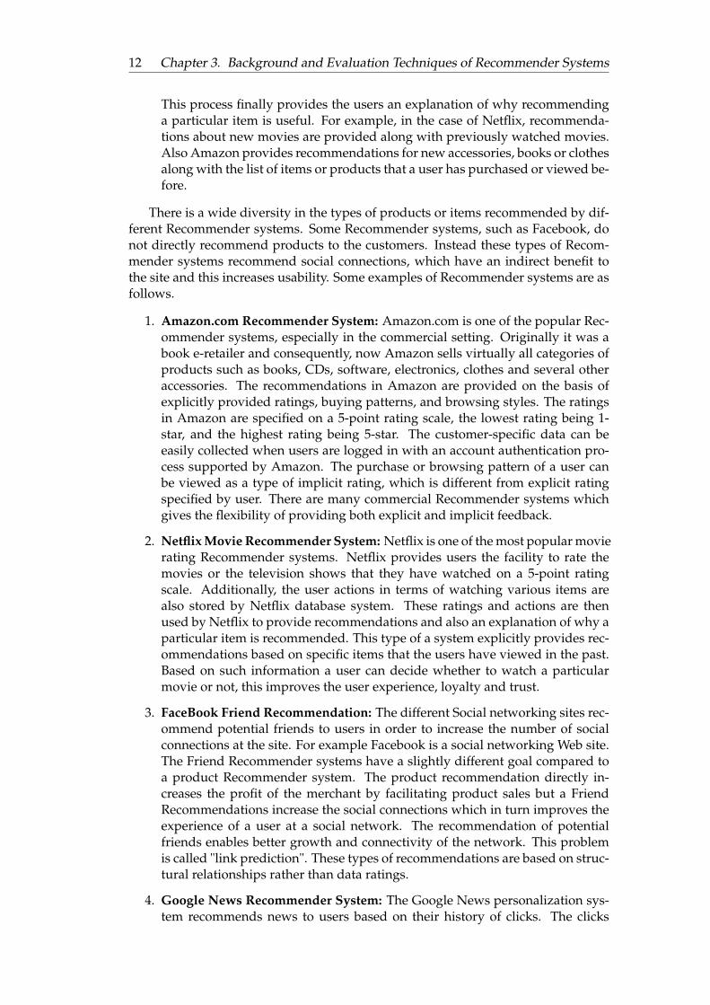
The recommendation algorithms are influenced by the systems used for tracking rat-ings. The ratings are often specified on a scale that indicates the specific level of likeor dislike of an item. It is possible for ratings to be continuous values, for examplethe Jester joke recommendation engine in which the ratings can take on any valuebetween -10 and 10. Usually, the ratings are interval-based, where a discrete set of or-dered numbers are used to quantify like or dislike. These types of ratings are calledinterval-based ratings. For example, a 5-point rating scale might be drawn from theset (1, 2, 3, 4, 5), in which 1 indicates strong dislike and 5 indicates strong affinitytowards an item. The number of possible ratings might vary with different systemswhich are used. The use of 5-point, 7-point, and 10-point ratings is particularly com-mon. The 5-star ratings system, is an example of interval based ratings. In 5 pointrating scale we interpret each rating as user’s level of interest . This interpretationmight vary across different websites. For example, Amazon uses a 5-star ratingssystem in which the 4-star point corresponds to “really liked it,” and the central 3-star point corresponds to “liked it.” Thus, in Amazon there are 3 favourable and 2non-favourable ratings. This is called Unbalanced Rating scale. In some cases, theremay be an even number of possible ratings, and the neutral rating might be missing.This approach is referred to as a forced choice rating system.
We can also use ordered categorical values such as (Strongly Disagree,Disagree,Neutral, Agree, Strongly Agree) in order to express our likes and dislikes. In general,such ratings are referred to as ordinal ratings. In binary ratings, the user may rep-resent his/her like or dislike for the item and nothing else. For example, the ratingsmay be 0, 1, or unspecified values. There is also concept of unary ratings, in whichthere is a way for a user to specify his liking for an item but no possibility to specifya dislike. These types of ratings are particularly used in the case of implicit feedbackdata sets. In these cases, customer preferences are derived from their actions and nottheir explicitly specified ratings. For example, the buying behavior of a customer canbe converted to unary ratings such as when a user buys an item, it can be viewed asa preference for the item. But at the same time the act of not buying an item does notindicate dislike towards an item. There are many social networks, such as Facebook,use “like” buttons, which provide the ability to express liking for an item but there isno mechanism to specify dislike for an item. We present a picture of 5 point Amazonrating system.
3.2.1 Explicit and Implicit Feedback
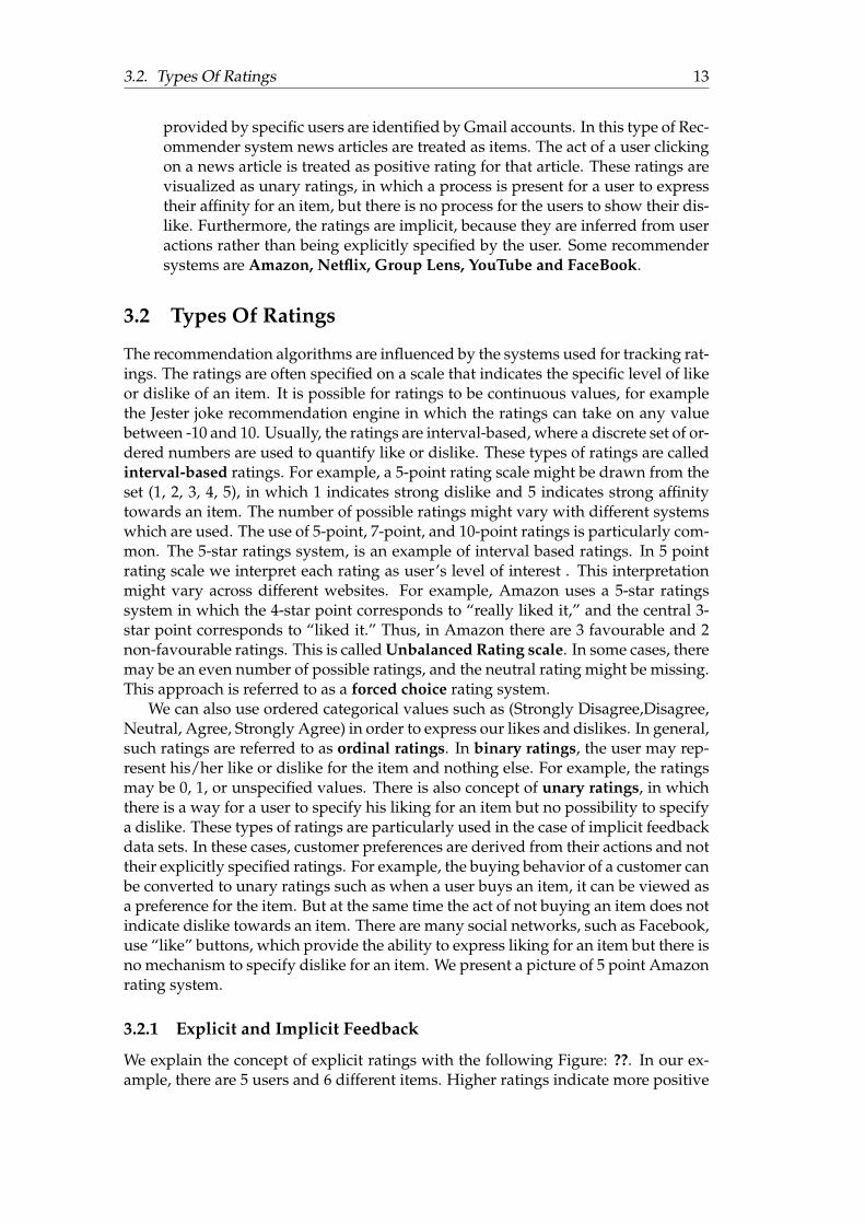
We explain the concept of explicit ratings with the following Figure: ??. In our ex-ample, there are 5 users and 6 different items. Higher ratings indicate more positive
14 Chapter 3. Background and Evaluation Techniques of Recommender Systems
FIGURE 3.1: Example of Amazon 5 point-interval ratings [7].
feedback . The missing entries correspond to unspecified preferences. We repre-sent the missing entries with "0". Here we present a small toy example. We haveconsidered the users and the items in form of a rating matrix. A ratings matrix issometimes referred to as a utility matrix. Although utility matrices are set to be thesame as the ratings matrices, it is possible for an application to explicitly transformthe ratings to utility values based on domain-specific criteria. Collaborative filteringapproach is then applied to the utility matrix rather than the ratings matrix. Actually,in practice, Collaborative filtering method work directly with the ratings matrix. Forcases in which the ratings are unary, the matrix is known as positive preference util-ity matrix since it allows only the specification of positive preferences. The matrixin Figure: ?? has different insights. In the matrix User2 and User5 are consideredsimilar users since they have both given same rating to the same product (Item1).Again, the same pair of users (User2 and User5) are different with respect to theproduct (Item4), since they have different ratings for that product. The User1, User2and User5 can be considered similar users since all of them have provided positivepreference for the same product (Item4).
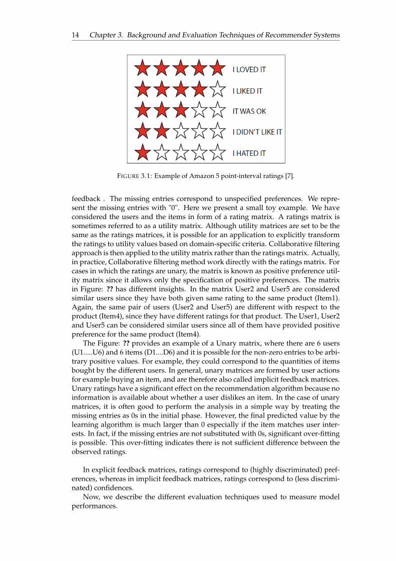
The Figure: ?? provides an example of a Unary matrix, where there are 6 users(U1.....U6) and 6 items (D1....D6) and it is possible for the non-zero entries to be arbi-trary positive values. For example, they could correspond to the quantities of itemsbought by the different users. In general, unary matrices are formed by user actionsfor example buying an item, and are therefore also called implicit feedback matrices.Unary ratings have a significant effect on the recommendation algorithm because noinformation is available about whether a user dislikes an item. In the case of unarymatrices, it is often good to perform the analysis in a simple way by treating themissing entries as 0s in the initial phase. However, the final predicted value by thelearning algorithm is much larger than 0 especially if the item matches user inter-ests. In fact, if the missing entries are not substituted with 0s, significant over-fittingis possible. This over-fitting indicates there is not sufficient difference between theobserved ratings.
In explicit feedback matrices, ratings correspond to (highly discriminated) pref-erences, whereas in implicit feedback matrices, ratings correspond to (less discrimi-nated) confidences.
Now, we describe the different evaluation techniques used to measure modelperformances.
3.3. Different Evaluation Techniques 15
FIGURE 3.2: Example of Utility Matrices.
FIGURE 3.3: Example of Unary Matrices.
3.3 Different Evaluation Techniques
The performance of a Recommender system can be measured by different evaluationtechniques. In this thesis we have used some evaluation techniques which are asfollows. In the context of our work we have tried to use simple formulas takingconcepts from reference documents.
1. The first evaluation technique that we have used is known as Area Under ROCCurve (AUC). This evaluation technique is used for recommending items. Forexample in case of user-item pair (u, i), the preference of a user u towards anitem i is considered as a function of time. Thus, the recommended item rankingfor user u is time dependent. So for a held-out triple (u, i, tui), our evaluationprocess consists of calculating how accurately a particular item denoted by iis ranked for specific user denoted by u at a particular time instance tui. Ourinput data set is split into training/validation/test sets by uniformly samplingfor each user u from user set an item i from item set(associated with a timestamp tui) to be used for validation (Vu) and another for testing (Tu). The rest
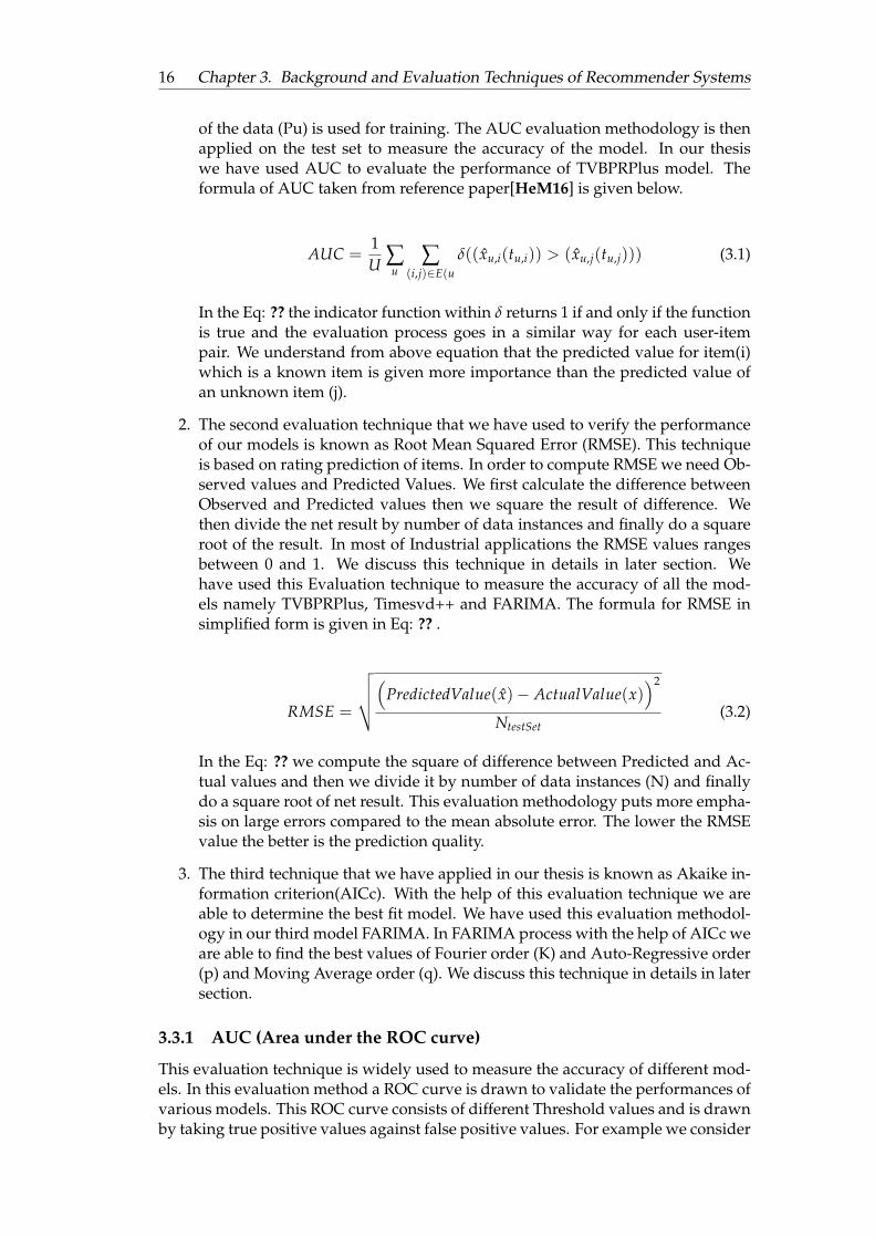
16 Chapter 3. Background and Evaluation Techniques of Recommender Systems
of the data (Pu) is used for training. The AUC evaluation methodology is thenapplied on the test set to measure the accuracy of the model. In our thesiswe have used AUC to evaluate the performance of TVBPRPlus model. Theformula of AUC taken from reference paper[HeM16] is given below.
AUC =1U ∑
u∑
(i,j)∈E(uδ((xu,i(tu,i)) > (xu,j(tu,j))) (3.1)
In the Eq: ?? the indicator function within δ returns 1 if and only if the functionis true and the evaluation process goes in a similar way for each user-itempair. We understand from above equation that the predicted value for item(i)which is a known item is given more importance than the predicted value ofan unknown item (j).
2. The second evaluation technique that we have used to verify the performanceof our models is known as Root Mean Squared Error (RMSE). This techniqueis based on rating prediction of items. In order to compute RMSE we need Ob-served values and Predicted Values. We first calculate the difference betweenObserved and Predicted values then we square the result of difference. Wethen divide the net result by number of data instances and finally do a squareroot of the result. In most of Industrial applications the RMSE values rangesbetween 0 and 1. We discuss this technique in details in later section. Wehave used this Evaluation technique to measure the accuracy of all the mod-els namely TVBPRPlus, Timesvd++ and FARIMA. The formula for RMSE insimplified form is given in Eq: ?? .
RMSE =
√√√√(PredictedValue(x)− ActualValue(x)
)2
NtestSet(3.2)
In the Eq: ?? we compute the square of difference between Predicted and Ac-tual values and then we divide it by number of data instances (N) and finallydo a square root of net result. This evaluation methodology puts more empha-sis on large errors compared to the mean absolute error. The lower the RMSEvalue the better is the prediction quality.
3. The third technique that we have applied in our thesis is known as Akaike in-formation criterion(AICc). With the help of this evaluation technique we areable to determine the best fit model. We have used this evaluation methodol-ogy in our third model FARIMA. In FARIMA process with the help of AICc weare able to find the best values of Fourier order (K) and Auto-Regressive order(p) and Moving Average order (q). We discuss this technique in details in latersection.
3.3.1 AUC (Area under the ROC curve)
This evaluation technique is widely used to measure the accuracy of different mod-els. In this evaluation method a ROC curve is drawn to validate the performances ofvarious models. This ROC curve consists of different Threshold values and is drawnby taking true positive values against false positive values. For example we consider
3.3. Different Evaluation Techniques 17
a positive class (P+) and a negative class (N-). Based on the position of the item in therespective classes there are different types of classification possible. If we consideran item to be a part of positive class then this type of classification is termed as truepositive. But in case if the item is not a member of the class then the classification istermed as false positive. Similarly, if the target item is a part of negative class thenthe classification is called true negative but if the item is not a member of the nega-tive class then it is termed as false negative. We have evaluated the performance ofTVBPRPlus using AUC technique. We provide an example of how AUC is appliedon TVBPRPlus below.
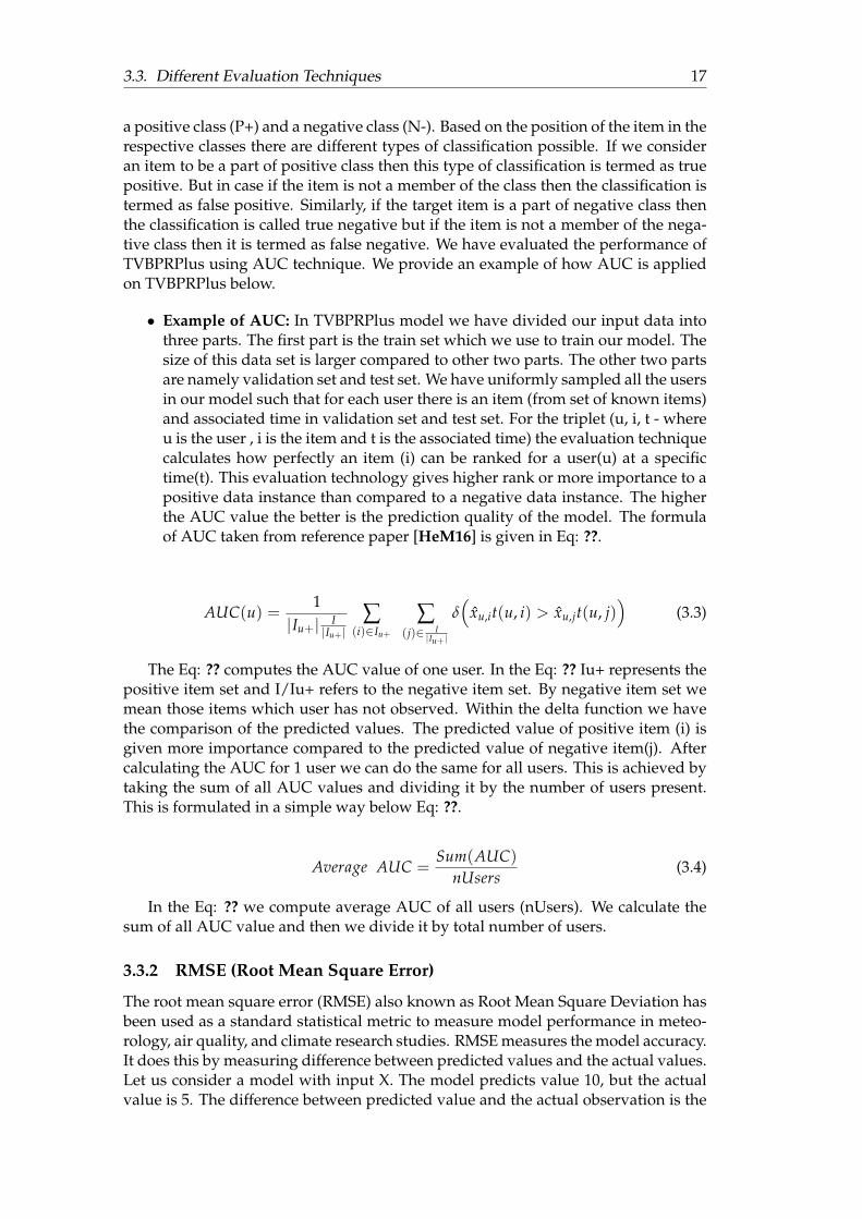
• Example of AUC: In TVBPRPlus model we have divided our input data intothree parts. The first part is the train set which we use to train our model. Thesize of this data set is larger compared to other two parts. The other two partsare namely validation set and test set. We have uniformly sampled all the usersin our model such that for each user there is an item (from set of known items)and associated time in validation set and test set. For the triplet (u, i, t - whereu is the user , i is the item and t is the associated time) the evaluation techniquecalculates how perfectly an item (i) can be ranked for a user(u) at a specifictime(t). This evaluation technology gives higher rank or more importance to apositive data instance than compared to a negative data instance. The higherthe AUC value the better is the prediction quality of the model. The formulaof AUC taken from reference paper [HeM16] is given in Eq: ??.
AUC(u) =1
|Iu+| I|Iu+|
∑(i)∈Iu+
∑(j)∈ I
|Iu+ |
δ(
xu,it(u, i) > xu,jt(u, j))
(3.3)
The Eq: ?? computes the AUC value of one user. In the Eq: ?? Iu+ represents thepositive item set and I/Iu+ refers to the negative item set. By negative item set wemean those items which user has not observed. Within the delta function we havethe comparison of the predicted values. The predicted value of positive item (i) isgiven more importance compared to the predicted value of negative item(j). Aftercalculating the AUC for 1 user we can do the same for all users. This is achieved bytaking the sum of all AUC values and dividing it by the number of users present.This is formulated in a simple way below Eq: ??.
Average AUC =Sum(AUC)
nUsers(3.4)
In the Eq: ?? we compute average AUC of all users (nUsers). We calculate thesum of all AUC value and then we divide it by total number of users.
3.3.2 RMSE (Root Mean Square Error)
The root mean square error (RMSE) also known as Root Mean Square Deviation hasbeen used as a standard statistical metric to measure model performance in meteo-rology, air quality, and climate research studies. RMSE measures the model accuracy.It does this by measuring difference between predicted values and the actual values.Let us consider a model with input X. The model predicts value 10, but the actualvalue is 5. The difference between predicted value and the actual observation is the
18 Chapter 3. Background and Evaluation Techniques of Recommender Systems
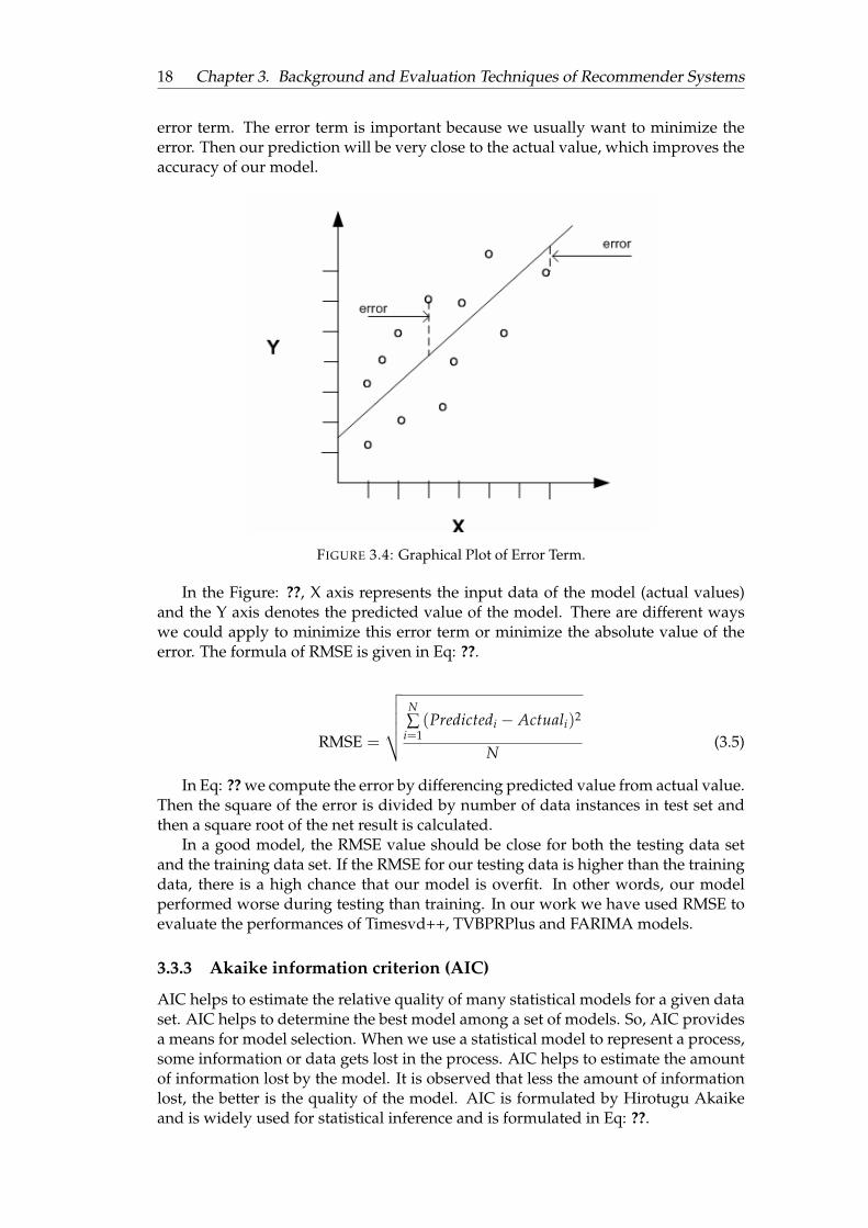
error term. The error term is important because we usually want to minimize theerror. Then our prediction will be very close to the actual value, which improves theaccuracy of our model.
FIGURE 3.4: Graphical Plot of Error Term.
In the Figure: ??, X axis represents the input data of the model (actual values)and the Y axis denotes the predicted value of the model. There are different wayswe could apply to minimize this error term or minimize the absolute value of theerror. The formula of RMSE is given in Eq: ??.
RMSE =
√√√√√ N∑
i=1(Predictedi − Actuali)2
N(3.5)
In Eq: ?? we compute the error by differencing predicted value from actual value.Then the square of the error is divided by number of data instances in test set andthen a square root of the net result is calculated.
In a good model, the RMSE value should be close for both the testing data setand the training data set. If the RMSE for our testing data is higher than the trainingdata, there is a high chance that our model is overfit. In other words, our modelperformed worse during testing than training. In our work we have used RMSE toevaluate the performances of Timesvd++, TVBPRPlus and FARIMA models.
3.3.3 Akaike information criterion (AIC)
AIC helps to estimate the relative quality of many statistical models for a given dataset. AIC helps to determine the best model among a set of models. So, AIC providesa means for model selection. When we use a statistical model to represent a process,some information or data gets lost in the process. AIC helps to estimate the amountof information lost by the model. It is observed that less the amount of informationlost, the better is the quality of the model. AIC is formulated by Hirotugu Akaikeand is widely used for statistical inference and is formulated in Eq: ??.
3.3. Different Evaluation Techniques 19
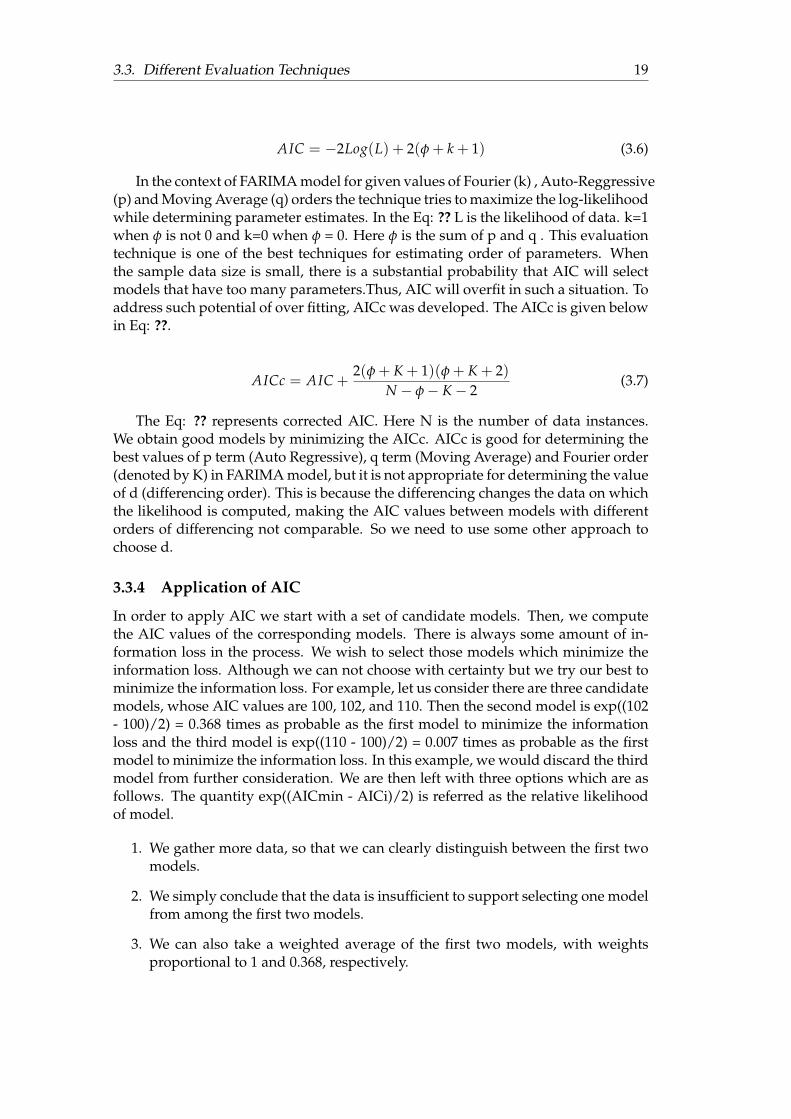
AIC = −2Log(L) + 2(φ + k + 1) (3.6)
In the context of FARIMA model for given values of Fourier (k) , Auto-Reggressive(p) and Moving Average (q) orders the technique tries to maximize the log-likelihoodwhile determining parameter estimates. In the Eq: ?? L is the likelihood of data. k=1when φ is not 0 and k=0 when φ = 0. Here φ is the sum of p and q . This evaluationtechnique is one of the best techniques for estimating order of parameters. Whenthe sample data size is small, there is a substantial probability that AIC will selectmodels that have too many parameters.Thus, AIC will overfit in such a situation. Toaddress such potential of over fitting, AICc was developed. The AICc is given belowin Eq: ??.
AICc = AIC +2(φ + K + 1)(φ + K + 2)
N − φ− K− 2(3.7)
The Eq: ?? represents corrected AIC. Here N is the number of data instances.We obtain good models by minimizing the AICc. AICc is good for determining thebest values of p term (Auto Regressive), q term (Moving Average) and Fourier order(denoted by K) in FARIMA model, but it is not appropriate for determining the valueof d (differencing order). This is because the differencing changes the data on whichthe likelihood is computed, making the AIC values between models with differentorders of differencing not comparable. So we need to use some other approach tochoose d.
3.3.4 Application of AIC
In order to apply AIC we start with a set of candidate models. Then, we computethe AIC values of the corresponding models. There is always some amount of in-formation loss in the process. We wish to select those models which minimize theinformation loss. Although we can not choose with certainty but we try our best tominimize the information loss. For example, let us consider there are three candidatemodels, whose AIC values are 100, 102, and 110. Then the second model is exp((102- 100)/2) = 0.368 times as probable as the first model to minimize the informationloss and the third model is exp((110 - 100)/2) = 0.007 times as probable as the firstmodel to minimize the information loss. In this example, we would discard the thirdmodel from further consideration. We are then left with three options which are asfollows. The quantity exp((AICmin - AICi)/2) is referred as the relative likelihoodof model.
1. We gather more data, so that we can clearly distinguish between the first twomodels.
2. We simply conclude that the data is insufficient to support selecting one modelfrom among the first two models.
3. We can also take a weighted average of the first two models, with weightsproportional to 1 and 0.368, respectively.
20
Chapter 4
Prediction Models
In our thesis we have worked with three different prediction models which areTVBPRPlus, Timesvd++ and FARIMA. We have applied these models to predict thefuture trend of a specific product based on Amazon fashion dataset. The efficiencyand accuracy of these models are evaluated using different evaluation methods suchas RMSE, AUC and AICc. In this chapter we discuss the implemented models in de-tails.
4.1 TVBPRPlus model
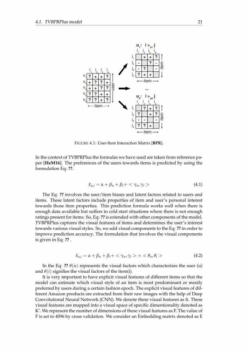
TVBPRPlus model is based on Collaborative Filtering. The model determines theusers fashion aware personalized ranking based on the past feedback (user reviews)of users. The model is capable of capturing both the temporal and visual dynamicsof data. The users are highly influenced by the visual styles of different items. Thesevisual styles or features of various product vary over different fashion epochs. Thismodel is able to uncover these visual features which has a direct impact on userschoices. TVBPRPlus is visually aware, temporally evolving, interoperable, scalableand personalized. The model aims at accurately recommending an item (i) for a user(u) at time period (t) which will fit his purpose of need. For example if a user haspurchased fashion products such as sunglasses and perfumes then the model willrecommend the same user similar category of items such as a hat or a watch etcwhich will serve the needs of the user. TVBPRPlus model follows the basic formu-lation of matrix factorization, where the users and the items are presented in formof a matrix. A mapping is performed between the users and the items by observingthe values in the matrix. This type of a matrix is known as User-Item Interactionmatrix. For example if a cell corresponding to a user and an item contains 1 valueor + sign (positive sign), then it is considered that the user has shown interest in thecorresponding item. Such an item is called a positive item and if the value in a cellof the matrix is -1 or - sign (negative sign), then it is understood that the user hasnot preferred that particular item. Such an item is referred as negative item. Theuser-item matrix is divided into two sub matrixes. The values used in the matrix areassumed to be ratings given by users to the items. We present a picture of a user-item matrix from reference paper [BPR] in Figure: ??. In this figure user specificpairwise preferences between a pair of items is created. The + sign indicates thatthe user prefers item i over item j and – sign indicates that user prefers j item overi. The question mark sign signifies that the user has not visited those items. Thus,the user-item interaction matrix helps to determine the user’s preference towardsdifferent items.
We have used Latent Factor Model or matrix factorization to implement TVBPRPlus.According to the Latent Factor model the users and items are mapped to latent space.
4.1. TVBPRPlus model 21
FIGURE 4.1: User-Item Interaction Matrix [BPR].
In the context of TVBPRPlus the formulas we have used are taken from reference pa-per [HeM16]. The preferences of the users towards items is predicted by using theformulation Eq: ??.
xu,i = α + βu + βi+ < γu, γi > (4.1)
The Eq: ?? involves the user/item biases and latent factors related to users anditems. These latent factors include properties of item and user’s personal interesttowards those item properties. This prediction formula works well when there isenough data available but suffers in cold start situations where there is not enoughratings present for items. So, Eq: ?? is extended with other components of the model.TVBPRPlus captures the visual features of items and determines the user’s interesttowards various visual styles. So, we add visual components to the Eq: ?? in order toimprove prediction accuracy. The formulation that involves the visual componentsis given in Eq: ?? .
xu,i = α + βu + βi+ < γu, γi > + < θu, θi > (4.2)
In the Eq: ?? θ(u) represents the visual factors which characterizes the user (u)and θ(i) signifies the visual factors of the item(i).
It is very important to have explicit visual features of different items so that themodel can estimate which visual style of an item is most predominant or mostlypreferred by users during a certain fashion epoch. The explicit visual features of dif-ferent Amazon products are extracted from their raw images with the help of DeepConvolutional Neural Network (CNN). We denote these visual features as fi. Thesevisual features are mapped into a visual space of specific dimentionality denoted asK’. We represent the number of dimensions of these visual features as F. The value ofF is set to 4096 by cross validation. We consider an Embedding matrix denoted as E
22 Chapter 4. Prediction Models
(K’ * F) which linearly embeds the high dimensional features extracted from productimages into a lower dimensional visual style space (K’). The visual features of itemsare formulated in Eq: ?? . It is denoted as θi.
θi = E ∗ fi (4.3)
In the Eq: ?? E (k‘ * F) represents the embedding matrix and fi denotes the ex-plicit visual features extracted from the images of items using CNN. The embeddingmatrix E is able to uncover the visual factors of items and these visual factors highlyinfluence user preferences.
The visual and as well as the Non-visual components of the model varies overtime. The temporal dynamics related to visual and Non-visual factors are as follows.
1. Time Dependent visual factors.
2. Temporally Changing visual bias.
3. Time Dependent Non- visual Factors.
4.1.1 Time Dependent visual factors
In the fashion world new items with different visual styles always emerge in differ-ent fashion epochs. For example we consider the shoes of "Puma". This shoe has aparticular visual style but this visual may lose its significance when a new version of"Puma" shoes with new visual features evolves in market. So, we need to design theEmbedding matrix (E) to be time dependent. The Embedding Matrix should be ableto capture different types of fashion dynamics over time. This is called TemporalAttractiveness Drift.
• Temporal Attractiveness Drift: The visual features of different products gainor lose their importance in various time zones. Thus, the attractiveness of itemschange over time. In order to determine which visual feature is most attractiveduring a time period, it is necessary to capture this temporal drift in visualstyles. So, the Embedding matrix is extended with temporal components. Thistime sensitive Embedding matrix is given in Eq: ??.
E(t) = E + ∆E(t) (4.4)
In the Eq: ?? the stationary component of the model is captured by E and the timedependent part is handled by delta E. This Embedding matrix is capable of capturingdifferent visual styles of items over several epochs.So, now the visual factors of itemsare extended with time dependent Embedding matrix. This is formulated in Eq: ??
θi(t) = E(t) ∗ fi (4.5)
In the Eq: ?? the E(t) denotes time dependent embedding matrix and fi are thevisual features extracted from images of items using CNN.
4.1. TVBPRPlus model 23
As new fashionable items or products evolve with time, the different visual di-mensions are weighted differently by different users. For example users may payless attention to a dimension describing bright colour if they are already tolerant tobright colours. So, a temporal weighing vector is considered to capture the usersevolving emphasis on different visual dimensions. The formulation of θ(i) is ex-tended with the weighing vector.
θi(t) = E ∗ fi �ω(t) (4.6)
In the Eq: ?? � refers to Hadamard product. So, now the visual factors related toitems can be formulated in Eq: ??.
θi(t) = E ∗ fi �ω(t)︸ ︷︷ ︸Base
+∆E(t) fi︸ ︷︷ ︸Deviation
(4.7)
The Eq: ?? is valid for global structures but to model or capture the personalinterest of each user over time we introduce the concept of Temporal Personal Drift.
• Temporal Personal Drift: The personal interests of users vary over time. Theinterests of users are influenced by both outside evolving fashion trends andhis/her personal taste. In this case we consider certain concepts of Timesvd++model (discussed in details later). The time sensitive visual factors of users isformulated based on Timesvd++ model.
θu(t) = θu + sign(t− tu) · |t− tu|kηu (4.8)
The Eq:?? explains the deviation of user u at time t from his or her mean feedbackdate tu.
4.1.2 Temporally evolving visual bias
In addition to the temporal visual factors we also use a time dependent visual bias.The visual bias helps to capture the changes in item appearance using low rankstructures. So, we can use high rank structures to capture other variation for exampleper-user dynamics and per-dimension dynamics. This is computed as a product of<ß(t),fi>, ß(t) is a time dependent F dimensional vector. Visual Bias helps to improvethe performance of the model and is also good for visualization. The formulationfor the visual bias is given in Eq: ??.
β(t) = β� b(t) + ∆β(t) (4.9)
4.1.3 Time Dependent Non- visual Factors
The Non-visual components also play a vital role in the prediction process of themodel. In our context the Non-visual components are related to item profiles suchas category of an item. There are two approaches to handle Non-visual factors. Theyare as follows.
24 Chapter 4. Prediction Models
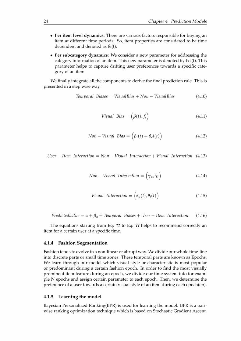
• Per item level dynamics: There are various factors responsible for buying anitem at different time periods. So, item properties are considered to be timedependent and denoted as ßi(t).
• Per subcategory dynamics: We consider a new parameter for addressing thecategory information of an item. This new parameter is denoted by ßci(t). Thisparameter helps to capture drifting user preferences towards a specific cate-gory of an item.
We finally integrate all the components to derive the final prediction rule. This ispresented in a step wise way.
Temporal Biases = VisualBias + Non−VisualBias (4.10)
Visual Bias =(
β(t), fi
)(4.11)
Non−Visual Bias =(
βi(t) + βci(t))
(4.12)
User− Item Interaction = Non−Visual Interaction + Visual Interaction (4.13)
Non−Visual Interaction =(
γu, γi
)(4.14)
Visual Interaction =(
θu(t), θi(t))
(4.15)
Predictedvalue = α + βu + Temporal Biases + User− Item Interaction (4.16)
The equations starting from Eq: ?? to Eq: ?? helps to recommend correctly anitem for a certain user at a specific time.
4.1.4 Fashion Segmentation
Fashion tends to evolve in a non-linear or abrupt way. We divide our whole time-lineinto discrete parts or small time zones. These temporal parts are known as Epochs.We learn through our model which visual style or characteristic is most popularor predominant during a certain fashion epoch. In order to find the most visuallyprominent item feature during an epoch, we divide our time system into for exam-ple N epochs and assign certain parameter to each epoch. Then, we determine thepreference of a user towards a certain visual style of an item during each epoch(ep).
4.1.5 Learning the model
Bayesian Personalized Ranking(BPR) is used for learning the model. BPR is a pair-wise ranking optimization technique which is based on Stochastic Gradient Ascent.
4.2. Timesvd++ 25
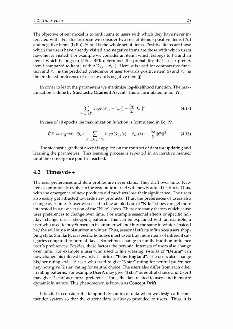
The objective of our model is to rank items to users with which they have never in-teracted with. For this purpose we consider two sets of items - positive items (Pu)and negative items (I/Pu). Here I is the whole set of items. Positive items are thosewhich the users have already visited and negative items are those with which usershave never visited. For example we consider an item i which belongs to Pu and anitem j which belongs to I/Pu. BPR determines the probability that a user prefersitem i compared to item j with σ(xu,i − xu,i). Here, σ is used for comparative func-tion and xu,i is the predicted preference of user towards positive item (i) and xu,j isthe predicted preference of user towards negative item (j).
In order to learn the parameters we maximize log-likelihood function. The max-imization is done by Stochastic Gradient Ascent. This is formulated in Eq: ??.
∑(u,i,j)∈Ds
logσ(xu,i − xu,j)−λθ
2||Θ||2 (4.17)
In case of 10 epochs the maximization function is formulated in Eq: ??.
Θ∧ = argmax Θ,∧ ∑(u,i,j,tu,i)∈Ds
logσ(xu,i(t)− xu,j(t))−λθ
2||Θ||2 (4.18)
The stochastic gradient ascent is applied on the train set of data for updating andlearning the parameters. This learning process is repeated in an iterative manneruntil the convergence point is reached.
4.2 Timesvd++
The user preferences and item profiles are never static. They drift over time. Newitems continuously evolve in the economic market with newly added features. Thus,with the emergence of new products old products lose their significance. The usersalso easily get attracted towards new products. Thus, the preferences of users alsochange over time. A user who used to like an old type of "Nike" shoes can get moreinterested in a new version of the "Nike" shoes. There are many factors which causeuser preferences to change over time. For example seasonal effects or specific hol-idays change user’s shopping pattern. This can be explained with an example, auser who used to buy Sunscreen in summer will not buy the same in winter. Insteadhe/she will buy a moisturizer in winter. Thus, seasonal effects influences users shop-ping style. Similarly, on specific holidays most users buy more items of different cat-egories compared to normal days. Sometimes change in family tradition influenceuser’s preferences. Besides, these factors the personal interests of users also changeover time. For example a user who used to like wearing T-shirts of "Denim" cannow change his interest towards T-shirts of "Peter England". The users also changehis/her rating style. A user who used to give "3 star" rating for neutral preferencemay now give "2 star" rating for neutral choice. The users also differ from each otherin rating patterns. For example UserA may give "3 star" as neutral choice and UserBmay give "2 star" as neutral preference. Thus, the data related to users and items aredynamic in nature. This phenomenon is known as Concept Drift.
It is vital to consider the temporal dynamics of data when we design a Recom-mender system so that the current data is always provided to users. Thus, it is
26 Chapter 4. Prediction Models
necessary for us to build models which are temporal aware. One of such modelsis Timesvd++ which captures the drifting user interests and item properties. Themodel comprises of main two components namely, time dependent Baseline predic-tors which captures much of temporal dynamics in data and Use-Item interactionfactors which are responsible for capturing the dynamic user behaviour and chang-ing item profiles.
Timesvd++ is based on Collaborative Filtering (CF) which relies on past user be-haviour such as past user transactions or user preferences. CF does not require do-main knowledge and there is no need to explicitly create user/item profiles. Whenenough data is collected CF method is most preferred. In CF based technique werely on past user purchase histories or preferences which helps us to uncover com-plex patterns which would otherwise be difficult to explore with only data attributes.This methodology is used by many popular commercial Recommender systems suchas Amazon, Netflix. In order to give recommendations CF technique needs to com-pare different things such as items against users. CF supports two main approacheswhich are as follows.
1. Neighbourhood approach.
2. latent factor model.
We briefly discuss the different approaches of Collaborative Filtering.
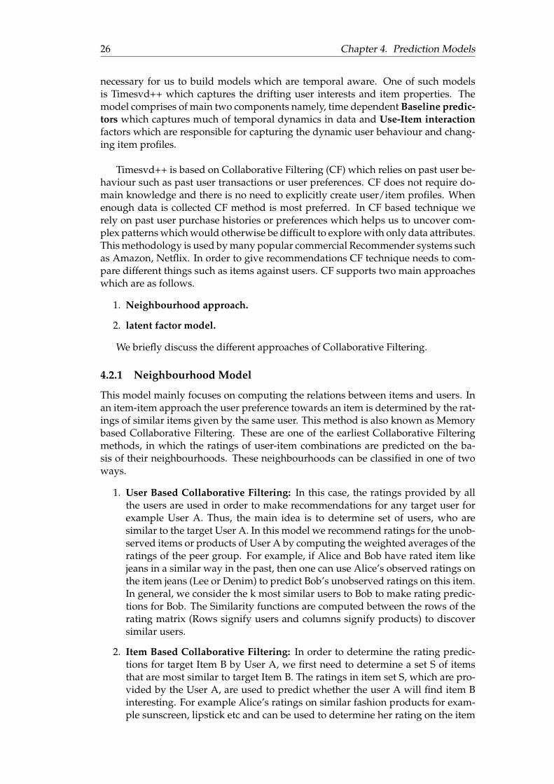
4.2.1 Neighbourhood Model
This model mainly focuses on computing the relations between items and users. Inan item-item approach the user preference towards an item is determined by the rat-ings of similar items given by the same user. This method is also known as Memorybased Collaborative Filtering. These are one of the earliest Collaborative Filteringmethods, in which the ratings of user-item combinations are predicted on the ba-sis of their neighbourhoods. These neighbourhoods can be classified in one of twoways.
1. User Based Collaborative Filtering: In this case, the ratings provided by allthe users are used in order to make recommendations for any target user forexample User A. Thus, the main idea is to determine set of users, who aresimilar to the target User A. In this model we recommend ratings for the unob-served items or products of User A by computing the weighted averages of theratings of the peer group. For example, if Alice and Bob have rated item likejeans in a similar way in the past, then one can use Alice’s observed ratings onthe item jeans (Lee or Denim) to predict Bob’s unobserved ratings on this item.In general, we consider the k most similar users to Bob to make rating predic-tions for Bob. The Similarity functions are computed between the rows of therating matrix (Rows signify users and columns signify products) to discoversimilar users.
2. Item Based Collaborative Filtering: In order to determine the rating predic-tions for target Item B by User A, we first need to determine a set S of itemsthat are most similar to target Item B. The ratings in item set S, which are pro-vided by the User A, are used to predict whether the user A will find item Binteresting. For example Alice’s ratings on similar fashion products for exam-ple sunscreen, lipstick etc and can be used to determine her rating on the item
4.2. Timesvd++ 27
eyeliner. Similarity functions are computed between the columns of the rat-ings matrix to discover similar items. The columns of the rating matrix signifythe items.
The advantages of memory-based techniques or neighbourhood model are asfollows.
1. These models are simple to implement.
2. The resulting recommendations achieved from these models are often easy toexplain and understand.
But at the same time these models also suffer from some limitations such as.
1. The memory-based algorithms do not work very well with sparse rating ma-trices. For example, it might be difficult to identify enough number of similarusers to Bob. In such cases, it is difficult to predict Bob’s rating. Thus, thesemethods do not have full coverage of rating predictions. But the lack of cover-age is not a big problem when we only consider the top K items.
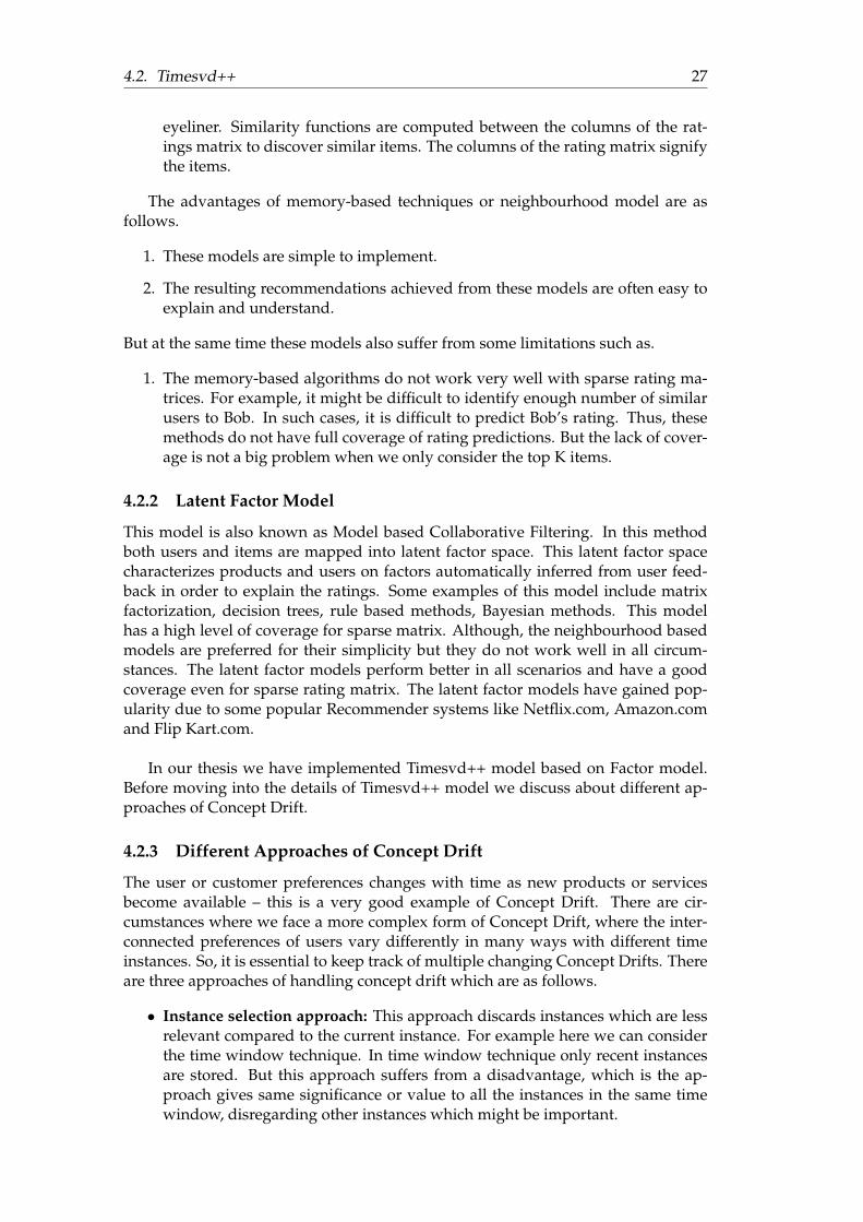
4.2.2 Latent Factor Model
This model is also known as Model based Collaborative Filtering. In this methodboth users and items are mapped into latent factor space. This latent factor spacecharacterizes products and users on factors automatically inferred from user feed-back in order to explain the ratings. Some examples of this model include matrixfactorization, decision trees, rule based methods, Bayesian methods. This modelhas a high level of coverage for sparse matrix. Although, the neighbourhood basedmodels are preferred for their simplicity but they do not work well in all circum-stances. The latent factor models perform better in all scenarios and have a goodcoverage even for sparse rating matrix. The latent factor models have gained pop-ularity due to some popular Recommender systems like Netflix.com, Amazon.comand Flip Kart.com.
In our thesis we have implemented Timesvd++ model based on Factor model.Before moving into the details of Timesvd++ model we discuss about different ap-proaches of Concept Drift.
4.2.3 Different Approaches of Concept Drift
The user or customer preferences changes with time as new products or servicesbecome available – this is a very good example of Concept Drift. There are cir-cumstances where we face a more complex form of Concept Drift, where the inter-connected preferences of users vary differently in many ways with different timeinstances. So, it is essential to keep track of multiple changing Concept Drifts. Thereare three approaches of handling concept drift which are as follows.
• Instance selection approach: This approach discards instances which are lessrelevant compared to the current instance. For example here we can considerthe time window technique. In time window technique only recent instancesare stored. But this approach suffers from a disadvantage, which is the ap-proach gives same significance or value to all the instances in the same timewindow, disregarding other instances which might be important.
28 Chapter 4. Prediction Models
• Instance weighting approach: In this approach the instances are weightedbased on the estimated relevance. Also in this approach a time decay functionis used for under weighted instances which decay with time.
• Ensemble Learning: In this approach a group of predictors produce the finalresult. These predictors are weighted by their perceived relevance. For exam-ple the predictors which are more popular in the recent time span have highervalues.
We follow some general rules or guidelines for capturing the drifting user pref-erences. Some of these rules are as follows.
• We must consider models which capture user behaviour or buying patternsthroughout the time span not only the present user pattern. In this way we areable to extract data or information at each time point in the time line.
• We must adopt models which capture multiple changing Concept Drifts, sincesome drifts are user dependent and some are item dependent.
• The Concept Drifts which we collect for individual users and items must becombined in a single frame, so that there are interactions among all users anditems to get a high level pattern.
4.2.4 Timesvd++ Implementation Based on Matrix Factorization
Matrix factorization method maps both users and items into a joint latent factorspace of certain dimensionality which we denote by f. The user-item interactions aremodeled as inner product in that space. The latent space tries to explain user ratingsby characterizing users and items with factors relevant to the application domain(For example casual dress vs party dress for clothes). Each user is associated witha vector and each item is associated with another vector. The item vector measuresthe extent to which item i possesses these factors while the user vector measures theextent of interest of a user in these factors. Even in cases where independent im-plicit feedback is absent, one can capture the rating by accounting for which itemsusers rate, regardless of their rating value. To this end, a second set of item factorsis added, relating each item i to a factor vector denoted by Yi. The formulas that wehave used in the context of Timesvd++ are taken from reference paper [Koren10].The rating is predicted as an inner product of user and item factors.
ru,i = qTi pu (4.19)
In the Eq: ?? pu denotes the set of users (can also be considered as vector) andqi (can also be considered as vector) signifies the set of items. In order to learn thevectors pu and qi, we minimize the regularized squared error.
min q∗, p∗ ∑(u,i,t)∈K
(ru,i − qTi pu)
2 + λ(||qi||2 + ||pu||2) (4.20)
In the Eq: ??, λ controls the extent of regularization. The minimization is per-formed by Stochastic Gradient Descent. Thus, the factor model captures the inter-action between users and items in a well manner. The different parameters of themodel are discussed below.
4.2. Timesvd++ 29
• Baseline Predictors: In Factor model most of the observed rating values iseither due to users or items independently of their interaction. For exampleit is the nature of some users to give higher ratings to items and some itemseventually receive higher ratings compared to other items. As described in thepaper [Koren10] we use baseline predictors to capture those effects which donot involve user-item interaction. The baseline predictors capture the temporaldynamics in data, so it must be modelled accurately. The baseline predictorsfor an unknown rating are given in Eq: ??.
bu,i = µ + bu + bi (4.21)
In the Eq: ??, µ denotes the average rating. The bu and bi denotes the user anditem biases respectively. The baseline predictors must be integrated into thefactor model, so we extend the Eq:?? and the new Eq: ?? is formulated.
AUC =1U ∑
u∑
(i,j)∈E(uδ((xu,i(tu,i)) > (xu,j(tu,j))) (4.22)
In order to achieve better accuracy we consider the implicit information aboutthe items which are rated, regardless of their rating value. We consider a sec-ond set of item vector denoted by Yi. These new set of items helps to determinethe user characteristics based on the items that they have rated. After incorpo-rating this new set of items the formulation Eq: ?? looks as follows.
ru,i = µ + bu + bi + qTi
(pu + |R(u)|−
12 ∑
(j)∈R(u)
)(4.23)
In the Eq: ?? R(u) denotes the set of items rated by user. The bu and bi arethe user and item biases. The user preferences are denoted by vector pu.TheBaseline predictors are not fixed they vary over time. So we have added thetemporal component to the Baseline Predictors.
• Time changing Baseline Predictors: Regarding baseline predictors there aretwo major temporal effects. The first one is related to items and the secondone is related to users. The popularity of items drift with time. For examplea particular type of women jacket is popular in winter season but it may loseits popularity in the summer season, a particular type of men shoes mightbecome popular during some period of time but later it may lose its popularity.The users also change their ratings or preferences over time. For example auser who used to rate average items by 4 star rating, later changes his/herrating pattern by giving average rating as 3 star due to several reasons. So, theBaseline predictors are time dependent. The time sensitive equation of baselinepredictors is formulated in Eq: ??.
bu,i(t) = µ + bu(t) + bi(t) (4.24)
30 Chapter 4. Prediction Models
In the Eq: ?? the user and item biases vary over time.The user effects changeon daily basis. So, there are inconsistencies in user behaviour. Therefore, weneed finer resolution to capture user biases. The item biases do not change ona daily basis. So, the item biases are easier to capture as they do not need fineresolution. To deal with item biases we consider splitting the item biases intotime based bins. The choice of how to split the item biases into time based binsdepends on the application. If we need enough rating per bin then larger binsare required and if we require finer resolution then smaller bins are needed.In our work we have used 30 bins spanning all days in the dataset. The itembias is split into stationary part and a time dependent part. The formulationfor item bias is given in Eq: ??
bi(t) = bi + bi,Bin(t) (4.25)
In the Eq: ?? a day t is associated with an integer Bin(t), where t can be anynumber from 1 to 30. The user biases are difficult to capture since they haveshort lived temporal effects. We use a liner function to capture the gradualdrift in user behaviour. This is given by the following formulation in Eq: ??.
devu(t) = sign(t− tu) · |t− tu|β (4.26)
In the Eq: ?? the mean date of rating is denoted by tu for a user u and theuser gives his/her rating on a particular day t. We express the time distanceor difference of number of days between t and tu by | t - tu|. We consider thevalue of ß to be 0.4 by cross validation [Koren10]. Thus, the final equation fortime changing user bias is given in the Eq: ??.
b(1)u (t) = bu + αu · devu(t) (4.27)
Apart from the gradual concept drift there are sudden drifts emerging as spikesfrom many applications. For example in any application we often find a partic-ular user giving multiple ratings in a single day. This may be due to the moodof the user on that day. These effects are short lived and generally do not spanmore than a single day. In order to address such short lived effects we use anew parameter denoted by bu,t. This newly introduced parameter capturesday specific variability. This parameter alone is not appropriate for capturingthe user bias since it misses all the necessary data that span more than a singleday. Thus, it serves as an additive component to the previously described userbias. This is formulated in Eq: ??.
b(3)u (t) = bu + αu · devu(t) + bu,t (4.28)
Next, we combine the user and item biases which vary over time to derive thefinal equation for temporally varying baseline predictors. This is given in Eq.??.
4.2. Timesvd++ 31
bu,i(t) = µ + bu + αu · devu(t) + bu,t + bi + bi,Bin(t) (4.29)
Besides, temporal effects we can use the same methodology to capture peri-odic effects. For example some items are more popular in certain seasons suchas the jackets and winter shoes are more popular in winter season and sun-glasses and T-shirts are more popular in summer season. In order to capturethese periodic effects we introduce a new parameter. This newly introducedparameter is modelled with item bias. This is presented in the Eq: ??.
bi(t) = bi + bi,Bin(t) + bi,period(t) (4.30)
In the Eq: ?? the periodic effects regarding the items is captured by the param-eter bi,period(t).
The periodic effects are also observed in case of users. For example some usershave different shopping patterns in the weekends or on specific holidays. Thisperiodic effect is captured by using a new parameter in a similar way like incase of items. This is given by the following Eq: ??.
bu(t) = bu + αu · devu(t) + bu,t + bu,period(t) (4.31)
In the Eq: ?? periodic effect regarding users is captured by the parameterbu,period(t).
There is another temporal effect which is related to baseline predictors, it isthe changing scale of user ratings. For example different users have differentrating scale and even a single user can also change his/her rating style. Inorder to address this type of a temporal effect we add a time dependent scalingfeature to the baseline predictors denoted by cu(t). This is given by the Eq. ?? .
bu,i(t) = µ + bu + αu · devu(t) + bu,t +(
bi + bi,Bin(t))· cu(t) (4.32)
In the Eq. ?? cu(t) represents the day specific variability. This multiplicativefactor helps to reduce the RMSE value, which further improves the accuracyof the model. The temporal dynamics also affect the user preferences or inother words they affect the interaction between users and items. The prefer-ences of users vary with time. For example a user who used to like wearingsunglasses of "RayBan" can now change his/her preference and switch to sun-glasses of "RainBow" brand. In order to model user preferences we use a vectorrepresented by p(u) and it is taken as function of time. This is given in Eq: ??.
pu,k(t) = pu,k + αu,k · devu(t) + pu,k,t (4.33)
32 Chapter 4. Prediction Models
In the Eq: ??, puk captures the stationary portion of this factor and puk,t cap-tures the day specific variability and k= 1....f. Finally, we incorporate all themodel parameters and deduce the final equation of Timesvd++. This is givenin Eq: ??.
ru,i = µ + bu(t) + bi(t) + qTi
(pu(t) + |R(u)|−
12 ∑
(j)∈R(u)yj
)(4.34)
In the Eq: ?? all the model parameters drifts over time. We divide our inputdata set into train set and test set. We use the train set to train and learn the model.The learning is done by stochastic gradient descent and then we validate the modelusing the test set. We compute RMSE on the test set to measure the accuracy of themodel. We validate the performance of our model using different experiments, forexample we vary the dimensionality (f) of latent space. We take different f values like10, 20, 50, 100 and 200. We observe that the RMSE value decreases with increasingdimensionality. The lower the RMSE the better is the model accuracy. There areother experiments performed on the model to test its efficiency and accuracy. Wediscuss these experiments in details in later section.
4.3 Fourier Assisted ARIMA or FARIMA
In the economic market the user preferences and item profiles change frequentlywith the emergence of new products in the market, this leads to dynamic modellingof users and items in the personalized Recommender systems. In the previous meth-ods we focused on product level modelling, where user preferences are modelledbased on their purchase histories (Collaborative Filtering). But it is observed thatproduct level modelling suffers from lack of data since some users may rate fewitems compared to the huge set of items in the whole system. So, now we movefrom product level modelling to feature level modelling, where we extract the do-main knowledge or explicit features in a specific product domain. The feature levelmodelling grants the ability to predict the user preferences through time series anal-ysis. The expanded feature space of this methodology helps to make cold start rec-ommendations for users with few purchasing records. The product level modellingapproach discards the cold start users for example users with less than 20 reviews.But in real world applications this is not feasible since these cold start users consti-tute a major part of the system.
Our Recommender systems must be designed in such a way so that it behavesintelligently to recommend items or products that fit the current user needs. Forexample in summer users normally use sunscreens to protect their skin from strongUV radiation of the sun but in winter users buy moisturizing cream due to cold anddry weather. If the Recommender system always considers the purchasing historiesfor recommending products to users instead of dynamic modelling of user prefer-ences then the system will recommend products like sunscreen in winter. An itemalso receives new reviews from users which make it profile drift dynamically overtime. Thus, we must build our Recommender systems such that it will recommenditems which fit the purpose of users.
4.3. Fourier Assisted ARIMA or FARIMA 33
In order to track new fashionable items and provide recommendations timely weanalyze the time series on daily basis. In this context, we use the Auto-RegressiveIntegrated Moving Average (ARIMA) model. The ARIMA model is widely usedfor monthly, yearly, quarterly time series analysis, however, the year-long period(around m = 365) of daily time series makes the ARIMA models in-feasible in prac-tice due to the huge computational cost. In order to address this problem we developFourier-assisted Auto-Regressive Integrated Moving Average (FARIMA) to capturethe seasonal component of the time series and use ARIMA to handle the residuals.
We first provide a brief description of time series decomposition analysis andthen gradually move to the working of FARIMA model.
4.3.1 Time Series Decomposition
Time series analysis and modelling have many business and social applications. It isextensively used to forecast company sales, product demand, stock market trends,agricultural production etc. A time series is a sequential set of data points which ismeasured typically over successive times. It is mathematically defined as a set ofvectors x(t),t = 0,1,2,... where t represents the time elapsed. We consider the vari-able x(t) as a random variable. The measurements in a time series are always in aproper chronological order. The time series containing records of a single variable istermed as uni-variate. But if records of more than one variable are considered, it istermed as multivariate. A time series can be continuous or discrete. In a continuoustime series observations are measured at every instance of time, whereas a discretetime series contains observations measured at discrete points of time. For exampletemperature readings, flow of a river, concentration of a chemical process etc. can berecorded as a continuous time series. On the other hand population of a particularcity, production of a company, exchange rates between two different currencies mayrepresent discrete time series.
The fundamental idea for time series analysis is to decompose the original timeseries (sales, stock market trends, etc.) into several independent components. Typ-ically, business time series are divided into the following four components. Thecomponents are as follows.
1. Trend: The overall direction of the series like upwards, downwards etc. Thegeneral tendency of a time series is to increase, decrease or remain stagnateover a long period of time. This is termed as Trend. Thus, it can be said thattrend is a long term movement in a time series. For example, series relatingto population growth, number of houses in a city etc show upward trend,whereas downward trend can be observed in series relating to mortality rates,epidemics, etc.
2. Seasonality: The regular patterns which occur monthly,yearly, quarterly orweekly.The important factors causing seasonal variations include climate andweather conditions, customs, traditional habits, etc. For example sales of ice-cream increase in summer, sales of woolen cloths increase in winter.
3. Cycle: Long term business cycles which do not have any regular patterns.The cyclical variation in a time series describes the medium-term changes inthe series, caused by circumstances, which repeat in cycles. The duration of a
34 Chapter 4. Prediction Models
cycle extends over longer period of time, usually two or more years. Most ofthe economic and financial time series show some kind of cyclical variation.
4. Irregular Residual: Random noise left after extraction of all components fromtime series and it does not have any pattern at all.
The combination or interference of all these components produces the final se-ries. We decompose the time series since it is much easier to forecast the individualregular patterns produced through decomposition of time series than the actual se-ries. This is similar to forecasting the individual sine waves (For example A, B, C,and D) instead of the final irregular pattern produced through the product of thesefour sine waves. We consider our time series data as a combination of trend, season-ality and reminder or residual. We decompose the time series data to understandthe underlying patterns.
1. Trend Removal: We first try to remove the trends from data. One of the mostcommonly used procedures to remove trends is Moving Average. The MovingAverage procedure used here is different from the Moving Average of ARIMAmodel. We use Moving Average to remove all trends or zigzag motion fromdata in order to produce a steady trend. The formulation for Moving Averageprocedure is given in Eq: ??.
MovingAverage =
m∑
i=−mYt+i
2m(4.35)
Trends in the time series can also be removed by differencing the time seriesdata which we have described in the later section.
2. Seasonality Removal: The time series data may contain seasonal variation orseasonality. Seasonality are cycles that repeat regularly over time. Thus, acyclic structure in a time series may or may not be seasonal. If it consistentlyrepeats at the same frequency, then it seasonal otherwise it is not seasonal andis simply referred as a cycle. There are several types of seasonality such asdaily, weekly, monthly, quarterly, yearly. The simplest approach to identifywhether there is any seasonality in our time series data is to plot and review thedata. If the plotted data reveals periodicity or repeats at constant rate, then weare sure that the data contains seasonality. The understanding of seasonalitycomponent in a time series helps to improve the model performance. Oncewe are able to identify the seasonality then we can remove it from time series.The process of removing seasonal component is called Seasonal Adjustmentor De-seasonalizing. A time series where the seasonal component is removedis referred as seasonal stationary. There are some sophisticated methods tostudy and extract seasonality from time series data. We discuss one of the suchmethods.
• Seasonal Adjustment with Differencing: The seasonal adjustment is donewith the help of differencing. For example, if there is a seasonal compo-nent at the level of one week, then we can remove it by subtracting it fromthe value of last week.
4.3. Fourier Assisted ARIMA or FARIMA 35
Seasonality plays a very important role in the time series estimation and pre-diction. So, we model the seasonal component of time series for each featuresuch as sunscreen or moisturizer with Fourier series, where we consider thetime period m =365. The seasonality (S(t)) of a time series is given by the Eq:?? taken from reference paper [Zhang0ZLLZM15].
S(t) ≈ S(t) = a + Asin
(2πtm
+ ϕ
)(4.36)
In the eq: ??, for the seasonal series S(t) of each feature f, we compute the per-centage of energy that a simple one-order Fourier can consume out of total en-ergy. This is given by the Eq. ?? taken from reference paper [Zhang0ZLLZM15].
Pf =n
∑t=1
|S f (t)|2
|S f (t)|2(4.37)
In the Eq: ??, Pf refers to the Feature percent and Sf(t) refers to the seasonalcomponent. According to Parseval’s theorem [Zhang0ZLLZM15], a full-orderFourier trans-formation from time domain to frequency domain will preservethe energy, like, pf = 1, while pf < 1 for an under ordered Fourier due to theloss of some information.
3. Irregular Remainder or Residual: After removing all the necessary informa-tion or data from time series we are simply left with the residual, this is referredas white noise. The residual has no specific pattern, it is simply trend less andirregular in nature. For example, we can consider the screen of a televisionwithout any signal. The screen displays some curves without any specific pat-tern.
Let us consider a multiplicative time series composed of trend, seasonality andirregular residual. Trend is removed from the time series using the followingEq: ??.
Seasonalityt × Remaindert =Yt
Trendt(4.38)
After trend is removed from time series only irregular remainder is left whichhas no specific pattern. This is given in Eq: ??.
Remaindert =Yt
Trendt × Seasonalityt(4.39)
Now, we movie to the description of Fourier Assisted ARIMA (FARIMA) model.The FARIMA model is based on the ARIMA process. So, we first discuss aboutARIMA model then move to working of FARIMA.
36 Chapter 4. Prediction Models
4.3.2 Autoregressive Integrated Moving Average (ARIMA)
ARIMA stands for Auto-Regressive Integrated Moving Average models. ARIMA isa forecasting methodology that estimates the future values of a series based entirelyon its own inertia. Its main application is in the area of short term forecasting requir-ing at least 40 historical data points. It works best when the data exhibits a stable orconsistent pattern over time with a minimum amount of outliers. Sometimes calledBox-Jenkins method after the name of original authors, ARIMA really performs verywell when the data is reasonably long and the correlation between past observationsis stable. Exponential smoothing and ARIMA methodology are the two most widelyused approaches to time series forecasting. While exponential smoothing models arebased on a description of the trend and seasonality in the data ,ARIMA models aimto describe the auto correlations in the data. For example the working of ARIMAmodel can be compared with the making of sugarcane juice. Sugar cane juice isprepared by crushing a long piece of sugar cane through the juicer with two largecylindrical rollers. However, it is difficult to extract all the juice from a tough sugarcane in one step hence the process is repeated multiple times. In the first go, a freshsugar cane is passed through the juicer and then the residual of the sugar cane thatstill contains juice is again passed through the juicer many times till there is no morejuice left in the residual. The ARIMA model also works in a similar manner. Wecan consider our time series data as a sugar cane and ARIMA models as sugar canejuicer. The idea with ARIMA models is that the final residual should look like whitenoise (exhibiting no specific pattern) otherwise; there is juice or information avail-able in the data to extract.
ARIMA is a combination of 3 parts i.e. AR (Autoregressive), I (Integrated), andMA (Moving Average). A convenient notation for ARIMA model is ARIMA (p,d,q).Here p, d, and q are the levels for each of the AR, I, and MA parts. Each of thesethree parts is an effort to make the final residuals display a white noise pattern (orno specific pattern at all). In each step of ARIMA modelling, time series data ispassed through these 3 parts.
In order to understand the concept of ARIMA, we need to first understand theconcept of stationarity and the technique of differencing the time series in order tomake it stable and consistent over time.
4.3.3 Condition of Stationarity
The first step of applying ARIMA methodology is to check for stationarity of timeseries data. "Stationarity" implies that the time series remains at a fairly constantlevel or stable (consistent) over time. A stationary time series is one whose proper-ties do not depend on the time. If a trend exists, as in most economic or businessapplications, then our data is not stationary. The data should also show a constantvariance in its fluctuations over time. This is easily seen with a series that is heavilyseasonal and growing at a faster rate. In such a case, the ups and downs in the sea-sonality will become more dramatic over time. In general, a stationary time serieswill have no predictable patterns in the long-term. Time plots will show the seriesto be roughly horizontal (although some cyclic behaviour is possible), with constantvariance. Without these stationarity conditions being met, many of the future calcu-lations associated with the process cannot be computed.
4.3. Fourier Assisted ARIMA or FARIMA 37
4.3.4 Condition of Differencing
If a graphical plot of the data indicates non stationarity, then we should "difference"the series. Differencing is an excellent way of transforming a non-stationary seriesto a stationary one. In order to make the time series data stable we subtract time se-ries with its lagged series to extract trends from the data. In the first pass of ARIMAmodel, we extract trend(s) from the original time series data. Differencing is one ofthe most commonly used mechanisms for extraction of trends. Here, the original se-ries is subtracted from its lagged series e.g. November’s sales values are subtractedfrom October’s values to produce trend-less residual series. The formulae for differ-ent orders of differencing are given in Eq: ?? and Eq: ?? .
Nodi f f erencing = Y′t = Yt (4.40)
FirstOrderDi f f erencing = Y′t = Yt −Yt−1 (4.41)
In the Eq: ?? the time series is already stationary, so no differenceing is needed.In the Eq: ?? the current series Yt is subtracted from its lagged series Yt−1. In mostof the cases after first order differencing the trends are removed from the series. Ifthere are still trends present in the series then the series is again differenced. This iscalled second order differencing. It is very important to know that over differencingof series can also increase trends in the series.
4.3.5 Auto-correlations
Autocorrelations are numerical values that indicate how a data series is related toitself over time. In other words, it measures how strongly data values at a speci-fied number of periods apart are correlated to each other over time. The numberof periods apart is usually called the "lag". For example, an autocorrelation at lag1 measures how values 1 period apart are correlated to one another throughout theseries. An autocorrelation at lag 2 measures how the data two periods apart are cor-related throughout the series. Autocorrelations may range from +1 to -1. A valueclose to +1 indicates a high positive correlation while a value close to -1 implies ahigh negative correlation. These measures are most often evaluated through graph-ical plots called "correlagrams". A correlagram plots the auto- correlation values fora given series at different lags. This is referred to as the autocorrelation function andis very important in the ARIMA method.
In order to determine a proper model for a given time series data, it is nec-essary for us to carry out the Auto-Correlation Function (ACF) and Partial Auto-Correlation Function (PACF) analysis. These statistical measures reflect how theobservations in a time series are related to each other. For modeling and forecastingpurpose it is often useful to plot the ACF and PACF against consecutive time lags.These plots help in determining the order of AR and MA terms. For, a given timeseries [x(t),t = 0,1,2, ... ], the Auto-covariance at lag k is given by the Eq: ??.
Yk = Cov(
xt, x(t + k))= E
[(xt− µ)(x(t + k)− µ)
](4.42)
38 Chapter 4. Prediction Models
In Eq: ??, µ is the mean of time series. The Auto-correlation coefficient is givenby the Eq: ??.
P(k) =Y(k)Y(0)
(4.43)
The value of auto-correlation coefficient ranges from -1 to +1. There is anothermeasure, known as the Partial Auto-correlation Function (PACF) is used to measurethe correlation between an observation k period ago and the current observation.The ACF plots helps to determine the order of MA process and the sample PACFplot helps in identifying the maximum order of an AR process.
4.3.6 Auto-Regressive Models (AR)
In Auto-Regressive models we extract the influence of the previous period‘s valueson the current period. After the time series data is made stationary through theintegrated (I) pass or Differencing, the AR part of the ARIMA model gets activated.As the name Auto-Regression suggests, here we try to extract the influence of thevalues of previous periods on the current period e.g. the influence of the Septemberand October’s sales value on the November’s sales. This is done through developinga regression model with the time-lagged period values as independent or predictorvariables. An AR model with only 1 parameter may be written as the Eq: ??.
X(t) = A(1) ∗ X(t− 1) + E(t) (4.44)
In the Eq: ??, X(t) is the time series data, A(1) is the Auto-Reggressive parameterof order 1, X(t-1) is the time series data lagged 1 period and E(t) is the random error ofthe model. Form the Eq: ?? we understand that any given value X(t) can be explainedby some function of its previous value denoted by X(t-1), plus some unexplainablerandom error denoted by E (t). If required the series could be related to more thanjust one past value. This is described in the Eq: ??.
X(t) = A(1) ∗ X(t− 1) + A(2) ∗ X(t− 2) + E(t) (4.45)
The Eq: ?? now indicates that the current value of the series is a combinationof the two immediately preceding values, X(t-1) and X(t-2), and some random errorE(t). Our model is now an Auto-Regressive model of order 2.
4.3.7 Moving Average Models (MA)
In Moving Average model we extract the influence of the previous period’s errorterms on the current period’s error. A second type of Box-Jenkins model is called aMoving Average model. Although these models look very similar to the AR model,the concept behind them is quite different. Moving average parameters relate whathappens in period t only to the random errors that occurred in past time periods, i.e.E(t-1), E(t-2), etc. A moving average model with one MA order may be written asthe Eq: ??.
X(t) = µ + B(1) ∗ E(t− 1) + E(t) (4.46)
4.3. Fourier Assisted ARIMA or FARIMA 39
In the Eq: ?? the symbol µ represents mean of the series. The term B(1) is calledan MA of order 1. The above model simply explains that any given value of X(t) isdirectly related only to the random error in the previous period and to the currenterror. As in the case of Auto-Regressive models, the Moving Average models canbe extended to higher order structures covering different combinations and movingaverage lengths. Conceptually a Moving Average model is a linear regression ofthe current observation of the time series against the random shocks of one or moreprior observations. Fitting an MA model to a time series is more complicated thanfitting an AR model because in the former one the random error terms are not fore-seable.
ARIMA methodology allows models to be built that incorporate both AR andMA parameters together. By combining the AR and MA models we obtain a muchpowerful forecasting tool that simulate the time series data and produce a more ac-curate prediction result. An ARIMA model is usually stated as ARIMA (p, d, q).This represents the order of the Auto-Regressive components (p), the number ofdifferencing operators (d), and the highest order of the Moving Average term (q).For example, ARIMA (2, 1, 1) means that you have a second order Auto-Regressivemodel with a first order moving average component whose series has been differ-enced once to induce stationarity.
Thus, we understand that ARIMA methodology is applied for stationary timeseries data. However in practical cases there are many time series such as those re-lated to economic and business which show non-stationary behavior. Time series,with trend and seasonal patterns, are also non-stationary in nature. So, in order tohandle non-stationary time series data we convert it to a stationary series by apply-ing finite differencing of the data points. As described earlier in finite differencingwe substract the current value of time series data from its previous lagged value.Then, we apply AR and MA process in order to get future predictions of data points.
4.3.8 White Noise
In every step we extract information from time series data such as in the first stepwe perform integration or differencing of the series data to remove trends from dataand make the series stable. Next, in second step we perform Auto Regression to findthe impact or influence of past observations on the current data. In the third stepwe find the influence of previous error on the current error. After extracting all thenecessary information from the data by different steps we are left with the residualswhich we refer as White Noise. This residual is not having any pattern or trend; if itdoes then we still have information to extract.
A crucial step in an appropriate model selection is the determination of opti-mal model parameters. One option we have is the sample ACF and PACF plots,calculated from the training data should match with the corresponding theoreticalor actual values There are other widely, used measures for model identification areAkaike Information Criterion (AIC) and Bayesian Information Criterion (BIC). Inour thesis work we have used AICc (Based on AIC) for optimal model selection. Wediscuss this in details in the below section.
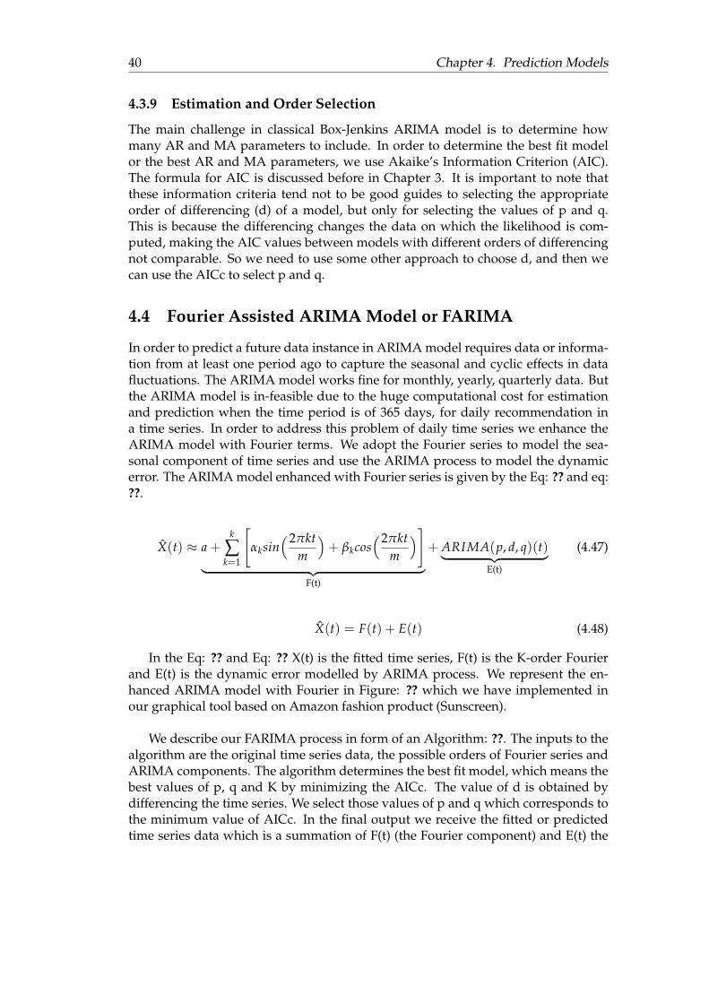
40 Chapter 4. Prediction Models
4.3.9 Estimation and Order Selection
The main challenge in classical Box-Jenkins ARIMA model is to determine howmany AR and MA parameters to include. In order to determine the best fit modelor the best AR and MA parameters, we use Akaike’s Information Criterion (AIC).The formula for AIC is discussed before in Chapter 3. It is important to note thatthese information criteria tend not to be good guides to selecting the appropriateorder of differencing (d) of a model, but only for selecting the values of p and q.This is because the differencing changes the data on which the likelihood is com-puted, making the AIC values between models with different orders of differencingnot comparable. So we need to use some other approach to choose d, and then wecan use the AICc to select p and q.
4.4 Fourier Assisted ARIMA Model or FARIMA
In order to predict a future data instance in ARIMA model requires data or informa-tion from at least one period ago to capture the seasonal and cyclic effects in datafluctuations. The ARIMA model works fine for monthly, yearly, quarterly data. Butthe ARIMA model is in-feasible due to the huge computational cost for estimationand prediction when the time period is of 365 days, for daily recommendation ina time series. In order to address this problem of daily time series we enhance theARIMA model with Fourier terms. We adopt the Fourier series to model the sea-sonal component of time series and use the ARIMA process to model the dynamicerror. The ARIMA model enhanced with Fourier series is given by the Eq: ?? and eq:??.
X(t) ≈ a +k
∑k=1
[αksin
(2πktm
)+ βkcos
(2πktm
)]︸ ︷︷ ︸
F(t)
+ ARIMA(p, d, q)(t)︸ ︷︷ ︸E(t)
(4.47)
X(t) = F(t) + E(t) (4.48)
In the Eq: ?? and Eq: ?? X(t) is the fitted time series, F(t) is the K-order Fourierand E(t) is the dynamic error modelled by ARIMA process. We represent the en-hanced ARIMA model with Fourier in Figure: ?? which we have implemented inour graphical tool based on Amazon fashion product (Sunscreen).
We describe our FARIMA process in form of an Algorithm: ??. The inputs to thealgorithm are the original time series data, the possible orders of Fourier series andARIMA components. The algorithm determines the best fit model, which means thebest values of p, q and K by minimizing the AICc. The value of d is obtained bydifferencing the time series. We select those values of p and q which corresponds tothe minimum value of AICc. In the final output we receive the fitted or predictedtime series data which is a summation of F(t) (the Fourier component) and E(t) the
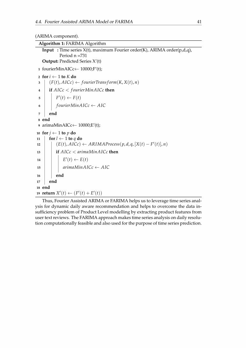
4.4. Fourier Assisted ARIMA Model or FARIMA 41
(ARIMA component).
Algorithm 1: FARIMA AlgorithmInput : Time series X(t), maximum Fourier order(K), ARIMA order(p,d,q),
Period n =731Output: Predicted Series X’(t)
1 fourierMinAICc← 10000;F’(t);
2 for i← 1 to K do3 (F(t), AICc)← f ourierTrans f orm(K, X(t), n)
4 if AICc < f ourierMinAICc then
5 F′(t)← F(t)
6 f ourierMinAICc← AIC
7 end8 end9 arimaMinAICc← 10000;E’(t);
10 for j← 1 to p do11 for l ← 1 to q do12 (E(t), AICc)← ARIMAProcess(p, d, q, [X(t)− F′(t)], n)
13 if AICc < arimaMinAICc then
14 E′(t)← E(t)
15 arimaMinAICc← AIC
16 end17 end18 end19 return X′(t)← (F′(t) + E′(t))
Thus, Fourier Assisted ARIMA or FARIMA helps us to leverage time series anal-ysis for dynamic daily aware recommendation and helps to overcome the data in-sufficiency problem of Product Level modelling by extracting product features fromuser text reviews. The FARIMA approach makes time series analysis on daily resolu-tion computationally feasible and also used for the purpose of time series prediction.
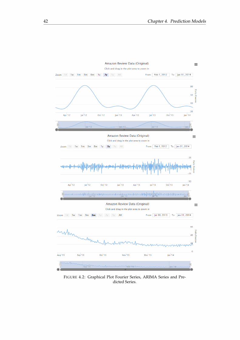
42 Chapter 4. Prediction Models
FIGURE 4.2: Graphical Plot Fourier Series, ARIMA Series and Pre-dicted Series.
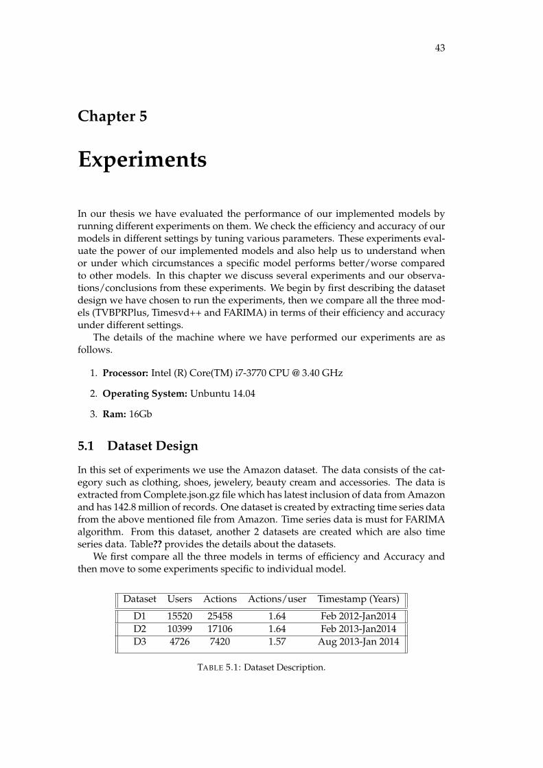
43
Chapter 5
Experiments
In our thesis we have evaluated the performance of our implemented models byrunning different experiments on them. We check the efficiency and accuracy of ourmodels in different settings by tuning various parameters. These experiments eval-uate the power of our implemented models and also help us to understand whenor under which circumstances a specific model performs better/worse comparedto other models. In this chapter we discuss several experiments and our observa-tions/conclusions from these experiments. We begin by first describing the datasetdesign we have chosen to run the experiments, then we compare all the three mod-els (TVBPRPlus, Timesvd++ and FARIMA) in terms of their efficiency and accuracyunder different settings.
The details of the machine where we have performed our experiments are asfollows.
1. Processor: Intel (R) Core(TM) i7-3770 CPU @ 3.40 GHz
2. Operating System: Unbuntu 14.04
3. Ram: 16Gb
5.1 Dataset Design
In this set of experiments we use the Amazon dataset. The data consists of the cat-egory such as clothing, shoes, jewelery, beauty cream and accessories. The data isextracted from Complete.json.gz file which has latest inclusion of data from Amazonand has 142.8 million of records. One dataset is created by extracting time series datafrom the above mentioned file from Amazon. Time series data is must for FARIMAalgorithm. From this dataset, another 2 datasets are created which are also timeseries data. Table?? provides the details about the datasets.
We first compare all the three models in terms of efficiency and Accuracy andthen move to some experiments specific to individual model.
Dataset Users Actions Actions/user Timestamp (Years)
D1 15520 25458 1.64 Feb 2012-Jan2014D2 10399 17106 1.64 Feb 2013-Jan2014D3 4726 7420 1.57 Aug 2013-Jan 2014
TABLE 5.1: Dataset Description.
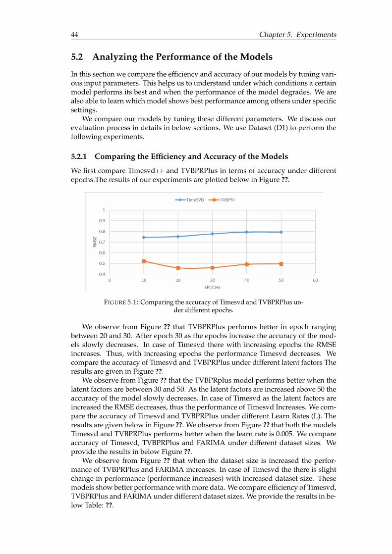
44 Chapter 5. Experiments
5.2 Analyzing the Performance of the Models
In this section we compare the efficiency and accuracy of our models by tuning vari-ous input parameters. This helps us to understand under which conditions a certainmodel performs its best and when the performance of the model degrades. We arealso able to learn which model shows best performance among others under specificsettings.
We compare our models by tuning these different parameters. We discuss ourevaluation process in details in below sections. We use Dataset (D1) to perform thefollowing experiments.
5.2.1 Comparing the Efficiency and Accuracy of the Models
We first compare Timesvd++ and TVBPRPlus in terms of accuracy under differentepochs.The results of our experiments are plotted below in Figure ??.
FIGURE 5.1: Comparing the accuracy of Timesvd and TVBPRPlus un-der different epochs.
We observe from Figure ?? that TVBPRPlus performs better in epoch rangingbetween 20 and 30. After epoch 30 as the epochs increase the accuracy of the mod-els slowly decreases. In case of Timesvd there with increasing epochs the RMSEincreases. Thus, with increasing epochs the performance Timesvd decreases. Wecompare the accuracy of Timesvd and TVBPRPlus under different latent factors Theresults are given in Figure ??.
We observe from Figure ?? that the TVBPRplus model performs better when thelatent factors are between 30 and 50. As the latent factors are increased above 50 theaccuracy of the model slowly decreases. In case of Timesvd as the latent factors areincreased the RMSE decreases, thus the performance of Timesvd Increases. We com-pare the accuracy of Timesvd and TVBPRPlus under different Learn Rates (L). Theresults are given below in Figure ??. We observe from Figure ?? that both the modelsTimesvd and TVBPRPlus performs better when the learn rate is 0.005. We compareaccuracy of Timesvd, TVBPRPlus and FARIMA under different dataset sizes. Weprovide the results in below Figure ??.
We observe from Figure ?? that when the dataset size is increased the perfor-mance of TVBPRPlus and FARIMA increases. In case of Timesvd the there is slightchange in performance (performance increases) with increased dataset size. Thesemodels show better performance with more data. We compare efficiency of Timesvd,TVBPRPlus and FARIMA under different dataset sizes. We provide the results in be-low Table: ??.
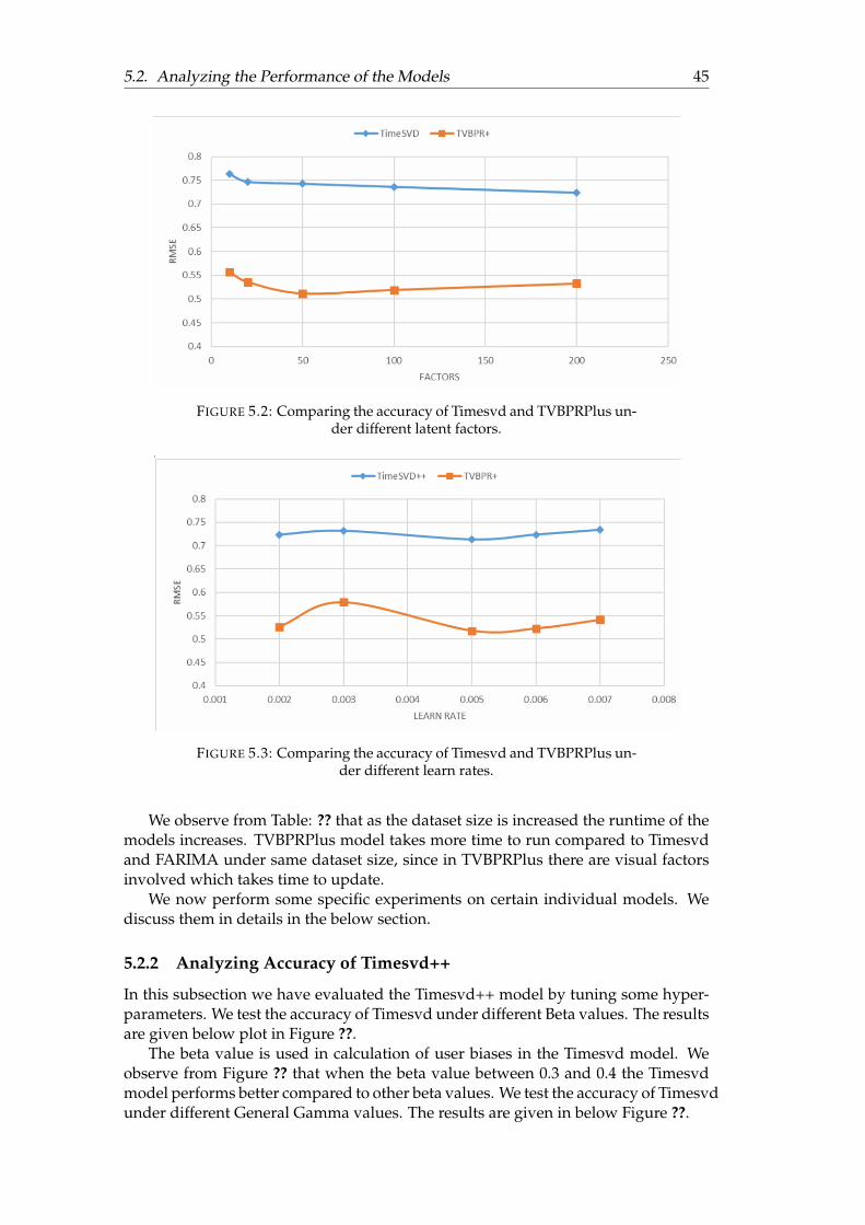
5.2. Analyzing the Performance of the Models 45
FIGURE 5.2: Comparing the accuracy of Timesvd and TVBPRPlus un-der different latent factors.
FIGURE 5.3: Comparing the accuracy of Timesvd and TVBPRPlus un-der different learn rates.
We observe from Table: ?? that as the dataset size is increased the runtime of themodels increases. TVBPRPlus model takes more time to run compared to Timesvdand FARIMA under same dataset size, since in TVBPRPlus there are visual factorsinvolved which takes time to update.
We now perform some specific experiments on certain individual models. Wediscuss them in details in the below section.
5.2.2 Analyzing Accuracy of Timesvd++
In this subsection we have evaluated the Timesvd++ model by tuning some hyper-parameters. We test the accuracy of Timesvd under different Beta values. The resultsare given below plot in Figure ??.
The beta value is used in calculation of user biases in the Timesvd model. Weobserve from Figure ?? that when the beta value between 0.3 and 0.4 the Timesvdmodel performs better compared to other beta values. We test the accuracy of Timesvdunder different General Gamma values. The results are given in below Figure ??.
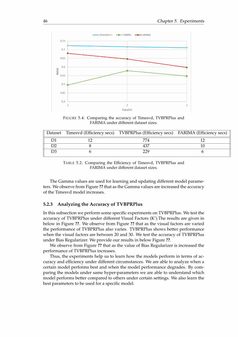
46 Chapter 5. Experiments
FIGURE 5.4: Comparing the accuracy of Timesvd, TVBPRPlus andFARIMA under different dataset sizes.
Dataset Timesvd (Efficiency secs) TVBPRPlus (Efficiency secs) FARIMA (Efficiency secs)
D1 12 774 12D2 8 437 10D3 6 229 6
TABLE 5.2: Comparing the Efficiency of Timesvd, TVBPRPlus andFARIMA under different dataset sizes.
The Gamma values are used for learning and updating different model parame-ters. We observe from Figure ?? that as the Gamma values are increased the accuracyof the Timesvd model increases.
5.2.3 Analyzing the Accuracy of TVBPRPlus
In this subsection we perform some specific experiments on TVBPRPlus. We test theaccuracy of TVBPRPlus under different Visual Factors (K’).The results are given inbelow in Figure ??. We observe from Figure ?? that as the visual factors are variedthe performance of TVBPRPlus also varies. TVBPRPlus shows better performancewhen the visual factors are between 20 and 30. We test the accuracy of TVBPRPlusunder Bias Regularizer. We provide our results in below Figure ??.
We observe from Figure ?? that as the value of Bias Regularizer is increased theperformance of TVBPRPlus increases.
Thus, the experiments help us to learn how the models perform in terms of ac-curacy and efficiency under different circumstances. We are able to analyze when acertain model performs best and when the model performance degrades. By com-paring the models under same hyper-parameters we are able to understand whichmodel performs better compared to others under certain settings. We also learn thebest parameters to be used for a specific model.
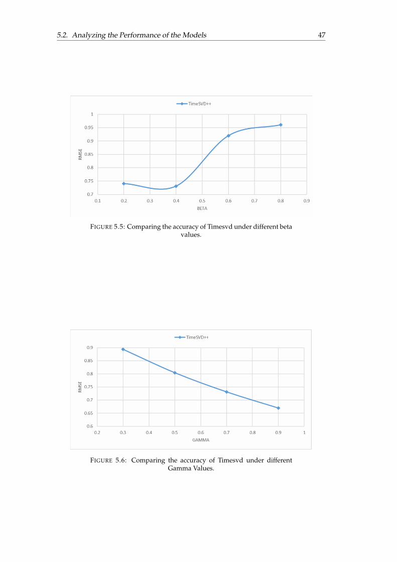
5.2. Analyzing the Performance of the Models 47
FIGURE 5.5: Comparing the accuracy of Timesvd under different betavalues.
FIGURE 5.6: Comparing the accuracy of Timesvd under differentGamma Values.
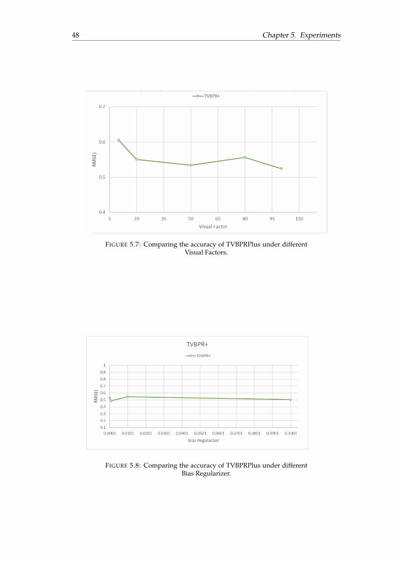
48 Chapter 5. Experiments
FIGURE 5.7: Comparing the accuracy of TVBPRPlus under differentVisual Factors.
FIGURE 5.8: Comparing the accuracy of TVBPRPlus under differentBias Regularizer.
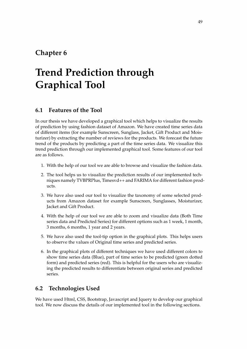
49
Chapter 6
Trend Prediction throughGraphical Tool
6.1 Features of the Tool
In our thesis we have developed a graphical tool which helps to visualize the resultsof prediction by using fashion dataset of Amazon. We have created time series dataof different items (for example Sunscreen, Sunglass, Jacket, Gift Product and Mois-turizer) by extracting the number of reviews for the products. We forecast the futuretrend of the products by predicting a part of the time series data. We visualize thistrend prediction through our implemented graphical tool. Some features of our toolare as follows.
1. With the help of our tool we are able to browse and visualize the fashion data.
2. The tool helps us to visualize the prediction results of our implemented tech-niques namely TVBPRPlus, Timesvd++ and FARIMA for different fashion prod-ucts.
3. We have also used our tool to visualize the taxonomy of some selected prod-ucts from Amazon dataset for example Sunscreen, Sunglasses, Moisturizer,Jacket and Gift Product.
4. With the help of our tool we are able to zoom and visualize data (Both Timeseries data and Predicted Series) for different options such as 1 week, 1 month,3 months, 6 months, 1 year and 2 years.
5. We have also used the tool-tip option in the graphical plots. This helps usersto observe the values of Original time series and predicted series.
6. In the graphical plots of different techniques we have used different colors toshow time series data (Blue), part of time series to be predicted (green dottedform) and predicted series (red). This is helpful for the users who are visualiz-ing the predicted results to differentiate between original series and predictedseries.
6.2 Technologies Used
We have used Html, CSS, Bootstrap, Javascript and Jquery to develop our graphicaltool. We now discuss the details of our implemented tool in the following sections.
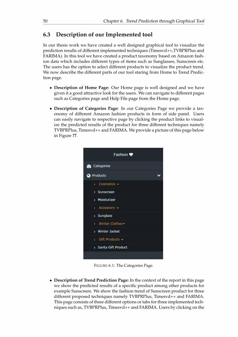
50 Chapter 6. Trend Prediction through Graphical Tool
6.3 Description of our Implemented tool
In our thesis work we have created a well designed graphical tool to visualize theprediction results of different implemented techniques (Timesvd++,TVBPRPlus andFARIMA). In this tool we have created a product taxonomy based on Amazon fash-ion data which includes different types of items such as Sunglasses, Sunscreen etc.The users has the option to select different products to visualize the product trend.We now describe the different parts of our tool staring from Home to Trend Predic-tion page.
• Description of Home Page: Our Home page is well designed and we havegiven it a good attractive look for the users. We can navigate to different pagessuch as Categories page and Help File page from the Home page.
• Description of Categories Page: In our Categories Page we provide a tax-onomy of different Amazon fashion products in form of side panel. Userscan easily navigate to respective page by clicking the product links to visual-ize the predicted results of the product for three different techniques namelyTVBPRPlus, Timesvd++ and FARIMA. We provide a picture of this page belowin Figure ??.
FIGURE 6.1: The Categories Page.
• Description of Trend Prediction Page: In the context of the report in this pagewe show the predicted results of a specific product among other products forexample Sunscreen. We show the fashion trend of Sunscreen product for threedifferent proposed techniques namely TVBPRPlus, Timesvd++ and FARIMA.This page consists of three different options or tabs for three implemented tech-niques such as, TVBPRPlus, Timesvd++ and FARIMA. Users by clicking on the
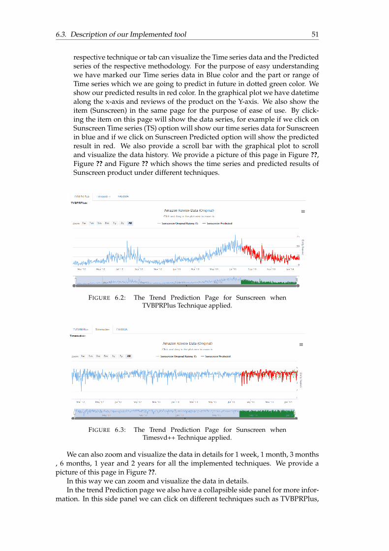
6.3. Description of our Implemented tool 51
respective technique or tab can visualize the Time series data and the Predictedseries of the respective methodology. For the purpose of easy understandingwe have marked our Time series data in Blue color and the part or range ofTime series which we are going to predict in future in dotted green color. Weshow our predicted results in red color. In the graphical plot we have datetimealong the x-axis and reviews of the product on the Y-axis. We also show theitem (Sunscreen) in the same page for the purpose of ease of use. By click-ing the item on this page will show the data series, for example if we click onSunscreen Time series (TS) option will show our time series data for Sunscreenin blue and if we click on Sunscreen Predicted option will show the predictedresult in red. We also provide a scroll bar with the graphical plot to scrolland visualize the data history. We provide a picture of this page in Figure ??,Figure ?? and Figure ?? which shows the time series and predicted results ofSunscreen product under different techniques.
FIGURE 6.2: The Trend Prediction Page for Sunscreen whenTVBPRPlus Technique applied.
FIGURE 6.3: The Trend Prediction Page for Sunscreen whenTimesvd++ Technique applied.
We can also zoom and visualize the data in details for 1 week, 1 month, 3 months, 6 months, 1 year and 2 years for all the implemented techniques. We provide apicture of this page in Figure ??.
In this way we can zoom and visualize the data in details.In the trend Prediction page we also have a collapsible side panel for more infor-
mation. In this side panel we can click on different techniques such as TVBPRPlus,
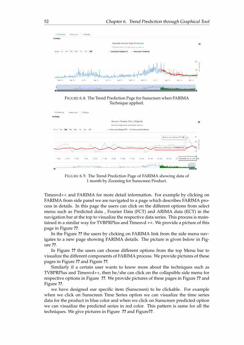
52 Chapter 6. Trend Prediction through Graphical Tool
FIGURE 6.4: The Trend Prediction Page for Sunscreen when FARIMATechnique applied.
FIGURE 6.5: The Trend Prediction Page of FARIMA showing data of1 month by Zooming for Sunscreen Product.
Timesvd++ and FARIMA for more detail information. For example by clicking onFARIMA from side panel we are navigated to a page which describes FARIMA pro-cess in details. In this page the users can click on the different options from selectmenu such as Predicted data , Fourier Data (FCT) and ARIMA data (ECT) in thenavigation bar at the top to visualize the respective data series. This process is main-tained in a similar way for TVBPRPlus and Timesvd ++. We provide a picture of thispage in Figure ??.
In the Figure ?? the users by clicking on FARIMA link from the side menu nav-igates to a new page showing FARIMA details. The picture is given below in Fig-ure ??.
In Figure ?? the users can choose different options from the top Menu bar tovisualize the different components of FARIMA process. We provide pictures of thesepages in Figure ?? and Figure ??.
Similarly if a certain user wants to know more about the techniques such asTVBPRPlus and Timesvd++, then he/she can click on the collapsible side menu forrespective options in Figure ??. We provide pictures of these pages in Figure ?? andFigure ??.
we have designed our specific item (Sunscreen) to be clickable. For examplewhen we click on Sunscreen Time Series option we can visualize the time seriesdata for the product in blue color and when we click on Sunscreen predicted optionwe can visualize the predicted series in red color. This pattern is same for all thetechniques. We give pictures in Figure ?? and Figure??.
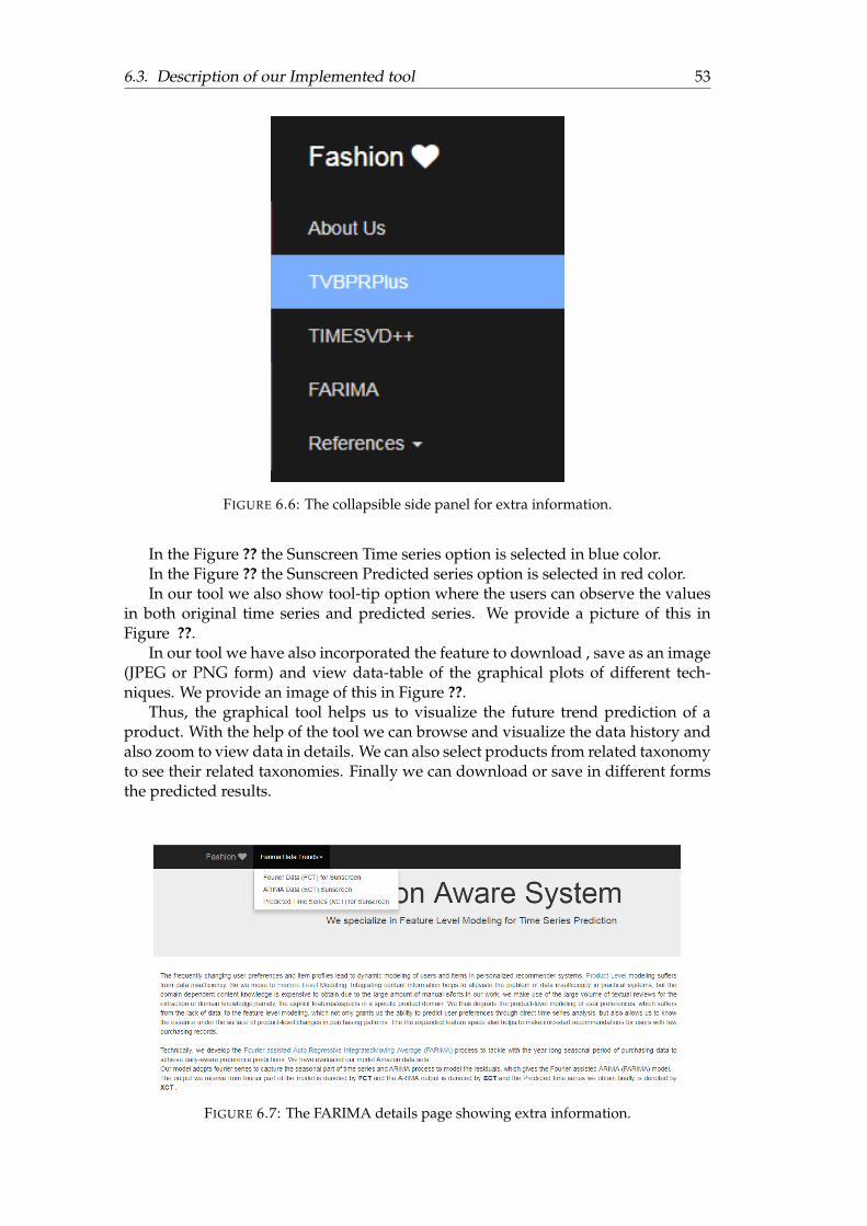
6.3. Description of our Implemented tool 53
FIGURE 6.6: The collapsible side panel for extra information.
In the Figure ?? the Sunscreen Time series option is selected in blue color.In the Figure ?? the Sunscreen Predicted series option is selected in red color.In our tool we also show tool-tip option where the users can observe the values
in both original time series and predicted series. We provide a picture of this inFigure ??.
In our tool we have also incorporated the feature to download , save as an image(JPEG or PNG form) and view data-table of the graphical plots of different tech-niques. We provide an image of this in Figure ??.
Thus, the graphical tool helps us to visualize the future trend prediction of aproduct. With the help of the tool we can browse and visualize the data history andalso zoom to view data in details. We can also select products from related taxonomyto see their related taxonomies. Finally we can download or save in different formsthe predicted results.
FIGURE 6.7: The FARIMA details page showing extra information.
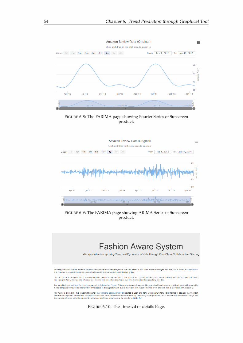
54 Chapter 6. Trend Prediction through Graphical Tool
FIGURE 6.8: The FARIMA page showing Fourier Series of Sunscreenproduct.
FIGURE 6.9: The FARIMA page showing ARIMA Series of Sunscreenproduct.
FIGURE 6.10: The Timesvd++ details Page.
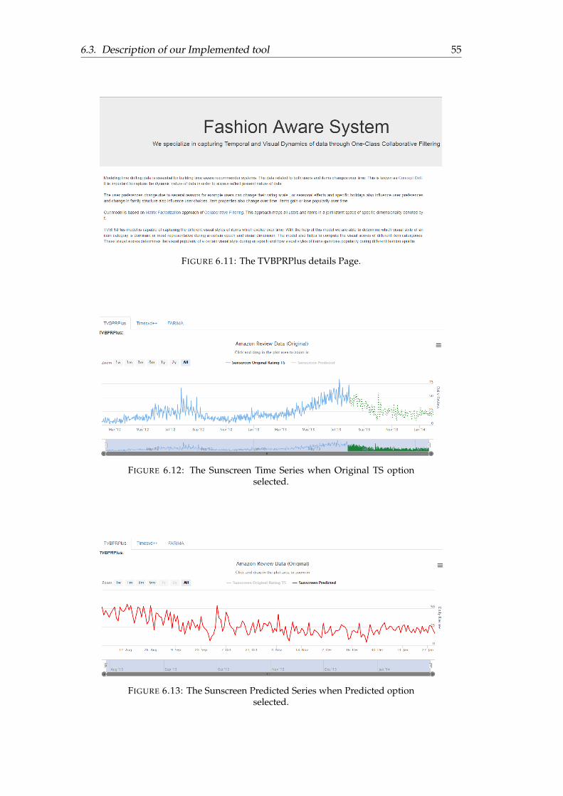
6.3. Description of our Implemented tool 55
FIGURE 6.11: The TVBPRPlus details Page.
FIGURE 6.12: The Sunscreen Time Series when Original TS optionselected.
FIGURE 6.13: The Sunscreen Predicted Series when Predicted optionselected.
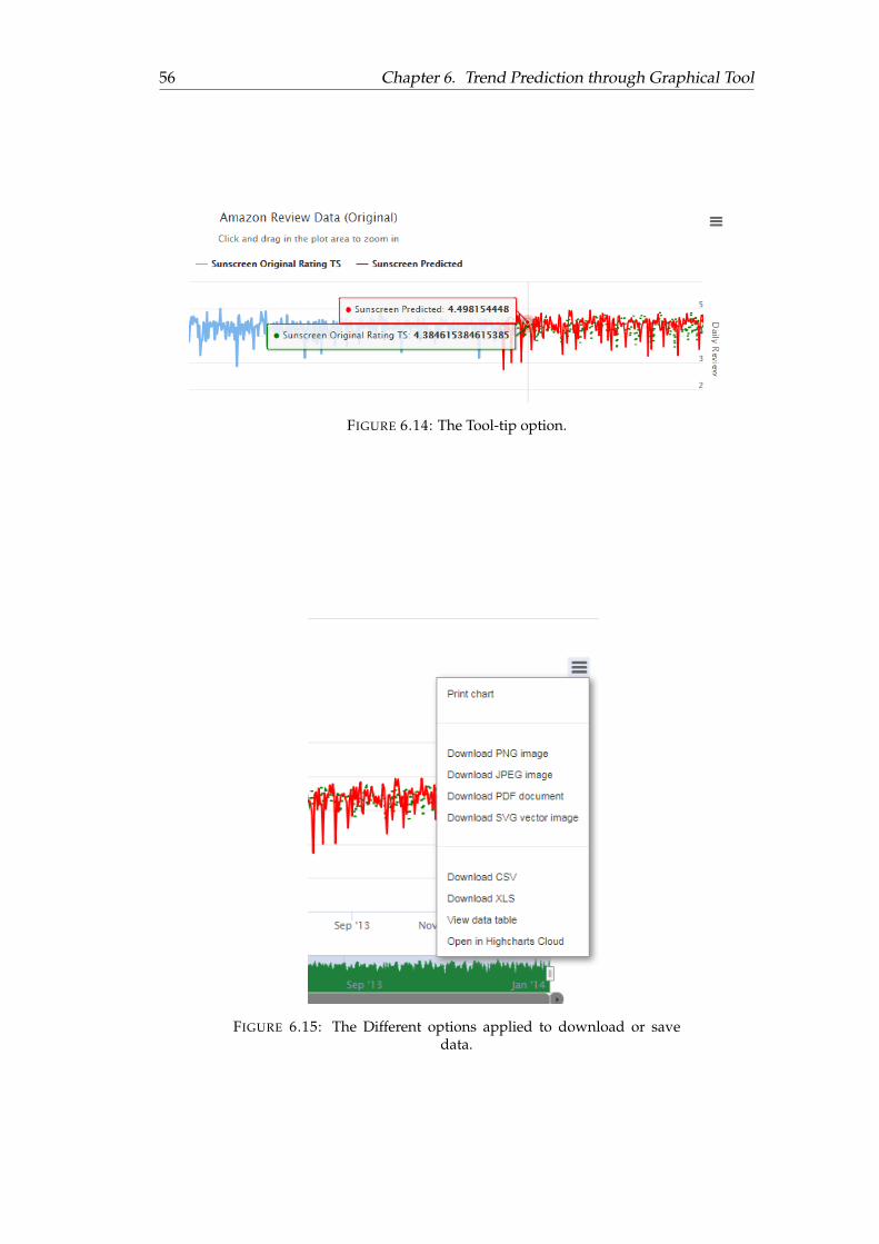
56 Chapter 6. Trend Prediction through Graphical Tool
FIGURE 6.14: The Tool-tip option.
FIGURE 6.15: The Different options applied to download or savedata.
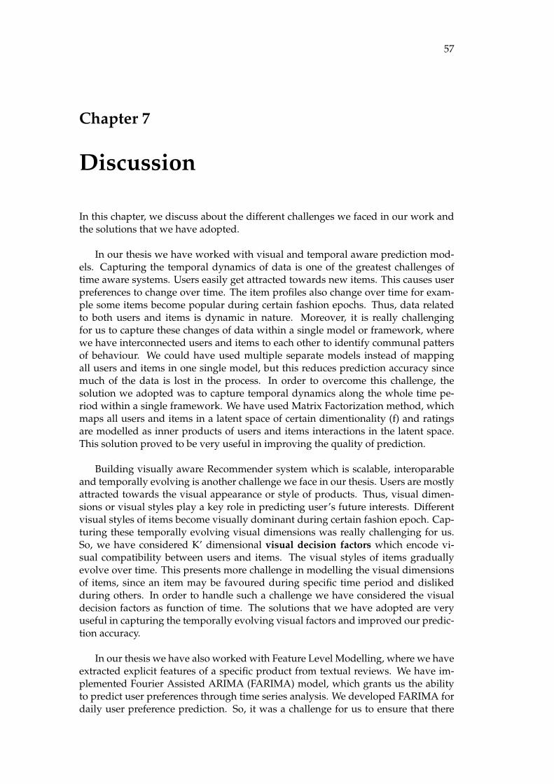
57
Chapter 7
Discussion
In this chapter, we discuss about the different challenges we faced in our work andthe solutions that we have adopted.
In our thesis we have worked with visual and temporal aware prediction mod-els. Capturing the temporal dynamics of data is one of the greatest challenges oftime aware systems. Users easily get attracted towards new items. This causes userpreferences to change over time. The item profiles also change over time for exam-ple some items become popular during certain fashion epochs. Thus, data relatedto both users and items is dynamic in nature. Moreover, it is really challengingfor us to capture these changes of data within a single model or framework, wherewe have interconnected users and items to each other to identify communal pattersof behaviour. We could have used multiple separate models instead of mappingall users and items in one single model, but this reduces prediction accuracy sincemuch of the data is lost in the process. In order to overcome this challenge, thesolution we adopted was to capture temporal dynamics along the whole time pe-riod within a single framework. We have used Matrix Factorization method, whichmaps all users and items in a latent space of certain dimentionality (f) and ratingsare modelled as inner products of users and items interactions in the latent space.This solution proved to be very useful in improving the quality of prediction.
Building visually aware Recommender system which is scalable, interoparableand temporally evolving is another challenge we face in our thesis. Users are mostlyattracted towards the visual appearance or style of products. Thus, visual dimen-sions or visual styles play a key role in predicting user’s future interests. Differentvisual styles of items become visually dominant during certain fashion epoch. Cap-turing these temporally evolving visual dimensions was really challenging for us.So, we have considered K’ dimensional visual decision factors which encode vi-sual compatibility between users and items. The visual styles of items graduallyevolve over time. This presents more challenge in modelling the visual dimensionsof items, since an item may be favoured during specific time period and dislikedduring others. In order to handle such a challenge we have considered the visualdecision factors as function of time. The solutions that we have adopted are veryuseful in capturing the temporally evolving visual factors and improved our predic-tion accuracy.
In our thesis we have also worked with Feature Level Modelling, where we haveextracted explicit features of a specific product from textual reviews. We have im-plemented Fourier Assisted ARIMA (FARIMA) model, which grants us the abilityto predict user preferences through time series analysis. We developed FARIMA fordaily user preference prediction. So, it was a challenge for us to ensure that there
58 Chapter 7. Discussion
is no discontinuity in time series data. In order to tackle this challenge we collectedall the dates (time) and the corresponding number of reviews for each data for aparticular feature and sorted our data (Both dates and reviews) to make sure thatno data is missing. Thus, we prepared a continuous time series (TS) of 2 years fora particular product feature. It is very important and challenging to make the timeseries stationary over time for future predictions. So, we have differentiated ourtime series data and plotted it to ensure that all the trends are removed and the timeseries is stationary over time. Estimating the correct order of parameters such ascorrect Fourier order or AR/MA orders was also a challenging job. In order to se-lect the best fit model we have used the evaluation technique according to the paper[Zhang0ZLLZM15] known as Akaike’s Information Criterion (AICc). The solutionswe adopted helped us to estimate the best fit model and determine the future trendof the product.
Apart from the above challenges we have also faced some technical challenges.In our thesis we have implemented our prediction models in Java language. In thefirst two models such as TVBPRPlus and Timesvd++, we have considered Java Ar-rays to represent certain model parameters in our code. But while running the codeto generate predicted results we found there was efficiency and memory problems.So, later we replaced those parameters with Java ArrayList to solve the problem. Re-garding the FARIMA model we also faced some technical problems such as it couldbe much easier for us to implement FARIMA in languages like R instead of Java,since in R language we already have in-built packages for ARIMA process. But inour case we tried to understand the underlying concepts of FARIMA in details. Thenwe have implemented the different components of the model programatically with-out the use of in-built packages. In our graphical tool we have visualized the futuretrend of a specific product. This can be easily achieved for FARIMA model. But foruser centric models like TVBPRPlus (ranking based) and Timesvd++ (rating based)this was challenging. So, we have adopted our models in such a way so that we cancompare all the models on a common ground and visualize the trend prediction ofa specific product. For example in case of Timesvd++ we have considered the num-ber of product reviews to determine its future trend. In case of TVBPRPlus we haveconsidered the number of reviews of a certain product known to the user to predictthe future trend of the product or similar products that can be recommended to theuser.
59
Chapter 8
Conclusion
Fashion is a fascinating domain that have gained a lot of attention due to the emer-gence of new products in the market. The main focus of our thesis was to implementthe three prediction models namely TVBPRPlus,Timesvd++ and FARIMA based onAmazon fashion data and design a graphical tool that visualizes the prediction re-sults of these techniques.In our thesis work we have developed time and visuallyaware Recommender systems such as TVBPRPlus and Timesvd++ based on userfeedback and product images (Product Level Modelling). Our models are capable ofcapturing evolving visual dimensions of products and as well as associated tempo-ral dynamics of data. We have applied these models to determine the future trend ofa certain item (Sunscreen product). We have also developed Recommender systemsbased on Feature Level modelling (Fourier Assisted ARIMA or FARIMA), where wehave extracted explicit features of a specific product. FARIMA helps us to achievedaily aware preference prediction through time series analysis. We have designed agraphical tool to visualize the predicted results of these different models.
In order to see the power of the models we have evaluated them using differ-ent evaluation techniques. We have compared the efficiency and accuracy of thesemodels by changing the different input parameters. We have learned which modelperforms better than others in certain settings and what should be the ideal valuesof the model parameters to achieve best performance from a specific model.
60
Chapter 9
Future Scope
In our work we have used feature level modelling in FARIMA model. We haveextracted explicit features from user reviews for a particular product domain. Thefeature extraction is done by Keyword search from user reviews. In future we planto perform feature extraction through an automatic tool. The feature extraction toolwill perform data pre-processing, tokenization and data parsing to extract featuresfrom textual reviews. In case of TVBPRPlus model we have determined visuallysimilar items among top 50 items and found the future visual popularity of one spe-cific item based on their visual scores in the experimental section. We plan to includethis concept as a part of our graphical tool which will show the similar products inthe visual space.

Chapter 9. Future Scope 61
[HeM16] [Koren10] [VBPR] [Zhang0ZLLZM15] [Al-HalahSG17] [Fashionista][MelvilleS17] [BPR] [KorenBV09] [TSForecast]