A Work Project, presented as part of the requirements for the Award of a Masters

Degree in Finance from the Faculdade de Economia da Universidade Nova de Lisboa

TREASURY BOND RETURNS AND U.S. POLITICAL CYCLES

CARLOS MIGUEL SILVA FREIXA

(MASTERS IN FINANCE Nº86)

A Project carried out with the supervision of:

Prof. João Amaro de Matos

Lisboa, 12th June 2009

2

2

TREASURY BOND RETURNS AND U.S. POLITICAL CYCLES

Abstract

This work-project complements the existing studies on the linkage between financial

investments returns and the political cycles, by relating Treasury bond returns and

Presidential cycles. Previous research shows that stock market tends to behave better

during Democratic presidencies, and in this work it is shown a compatible result, with

long-term Treasury bonds having higher absolute, and excess returns during Republican

Administrations. This difference is not explained by business cycles and there are no

significant differences in risk, as measured by the volatility of returns, between the two

political cycles. Empirical evidence is also found showing that there are better economic

and financial conditions to invest in T-bonds' markets during Republican than during

Democratic Administrations.

Keywords: Treasury Bond Returns, Political Cycles, Political Economy

3

3

TREASURY BOND RETURNS AND U.S. POLITICAL CYCLES

I - Introduction

This work-project provides evidence about the relationship between the Treasury

bond returns and the political cycles in the United States. The influence of political and

Presidential cycles in the capital markets returns is a considerable aspect since both

Republicans and Democrats have different ideas and pursue different policies. These

differences affect directly the financial market returns, not only by different economic

and financial measures but also with different law revisions. On the other hand, there

can also be other line of thought, in which policies followed by Presidents are not so

different, and when elected, the President and the majority in power will have the

tendency to adopt strategies and measures that might help a future re-election, and so

financial returns should be totally independent from political variables. Despite this last

hypothesis, Treasury bond returns are largely connected with the monetary and fiscal

policies adopted by Governments, because they directly influence interest rates, and

consequently bond markets. The differences between the two ideologies are known,

whereas Democratic Administrations are expected to follow expansionary policies with

more public sector intervention and employment stimulation, alternatively, Republican

Administrations normally pursue the lowering of taxes, interest rates and inflation. So,

these different approaches should have a direct impact in public expenditures, public

debt level, Gross Domestic Product, inflation and interest rates level that ultimately

influence Treasury bond returns. The purpose of this study, as stated before, is to

analyze empirically the differences in political cycles of returns and from that

extrapolate what are the “best” regimes for investors to increase the weight of

Government bonds in their portfolio allocations.

4

4

The economic environment that offers better conditions to invest in Bonds, is

generally the economic state with low inflation and low interest rates, because it lowers

the opportunity cost of investing in bonds, making coupon payments more attractive

relatively to interest rate remunerations. Historically, in the 20th Century, there were

periods in which the conditions were favorable to invest in bonds, like the last 20 years

of the last century, and the beginning of the 2000’s, with low interest rates and low

inflation. On the contrary, since the end of the World War II and the beginning of

1980’s there were periods with high inflation, and with high interest rates with

instability in debt markets, creating then a bear market for fixed income investments.

Long-term bonds are important and are held by investors mainly for two reasons: they

are good instruments to assume long-term hedging positions, and also this type of

bonds, normally, has a premium over short-term investments, and this premium can be

used for speculative motives.

This work is organized as follow, firstly it is presented the literature review with

the description of similar findings by previous research, afterwards data and

methodology description with explanation of main results. The results are then

compared with tests in subsamples using additional robustness statistical tests. It is also

analyzed whether the excess returns differences are due to different risk assumed in the

two cycles. This will be accessed estimating the volatilities of returns in the two parties’

cycles. Finally, some limitations of the work-project are presented, as well as alternative

methodologies, and further research topics.

Literature Review

There are not many studies showing the relationship between bond returns and

political cycles. However, the relationship of stock returns and Presidency cycles is

5

5

widely approached in different papers, like Hensel and Ziemba (1995) who study the

returns between small and big caps during both administrations, finding that during

Democrats, indifferently of cap size, stock returns are significantly higher. In a more

recent study performed by Santa Clara and Valkanov (2003), the authors reach similar

conclusions. Using CRSP value weighted index returns as proxy for monthly stock

market returns, from 1929 to 1998, they find that during Democrat Administrations,

excess returns on the stock market are much higher compared with Republicans.

Interestingly they also find that the risk is higher during Republican cycles, so the excess

return is not a compensation for higher risk, constituting in this way a puzzle. From a

macroeconomic point of a view, and using similar methodology, Elliot (2006), in his

working-paper finds that from 1949 to 2005 real GDP growth is 5,1 percent in average

during Democratic Administrations, which is more than the double from Republicans

1,9 percent. For real GDP per capita the results are similar. He also tested whether the

effect of Congress was higher on GDP compared with the effect of Presidential

Administrations, because it is the Congress that decides on law material and approves

the Government budgets. The impact of Congress in GDP was not statistically different

from zero, so he concludes that the party in the Administration works as a better

explanatory variable for political cycles. From all, the most recent study is from

Ramchander Simpson and Webb (2008), in which they demonstrate the relationship of

Real Estate Investment Trusts (REIT) returns and political cycles. Contrary to the

previous results on the above cited papers, the authors find that the REIT excess returns

are much higher during Republican presidencies. The result is still significant when they

control for the monetary policy, using for control a dummy variable defining the

expansionary or loosening monetary policy, depending on the FED decision of lowering

6

6

or increasing interest rates. They also conclude that the evolution of these returns is

much higher during the two last mandate years specially for Republican mandates. The

importance of political gridlock, defined as the control of the majority of Congress,

Senate and Presidency is also studied, and the authors find that political gridlock

controlled by the same party helps the REIT returns, being these returns higher again

during Republican leaderships in all parts of the gridlock, independent from tightening

or loosening monetary policy. Wrapping up, all these papers present recent studies on

the relation of political variables with the economic and financial conditions. The goal

of this study is to complement the research presented, using different financial returns,

but with similar methodology, testing also the inferred conclusions, while adding more

updated results.

II - Data and Methodology

To examine the difference between returns on Treasury bonds along with

presidencies, it will be carried out a mean-variance approach using an OLS regression

with dummy variables. This regression is computed using the long term Treasury bonds

total returns (LTR), but also with excess returns on three month Treasury bill and

inflation. The first and principal regression specification is:

tttt eRPDMLTR ++= −− 1211 ββ (1)

The variable LTR stands for the returns on long-term Treasury bonds, and RP

and DM are the constructed dummy variables, in which RP assumes 1 if on that quarter

is a Republican President and 0 if it is Democratic, while DM assumes exactly the

opposite values. The coefficients for β1 and β2 correspond to the average returns for

Democrats and Republicans respectively. The explanatory variable is lagged, because

the political decisions are expected to influence interest rate markets with some delay.

7

7

This methodology only captures the evolution of the total returns in absolute

form, but for a more precise analysis, the evolution of excess returns should be

investigated. One can apply the same equation to the two types of excess returns

defined, first with excess returns on three month Treasury bill:

ttttt eRPDMTBLLTR ++=− −− 1211 ββ (2)

and secondly excess returns calculated over inflation:

ttttt eRPDMINFLTR ++=− −− 1211 ββ (3)

These three equations presented provide the starting and principal results for the

analysis, because, in case of having differences in these values, there is an historically

disparity between Republicans and Democrats. After these regressions, other tests are

performed to increase the robustness of the previous results. Using the same

methodological approach as before, tests can be made to sub-samples to confirm the

previous results, and at the same time helping to distinguish and find possible different

trends within the overall sample.

The list of Presidents was obtained from the White House web page, and for

cycle definition it was assumed that the presidential cycles started at the signature day.

In case of the existence of two presidents in the same quarter, it was assumed that the

person with more time within the quarter ran the entire quarter. The cycle could also be

defined with the election date, yet, for this type of returns, the difference in cycle

definitions is too small to produce considerable changes in interest rate markets and

influence final results. The main quantitative variables used are LTR, TBL, and INF,

and all of them were obtained from the database available at Prof. Amit Goyal webpage.

LTR is based on the Ibbotson Yearbook series; TBL is based in NBER macro history

8

8

data base until 1933, and from 1933 to 2007 it is obtained from the Federal Reserve

Bank at St. Louis (FRED); INF is retrieved from Consumer Price Index (All urban

Consumers) from the Bureau of Labor Statistics. The statistical descriptions,

Presidential cycles definition, and Dummy Variable descriptions are present in

Appendix - Table 1, Table 2 and Table 3.

III – Main Findings

a) Overall Results

Using the full sample of quarterly returns, since 1926 to 2008, in which there are

169 quarters with Democrat presidency and 159 for Republican presidencies, there are

high differences in long term Treasury bond returns between Democrats and

Republicans. The average return for Republican presidencies is 1,969 percent per

quarter, twice as much as for Democrat presidencies, which have 0,849 percent per

quarter in average. This implies that the average per year during Republican

Administrations is 7,876 percent and during Democratic Administrations is 3,360

percent. This is in line with what was expected ,because Democratic presidencies are

linked with more inflation and higher GDP growth, and on the other hand Republicans

prefer low inflation and lower interest rates and taxes, which favor the investment on

bonds. The difference of the two values being equal to zero is rejected, so there is

statistical evidence for high differences on the returns between the two parties. This

disparity is even higher when the difference between the excess returns over three

month T-bill is verified. In this test, during Democratic cycles the quarterly return was

0,105 percent (0,42 percent per year), and these values are not statistically different from

zero, while Republicans have 0,834 percent on a quarterly basis (3,33 percent per year).

Once again, statistically, the two averages are different from each other, but the

9

9

quarterly standard deviations of the coefficients are quite similar, 0,315 percent for

Democrats and 0,357 percent for Republicans on a quarterly basis. As to excess returns

on inflation, the results are again higher in Republican Administrations, because both

average returns are statistically different from zero, and Republicans present 1,830

percent (7,320 percent annually), and Democrats present 0,606 percent (2,424 percent

annually). All the values presented, statistical tests, and computational definitions for

regressions are presented in Appendix – Table 4.

In conclusion, there is statistical evidence that the Treasury bond returns are

different within political cycles. With this outcome, investors directly or indirectly see in

Republican presidencies conditions to add more financial gains to their bond

investments. Normally, Government debt is seen as riskless, or at least as a financial

investment with less risk. However, it is possible that differences in returns may be just

a consequence of the increased risk from Republican presidencies. Other feasible

explanation to the differences found is the type of policies followed by the governments.

In this case the party in power is really important to the investor’s decision, considering

that these policies have different consequences depending on the investments and

investor types. While the impacts of the political decisions on stock markets can affect

market prices more rapidly (for instance news about different government actions can

have an anticipated impact on stock indexes), on the other hand, the decisions on

Government debt emissions, interest rates fixation, and inflation control policies, which

are more likely to affect fixed income investors, have a much slower impact on debt

market prices. Finally, results are coherent to the economic premises and with previous

research on similar subjects.

10

10

b) Tests in subsamples

As stated above, to consign more assurance to the overall results, tests in sub-

samples will be executed in order to confirm the evolution of results in different

periods. The overall sample was divided in two subsamples, the first one ranges from

1926:Q1 to 1961:Q4, which translates into 144 observations after adjustments, with 82

quarters for Democrats and 61 quarters for Republicans. The second sub-sample ranges

from 1962:Q1 to 2007:Q4, including 184 observations, with 76 quarters for Democrats

and 108 quarters with Republicans in presidency. This division is set to split the sample

in two parts, according to different periods in the 20th century, because while the first

has significant history and economic marks like 1929 Depression, the World War II, and

the Economic Boom of the 50’s, the second subsample is more stable, with only the

Vietnam war as a significant U.S. historical mark. Naturally, there were also some

important shocks, like the oil shocks and the Cold War, but it was a period with higher

economic growth and with characteristics that favored the investment in financial assets.

For the first sub-sample and starting with the long-term Treasury bond returns,

Republican Administrations still present higher average returns, 0,921 percent (3,0684

percent) compared with 0,724 percent (2,896 percent annually) on Democratic

Administrations. Yet, these averages are statistically not different from each other, and

so, there were no real differences in long-term returns in this period. For the second sub-

sample, the difference not only is statistically different from zero, but also the behavior

of long-term bonds returns during Republican presidencies is exceedingly positive. For

Republicans the returns in this period were 2,576 percent (10,304 percent annually),

while for Democratic Presidencies it is only 0,982 percent (3,928 percent annually). It is

11

11

during this second period that the major difference between the two parties is

established.

Regarding excess returns on T-bill, one surprising result happens in the first sub-

sample. Unlike in total returns analysis, Democrats have higher excess returns on short-

term T-bill from 1926 to 1961. In this period the average for Republicans cycles is 1,264

percent per year, while for Democrats is 2,272 percent per year. This is the only time in

all analysis that the difference in returns was higher during Democrat cycles, but

statistically, both averages for the two parties are not different from zero. In the second

sub-sample, Republican cycles present a very good excess return on short-term T-bill,

with 1,134 percent (4,536 percent annually), and Democrat cycles had a negative return

with –0,387 percent (-1,548 percent annually). Though, this last value is not statistically

different from zero, which is in line with the overall results for the excess returns on T-

bill. As to excess returns on inflation, the results once again are in line with the results

obtained until now. In the first subsample, there is a difference of –0,521 percent

between the two average returns that is not statistically different from zero. The results

change in the second sub-sample because the quarterly difference is now –1,577 percent,

a value that is statistically different from zero, so once again Treasury bond returns are

higher during Republican presidencies. Concluding, tests in sub-samples attested

generally the overall result using periods with different economic conditions that could

influence the results. The major conclusion is that the source of the difference in returns

is more established in the second part of the century. In the first part there were

differences in returns but were not very high or statistically meaningful. The second part

of the analyzed period favored more investors, which had a debt market with more

12

12

liquidity, more debt issuing, and other conditions favorable to the investment in fixed

income securities, allowing to highlight the discrepancy in returns during Presidencies.

c) Tests Using Other Control Variables

On the results presented until now, it is assumed that political cycles are

independent from returns. However, returns may be correlated with other variables that

can also influence the presidency cycles. To manage this possibility, variables that can

impact on returns, should be controlled. In literature review, studies were presented

showing that GDP growth is different during the two administrations with economic

growth being much higher during Democrat presidencies. Taking this result in

consideration, the evolution of returns may be correlated with economic growth,

implying that the party in power might not directly affect returns. Also, different fiscal

policies and Government expenditure decisions can alter the size of debt issued by

Governments, and consequently impact on prices and bond returns. To control for

economic growth, and expenditures it will be used quarterly real GDP growth, and

Government expenditures growth, respectively. Both variables were obtained from the

Federal Reserve Economic Data (FRED) databases. Statistical description is available in

Appendix – Table 1. Both variables are quarterly, however there is only data available

starting 1947:Q3, so for the first 20 years, the impact of these variables will not be

measured. The methodology used will be similar as before, and the regressions will be

equal to equation (1), (2) and (3), but adding controls for GDP and Government

expenditures:

tttttt eEXPGDPRPDMLTR ++++= −−−− 12111211 ααββ (4)

ttttttt eEXPGDPRPDMTBLLTR ++++=− −−−− 12111211 ααββ (5)

13

13

ttttttt eEXPGDPRPDMINFLTR ++++=− −−−− 12111211 ααββ (6)

These equations will only be tested for two samples: first using all the new

variables sample, 1947:Q3 to 2007:Q4, and next using the second sample, 1962:Q1 to

2007:Q4. It is also in this second sample that previous results presented the major

differences between the two parties, so the impact of these variables on final results, if

significant, should be more meaningful in this sub-sample. Even when adding these two

new control variables, results on the second sub-sample are very similar to the initial

regressions, despite a small widening of the gap for the returns and excess returns on T-

bill. Regarding excess returns on inflation, the difference decreases (-1,35 percent

compared with –1,57 percent) but it is still significant. Finally GDP growth and Public

expenditures growth are not statistically significant in all equations, so these variables

do not have great impact on the explanation of long-term Treasury bond returns. Even

so, controlling for these variables can be helpful to eliminate possible correlation

between Presidency cycles and economic performances. However as seen before, the

overall conclusions are not modified and there is even more assurance that the main

results encountered before are indeed considerable.

Additionally other set of variables could be used to attest the conclusions, like

the level of monetary aggregates, yield spreads, or other possible macroeconomic

variables. Notwithstanding, the variables used in this work to control for financial and

economic influence, directly or indirectly are related with other possible explanatory

variables, and ultimately one is controlling for the other possible variables. Furthermore,

by adopting excess returns over inflation, the influence of macroeconomic factors is

previously eliminated, and the same logic applies to excess returns over T-bill for

monetary policy factors.

14

14

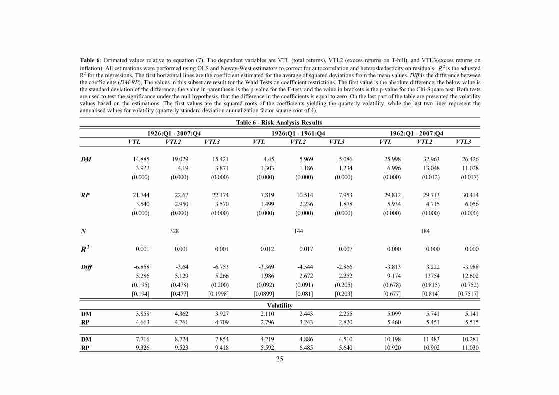
d) Return and Risk

Santa Clara and Valkanov in their work test for differences in risk during both

Administrations since one of the possible explanations for higher excess returns on

stock markets encountered is the higher risk assumed from investors, meaning that the

stock investors perceive Republicans as more risky than Democrats. This possible

explanation also holds for Government bond markets, and the result can also be justified

by the level of interest rates, which is normally lower during Republicans, but still not

withdrawing the possibility of having a risk premium embedded in the excess of returns.

To measure the risk difference between the two parties, it will be used the same

methodology as before, but in this case the dependent variable is the squared root of the

difference of to average of total returns on long term Treasury bonds. So the regression

held is:

tttt eRPDMVLT ++= −− 1211 ββ (7)

with:

2_____

−= LTRLTRVLT tt

This methodology was also applied to excess returns on T-bills and inflation.

With the results of this equation, a standard deviation for the returns can be calculated,

because, the dummy variable gives the average of the squared deviations from the mean,

which is the variance. Volatility, measured as the standard deviation is the squared root

of the estimated dummy. The results show that there are not significant differences in

risk, because the squared root differences from the average deviations are not

statistically different from each other. Even so, the calculated standard deviation of

returns are higher in Republican mandates for the three types of returns. However the

difference is not very high, and specially in the last part of the sample, differences in

15

15

volatility are very similar. Despite being an apparent evidence for higher volatility

during Republican presidencies, when analyzed the period where differences in returns

are higher, the volatilities estimations are not different from each other. This implies

that the market does not anticipate a premium over Republican presidencies, and

differences in risk are not the source for return discrepancy. The estimated results, data,

and methodology are described in Annex – Table 6.

e) Relationship between Stock Market Returns and Long-Term Bond Returns

Whenever stock markets are not good investments, common sense states that

investors should be driven to others more secure and return-safer, preferentially

Treasury bonds. As mentioned before, it is showed empirically in other papers that stock

markets behave better during Democratic presidencies, and in this work is shown that

returns on T-bonds are in average better during Republican administrations. The results

obtained in this paper are then coherent with previous research of the subject but using

different assets. It must not be forgotten that stocks and bonds are driven by different

factors other than political variables. Stocks normally follow earnings expectations, and

company’s performances that are more related to the economic cycles, while bonds are

more dependent on the monetary side, inflation and monetary levels. Using the LTR,

and the CRSP index as proxy for stock market risks, the correlation coefficient between

long-term returns and stock market is 0,119. Even with a low value, correlation is

positive. So historically there is a positive correlation between long-term bond returns

and stock market returns, which is not conclusive for the hypothesis of negative relation

between the two types of returns.

16

16

f) Limitations of this work and Further Research

Returns are a measure and depend on many factors. In this work it is

investigated whether long term Treasury bond returns were different within the political

cycles, using the long-term returns defined as in Ibbotson series. But, there are short-

term and long-term investors, and these results can vary for instance, if the holding

period of the bond changes, or if the investment horizon and risk aversion are different

from investor to investor. The variables chosen to justify this work are adequate and

consistent, but there are also other aspects linked with monetary policy and the financial

system that can matter to the analysis, for example, the person who runs the Federal

Reserve (FED) and consequently the monetary policy. However, the objective of this

work was to investigate if in both Republican and Democrat presidencies the return

averages were different, and not to analyze every aspect that could influence the return

on Government bonds.

The methodology used in this work is actually very simple. Using regressions

which only take dummy variables to distinguish the different political impacts on

returns, and controlling for other variables that might influence shifts in returns, these

equations help obtain good results for the proposed subject. Some robustness tests were

performed assuming different samples, and other explanatory variables. Nevertheless,

there can also be some problems with this methodology, because in this case the test

assumes that the dummy variable is constant over the sample, and the significance tests

applied to this value are subjected to this hypothesis. Though, it is possible to have

changes in the level of the dummy that are not influenced only by political tests,

implying that the conclusions about the significance of the political dummies could be

wrongly taken. This might be corrected by adding more control variables to justify the

17

17

changes in level of the dummies. In this work two were used (GDP and Government

expenditures growth), but there are other variables that perhaps should be included, and

omitting them can lead to erroneous results. The use of dummy variables to capture the

effect of political cycles is not broadly accepted, and for instance there are different

methodologies defended by Caporale and Gried (2005). To overcome this problem of

unexplained jumps in the series wrongly attributed to the political variables, they present

tests based on Bai and Perron methods, identifying the break points and the structural

changes in the intercepts, applying then different confidence intervals for the

significance tests on the dummy variables. There are also other critiques to the use of

dummy variables to explain differences in qualitative variables. In their paper Powell,

Shi, Smith and Whaley (2005) alert to the problem of data mining in explanatory

variables, stating that dummy variables are persistent through time and can suffer from

autocorrelation, turning the results of the regressions spurious and with the significance

of the regressor wrongly accepted. They use simulations of stock market returns against

a series of independent simulated dummy variables, and they conclude that there is no

evidence of difference in stock returns between parties since the mid 1800’s.

In the development of this work, the relationship between the long-term Treasury

bond returns and the party controlling in Congress (Senate and House of

Representatives) was also tested. A priori, testing this relationship is interesting because

major legislative and budget decisions are approved in Congress. The results were not

significant because Democrats were in majority in Congress for most part of the time

(252 quarters) compared to Republicans (72 quarters), and the statistical results were not

good enough to get any reliable conclusions.

18

18

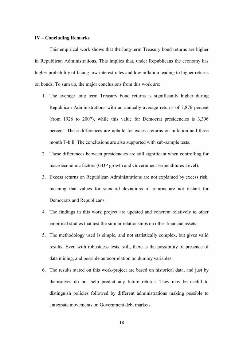
IV – Concluding Remarks

This empirical work shows that the long-term Treasury bond returns are higher

in Republican Administrations. This implies that, under Republicans the economy has

higher probability of facing low interest rates and low inflation leading to higher returns

on bonds. To sum up, the major conclusions from this work are:

1. The average long term Treasury bond returns is significantly higher during

Republican Administrations with an annually average returns of 7,876 percent

(from 1926 to 2007), while this value for Democrat presidencies is 3,396

percent. These differences are uphold for excess returns on inflation and three

month T-bill. The conclusions are also supported with sub-sample tests.

2. These differences between presidencies are still significant when controlling for

macroeconomic factors (GDP growth and Government Expenditures Level).

3. Excess returns on Republican Administrations are not explained by excess risk,

meaning that values for standard deviations of returns are not distant for

Democrats and Republicans.

4. The findings in this work project are updated and coherent relatively to other

empirical studies that test the similar relationships on other financial assets.

5. The methodology used is simple, and not statistically complex, but gives valid

results. Even with robustness tests, still, there is the possibility of presence of

data mining, and possible autocorrelation on dummy variables.

6. The results stated on this work-project are based on historical data, and just by

themselves do not help predict any future returns. They may be useful to

distinguish policies followed by different administrations making possible to

anticipate movements on Government debt markets.

19

19

V – References

Alexander, Carol. 2008. Practical Financial Econometrics. Chichester: Wiley.

Barsky, Robert.1989. “Why Don’t the Prices of Stocks and Bonds Move Together?”,

American Economic Review, Vol 79, no.5: 1132-1145.

Bordo, Michael, Joseph Haubrich. 2004. “The Yield Curve, Recessions, and the

Credibility of the Monetary Regime: Long-Run Evidence, 1975-1997”, Federal Reserve

Bank of Cleveland Working Paper Series, Working-Paper 04-02.

Campbell, John, Luis Viceira. 1999. “Who should buy long-term bonds?”, Harvard

Institute of Economic Research, Discussion Paper no.1985.

Caporal, Tony, Kevin Grier. 2005. “How Smart is my Dummy? Time Series Tests for

the Influence of Politics”, Political Analysis. vol13(1):77-94

Fama, Eugene, Kenneth French. 1989. “Business Conditions and the expected returns

on stocks and bonds”, Journal of Finance Economics 25: 23-49.

Fama, Eugene, Kenneth French. 1989. “Common factors affecting Bond and Stock

returns”

Goyal, Amit, Ivo Welch. 2007. “A Comprehensive Look at The Empirical Performance

of Equity Premium Prediction”

Grant, James, Emery Trahan. 2006. “Tactical asset allocation and presidential

elections”, Financial Services Review, 15: 151-165.

Hensel, Chris, William Ziemba. 1995. “United States Investment Returns during

Democratic and Republican Administrations”, 1928-1993”,Financial Analysts Journal,

Vol 51, no.2: 61-69

Ilmanen, Anti. 2003. “Stock-Bond Correlations”, Journal of Fixed Income, vol.13: 55-

66.

Jensen, Gerald, William Chittenden, Robert Johnson. 1999. “Presidential Politics,

Stocks,Bonds, Bills, and Inflation”, The Journal of Portfolio Management, Fall 1999

Parker, Elliot. 2006. “Does the Party in Power Matter for Economic Performance?”,

UNR Economics Working Paper Series – Working Paper 06-008.

Piazzesi, Monika. 2005. “Bond Yields and the Federal Reserve”, Journal of Political

Economy, vol.113: no. 2.

Piazzesi, Monika, Martin Schneider. 2008. “Inflation and the price of real assets”,

Federal Bank Reserve of Minneapolis, Staff Report no. 423.

Ramchander, Sanjay, Marc W. Simpson, James R. Webb. 2008. “Political Cycles

and REIT Returns”.

20

20

Santa Clara, Pedro, Rossen Valknov. 2003. “The Presidential Puzzle: Political Cycles

and the Stock Market”, Journal of Finance, 58: 1841-1871.

Verbeek, Marno. 2008. A Guide to Modern Econometrics. Chichester: John Willey &

Sons.

21

21

VI – Appendix

Table 1 – In this table are presented the statistical values for the quantitative variables used. The mean and standard

deviation are presented in annualized percentages, and in brackets are these quarterly values in percentage points. It

is also presented values for autocorrelation up to lag 4 (in quarters).

LTR LTR-TBL LTR-INF

Mean 5.704 [1.426] 1.92 [0.481] 4.949 [1.237]

Standard Deviation 8.584 [4.292] 8.692 [4.346] 8.695 [4.347]

Autocorrelation:

1 -0.052 -0.058 -0.044

2 0.029 0.020 0.033

3 0.107 0.104 0.108

4 0.013 0.005 0.015

GDP EXP

Mean 3.227 [0.807] 2.417 [0.604]

Standard Deviation 1.969 [0.985] 6.044 [3.022]

Autocorrelation:

1 0.329 0.484

2 0.181 0.374

3 -0.020 0.258

4 -0.113 0.124

Table 1 - Economic and Financial Variables

Table 2 – In this table are presented the list of Presidents, and the party in presidency that were considered in this

work. The dates represent signature days, so it is considered a cycle when the presidency officially starts and not on

election dates.

Republican/Democrat Mandate Start Mandate End

Calvin Coolidge R 02-08-1923 04-03-1929

Herbert Hoover R 04-03-1929 04-03-1933

F.D. Roosevelt D 04-03-1933 12-04-1945

Harry Truman D 12-04-1945 20-01-1953

Dwight Eisenhower R 20-01-1953 20-01-1961

John Kennedy D 20-01-1961 22-11-1963

Lyndon Johnson D 22-11-1963 20-01-1969

Richard Nixon R 20-01-1969 09-08-1974

Gerald Ford R 09-08-1974 20-01-1977

Jimmy Carter D 20-01-1977 20-01-1981

Ronald Reagan R 20-01-1981 20-01-1989

George Bush R 20-01-1989 20-01-1993

Bill Clinton D 20-01-1993 20-01-2001

George W. Bush R 20-01-2001 20-01-2009

Table 2 - Presidencial Cycles

22

22

Table 3 – Presidential cycles distribution by Republicans and Democrats (in quarters).

Presidency 1926:Q1 - 2007:Q4 1926:Q1 - 1961:Q4 1962:Q1 - 2007:Q4

Republicans 159 83 76

Democrats 169 61 108

Total 328 144 184

Table 3 - Political Variables

Chart 1 – Evolution of quarterly returns on long-term Treasury bonds. Sample: 1926:Q1 - 2007:Q4

Chart 2 – Evolution of Inflation and three month Treasury Bill. Annualized percentages .Sample: 1926:Q1 -

2007:Q4

Chart 1 - Evolution of LTR

-20.00%

-15.00%

-10.00%

-5.00%

0.00%

5.00%

10.00%

15.00%

20.00%

25.00%

30.00%

1925 1935 1945 1955 1965 1975 1985 1995 2005

Date

Quarterly Percentages

LTR

Chart - Evolution of TBL and INF

-6.00%

-4.00%

-2.00%

0.00%

2.00%

4.00%

6.00%

8.00%

10.00%

1925 1935 1945 1955 1965 1975 1985 1995 2005

Date

Annualized Percentages

INF

TBL

23

Table 4: This table presents the values for regressions (1), (2) and (3). DM and RP are the explanatory variables. The first horizontal line, for DM and RP set is the

coefficient value of the regression, the second line value is the standard deviation of the coefficient estimation, and the last line value in parenthesis is the p-value for

the null hypothesis that the coefficient is equal to zero. 2R is the adjusted R2 for the regressions. All regressions were calculated using OLS with Newey West

estimator corrections for autocorrelation and heteroskedasticity. Diff is represents the difference of the two coefficients (DM-RP). The values in this subset are result

for the Wald Tests on coefficient restrictions. The first value is the absolute difference, the below value is the standard deviation of the difference, the value in

parenthesis is the p-value for the F-test, and the p-value in brackets is the value for the Chi-Square test. Both tests are used to test the significance under the null

hypothesis, that the difference in the coefficients is equal to zero.

LTR LTR-TBL LTR-INF LTR LTR-TBL LTR-INF LTR LTR-TBL LTR-INF

DM 0.849 0.105 0.606 0.724 0.568 0.493 0.982 -0.387 0.726

0.303 0.315 0.262 0.221 0.226 0.227 0.582 0.602 0.504

(0.054) (0.738) (0.021) (0.001) (0.0131) (0.032) (0.093) (0.52) (0.151)

RP 1.969 0.834 1.83 0.921 0.316 1.014 2.576 1.134 2.304

0.357 0.357 0.372 0.351 0.360 0.375 0.518 0.524 0.519

(0.000) (0.02) (0.000) (0.009) (0.381) (0.007) (0.000) (0.031) (0.000)

N

0.014 0.003 0.016 0.001 0.002 0.004 0.016 0.014 0.015

Diff -1.120 -0.728 -1.225 -0.197 0.252 -0.521 -1.594 -1.521 -1.577

0.468 1.919 0.453 0.415 0.425 0.445 0.779 0.468 0.704

(0.017) (0.232) (0.007) (0.6358) (0.554) (0.243) (0.042) (0.468) (0.026)

[0.016] [0.233] [0.006] [0.6351] [0.553] [0.241] [0.040] [0.016] [0.025]

Table 4 - Results

328 144 184

1962:Q1 - 2007:Q41926:Q1 - 2007:Q4 1926:Q1 - 1961:Q4

2R

24

Table 5: This table presents the results from equations (4) ,(5) and (6). The methodology and results exhibit is similar to the regression in table 4.

LTR LTR-TBL LTR-INF LTR LTR-TBL LTR-INF

DM 0.382 -0.631 0.536 0.777 -0.387 0.546

0.923 0.967 0.563 0.632 0.663 0.931

(0.3684) (0.514) (0.341) (0.220) (0.559) (0.558)

RP 2.462 0.957 1.894 2.126 0.855 2.168

0.619 0.638 0.466 0.460 0.469 0.628

(0.000) (0.1359) (0.001) (0.000) (0.069) (0.000)

GDP 8.625 22.054 -0.587 -0.910 2.558 15.161

-22.147 57.442 27.51 29.526 31.266 54.722

(0.697) (0.701) (0.983) (0.9754) (0.934) (0.782)

EXP 12.240 7.103 -0.993 -0.787 0.314 8.794

54.188 22.262 6.89 7.571 7.463 22.194

(0.822) (0.750) (0.885) (0.917) (0.966) (0.692)

N

0.007 0.021 0.007 0.007 0.003 0.006

Diff -1.629 -1.588 -1.35 -1.348 -1.243 -1.622

0.853 0.875 0.639 0.668 0.0682 0.86

(0.057) (0.714) (0.034) (0.044) (0.069) (0.061)

[0.056] [0.069] [0.033] [0.43] [0.068] [0.059]

184 242

Table 5 - Results

1947:Q3 - 2007:Q41962:Q1 - 2007:Q4

2R

25

Table 6: Estimated values relative to equation (7). The dependent variables are VTL (total returns), VTL2 (excess returns on T-bill), and VTL3(excess returns on

inflation). All estimations were performed using OLS and Newey-West estimators to correct for autocorrelation and heteroskedasticity on residuals. 2R is the adjusted

R2 for the regressions. The first horizontal lines are the coefficient estimated for the average of squared deviations from the mean values. Diff is the difference between

the coefficients (DM-RP), The values in this subset are result for the Wald Tests on coefficient restrictions. The first value is the absolute difference, the below value is

the standard deviation of the difference; the value in parenthesis is the p-value for the F-test, and the value in brackets is the p-value for the Chi-Square test. Both tests

are used to test the significance under the null hypothesis, that the difference in the coefficients is equal to zero. On the last part of the table are presented the volatility

values based on the estimations. The first values are the squared roots of the coefficients yielding the quarterly volatility, while the last two lines represent the

annualised values for volatility (quarterly standard deviation annualization factor square-root of 4).

VTL VTL2 VTL3 VTL VTL2 VTL3 VTL VTL2 VTL3

DM 14.885 19.029 15.421 4.45 5.969 5.086 25.998 32.963 26.426

3.922 4.19 3.871 1.303 1.186 1.234 6.996 13.048 11.028

(0.000) (0.000) (0.000) (0.000) (0.000) (0.000) (0.000) (0.012) (0.017)

RP 21.744 22.67 22.174 7.819 10.514 7.953 29.812 29.713 30.414

3.540 2.950 3.570 1.499 2.236 1.878 5.934 4.715 6.056

(0.000) (0.000) (0.000) (0.000) (0.000) (0.000) (0.000) (0.000) (0.000)

N

0.001 0.001 0.001 0.012 0.017 0.007 0.000 0.000 0.000

Diff -6.858 -3.64 -6.753 -3.369 -4.544 -2.866 -3.813 3.222 -3.988

5.286 5.129 5.266 1.986 2.672 2.252 9.174 13754 12.602

(0.195) (0.478) (0.200) (0.092) (0.091) (0.205) (0.678) (0.815) (0.752)

[0.194] [0.477] [0.1998] [0.0899] [0.081] [0.203] [0.677] [0.814] [0.7517]

DM 3.858 4.362 3.927 2.110 2.443 2.255 5.099 5.741 5.141

RP 4.663 4.761 4.709 2.796 3.243 2.820 5.460 5.451 5.515

DM 7.716 8.724 7.854 4.219 4.886 4.510 10.198 11.483 10.281

RP 9.326 9.523 9.418 5.592 6.485 5.640 10.920 10.902 11.030

328 144 184

Volatility

Table 6 - Risk Analysis Results

1926:Q1 - 2007:Q4 1926:Q1 - 1961:Q4 1962:Q1 - 2007:Q4

2R