SEASONAL VARIATION IN TREASURY RETURNS∗

Mark J. KamstraSchulich School of Business

York UniversityEmail: mkamstra@yorku.ca

Tel: 416-736-2100 ext. 33302

Lisa A. KramerRotman School of Management

University of TorontoEmail: Lkramer@rotman.utoronto.ca

Tel: 416-978-2496

Maurice D. LeviSauder School of Business

University of British ColumbiaEmail: maurice.levi@sauder.ubc.ca

Tel: 604-822-8260

August 2011

JEL CLASSIFICATION: G11; G12; E43; E44KEYWORDS: Treasury bond returns; Treasury note returns;

market seasonality; time-varying risk aversion; SAD

ABSTRACT: We document a novel and striking annual cycle in the U.S. Treasury market, with avariation in monthly returns of over 80 basis points from peak to trough. We show that the seasonalTreasury return patterns we uncover are unlikely to arise due to macroeconomic seasonalities, seasonalvariation in risk, cross-hedging between equity and Treasury markets, conventional measures of investorsentiment, seasonalities in the Treasury market auction schedule, seasonalities in the Treasury debt supply,seasonalities in the FOMC cycle, or peculiarities of the sample period considered. The seasonal patternin Treasury returns is coincident with the incidence of seasonal depression observed clinically in NorthAmerican populations, which is noteworthy since depression has been shown to be associated with increasedfinancial risk aversion. The White (2000) reality test confirms that the correlation between returns and theclinical incidence of seasonal depression cannot be easily dismissed as the simple result of data snooping.

∗ We thank the editor and four anonymous referees for helpful suggestions. We have benefited from valuable conversations withHank Bessembinder, Michael Brennan, Hyung-Suk Choi, Ramon DeGennaro, Alex Edmans, Mark Fisher, Michael Fleming,Scott Frame, Ken Garbade, David Goldreich, Rob Heinkel, Shimon Kogan, Alan Kraus, and Monika Piazzesi. We thankseminar participants at the Federal Reserve Bank of Atlanta, the University of British Columbia, the University of Maryland,and the University of Utah, and conference participants at the Western Finance Association meetings, the European FinanceAssociation meetings, and the Northern Finance Association meetings. We gratefully acknowledge financial support of theSocial Sciences and Humanities Research Council of Canada and the Canadian Securities Institute Research Foundation. Anyremaining errors are our own.

SEASONAL VARIATION IN TREASURY RETURNSIn this paper we establish the presence of a striking anomalous seasonal pattern in U.S. Treasury

security returns. This seasonal pattern is strongly statistically and economically significant, with holders

of Treasuries earning a monthly return which peaks in autumn, declines monotonically through to spring,

and is on average 80 basis points higher in October than it is in April. Our focus is first to identify and

document the previously unknown seasonality in Treasury returns and to show that it is both economically

and statistically significant. Next we attempt to determine the exact source of the seasonal patterns in

Treasury returns, and while we find support for many of the existing hypotheses on bond return movements,

we demonstrate that none of these can easily account for the particular seasonal patterns we find. We

investigate the time-varying risk aversion hypothesis of Kamstra, Kramer, and Levi (2003) and find the

seasonal cycle in Treasury returns appears to be consistent with that hypothesis. Specifically, Treasury

returns are significantly positively correlated with the clinical incidence of seasonal depression in North

America. The underpinnings of this correlation may be a previously shown association between depression

and increased financial risk aversion, a possibility we explore using a variable based directly on the incidence

of seasonal depression in North America and using empirical asset pricing models.

A large literature has explored return patterns of risky assets and the factors that explain them (see

Cochrane (2005) for a comprehensive review of the asset pricing literature), however, much less attention

has been devoted to the seasonal movement in the riskfree rate of return. Several papers have shown

seasonalities in returns of various classes and maturities of bonds. These include Schneeweis and Woolridge

(1979) who demonstrate the presence of autocorrelation in bond index returns; Jordan and Jordan (1991)

who find no evidence of a day-of-the-week effect in corporate bonds over the past few decades but do find

evidence of a January seasonal, a week-of-the-month effect, and a turn-of-the-year effect; and Chang and

Huang (1990) and Wilson and Jones (1990) who demonstrate the presence of a January seasonal in various

U.S. corporate bond returns. Other papers have attempted to explain time-varying bond returns based

on time-varying risk. For example, Boudoukh (1993) considers macroeconomic factors like consumption

growth and inflation. Connolly, Stivers, and Sun (2005) find that Treasury and stock markets can move in

opposite directions for short periods, perhaps due to cross-market hedging. De Bondt and Bange (1992)

and Brandt and Wang (2003) suggest that predictable, time-varying term premia on government bonds

could arise due to unexpected inflation. Still other studies have explored the possibility of time-varying

risk aversion having an influence on government bond returns. For instance, Ilmanen (1995) examines

long-term government bond returns in six countries and finds evidence of risk premia that depend on

aggregate relative wealth measures. There is a closely related literature on bond yields that demonstrates

time-varying risk premiums on nominal bonds. See, for instance, Ang and Piazzesi (2003) and Cochrane

and Piazzesi (2005) for some recent evidence, and the classic work of Fama and Bliss (1987) and Campbell

and Shiller (1991). Work on yields strongly supports bond return predictability based on yield spreads

and macroeconomic factors. Collectively, these studies suggest possible sources for seasonality in Treasury

returns, and each is explored below. There are also behavioral explanations that potentially underlie the

1

seasonality we demonstrate, for instance investor sentiment.1 Baker and Wurgler (2006) find investor

sentiment can impact security returns, and so we utilize their measure, as well as the Michigan consumer

sentiment index, to explore whether sentiment helps explain the seasonal Treasury return pattern we

illustrate.

Our findings contribute to the body of evidence that even in markets dominated by professional market

participants, returns can be influenced by behavioral considerations. For example, Goldreich (2005) shows

that Treasury market dealers submit bids in price space that are dominated in yield space, suggesting

bounded rationality among these professionals. Further, Cici (2005) finds that the trades and performance

of mutual fund managers exhibit some evidence of the disposition effect. Our paper also joins the growing

body of literature that explores the possible influence of affect (emotions) on financial markets. See Kamstra

et al. (2001, 2003), Statman, Fisher, and Anginer (2008), Bracha and Brown (2008), and Kaplanski and

Levy (2008) for instance.

The remainder of the paper is organized as follows. In Section 1 we present evidence of a statistically

significant and economically large seasonal cycle in Treasury returns. In Section 2, we consider the pos-

sibility that the seasonal pattern arises due to time-varying risk aversion linked to seasonal depression,

and find results that are strongly suggestive of this possibility. In Sections 3 and 4 we consider a broad

range of alternative possible explanations for the seasonal pattern in Treasury returns, including macroeco-

nomic shocks, cross-hedging (whereby periods of stock market uncertainty may induce effects in Treasury

returns), investor sentiment, the Fama-French and momentum risk factors, and several factors related to

activities of the U.S. Treasury and Federal Reserve. Possible Treasury and Federal Reserve influences that

we consider include the management of the supply of Treasury debt, the Federal Reserve Board’s annual

cycle of rate-setting meetings, and a significant change to the Treasury auction announcement policy that

was introduced in the late 1970s to facilitate liquidity in the Treasury market. We find that none of these

alternatives is capable of fully explaining the seasonal pattern in Treasury returns. Further, we find the

time-varying price of risk is correlated with seasonal depression in a conditional CAPM setting, consistent

with the hypothesis that the seasonal return pattern arises due to time-varying risk aversion. In Section 5,

using the White (2000) reality test, we show that the relation between seasonal depression and Treasury

returns is unlikely to be a result of data mining. In Section 6 we report on a variety of sub-sample analyses

to investigate the stability of this seasonality. We find that evidence of the seasonality did not appear until

after Treasury introduced auctions to the sale of notes and bonds in the 1970s; before this market-driven

pricing setting mechanism was in place we see little seasonality in note and bond returns. However, after

auctions were introduced and a regular, predictable schedule of Treasury issuance was in place in the early

1980s, seasonality in Treasury returns became a stable feature of the data. We conclude with Section 7.

1Note that “sentiment” typically refers to investor mistakes. For example, Shefrin (2008, p. 213) observes “in finance,sentiment is synonymous with error ... errors of individual investors, particularly representativeness and overconfidence,combine to produce market sentiment.” Sentiment could encompass the time-varying risk aversion we investigate, but forsimplicity we refer to sentiment and time-varying risk aversion as distinct concepts.

2

1 TREASURY RETURNS

In this section we document seasonal patterns in Treasury returns, based on both nominal returns and

returns in excess of the 30-day T-bill rate (which we generically refer to as “excess” returns). We consider

monthly returns to holding the medium-to-long end of Treasury market securities, specifically 20-year,

10-year, 7-year, and 5-year Treasury bond and note returns, where the returns include interest and capital

gains/losses. We consider data from 1952 onward, consistent with Campbell’s (1990) observation that

interest rates were almost constant in the United States until 1951, after which an accord between the

Federal Reserve Board and the U.S. Treasury permitted interest rates to respond more freely to market

forces. We limit our primary focus to the medium-to-long end because rate movements in the short end

do not respond freely to market forces, even following the accord between the U.S. Treasury and the

Federal Reserve Board. Gibson (1970), for instance, notes in reference to the short end that an “aim of

the Federal Reserve System is to accommodate seasonal swings in the financial needs of trade, and the

System tries to do this by removing seasonal fluctuations from interest rates (p.442).” In Appendix A we

do, however, provide results for the short end of the Treasury market and we discuss related institutional

detail. These results show evidence of seasonality in the short end, though weaker than found in the

longer-term Treasuries.2

The Treasury index return data are from the Center for Research on Security Prices (CRSP) U.S.

Treasury and Inflation Series. We require an equity return series for reference and for the calculation of

some statistics; we employ the CRSP U.S. stock index, value-weighted, including distributions. In the

top portion of Table 1 we present summary statistics on the monthly Treasury index return data, both

nominal and in excess of the 30-day T-bill rate, and in the last panel of Table 1, labeled “Other Data

Used As Instruments,” we provide summary statistics on the monthly stock index returns. Table 1 also

contains the results of seasonality tests. The seasonality tests we consider are motivated with reference

to Kamstra et al. (2003), following from their observation that “on balance the seasonally asymmetric

effects of SAD [a form of seasonal depression] are shifting [stock] returns from the fall to the winter (p.

336).” Our hypothesis is that time-varying risk aversion due to seasonal depression also drives seasonal

patterns in Treasury returns, shifting them from the winter to the fall.3 We elaborate on the specifics

of this hypothesis in the next section, but first we document the annual seasonality that we find in the

Treasury return data.

The average of each of the monthly nominal (excess) Treasury index return series is roughly 50 (10)

basis points. The standard deviations of the Treasury index returns are well below that of the equity index

over the same period, increasing monotonically with maturity, and the minimum and maximum observed

for each Treasury series generally span a smaller range as maturity shortens. The stock index has a mean

return close to one percent per month, ranging from a minimum below -22 percent to a maximum of

2Gibson (1970) also notes weak seasonal patterns in 90-day T-bill rates.3Kamstra, Kramer, Levi, and Wang (2011) explore an asset pricing model with a representative agent who experiences

seasonally varying risk preferences. They find plausible values of risk-preference parameters are capable of generating theempirically observed seasonal patterns in equity and Treasury returns.

3

almost 17 percent, and a standard deviation exceeding 5 versus 2.64 for the 20-year U.S. Treasury index.

Exposure to market risk is a traditional measure of systemic risk, thus we also report the capital asset

pricing model (CAPM) beta for each of the individual Treasury series. Beta is measured by regressing the

Treasury excess returns on the equity index excess returns. The beta of all the Treasury classes is virtually

zero.4 All the series are leptokurtotic and skewed toward positive returns. We return to discussing the

remaining columns and panels of Table 1 later.

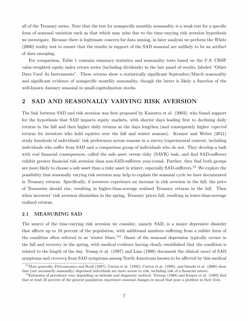
Figure 1 contains plots of the monthly average Treasury excess return series. Results are qualitatively

identical for nominal returns. Panel A depicts monthly Treasury excess returns averaged across the 20-

, 10-, 7-, and 5-year maturities, represented with a heavy solid line. Dotted lines depict a 90 percent

confidence interval around the monthly means.5,6,7 The thin solid line with circles represents the average

annual return, and an X appears over the circle in months where the average return falls outside of the

confidence interval. Monthly average Treasury excess returns are high and above the annual average (of

approximately .13 percent) through the fall months and are below average in the winter months. In April,

the monthly average excess return reaches its lowest point of the year. The decline in returns is monotonic

from the annual peak in October to the annual trough in April. Further, the magnitude of the decline in

average monthly returns from October through to April is striking: the difference is about 80 basis points.

The decline from October to April is also statistically significant, and five months of the year (September,

October, November, March, and April) are significantly different from the annual mean. Panel B contains

plots of each of the four individual average monthly Treasury excess return series, which all show very

similar seasonal variation.

Formal tests also support the notion that Treasury returns are in effect shifted between the fall and

winter seasons. We consider three tests. First, we use a dummy variable equal to one in the fall (October,

November, and December), equal to minus one in the winter (January, February, and March), and equal

to zero otherwise (Dt,fall/winter). Second, we employ a dummy variable equal to one in September, equal

to minus one in March, and equal to zero otherwise (Dt,Sept/Mar). Third, we explore use of a dummy

4It is a commonly held belief that short- and long-term Treasury securities represent a safe haven from risk. For example,during the 2008/2009 financial crisis, and even in the most recent financial crisis in August 2011, all Treasury maturities werein high demand. Press coverage on this matter includes Wall Street Journal articles by Lauricella et al. (2011) and Zeng(2011).

5There are several approaches one could adopt to calculate the confidence interval around the mean monthly returns. Thesimplest is to use the standard deviation of the monthly mean returns directly. However, this would ignore information aboutthe cross-sectional variability of returns across the four Treasury series. Instead, we form a system of equations with thefour series and estimate a fixed-effects model with twelve dummy variables (one for each month). Consistent with the typicalimplementation of a fixed effects model, we allow each series to have a different mean, while estimating one set of parametervalues for the variables each series has in common, in this case the monthly dummy variables. From this regression we obtainstandard errors on the monthly dummies to form the confidence intervals around the monthly mean returns.

6We use Hansen’s (1982) generalized method of moments (GMM) and Newey and West (1987) heteroskedasticity andautocorrelation consistent standard errors, and following Newey and West (1994) we use the Bartlett kernel and an automaticbandwidth parameter (autocovariance lags) equal to the integer value of 4(T/100)2/9. The moment conditions we use includeorthogonality between a small set of instruments and the errors. For instruments we use the constant, a lag of the CRSPvalue-weighted return (entire U.S. market return, including dividends), the contemporaneous 30-day T-bill rate as suggestedby Ferson and Foerster (1994), and the 12 monthly dummy variables. The confidence intervals are similar if we use fullinformation maximum likelihood and MacKinnon and White (1985) bootstrap heteroskedasticity-consistent standard errors.For a detailed discussion on the use of GMM, see Cochrane (2001), Chapters 10 and 11.

7Occasionally returns and standard errors change by offsetting amounts making the confidence bands appear nearly flat.

4

Average Treasury Excess Returns Individual Treasury Excess Returns

Figure 1: This figure contains plots of monthly Treasury returns in excess of the 30-day Treasury bill rate, obtained fromCRSP. Panel A depicts monthly Treasury returns averaged across the 20-, 10-, 7-, and 5-year maturities. A heavy solid linerepresents the monthly mean residuals and dashed lines represent a 90 percent confidence interval around the monthly means.The average annual return appears as a solid line with circles (and an X in cases where the average return falls outside theconfidence interval). In Panel B we plot each Treasury return series individually. The 5-year, 7-year, 10-year, and 20-yearseries are represented by lines with solid circles, asterisks, hollow squares, and hollow circles respectively. The data spanJanuary 1952 through December 2007.

variable equal to one in October, equal to minus one in April, and equal to zero otherwise (Dt,Oct/Apr).

The October/April and September/March dummy variable specifications come closest to matching the

timing of initial onset and initial recovery from SAD documented in clinical studies of individuals who

suffer from the condition (we elaborate on these studies below), and the fall/winter dummy variable should

pick up the average impact across the the full fall and winter seasons. Our null hypothesis is that there is

no seasonal difference in returns, i.e., that the coefficient on a given dummy variable is zero, against the

alternative of returns being shifted from winter into fall. The SAD hypothesis implies that these dummy

variables should have positive coefficients when applied to Treasury returns.

For instance, to test whether a Treasury return series has the same mean value in the fall and winter

versus the alternative that the fall and winter means deviate from the annual average by an equal and

opposite amount, we estimate the following model:

ri,t = αi + βi,fall/winterDt,fall/winter + εi,t.

The dependent variable is the Treasury return series, where i indexes 5-, 7-, 10-, or 20-year maturity. We

estimate alternate versions of this model to produce the various seasonality tests, replacing Dt,fall/winter

with either Dt,Sept/Mar or Dt,Oct/Apr. A given seasonality test is a two-sided t-test on the dummy variable

coefficient to differ from zero. We also perform a test for seasonal variation of nonspecific form, involving

a regression of the return series on a constant and monthly dummy variables, excluding January. We

test whether the monthly dummy variables jointly differ from zero, an eleven degree of freedom χ2 test.

Each seasonality test is performed by estimating the model using Hansen’s (1982) generalized method

5

of moments (GMM);8,9 tests are performed using Newey and West (1987, 1994) heteroskedasticity and

autocorrelation consistent (HAC) standard errors. See footnote 6 for details. The HAC standard errors

control for well-known heteroskedasticity and autocorrelation effects in returns. Note that we employ

GMM and Newey and West (1987, 1994) standard errors for all estimations reported in this paper. Two

sets of p-values are produced for each seasonality test, one based on asymptotic standard errors,10 and one

based on bootstrapping the distribution of the test statistic.11,12 The last four columns of Table 1 contain

the results of seasonality tests on the Treasury return series. We report tests based on nominal Treasury

returns, Treasury returns in excess of the 30-day Treasury rate, an equal-weighted average of the four

nominal Treasury return series, and an equal-weighted average of the four excess Treasury return series.

In each cell, we provide the asymptotic p-value and the bootstrapped p-value in square brackets below.

Cases significant at the 10 percent level or better are indicated in bold. We consider first asymptotic p-

values for the three tests for seasonality of a specific form. All of the Treasury return series exhibit strong

seasonality, with each exhibiting p-values below .1 percent for the October/April test, all but the 10-year

returns exhibiting p-values below 10 percent for the fall/winter test, and all but the 10- and 20-year returns

exhibiting p-values below 10 percent for the September/March test. Considering the nominal and excess

average returns across the series, we reject the null at the 10 percent level or better for all three sets of

seasonality tests of specific form. Analysis based on the bootstrapped distributions of these test statistics

verifies the robustness of the finding of seasonality. The test for nonspecific monthly seasonality, based on

regressing returns on a constant and a dummy variable for each month except January, is insignificant for

8The moment conditions we use include orthogonality between a small set of instruments and the errors. For instrumentswe use the constant, a lag of the CRSP value-weighted return (entire U.S. market return, including dividends), the contem-poraneous 30-day T-bill rate as suggested by Ferson and Foerster (1994), and the dummy variables used for the regressionslightly modified as follows: For the fall versus winter seasonality test, dummies for the fourth and first quarters are includedin the instrument list, for the September versus March seasonality test, dummies for September and March are included, andfor the October versus April seasonality test, dummies for October and April are included.

9Hansen (1982), Staiger and Stock (1997), and Stock and Wright (2000) detail conditions sufficient for consistency andasymptotically normality of GMM estimators.

10Results are very similar if we use full information maximum likelihood estimation and MacKinnon and White (1985)bootstrap heteroskedasticity-consistent standard errors, and/or if we include a sufficient number of lags of the dependentvariable to directly control for return autocorrelation.

11Ferson and Foerster (1994) note that in cases where there are too many over-identifying restrictions relative to the samplesize, the asymptotic distribution of test statistics can be a poor approximation of the finite-sample test distribution.

12 We employ block bootstrap resampling to allow for data dependence, as detailed by Politis and Romano (1994) andemployed by White (2000). Politis and Romano (1994) show that this technique produces valid bootstrap approximationsfor means of alpha-mixing processes, so long as the block length increases with sample size. Results of Goncalves and White(2002, 2005) establish the consistency of the bootstrap variance estimator of Politis and Romano (1994) for the sample meanin the presence of heteroskedasticity and dependence of unknown form. Politis and Romano (1994) use blocks of data ofrandom length, distributed according to the geometric distribution with mean block length b. The parameter b is chosen sothat block length is data-dependent, with Politis and Romano (1994) recommending a scaling proportional to N1/3, whereN=sample size. The setting b = N1/3 would lead to a mean block length of approximately 9 observations in our sample,which is a fairly long block length for monthly return data. White (2000) remarks that a mean block length of 10 for dailydata is appropriate given the weak autocorrelation of returns. This would translate to the minimum mean block length of 2for our monthly data. We set the block length to 5 but find our results are virtually identical for block lengths between 2 and10. We use 1,000 resamples, which we find produces stable results. White (2000) suggests 500 or 1,000 resamples and uses 500in his empirical application on S&P 500 stock returns. Although the tests reported in Table 1 are all one series at a time, weperform much of the subsequent analysis on all four Treasury series with system-of-equation estimation. Rilstone and Veall(1996) show substantially better inference can result using the bootstrap in a system-of-equations estimation context. Palmet al. (2008) show asymptotic validity of block bootstrap tests in the context of panel data with cross-sectional dependence.

6

all of the Treasury series. Note that the test for nonspecific monthly seasonality is a weak test for a specific

form of seasonal variation such as that which may arise due to the time-varying risk aversion hypothesis

we investigate. Because there is legitimate concern for data mining, in later analysis we perform the White

(2000) reality test to ensure that the results in support of the SAD seasonal are unlikely to be an artifact

of data snooping.

For comparison, Table 1 contains summary statistics and seasonality tests based on the U.S. CRSP

value-weighted equity index return series (including dividends) in the last panel of results, labeled “Other

Data Used As Instruments”. These returns show a statistically significant September/March seasonality

and significant evidence of nonspecific monthly seasonality, though the latter is likely a function of the

well-known January seasonal in small-capitalization stocks.

2 SAD AND SEASONALLY VARYING RISK AVERSION

The link between SAD and risk aversion was first proposed by Kamstra et al. (2003), who found support

for the hypothesis that SAD impacts equity markets, with shorter days leading first to declining daily

returns in the fall and then higher daily returns as the days lengthen (and consequently higher expected

returns for investors who hold equities over the fall and winter seasons). Kramer and Weber (2011)

study hundreds of individuals’ risk preferences across seasons in a survey/experimental context, including

individuals who suffer from SAD and a comparison group of individuals who do not. They develop a task

with real financial consequences, called the safe asset versus risky (SAVR) task, and find SAD-sufferers

exhibit greater financial risk aversion than non-SAD-sufferers year-round. Further, they find both groups

are more likely to choose a safe asset than a risky asset in winter, especially SAD-sufferers.13 We explore the

possibility that seasonally varying risk aversion may help to explain the seasonal cycle we have documented

in Treasury returns. Specifically, if investors experience an increase in risk aversion in the fall, the price

of Treasuries should rise, resulting in higher-than-average realized Treasury returns in the fall. Then

when investors’ risk aversion diminishes in the spring, Treasury prices fall, resulting in lower-than-average

realized returns.

2.1 MEASURING SAD

The source of the time-varying risk aversion we consider, namely SAD, is a major depressive disorder

that affects up to 10 percent of the population, with additional numbers suffering from a milder form of

the condition often referred to as ‘winter blues.’14 Onset of the seasonal depression typically occurs in

the fall and recovery in the spring, with medical evidence having clearly established that the condition is

related to the length of the day. Young et al. (1997) and Lam (1998) document the clinical onset of SAD

symptoms and recovery from SAD symptoms among North Americans known to be affected by this medical

13More generally, Pietromonaco and Rook (1987), Carton et al. (1992), Carton et al. (1995), and Smoski et al. (2008) showthat (not necessarily seasonally) depressed individuals are more averse to risk, including risk of a financial nature.

14Estimates of prevalence vary depending on latitude and diagnostic method. Terman (1988) and Kasper et al. (1989) findthat at least 25 percent of the general population experience seasonal changes in mood that pose a problem in their lives.

7

condition. These data indicate that most SAD-sufferers begin experiencing their symptoms in early-to-mid

fall and fully recover by early spring, though exact timing varies by individual.15,16 (Note that Harmatz

et al. (2000) provide evidence that even individuals who do not suffer from the medical condition SAD

experience significant seasonal changes in depression, with depression peaking in winter.) With a portion

of the population suffering from depression and heightened risk aversion during the fall and winter seasons,

Kamstra et al. (2003) relate equity returns to the number of hours of daylight utilizing a length of night

variable and a fall dummy variable. (See Kamstra et al. (2003) for further details on their rationale for

this two-variable specification.) They demonstrate that this specification captures a remarkable cycle in

equity returns.

The specification that Kamstra et al. (2003) employ is a proxy for SAD onset and recovery. We consider

in place of their variables an alternative measure linked directly to the clinical incidence of SAD, constructed

using the Lam (1998) data on SAD patients’ timing of onset and recovery.17 Details on the construction of

this measure are as follows. First, we form a SAD ‘incidence’ variable which reflects the monthly proportion

of SAD-sufferers who are actively experiencing SAD symptoms in a given month. The incidence variable

is calculated by cumulating, monthly, the proportion of subjects who have experienced the onset of their

SAD symptoms (cumulated starting in late summer, when a small proportion of subjects are first diagnosed

with onset) and then deducting the cumulative proportion of people who have experienced full recovery

from SAD. The resulting monthly incidence variable takes on values between zero percent, in summer, and

close to 100 percent, in winter. This measure of SAD incidence is based on estimates of onset and recovery

in the broader population of all North Americans who suffer from SAD, hence incidence is measured with

error. To avoid an error-in-variables bias (see Levi (1973)), we construct an instrumented version of the

incidence variable.18 Finally, the monthly change in this instrumented incidence variable yields the SAD

onset/recovery used in our tests, which we denote ORt (short for onset/recovery, with the hat indicating

15Young et al. (1997) study 190 Chicago residents with SAD and find that 74 percent of them are first diagnosed with SADbetween mid-September and early November. Lam (1998) studies 454 SAD patients in Vancouver and also finds that the peaktiming of onset is in early fall. Lam further establishes that the timing of clinical remission from SAD peaks in April, closelyfollowed by March. Onset and recovery are typically separated by several months.

16September and October are the months during which the highest proportion of individuals experience the onset of SAD.If investors begin rearranging their portfolios when they first become risk averse, then September and October should bethe approximate time of year when we observe the largest positive impact on Treasury returns due to SAD. Although someindividuals begin recovering from SAD in January, the peak time for recovery is March/April. Thus we should see SADimpacting returns as early as January, but the peak effects should occur roughly in March/April. In short, security returns,which are an income flow, should respond to the flow of SAD-affected investors, not the stock of actively suffering SAD-affectedinvestors.

17There exist other clinical studies that document the timing of SAD symptoms, including Young et al. (1997). We baseour measure on data from the Lam (1998) study because, unlike other clinical studies, his details the timing of both onset andrecovery. Our measure and findings are qualitatively identical if we combine data from the Lam and Young et al. studies.

18To produce the instrumented version of incidence, first we smoothly interpolate the monthly incidence of SAD to dailyfrequency using a spline function. We need to produce an instrumented value of incidence that is strictly positive but no morethan 100 percent, so we run a logistic regression of the daily incidence on our chosen instrument, the length of day. (Thenonlinear model is 1/(1 + eα+βdayt), where dayt is the length of day t in hours in New York and t ranges from 1 to 365. Theβ coefficient estimate is 1.18 with a standard error of .021, the intercept estimate is -13.98 with a standard error of .246, andthe regression R2 is 94.9 percent.) The fitted value from this regression is the instrumented measure of incidence. Employingadditional instruments, such as change in the length of the day, makes no substantial difference to the fit of the regression orthe subsequent results using this fitted value.

8

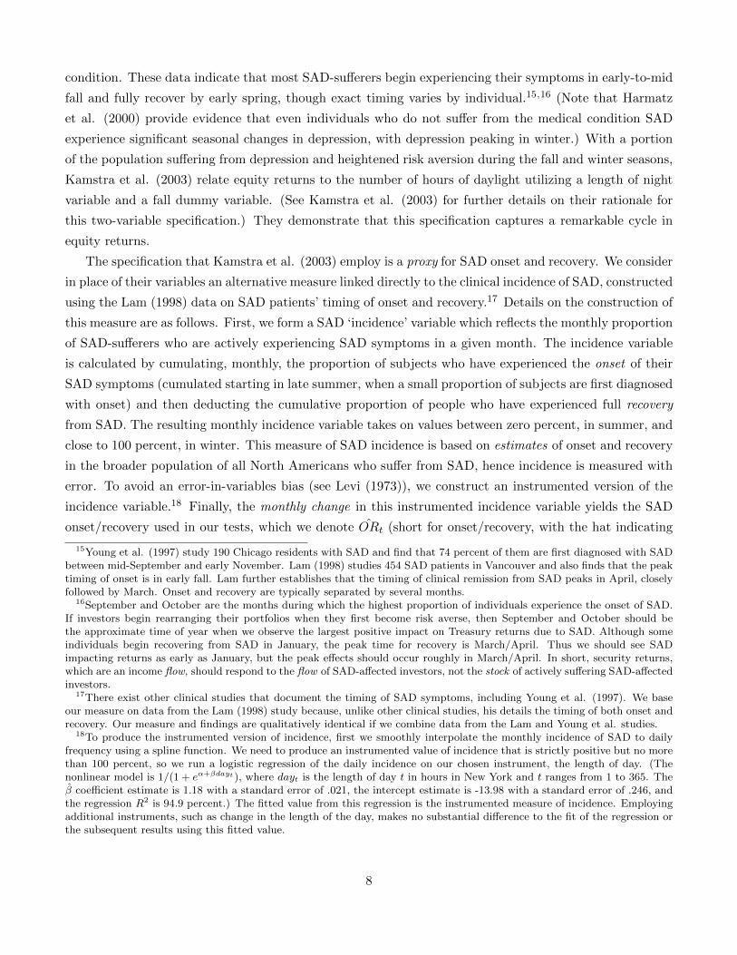
Figure 2: SAD Onset/Recovery and Change in Length of Night. The onset/recovery variable reflects the change in theproportion of SAD-affected individuals actively suffering from SAD. The monthly series, calibrated to the 15th day of each month, isbased on the clinical incidence of SAD symptoms among patients who suffer from the condition. The thick plain line plots the SADonset/recovery variable (ORt), the thin plain line plots observed onset/recovery, and the line with circles is the change in the length ofnight, normalized by dividing by 12 (the average annual length of night).

the variable is the fitted value from a regression). More specifically, the monthly variable ORt is calculated

as the value of the daily instrumented incidence value on the 15th day of a given month minus the value

of the daily instrumented incidence value on the 15th day of the previous month.19,20

ORt reflects the change in the proportion of SAD-affected individuals actively suffering from SAD. The

monthly values of ORt are plotted as a thick plain line in Figure 2, starting with September and ending

with August, together with the corresponding values of ORt (thin plain line) and the change in the length

of night divided by 12 (thin line with circles). Notice that all measures are positive in summer and fall and

negative in winter and spring. The values peak near fall equinox and reach a trough near spring equinox.

A noteworthy feature of the onset/recovery variable is that it is based directly on the clinical incidence

of SAD in individuals, unlike Kamstra et al.’s (2003) variables. Also, it spans the entire year, whereas

Kamstra et al.’s (2003) length of night and fall dummy variables take on non-zero values during the fall

and winter months only (and therefore cannot account for the portion of SAD-sufferers who experience

symptoms earlier than fall or later than winter).

2.2 DOES SAD HELP EXPLAIN THE TREASURY RETURN ANNUAL CYCLE?

We turn now to testing whether the onset/recovery variable helps explain the seasonal patterns in Treasury

returns evident in Table 1 and Figure 1. Excess returns are required for some of the alternative models we

consider, thus we focus on excess returns in our regression analysis. Results are virtually identical when

using nominal returns. We regress excess Treasury returns on ORt:

19The values of ORt by month, rounded to the nearest integer and starting in July, are: 3, 15, 38, 30, 8, 1, -5, -21, -42, -21,-5, 0. These values represent the instrumented change in incidence of symptoms. The correlation of the instrumented fittedvalue with the realized onset/recovery is .96 and the correlation of the fitted value with the change in length of night is .91.

20We find qualitatively identical results when we perform our analysis replacing ORt with either ORt or the change in thelength of night. See Appendix B.

9

(1) ri,t = µi + µi,ORORt + εi,t.

Table 3 contains the system-of-equations estimation results using Hansen’s (1982) GMM and Newey and

West (1987, 1994) standard errors, accounting for cross-equation covariance between the four return series,

and heteroskedasticity and autocorrelation in returns.21,22 For additional technical estimation details, see

the notes to Table 3. In Panel A we see that the OR coefficients on all four Treasury series are positive

and significant. The onset/recovery variable itself is positive in the fall and negative in the winter, thus the

positive coefficients imply above-average Treasury returns in the fall and below-average Treasury returns

in the winter.

Panel B of Table 3 contains the magnitudes of seasonal variations in returns, by series, calculated based

on both realized and fitted returns. We consider seasonal variation in returns from fall to winter, September

to March, and October to April. In each case the variations for the “realized” series are positive, ranging

in magnitude from a low around 30 basis points to a high over 90 basis points. The variations for the

“fitted” series reveal that the model is accurately capturing seasonal variability in Treasury returns, both

in terms of sign (positive) and on the basis of rough magnitudes.

The first two lines of Panel C contain joint tests on the onset/recovery coefficients across the four

Treasury series, the first testing whether the estimates are jointly zero and the second testing whether

they are jointly equal (but not necessarily zero). We present asymptotic and bootstrapped p-values. This

bootstrap technique employs resampling of blocks of data, preserving the cross-sectional correlation of the

Treasury series and producing resampled statistics that are also robust to data dependence. See footnote

12 for details on our bootstrap technique. We reject the null that the onset/recovery coefficients are jointly

zero, with a p-value below 3 percent. Overall, the results are consistent with investors shunning risk in

21The instruments we use in all of our regressions to form the GMM moment conditions, unless noted otherwise, are aconstant, the explanatory variables (in Equation (1) this is ORt), 30-day T-bill returns, and the lagged CRSP value-weightedequity index returns including dividends. See footnote 6 for further estimation details.

22Throughout the paper, regression results are very similar if we use full information maximum likelihood (FIML) orseemingly unrelated regression rather than GMM, and/or if we include a sufficient number of lags of the dependent variable todirectly control for return autocorrelation, and/or if we introduce small changes in the number of instruments used to identifymodel parameters and window width smoothing parameters employed in GMM estimation. (See Appendix C for resultsbased on FIML.) In general, the more instruments used to identify model parameters, the more significant are the parameterestimates, consistent with the intuition that the more over-identifying information used, the better we are able to estimateparameters of the system. The small-sample properties of our tests degrade with excessive numbers of moment conditions,however. Ferson and Foerster (1994) consider the use of GMM and HAC standard errors in the context of a system-equationestimation with monthly U.S. Treasury and stock returns. They perform Monte Carlo experiments to evaluate the small-sampleperformance of GMM and HAC standard errors with system-equation estimation and testing in the presence of autocorrelationand ARCH. Their case of sample size N=720, with 5 equations and a small instrument set of 3 variables, is closest to most ofour model estimations, in particular our onset/recovery model. The GMM approach shows poor performance when very smalldata sets are used, 60 observations, and even with moderately sized datasets with many instruments (numbering 8 relative to1 or 3 parameters per equation). But with a large number of observations, such as we employ, even use of a large number ofinstruments does not compromise performance markedly. We work with over-identified models, though none are as heavilyover-identified as the extreme case Ferson and Foerster explore. Finally, their main experiments do not incorporate conditionalheteroskedasticity, but their main results are robust to the impact of conditional heteroskedasticty, as they describe in Section5.4 of their paper. Ferson and Harvey (1992) provide a review of the literature on simulation studies of GMM estimation insmall samples that also strongly supports the use of GMM methods in samples as large as ours, spanning about 50 years ofmonthly data.

10

the fall, resulting in higher Treasury prices (and higher realized Treasury returns) in the fall than would

otherwise be the case. Similarly, the results are consistent with investors resuming their previous level of

risk aversion as daylight becomes more plentiful through the winter season, resulting in lower Treasury

prices (and lower realized Treasury returns) than would otherwise be the case.

The remaining lines in Panel C contain p-values associated with the tests for residual seasonality across

all of the return series. These tests are analogous to the seasonality tests performed in Section 1 on

the raw and excess Treasury returns, one series at-a-time, but now we explore whether there exists joint

seasonality across the four series after having controlled for onset/recovery. For instance, the test for

nonspecific monthly seasonal variation involves a regression of the return series on a constant, OR, and 11

monthly dummy variables, restricting coefficients on the dummy variables to have the same value across

series. That is

ri,t = αi + µi,ORORt +

12∑j=2

βjDj,t + εi,t,

where Dj,t is a dummy variable equal to 1 if the month of the year for observation t equals j (with February

designated month 2, March month 3, and so on). We test whether the monthly dummy coefficients each

equal zero, an eleven degree of freedom χ2 test. To test whether a Treasury return series, controlling for

onset/recovery, has the same mean value in the fall and winter versus the alternative that the fall and

winter means deviate from the annual average by an equal and opposite amount, we estimate the following

model:

ri,t = αi + µi,ORORt + βfall/winterDt,fall/winter + εi,t.

Note again that the coefficient on the seasonality test variable, βfall/winter, is restricted to have the same

value across series. We estimate alternate versions of this model to produce the alternate seasonality tests,

replacing Dt,fall/winter with either Dt,Sept/Mar or Dt,Oct/Apr. A given test for seasonality is a two-sided

t-test on the dummy variable coefficients to each equal zero.23

We see in Panel C of Table 3 that all four test statistics (associated with the test for nonspecific monthly

seasonality and the three tests for SAD-related seasonality) are insignificant. That is, there is no significant

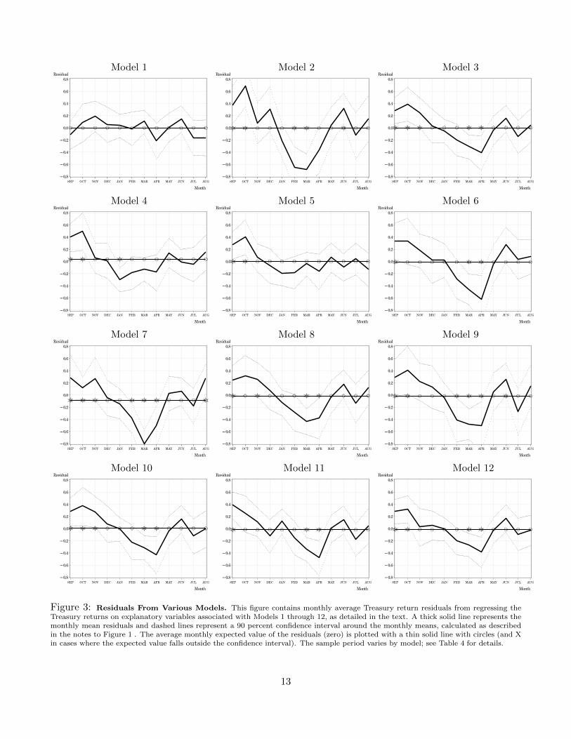
evidence of seasonal variation in the returns if we control for onset/recovery. In Figure 3, the panel labeled

“Model 1” contains a plot of the monthly mean Treasury return residuals from the regressions; we consider

Models 2-12 later. Observe that the seasonal pattern in the residual series is largely purged. All of the

monthly mean bond residuals lie within the confidence interval around the expected value of zero. As we

show in the next section, the magnitude of the deviations around zero is smaller than that achieved by

other models and the confidence intervals are no wider than produced by other models. That is, the lack of

statistically significant seasonality in the monthly residuals is not an artifact of a relatively noisy regression

error.

In Panel D of Table 3 we provide estimation details including sample period, number of observations

and model parameters, number of moment conditions, a GMM test of overidentifying restrictions, and

23In unreported analysis, we found that the restriction of constant coefficients on the seasonality variables Dt,fall/winter,Dt,Sept/Mar, and Dt,Oct/Apr, relative to the unrestricted case with the coefficients allowed to vary across Treasury series i, hadlittle qualitative effect on test results.

11

two information criteria (labeled MMSC-BIC and MMSC-HQIC) specifically designed by Andrews and Lu

(2001) for application to GMM estimation in a dynamic panel setting. Lower values of the criteria identify

better model performance. For each information criterion we present two values. One is for the model that

includes onset/recovery and the other is for a model that includes only a constant. On the basis of both

criteria, we see that the onset/recovery model performs better than a constant return model. The test of

overidentifying restrictions, χ2 with 8 degrees of freedom, does not reject the null of no misspecification.

3 ALTERNATIVE MODELS

In this section we consider several potential alternative explanations for the seasonal cycle in Treasury

returns, including cross-hedging, investor sentiment, Fama-French risk factors, momentum, a broad range

of macroeconomic shocks, and several factors related to activities of the U.S. Treasury, including the supply

of Treasury debt, the Federal Reserve Board’s annual cycle of rate-setting meetings, and a significant change

to the Treasury auction announcement policy that was introduced in the late 1970s to reduce shocks and

facilitate liquidity in the Treasury market. We also consider a conditional capital asset pricing model that

permits a time-varying price of risk. We introduce each of the various possible explanations immediately

below. We postpone discussion of the detailed results from estimating each of the models until Section 4.

Summary statistics for each model’s variables appear in Table 1; data sources (and where appropriate,

data construction methods) are summarized in Table 2.

3.1 MODEL 2: THE FOMC MEETING CYCLE, TREASURY AUCTIONS, ANDTREASURY DEBT SUPPLY

The first alternative we consider is the possibility that the seasonal cycles in Treasury returns can be

explained by activities of the U.S. Department of the Treasury or the Federal Open Market Committee

(FOMC). Throughout most of our sample, mid-quarterly Treasury auctions of notes and bonds have been

held in February, May, August, and November. In the early part of our sample, however, the maturity

and supply of securities offered at these auctions was typically determined by surveying buyers of the

Treasury issues then making adjustments in a “tactical” fashion. Thus the selection and quantity of

Treasuries offered for sale did not follow a predictable pattern, an occurrence that occasionally disrupted

the market by catching investors off guard.24 During the mid-1970s U.S. Treasury officials, concerned

about growing financing demands due to fiscal deficits, began to regularize Treasury offerings of notes and

bonds. Quarterly and mid-quarterly auction schedules were put in place for most maturities of notes and

bonds by 1980, and by 1982 the choice and supply of offered maturities was announced well in advance

of auctions. The posted dates are tentative and can change, but changes are rare.25 The U.S. Treasury

currently sells bills, notes, bonds, and TIPS at more than 150 auctions held throughout the year. See

Dupont and Sack (1999) for an overview of the operations of the Treasury securities market.

24See Garbade (2007) for further details.25See Garbade (2007) for details.

12

Model 1 Model 2 Model 3

Model 4 Model 5 Model 6

Model 7 Model 8 Model 9

Model 10 Model 11 Model 12

Figure 3: Residuals From Various Models. This figure contains monthly average Treasury return residuals from regressing theTreasury returns on explanatory variables associated with Models 1 through 12, as detailed in the text. A thick solid line represents themonthly mean residuals and dashed lines represent a 90 percent confidence interval around the monthly means, calculated as describedin the notes to Figure 1 . The average monthly expected value of the residuals (zero) is plotted with a thin solid line with circles (and Xin cases where the expected value falls outside the confidence interval). The sample period varies by model; see Table 4 for details.

13

We seek to control for features of the Treasury auction arrangements that might help explain the

seasonal cycle in Treasury returns. The first variable we introduce for this purpose is a dummy variable for

the auction-announcement months (DAuctiont ). This variable helps us determine whether the mid-quarterly

auction schedule, which is a more prominent feature of the post-1980 period, induces a seasonal pattern in

returns. Second, because the supply of debt has been shown to impact the Treasury market,26 we control for

Treasury debt supply changes. We measure the impact of Treasury debt supply, following Krishnamurthy

and Vissing-Jorgensen (2007), by forming the ratio of Treasury debt to GDP (Debt−to−GDPt).27 Finally,

the Federal Reserve conducts open market operations, the sale or purchase of Treasury debt, as a tool to

implement monetary policy. The explicit intent of these efforts is to manage the money supply, short-

term interest rates, and seasonal movements of funds. The decision to conduct open market operations is

based on directives from the FOMC, which meets only six to eight times a year. Further, the preparation

for and follow-up to the FOMC meetings generates a vast amount of microeconomic and macroeconomic

information, some of it released shortly before the meetings (e.g. the Beige Book), some of it released on

the meeting date (rate changes, statement of bias, etc.), and some released shortly after (e.g. minutes of

the meeting). Long-term rates can react strongly to statements made by the FOMC, even if the FOMC

announces no immediate rate change and makes no recommendation for open market operations. It is thus

interesting to control for FOMC meeting dates, which we accomplish using a dummy variable (FOMCt)

set equal to one in months when the FOMC has a meeting.28

Although Debt− to−GDPt displays no evidence of seasonality itself (see Table 1, Model 2) and thus

may be unlikely to account for the seasonal variation we document in Treasury returns, both FOMCt and

DAuctiont are highly seasonal. The model we estimate is:

(2) ri,t = µi + µi,AuctionDAuctiont + µi,Debt−to−GDPDebt− to−GDPt + µi,FOMCFOMCt + εi,t.

3.2 MACROECONOMIC RISKS

Ang and Piazzesi (2003), among others, have shown that bond prices embed macroeconomic information.

Thus it is plausible that the seasonal variation we observe in bond prices arises as a simple consequence of

macroeconomic seasonality. We test for the possibility that the cycle in Treasury returns is explained by

any of several types of macroeconomic variables, including the macroeconomic data typically investigated

in the asset pricing literature, seasonally unadjusted macroeconomic data, and real-time macroeconomic

data. We discuss each in turn below. Note that the macroeconomic variables we consider are intended to

capture news that would have been available to market participants at the time prices were being formed,

26See, for instance, Krishnamurthy (2002) and Krishnamurthy and Vissing-Jorgensen (2007).27Note that our debt supply change variable, Debt−to−GDP , is measured at time t, contemporaneous with returns. In a set

of untabulated robustness checks, we replace the Debt− to−GDP measure of supply with (sequentially) the contemporaneouschange in the amount of Treasury debt, the contemporaneous net federal U.S. government saving, and a three-month leadof each of the three measures of Treasury supply. (Using the lead of these variables allows for the fact that these measuresare based on quarterly data and thus the information they contain may have been at least partially anticipated by marketparticipants.) Each of these checks produces results that are qualitatively identical.

28FOMC meetings are typically held during the months of January/February, March, May, June, August, October/Novemberand December, though the schedule varies enough from year to year that every month of the year has involved a FOMC meetingone year or another.

14

allowing us to identify comovements of returns and macroeconomic news. This means that many of these

variables are measured at time t, contemporaneous with returns.

3.2.1 MODEL 3: CHEN, ROLL, AND ROSS MACROECONOMIC RISKS

Chen, Roll, and Ross (1986; henceforth CRR) found the following factors to be significantly priced in the

stock market: an interest rate variable measured by the spread in the return to holding a long bond and

a short bill (Term),29 expected and unexpected inflation (Inf and InfSurp respectively), the growth in

industrial production (IP ), and the spread between high- and low-grade bonds (Default). See Table 2 for

data source and construction details. Here we consider whether they explain the observed seasonal variation

in Treasury returns. From the panel for Model 3 in Table 1, we see that none of these explanatory variables

displays evidence of seasonality (indeed several of these variables are seasonally adjusted). Still, if the

seasonality we document in Treasury returns were simply an artifact of a few unusual years and otherwise

these returns were well explained by the CRR model, we might observe the statistical evidence for this

seasonality fade once the CRR factors are controlled for. It is difficult to rule out this possibility without

formal analysis, so we estimate the following model:

ri,t = µi + µi,T ermTermt−1 + µi,InfInft + µi,InfSurpInfSurpt + µi,IP IPt + µi,DefaultDefaultt + εi,t.(3)

3.2.2 MODEL 4: SEASONALLY UNADJUSTED MACROECONOMIC RISKS

Most of the macroeconomic variables conventionally employed in the asset pricing literature to capture

risk are deseasonalized; predictable seasonality is not commonly believed to influence returns. There is,

however, a possibility that the seasonally predictable component of macroeconomic risk may account for

the seasonal patterns we observe in Treasury returns. Although such a finding would still constitute a

legitimate asset pricing puzzle, it would not necessarily be related to SAD and time-variation in risk

aversion. Hence we incorporate seasonally unadjusted macroeconomic data in our analysis. The seasonally

unadjusted (SU) variables we consider are GDP growth rate (GDPSU,t), percentage change in the producer

price index (PPISU,t), industrial production growth rate (IPSU,t), unemployment growth rate (USU,t), and

percentage change in the consumer price index (CPISU,t).

In the panel for Models 4/5 in Table 1 we see that all of these explanatory variables display evidence

of a fall/winter seasonality, and most of these variables also display strong statistical evidence of Septem-

ber/March and October/April oscillations, much as we find in the Treasury return series. We estimate the

following regression model:

29We make use of the difference between the 20-year Treasury bond and the 30-day Treasury bill returns, lagged one period.It is possible that the spread itself is influenced by the SAD seasonal, for example if, with SAD onset, investors move toshort-term Treasury securities rather than to long-term Treasury securities. Including the term spread as an explanatoryvariable may be thus be inappropriate, if shifting assets is not uniformly distributed between the various series of Treasurysecurities. Our results are unaffected by excluding this variable, however, and also are unaffected if we define the term variableas the difference between the 90- and 30-day returns as Harvey (1989) suggests, the difference between the 20-year and 90-dayreturns, the difference between the 20-year and 1-year returns, the difference between the 20-year and 2-year returns, or thedifference between the 20-year and 5-year returns. See Appendix A for details.

15

ri,t = µi + µi,GDPSUGDPSU,t + µi,PPISUPPISU,t + µi,IPSU IPSU,t

+ µi,USUUSU,t + µi,CPISUCPISU,t + εi,t.

(4)

3.2.3 MODEL 5: CRR AND SEASONALLY UNADJUSTED MACROECONOMIC RISKS

Even if the set of macro factors in Model 3 and Model 4 are separately incapable of explaining Treasury

return seasonality, there is a possibility that the combined set may. Thus we combine both sets of factors

into a single macroeconomic risk model:30

ri,t = µi + µi,T ermTermt−1 + µi,InfInft + µi,InfSurpInfSurpt + µi,IP IPt + µi,DefaultDefaultt

+ µi,GDPSUGDPSU,t + µi,PPISUPPISU,t + µi,IPSU IPSU,t + µi,USUUSU,t + µi,CPISUCPISU,t + εi,t.

(5)

3.2.4 MODEL 6: REAL-TIME MACROECONOMIC RISKS

We now consider a wider set of macroeconomic information that may affect Treasury returns: first, real-

time data and, second, data that may affect Treasury markets differentially during economic contractions

versus expansions. First, regarding real-time data, all of the macroeconomic series we have considered

thus far are the most up-to-date versions of the data available, some of which have been revised since the

data were first released. When we use the revised data we may be neglecting information that market

participants responded to at the time the information was announced. We control for this possibility by

considering real-time macroeconomic data as it was originally reported to the public. The real-time series

we consider are the unemployment rate, industrial production growth rate, and inflation rate, from which

we construct an expected and the surprise change in the unemployment rate, an expected and the surprise

industrial production growth rate, an expected and the surprise inflation rate.31 Second, we allow for some

macroeconomic variables to influence Treasuries differently depending on the state of the economy, following

Boyd, Hu, and Jagannathan (2005). They find, for example, that unemployment rate surprises impact

stock and bond returns symmetrically in an economic expansion but oppositely during a contraction. Boyd

et al. find that in an expansion, unexpected rising unemployment is good news for both stocks and bonds,

but in a contraction, unexpected rising unemployment is bad news for stocks and irrelevant for bonds.

Constructing the surprise and expected macroeconomic series is a multi-step process which we detail in

Appendix D. To capture the probability of an expansion/contraction we use the experimental coincident

recession index of Stock and Watson (1989).

Altogether we control for the influence of the expected change in the unemployment rate (Ut), the

expected growth in industrial production (IPt), the surprise in the industrial production growth rate

(IPSurpt), the monthly change in the spread between Baa and Aaa corporate bond rates (∆Defaultt),

the monthly change in the spread between 20-year and 30-day Treasury returns (∆Termt), the probability

of a contraction (ProbCt), the surprise in the unemployment rate change interacted with the probability

30In a previous version of the paper, we also explored combining all of the variables in Model 2 through Model 12 into one(admittedly vastly over-parameterized) large model. Results from that model are qualitatively identical to findings based onthis smaller combined model.

31More details about the real-time (“vintage”) series are provided in Appendix D.

16

of a contraction (USurpCt), the surprise in the unemployment rate change interacted with the probability

of an economic expansion (USurpEt), and a January dummy variable (Jant). De Bondt and Bange

(1992) and Brandt and Wang (2003) suggest inflation surprises may lead to time-varying government bond

returns, and thus we control for expected inflation (Inft) and inflation surprises (InfSurpt).32 In the

Model 6 panel of Table 1 we see that a few of these explanatory variables display evidence of fall/winter,

September/March, or October/April seasonal oscillations. We estimate the following model:

ri,t = µi + µi,UUt + µi,IP IPt + µi,IPSurpIPSurpt + µi,∆Default∆Defaultt

+ µi,T ermTermt−1 + µi,P robCProbCt + µi,USurpCUSurpCt + µi,USurpEUSurpEt

+ µi,InfInft + µi,InfSurpInfSurpt + µi,JanDJant + εi,t.

(6)

3.3 MODEL 7: CROSS-MARKET HEDGING

Connolly, Stivers, and Sun (2005) find that Treasury and stock markets can move in opposite directions

during short periods such as market crashes, perhaps due to cross-market hedging. They control for this

possibility using a volatility measure and a turnover measure. A disproportionate share of market crashes

have occurred in the early fall and have led to large negative swings in equity returns and hedging in

Treasuries; such activity could lead to the seasonal patterns we consider, even though these variables show

little or no seasonality themselves (as shown in the panel for Models 7/8 in Table 1).33

The first variable we control for is stock market volatility, measured using the fitted (conditional) value

from a GARCH(1,1) model. We denote the conditional volatility as σ2t .

34 We also control for stock market

turnover (Turnovert; see Table 2 for details on the construction of this variable). Finally, we add a variable

measuring bond market trading activity in month t to capture the impact of Treasury market liquidity

(Liquidityt), as this can modulate the impact of cross-market hedging. The model we estimate is:

(7) ri,t = µi + µi,σ2 σ2t + µi,TurnoverTurnovert−1 + µi,LiquidityLiquidityt−1 + εi,t.

3.4 MODEL 8: CROSS-MARKET HEDGING & TREASURY VOLATILITY

There exists the possibility that time variation in Treasury return volatility, a proxy for risk, drives seasonal

variation in Treasury returns. Andersen and Benzoni (2010) show that the realized volatility of a Treasury

security of a given maturity can be derived using yields from Treasury securities with the same maturity. We

32As we describe in Appendix D, our findings with respect to residual seasonality are virtually identical based on alternatespecifications of several variables. For instance, we explore two measures of surprises, one using real-time data and theother using the most recently available data (which includes data revisions), and three alternate definitions of the interactiveunemployment surprise variable.

33Additionally, Holland and Toma (1991) observe, “[financial] panics in pre-Fed times were more likely to occur during theautumn than in other seasons (p. 675).”

34We obtain similar results if instead we estimate the conditional volatility using the fitted value from an ARMA(1,2) modelof realized S&P 500 stock index return volatility. The ARMA(1,2) specification is the lowest order ARMA model that removesevidence of autocorrelation from the realized volatility series. For reference to the theoretical justification for and propertiesof the realized volatility measure, see Andersen et al. (2003). Untabulated robustness checks using the conditional volatilityof the CRSP value-weighted or equal-weighted return series show that our results are not sensitive to the choice of the S&P500 volatility measure.

17

utilize daily yields for the 5-year, 7-year, 10-year, and 20-year constant maturity securities. Following the

procedure of Andersen and Benzoni (2010) we compute realized yield volatility. We then form a forecasted

monthly volatility with an autoregressive moving average model of order (3,1).35 We incorporate Treasury

volatility (TreasuryV oli,t) for series i, in the cross-hedging model:36

ri,t = µi + µi,σ2 σ2t + µi,TurnoverTurnovert−1

+ µi,LiquidityLiquidityt−1 + µi,T reasuryV olTreasuryV oli,t−1 + εi,t.

(8)

3.5 MODELS 9 & 10: INVESTOR SENTIMENT

Baker and Wurgler (2006, 2007) suggest that investor sentiment can have an impact on security prices,

with positive (negative) sentiment driving up (down) risky equities, in particular those whose valuations

are highly subjective and difficult to arbitrage. They measure investor sentiment as a function of the

closed-end fund discount, NYSE share turnover, the number of initial public offerings (IPOs), the average

first-day IPO return, equity share (gross equity issuance divided by gross equity plus gross long-term debt

issuance), and the dividend premium (the log difference of the average market-to-book ratios of dividend

payers and nonpayers).

The Baker-Wurgler measure of sentiment embeds data that are possibly seasonal, and other measures of

sentiment, like the Michigan consumer sentiment survey, do display seasonality. Under some conditions, say

investors substituting safe assets for risky in negative sentiment periods and reversing in positive sentiment

periods, investor sentiment plausibly causes seasonal patterns in Treasury returns. It is therefore natural

to consider whether the seasonality we explore is actually a result of sentiment. We use the lag of the

change in Baker and Wurgler’s (2007) sentiment index (BWSentimentt−1). We also employ the lag of

the change in the Michigan consumer sentiment index (MSentimentt−1). The Baker-Wurgler sentiment

measure does not display significant seasonality, but the Michigan measure shows a fall/winter oscillation

and unconditional seasonality. (See the Models 9/10 panel of Table 1). To model the influence of Baker-

Wurgler sentiment, we estimate:

(9) ri,t = µi + µi,BWSentimentBWSentimentt−1 + εi,t,

and for the Michigan consumer sentiment measure we estimate:

(10) ri,t = µi + µi,MSentimentMSentimentt−1 + εi,t.

3.6 MODEL 11: FAMA-FRENCH FACTORS

Fama and French (1993) identify common risk factors in stock and bond returns, finding three equity

return factors and two bond return factors. The equity return factors are the excess return on the overall

35For further details on construction of the realized volatility measures from yields, see Andersen and Benzoni (2010), inparticular Equation (30) in Section I, and Andersen and Benzoni (2009). This model is sufficient to capture the dependenceof the realized volatility to lag length 12 (by measure of Godfrey’s (1978a,b) serial correlation test) and explains roughly 70percent of the variation of realized volatility.

36Note that daily yields on the 20-year Treasury securities are not available prior to 1994, which restricts the sample periodfor this model.

18

market, SMB (firm size), and HML (book-to-market); the bond return factors are the term spread (long-

term Treasury bond returns minus the 30-day T-bill rate) and the default spread (the difference between

long-term corporate and government bond returns). Fama and French find that the shared impact of these

factors – the equity return factor impact on bond returns and the bond return factor impact on stock

returns – appears to come in through the excess market return, which is itself influenced by all five factors.

Since bond returns have been shown to be a function of term structure factors as well as the excess market

return, itself “a hodgepodge of the common factors in returns” (p. 27, Fama and French (1993)), we

consider whether the seasonal cycle in Treasury returns arises due to seasonality in these factors.

The explanatory variables we employ are the three Fama-French equity return factors (excess return

on the overall market,37 SMB, and HML), the two bond return factors (the lagged term spread measured

by long-term Treasury bond returns minus the 30-day T-bill rate for the corresponding month (Termt−1),

and the contemporaneous default spread, measured by the yield difference of BAA and AAA corporate

bonds (Defaultt). As momentum has also been shown to be an influential return factor (see Jegadeesh

and Titman (1993)), we include it in our collection of factors (labeled MOMt). Perhaps unsurprisingly,

these return variables show strong evidence of seasonality. See the Model 11 panel of Table 1. We estimate:

ri,t = µi + µi,SMBSMBt + µi,HMLHMLt + µi,MOMMOMt

+ µi,DefaultDefaultt + µi,T ermTermt + µi,rm rm,t + εi,t.

(11)

3.7 MODEL 12: CONDITIONAL CAPM

A conditional capital asset pricing model (CCAPM) in which the reward-to-risk ratio can vary with sea-

sonalities in risk aversion may account for Treasury return seasonalities, as Garrett, Kamstra, and Kramer

(2005) explore for equity returns. Following Harvey (1989) and Bekaert and Harvey (1995), for asset i the

CCAPM is

Et−1(rit) = λ covt−1(ritrmt),

where rit is the excess return on the ith asset, rmt is the excess return on the market portfolio, λ is the

price of risk and cov is the time-varying conditional covariance between excess returns on the asset and on

the market portfolio. Aggregating over equities, as Bekaert and Harvey (1995) do over countries, we find

Et−1(rmt) = λ vart−1(rmt),

where var is the time-varying conditional variance of the market. (As our proxy for vart−1(rmt), we use

σ2t , the volatility forecast we define for the cross-hedging models above.) This CAPM formulation was first

explored by Merton (1980), and he interpreted λ as the representative investor’s Arrow-Pratt coefficient

of relative risk aversion for wealth.

Following Bekaert and Harvey (1995) we allow the price of risk to vary over time by making it an

exponential function of conditioning variables (Zt), restricting the price of risk to be positive (Equation (12)

37To distinguish the roles of the bond and equity factors, we follow Fama and French (1993) and orthogonalize the excessmarket return with respect to all of these variables, and we use this orthogonalized variable in place of the excess return onthe overall market. We label the orthogonalized excess market return rm,t.

19

of their paper): λt = exp (δ′Zt) . We adopt the specification outlined in Harvey (1989), utilizing dividend

yields in excess of the risk free rate ( ˜D/P t), the excess return on the market portfolio (rm,t), the junk bond

premium (Defaultt), and the term premium (Term90t). We estimate:

Et−1(ri,t) = λt−1 · σ2t

λt−1 = exp(δi + δi, ˜D/P

˜D/P t−1 + δi,rm rm,t−1 + δi,DefaultDefaultt−1 + δi,T erm90Term90t−1).

(12)

Although none of the variables in this model exhibit seasonal oscillation (see the Model 12 panel of Table 1),

this model is able to capture some of the seasonal variation in Treasury returns, as we discuss below.

4 RESULTS FOR ALTERNATIVE MODELS 2 - 12

We now consider how well each of the alternative models introduced in the previous section explains the

seasonal patterns in Treasury returns. Note that in all cases, the results are based on using excess Treasury

returns as the dependent variable; our findings are qualitatively identical using raw returns.38

We estimate each model using system-of-equations GMM and Newey West (1987, 1994) HAC standard

errors.39 We provide detailed estimation results for each model in Appendix E, and a summary of results

in Table 4.40 Prior to discussing those details, we consider plots of the residuals from estimating Models 2-

12, shown in Figure 3.41 A common feature of the Model 2-12 plots is an inability to capture the above

average bond returns in the early fall and/or the trough in bond returns in the winter/spring. For all of

these models there remains significant evidence of residual seasonality, with months in the fall exhibiting

average residuals that are significantly greater than 0 and (in all but one case) months in the winter/spring

exhibiting average residuals that are significantly less than 0. That is, in contrast to the onset/recovery

model, Model 1, none of Models 2-12 is able to account for the seasonality in Treasury returns.

In Table 4 we present tests for seasonality for each of the models. (In that table, the estimation period

for each model appears under each model name; data availability limits some estimation periods.) For

each of Models 2-12 we reject the null hypothesis of no seasonality; there remains significant evidence of

at least one form of SAD seasonality in all cases, and for each of Models 2-12 there is also evidence of

nonspecific monthly seasonality, though the bootstrapped p-values suggest that this result is not always

robust. In square brackets below the p-values, we include the magnitude of the difference between fall

and winter returns, September and March returns, and October and April returns, both for the realized

series and the fitted series. The divergence in sign and/or magnitude between the realized differences and

fitted differences reflects the poor ability of the alternative models to capture the seasonal oscillation we

38While we present results for Treasury return models only, in a previous version we included U.S. stock index returns as afifth equation in the system, with results for the Treasury series qualitatively identical to those we discuss here.

39See footnote 6 for estimation details.40For each of Models 2-11, the instruments we use to form the GMM moment conditions are a constant, the explanatory

variables, 30-day T-bill returns, and the lagged CRSP value-weighted equity index returns including dividends. For Model 12,we augment that set by including a lag of the dependent variable and the explanatory variables, to obtain identification.

41The peaks of the residual plots in Figure 3 shift from model to model due to the varying degree of seasonality accountedfor by the various models and minor variation in the sample period. In Section 6 we discuss the robustness of our findingsacross various sub-samples.

20

document in Treasury returns. Consider Model 2, the FOMC, Treasury, and debt supply factors model.

The difference between realized fall and winter returns is 85 basis points whereas the difference between

the fitted returns is negative. Similarly, the difference between the realized September and March returns is

over 100 basis points while the fitted difference is close to 0. Note that the realized variability of Treasury

returns varies somewhat across models due to differences in the sample periods available to us for the

various series we employ. After the onset/recovery model, Model 1, the next best fit to the seasonal

oscillation comes from Model 5 (the CRR and seasonally unadjusted macro factors model), but even this

model captures only about a third of the magnitude captured by Model 1.

We report information criteria in the last two columns of Table 4. The first of those columns contains

the Andrews and Lu (2001) criteria, MMSC-BIC and MMSC-HQIC. Of Models 1-12, only 1, 3, and 11 are

estimated over identical data spans. Of these, the Fama-French model has the best ranked performance,

with the onset/recovery model next. These two models have greatly different numbers of parameters and

moment conditions, however, and the remaining models cannot be compared directly to each other as

they range over different estimation periods. Because we are primarily interested in the utility of the

onset/recovery variable, we report in the last column the information criteria obtained by adding the

onset/recovery variable to a given model, and constraining the onset/recovery coefficient to be the same

across the return series so that we only require one additional parameter to be estimated. Within a given

model, we can use these information criteria to evaluate whether the addition of the onset/recovery variable

improves the model performance. In every case, the information criteria in the last column are consider-

ably smaller than the values in the second-to-last column, indicating the addition of the onset/recovery

variable improves model performance, model-by-model, sample-by-sample. In each case the (unreported)

onset/recovery variable is also statistically significant.

We also repeat the above exercise, without constraining the onset/recovery coefficient across series, to

determine whether onset/recovery remains significant when we simultaneously control for the competing

explanations. That is, we estimate each of Models 2-12 augmenting the set of explanatory variables to

include the onset/recovery variable but allowing different coefficient estimates for each of the 20-, 10-, 7-,

and 5-year series within a particular model. We label these augmented model specifications Models 2′ -

12′. In the interest of succinctly summarizing our findings, in Table 5 we report coefficient estimates and

test statistics pertaining only to the onset/recovery variable. In Appendix F, we provide the full set of

regression results for each model.

We see in Table 5 that the OR coefficient estimates are positive and statistically significant for each

model and for each series, and the magnitudes of the coefficient estimates are similar to those observed

for Model 1 in Table 3. (The only exception is Model 12, for which one of the estimates is insignificant,

and for which the coefficient magnitudes cannot be compared directly with estimates arising from other

models due to onset/recovery having been interacted with volatility in the CCAPM specification.) For

each model, the onset/recovery estimates are jointly significantly different from zero, shown in the last

column of Table 5, indicating an annual Treasury return cycle of above-average returns in the fall and

below-average returns in the winter (correlated with onset of and recovery from SAD), even after having

21

controlled for a range of alternative explanations.

5 IS THIS JUST DATA SNOOPING? THE WHITE REALITY TEST

When conducting inference with frequently studied data, there is a concern that statistically significant

results may arise due to data snooping rather than due to any actual underlying economic phenomenon.

To test for this possibility here, we employ the data-snooping test developed by White (2000), designed

to account for the fact that researchers tend to report only those results that are statistically significant.

To implement the procedure, a benchmark set of models must first be defined, in our case, an alternative

set of patterns that would have been as remarkable to find to be correlated with our returns data as the

onset/recovery pattern. Once the benchmark models have been defined, bootstrap resampling techniques

are used to determine the data-snooping-adjusted significance of the original pattern.42 Specifically, for

each simulated dataset, the most significant pattern (across all the benchmark models being considered)

is determined. Across all the simulations, this yields a distribution of the maxium test statistic, a t-test,

for the model which happens to be the most correlated with returns. (In the U.S. data we employ, the

onset/recovery pattern is the one which is the most correlated with returns.) This maximum-value t-test

is not itself t-distributed. The White reality test uses simulation techniques to find the distribution of the

maximum test statistic.43 Using White’s methods, we can compare statistically unusual features of our

original model statistics with the bootstrap distribution, yielding a data-snooping adjusted p-value.

We now define the alternative/benchmark models we consider. Since the focus of our interest is the pos-

itive correlation of Treasury returns with onset/recovery for Treasuries, we consider a negative correlation

with onset/recovery as our first benchmark model. Next, we consider positive or negative correlations with

lagged versions of our onset/recovery variable (lagged by 1 to 11 months), yielding twenty-two additional

benchmark patterns. Additionally, we consider a monthly oscillation in average monthly returns (higher,

then lower, then higher, then lower, etc., throughout the year) starting any month of the year, yielding

two benchmark patterns. Our next benchmark models consist of quarterly oscillations in average monthly

returns (higher for three months, then lower for three months, repeated throughout the year) starting any

month of the year, yielding six patterns. Another set of benchmark models consist of average monthly

returns that oscillate every four months (higher for four months, then lower for four months, repeated

over the course of two years) starting any month of the year, yielding sixteen additional patterns. We also

consider a simple sine wave pattern of returns (similar to but not identical to onset/recovery) starting in

any month of the year, yielding twelve further benchmarks, and a squared-sine-wave pattern of returns

starting in any month of the year, yielding six more. We explored enlarging the pool with even more

patterns, but found that the reality-test-adjusted p-value changes very little with the addition of further

42In implementing the reality test, we follow White (2000) and use block bootstrapping to allow for return dependence. Seefootnote 12 for details. We use 10,000 resamples for the reality test.

43The essence of data mining is the reporting of the maximum test statistic found across many trials. Even if any givenresearcher conducts only one trial, the end result can be indistinguishable from data mining due to the tendency of journalsto publish the findings of only those researchers who find significant results.

22

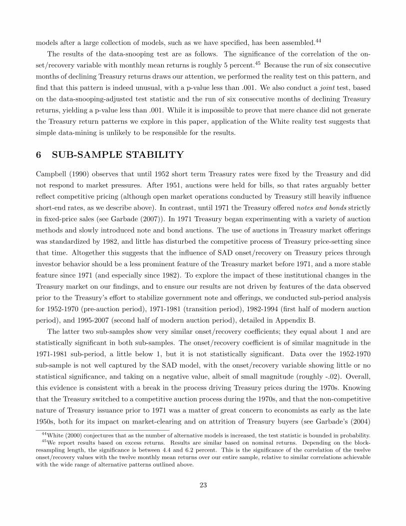
models after a large collection of models, such as we have specified, has been assembled.44

The results of the data-snooping test are as follows. The significance of the correlation of the on-

set/recovery variable with monthly mean returns is roughly 5 percent.45 Because the run of six consecutive

months of declining Treasury returns draws our attention, we performed the reality test on this pattern, and

find that this pattern is indeed unusual, with a p-value less than .001. We also conduct a joint test, based

on the data-snooping-adjusted test statistic and the run of six consecutive months of declining Treasury

returns, yielding a p-value less than .001. While it is impossible to prove that mere chance did not generate

the Treasury return patterns we explore in this paper, application of the White reality test suggests that

simple data-mining is unlikely to be responsible for the results.

6 SUB-SAMPLE STABILITY

Campbell (1990) observes that until 1952 short term Treasury rates were fixed by the Treasury and did

not respond to market pressures. After 1951, auctions were held for bills, so that rates arguably better

reflect competitive pricing (although open market operations conducted by Treasury still heavily influence

short-end rates, as we describe above). In contrast, until 1971 the Treasury offered notes and bonds strictly

in fixed-price sales (see Garbade (2007)). In 1971 Treasury began experimenting with a variety of auction

methods and slowly introduced note and bond auctions. The use of auctions in Treasury market offerings

was standardized by 1982, and little has disturbed the competitive process of Treasury price-setting since

that time. Altogether this suggests that the influence of SAD onset/recovery on Treasury prices through

investor behavior should be a less prominent feature of the Treasury market before 1971, and a more stable

feature since 1971 (and especially since 1982). To explore the impact of these institutional changes in the

Treasury market on our findings, and to ensure our results are not driven by features of the data observed

prior to the Treasury’s effort to stabilize government note and offerings, we conducted sub-period analysis

for 1952-1970 (pre-auction period), 1971-1981 (transition period), 1982-1994 (first half of modern auction

period), and 1995-2007 (second half of modern auction period), detailed in Appendix B.

The latter two sub-samples show very similar onset/recovery coefficients; they equal about 1 and are

statistically significant in both sub-samples. The onset/recovery coefficient is of similar magnitude in the

1971-1981 sub-period, a little below 1, but it is not statistically significant. Data over the 1952-1970

sub-sample is not well captured by the SAD model, with the onset/recovery variable showing little or no

statistical significance, and taking on a negative value, albeit of small magnitude (roughly -.02). Overall,

this evidence is consistent with a break in the process driving Treasury prices during the 1970s. Knowing

that the Treasury switched to a competitive auction process during the 1970s, and that the non-competitive

nature of Treasury issuance prior to 1971 was a matter of great concern to economists as early as the late

1950s, both for its impact on market-clearing and on attrition of Treasury buyers (see Garbade’s (2004)

44White (2000) conjectures that as the number of alternative models is increased, the test statistic is bounded in probability.45We report results based on excess returns. Results are similar based on nominal returns. Depending on the block-

resampling length, the significance is between 4.4 and 6.2 percent. This is the significance of the correlation of the twelveonset/recovery values with the twelve monthly mean returns over our entire sample, relative to similar correlations achievablewith the wide range of alternative patterns outlined above.

23

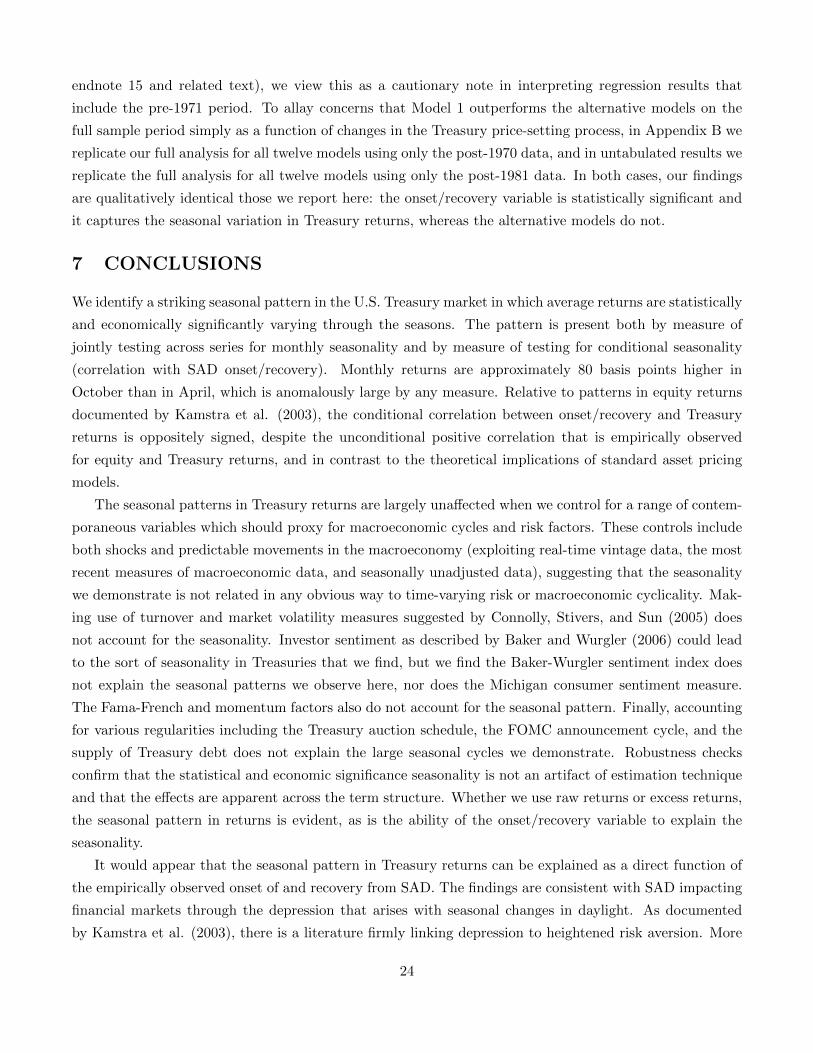
endnote 15 and related text), we view this as a cautionary note in interpreting regression results that

include the pre-1971 period. To allay concerns that Model 1 outperforms the alternative models on the

full sample period simply as a function of changes in the Treasury price-setting process, in Appendix B we

replicate our full analysis for all twelve models using only the post-1970 data, and in untabulated results we

replicate the full analysis for all twelve models using only the post-1981 data. In both cases, our findings

are qualitatively identical those we report here: the onset/recovery variable is statistically significant and

it captures the seasonal variation in Treasury returns, whereas the alternative models do not.

7 CONCLUSIONS

We identify a striking seasonal pattern in the U.S. Treasury market in which average returns are statistically

and economically significantly varying through the seasons. The pattern is present both by measure of

jointly testing across series for monthly seasonality and by measure of testing for conditional seasonality

(correlation with SAD onset/recovery). Monthly returns are approximately 80 basis points higher in

October than in April, which is anomalously large by any measure. Relative to patterns in equity returns

documented by Kamstra et al. (2003), the conditional correlation between onset/recovery and Treasury

returns is oppositely signed, despite the unconditional positive correlation that is empirically observed

for equity and Treasury returns, and in contrast to the theoretical implications of standard asset pricing

models.

The seasonal patterns in Treasury returns are largely unaffected when we control for a range of contem-

poraneous variables which should proxy for macroeconomic cycles and risk factors. These controls include

both shocks and predictable movements in the macroeconomy (exploiting real-time vintage data, the most

recent measures of macroeconomic data, and seasonally unadjusted data), suggesting that the seasonality

we demonstrate is not related in any obvious way to time-varying risk or macroeconomic cyclicality. Mak-

ing use of turnover and market volatility measures suggested by Connolly, Stivers, and Sun (2005) does

not account for the seasonality. Investor sentiment as described by Baker and Wurgler (2006) could lead

to the sort of seasonality in Treasuries that we find, but we find the Baker-Wurgler sentiment index does

not explain the seasonal patterns we observe here, nor does the Michigan consumer sentiment measure.

The Fama-French and momentum factors also do not account for the seasonal pattern. Finally, accounting

for various regularities including the Treasury auction schedule, the FOMC announcement cycle, and the

supply of Treasury debt does not explain the large seasonal cycles we demonstrate. Robustness checks

confirm that the statistical and economic significance seasonality is not an artifact of estimation technique

and that the effects are apparent across the term structure. Whether we use raw returns or excess returns,

the seasonal pattern in returns is evident, as is the ability of the onset/recovery variable to explain the

seasonality.

It would appear that the seasonal pattern in Treasury returns can be explained as a direct function of

the empirically observed onset of and recovery from SAD. The findings are consistent with SAD impacting

financial markets through the depression that arises with seasonal changes in daylight. As documented

by Kamstra et al. (2003), there is a literature firmly linking depression to heightened risk aversion. More

24

recently, Kramer and Weber (2011) study individuals who experience seasonal depression (i.e., SAD) and

a comparison group who do not. The find that SAD-sufferers are more averse to financial risk than non-

SAD-suffers, particularly so in winter, though both groups exhibited increased risk aversion in winter. This

literature provides a plausible link between the cycles evident in safe assets and those in risky securities

documented by Kamstra et al. (2003). Certainly our tests of the hypothesis that SAD onset/recovery

correlates with an annual cycle in Treasury returns result in a clear rejection of the null of no seasonality.

Use of the White (2000) reality test demonstrates that the correlation of return seasonality with the clinical

incidence of SAD symptoms unlikely to be the result of data snooping.

These findings build on other evidence consistent with time-varying risk aversion. For example, Kam-

stra, Kramer, Levi, and Wang (2011) provide theoretical foundations for the seasonal patterns in Treasury

and equity returns in an asset pricing model with time-varying risk aversion and time-varying intertempo-

ral elasticity of substitution. Further, Kamstra, Kramer, Levi, and Wermers (2011) find the flow of funds

between risky and safe categories of mutual funds varies seasonally, with funds flowing from risky to safe

categories in the fall and reversing in the spring. They study both net flows and net exchanges between

funds within a mutual fund family. We summarize the evidence from mutual fund flows in Appendix G.

We must emphasize that the seasonal pattern we find in Treasury returns does not necessarily imply

seasonal variation in risk itself. If a seasonal influence moves relatively predictably through the year in a

pattern that corresponds to the fluctuations in the clinical onset and recovery from SAD, it is unlikely that

smooth variations in risk through the course of the year are responsible. Certainly the macroeconomic

variables and asset pricing factors we control for are the most plausible sources of time-varying risk. In

spite of accounting for all of these effects, we still find remarkably strong, economically and statistically

significant evidence of a seasonal effect in Treasury returns.

25

REFERENCES

Andersen, T. G., and L. Benzoni (2010): Do Bonds Span Volatility Risk in the U.S. Treasury Market? ASpecification Test for Affine Term Structure Models, Journal of Finance, 65, 603-653, 2010.

Andersen, T.G. and L. Benzoni (2009): Realized Volatility, in Handbook of Financial Time Series, ed. byT. G. Andersen, R. A. Davis, J.-P. Kreiβ, and T. Mikosch, Berlin Heidelberg: Springer Verlag, 555-575.

Andersen, T. G., T. Bollerslev, F.X. Diebold, and P. Labys (2003): Modeling and Forecasting RealizedVolatility. Econometrica, 71(2), 529-626.

Andrews, D. W. K., and B. Lu (2001): Consistent model and moment selection procedures for GMMestimation with application to dynamic panel data models. Journal of Econometrics, 101, 123-164.

Ang, A., and M. Piazzesi (2003): A No-Arbitrage Vector Autoregression of Term Structure Dynamics withMacroeconomic and Latent Variables. Journal of Monetary Economics, 50(4), 745-787.

Baker, M., and J. Wurgler (2006): Investor sentiment and the cross-section of stock returns. Journal ofFinance, 61(4), 1645-1680.

Baker, M. and J. Wurgler (2007): Investor Sentiment in the Stock Market. Journal of Economic Perspec-tives, 21(2), 129-151.

Bekaert, G., and C. R. Harvey (1995). Time-Varying World Market Integration. Journal of Finance, 50(2),403-444.

Boudoukh, J. (1993): An Equilibrium Model of Nominal Bond Prices with Inflation-Output Correlationand Stochastic Volatility. Journal of Money, Credit, and Banking, 25(3), 636-665.

Boyd, J. H., J. Hu, and R. Jagannathan (2005): The Stock Market’s Reaction to Unemployment News:Why Bad News is Usually Good for Stocks. Journal of Finance, 60(2), 649-672.

Bracha, A., and D. Brown (2008): Affective Decision Making: A Behavioral Theory of Choice, UnpublishedManuscript, Yale University.

Brandt, M. W., and K. Q. Wang (2004): Time-Varying Risk Aversion and Unexpected Inflation. Journalof Monetary Economics, 50, 1457-1498.

Campbell, J. Y. (1990): Measuring the Persistence of Expected Returns. American Economic Review,80(2), 43-47.

Campbell, J. Y., and R. J. Shiller (1991): Yield Spreads and Interest Rate Movements: A Bird’s Eye View.Review of Economic Studies, 58(3), 495-514.

Carton, S., R. Jouvent, C. Bungenera, and D. Widlocher (1992): Sensation Seeking and Depressive Mood.Personality and Individual Differences, 13(7), 843-849.

Carton, S., P. Morand, C. Bungenera, and R. Jouvent (1995): Sensation-Seeking and Emotional Distur-bances in Depression: Relationships and Evolution, Journal of Affective Disorders, 13(3), 219-225.

Chang, E. C., and R. D. Huang (1990): Time-Varying Return and Risk in the Corporate Bond Market.Journal of Financial and Quantitative Analysis, 25(3), 323-340.

Chen, N., R. Roll, and S. A. Ross (1986): Economic Forces and the Stock Market. Journal of Business,59(3), 383-403.

Cici, G. (2005): The Relation of the Disposition Effect to Mutual Fund Trades and Performance. Unpub-lished Manuscript, University of Pennsylvania.

Cochrane, J. H. (2005): Asset Pricing, 2nd Edition. Princeton, NJ: Princeton University Press.Cochrane, J., and M. Piazzesi (2005): Bond Risk Premia. American Economic Review, 95(1), 138-160.Connolly, R., C. Stivers, and L. Sun (2005): Stock Market Uncertainty and the Stock-Bond Return Rela-

tion. Journal of Financial and Quantitative Analysis, 40(1), 161-194.De Bondt, W. F. M., and M. M. Bange (1992): Inflation Forecast Errors and Time Variation in Term

Premia. Journal of Financial and Quantitative Analysis, 27(4), 479-496.Dupont, D., and B. Sack (1999): Overview and Recent Developments. Federal Reserve Bulletin, 85,

December, 785-806.Engle, R. F. (1982): Autoregressive conditional heteroskedasticity with estimates of the variance of UK

inflation. Econometrica, 50, 987-1008.Fama, E. F., and R. Bliss (1987): The information in long-maturity forward rates. American Economic

Review, 77(4), 680-692.

26

Fama, E. F., and K. French (1993): Common Risk Factors in the Returns on Stocks and Bonds. Journalof Financial Economics, 33, 3-56.

Ferson, W., and S. Foerster (1994): Finite Sample Properties of Generalized Methods of Moments in Testsof Conditional Asset Pricing Models, Journal of Financial Economics, 36, 29-55.

Garbade K. D. (2004): The Institutionalization of Treasury Note and Bond Auctions, 1970-75. FRBNYEconomic Policy Review, 10(1), 29-45.

Garbade, K. D. (2007): The Emergence of ‘Regular and Predictable’ as a Treasury Debt ManagementStrategy. FRBNY Economic Policy Review, 13(1) 53-71.

Garrett, I., M. J. Kamstra, and L. A. Kramer (2005): Winter Blues and Time Variation in the Price ofRisk. Journal of Empirical Finance, 12(2), 291-316.

Gibson, W. E. (1970): Interest Rates and Monetary Policy, Journal of Political Economy, 78(3), 431-455.Goldreich, D. (2005): Behavioral Biases of Dealers in U.S. Treasury Auctions. Unpublished Manuscript,

University of Toronto.Godfrey, L. G. (1978a): Testing against General Autoregressive and Moving Average Error Models When

the Regressors Include Lagged Dependent Variables, Econometrica, 46, 1293-1301.Godfrey, L. G. (1978b): Testing for Higher Order Serial Correlation in Regression Equations When the

the Regressors Include Lagged Dependent Variables, Econometrica, 46, 1303-1310.Goncalves, S. and H. White (2002): ”The Bootstrap of the Mean for Dependent Heterogenous Arrays,”,

Econometric Theory, 18, 1367-1384.Goncalves, S. and H. White (2005): ”Bootstrap Standard Error Estimates for Linear Regressions,” Journal

of the American Statistical Association, 100 970-979Goyenko, R., A. Subrahmanyam, and A. Ukhov (2011): The Term Structure of Bond Market Liquidity

and its Implications for Expected Bond Returns, Journal of Financial and Quantitative Analysis, 46(1),111-139.

Hansen, L. P. (1982): Large Sample Properties of Generalized Method of Moments Estimators, Economet-rica, 50, 1029-1054.

Harmatz, M. G., A. D. Well, C. E. Overtree, K. Y. Kawamura, M. Rosal, and I S. Ockene (2000): SeasonalVariation of Depression and Other Moods: A Longitudinal Approach, Journal of Biological Rhythms,15(4), 344-350.

Harvey, C. R. (1989): Time-varying conditional covariances in tests of asset pricing models. Journal ofFinancial Economics, 24, 289-317.

Holland, A. S., and M. Toma (1991): The Role of the Federal Reserve as ”Lender of Last Resort” and theSeasonal Fluctuation of Interest Rates. Journal of Money, Credit and Banking, 23(3), 659-676.

Ilmanen, A. (1995): Time-Varying Expected Returns in International Bond Markets. Journal of Finance,50(2), 481-506.

Investment Company Institute (2008): Mutual Fund Fact Book: A Review of Trends and Activity in theMutual Fund Industry, 48th Edition.

Jegadeesh, N., and S. Titman (1993): Returns to Buying Winners and Selling Losers: Implications forStock Market Efficiency. Journal of Finance, 48, 65-91.

Jordan, S. D., and B. D. Jordan (1991): Seasonality in Daily Bond Returns. Journal of Financial andQuantitative Analysis, 26(2), 269-285.

Kamstra, M. J., L. A. Kramer, and M. D. Levi (2003): Winter Blues: A SAD Stock Market Cycle.American Economic Review, 93(1), 324-343.

Kamstra, M. J., L. A. Kramer, and M. D. Levi (2010): A Careful Re-Examination of Seasonality inInternational Stock Markets: Comment on Sentiment and Stock Returns,Available on SSRN: http://ssrn.com/abstract=1668984

Kamstra, M. J., L. A. Kramer, M .D. Levi, and T. Wang (2011): Seasonally Varying Preferences: Theo-retical Foundations for an Empirical Regularity, Unpublished Manuscript, University of Toronto.

Kamstra, M. J., L. A. Kramer, M. D. Levi, and R. Wermers (2011): Seasonal Asset Allocation: Evidencefrom Mutual Fund Flows. Available on SSRN: http://ssrn.com/abstract=1907904

Kaplanski, G., and H. Levy (2008): Seasonal Affective Disorder (SAD) and Perceived Market Risk. Un-published Manuscript, University of Jerusalem.

27

Kasper, S., T. Wehr, J. Bartko, P. Gaist, and N. Rosenthal (1989): Epidemiological Findings of SeasonalChanges in Mood and Behavior: A Telephone Survey of Montgomery County, Maryland. Archives ofGeneral Psychiatry, 46, 823-833.

Kramer, L. A., and J. M. Weber (2011): This is Your Portfolio on Winter: Seasonal Affective Disorder andRisk Aversion in Financial Decision-Making. Social Psychological and Personality Science, forthcoming.

Krishnamurthy, A. (2002): The Bond/Old-Bond Spread. Journal of Financial Economics, 66, 463-506.Krishnamurthy, A., and A. Vissing-Jorgensen (2007): The Demand for Treasury Debt. Unpublished

Manuscript, Northwestern University.Lam, R. W. (1998): Seasonal Affective Disorder: Diagnosis and Management. Primary Care Psychiatry,

4, 63-74.Lauricella, T., M. Phillips, and D. Enrich, Stocks Dive Again on Europe, Economy Fears, Wall Street

Journal, August 11, 2011.http://online.wsj.com/article/SB10001424053111904006104576500672589653988.html

Levi, M. D. (1973): Errors in the Variables Bias in the Presence of Correctly Measured Variables. Econo-metrica, 41(5), 985-986.

MacKinnon, J. G., and H. White (1985): Some Heteroskedasticity-Consistent Covariance Matrix Estima-tors with Improved Finite Sample Properties. Journal of Econometrics, 29(3), 305-325.

Newey, W. K., and K. D. West (1987): A Simple, Positive Semi-Definite, Heteroskedasticity and Autocor-relation Consistent Covariance Matrix. Econometrica, 55(3), 703-708.

Newey, W. K., and K. D. West (1994): Automatic Lag Selection in Covariance Matrix Estimation. Reviewof Economic Studies, 61, 631-653.

Palm, F. C., Smeekes, S., and Urbain, J.-P. (2008): Cross sectional dependence robust block bootstrappanel unit root tests. Maastricht, METEOR Research Memoranda 048.

Pietromonaco, P. R., and K. S. Rook (1987): Decision Style in Depression: The Contribution of PerceivedRisks Versus Benefits. Journal of Personality and Social Psychology, 52(2), 399-408.

Politis, D. N., and J. P. Romano (1994): The Stationary Bootstrap. Journal of the American StatisticalAssociation, 89(428) 1303-1313.

Rilstone, P., and M. Veall, 1996: Using Bootstrapped Confidence Intervals for Improved Inferences withSeemingly Unrelated Regression Equations Econometric Theory, 12(3), 569-580.

Schneeweis, T., and J. R. Woolridge (1979): Capital Market Seasonality: The Case of Bond Returns.Journal of Financial and Quantitative Analysis, 14(5), 939-958.

Shefrin, H. (2008): A Behavioral Approach to Asset Pricing, 2nd Edition. New York, NY: ElsevierAcademic Press.

Smoski, M. J., T. R. Lynch, M. Rosenthal, J. S. Cheavens, A. L. Chapman, and R. R. Krishnan (2008):Decision-making and risk aversion among depressive adults, Journal of Behavior Therapy, 39, 567-576.

Statman, M., K. L. Fisher, and D. Anginer. (2008): Affect in a Behavioral Asset Pricing Model, Unpub-lished Manuscript, University of Michigan.

Staiger, D., and J. H. Stock (1997): Instrumental Variables Regression with Weak Instruments, Econo-metrica, 65(3), 557-586.

Stock, J. H., and M. W. Watson (1989): New Indexes of Coincident and Leading Economic Indicators, inNBER Macroeconomics Annual, ed. by O.J. Blanchard and S. Fischer. Cambridge, MA: MIT Press.

Stock, J. H., and J. H. Wright (2000): GMM with Weak Identification. Econometrica, 68(5), 1055-1096.Terman, M. (1988): On the question of mechanism in phototherapy: considerations of clinical efficacy and

epidemiology. Journal of Biological Rhythms, 3, 155-172.Wilson, J. W., and C. P. Jones (1990): Is There a January Effect in Corporate Bond and Paper Returns?

Financial Review, 25(1), 55-71.White, H. (2000): A Reality Check for Data Snooping. Econometrica, 68(5), 1097-1126.Young, M. A., P. M. Meaden, L. F. Fogg, E. A. Cherin, and C. I. Eastman (1997): Which Environmental

Variables are Related to the Onset of Seasonal Affective Disorder? Journal of Abnormal Psychology,106(4), 554-562.

Zeng, Min, Safe Haven? Investors Still Run to Treasurys, Wall Street Journal, August 9, 2011.http://online.wsj.com/article/SB10001424053111904140604576495930871375572.html

28

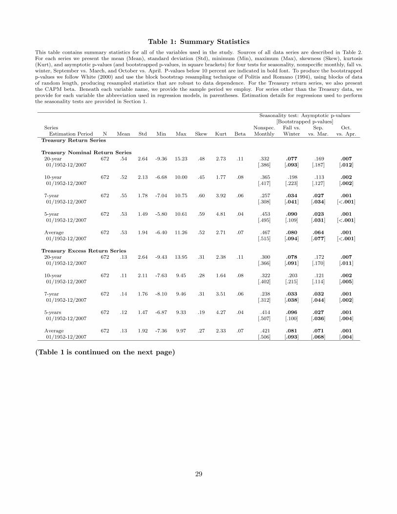
Table 1: Summary Statistics

This table contains summary statistics for all of the variables used in the study. Sources of all data series are described in Table 2.For each series we present the mean (Mean), standard deviation (Std), minimum (Min), maximum (Max), skewness (Skew), kurtosis(Kurt), and asymptotic p-values (and bootstrapped p-values, in square brackets) for four tests for seasonality, nonspecific monthly, fall vs.winter, September vs. March, and October vs. April. P-values below 10 percent are indicated in bold font. To produce the bootstrappedp-values we follow White (2000) and use the block bootstrap resampling technique of Politis and Romano (1994), using blocks of dataof random length, producing resampled statistics that are robust to data dependence. For the Treasury return series, we also presentthe CAPM beta. Beneath each variable name, we provide the sample period we employ. For series other than the Treasury data, weprovide for each variable the abbreviation used in regression models, in parentheses. Estimation details for regressions used to performthe seasonality tests are provided in Section 1.

Seasonality test: Asymptotic p-values[Bootstrapped p-values]

Series Nonspec. Fall vs. Sep. Oct.Estimation Period N Mean Std Min Max Skew Kurt Beta Monthly Winter vs. Mar. vs. Apr.

Treasury Return Series

Treasury Nominal Return Series20-year 672 .54 2.64 -9.36 15.23 .48 2.73 .11 .332 .077 .169 .00701/1952-12/2007 [.386] [.093] [.187] [.012]

10-year 672 .52 2.13 -6.68 10.00 .45 1.77 .08 .365 .198 .113 .00201/1952-12/2007 [.417] [.223] [.127] [.002]

7-year 672 .55 1.78 -7.04 10.75 .60 3.92 .06 .257 .034 .027 .00101/1952-12/2007 [.308] [.041] [.034] [<.001]

5-year 672 .53 1.49 -5.80 10.61 .59 4.81 .04 .453 .090 .023 .00101/1952-12/2007 [.495] [.109] [.031] [<.001]

Average 672 .53 1.94 -6.40 11.26 .52 2.71 .07 .467 .080 .064 .00101/1952-12/2007 [.515] [.094] [.077] [<.001]

Treasury Excess Return Series20-year 672 .13 2.64 -9.43 13.95 .31 2.38 .11 .300 .078 .172 .00701/1952-12/2007 [.366] [.091] [.170] [.011]

10-year 672 .11 2.11 -7.63 9.45 .28 1.64 .08 .322 .203 .121 .00201/1952-12/2007 [.402] [.215] [.114] [.005]

7-year 672 .14 1.76 -8.10 9.46 .31 3.51 .06 .238 .033 .032 .00101/1952-12/2007 [.312] [.038] [.044] [.002]

5-years 672 .12 1.47 -6.87 9.33 .19 4.27 .04 .414 .096 .027 .00101/1952-12/2007 [.507] [.100] [.036] [.004]

Average 672 .13 1.92 -7.36 9.97 .27 2.33 .07 .421 .081 .071 .00101/1952-12/2007 [.506] [.093] [.068] [.004]

(Table 1 is continued on the next page)

29

Table 1 (Continued)

Seasonality test: Asymptotic p-values[Bootstrapped p-values]

Series Nonspec. Fall vs. Sep. Oct.Estimation Period N Mean Std Min Max Skew Kurt Monthly Winter vs. Mar. vs. Apr.

Model 2: Treasury Debt Supply FactorsDebt-to-GDP Ratio 455 .495 .13 .31 .67 -.095 -1.71 1.000 .831 .875 .904(Debt− to−GDP ) [1.00] [.821] [.897] [.930]01/1970-11/2007

FOMC (FOMC) 456 0.75 0.43 0.00 1.00 -1.16 -0.66 .000 .002 .000 .00101/1970-12/2007 [.000] [.004] [.000] [.009]

Models 3/5: CRR Macro FactorsIndustrial Production 672 .268 .93 -3.53 6.43 .474 6.79 .962 .692 .762 .698Growth (IP ) [.338] [.566] [.352] [.262]01/1952-12/2007

Expected Inflation (Inf) 672 .310 .20 -.09 1.09 1.353 1.97 1.000 .753 .960 .63701/1952-12/2007 [1.00] [.834] [.889] [.755]

Surprise Inflation (InfSurp) 672 <.001 .24 -.94 1.40 .236 2.99 .692 .546 .268 .60101/1952-12/2007 [.583] [.358] [.338] [.787]

Default Spread (Default) 672 .934 .41 .32 2.69 1.480 2.51 .819 .805 .804 .81101/1952-12/2007 [.814] [.701] [.780] [.750]

Term Spread (Term) 672 .135 2.64 -9.43 13.95 .308 2.38 .300 .479 .457 .13101/1952-12/2007 [.295] [.526] [.493] [.292]

Models 4/5: Seasonally Unadjusted Macro VariablesInflation based on 660 .309 .34 -.80 1.81 .579 1.22 <.001 <.001 .453 .219CPI (CPISU ) [<.001] [.003] [.564] [.281]01/1952-12/2006

GDP Growth (GDPSU ) 660 .018 .03 -.11 .10 -.706 .50 <.001 <.001 <.001 <.00101/1952-12/2006 [<.001] [<.001] [<.001] [<.001]

Industrial Production 660 .003 .02 -.10 .13 -.298 1.69 <.001 <.001 .221 .001Growth (IPSU ) [.338] [.566] [.352] [.262]01/1952-12/2006

Inflation based on PPI (PPISU ) 660 .261 .72 -3.12 5.79 1.225 8.66 <.001 .002 .661 .30101/1952-12/2006 [<.001] [.003] [.564] [.281]

Unemployment Growth (USU ) 660 .005 .10 -.19 .55 1.627 3.70 <.001 <.001 .092 <.00101/1952-12/2006 [<.001] [<.001] [.107] [.004]

Model 6: Real-Time Macro VariablesUnemployment Surprise, 457 .013 .08 -.45 .69 3.101 22.18 .645 .205 .730 .941

Contraction (USurpC) [.610] [.385] [.855] [.906]12/1965-12/2003

Unemployment Surprise, 457 -.020 .17 -.64 .60 -.180 1.26 .337 .537 .948 .833Expansion (USurpE) [.610] [.385] [.855] [.906]12/1965-12/2003

Probability of 457 .158 .28 .01 .99 2.016 2.70 .849 .726 .701 .579Contraction (ProbC) [.848] [.742] [.720] [.59212/1965-12/2003

Industrial Production 457 -.107 .72 -3.53 2.14 -.816 3.06 .028 .988 .047 .084Surprise (IPSurp) [.338] [.566] [.352] [.262]12/1965-12/2003

Expected Growth in 457 .255 .33 -2.12 1.41 -1.679 11.33 .168 .317 .143 .252Industrial Production (IP ) [.168] [.359] [.172] [.255]12/1965-12/2003

Expected Change in 457 1.210 10.28 -46.81 57.26 1.175 6.28 .475 .590 .327 .485Unemployment (U) [.540] [.574] [.360] [.514]12/1965-12/2003

Change in Default 457 -.138 11.20 -66.00 55.00 -.647 7.09 .004 <.001 .344 .157Spread (∆Default) [.005] [<.001] [.369] [.159]12/1965-12/2003

Term Spread (∆Term) 457 .170 3.00 -9.43 13.95 .292 1.56 .307 .402 .213 .12012/1965-12/2003 [.295] [.526] [.493] [.292]

Inflation Surprise (InfSurp) 457 .001 .21 -.78 1.20 .454 3.09 .352 .124 .392 .92812/1965-12/2003 [.583] [.358] [.338] [.787]

Predicted Inflation (Inf) 457 .386 .23 -.06 1.34 1.295 1.63 1.000 .913 .815 .84712/1965-12/2003 [1.00] [.834] [.889] [.755]

(Table 1 is continued on the next page)

30

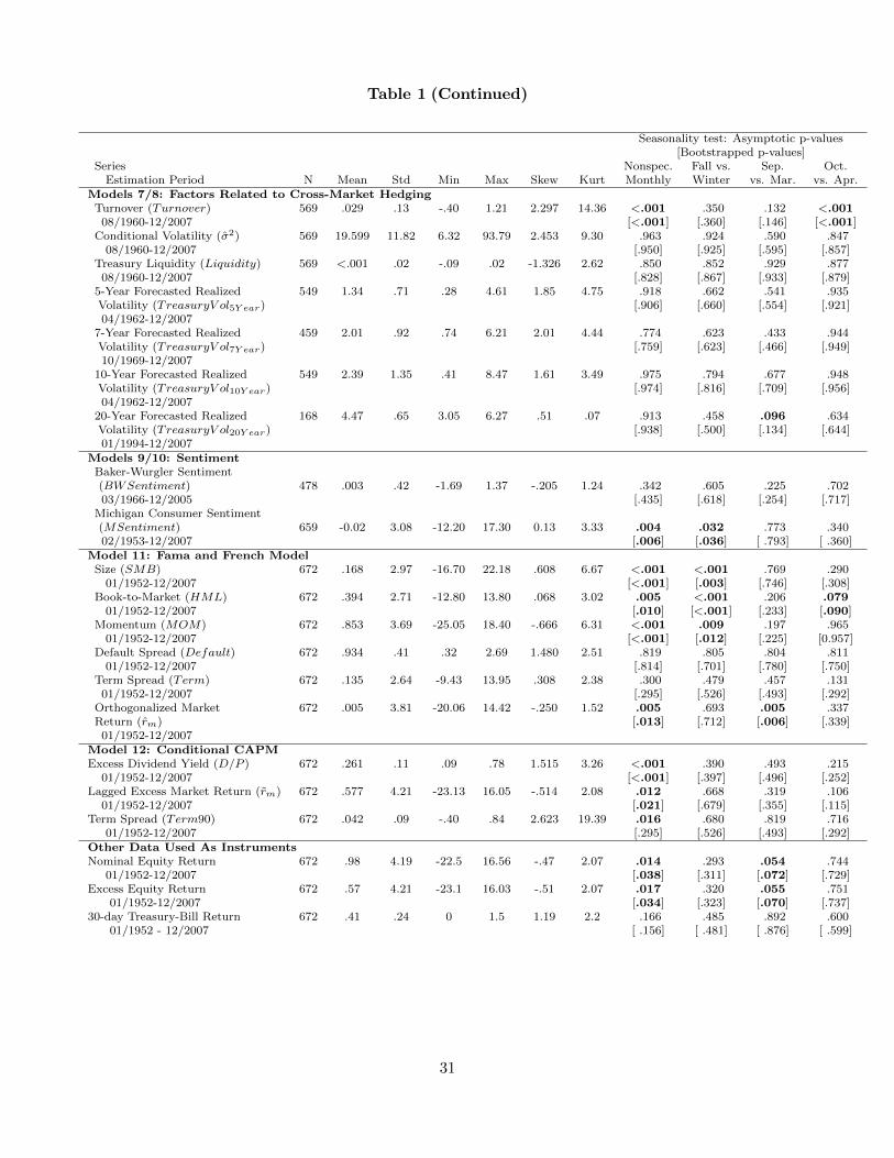
Table 1 (Continued)

Seasonality test: Asymptotic p-values[Bootstrapped p-values]

Series Nonspec. Fall vs. Sep. Oct.Estimation Period N Mean Std Min Max Skew Kurt Monthly Winter vs. Mar. vs. Apr.

Models 7/8: Factors Related to Cross-Market HedgingTurnover (Turnover) 569 .029 .13 -.40 1.21 2.297 14.36 <.001 .350 .132 <.00108/1960-12/2007 [<.001] [.360] [.146] [<.001]

Conditional Volatility (σ2) 569 19.599 11.82 6.32 93.79 2.453 9.30 .963 .924 .590 .84708/1960-12/2007 [.950] [.925] [.595] [.857]

Treasury Liquidity (Liquidity) 569 <.001 .02 -.09 .02 -1.326 2.62 .850 .852 .929 .87708/1960-12/2007 [.828] [.867] [.933] [.879]

5-Year Forecasted Realized 549 1.34 .71 .28 4.61 1.85 4.75 .918 .662 .541 .935Volatility (TreasuryV ol5Y ear) [.906] [.660] [.554] [.921]04/1962-12/2007

7-Year Forecasted Realized 459 2.01 .92 .74 6.21 2.01 4.44 .774 .623 .433 .944Volatility (TreasuryV ol7Y ear) [.759] [.623] [.466] [.949]10/1969-12/2007

10-Year Forecasted Realized 549 2.39 1.35 .41 8.47 1.61 3.49 .975 .794 .677 .948Volatility (TreasuryV ol10Y ear) [.974] [.816] [.709] [.956]04/1962-12/2007

20-Year Forecasted Realized 168 4.47 .65 3.05 6.27 .51 .07 .913 .458 .096 .634Volatility (TreasuryV ol20Y ear) [.938] [.500] [.134] [.644]01/1994-12/2007

Models 9/10: SentimentBaker-Wurgler Sentiment(BWSentiment) 478 .003 .42 -1.69 1.37 -.205 1.24 .342 .605 .225 .70203/1966-12/2005 [.435] [.618] [.254] [.717]

Michigan Consumer Sentiment(MSentiment) 659 -0.02 3.08 -12.20 17.30 0.13 3.33 .004 .032 .773 .34002/1953-12/2007 [.006] [.036] [ .793] [ .360]

Model 11: Fama and French ModelSize (SMB) 672 .168 2.97 -16.70 22.18 .608 6.67 <.001 <.001 .769 .290

01/1952-12/2007 [<.001] [.003] [.746] [.308]Book-to-Market (HML) 672 .394 2.71 -12.80 13.80 .068 3.02 .005 <.001 .206 .079

01/1952-12/2007 [.010] [<.001] [.233] [.090]Momentum (MOM) 672 .853 3.69 -25.05 18.40 -.666 6.31 <.001 .009 .197 .965

01/1952-12/2007 [<.001] [.012] [.225] [0.957]Default Spread (Default) 672 .934 .41 .32 2.69 1.480 2.51 .819 .805 .804 .811

01/1952-12/2007 [.814] [.701] [.780] [.750]Term Spread (Term) 672 .135 2.64 -9.43 13.95 .308 2.38 .300 .479 .457 .13101/1952-12/2007 [.295] [.526] [.493] [.292]

Orthogonalized Market 672 .005 3.81 -20.06 14.42 -.250 1.52 .005 .693 .005 .337Return (rm) [.013] [.712] [.006] [.339]01/1952-12/2007

Model 12: Conditional CAPMExcess Dividend Yield (D/P ) 672 .261 .11 .09 .78 1.515 3.26 <.001 .390 .493 .215

01/1952-12/2007 [<.001] [.397] [.496] [.252]Lagged Excess Market Return (rm) 672 .577 4.21 -23.13 16.05 -.514 2.08 .012 .668 .319 .106

01/1952-12/2007 [.021] [.679] [.355] [.115]Term Spread (Term90) 672 .042 .09 -.40 .84 2.623 19.39 .016 .680 .819 .716

01/1952-12/2007 [.295] [.526] [.493] [.292]Other Data Used As InstrumentsNominal Equity Return 672 .98 4.19 -22.5 16.56 -.47 2.07 .014 .293 .054 .744

01/1952-12/2007 [.038] [.311] [.072] [.729]Excess Equity Return 672 .57 4.21 -23.1 16.03 -.51 2.07 .017 .320 .055 .751

01/1952-12/2007 [.034] [.323] [.070] [.737]30-day Treasury-Bill Return 672 .41 .24 0 1.5 1.19 2.2 .166 .485 .892 .600

01/1952 - 12/2007 [ .156] [ .481] [ .876] [ .599]

31

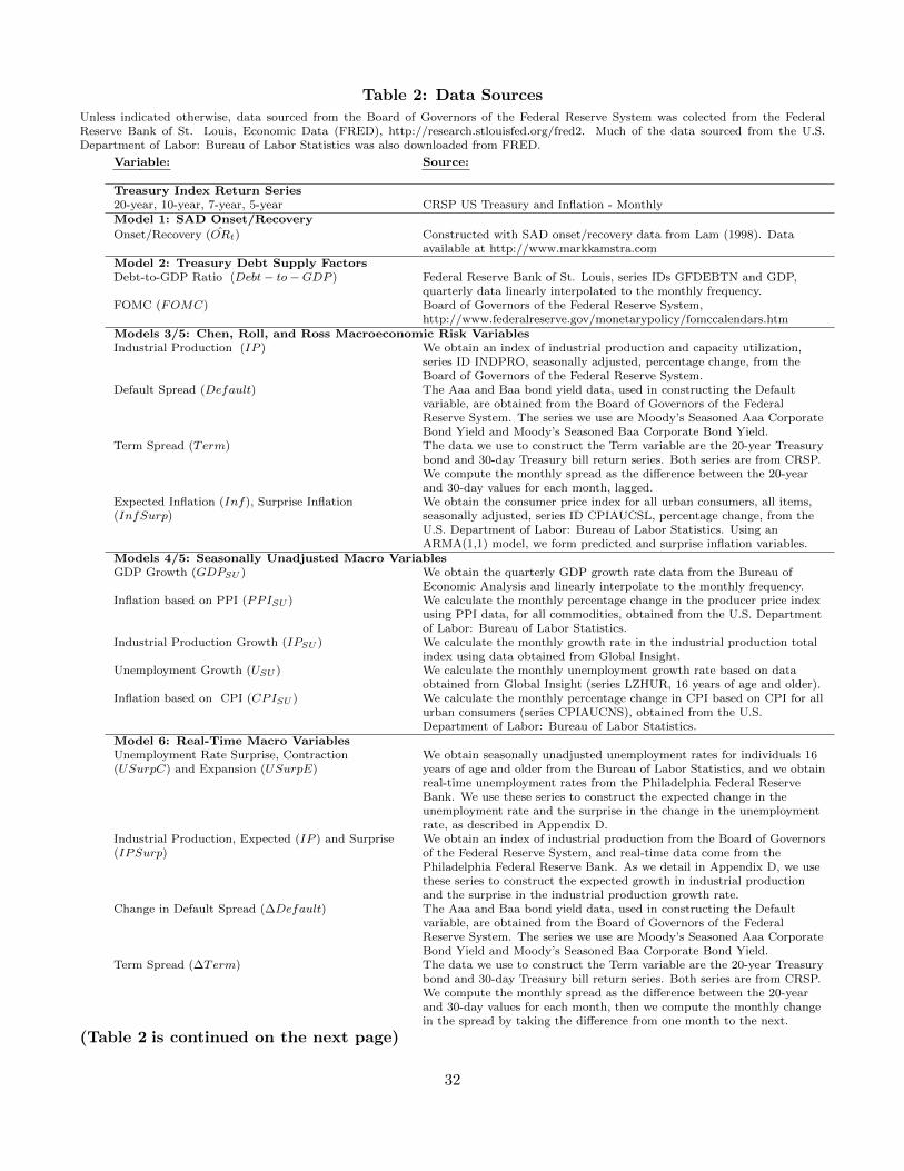
Table 2: Data Sources

Unless indicated otherwise, data sourced from the Board of Governors of the Federal Reserve System was colected from the FederalReserve Bank of St. Louis, Economic Data (FRED), http://research.stlouisfed.org/fred2. Much of the data sourced from the U.S.Department of Labor: Bureau of Labor Statistics was also downloaded from FRED.

Variable: Source:

Treasury Index Return Series20-year, 10-year, 7-year, 5-year CRSP US Treasury and Inflation - MonthlyModel 1: SAD Onset/Recovery

Onset/Recovery (ORt) Constructed with SAD onset/recovery data from Lam (1998). Dataavailable at http://www.markkamstra.com

Model 2: Treasury Debt Supply FactorsDebt-to-GDP Ratio (Debt− to−GDP ) Federal Reserve Bank of St. Louis, series IDs GFDEBTN and GDP,

quarterly data linearly interpolated to the monthly frequency.FOMC (FOMC) Board of Governors of the Federal Reserve System,

http://www.federalreserve.gov/monetarypolicy/fomccalendars.htmModels 3/5: Chen, Roll, and Ross Macroeconomic Risk VariablesIndustrial Production (IP ) We obtain an index of industrial production and capacity utilization,

series ID INDPRO, seasonally adjusted, percentage change, from theBoard of Governors of the Federal Reserve System.

Default Spread (Default) The Aaa and Baa bond yield data, used in constructing the Defaultvariable, are obtained from the Board of Governors of the FederalReserve System. The series we use are Moody’s Seasoned Aaa CorporateBond Yield and Moody’s Seasoned Baa Corporate Bond Yield.

Term Spread (Term) The data we use to construct the Term variable are the 20-year Treasurybond and 30-day Treasury bill return series. Both series are from CRSP.We compute the monthly spread as the difference between the 20-yearand 30-day values for each month, lagged.

Expected Inflation (Inf), Surprise Inflation(InfSurp)

We obtain the consumer price index for all urban consumers, all items,seasonally adjusted, series ID CPIAUCSL, percentage change, from theU.S. Department of Labor: Bureau of Labor Statistics. Using anARMA(1,1) model, we form predicted and surprise inflation variables.

Models 4/5: Seasonally Unadjusted Macro VariablesGDP Growth (GDPSU ) We obtain the quarterly GDP growth rate data from the Bureau of

Economic Analysis and linearly interpolate to the monthly frequency.Inflation based on PPI (PPISU ) We calculate the monthly percentage change in the producer price index

using PPI data, for all commodities, obtained from the U.S. Departmentof Labor: Bureau of Labor Statistics.

Industrial Production Growth (IPSU ) We calculate the monthly growth rate in the industrial production totalindex using data obtained from Global Insight.

Unemployment Growth (USU ) We calculate the monthly unemployment growth rate based on dataobtained from Global Insight (series LZHUR, 16 years of age and older).

Inflation based on CPI (CPISU ) We calculate the monthly percentage change in CPI based on CPI for allurban consumers (series CPIAUCNS), obtained from the U.S.Department of Labor: Bureau of Labor Statistics.

Model 6: Real-Time Macro VariablesUnemployment Rate Surprise, Contraction(USurpC) and Expansion (USurpE)

We obtain seasonally unadjusted unemployment rates for individuals 16years of age and older from the Bureau of Labor Statistics, and we obtainreal-time unemployment rates from the Philadelphia Federal ReserveBank. We use these series to construct the expected change in theunemployment rate and the surprise in the change in the unemploymentrate, as described in Appendix D.

Industrial Production, Expected (IP ) and Surprise(IPSurp)

We obtain an index of industrial production from the Board of Governorsof the Federal Reserve System, and real-time data come from thePhiladelphia Federal Reserve Bank. As we detail in Appendix D, we usethese series to construct the expected growth in industrial productionand the surprise in the industrial production growth rate.

Change in Default Spread (∆Default) The Aaa and Baa bond yield data, used in constructing the Defaultvariable, are obtained from the Board of Governors of the FederalReserve System. The series we use are Moody’s Seasoned Aaa CorporateBond Yield and Moody’s Seasoned Baa Corporate Bond Yield.

Term Spread (∆Term) The data we use to construct the Term variable are the 20-year Treasurybond and 30-day Treasury bill return series. Both series are from CRSP.We compute the monthly spread as the difference between the 20-yearand 30-day values for each month, then we compute the monthly changein the spread by taking the difference from one month to the next.

(Table 2 is continued on the next page)

32

Table 2 (Continued)Variable: Source:

Model 6: Real-Time Macro Variables (Continued)Probability of Contraction (ProbC) We obtain the Stock and Watson (1989) experimental coincident recession index from

the National Bureau of Economic Research. This series is a real-time indicator, makinguse of real-time information only in determining whether the economy is expanding orcontracting at a given point in time.

Inflation Surprise (InfSurp) andPredicted (Inf)

We obtain two CPI-based inflation rate series from the Philadelphia Federal ReserveBank. The first is real-time inflation, announced quarterly, available in real-timeformat only from mid-1994. The second is most recently revised inflation, availablefrom 1965. As we explain in Appendix D, we use these series to construct the inflationsurprise variable two different ways.

Models 7/8: Factors Related to Cross-Market HedgingTurnover (Turnover) Using the CRSP monthly stock file, we calculate the monthly total volume and total

shares outstanding of all stocks, form the ratio of volume to shares outstanding, thencalculate the deviation of this ratio from the (rolling) one-year average of this ratio.

Conditional Volatility (σ2) This is the fitted (conditional) value from a GARCH(1,1) model estimated on monthlyS&P 500 returns.

Treasury Liquidity (Liquidity) We form the proxy for Treasury market liquidity using proportional bid-ask spreaddata on short-term Treasury securities, maturity less than or equal to 1 year. Wefollow Goyenko et al. (2011) and adjust this measure by removing a time trend and thesquare of the time trend. We obtain the raw monthly data from the CRSP TreasuryQuotes file.

Treasury Volatility (TreasuryV ol) We calculate the volatility of daily yields for 5-year, 7-year, 10-year and 20-yearconstant maturity Treasury securities acquired from the Board of Governors of theFederal Reserve System through the St. Louis Federal Reserve, series IDs DGS5,DGS7, DGS10, and DGS20.

Models 9/10: SentimentBaker-Wurgler Sentiment(BWSentiment)

We obtain these data from Jeff Wurgler’s Web site,http://pages.stern.nyu.edu/ jwurgler/

Michigan Consumer Sentiment(MSentiment)

We obtain the Michigan consumer sentiment data from the Board of Governors of theFederal Reserve System through the St. Louis Federal Reserve, series IDs UMCSENT(mostly quarterly 11/1952 to 11/1977) and UMCSENT1 (monthly 01/1978 to01/2008). We linearly interpolate the levels of the 11/1952 to 11/1977 index tomonthly frequency, we splice the interpolated 1952-1977 monthly series with the1978-2007 monthly series, and then we calculate the monthly change. MSentimentt isdefined as the lag of the change in the monthly series.

Model 11: Fama and French ModelSize (SMB) We obtain these data from Ken French’s Web site:

http://mba.tuck.dartmouth.edu/pages/faculty/ken.french/Book-to-Market (HML) We obtain these data from Ken French’s Web site.Momentum (MOM) We obtain these data from Ken French’s Web site.Default Spread (Default) We obtain these data from Ken French’s Web site.Term Spread (Term) This is the 20-year Treasury monthly return in excess of the 30-day T-bill return,

obtained from CRSP.Orthogonalized MarketReturn (rm) We obtain these data from Ken French’s Web site.Term Spread (Term90) As defined by Harvey (1989), this is the 90-day T-bill monthly return in excess of the

30-day T-bill return, both obtained from CRSP.Model 12: Conditional CAPMExcess Dividend Yield (D/P ) This series is constructed by subtracting the CRSP equal-weighted index returns

without dividends from the CRSP equal-weighted index returns with dividends.Excess Market Return (rm) We obtain these data from Ken French’s Web site.Default Spread (Default) The Aaa and Baa bond yield data, used in constructing the Default variable, are

obtained from the Board of Governors of the Federal Reserve System. The series weuse are Moody’s Seasoned Aaa Corporate Bond Yield and Moody’s Seasoned BaaCorporate Bond Yield.

Term Spread (Term90) This is the 90-day T-bill monthly return in excess of the 30-day T-bill return, bothobtained from CRSP.

Other Data Used As InstrumentsValue-Weighted U.S. Market Return We obtain this series from CRSP. It is the NYSE/Amex/NASDAQ value-weighted

return, including distributions.30-day Treasury-Bill Return CRSP US Treasury and Inflation - Monthly

33

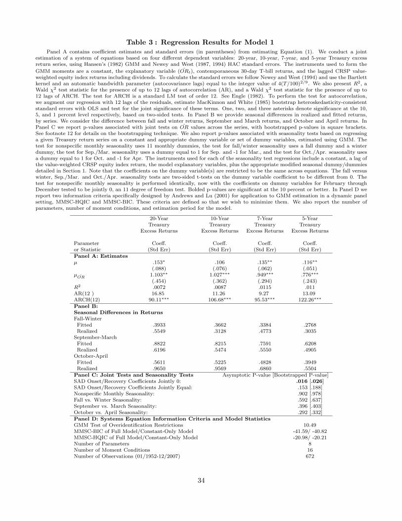
Table 3 : Regression Results for Model 1Panel A contains coefficient estimates and standard errors (in parentheses) from estimating Equation (1). We conduct a joint

estimation of a system of equations based on four different dependent variables: 20-year, 10-year, 7-year, and 5-year Treasury excessreturn series, using Hansen’s (1982) GMM and Newey and West (1987, 1994) HAC standard errors. The instruments used to form the

GMM moments are a constant, the explanatory variable (ORt), contemporaneous 30-day T-bill returns, and the lagged CRSP value-weighted equity index returns including dividends. To calculate the standard errors we follow Newey and West (1994) and use the Bartlettkernel and an automatic bandwidth parameter (autocovariance lags) equal to the integer value of 4(T/100)2/9. We also present R2, aWald χ2 test statistic for the presence of up to 12 lags of autocorrelation (AR), and a Wald χ2 test statistic for the presence of up to12 lags of ARCH. The test for ARCH is a standard LM test of order 12. See Engle (1982). To perform the test for autocorrelation,we augment our regression with 12 lags of the residuals, estimate MacKinnon and White (1985) bootstrap heteroskedasticity-consistentstandard errors with OLS and test for the joint significance of these terms. One, two, and three asterisks denote significance at the 10,5, and 1 percent level respectively, based on two-sided tests. In Panel B we provide seasonal differences in realized and fitted returns,by series. We consider the difference between fall and winter returns, September and March returns, and October and April returns. InPanel C we report p-values associated with joint tests on OR values across the series, with bootstrapped p-values in square brackets.See footnote 12 for details on the bootstrapping technique. We also report p-values associated with seasonality tests based on regressinga given Treasury return series on a constant and appropriate dummy variable or set of dummy variables, estimated using GMM. Thetest for nonspecific monthly seasonality uses 11 monthly dummies, the test for fall/winter seasonality uses a fall dummy and a winterdummy, the test for Sep./Mar. seasonality uses a dummy equal to 1 for Sep. and -1 for Mar., and the test for Oct./Apr. seasonality usesa dummy equal to 1 for Oct. and -1 for Apr. The instruments used for each of the seasonality test regressions include a constant, a lag ofthe value-weighted CRSP equity index return, the model explanatory variables, plus the appropriate modified seasonal dummy/dummiesdetailed in Section 1. Note that the coefficients on the dummy variable(s) are restricted to be the same across equations. The fall versuswinter, Sep./Mar. and Oct./Apr. seasonality tests are two-sided t-tests on the dummy variable coefficient to be different from 0. Thetest for nonspecific monthly seasonality is performed identically, now with the coefficients on dummy variables for February throughDecember tested to be jointly 0, an 11 degree of freedom test. Bolded p-values are significant at the 10 percent or better. In Panel D wereport two information criteria specifically designed by Andrews and Lu (2001) for application to GMM estimation in a dynamic panelsetting, MMSC-HQIC and MMSC-BIC. These criteria are defined so that we wish to minimize them. We also report the number ofparameters, number of moment conditions, and estimation period for the model.

20-Year 10-Year 7-Year 5-YearTreasury Treasury Treasury Treasury

Excess Returns Excess Returns Excess Returns Excess Returns

Parameter Coeff. Coeff. Coeff. Coeff.or Statistic (Std Err) (Std Err) (Std Err) (Std Err)Panel A: Estimatesµ .153∗ .106 .135∗∗ .116∗∗

(.088) (.076) (.062) (.051)µOR 1.103∗∗ 1.027∗∗∗ .949∗∗∗ .776∗∗∗

(.454) (.362) (.294) (.243)R2 .0072 .0087 .0115 .011AR(12 ) 16.85 11.26 9.27 13.09ARCH(12) 90.11∗∗∗ 106.68∗∗∗ 95.53∗∗∗ 122.26∗∗∗

Panel B:Seasonal Differences in ReturnsFall-Winter

Fitted .3933 .3662 .3384 .2768Realized .5549 .3128 .4773 .3035

September-MarchFitted .8822 .8215 .7591 .6208Realized .6196 .5474 .5550 .4905

October-AprilFitted .5611 .5225 .4828 .3949Realized .9650 .9569 .6860 .5504

Panel C: Joint Tests and Seasonality Tests Asymptotic P-value [Bootstrapped P-value]SAD Onset/Recovery Coefficients Jointly 0: .016 [.026]SAD Onset/Recovery Coefficients Jointly Equal: .153 [.188]Nonspecific Monthly Seasonality: .902 [.978]Fall vs. Winter Seasonality: .592 [.637]September vs. March Seasonality: .396 [.403]October vs. April Seasonality: .292 [.332]Panel D: Systems Equation Information Criteria and Model StatisticsGMM Test of Overidentification Restrictions 10.49MMSC-BIC of Full Model/Constant-Only Model -41.59/ -40.82MMSC-HQIC of Full Model/Constant-Only Model -20.98/ -20.21Number of Parameters 8Number of Moment Conditions 16Number of Observations (01/1952-12/2007) 672

34

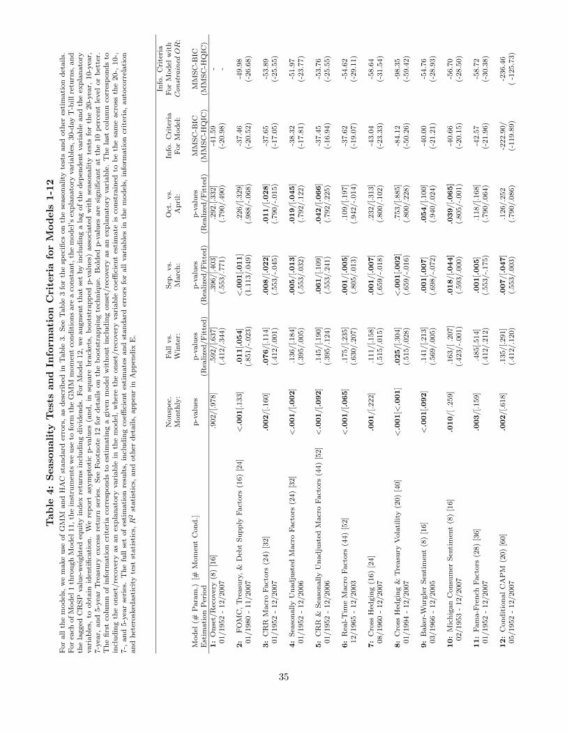
Tab

le4:

Seaso

nality

Test

san

dIn

form

ati

on

Cri

teri

afo

rM

od

els

1-1

2F

or

all

the

mod

els,

we

make

use

of

GM

Man

dH

AC

stan

dard

erro

rs,

as

des

crib

edin

Tab

le3.

See

Tab

le3

for

the

spec

ifics

on

the

seaso

nality

test

san

doth

eres

tim

ati

on

det

ails.

For

each

of

Mod

el1

thro

ugh

Mod

el11,

the

inst

rum

ents

we

use

tofo

rmth

eG

MM

mom

ent

con

dit

ion

sare

aco

nst

ant,

the

mod

el’s

exp

lan

ato

ryvari

ab

les,

30-d

ay

T-b

illre

turn

s,an

dth

ela

gged

CR

SP

valu

e-w

eighte

deq

uit

yin

dex

retu

rns

incl

ud

ing

div

iden

ds.

For

Mod

el12,

we

au

gm

ent

that

set

by

incl

ud

ing

ala

gof

the

dep

end

ent

vari

ab

lean

dth

eex

pla

nato

ryvari

ab

les,

toob

tain

iden

tifi

cati

on

.W

ere

port

asy

mp

toti

cp

-valu

es(a

nd

,in

squ

are

bra

cket

s,b

oots

trap

ped

p-v

alu

es)

ass

oci

ate

dw

ith

seaso

nali

tyte

sts

for

the

20-y

ear,

10-y

ear,

7-y

ear,

an

d5-y

ear

Tre

asu

ryex

cess

retu

rnse

ries

.S

eeF

ootn

ote

12

for

det

ails

on

the

boots

trap

pin

gte

chn

iqu

e.B

old

edp

-valu

esare

sign

ifica

nt

at

the

10

per

cent

level

or

bet

ter.

Th

efi

rst

colu

mn

of

info

rmati

on

crit

eria

corr

esp

on

ds

toes

tim

ati

ng

agiv

enm

od

elw

ith

ou

tin

clu

din

gon

set/

reco

ver

yas

an

exp

lan

ato

ryvari

ab

le.

Th

ela

stco

lum

nco

rres

pon

ds

toin

clu

din

gth

eon

set/

reco

ver

yas

an

exp

lan

ato

ryvari

ab

lein

the

mod

el,

wh

ere

the

on

set/

reco

ver

yvari

ab

leco

effici

ent

esti

mate

isco

nst

rain

edto

be

the

sam

eacr

oss

the

20-,

10-,

7-,

an

d5-y

ear

seri

es.

Th

efu

llse

tof

esti

mati

on

resu

lts,

incl

ud

ing

coeffi

cien

tes

tim

ate

sand

stan

dard

erro

rsfo

rall

vari

ab

les

inth

em

od

els,

info

rmati

on

crit

eria

,au

toco

rrel

ati

on

an

dh

eter

osk

edast

icit

yte

stst

ati

stic

s,R

2st

ati

stic

s,an

doth

erdet

ail

s,ap

pea

rin

Ap

pen

dix

E.

Info

.C

rite

ria

Non

spec

.F

all

vs.

Sep

.vs.

Oct

.vs.

Info

.C

rite

ria

For

Mod

elw

ith

Month

ly:

Win

ter:

Marc

h:

Ap

ril:

For

Mod

el:

ConstrainedOR

:

Mod

el(#

Para

m.)

[#M

om

ent

Con

d.]

p-v

alu

esp

-valu

esp

-valu

esp

-valu

esM

MS

C-B

ICM

MS

C-B

ICE

stim

ati

on

Per

iod

(Rea

lize

d/F

itte

d)

(Rea

lize

d/F

itte

d)

(Rea

lize

d/F

itte

d)

(MM

SC

-HQ

IC)

(MM

SC

-HQ

IC)

1:

On

set/

Rec

over

y(8

)[1

6]

.902/[.978]

.592/[.637]

.396/[.403]

.292.[.3

32]

-41.5

9-

01/1952

-12/2007

(.412/.3

44)

(.553/.7

71)

(.790/.4

90)

(-20.9

8)

-

2:

FO

MC

,T

reasu

ry,

&D

ebt

Su

pp

lyF

act

ors

(16)

[24]

<.0

01

[.133]

.011

[.054

]<

.001

[.011

].2

26/[.329]

-37.4

6-4

9.9

801/1980

-11/2007

(.851/-.

023)

(1.1

13/.0

49)

(.988/-.

068)

(-20.5

2)

(-26.6

8)

3:

CR

RM

acr

oF

act

ors

(24)

[32]

.002

/[.160]

.076

/[.114]

.008

/[.022

].0

11

/[.028

]-3

7.6

5-5

3.8

901/1952

-12/2007

(.412/.0

01)

(.553/-.

045)

(.790/-.

015)

(-17.0

5)

(-25.5

5)

4:

Sea

son

ally

Un

ad

just

edM

acr

oF

act

ors

(24)

[32]

<.0

01

/[.002

].1

36/[.184]

.005

/[.013

].0

19

/[.045

]-3

8.3

2-5

1.9

701/1952

-12/2006

(.395/.0

05)

(.553/.0

32)

(.792/.1

22)

(-17.8

1)

(-23.7

7)

5:

CR

R&

Sea

son

ally

Un

ad

just

edM

acr

oF

act

ors

(44)

[52]

<.0

01

/[.092

].1

45/[.190]

.061

/[.109]

.042

/[.066

]-3

7.4

5-5

3.7

601/1952

-12/2006

(.395/.1

24)

(.553/.2

41)

(.792/.2

25)

(-16.9

4)

(-25.5

5)

6:

Rea

l-T

ime

Macr

oF

act

ors

(44)

[52]

<.0

01

/[.065

].1

75/[.235]

.001

/[.005

].1

09/[.197]

-37.6

2-5

4.6

212/1965

-12/2003

(.630/.2

07)

(.805/.0

13)

(.942/-.

014)

(-19.0

7)

(-29.1

1)

7:

Cro

ssH

edgin

g(1

6)

[24]

.001

/[.222]

.111/[.158]

.001

/[.007

].2

32/[.313]

-43.0

4-5

8.6

408/1960

-12/2007

(.515/.0

15)

(.659/-.

018)

(.800/.1

02)

(-23.3

3)

(-31.5

4)

8:

Cro

ssH

edgin

g&

Tre

asu

ryV

ola

tility

(20)

[40]

<.0

01

[<.0

01

].0

25

/[.304]

<.0

01

[.002

].7

53/[.885]

-84.1

2-9

8.3

501/1994

-12/2007

(.515/.0

28)

(.659/-.

016)

(.800/.2

28)

(-50.2

6)

(-59.4

2)

9:

Baker

-Wu

rgle

rS

enti

men

t(8

)[1

6]

<.0

01

[.092

].1

41/[.213]

.001

[.007

].0

54

/[.100]

-40.0

0-5

4.7

603/1966

-12/2005

(.569/.0

05)

(.698/-.

072)

(.940/.0

24)

(-21.2

1)

(-28.9

3)

10:

Mic

hig

an

Con

sum

erS

enti

men

t(8

)[1

6]

.010

/[

.259]

.163/[

.207]

.018

/[.044]

.039

/[.065]

-40.6

6-5

6.7

002/1953

-12/2007

(.423/-.

001)

(.593/.0

00)

(.805/-.

001)

(-20.1

5)

(-28.5

0)

11:

Fam

a-F

ren

chF

act

ors

(28)

[36]

.003

/[.159]

.485[.514]

.001

[.005

].1

18/[.168]

-42.5

7-5

8.7

201/1952

-12/2007

(.412/.2

12)

(.553/-.

175)

(.790/.0

64)

(-21.9

6)

(-30.3

8)

12:

Con

dit

ion

al

CA

PM

(20)

[60]

.002

/[.618]

.135/[.291]

.007

/[.047

].1

26/.2

52

-222.9

0/

-236.4

605/1952

-12/2007

(.412/.1

20)

(.553/.0

03)

(.790/.0

86)

(-119.8

9)

(-1

25.7

3)

35

Table 5: Coefficient Estimates on the Onset/Recovery VariableEmbedded within Models 1 - 12

In the first four columns we report coefficient estimates and standard errors (in parentheses) for the onset/recovery variable (ORt)from estimating Equation (1) as well as versions of Equations (2) through (12) that have been modified to include the onset/recoveryvariable as an additional explanatory variable, with no restriction that the onset/recovery coefficient estimates be equal across series fora given model. We conduct a joint estimation of each system of equations based on four different dependent variables: 20-year, 10-year,7-year, and 5-year Treasury excess return series, using Hansen’s (1982) GMM and Newey and West (1987) HAC standard errors. Tocalculate the standard errors we follow Newey and West (1994) and use the Bartlett kernel and an automatic bandwidth parameter(autocovariance lags) equal to the integer value of 4(T/100)2/9. For each of Model 1 and Model 2′ through Model 11′, the instruments weuse to form the GMM moment conditions are a constant, the model’s explanatory variables, 30-day T-bill returns, and the lagged CRSPvalue-weighted equity index returns including dividends. For Model 12′, we augment that set by including a lag of the dependent variableand the explanatory variables, to obtain identification. In the fifth column we report asymptotic p-values (and, in square brackets,bootstrapped p-values) associated with tests that the coefficient estimates on the onset/recovery variable are jointly equal to zero (orjointly equal to each other, beneath). See Footnote 12 for details on the bootstrapping technique. Sample estimation periods appearunder each model label. For coefficient estimates, one, two, and three asterisks denote significance at the 10, 5, and 1 percent levelrespectively, based on two-sided tests. Bolded p-values associated with joint tests are significant at the 10 percent level or better. Fullregression results for each model appear in Appendix F.

P-values for20-Year 10-Year 7-Year 5-Year ParameterTreasury Treasury Treasury Treasury Joint Tests

Excess Returns Excess Returns Excess Returns Excess Returns Asymptotic/[Bootstrapped]

Model Coeff. Coeff. Coeff. Coeff. Jointly 0Estimation Period (Std Err) (Std Err) (Std Err) (Std Err) (Jointly Equal)

1: Onset/Recovery 1.103∗∗ 1.027∗∗∗ .949∗∗∗ .776∗∗∗ .016/[.026]01/1952 - 12/2007 (.454) (.362) (.294) (.243) (.153/[.188])

2′: FOMC, Treasury, &Debt Supply Factors 2.437∗∗∗ 2.077∗∗∗ 1.704∗∗∗ 1.430∗∗∗ .003/[.016]01/1980 - 11/2007 (.773) (.570) (.467) (.383) (.051/[.076])

3′: CRR Macro Factors 1.270∗∗∗ 1.114∗∗∗ 1.039∗∗∗ .858∗∗∗ .003/[.004]01/1952 - 12/2007 (.428) (.336) (.271) (.226) (.126/[.154])

4′: Seasonally UnadjustedMacro Factors 1.624∗∗∗ 1.920∗∗∗ 1.599∗∗∗ 1.377∗∗∗ <.001/[<.001]01/1052 - 12/2006 (.561) (.461) (.368) (.315) (.026/[.041])

5′: CRR & SeasonallyUnadjusted Macro Factors 1.284∗∗ 1.620∗∗∗ 1.360∗∗∗ 1.207∗∗∗ <.001/[.002]01/1952 - 12/2006 (.593) (.486) (.386) (.333) (.090/[.123])

6′: Real-Time Macro Factors 1.470∗∗ 1.399∗∗∗ 1.240∗∗∗ 1.057∗∗∗ .004/[.009]12/1965 - 12/2003 (.643) (.479) (.380) (.314) (.306)/[.330]

7′: Cross Hedging 1.416∗∗∗ 1.265∗∗∗ 1.154∗∗∗ .970∗∗∗ .008/[.011]08/1960 - 12/2007 (.532) (.420) (.335) (.281) (.177/[.207])

8′: Cross Hedging &Treasury Volatility 2.347∗∗∗ 1.786∗∗∗ 1.386∗∗∗ 1.021∗∗∗ .059/[.408]01/1994 - 12/2007 (.809) (.608) (.489) (.379) (.030/[.232])

9′: Baker-Wurgler Sentiment 1.562∗∗ 1.520∗∗∗ 1.346∗∗∗ 1.133∗∗∗ .003/[.005]03/1966 - 12/2005 (.620) (.481) (.391) (.327) (.122/[.148])

10′: Michigan ConsumerSentiment 1.171∗∗ 1.082∗∗∗ .987∗∗∗ .807∗∗∗ .020/[.026]02/1953 - 12/2007 ( .471) (.375) (.307) (.256) (.144/[.163])

11′: Fama-French Factors 1.019∗∗ .933∗∗∗ .818∗∗∗ .706∗∗∗ .040/[.05]01/1952 - 12/2007 (.446) (.345) (.279) (.231) (.503/[.534])

12′ Conditional CAPM 8.160 11.646∗∗ 9.405∗∗∗ 11.874∗∗ .024/[.034]01/1952 - 12/2007 (6.363) (5.493) (2.923) (5.505) (.737/[.754])

36