Transportation Research Part B 45 (2011) 605–617

Contents lists available at ScienceDirect

Transportation Research Part B

journal homepage: www.elsevier .com/ locate/ t rb

Properties of a well-defined macroscopic fundamental diagramfor urban traffic

Nikolas Geroliminis a,⇑, Jie Sun b

a Urban Transport Systems Laboratory, School of Architecture, Civil and Environmental Engineering, Ecole Polytechnique Fédérale de Lausanne (EPFL), Switzerlandb Department of Civil Engineering, University of Minnesota, Twin Cities, USA

a r t i c l e i n f o

Article history:Received 3 January 2010Received in revised form 6 November 2010Accepted 6 November 2010

Keywords:CongestionUrban trafficMacroscopic modelingArterialsHysteresis

0191-2615/$ - see front matter � 2010 Elsevier Ltddoi:10.1016/j.trb.2010.11.004

⇑ Corresponding author. Tel.: +41 21 69 32481.E-mail addresses: nikolas.geroliminis@epfl.ch (N

a b s t r a c t

A field experiment in Yokohama (Japan) revealed that a macroscopic fundamental diagram(MFD) linking space-mean flow, density and speed exists on a large urban area. It wasobserved that when the highly scattered plots of flow vs. density from individual fixeddetectors were aggregated the scatter nearly disappeared and points grouped along a welldefined curve. Despite these and other recent findings for the existence of well-definedMFDs for urban areas, these MFDs should not be universally expected. In this paper weinvestigate what are the properties that a network should satisfy, so that an MFD withlow scatter exists. We show that the spatial distribution of vehicle density in the networkis one of the key components that affect the scatter of an MFD and its shape. We also pro-pose an analytical derivation of the spatial distribution of congestion that considers corre-lation between adjacent links. We investigate the scatter of an MFD in terms of errors in theprobability density function of spatial link occupancy and errors of individual links’ funda-mental diagram (FD). Later, using real data from detectors for an urban arterial and a free-way network we validate the proposed derivations and we show that an MFD is not welldefined in freeway networks as hysteresis effects are present. The datasets in this paperconsist of flow and occupancy measures from 500 fixed sensors in the Yokohama down-town area in Japan and 600 loop detectors in the Twin Cities Metropolitan Area Freewaynetwork in Minnesota, USA.

� 2010 Elsevier Ltd. All rights reserved.

1. Introduction

This paper is to search for the properties of the macroscopic modeling of traffic flow under congested conditions. Theunderstanding of these properties should be the first step to macroscopic modeling-based alternative traffic managementschemes, such as pricing and perimeter control to mitigate congestion and improve mobility in urban areas.

It has been recently proposed and tested in Daganzo (2007) and Geroliminis and Daganzo (2007, 2008), that traffic inlarge urban regions can be modeled dynamically at an aggregate level, if the neighborhoods are uniformly congested. Thelast two papers showed, using a micro-simulation of the San Francisco Business district and a field experiment in downtownYokohama (Japan), (i) that urban neighborhoods approximately exhibit a ‘‘macroscopic fundamental diagram’’ (MFD) relat-ing the number of vehicles (accumulation) in the neighborhood to the neighborhood’s average speed (or flow) and (ii) thereis a robust linear relation between the neighborhood’s average flow and its total outflow (rate vehicles reach their destina-tions). The experiment used a combination of fixed detectors and floating vehicle probes as sensors. It was also observed thatwhen the somewhat chaotic scatter-plots of speed vs. density from individual fixed detectors were aggregated for a

. All rights reserved.

. Geroliminis), sunxx308@umn.edu (J. Sun).

606 N. Geroliminis, J. Sun / Transportation Research Part B 45 (2011) 605–617

downtown region around 10 km2, the scatter nearly disappeared and points grouped neatly along a smoothly decliningcurve. The same references also showed that (a) the MFD is a property of the network itself (infrastructure and control)and not of the demand, i.e. the MFD should have a well-defined maximum and remain invariant when the demand changesboth with the time-of-day and across days; (b) the space-mean flow, is maximum for the same value of density of vehicles oraverage speed, independent of the origin–destination tables; (c) the average trip length for the study region is about constantwith time, i.e. the total outflow vs. density curve is a scaled up version of the average network flow vs. density curve; and (d)the MFD can be estimated accurately using existing monitoring technologies (e.g. detector data, GPS, etc.).

The idea of an MFD with an optimum accumulation is quite old and belongs to Godfrey (1969), but the verification of itsexistence with dynamic features is recent (Geroliminis and Daganzo, 2007, 2008). Earlier works had looked for MFD patternsin data from lightly congested real-world networks (Godfrey, 1969; Ardekani and Herman, 1987; Olszewski et al., 1995) or indata from simulations with artificial routing rules and static demands (Mahmassani et al., 1987; Williams et al., 1987;Mahmassani and Peeta, 1993) but the data from all these studies were too sparse or not investigated deeply enough to dem-onstrate that an invariant MFD could dynamically arise in the real world. Although Geroliminis and Daganzo (2007, 2008)have shown that this can indeed happen, more real-world experiments should shed light on the types of networks anddemand conditions for which invariant MFD’s arise. Invariance is important because knowledge of a neighborhood’s MFDallows decision-makers to use demand-side policies to improve mobility. However, to evaluate changes to the network(e.g., re-timing the traffic signals or allocating the percentage of streets devoted to public transit) one needs to know howthe MFD is affected by these changes. To this end, Daganzo and Geroliminis (2008) explored the connection between net-work structure and a network’s MFD for urban neighborhoods with cars controlled by traffic signals. Helbing (2009) has alsoderived analytical theories for an MFD, using a utilization-based approach.

Despite these recent findings for the existence of well-defined MFDs for urban areas, these MFDs should not be univer-sally expected. The framework of an MFD was proposed under the assumption that congestion is evenly distributed, i.e. theareas with an MFD should be (roughly) homogeneously loaded (Daganzo, 2007; Geroliminis and Daganzo, 2007, 2008). Awell-defined MFD was observed in the last two references, but the homogeneity assumption was not deeply explored. In thispaper we provide a clearer understanding of the spatial distribution of vehicles in a network and how these affect the scatterand the existence of an MFD. This paper demonstrates with real data that a strict homogeneity of traffic states on the net-work, as initially conjectured by Daganzo (2007), is not necessary to observe a well-defined MFD.

To this end we define as Aggregated Traffic Relationship (ATR), a relationship between average traffic variables (likespeed, density, occupancy or flow) for a specific network that not necessarily have a well defined shape to be called anMFD. In particular, networks with an uneven and inconsistent distribution of congestion may exhibit traffic states thatare well below the upper bound of an ATR and much too scattered to line along an MFD. An inconsistent distribution of con-gestion is typical of freeway networks with multiple recurrent and non-recurrent bottlenecks, and of large urban areas withmultiple congested sub-centers. Even networks that satisfy some of the regularity conditions pointed above may exhibit sig-nificant scatter on their MFDs because of a rapidly changing demand, e.g. during an emergency evacuation an MFD may notexist for an urban network which exhibits an MFD under normal conditions.

The effect of heterogeneity in ATRs or MFDs has been experimentally examined to some aspects with real data from amedium-size French city by Buisson and Ladier (2009). The authors examined differences between the arterial and freewaynetwork, impact of the distance between the loop detector and the traffic signal within the urban network, differences be-tween normal and non-recurring conditions (during a strike of truck drivers). They showed that heterogeneity has a strongimpact on the shape/scatter of an MFD, that may turn not to be an MFD in some cases, e.g. for a freeway network. In parallelwith our work, Daganzo et al. (2011) investigated bifurcations and instability issues in an MFD for a two-ring network.

In this paper we investigate what are the properties that a network should satisfy, so that an MFD with low scatter exists.The remainder of this paper is organized as follows: Firstly, we show that the spatial distribution of car density in the net-work is one of the key components that affect the scatter of an MFD and its shape. We also propose an analytical derivation ofthe spatial distribution that considers correlation between adjacent links. We investigate the scatter of an MFD in terms oferrors in probability density function of spatial occupancy and errors of individual links’ fundamental diagram (FD). Later,

2km 5km

Fig. 1. Test sites: (left) Yokohama downtown arterial network; (right) Minneapolis, Twin Cities freeway network.

N. Geroliminis, J. Sun / Transportation Research Part B 45 (2011) 605–617 607

using real data from detectors for an urban arterial and a freeway network we validate the proposed derivations and weshow that an MFD is not well defined in freeway networks as hysteresis effects are present.

The datasets in this paper consist of flow and occupancy measures from 500 fixed sensors in the Yokohama downtownarea and 600 loop detectors in the Twin Cities Metropolitan Area Freeway network (Minnesota, USA). Fig. 1 illustrates thetest sites used in the paper.

2. Properties of a well-defined MFD

A macroscopic fundamental diagram (MFD) linking space-mean flow, density and speed has been observed in Yokohama,Japan through a field experiment (Geroliminis and Daganzo, 2008). The relation between space-mean flows on the wholenetwork and the trip completion rates was also explored there, but not how the spatial variability of link vehicle densityaffects the shape of the MFD or even its existence. In this section, we first explore the spatial distribution of individual detec-tor occupancy for different times of day, which is a metric of the spatial distribution of vehicles in the network.

2.1. Occupancy distributions

The framework of an MFD was proposed under the assumption that congestion is evenly distributed, i.e. the homogeneityassumption of the MFD (Daganzo, 2007; Geroliminis and Daganzo, 2007, 2008). A well-defined MFD was observed in the lasttwo references, but the homogeneity assumption was not deeply explored. In this section, we try to shed some light to thisdirection and develop a metric to test the range of the spatial heterogeneity of congestion for a well-defined MFD.

The data of a typical workday (12/14/2001) is chosen, which is consistent with the previous test in Yokohama. Our rawdata is in form of volume and occupancy, which come directly from loop detectors and some obvious errors/malfunctions(e.g. data with occupancy over 100 or stay 0 for all times) are eliminated before analyzing the data. One can see from thetime series plot of average network occupancy, O, for the study site of Fig. 1a, that the network is almost empty at the begin-ning of the day with average occupancy close to zero. There are two dense peak times during the day: morning peak andevening peak, when the average occupancy would reach as high as almost 50%.

Let us index the road lane section between two intersections as d, and let qd and od donate the flow and occupancy mea-sured by the detector during a time slice on this specific road lane section. It is known that the density k in the proximity of adetector can be given by od

s , where s is the effective vehicle length, which can be considered as a parameter of a specific net-work. The weighted average (using link lengths) of occupancy could be space-mean for the network if the detectors happento be at representative locations within each link. This should happen automatically for flows on time slices large comparedwith a signal cycle because on this time scale link flows are roughly the same regardless of where they are measured within alink. But obviously, the same is not necessarily true for density. We continue our analysis using occupancy measures, as theyare directly available.1

Let O be the average network occupancy in the proximity of all detectors during time interval t (comparable in size withone signal cycle), and Q be the average flow of all detectors during the same time interval (interval t is omitted from thenotation for simplicity purposes). We have to note that Q and O in our analysis are unweighted averages, which may con-tradict the generalized definitions of network flow and density according to (Edie, 1963), where weighted averages usingthe length of individual links are estimated. Actually, Geroliminis and Daganzo (2008) showed for the Yokohama test site,that both the weighted and unweighted averages produce a well-defined MFD with similar scatter. Thus, we focus our anal-ysis in a simpler definition.

We now test the following conjecture: If the spatial distribution of link occupancy is the same for two different time inter-vals with the same average network occupancy then these two time intervals should have the same average flows, i.e. in anMFD plane these two are points close to each other. Mathematically speaking, if we estimate the probability density functiondr(t), of all individual detectors’ at a specific time t, in region r, and the average network flow and occupancy, Q(t) and O(t), awell-defined MFD exists in r when for all t1, t2 we have:

1 Usifor the

fQðt1Þ ¼ Qðt2Þ and Oðt1Þ ¼ Oðt2Þg () drðt1Þ � drðt2Þ:

To test the conjecture for a wide range of traffic conditions from uncongested to heavily congested, we choose an averageoccupancy of 15%, 25%, 35% and 45%. We look at all times during a day that O is close to these values, e.g. for O = 35% the timepoints that the dashed line intersects with the occupancy time series in Fig. 2. For each average occupancy level, we collectfive time intervals whose differences in O are less than 1% and we plot the histograms for each average occupancy group(shown in Fig. 3). We discretize the full occupancy range from 0% to 100% in 23 groups; one group for empty links with zerooccupancy and 22 groups of equal range. The value 22 is the maximum number of vehicles for a link N = kjam � l, where theaverage link length and the jam density for the study site are estimated to be l = 154 m and kjam = 0.14 veh/m (Daganzo andGeroliminis, 2008).

ng mid-block detector data Geroliminis and Daganzo (2008) found that the weighted and unweighted values of average network occupancy are similarcity of Yokohama and that O

s provides a decent approximation of the average network density (errors less than 15%).

O(%

)Fig. 2. Time series of average network occupancy for the day of December 14, 2001 in downtown Yokohama.

Prob

abili

ty

Occ. Group

O 15%

Prob

abili

ty

Occ. Group

O 25%

Prob

abili

ty

Occ. Group

O 35%

Prob

abili

ty

Occ. Group

O 45%

Fig. 3. Histograms for different values of average occupancy in the arterial network, O (Occupancy group #1 represents empty links (O = 0), groups #2–#23have a range of occupancy equal to 100%/22 = 4.55%).

608 N. Geroliminis, J. Sun / Transportation Research Part B 45 (2011) 605–617

It is very clear from these graphs that congestion is not evenly distributed. Some parts of the network are more congestedthan others. As more parts of the network become congested, the distribution of detector occupancy is shifted to the right.Note that the distributions of occupancy with similar average occupancy are similar although they come from different timeintervals.

2.2. Statistical analysis

Some statistical tools are needed for our investigation into the property of the individual detector occupancy distribu-tions. The two major statistical tests we are using in this paper are the Chi-square test and the Mann–Whitney U test.

The kind of Chi-square test we are using in this paper is called Pearson’s chi-square test. It is used to test whether thesample distribution of a categorical variable is different from a population with a hypothesized distribution or not and

Table 1Results from statistical tests for occupancy distributions: (a) Mann–Whitney test and (b) Chi-square test.

Test Time O p-Value Conclusion

1 17:45 44.93 0.967 Not significantly different at a = 0.0517:25 44.98

2 19:50 35.21 0.96710:55 35.61

3 12:00 25.28 0.72720:20 25.52

4 7:00 15.20 0.82721:55 15.86

Test Degrees of freedom Chi-square statistics Critical value (Pr 6 0.05) p-Value Conclusion

1 88 84.32 110.90 0.591 Not significantly different at a = 0.052 88 80.69 110.90 0.6973 88 96.77 110.90 0.2454 88 99.13 110.90 0.196

N. Geroliminis, J. Sun / Transportation Research Part B 45 (2011) 605–617 609

the frequency distribution of the events observed in a sample is approximately chi-square. The chi-square goodness-of-fittest is applied to binned data (i.e., data put into classes) and for each bin a metric for the difference between the frequenciesof the two distributions is estimated. The sum across all bins is used to evaluate the similarity of the distributions.

Mann–Whitney U test is a non-parametric test used to see whether two samples are coming from the same distributionsor not. The null hypothesis is that the two samples are from a single population and have equal probability distributions. Thistest is the same as performing a two-sample t-test after ranking over the samples. Samples are first ranked and a statistic U iscalculated based the rank of observations from samples in the series. For large samples, U approximately follows normal dis-tribution, thus, Z score can be calculated to obtain p-value from normal distribution.

The results are summarized in Table 1. In Mann–Whitney test, two samples can be compared at one time. The nullhypothesis of the test is that the two samples are drawn from a single population. For each average occupancy level, wechoose two different time intervals whose difference in average occupancy is mild (neither the biggest nor the smallestin the group). All the tests give large p-values, which indicates that samples within one group are not significantly differently.

As there are five points in every group, a Mann–Whitney U test for each pair in the group is a tedious task. Instead, Chi-square test can take several populations into account simultaneously. In our settings, the null hypothesis of the test is thatthe distribution of the occupancy is the same at all times with the same average occupancy. The possible outcomes of a linkhave vehicles range from 0 to 22, i.e. there are 23 different outcomes. Thus, we can divide the total range of occupancy into23 categories. Instead of probabilities, frequency of each group is used, as Chi-square test is designed for categorical variablesthat should take integer values.

From Table 1b we draw the same conclusion as we did with the Mann–Whitney U test. We showed that evenly-distrib-uted congestion is not a necessary condition for a well-defined MFD and relaxed the homogeneity assumption first presentedin Daganzo (2007). Thus, we conclude that the occupancy distribution for different time intervals with similar average occu-pancy is similar in a well-defined MFD. This conclusion is still a little different from our initial conjecture, as there are somesmall errors within the distribution of each average occupancy group. The analysis of errors will be investigated in Section 4.

An interesting observation is that the variance of individual detector occupancy, which is a measurement of spatial inho-mogeneity of the congestion level, has a well defined relationship with the average network occupancy, which expresses theaverage congestion level. Note that the variance for Yokohama is the same for the onset and offset of morning and eveningpeak if the average network occupancies are the same, i.e. periods with significantly different O–D tables. Thus, this obser-vation supports our initial conjecture that a network exhibits a well-defined MFD if the spatial distribution of congestion issimilar for times when average network occupancy is about the same. Fig. 4 illustrates the above relationship, by plotting thevariance of individual detector occupancy vs. the average occupancy every 5 min for a whole day. The red2 curve plots thesame variables if it is assumed that all locations in the network have the same probability (equal to the average occupancy) to beoccupied by a vehicle. This observation will be utilized in Section 3 to develop an analytical approximation for the spatial dis-tribution of vehicles in a network with a well-defined MFD.

2.3. Does a well-defined MFD exist for freeway networks?

We now test the existence of a well-defined MFD for a freeway system that has different properties than an arterial net-work, e.g. merges instead of signals, different speeds, less route choices, etc. We choose a typical workday for the Twin Citiesfreeway network in Minnesota, where flow and occupancy data are available from a large number of loop detectors. We first

2 For interpretation of color in Figs. 1–10, the reader is referred to the web version of this article.

Q(v

h/ 5

min

)

O (%)

Q(v

h/5m

in)

O (%)

evening loop

morning loop

Var

[o]

O (%)

evening loop

morning loop

(a) (b)

(c)

Fig. 5. ATR for freeway network: (a) Q vs. O for three consecutive days; (b) comparison of points with and without hysteresis for May 22nd, 2007; (c)variance of individual detector occupancy, Var[o] vs. O for May 22nd, 2007.

vari

ance

O (%)

Fig. 4. Variance of individual detector occupancy vs. average network occupancy: (a) empirical data and (b) assuming binomial distribution of congestion.

610 N. Geroliminis, J. Sun / Transportation Research Part B 45 (2011) 605–617

plot the average network occupancy O, vs. average network flow Q, every 5 min for three consecutive days, May 22nd to24th, 2007.

Fig. 5a summarizes the results. A non well-defined MFD is noticeable. For the uncongested part we still cannot distinguishone day from the others. For the congested part, however, strong variations and hysteresis phenomena appear (i.e. the evo-lutions of traffic states follow different paths during the onset and offset of morning and evening peak). We further inves-tigate the Aggregated Traffic Relationship (ATR) for the freeway network, by estimating the variance of individual detectoroccupancy for every 5 min. Fig. 5c plots the estimated variance vs. the average network occupancy, O, for May 22nd, 2007. It

Prob

abili

ty

o (%)

O 5%

Prob

abili

ty

o (%)

O 10%Pr

obab

ility

o (%)

O 12.3%

Prob

abili

ty

o (%)

O 15%

(b)(a)

(c) (d)

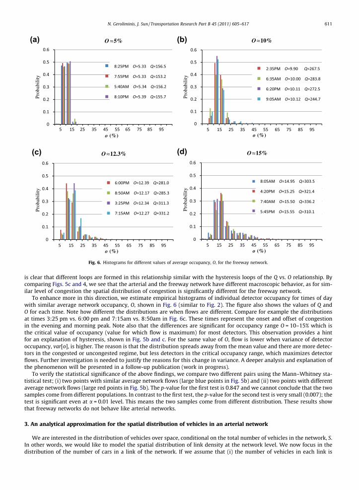
Fig. 6. Histograms for different values of average occupancy, O, for the freeway network.

N. Geroliminis, J. Sun / Transportation Research Part B 45 (2011) 605–617 611

is clear that different loops are formed in this relationship similar with the hysteresis loops of the Q vs. O relationship. Bycomparing Figs. 5c and 4, we see that the arterial and the freeway network have different macroscopic behavior, as for sim-ilar level of congestion the spatial distribution of congestion is significantly different for the freeway network.

To enhance more in this direction, we estimate empirical histograms of individual detector occupancy for times of daywith similar average network occupancy, O, shown in Fig. 6 (similar to Fig. 2). The figure also shows the values of Q andO for each time. Note how different the distributions are when flows are different. Compare for example the distributionsat times 3:25 pm vs. 6:00 pm and 7:15am vs. 8:50am in Fig. 6c. These times represent the onset and offset of congestionin the evening and morning peak. Note also that the differences are significant for occupancy range O = 10–15% which isthe critical value of occupancy (value for which flow is maximum) for most detectors. This observation provides a hintfor an explanation of hysteresis, shown in Fig. 5b and c. For the same value of O, flow is lower when variance of detectoroccupancy, var[o], is higher. The reason is that the distribution spreads away from the mean value and there are more detec-tors in the congested or uncongested regime, but less detectors in the critical occupancy range, which maximizes detectorflows. Further investigation is needed to justify the reasons for this change in variance. A deeper analysis and explanation ofthe phenomenon will be presented in a follow-up publication (work in progress).

To verify the statistical significance of the above findings, we compare two different pairs using the Mann–Whitney sta-tistical test; (i) two points with similar average network flows (large blue points in Fig. 5b) and (ii) two points with differentaverage network flows (large red points in Fig. 5b). The p-value for the first test is 0.847 and we cannot conclude that the twosamples come from different populations. In contrast to the first test, the p-value for the second test is very small (0.007); thetest is significant even at a = 0.01 level. This means the two samples come from different distribution. These results showthat freeway networks do not behave like arterial networks.

3. An analytical approximation for the spatial distribution of vehicles in an arterial network

We are interested in the distribution of vehicles over space, conditional on the total number of vehicles in the network, S.In other words, we would like to model the spatial distribution of link density at the network level. We now focus in thedistribution of the number of cars in a link of the network. If we assume that (i) the number of vehicles in each link is

612 N. Geroliminis, J. Sun / Transportation Research Part B 45 (2011) 605–617

uncorrelated with the number in all other links over the network and (ii) the probability that a randomly selected cell in thenetwork contains a car is the same, then the number of vehicles in each link should follow a binomial distribution withparameter p. Parameter p should be equal to S/NL, where NL is the total number of network cells NL = kjam � l � L, and L isthe total number of links.3 We use the average occupancy as the success probability of the binomial parameter to test ouroccupancy distribution from the experiment.

In general, if the random variable X follows the binomial distribution with parameters N and p, we define X � B(N, p). Theprobability of getting exactly x successes in N trials is given by the probability mass function.

3 Theconverg

PrðX ¼ xÞ ¼ Bðx; N; pÞ ¼N

x

� �pxð1� pÞN�x ð1Þ

The number of trials for this experiment was estimated as the maximum number of vehicles that fit in one link, N = l � kjam.As explained before, this leads to N = 22vhs and the probability of success equals to the average network occupancy, p = O. Itis found out that none of the histograms in Fig. 3 follows a binomial distribution by applying a Chi-square test. This may bedue to correlation between adjacent links, as when a downstream link becomes congested, the density of corresponding up-stream links might be affected.

Further analysis of more data from the Yokohama experiment shows that the spatial distribution of occupancy does notfollow a binomial distribution, as the spatial variance of occupancy is much higher than the one of a Binomial distributionwith probability of success equal to the average occupancy, p = O. Fig. 4 shows the variance of individual detector occupancyas average network occupancy, O, changes for a whole day. The figure contains an estimation using real data for December14, 2001 in downtown Yokohama and the estimated variance if a binomial distribution is assumed with p = O. Note the sig-nificant difference, especially as the level of congestion increases (variance 4–5 times higher).

In an arterial network, it is quite reasonable to assume that the immediate upstream link can be affected by a downstreamlink. Mathematically speaking, we assume that the probability of having a car in the cell of one link is correlated with thenumber of vehicles of its downstream link. Furthermore, in case there are some strong turning movements or ending pointlike parking ramps, the two links may be uncorrelated and the probability is equal to the a priori probability S/NL. We pres-ent here a model to estimate the spatial distribution of car density by introducing the necessary notation.

As mentioned above, the main reason of this difference with the binomial assumption is that traffic congestion in a linkhas some correlation with successive links, while a binomial distribution assumes zero correlation from one link to another.To capture this type of spatial correlation and congestion propagation from one link to another we introduce a probabilitymixture model.

Consider K + 1 successive links in an arterial network and Xk is a random variable denoting the number of vehicles in linkk = 0, 1, . . . , K (zero represents the most upstream link and K the most downstream). Then, it is assumed that Xk follows abinomial distribution with probability of success pk ¼ xk�1

N , where xk�1 is the number of vehicles in link k � 1

PrðXk ¼ xkjXk�1 ¼ xk�1Þ ¼ B xk; N;xk�1

N

� �: ð2Þ

Using the law of total expectation for the unconditional probability Pr(Xk = xk) we get

PrðXk ¼ xkÞ ¼XN

i¼0

B xk�1; N;iN

� �� Prðxk�1 ¼ iÞ: ð3Þ

Eq. (3) provides the probability density function (pdf) of Xk if X0 is known. It is not difficult to prove (tedious, but straight-forward) that the limit pdf of Xk as k ?1 if X0 � B(N, p), is taking values 0 or N with

limk!1

PrðXk ¼ NÞ ¼ p and limk!1

PrðXk ¼ 0Þ ¼ 1� p: ð4Þ

Fig. 7 shows the probability density function of Xk for k = 1, 2, . . . , 10 for p ¼ 722.

Given that an arterial network is two-dimensional, each link has more than one successive links and receives flow usuallyfrom 1 to 3 links depending on the topology of the network. To define which is the kth link in the network one can use atrajectory that travels and visits all links in the network only once. There are many different ways to do this, i.e. moving ran-domly or moving first north to south and then east to west, etc. Because of different turning percentages in each link there issome probability that correlation between link k and k � 1 is much smaller than the one described by the model in Eq. (3).For this reason we add one more parameter to the model; this is probability p, that links k and k � 1 are independent andPrðXk ¼ xkjXk�1 ¼ xk�1Þ ¼ PrðXk ¼ xkÞ ¼ Bðxk; N;OÞ.

One should expect that probability p should be higher for uncongested conditions (less spatial correlation), as trip gen-eration or turning movements can significantly affect the number of vehicles in low density links. In congested networks, oneexpects that the aforementioned effects are less intense, as links contain a large number of vehicles. Real data can provideadditional insights in this direction and p values can be estimated based on observation.Nhe Yokohama data do not allow toperform this investigation because (as explained in Geroliminis and Daganzo (2008)) the loop detector locations are not

exact distribution is hypergeometric, as if each vehicle randomly chooses without replacement an available position on the network. Hypergeometrices to binomial for high numbers of vehicles and links.

Pr

(Xk

=x k

)

xk

Fig. 7. Probability density function of the proposed model derived from Eqs. (1)–(3) for p = 7/22.

N. Geroliminis, J. Sun / Transportation Research Part B 45 (2011) 605–617 613

assigned to a digital map and there is no information which detectors are close to each other. For this reason, a statisticalestimation of p value will be performed here.

To estimate now the spatial distribution of cars in the network we need to know what is the probability that a specific linkis of type Xk, i.e. is correlated with k � 1 upstream links. This is not difficult to estimate given the modification describedabove. For a specific link in the network there is probability 1 � p that this link is correlated with the previous one and prob-ability p that it is of type X0. Thus, the type of link follows a geometric distribution with probability of success 1 � p, i.e. thenumber of failures until the first success.

PrðXk ¼ XiÞ ¼ ð1� pÞip: ð5Þ

Thus, using a mixture of Eqs. (3) and (5) we can estimate which is the spatial probability density function of linkoccupancy.

Fig. 8 compares the proposed analytical model (T) with the empirical data from Yokohama (E) and the binomial distribu-tion (B) for different values of average occupancy, O = 0.09, 0.18, 0.27, 0.32, 0.37 and 0.46, which is approximately equal withO ¼ 2

22 ;4

22 ;6

22, 722 ;

822 and 10

22, respectively. Parameter p has been calibrated to maximize goodness of fit (minimum averagesquare error).

Table 2 summarizes the results of the analysis. It also contains the average speed in the network, �v , to illustrate the levelof congestion. Note that the theoretical model developed here provides a much better fit than the binomial distribution and agood estimator of spatial variance of link occupancy, especially when the network becomes congested. Table 2b contains theresults of the statistical analysis to compare the empirical distribution vs. the proposed model (T) and the binomial distri-bution. Two commonly used tests were performed to identify, if the proposed model and the empirical data are drawn fromthe same distribution: (i) a Chi-square test (as in Section 2) and (ii) a Smirnoff–Kolmogorov test. This test estimates the max-imum vertical distance between the under consideration cumulative distribution functions, D, and compares it with athreshold value, Dcr, which depends on the number of data points and a level of significance, a. Both tests conclude thatthe proposed model (T) is not significantly different than the empirical data, while the binomial model is rejected. Valuesfor D, Dcr of the Smirnoff–Kolmogorov test and p-value of the Chi-square test are summarized in Table 2b.

4. Analysis of errors for a macroscopic fundamental diagram

This section provides an approximate estimation of the variance of the macroscopic fundamental diagram in terms ofQ(O), where O is the average occupancy of all M detectors in the network during time interval t (comparable in size withone signal cycle), and Q is the average flow of all detectors during the same time interval (interval t is omitted from the nota-tion for simplicity purposes). Variables Q and O in our analysis are unweighted averages. If we follow Edie’s definition, theapproach should be similar with the one we present here, but much more tedious.

Let us repeat the notation of a previous section; qd and od is the flow and occupancy of an individual detector d during atime interval. The relationship between qd and od (expressed as fundamental diagram) exhibits high scatter, especially for

Pro

bP

rob

Pro

b

Pro

bP

rob

Pro

b

x

o=9%

π=0.5

av. errorT-E =1.1%B-E=1.6%

x

o=18%

π=0.4

av. errorT-E =1.0%B-E=1.9%

x

x

o=27%

π=0.19

av. errorT-E =1.1%B-E=3.2%

x

x

o=32%

π=0.15

av. errorT-E =0.9%B-E=3.4%

o=37%

π=0.15

av. errorT-E =0.8%B-E=3.4%

o=46%

π=0.20

av. errorT-E =0.8%B-E=2.7%

Fig. 8. Distribution comparison between empirical data, proposed model and binomial distribution for different values of average network occupancy, O.

614 N. Geroliminis, J. Sun / Transportation Research Part B 45 (2011) 605–617

congested conditions. If qd(o) represents an average (or best fit) fundamental diagram for the individual detector we canwrite qd = qd(od) + ed(od), where ed(od) is an error, which depends on occupancy od according to the analysis for real data. Ifwe now look at all individual detectors by omitting their label d (without any type of spatial aggregation or averaging)we may fit a fundamental diagram for all individual detectors q = q(o) + e(o). Denote p(o) the continuous probability densityfunction, which shows what fraction of detectors has occupancy o and we can write:

QðOÞ ffiZ 100%

0pðoÞ � qðoÞdo ffi

XN

i¼0

~pðoiÞ � ~qðoiÞ; ð6Þ

where ~pðoiÞ is the discrete version of the continuous probability density function p(o) and ~qðoiÞ is the average flow of alldetectors in occupancy group i, i = 0, 1, . . . , N.

We now investigate the variance of Q(O). Note that this error/variance can be high (even higher than the individual detec-tor errors) if there is some type of significant correlation (not random errors) between some of the aforementioned variables.For example (i) if individual detectors exhibit significantly different individual fundamental diagrams qd(o) in different partsof the network or (ii) if congestion level is not homogeneously distributed among the network for different times of day withsimilar average occupancy O or (iii) if qd(o) is not well defined and exhibits hysteresis phenomena (like in freeways).

Table 2Analytical approximation of spatial distribution of occupancy (a) summary of results of the proposed model (T), the empirical data (E) and binomial distribution(B) and (b) statistical analysis for T vs. E and B vs. E (average error, Chi-square and Smirnoff–Kolmogorov test).

O �v (km/h) Variance p

B T E

0.09 24 1.82 6.24 8.47 0.500.18 19 3.29 18.16 20.58 0.400.27 13 4.36 23.61 22.06 0.190.32 11 4.77 25.32 24.33 0.150.37 9 5.32 24.07 23.26 0.160.46 6 5.50 20.84 18.35 0.20

�O X2 test (p-value) S-K (D value) Dcr = 8.6%(a = 0.05) (%)

Average error (%)

B–E T–E B–E T–E B–E T–E

0.09 0 0.698 9.7 7.1 1.6 1.10.18 0 0.403 17.5 7.1 1.9 1.00.27 0 0.330 19.7 6.2 3.2 1.10.32 0 0.642 21.9 5.6 3.4 0.90.37 0 0.493 26.2 4.2 3.4 0.90.46 0 0.474 15.9 4.5 2.4 1.0

N. Geroliminis, J. Sun / Transportation Research Part B 45 (2011) 605–617 615

Denote V[�] the variance of a random variable. Let ~pðoiÞ and ~qðoiÞ have random errors e~pðoiÞ and e~qðoiÞ respectively, whichare independent of each other. If the random errors of their product is independent of all other products for different i’s, thenthe variance of average network flow for a given average network occupancy O, Q(O), is

V ½QðOÞ� ffiXN

i¼0

V ½~pðoiÞ � ~qðoiÞ�: ð7Þ

The estimation of the variance of the product of two random variables is not an easy task in statistical analysis. But, ifthese two variables are independent, the variance has a closed form expression (Goodman, 1960),

V ½XY� ¼ E2½X� � V ½Y� þ E2½Y� � V ½X� þ V ½X� � V ½Y �: ð8Þ

For physical reasons, there seems no dependence between variables ~pðoiÞ and ~qðoiÞ. One variable expresses the fraction oflinks/detectors with occupancy close to oi while the other describes the average flow of the same group of links/detectors.For simplicity, we use �pi for E½~pðoiÞ� and �qi for E½~qðoiÞ�. Combining Eqs. (7) and (8) we get

V ½QðOÞ� ffiXN

i¼0

�p2i V ½e~qðoiÞ� þ �q2

i V ½e~pðoiÞ� þ V ½e~pðoiÞ�V ½e~qðoiÞ�: ð9Þ

Also, if eq(oi) is the random error of the flow for all detectors for occupancy group i (close to oi), using the central limittheorem, a good approximation for the variance of their average ~qðoiÞ is V ½eqðoiÞ� ffi V ½eqðoiÞ�

M�pi(this is the average of approxi-

mately M�pi detectors). After some manipulations Eq. (9) becomes

V ½QðOÞ� ffiXN

i¼0

1M

V ½eqðoiÞ� �pi þV ½e~pðoiÞ�

�pi

� �þ �q2

i V ½epðoiÞ�: ð10Þ

We now apply Eqs. (6)–(10) to estimate the variance of the macroscopic fundamental diagram for the site of Yokohama.Although some of the assumptions of this section may not be met in the real network, the application still illustrates how themethod may work in a real-world application, where the input data include some error.

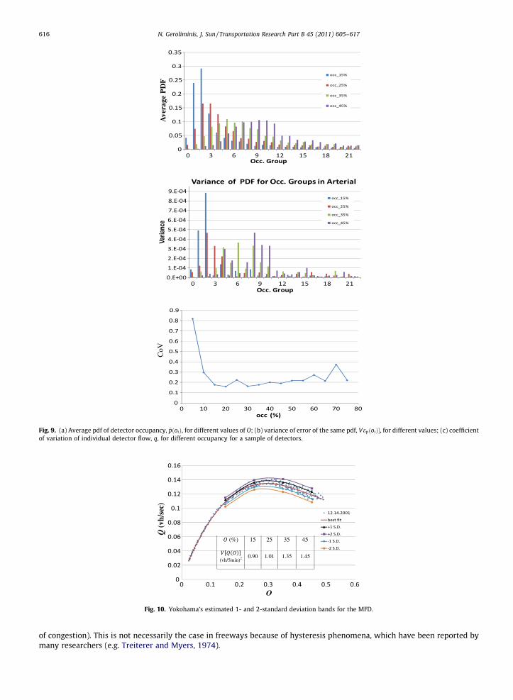
Firstly, Fig. 9a and b summarizes the estimated mean and variance of ~pðoiÞ for different occupancy groups oi for i = 0, . . . , Nfor network average occupancy o = 15%, 25%, 35% and 45%. Note that the variance of the probability density function V ½e~pðoiÞ�,is maximum for the occupancy group which is very close to the mode (the most frequent value) of ~pðoiÞ; for example group#6 for O = 35%.

Secondly, Fig. 9c shows the coefficient of variation, CoV, (dimensionless quantity: standard deviation divided by themean) of individual detector flow for different values of occupancies. Note that the CoV is almost constant at the value of0.2, for o > 5%. This is an interesting finding because by assuming that flow’s CoV is constant, one can derive a relationshipbetween the level of spatial heterogeneity (as this expressed by the variance and mean of ~pðoiÞ) and the variance of an MFD.This relationship can provide useful hints about the type of cities that exhibit a well-defined MFD. We did not categorize theCoV for different network occupancy O levels, as we do not expect that this complication could improve the estimation andhas no physical explanation (individual links are expected to produce similar q vs. o pairs independent of the aggregated level

Ave

rage

PD

FC

oV

Fig. 9. (a) Average pdf of detector occupancy, ~pðoiÞ, for different values of O; (b) variance of error of the same pdf, Ve~pðoiÞ�, for different values; (c) coefficientof variation of individual detector flow, q, for different occupancy for a sample of detectors.

Q(v

h/se

c)

O

(%) 15 25 35 45

(vh/5min)2 0.90 1.01 1.35 1.45

Fig. 10. Yokohama’s estimated 1- and 2-standard deviation bands for the MFD.

616 N. Geroliminis, J. Sun / Transportation Research Part B 45 (2011) 605–617

of congestion). This is not necessarily the case in freeways because of hysteresis phenomena, which have been reported bymany researchers (e.g. Treiterer and Myers, 1974).

N. Geroliminis, J. Sun / Transportation Research Part B 45 (2011) 605–617 617

Fig. 10 shows the results of variance estimation for Yokohama. Individual dots are Q vs. O points for every 5 min for theweekday of December 14, 2001. The lines show the 1- and 2-standard deviation bands arising from Eq. (10) on each side of afitted curve. Fig. 10 also summarizes the estimated variance. Our simplified theoretical approach describes well the varianceincrease as the level of congestion increases. Note that the CoV of the MFD is about 3–4%. This value is 5–6 times smaller thanthe CoV of an individual link, but much higher than it would have been estimated if the central limit theorem was applied forM = 500 detectors.

5. Discussion

We have studied how the spatial variability of vehicle density can affect the shape, the scatter and the existence of a well-defined macroscopic fundamental diagram. Most studies until now have looked at macroscopic relationships between theaverage flow and density, but did not explore the effect of inhomogeneous distribution of vehicles in space and time. Theresults of this paper show a sufficient condition for the existence of an MFD with low scatter. This condition states that ifthe spatial distribution of link density is the same for two different time intervals with the same number of vehicles inthe network, then these two time intervals should have the same average flows. While MFDs should be expected for arterialnetworks that satisfy the above condition, freeway networks have topological or control characteristics that are different(non-redundant, no traffic signals, hysteresis phenomena) and may not be well defined as we showed for the Twin Citiesfreeway network. Work in progress further analyses freeway data and investigates the main reasons of high scatter in Aggre-gated Traffic Relationships.

In Section 3 of the paper we derived an analytical approximation of the spatial distribution of vehicles in the network,which considered correlation between adjacent links by using a probability mixture model. We also showed that the vari-ability of vehicles in an arterial network is much higher than the one assuming a random distribution of vehicles. In Section 4we defined upper bounds for the errors of an MFD based on the errors of individual link FDs and errors in the probabilitydensity function of link occupancy.

While the results of this paper provide a clearer understanding of macroscopic modeling of traffic in cities, additional re-search is needed in different types of networks to understand how variations in the topology/structure of the network canaffect the shape and scatter of an ATR or MFD. A proper parameterization and description of heterogeneity that would yieldgood estimates of macroscopic representation of the network is of critical importance. Several questions related to this issueshould be addressed: (a) How a heterogeneous urban network can be partitioned in neighborhoods with well-defined MFDs?(b) Should this partitioning be time-dependent? (c) How are the traffic dynamics of multi-partition systems? (d) How can wecontrol inter-transfers between successive neighborhoods to increase cities’ mobility and accessibility measures? and (e)how to allocate/locate available sensing resources between different types of sensors (fixed, mobile, etc.) to maximize sys-tem observability at the city level?

Acknowledgements

The authors are grateful to Prof. Masao Kuwahara (University of Tokyo) for his continued support with the Yokohamadata and for his many comments.

References

Ardekani, S., Herman, R., 1987. Urban network-wide traffic variables and their relations. Transportation Science 21 (1), 1–16.Buisson, C., Ladier, C., 2009. Exploring the impact of the homogeneity of traffic measurements on the existence of macroscopic fundamental diagrams.

Transportation Research Record 2124, 127–136.Daganzo, C.F., 2007. Urban gridlock: macroscopic modeling and mitigation approaches. Transportation Research Part B 41 (1), 49–62.Daganzo, C.F., Geroliminis, N., 2008. An analytical approximation for the macroscopic fundamental diagram of urban traffic. Transportation Research Part B

42 (9), 771–781.Daganzo, C.F., Gayah, V., Gonzales, E., 2011. Macroscopic relations of urban traffic variables: bifurcations, multivaluedness and instability. Transportation

Research Part B 41 (1), 278–288.Edie, L.C., 1963. Discussion of traffic stream measurements and definitions. In: Almond, J. (Ed.), Proceedings of the 2nd International Symposium on the

Theory of Traffic Flow. OECD, Paris, France, pp. 139–154.Geroliminis, N., Daganzo, C.F., 2007. Macroscopic Modeling of Traffic in Cities. The 86th Transportation Research Board Annual Meeting. Paper No. 07-0413,

Washington, DC.Geroliminis, N., Daganzo, C.F., 2008. Existence of urban-scale macroscopic fundamental diagrams: some experimental findings. Transportation Research

Part B 42 (9), 759–770.Godfrey, J.W., 1969. The mechanism of a road network. Traffic Engineering and Control 11 (7), 323–327.Goodman, L., 1960. On the exact variance of products. Journal of the American Statistical Association 55 (292), 708–713.Helbing, D., 2009. Derivation of a fundamental diagram for urban traffic flow. The European Physical Journal B 70 (2), 229–241.Mahmassani, H.S., Peeta, S., 1993. Network performance under system optimal and user equilibrium dynamic assignments: implications for ATIS.

Transportation Research Record 1408, 83–93.Mahmassani, H., Williams, J.C., Herman, R., 1987. Performance of urban traffic networks. In: Gartner, N.H., Wilson, N.H.M. (Eds.), Proceedings of the 10th

International Symposium on Transportation and Traffic Theory. Elsevier, Amsterdam, The Netherlands.Olszewski, P., Fan, H.S., Tan, Y.W., 1995. Area-wide traffic speed-flow model for the Singapore CBD. Transportation Research Part A 29 (4), 273–281.Treiterer, J., Myers, J.A., 1974. The hysteresis phenomenon in traffic flow. In: Buckley, D.J. (Ed.), Proceedings of the 6th International Symposium on

Transportation and Traffic Theory, pp. 13–38.Williams, J.C., Mahmassani, H.S., Herman, R., 1987. Urban traffic network flow models. Transportation Research Record 1112, 78–88.