Transmission Line II and Matching A.Nassiri - USPASuspas.fnal.gov/materials/10MIT/Lecture4.pdf ·...
61
Massachusetts Institute of Technology RF Cavities and Components for Accelerators USPAS 2010 Transmission Line II and Matching A.Nassiri Lecture 3
-
Upload
trinhkhanh -
Category
Documents
-
view
222 -
download
1
Transcript of Transmission Line II and Matching A.Nassiri - USPASuspas.fnal.gov/materials/10MIT/Lecture4.pdf ·...

Massachusetts Institute of Technology RF Cavities and Components for Accelerators USPAS 2010
Transmission Line II and Matching
A.Nassiri
Lecture 3
Massachusetts Institute of Technology RF Cavities and Components for Accelerators USPAS 2010 2
Transmission Lines are “Guiding” devices for carryingelectromagnetic waves to and from antenna, etc.
Transmission Line behavior occurs when the wavelength of thewave is small relative to the length of the cable.
We have already shown that in a loss-less line (zero resistancealong conductors, infinite resistance between them), thepropagation speed is given by
where L and C are the inductance and capacitance per unit length.The characteristic (specific) impedance is given by:
[ ]smLC1
=ν
[ ]Ω=CL
Z

Massachusetts Institute of Technology RF Cavities and Components for Accelerators USPAS 2010 3
Types of Transmission Lines:
d
s
[ ]
[ ]
[ ]mF
ds
C
mHds
L
ds
Zr
2
2
2120
ln
ln
ln
πε=
πµ
=
Ωε
=
[ ]smLC µε
==ν11
D d
[ ]
[ ]
[ ]mF
dD
C
mHdD
L
dD
Zr
ln
ln
ln
πε=
πµ
=
Ωε
=
22
60
[ ]smLC µε
==ν11

Massachusetts Institute of Technology RF Cavities and Components for Accelerators USPAS 2010 4
Transmission Lines with Unmatched Termination:
ZL
X=-l X=0
Z0
( )
( )
( ) ( ) ( ) ( ) ( ) ( ) ( )
( ) ( ) ( ) ( ) ( )xjrxjitj
xjr
xji
tjxtjr
xtji
xtjr
xtji
eZ
eZ
xiexit,xi
eexv~exv~eet,x
e
e
ββ−ω
ββ−ωβ+ωβ−ω
β+ω
β−ω
ν−
ν==
ν+ν==ν+ν=ν∴
ν
ν
where :Similarly
where
: WaveReflected
: aveIncident W
Notice minus sign in reflected current component: Energy flows in opposite direction to incident wave.

Massachusetts Institute of Technology RF Cavities and Components for Accelerators USPAS 2010 5
( )( )
( )
( )
( ) ( )
ZZZZ
ZZZZZZZZ
ZZ
ZZi~
~
Zi~~
LL
ir
rLiL
rirLiL
ri
riL
ri
ri
L
+−
=Γ⇒=νν
∴
ν+=ν−ν+ν=ν−ν∴
⋅ν−νν+ν
=
ν−
ν=
ν+ν=ν=
ν
t Coefficien Reflected
0
0
and 00 Now
Transmission Lines with Unmatched Termination:

Massachusetts Institute of Technology RF Cavities and Components for Accelerators USPAS 2010 6
Transmission Lines with Unmatched Termination:
( ) ( )( ) ( )
( ) ( )( ) xjxj
xjxj
xjxji
xjxji
eeeeZ
xi~xv~xZ
eeZ
xi~eexv~
ββ−
ββ−
ββ−
ββ−
Γ−
Γ+==
Γ−ν
=
Γ+ν=
:Impedance dGeneralize
xj
L
Lxj
xj
L
Lxj
eZZZZ
e
eZZZZ
eZ
ββ−
ββ−
+−
−
+−
+=

Massachusetts Institute of Technology RF Cavities and Components for Accelerators USPAS 2010 7
Transmission Lines with Unmatched Termination:
( )( ) ( )( )( )( ) ( )( )
β−ββ−β
=
β+β+β−β−β−β+β−β
β−β−β+β+β−β+β−β
=
β+β−−β−β+β+β−+β−β+
=
xZjxZxZjxZ
Z
xjZxZxjZxZ
xjZxZxinjZxZxjZxZxjZxZ
xjZxZxinjZxZ
Z
xjxZZxjxZZxjxZZxjxZZ
Z
LL
L
LL
LL
LL
LL
LL
LL
sincossincos
sincossincossincoscos
sincossincossincoscos
sincossincossincossincos
2222
( )xjZZxjZZ
ZxZL
Lβ−β−
=tantan
( )l line of endat visible"" Impedance −Z
( )lll
β+β+
=−tantan
L
LjZZjZZ
ZZ

Massachusetts Institute of Technology RF Cavities and Components for Accelerators USPAS 2010 8
Transmission Lines with Unmatched Termination:
[ ]
242
4l so
WavelengthQuarter4l Suppose
π=
λ×
λπ
=λ
β→β
−λ→
∞=π2
and tan
( )[ ]
Ω=
λ∴
=ββ
=−=
λ
−∴ λ→
such that impedance sticcharacteri ofsection 4
a with
impedance of load a to impedance of line amatch can Welll
4
2
4l
Ls
L
s
LL
ZZZ
ZZ
ZZZ
tanjZtanjZZZlimZ

Massachusetts Institute of Technology RF Cavities and Components for Accelerators USPAS 2010 9
Transmission Lines :
Example- Suppose we want to match a 75Ω transmission line to a 37 Ω Marconi Antenna.
4λ 4
λ
Ω= 75sZ
Ω=×== 68527537 .Ls ZZZ Ω= 37LZ
The matching cane therefore be achieved using a Quarter-Wavelength section of 50 Ω Transmission Line.

Massachusetts Institute of Technology RF Cavities and Components for Accelerators USPAS 2010 10
Now consider a short circuit termination: (ZL=0)
Transmission Lines :
( )( )
Ω
β=β
=−∴X Reactance
lll tanZjZtanjZZZ
X(Ω)
lβ[Capacitive]
[Inductive]

Massachusetts Institute of Technology RF Cavities and Components for Accelerators USPAS 2010 11
Now consider an open circuit termination: (ZL=∞)
Transmission Lines :
X(Ω)
lβ[Capacitive]
[Inductive]
( ) ( )ll
l β−=β
=−∴ cottan Zj
jZZ
ZZL
L

Massachusetts Institute of Technology RF Cavities and Components for Accelerators USPAS 2010 12
standing waves result when a voltage generator of output voltage(VG = 1sinωt) and source impedance ZG drive a load impedanceZL through a transmission line having characteristic impedanceZ0, where ZG = Z0/ZL and where angular frequency ω correspondsto wavelength l (b). The values shown in Figure a result from areflection coefficient of 0.5.Here, probe A is located at a point at which peak voltagemagnitude is greatest—the peak equals the 1-V peak of thegenerator output, or incident voltage, plus the in-phase peakreflected voltage of 0.5 V, so on your oscilloscope you wouldsee a time-varying sine wave of 1.5-V peak amplitude (trace c).At point C, however, which is located one-quarter of awavelength (l/4) closer to the load, the reflected voltage is180° out of phase with the incident voltage and subtracts fromthe incident voltage, so peak magnitude is the 1-V incidentvoltage minus the 0.5-V reflected voltage, or 0.5 V, and youwould see the red trace. At intermediate points, you’ll see peakvalues between 0.5 and 1.5 V; at B (offset l/8 from the firstpeak) in c, for example, you’ll find a peak magnitude of 1 V.Note that the standing wave repeats every half wavelength (l/2)along the transmission line. The ratio of the maximum tominimum values of peak voltage amplitude measured along astanding wave is the standing wave ratio,SWR, SWR=3.
Figure 1
Massachusetts Institute of Technology RF Cavities and Components for Accelerators USPAS 2010 13
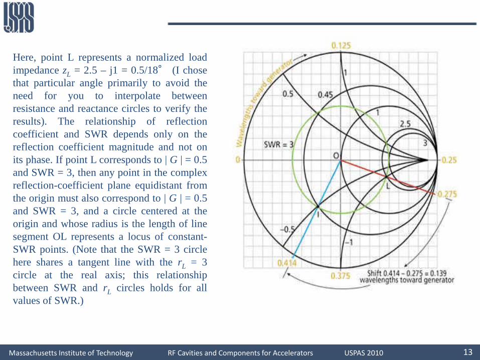
Here, point L represents a normalized loadimpedance zL = 2.5 – j1 = 0.5/18° (I chosethat particular angle primarily to avoid theneed for you to interpolate betweenresistance and reactance circles to verify theresults). The relationship of reflectioncoefficient and SWR depends only on thereflection coefficient magnitude and not onits phase. If point L corresponds to | G | = 0.5and SWR = 3, then any point in the complexreflection-coefficient plane equidistant fromthe origin must also correspond to | G | = 0.5and SWR = 3, and a circle centered at theorigin and whose radius is the length of linesegment OL represents a locus of constant-SWR points. (Note that the SWR = 3 circlehere shares a tangent line with the rL = 3circle at the real axis; this relationshipbetween SWR and rL circles holds for allvalues of SWR.)
Massachusetts Institute of Technology RF Cavities and Components for Accelerators USPAS 2010 14
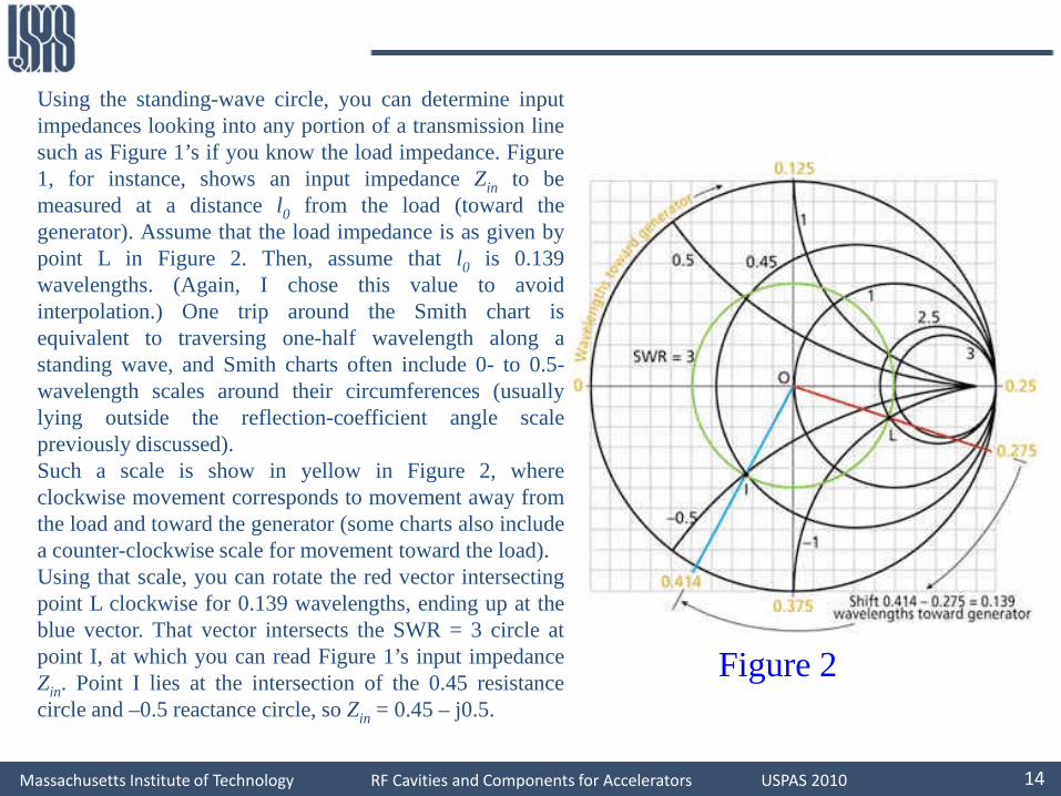
Using the standing-wave circle, you can determine inputimpedances looking into any portion of a transmission linesuch as Figure 1’s if you know the load impedance. Figure1, for instance, shows an input impedance Zin to bemeasured at a distance l0 from the load (toward thegenerator). Assume that the load impedance is as given bypoint L in Figure 2. Then, assume that l0 is 0.139wavelengths. (Again, I chose this value to avoidinterpolation.) One trip around the Smith chart isequivalent to traversing one-half wavelength along astanding wave, and Smith charts often include 0- to 0.5-wavelength scales around their circumferences (usuallylying outside the reflection-coefficient angle scalepreviously discussed).Such a scale is show in yellow in Figure 2, whereclockwise movement corresponds to movement away fromthe load and toward the generator (some charts also includea counter-clockwise scale for movement toward the load).Using that scale, you can rotate the red vector intersectingpoint L clockwise for 0.139 wavelengths, ending up at theblue vector. That vector intersects the SWR = 3 circle atpoint I, at which you can read Figure 1’s input impedanceZin. Point I lies at the intersection of the 0.45 resistancecircle and –0.5 reactance circle, so Zin = 0.45 – j0.5.
Figure 2

Massachusetts Institute of Technology RF Cavities and Components for Accelerators USPAS 2010 15
Transmission Lines Smith Chart 1
Suppose we have a load with an impedance of (40+j80)Ω which we need to match to a 100 Ω transmission line. (c 3x10⁸m/s and f=130 MHz).
( )
m.Hz
s/m.d
..
.j.jZZZ L
nL
31010130
1031350 is distance The
1350~ isgenerator therdpoint towa thisfrom ngth)(in wavele distance theChart,Smith theFrom
8040100
8040
6
8=
×
××=
λ
+=Ω
Ω+==
100 Ω ZL=40+j80 Ω
Looking in here, wesee a resistive loadof 440 Ω . We canmatch this to 100 Ωusing a 1/4λmatching section. 0.31 m

Massachusetts Institute of Technology RF Cavities and Components for Accelerators USPAS 2010 16
100 Ω ZL=40+j80 Ω
0.31 m
1/4λ
440 Ω
? Ω
MS
100 Ω
Ω=×=
=
8209440100 .
Z
ZZZ Ls
Massachusetts Institute of Technology RF Cavities and Components for Accelerators USPAS 2010 17
Smith Chart 2
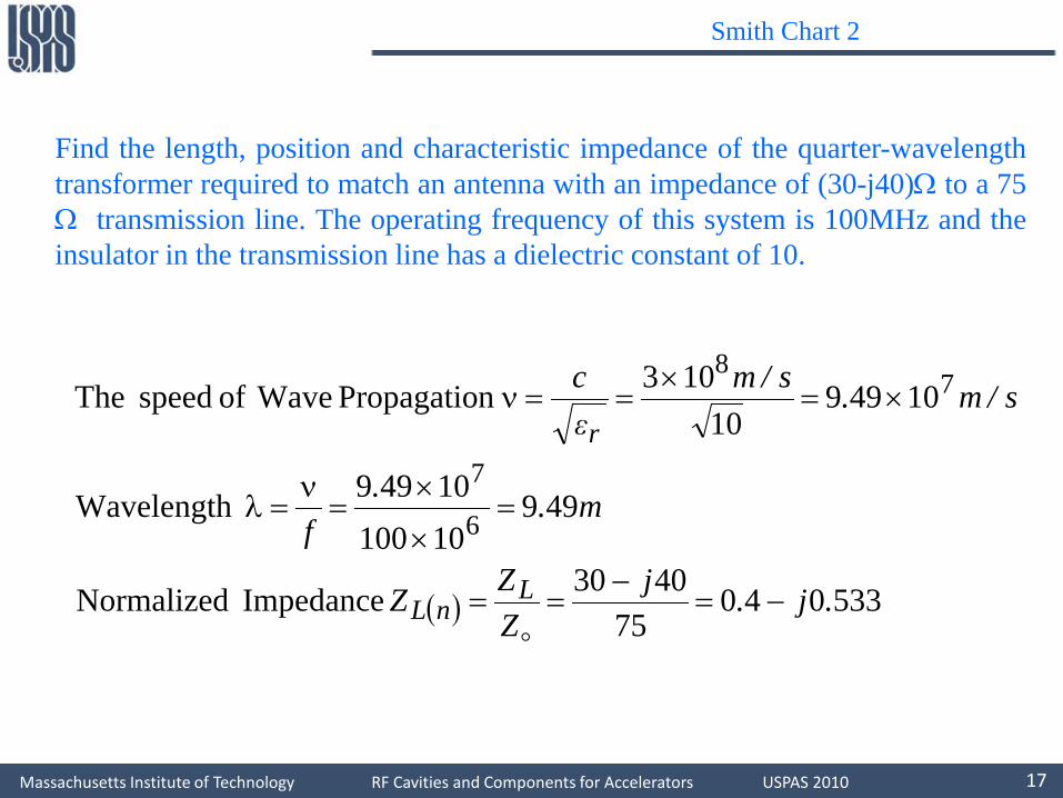
Find the length, position and characteristic impedance of the quarter-wavelengthtransformer required to match an antenna with an impedance of (30-j40)Ω to a 75Ω transmission line. The operating frequency of this system is 100MHz and theinsulator in the transmission line has a dielectric constant of 10.
( ) 53304075
4030 Impedance Normalized
4991010010499 Wavelength
1049910
103n Propagatio Waveof speed The
6
7
78
.j.jZZZ
m..f
s/m.s/mεc
LnL
r
−=−
==
=×
×=
ν=λ
×=×
==ν

Massachusetts Institute of Technology RF Cavities and Components for Accelerators USPAS 2010 18
Transmission Lines Smith Chart 2
From the Smith Chart, we find that we need to move 0.86λ away from the load (i.e., towards the generator) in order to eliminate the reactance (or imaginary) impedance component. At this point, the resistive (real) element is 0.29. Thus:
Ω=× 752175290 ..
75Ω Ω=× 3940752175 .. 75Ω 30-j40 Ω
0.25×0.949=0.237m 0.086×0.949=0.816m

Massachusetts Institute of Technology RF Cavities and Components for Accelerators USPAS 2010 19
Transmission Lines Smith Chart 3
Given that ZL=(30+j40)Ω, Z0=50 Ω, find the shortest l and ZT so that the above circuit is matched. Assume that ZT is real and loss-less.We want Zl to be real and Zin to be Z0=50 Ω in order for ZT to be real and the matching condition is satisfied. We find that ZL(n)is 0.6+j0.8. In order to make Zl(n) real, the shortest l from the Smith Chart is λ/8. Then Zl(n)=3.0, and ZL=150 Ω.Since Zin=50 Ω , we need
Ω=×== 68615050 .lZZZ inT

Massachusetts Institute of Technology RF Cavities and Components for Accelerators USPAS 2010 20
Stub Matching
We showed how a quarter-wavelength matching section can be used to impedance-match a load to a line. However, this technique has a major disadvantage: it is unlikely that one can find a transmission line with exactly the right characteristic impedance to perform the matching.
An alternative method is known as “Stub-Matching”
Using the parameters of example 1
Stub Matching requires us to convert from impedance Z to admittance Y.
Suppose we have a load with an impedance of (40+j80)Ω which we need to match to a 100 Ω transmission line. (c 3x10⁸m/s and f=130 MHz).

Massachusetts Institute of Technology RF Cavities and Components for Accelerators USPAS 2010 21
Stub Matching
( )( )
( ) 0150804080004000
8040080400
80400100
1
22 .. jj
jj
j
ZZ
YY
ZY
L
L
nLnL
−=+
−=
−−
×+
=
===
100Ω YL(n)=0.5+j1.0
Towards LoadTowards Generator

Massachusetts Institute of Technology RF Cavities and Components for Accelerators USPAS 2010 22
Stub Matching
mm 734031803210130
1036
8... =λ⇒=
××
=λ
100Ω YL(n)=0.5+j1.0
0.318 λ=0.734m
1.0+j1.65
Looking into the line at the point X, we see a normalized admittance(1+j1.65).
If we introduce a reactive admittance of –j1.65 in parallel with the line atthis point, the overall admittance will be 1.+j0 and the matching will beachieved.

Massachusetts Institute of Technology RF Cavities and Components for Accelerators USPAS 2010 23
Stub Matching
A pure reactance can be created by means of a “Stub”,i.e.,a length of transmission line with a short-circuit termination.
l
Zin yL(N)=∞
We showed before that the input impedance of a short-circuited line is given by
lβ= tanjZZ in
ll
isAdmittance Input β−=β
=∴ cottan Z
jjZ
y in1
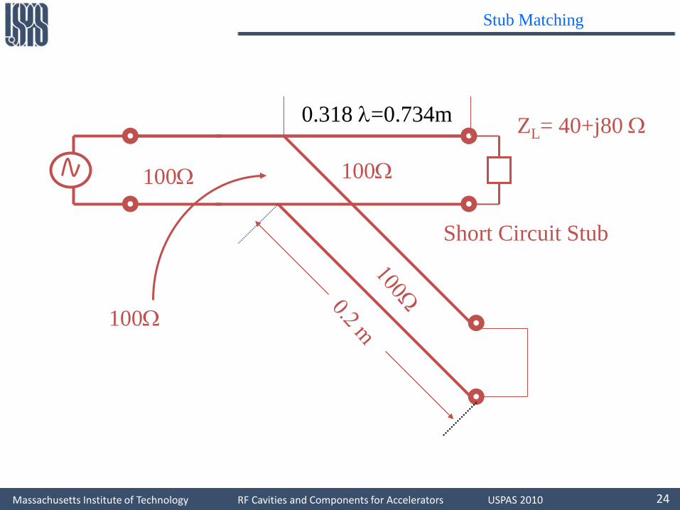
Massachusetts Institute of Technology RF Cavities and Components for Accelerators USPAS 2010 24
100Ω
ZL= 40+j80 Ω0.318 λ=0.734m
Stub Matching
100Ω
Short Circuit Stub
100Ω
Massachusetts Institute of Technology RF Cavities and Components for Accelerators USPAS 2010 25
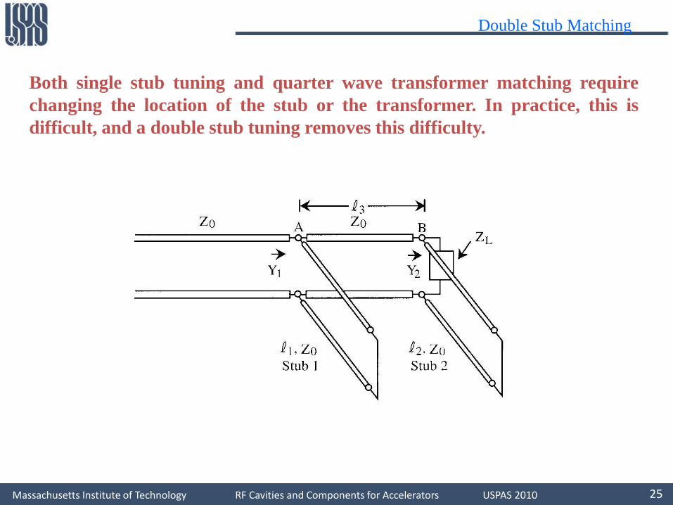
Double Stub Matching
Both single stub tuning and quarter wave transformer matching requirechanging the location of the stub or the transformer. In practice, this isdifficult, and a double stub tuning removes this difficulty.

Massachusetts Institute of Technology RF Cavities and Components for Accelerators USPAS 2010 26
Double Stub Matching:
1. In order to have a matched circuit, we should haveYl=Y0 so that Y1(n)=1. However if we change l1, thepossible values of Y1(n) trace out a circle C1.
2. If YL(n) is as shown, by changing l2, the possiblevalues of Y2(n) trace out a circle C2.
3. When l3 is added, all the possiblevalues of Y1(n)at A is transformed to B bya rotation according to the length ofl3.This constitute a circle C3 which is allthe possible values of Y2(n)obtained fromY1(n).There are only two points, P and Qthat the two circles intersect. If pick P,this correspond to the value of Y2(n).Y2n=Yln+Ystub2n.
4. The length l3. Rotates the point P to R. R has theimpedance Yn1-Ystub1n=1- Rotates the point P to R. Rhas the impedance Yn1-Ystub1n=1-Ystub1n. Ystub1n can beobtaine from SC and hence length l1.

Massachusetts Institute of Technology RF Cavities and Components for Accelerators USPAS 2010 27
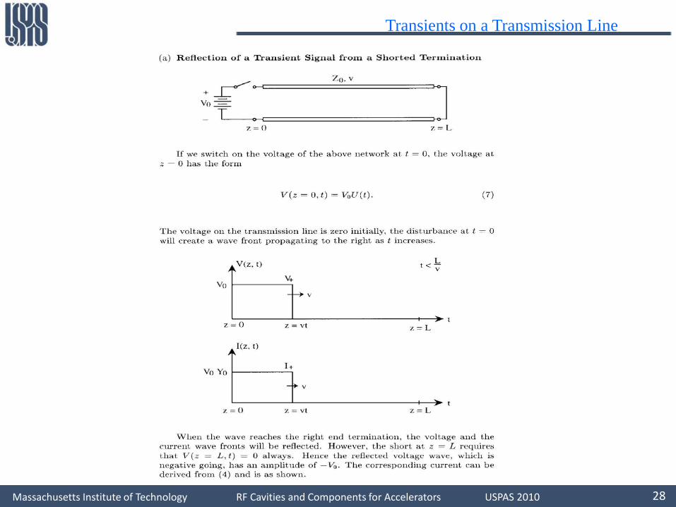
Transients on a Transmission Line
Massachusetts Institute of Technology RF Cavities and Components for Accelerators USPAS 2010 28
Transients on a Transmission Line

Massachusetts Institute of Technology RF Cavities and Components for Accelerators USPAS 2010 29
Transients on a Transmission Line

Massachusetts Institute of Technology RF Cavities and Components for Accelerators USPAS 2010 30
Transients on a Transmission Line

Massachusetts Institute of Technology RF Cavities and Components for Accelerators USPAS 2010 31
Transients on a Transmission Line

Massachusetts Institute of Technology RF Cavities and Components for Accelerators USPAS 2010 32
Smith Chart Problem 3
An inaccessible RF load is connected through a 50 Ohm loss-less T.L. to a measurement point. The line has an electrical length of 3.4 λ, and the wavelength is 0.3 m. The input impedance is Zi=110-j70Ω. Determine
a. Load impedance Z2
b. VSWR
c. Reflection coefficient at the load

Massachusetts Institute of Technology RF Cavities and Components for Accelerators USPAS 2010 33
Smith Chart Problem 3
( ) ( )
( )
( ) ( )( )
( )52
4
32
1
1
97 53012831283
is load at thet coefficien Reflection 283
5375235075047011502850402850215050
4043by load towardsP Rotate
412250
70110
P...
P.VSWRP.j..j.Z
...
.....
P.j.jZi
−∠=+−
=Γ
=Ω−=Ω−=
λ=−λ=−
λλ
−=Ω
Ω−=

Massachusetts Institute of Technology RF Cavities and Components for Accelerators USPAS 2010 34
Transmission Line
zLS
ZLSource Load
l
We assume the line is characterized by distributed resistance R, inductance L, capacitance C, and conductance G per unit length.
• •
• •v v + dv
z + dz
i + di
z
Rdz LdzCdz Gdz
i

Massachusetts Institute of Technology RF Cavities and Components for Accelerators USPAS 2010 35
Applying Kirchhoff’s voltage law to the small length dz:
ti
LdzRdzidv∂∂
+=−
ti
LRizv
∂∂
−−=∂∂
Applying Kirchhoff’s current law to the small length dz:
( ) ( ) tdvv
CdzdvvGdzdi∂+∂
++=−
tv
CGvzi
∂∂
−−=∂∂
These basic equations are difficult to solve for non-sinusoidal waves in the general case. We only consider
1) transients on lossless lines
2) sinusoidal waves on lossy lines.
Transmission Lines

Massachusetts Institute of Technology RF Cavities and Components for Accelerators USPAS 2010 36
Transmission Lines (Lossless Lines)
In a lossless line we put R-0 and G=0.
ti
Lzv
∂∂
−=∂∂
tv
Czi
∂∂
−=∂∂
If we eliminate i we obtain the one-dimensional wave equation
2
2
2
2
t
vLC
z
v
∂∂
=∂∂
The general solution contains forward and reverse traveling waves of arbitrary shape, and has the form
( ) ( ) ( )ctzVctzVtzv rf ++−=,
Exercise: Verity this solution satisfies the wave equation.

Massachusetts Institute of Technology RF Cavities and Components for Accelerators USPAS 2010 37
Transmission Lines (Lossless Lines)
V (t)
t
at z = 0 at some z > 0
z/c
V (z)
z
at some t > 0
z = ct
tv
Czi
∂∂
−=∂∂
Relation of voltage to current
Substitute v back into the equation and integrate with respect to time,
( ) ( ) ( ) ( )zfctzVctzVtziCL
rf ++−−=, f ’(z)=0 f(z)=const
( ) ( ) ( )CL
ZctzVctzVtziZ rf =+−−= 00 ,,

Massachusetts Institute of Technology RF Cavities and Components for Accelerators USPAS 2010 38
The current can be written as the sum of forward and revese components as( ) ( ) ( )ctzIctzItzi rf ++−=,
where
rrff VZ
IVZ
I00
11−==
Reflection
We consider a simple transmission line
S L
Z0 ZL
z
vL
iL At the load z =L we have
and Lrf vVVv =+=
Lrf iZVViZ 00 =−=
Lrf
rf
ZZ
VVVV
0=+−
Re-arrange to obtain at the load:0
0ZZZZ
VV
L
L
f
r
+−
=

Massachusetts Institute of Technology RF Cavities and Components for Accelerators USPAS 2010 39
Voltage reflection factor
We define the voltage reflection factor of the load as
( )0
0ZZZZ
LL
Lv +
−=Γ
Special cases
Condition ZL Γv(L)
Matched Z0 0
o/c ∞ 1
s/c 0 -1
The input resistance of the line when there is no reflected wave is
00 ZI
IZIV
iv
Rf
f
f
f
in
inin ====
The input resistance of an initially uncharged line is initially equal to the characteristic impedance.

Massachusetts Institute of Technology RF Cavities and Components for Accelerators USPAS 2010 40
Example
S L
Z0 ZL
z
vL Zs
Vsvs
is
l
At z = S( ) ( )tSVtSVv rfS ,, +=
and
( ) ( )tSVtSViZ rfS ,, −=0
vS and iS must satisfy the boundary conditions provided by the source viz.
SSSS iZVv −=
If we eliminate vs and iS from the equations above, we obtain
( ) ( )
+−
+
+
=0
0
0
0ZZZZ
tSVZZ
ZVtSV
S
Sr
SSf ,,
Vs V=Vf
Zs
Z0Vr (S, t) ≡ 0 0≤ t < 2T

Massachusetts Institute of Technology RF Cavities and Components for Accelerators USPAS 2010 41
Example
From the load end ( ) ( ) ( ) ( ) ZZZZ
LLtLVtLVS
Lvvfr +
−=ΓΓ= ,,,
ZS ZLZ0VS u(t) vL
( )tuZZ
ZV
SS
+ 0
0
( )TtuZZ
ZV
SS −
+ 0
0
( ) ( )TtuLZZ
ZV v
SS −Γ
+ 0
0
( ) ( )TtuLZZ
ZV v
SS 2
0
0 −Γ
+
( ) ( ) ( )TtuSLZZ
ZV vv
SS 2
0
0 −ΓΓ
+
( ) ( ) ( )TtuSLZZ
ZV vv
SS 3
0
0 −ΓΓ
+
( ) ( ) ( )TtuSLZZ
ZV vv
SS 32
0
0 −ΓΓ
+
( ) ( ) ( )TtuSLZZ
ZV vv
SS 42
0
0 −ΓΓ
+
( ) ( ) ( )TtuSLZZ
ZV vv
SS 422
0
0 −ΓΓ
+

Massachusetts Institute of Technology RF Cavities and Components for Accelerators USPAS 2010 42
( ) ( )[ ] ( ) ( ) ( ) ( ) ( ) ( ) ( )[ ]...+−ΓΓ+−ΓΓ+−Γ+
+
= TtuSLTtuSLTtuLZZ
ZVtv vvvvv
SSL 531 22
0
0
Example
Lattice Diagram
This has the form of a geometrical progression with common ration . For large values of t the final value of the load voltage may be shown by summing the geometrical progression above to be
( ) ( )SL vv ΓΓ
( ) ( )[ ] ( ) ( )SLL
ZZZ
Vtvvv
vS
SL ΓΓ−Γ+
+
→1
110
0
If we substitute for and in terms of ZS, ZL and Z0 and re-arrange, we get ( )LvΓ ( )SvΓ
( ) ∞→
+
→ tasZZ
ZVtv
LS
LSL

Massachusetts Institute of Technology RF Cavities and Components for Accelerators USPAS 2010 43
Example
T 3T 5T5T 7T 9Tt
vL(t)
+ LS
LS ZZ
ZV
( )[ ]LZZ
ZV v
SS Γ+
+
10
0 ( ) ( )SL vv ΓΓ Times the previous step. Could be positive or negative.
1. No activity at the load until the time T
2. The initial step at that time is the product of two factors, initially launched forward wave on the line and the sum of the unity and the reflection factor at the load known as the transmission factor at the load junction.
3. Each of the subsequent steps is a common factor times the amplitude of the preceding step.
4. The steps become progressively smaller so that the eventual load voltage converges towards a value which is recognizable as the value the load voltage would have if one simply regarded the source impedance and load impedance as forming a voltage divider delivering to the load a fraction of the source voltage.

Massachusetts Institute of Technology RF Cavities and Components for Accelerators USPAS 2010 44
Special cases
T 3T 7T5T 9T 11Tt
vL(t)
+ 0
0ZZ
ZV
SS
Waveform for a line matched at the load end.
T 3T 7T5T 9T 11Tt
vL(t)
+ L
LS ZZ
ZV
0
Waveform for a line matched at the source end.
T 3T 7T5T 9T 11Tt
vL(t)
SV2
Waveform for an open circuit line.
SV

Massachusetts Institute of Technology RF Cavities and Components for Accelerators USPAS 2010 45
Non-resistive terminations
RS
Z0VSt = 0
C
iL
vL
lS L
RS
VS
Z0( )tu
ZRZ
VVS
Sf
+=
0
0
( ) ( ) tLVtLVv rfL ,, +=
( ) ( )tLVtLViZ rfL ,, −=0
Adding these, we obtain
( )tLViZv fLL ,20 =+
2Vf
Z0 iL
vLC
for 0 ≤ t< 2T
( )TtuRZ
VZV
S
Sf −
+=
0
0

Massachusetts Institute of Technology RF Cavities and Components for Accelerators USPAS 2010 46
With ,CZ 0=τ
( ) ( )( ) teTtuVv TtSL ∀−−= τ−− 1
The reverse wave produced at the load end can then be found from
( ) ( ) ( )tLVtvtLV fLr ,, −= and is
( ) ( ) ( ) teTtuVtLV TtSr ∀
−−= τ−−
21,
To find Vr at some point z<L we add a further delay time T-t´ where t´= z/c to obtain
( ) ( ) ( ) teTttuVtzV TttSr ∀
−−′+= τ−′+− 2
212,
The total voltage on the line at any point and time is then obtained by adding to this backward wave the forward wave
( ) ( )ttuVtzV Sf ′−=21,
( ) ( ) ( ) ( )( )( )τ−′+−−−′++′−= TttS eTttuttuVtzv 2212
21,
to obtain

Massachusetts Institute of Technology RF Cavities and Components for Accelerators USPAS 2010 47
ct cTz
0<t<T
v(z)
1/2VS
1/2VS
cTz
VS
v(z)
T<t<2T
v(z)VS
cT
t >2T

Massachusetts Institute of Technology RF Cavities and Components for Accelerators USPAS 2010 48
Analysis in Frequency Domain
( ) ( ) tjezVet,zv ωℜ=
V(z) is a complex phasor representing peak value.
( ) ZIILjRdzdV
−=ω+−=
( ) YVVCjGdzdI
−=ω+−= CjGjBGYLjRjXRZ
ω+=+=ω+=+=
Solution:
Eliminating I
( )( )CjGLjRZYVdz
Vdω+ω+==γγ= 2
2
2
complex propagation constant
( ) zr
zf eVeVzV γ+γ− +=

Massachusetts Institute of Technology RF Cavities and Components for Accelerators USPAS 2010 49
Vf represents the amplitude and the phase (at the origin) of a forward wave, while Vrrepresents the amplitude and phase (both at the origin) of a reverse wave).
β+α=γ j is the complex propagation constant.
attenuation constantphase constant
The current I z) is
( ) [ ]zr
zf eVeV
ZzI γ+γ− γ+γ−−=
1
Substituting for γ
( ) [ ]zr
zf eVeV
ZY
zI γ+γ− −=
[ ]zr
zf eVeV
Zγ+γ− −=
0
1
where we introduced
CjGLjR
YZ
Zω+ω+
==0 characteristic impedance of line

Massachusetts Institute of Technology RF Cavities and Components for Accelerators USPAS 2010 50
imag
Re
γ
-γα
jβ
Argand Diagram for γ
x
jy
Z0
-Z0
Argand Diagram for Z0
fV
( ) ( ) ztjzf eeVetzV β−ωα−ℜ=,
zf eV α−
tt δ+= 0
0=t
zz
rV
zr eV α( ) ( ) ztjz
r eeVetzV β+ωαℜ=,
Forward wave on a line Reverse wave on a line

Massachusetts Institute of Technology RF Cavities and Components for Accelerators USPAS 2010 51
We define the complex voltage reflection factor Γv(z) at any point on the line as
Γv(z) = complex amplitude of the reverse voltage wave at z
complex amplitude of the forward voltage wave at z
( ) ( ) zvz
f
zr
v eeV
eVz γ
γ−
γΓ==Γ 20
When z = L, i.e. at the load, we denote Γv by Γv(L), the reflection factor of the load. When z=S, i.e. at the source, we denote Γv by Γv(S), the reflection factor looking into the line at the source end.
( )( )
( ) l
γ−−γ−
γ
γ===
ΓΓ 22
2
2ee
e
eLS SL
L
S
v
v

Massachusetts Institute of Technology RF Cavities and Components for Accelerators USPAS 2010 52
Impedance
We define impedance at any point by
( ) ( )( ) z
rz
f
zr
zf
eIeI
eVeVzIzV
zZ γ+γ−
γ+γ−
++
==
V(z) Z0,γ ZL
ZLZ(z)ZI
S z L z
Iz
( ) ( )( )zz
ZzZ
v
v
Γ−Γ+
=11
0( ) ( )
( ) 0
0ZzZZzZ
zv +−
=Γ
Combine steps to find ZI
l
l
γ−
γ−
+−
−
+−
+=
2
0
0
2
0
0
0 1
1
eZZZZ
eZZZZ
ZZ
L
L
L
L
I
llll
γ+γγ+γ
=sinhcoshsinhcosh
L
LI
ZZZZ
ZZ
0
0
0
Massachusetts Institute of Technology RF Cavities and Components for Accelerators USPAS 2010 53
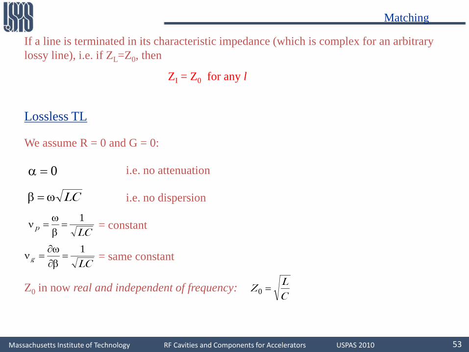
Matching
If a line is terminated in its characteristic impedance (which is complex for an arbitrary lossy line), i.e. if ZL=Z0, then
ZI = Z0 for any l
Lossless TL
We assume R = 0 and G = 0:
0=α
LCω=β
LCp1
=βω
=ν
LCg1
=β∂ω∂
=ν
i.e. no attenuation
i.e. no dispersion
= constant
= same constant
Z0 in now real and independent of frequency: CL
Z =0
Massachusetts Institute of Technology RF Cavities and Components for Accelerators USPAS 2010 54
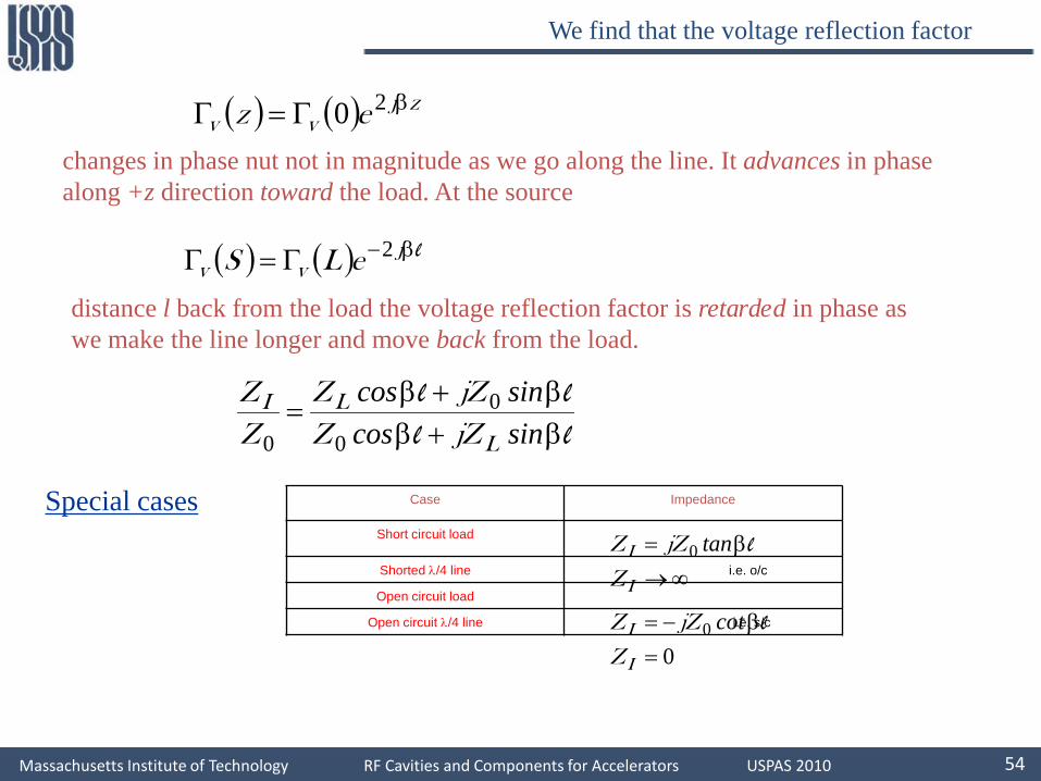
We find that the voltage reflection factor
( ) ( ) zjvv ez βΓ=Γ 20
changes in phase nut not in magnitude as we go along the line. It advances in phase along +z direction toward the load. At the source
( ) ( ) lβ−Γ=Γ jvv eLS 2
distance l back from the load the voltage reflection factor is retarded in phase as we make the line longer and move back from the load.
llll
β+ββ+β
=sincossincos
L
LI
jZZjZZ
ZZ
0
0
0
Special cases Case Impedance
Short circuit load
Shorted λ/4 line i.e. o/c
Open circuit load
Open circuit λ/4 line i.e. s/c
lβ= tan0jZZ I
∞→IZ
lβ−= cot0jZZ I
0=IZ

Massachusetts Institute of Technology RF Cavities and Components for Accelerators USPAS 2010 55
Quarter wave lines
When l = λ/4, βl = π/2. Then
LI Z
ZZ
20=
This important result means λ/4 lines can be used as transformers.
Example
λ/4
ZLZSVS
Transmission line
Z0
LI ZZZ =0 ( )( ) Ω=ΩΩ= 770501000 .Z
Normalized impedance
0ZZ
z = 11
+−
=Γzz
vv
vzΓ−Γ+
=11

Massachusetts Institute of Technology RF Cavities and Components for Accelerators USPAS 2010 56
Admittance Formulation
For every impedance Z we have a corresponding admittance Y=1/Z. It is easy to show that
llll
β+ββ+β
=sincossincos
L
LI
jYYjYY
YY
0
0
0
Special casesCase Impedance
Open circuit load
Openλ/4 line i.e. s/c
Short circuit load
Short circuit λ/4 line i.e. o/c
lβ= tan0jYYI
∞→IY
lβ−= cot0jYYI
0=IY
Quarter wave lines
LI Y
YY
20=
v
vv y
yy
YY
yΓ+Γ−
=+−
=Γ−=11
11
0
Normalized admittance

Massachusetts Institute of Technology RF Cavities and Components for Accelerators USPAS 2010 57
Current reflection factor
( ) zf
zr
ieI
eIz γ−
γ=Γ
Substituting for If and Ir in terms of Vf and Vr, we find:
vi Γ−=Γ
11
+−
=Γyy
i
i
iyΓ−Γ+
=11
Then
( ) ( ) zjii ez βΓ=Γ 20
or
( ) ( ) lβ−Γ=Γ jii eLS 2

Massachusetts Institute of Technology RF Cavities and Components for Accelerators USPAS 2010 58
Voltage Standing Wave Ratio
We look at the way the total voltage V(z) varies along the lossless line. We have, with
γ = jβ
( ) zjr
zjf eVeVzV β+β− += Vf and Vr are complex numbers
Vmax
Vmin
z
( )zV
λ/2 λ/4
rf
rf
VVV
VVV
−=
+=
min
max
rf
rf
VVVV
VV
S−+
==min
maxVSWR:
11
+−
=ΓSS
vv
vSΓ−Γ+
=
11

Massachusetts Institute of Technology RF Cavities and Components for Accelerators USPAS 2010 59
Line Parameters
Maximum and minimum values of impedance along the line can be related simply to S. When is in phase with we have a simultaneous voltage maximum and current minimum. Thus
zjf eV β− zj
reV β+
( ) 00
SZZVV
VVI
VZ
rf
rf =−
+==
min
maxmax ( ) S
ZZVV
VVIV
Zrf
rf 0
0=
+−
==max
minmin
2a 2b
πµ
=ab
L ln2
0
πε
=
ab
Cln
2
εµ
π==
ab
CL
Z ln00 2
1
and
The complex propagation constant is LCjYZj ω==β+α
There is no attenuation since we assumed there are no losses and the velocity c = ω /β is
µε==
11 LC
c

Massachusetts Institute of Technology RF Cavities and Components for Accelerators USPAS 2010 60
Consider a twin line
s
d
dsds
ds
arL >>
πµ
≈
πµ
=200 lncosh
πε
≈
πε=
ds
ds
arC
2lncoshds
ds
Z >>
εµ
π= 21 0
0 ln
Common values of Z0 are 300 Ω for communication lines, 600 Ω for telephone lines and slightly higher values are found for power lines.

Massachusetts Institute of Technology RF Cavities and Components for Accelerators USPAS 2010 61
Matching of T.L.
We recall from lumped circuit theory the maximum power transfer theorem for a.c. circuits which indicates that a sinusoidal steady state source of fixed internal voltage Vs and source impedance ZS will deliver maximum power to a load impedance ZL when ZL is adjusted to be the complex conjugate of the source impedance ZS, that is
*SL ZZ =
Matching of the T.L. at both ends makes power transfer between the source and the load take place at minimum loss, and also makes the system behavior become independent of the line length.
ZS
Z0
ZLVS
Transmission line
Matching system Matching system