Lecture 5 - USPASuspas.fnal.gov/materials/10MIT/Lecture5.pdf · Lecture 5. Massachusetts ......
65
Massachusetts Institute of Technology RF Cavities and Components for Accelerators USPAS 2010 1 Waveguides A. Nassiri Lecture 5
Transcript of Lecture 5 - USPASuspas.fnal.gov/materials/10MIT/Lecture5.pdf · Lecture 5. Massachusetts ......

Massachusetts Institute of Technology RF Cavities and Components for Accelerators USPAS 2010 1
Waveguides
A. Nassiri
Lecture 5
Massachusetts Institute of Technology RF Cavities and Components for Accelerators USPAS 2010 2
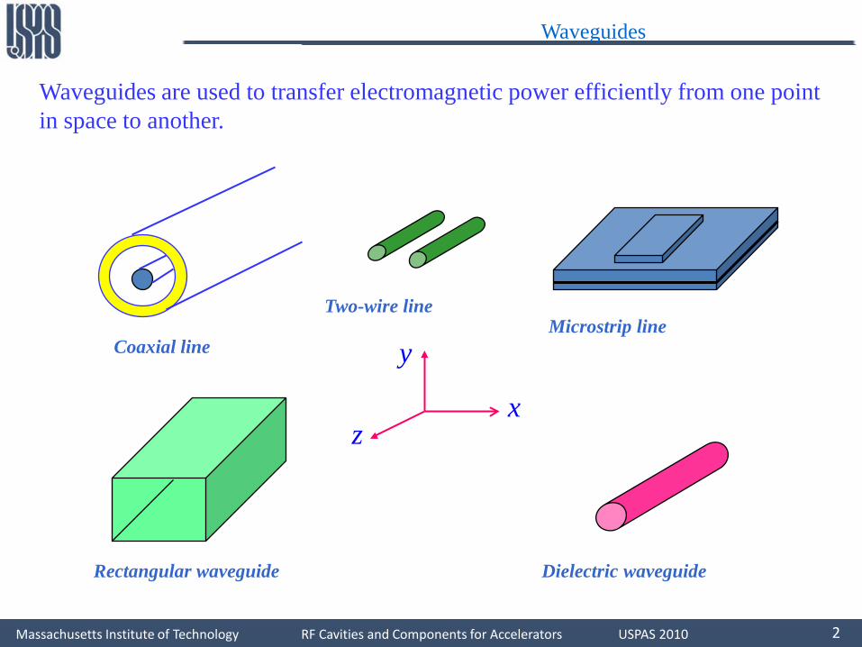
Waveguides are used to transfer electromagnetic power efficiently from one point in space to another.
Waveguides
x
y
z
Coaxial line
Two-wire lineMicrostrip line
Rectangular waveguide Dielectric waveguide
Massachusetts Institute of Technology RF Cavities and Components for Accelerators USPAS 2010 3
Waveguides
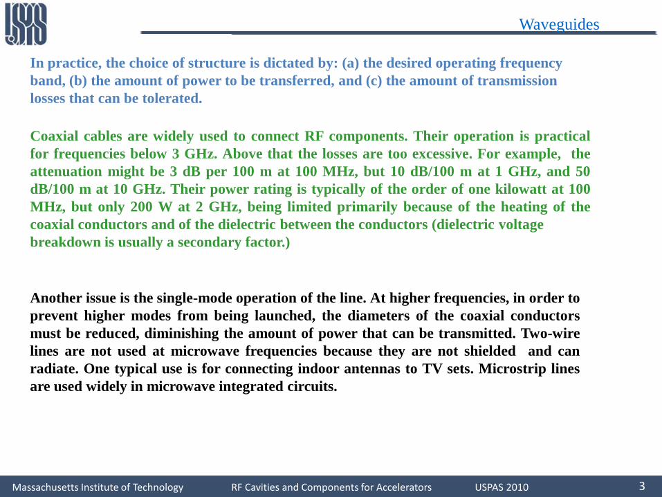
In practice, the choice of structure is dictated by: (a) the desired operating frequencyband, (b) the amount of power to be transferred, and (c) the amount of transmissionlosses that can be tolerated.
Coaxial cables are widely used to connect RF components. Their operation is practicalfor frequencies below 3 GHz. Above that the losses are too excessive. For example, theattenuation might be 3 dB per 100 m at 100 MHz, but 10 dB/100 m at 1 GHz, and 50dB/100 m at 10 GHz. Their power rating is typically of the order of one kilowatt at 100MHz, but only 200 W at 2 GHz, being limited primarily because of the heating of thecoaxial conductors and of the dielectric between the conductors (dielectric voltagebreakdown is usually a secondary factor.)
Another issue is the single-mode operation of the line. At higher frequencies, in order toprevent higher modes from being launched, the diameters of the coaxial conductorsmust be reduced, diminishing the amount of power that can be transmitted. Two-wirelines are not used at microwave frequencies because they are not shielded and canradiate. One typical use is for connecting indoor antennas to TV sets. Microstrip linesare used widely in microwave integrated circuits.
Massachusetts Institute of Technology RF Cavities and Components for Accelerators USPAS 2010 4
Waveguides
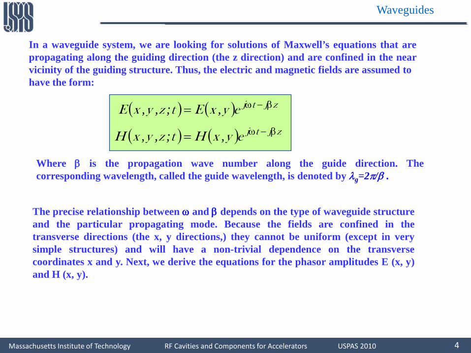
In a waveguide system, we are looking for solutions of Maxwell’s equations that arepropagating along the guiding direction (the z direction) and are confined in the nearvicinity of the guiding structure. Thus, the electric and magnetic fields are assumed tohave the form:
( ) ( ) zjtjeyxEtzyxE β−ω= ,;,,
( ) ( ) zjtjeyxHtzyxH β−ω= ,;,,
Where β is the propagation wave number along the guide direction. Thecorresponding wavelength, called the guide wavelength, is denoted by λg=2π/β .
The precise relationship between ω and β depends on the type of waveguide structureand the particular propagating mode. Because the fields are confined in thetransverse directions (the x, y directions,) they cannot be uniform (except in verysimple structures) and will have a non-trivial dependence on the transversecoordinates x and y. Next, we derive the equations for the phasor amplitudes E (x, y)and H (x, y).

Massachusetts Institute of Technology RF Cavities and Components for Accelerators USPAS 2010 5
Because of the preferential role played by the guiding direction z, it proves convenient todecompose Maxwell’s equations into components that are longitudinal, that is, along the z-direction, and components that are transverse, along the x, y directions. Thus, we decompose:
Waveguides
( ) ( ) ( ) ( ) ( ) ( )yxEzyxEyxEzyxEyyxExyxE zT
allongitudin
z
transverse
yx ,ˆ,,ˆ,ˆ,ˆ, +≡++=
In a similar fashion we may decompose the gradient operator:
zjzzyx TzTzyx ˆˆˆˆˆ β−∇=∂+∇=∂+∂+∂=∇
Where we made the replacement ∂z -jβ because of the assumed z-dependence. Introducing these decompositions into the source-free Maxwell’s equation we have:
( ) ( ) ( )( ) ( ) ( )( ) ( )( ) ( ) 00
00=+⋅β−∇=⋅∇=+⋅β−∇=⋅∇
+ωε=+×β−∇ωε=×∇+ωµ−=+×β−∇ωµ−=×∇
zTT
zTT
zTzTT
zTzTT
HzHzjH
EzEzjE
EzEjHzHzjEjH
HzHjEzEzjHjE
ˆˆˆˆ
ˆˆˆˆˆˆ

Massachusetts Institute of Technology RF Cavities and Components for Accelerators USPAS 2010 6
Transverse and Longitudinal Components
( )
( )E
Ez
EE
xy
xy
zxy
22
2
22
222
γ+∇=
∂∂
+∇=
∇+∇=∇
The wave equationsbecome now
( )( )
2 2 2
2 2 2
0
0
xy
xy
E k E
H k H
γ
γ
∇ + + =
∇ + + =
Massachusetts Institute of Technology RF Cavities and Components for Accelerators USPAS 2010 7
Solution strategy
We still have (seemingly) six simultaneous equations to solve.In fact, the 6 are NOT independent. This looks complicated!Adopt a strategy of expressing the transverse fields (the Ex,Ey,Hx,Hy components in terms of the longitudinal components Ezand Hz only. If we can do this we only need find Ez and Hz fromthe wave equations….Too easy eh!
The first step can be carried out directly from the two curlequations from the original Maxwell’s eqns. Writing these out:

Massachusetts Institute of Technology RF Cavities and Components for Accelerators USPAS 2010 8
First step
( )
( )
( )3
2
1
zxy
yz
x
xyz
Hjy
Ex
E
Hjx
EE
HjEy
E
ωµ
ωµγ
ωµγ
−=∂∂
+∂
∂
−=∂∂
−−
−=+∂∂ ( )
( )
( )6
5
4
zxy
yz
x
xyz
Ejy
Hx
H
Ejx
HH
EjHy
H
ωε
ωεγ
ωεγ
=∂∂
+∂
∂
=∂∂
−−
=+∂∂
All replaced by -γ. All fields are functions of x and y only. z∂∂

Massachusetts Institute of Technology RF Cavities and Components for Accelerators USPAS 2010 9
Result
Now, manipulate to express the transverse in terms of thelongitudinal. E.g. From (1) and (5) eliminate Ey
xz
xz Hj
xHH
jyE ωµγ
ωεγ
−=
∂∂
−−+∂∂
transverselongitudinal
222
2
where
1
kk
yEj
xH
kH
c
zz
cx
+γ=
∂∂
ωε−∂∂
γ−
=
kc is an eigenvalue(to be discussed)

Massachusetts Institute of Technology RF Cavities and Components for Accelerators USPAS 2010 10
The other components
∂∂
−∂∂−
=
∂∂
+∂∂−
=
∂∂
+∂∂−
=
∂∂
−∂∂−
=
xHj
yE
kE
yHj
xE
kE
xEj
yH
kH
yEj
xH
kH
zz
cy
zz
cx
zz
cy
zz
cx
ωµγ
ωµγ
ωεγ
ωεγ
2
2
2
2
1
1
1
1So find solutions forEz and Hz and then usethese 4 eqns to find allthe transverse components
We only need to findEz and Hz now!

Massachusetts Institute of Technology RF Cavities and Components for Accelerators USPAS 2010 11
Wave type classification
It is convenient to to classify as to whether Ez or Hz existsaccording to:
TEM: Ez = 0 Hz = 0TE: Ez = 0 Hz ≠ 0 TM Ez ≠ 0 Hz = 0
We will first see how TM wave types propagate in waveguideThen we will infer the properties of TE waves.
Massachusetts Institute of Technology RF Cavities and Components for Accelerators USPAS 2010 12
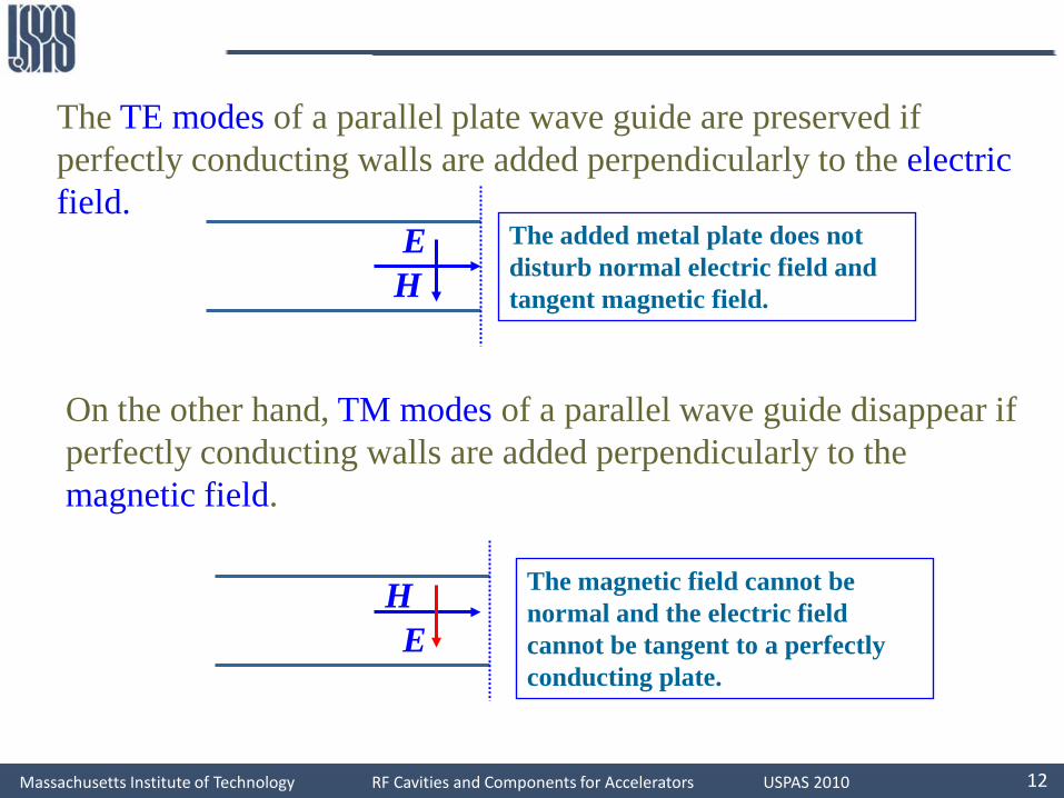
The TE modes of a parallel plate wave guide are preserved if perfectly conducting walls are added perpendicularly to the electric field.
On the other hand, TM modes of a parallel wave guide disappear if perfectly conducting walls are added perpendicularly to the magnetic field.
EH
The added metal plate does not disturb normal electric field and tangent magnetic field.
HE
The magnetic field cannot be normal and the electric field cannot be tangent to a perfectly conducting plate.

Massachusetts Institute of Technology RF Cavities and Components for Accelerators USPAS 2010 13
TM waves (Hz=0)
yE
kE
xE
kE
xE
kjH
yE
kjH
z
cy
z
cx
z
cy
z
cx
∂∂
−=
∂∂
−=
∂∂
−=
∂∂
=
2
2
2
2
γ
γ
ωε
ωε
Longitudinal: 2nd order PDE forEz. we defer solution until we havedefined a geometry plus b/c.
Transverse solutions onceEz is found
( ) 0222 =+γ+∇ zzxy EkE

Massachusetts Institute of Technology RF Cavities and Components for Accelerators USPAS 2010 14
Further Simplification
The two E-components can be combined. If we use the notation:
yy
xx
Ek
yExEE xyzxyc
yxt ˆˆ whereˆˆ 2 ∂∂
+∂∂
=∇∇−=+=γ
TM
x
y
y
xTM
zxyc
t
ZEzH
jHE
HEZ
Ek
E
×=
Ω=−==
∇−=
ˆ
2
ωεγ
γ

Massachusetts Institute of Technology RF Cavities and Components for Accelerators USPAS 2010 15
Eigenvalues
We will discover that in closed systems, solutions are possible only for discrete values of kc. There may be an infinity of values for kc, but solutions are not possible for all kc. Thus kc are known as eigenvalues. Each eigenvalue will determine theproperties of a particular TM mode. The eigenvalues will be geometry dependent.
Assume for the moment we have determined an appropriate value for kc, we now wish to determine the propagationconditions for a particular mode.

Massachusetts Institute of Technology RF Cavities and Components for Accelerators USPAS 2010 16
We have the following propagation vector components for the modes in a rectangular wave guide
2222
22222
2
22222
22
π
−
π
−µεω=β
β−β−µεω=
λπ
=
λπ
=β
π=β
π=β
β+β+β=µεω=
an
am
an
am
β
z
yxgz
z
yx
zyx
;
At the cut-off, we have
( )22
22 20
π
−
π
−µεπ==βa
na
mfcz

Massachusetts Institute of Technology RF Cavities and Components for Accelerators USPAS 2010 17
Operating bandwidth
All waveguide systems are operated in a frequency range that ensures that only the lowestmode can propagate. If several modes can propagate simultaneously, one has no controlover which modes will actually be carrying the transmitted signal. This may cause undueamounts of dispersion, distortion, and erratic operation.
A mode with cutoff frequency ωc will propagate only if its frequency is ω≥ ωc, or λ <λc. If ω< ωc, the wave will attenuate exponentially along the guide direction. Thisfollows from the ω,β relationship
2
2222222
cc c
cω−ω
=β⇒β+ω=ω
If ω≥ ωc, the wavenumber β is real-valued and the wave will propagate. But if ω< ωc,β becomes imaginary, say, β = -jα, and the wave will attenuate in the z-direction, witha penetration depth δ= 1/α:
zzj ee α−β− =

Massachusetts Institute of Technology RF Cavities and Components for Accelerators USPAS 2010 18
Operating bandwidth
If the frequency ω is greater than the cutoff frequencies of several modes, then all ofthese modes can propagate. Conversely, if ω is less than all cutoff frequencies, thennone of the modes can propagate.
If we arrange the cutoff frequencies in increasing order, ωc1< ωc2 <ωc3 < · · · , then, toensure single-mode operation, the frequency must be restricted to the interval ωc1<ω<ωc2, so that only the lowest mode will propagate. This interval defines theoperating bandwidth of the guide.
This applies to all waveguide systems, not just hollow conducting waveguides. Forexample, in coaxial cables the lowest mode is the TEM mode having no cutofffrequency, ωc1 = 0. However, TE and TM modes with non-zero cutoff frequencies doexist and place an upper limit on the usable bandwidth of the TEM mode. Similarly, inoptical fibers, the lowest mode has no cutoff, and the single-mode bandwidth isdetermined by the next cutoff frequency.

Massachusetts Institute of Technology RF Cavities and Components for Accelerators USPAS 2010 19
The cut-off frequencies for all modes are
22
22
2
21
+
=λ
+
µε=
an
am
an
am
f
c
c
With cut-off wavelengths
With indicesTE modes m=0,1,2,3,… TM modes m=1,2,3,…
n=0,1,2,3,… n=1,2,3,…
(but m=n=0 not allowed)

Massachusetts Institute of Technology RF Cavities and Components for Accelerators USPAS 2010 20
Cut-off
Since the wave propagates according to e±γz. Then propagationceases when γ = 0.
2222 implies 0 then since ccc kk ==−= µεωγµεωγ
µεπ2c
ckf =Or Cut-off
frequency

Massachusetts Institute of Technology RF Cavities and Components for Accelerators USPAS 2010 21
Write γ in terms of fc
It is usual, now to write γ in terms of the cut-off frequency.This allows us to physically interpret the result.
2
2
2
22222 1
cc
c
ccc f
fkkkk −=−=−=ωωµεωγ
This part fromthe definitionsee slide 8/5.
Substitute for µεfrom definition of fc
Recall similarityof this result withβ for an ionized gas.see slide 7/12
222 kkc −=γ

Massachusetts Institute of Technology RF Cavities and Components for Accelerators USPAS 2010 22
Conditions for Propagation
There are two possibilities here:
1cff > γ is imaginary
2
2
2
2
22
1
1
with
ffjk
kkjk
kkjj
c
c
c
−=
−=
−== βγ
We conclude that if the operational frequency is above cut-off then the wave is propagating with the form e-jβz
this is a special case of the result in the previous slide
This says now thatγ becomes jβ with
22ckk −=β
Massachusetts Institute of Technology RF Cavities and Components for Accelerators USPAS 2010 23
Different wavelengths
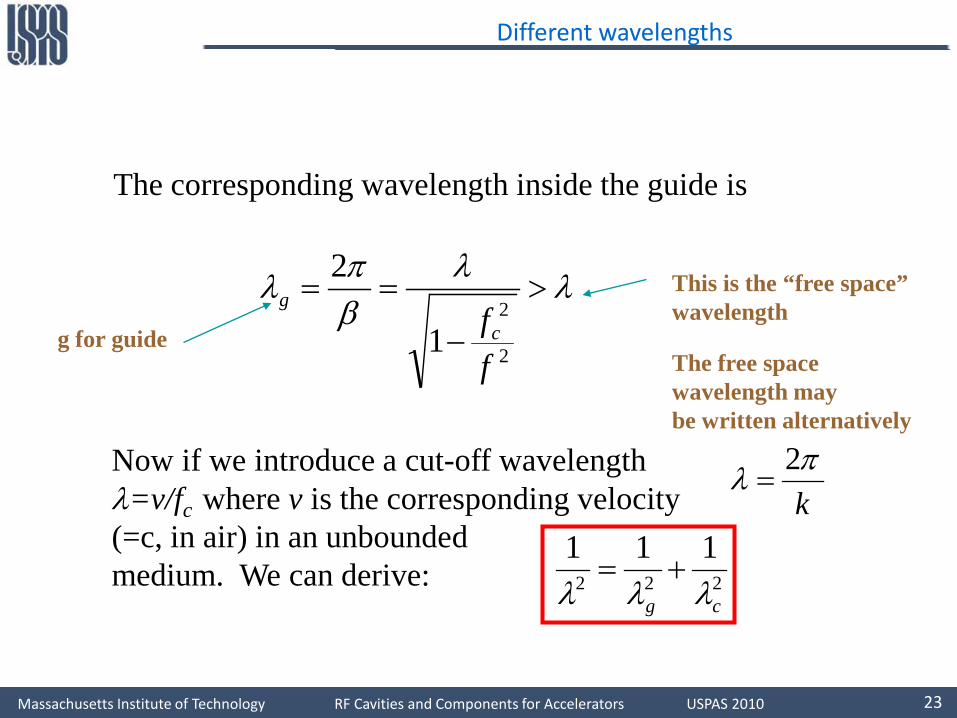
The corresponding wavelength inside the guide is
λλβπλ >
−
==
2
2
1
2
ffc
g
g for guide
This is the “free space”wavelength
The free space wavelength maybe written alternatively
kπλ 2
=Now if we introduce a cut-off wavelengthλ=v/fc where v is the corresponding velocity(=c, in air) in an unboundedmedium. We can derive: 222
111
cg λλλ+=

Massachusetts Institute of Technology RF Cavities and Components for Accelerators USPAS 2010 24
Different wavelengths
The corresponding wavelength inside the guide is
λλβπλ >
−
==
2
2
1
2
ffc
g
g for guide
This is the “free space”wavelength
The free space wavelength maybe written alternatively
kπλ 2
=Now if we introduce a cut-off wavelengthλ=v/fc where v is the corresponding velocity(=c, in air) in an unboundedmedium. We can derive: 222
111
cg λλλ+=

Massachusetts Institute of Technology RF Cavities and Components for Accelerators USPAS 2010 25
Dispersion in waveguides
The previous relationship showed that β was a function of frequency i.e. waveguides are dispersive. Hence we expect thephase velocity to also be a function of frequency. In fact:
vv
ff
vv g
c
p >=
−
==λλ
βω
2
2
1
So, as expected the phase velocity is always higher than in anunbounded medium (fast wave) and is frequency dependent.So we conclude waveguides are dispersive.
This can be > c!

Massachusetts Institute of Technology RF Cavities and Components for Accelerators USPAS 2010 26
Group velocity
This is similar to as discussed previously.
vvffvv
g
cg <=−=
∂∂
=λλ
ωβ 2
2
11
So the group velocity is always less than in an unboundedmedium. And if the medium is free space then vgvp=v2=c2
which is also as previously discussed. Finally, recall thatthe energy transport velocity is the group velocity.

Massachusetts Institute of Technology RF Cavities and Components for Accelerators USPAS 2010 27
Dispersion in waveguides
The previous relationship showed that β was a function of frequency i.e. waveguides are dispersive. Hence we expect thephase velocity to also be a function of frequency. In fact:
vv
ff
vv g
c
p >=
−
==λλ
βω
2
2
1
So, as expected the phase velocity is always higher than in anunbounded medium (fast wave) and is frequency dependent.So we conclude waveguides are dispersive.
This can be > c!
Massachusetts Institute of Technology RF Cavities and Components for Accelerators USPAS 2010 28
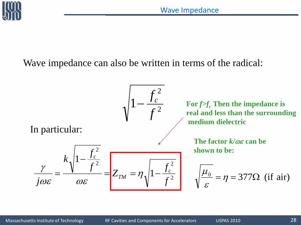
Wave Impedance
Wave impedance can also be written in terms of the radical:
2
2
1ffc−
In particular:
2
22
2
11
ffZ
ffk
jc
TM
c
−==−
= ηωεωε
γ
The factor k/ωε can be shown to be:
air) (if 3770 Ω==ηεµ
For f>fc Then the impedance is real and less than the surroundingmedium dielectric

Massachusetts Institute of Technology RF Cavities and Components for Accelerators USPAS 2010 29
Evanescent waves
2 cff < γ is real
2
2
2
2
11with ffk
kkk cc −=−==αγ
We conclude that the propagation is of the form e-αz i.e. the wave is attenuating or is evanescent as it propagates inthe +z direction. This is happening for frequencies below the cut-off frequency. At f=fc the wave is said to be cut-off.Finally, note that there is no loss mechanism contributingto the attenuation.

Massachusetts Institute of Technology RF Cavities and Components for Accelerators USPAS 2010 30
Impedance for evanescent waves
A similar derivation to that for the propagating case produces:
2
2
1c
cTM f
fkjZ −−=ωε
This says that for TM waves, the wave impedance is capacitiveand that no power flow occurs if the frequency is below cut-off. Thus evanescent waves are associated with reactive power only.

Massachusetts Institute of Technology RF Cavities and Components for Accelerators USPAS 2010 31
TE Waves
A completely parallel treatment can be made for the case ofTE propagation, Ez = 0,Hz ≠ 0. We only give the parallel results. ( )
( )HzZE
ff
jZ
Hk
H
HkH
TE
c
TE
zxyc
TEt
zzxy
×−=
−
==
∇−=
=++∇
ˆ
)(
2
2
2
222
1
0
ηγωµ
γ
γ
Massachusetts Institute of Technology RF Cavities and Components for Accelerators USPAS 2010 32
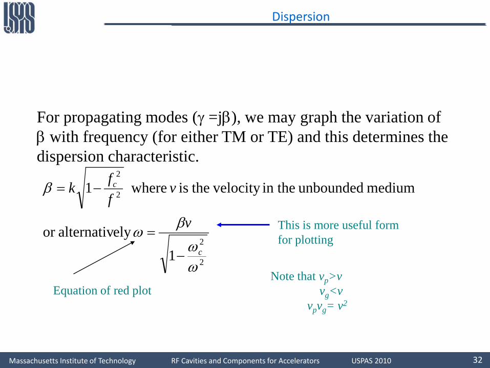
Dispersion
For propagating modes (γ =jβ), we may graph the variation of β with frequency (for either TM or TE) and this determines the dispersion characteristic.
2
2
2
2
1ely alternativor
medium unbounded in the velocity theis where1
ωω
βω
β
c
c
v
vffk
−
=
−=
This is more useful formfor plotting
Note that vp>vvg<v
vpvg= v2Equation of red plot

Massachusetts Institute of Technology RF Cavities and Components for Accelerators USPAS 2010 33
Wave Impedance
f/fcNormalized frequency
Normalizedwave impedance Z (ohms) 1
1
Evanescent here
ZTE/η
ZTM/η

Massachusetts Institute of Technology RF Cavities and Components for Accelerators USPAS 2010 34
Dispersion for Waveguide
TEMslope=ω/β
β
ω
ωc
Slope = group velocity = vg
Propagating TE and TM modes
Slope=phase velocity=vp

Massachusetts Institute of Technology RF Cavities and Components for Accelerators USPAS 2010 35
Rectangular waveguide
Convention always says that a is the long side.
X
Y
a
b ε, µ
Assume perfectly conducting walls and perfect dielectric filling the wave guide.
b
a
Massachusetts Institute of Technology RF Cavities and Components for Accelerators USPAS 2010 36
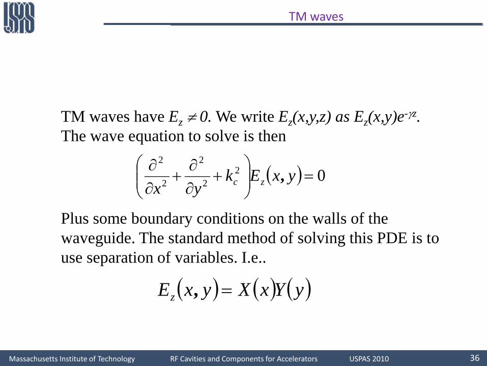
TM waves
TM waves have Ez ≠ 0. We write Ez(x,y,z) as Ez(x,y)e-γz.The wave equation to solve is then
( ) 022
2
2
2
=
+
∂∂
+∂∂ yxEk
yx zc ,
Plus some boundary conditions on the walls of the waveguide. The standard method of solving this PDE is touse separation of variables. I.e..
( ) ( ) ( )yYxXyxEz =,

Massachusetts Institute of Technology RF Cavities and Components for Accelerators USPAS 2010 37
Possible Solutions
If we substitute into the original equation we get two more equations. But this time we have full derivatives and we caneasily write solutions.
222
22
22
2
2
with
0 and 0
cyx
yx
kkk
Ykdy
YdXkdx
Xd
=+
=+=+
Mathematics tells us that the solutions depend on the sign of kx2
kx2 kx Appropriate X(x)
0 0 A0x+B0+ k A1sin kx+B1cos kx; C1ejkx +D1e-jkx
- jk A2sinh kx +B2cosh kx; C2ekx +D2e-kx

Massachusetts Institute of Technology RF Cavities and Components for Accelerators USPAS 2010 38
Boundary conditions
Boundary conditions say that the tangential components of Ezvanish on the walls of the guide :
( )( )( )( ) walls.bottom and top
0,00,E
walls.handright andleft 0,0,0
z
==
==
bxEx
yaEyE
z
z
z
We choose the sin/cos form (why?) and directly write:
( ) ( )( )ykBykAxkBxkAyxE yyxxz cossincossin, 2211 ++=

Massachusetts Institute of Technology RF Cavities and Components for Accelerators USPAS 2010 39
Final solution
Using the boundary conditions, we find:X(x) must be in the form sinkxxY(y) must be in the form sinkyy
,.....,,, 321 andinteger n m, with =
=
=nm
bnk
amk
y
x
π
π
( )22
2
0
+
=
=
bn
amk
byn
axmEyxE
c
z
ππ
ππ sinsin,
We can only get discretevalues of kc -eigenvalues!
This satisfies all theboundary conditions
Do not start from 0

Massachusetts Institute of Technology RF Cavities and Components for Accelerators USPAS 2010 40
Mode numbers (m,n)
The m,n numbers will give different solutions for Ez (as well asall the other transverse components. Each m,n combination will correspond to a mode which will satisfy all boundary and wave equations. Notice how the modes depend on the geometry (a,b)!
We usually refer to the modes as TMmn or TEmn eg TM2,3Thus each mode will specify a unique field distribution in theguide. We now have a formula for the parameter kc oncewe specify the mode numbers.
The concept of a mode is fundamental to many E/M problems.

Massachusetts Institute of Technology RF Cavities and Components for Accelerators USPAS 2010 41
From previous formulas, we have directly upon using the value kc
22
22
22
1
+
=
+
=
bn
am
bn
amf
c
c
λ
µε
Note this!

Massachusetts Institute of Technology RF Cavities and Components for Accelerators USPAS 2010 42
TE Modes
For TE modes, we have Ez = 0, Hz ≠ 0 as before.
( ) 022
2
2
2
=
+
∂∂
+∂∂ yxHk
yx zc ,
==⇒∂∂
==⇒∂∂
==⇒∂∂
==⇒∂∂
=
=
=
=
bEy
H
Ey
H
axEx
H
xEx
H
xy
z
xy
z
yx
z
yx
z
yat 0
0yat 0
at 0
0at 0
0
0
0
0
Boundaryconditions
Boundary conditionsfor Hz (longitudinal) are equivalentlyexpressed in terms ofEx and Ey (transverse)

Massachusetts Institute of Technology RF Cavities and Components for Accelerators USPAS 2010 43
TEmn Results
The expressions for fc and λc are identical to the TM case. But this time we have that the TE dominant mode (ie. the TE mode with the lowest cut-off frequency) is TE10 This mode has an even lower cut-off frequency than TM11 and is said to be the Dominant Mode for a rectangular waveguide. ( )
( )
( ) aav
af
byn
axmHyxH
TEc
TEc
z
222
1
coscos,
10
10
0
=
==
=
λµε
ππThis is providedwe label the largeside ‘a’ and associatethis side with the mode number ‘m’

Massachusetts Institute of Technology RF Cavities and Components for Accelerators USPAS 2010 44
View of TE10 mode for waveguide.
TE10
H field
E field

Massachusetts Institute of Technology RF Cavities and Components for Accelerators USPAS 2010 45
For mono-mode (or single-mode) operation, only the fundamental TE10 mode should be propagating over the frequency band of interest.
The mono-mode bandwidth depends on the cut-off frequency of the second propagating mode. We have two possible modes to consider, TE01 and TE20.
( )
( ) ( )1020
01
212
1
TEfa
TEf
bTEf
cc
c
=µε
=
µε=

Massachusetts Institute of Technology RF Cavities and Components for Accelerators USPAS 2010 46
( ) ( ) ( )µε
===⇒=a
TEfTEfTEfa
b ccc12
2 102001 If
( ) ( ) ( )2001102TEfTEfTEf
aba ccc <<⇒>> If
f
Mono-mode Bandwidth
0 fc(TE10) fc(TE20)
f
Mono-mode Bandwidth
0 fc(TE10) fc(TE20)fc(TE01)

Massachusetts Institute of Technology RF Cavities and Components for Accelerators USPAS 2010 47
( ) ( )01202TEfTEf
ab cc <⇒< If
f
Mono-mode Bandwidth
0 fc(TE10) fc(TE20)
f
Useful Bandwidth
0 fc(TE10) fc(TE20) fc(TE01)
fc(TE01)In practice , a safety margin of about 20% is considered, so that the useful bandwidth is less than the maximum mono-mode bandwidth. This is necessary to make sure that the first mode (TE10) is well above cut-off, and the second mode (TE01 or TE20) is strongly evanescent.
Safety margin

Massachusetts Institute of Technology RF Cavities and Components for Accelerators USPAS 2010 48
If a=b (square wave guide) ⇒ ( ) ( )2010 TEfTEf cc =
f0 fc(TE10) fc(TE20)fc(TE01) fc(TE02)
In the case of perfectly square wave guide, TEm0 and TE0nmodes with m=n are are degenerate with the same cut-off frequency.
Except for orthogonal field orientation, all other properties of the degenerate modes are the same.
Massachusetts Institute of Technology RF Cavities and Components for Accelerators USPAS 2010 49
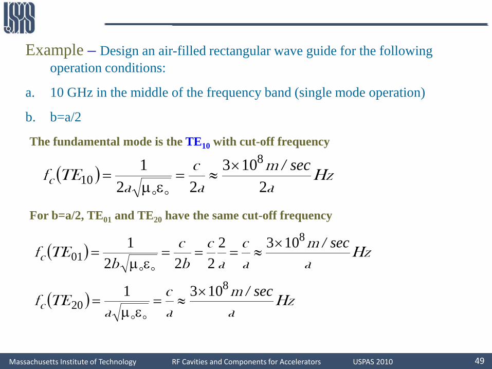
Example – Design an air-filled rectangular wave guide for the following operation conditions:
a. 10 GHz in the middle of the frequency band (single mode operation)
b. b=a/2
The fundamental mode is the TE10 with cut-off frequency
( ) Hzam
ac
aTEfc 2
10322
1 8
10sec/×
≈=εµ
=
For b=a/2, TE01 and TE20 have the same cut-off frequency
( )
( ) Hzam
ac
aTEf
Hzam
ac
ac
bc
bTEf
c
c
sec/
sec/
8
20
8
01
1031
1032222
1
×≈=
εµ=
×≈===
εµ=
Massachusetts Institute of Technology RF Cavities and Components for Accelerators USPAS 2010 50
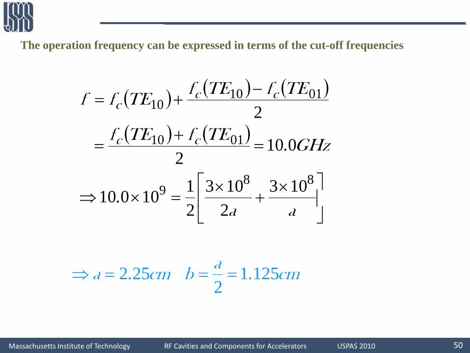
The operation frequency can be expressed in terms of the cut-off frequencies
( ) ( ) ( )
( ) ( )
×+
×=×⇒
=+
=
−+=
aa
GHzTEfTEf
TEfTEfTEff
cc
ccc
889
0110
011010
1032103
2110010
0102
2
.
.
cma
bcma 12512
252 .. ===⇒

Massachusetts Institute of Technology RF Cavities and Components for Accelerators USPAS 2010 51
An example
We consider an air filled guide, so εr=1. The internal size of the guide is 0.9 x 0.4 inches (waveguides come in standard sizes).The cut-off frequency of the dominant mode:
( )
( ) GHzkf
ak
bn
amk
cTEc
TEc
c
5662
103431372
43137
10.16mm40.b 22.86mm;90.a
8
00
22
10
10
..
.
=××
==
==
=′′==′′=
+
=
πεµπ
π
ππ

Massachusetts Institute of Technology RF Cavities and Components for Accelerators USPAS 2010 52
An example
The next few modes are:
( )( )( )
,110120,10, is mode oforder ascending the86.27421.30938.338
20
01
11
=
=
=
c
c
c
kkk
The next cuff-off frequency after TE10 will then be
( ) GHzf TEc 12132
10386274 8
20..
=××
=π
So for single mode operation we must operate the guide withinthe frequency range of 6.56<f <13.12GHz.

Massachusetts Institute of Technology RF Cavities and Components for Accelerators USPAS 2010 53
It is not good to operate too close to cut-off for the reason thatthe wall losses increases very quickly as the frequency approachescut-off. A good guideline is to operate between 1.25fc and 1.9fc.This then would restrict the single mode operation to 8.2 to 12.5GHz.
The propagation coefficient for the next higher mode is:
( ) ( ) 2
2
2022
2020
1c
cc ffkkk −=−=γ
Specify an operating frequency f, half way in the original range of TE10 i.e.. 9.84GHz.
An example

Massachusetts Institute of Technology RF Cavities and Components for Accelerators USPAS 2010 54
( )
.evanescentstrongly very is TE ie. dB/m 1581 8.7 x 181.8 dBin or 8181 So
(Real) 81811213849186274
20
2
20
==
=
−=
mNp /.
....
α
γ
In comparison for TE10:
( ) ( )
rad/m153.64 So
)(Imaginary 641535668491431371
2
210
2
1010
=
=
−=−=
β
γ jffkc
c ....
All further higher order modes will be cut-off with higher ratesof attenuation.
An example
Massachusetts Institute of Technology RF Cavities and Components for Accelerators USPAS 2010 55
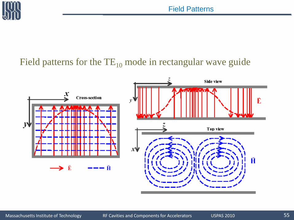
Field Patterns
Field patterns for the TE10 mode in rectangular wave guide
Massachusetts Institute of Technology RF Cavities and Components for Accelerators USPAS 2010 56
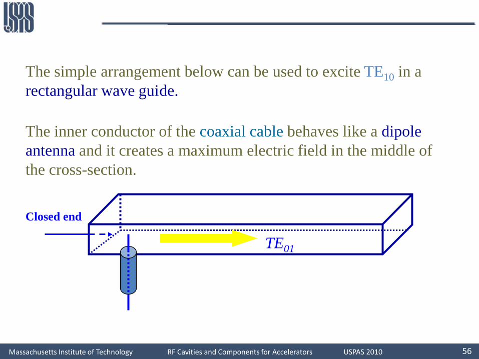
The simple arrangement below can be used to excite TE10 in a rectangular wave guide.
The inner conductor of the coaxial cable behaves like a dipole antenna and it creates a maximum electric field in the middle of the cross-section.
TE01
Closed end

Massachusetts Institute of Technology RF Cavities and Components for Accelerators USPAS 2010 57
Waveguide Cavity Resonator
The cavity resonator is obtained from a section of rectangular wave guide, closed by two additional metal plates. We assume again perfectly conducting walls and loss-less dielectric.
d
a
bdpβ
bnβ
amβ
z
y
x
π=
π=
π=
Massachusetts Institute of Technology RF Cavities and Components for Accelerators USPAS 2010 58
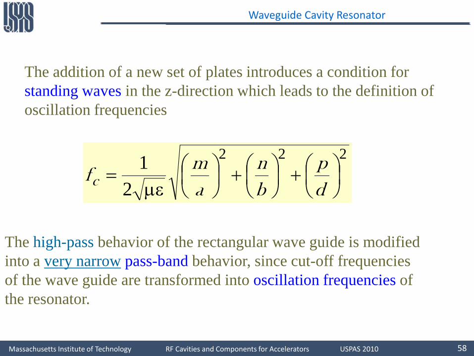
Waveguide Cavity Resonator
The addition of a new set of plates introduces a condition for standing waves in the z-direction which leads to the definition of oscillation frequencies
222
21
+
+
µε=
dp
bn
am
fc
The high-pass behavior of the rectangular wave guide is modified into a very narrow pass-band behavior, since cut-off frequencies of the wave guide are transformed into oscillation frequencies of the resonator.

Massachusetts Institute of Technology RF Cavities and Components for Accelerators USPAS 2010 59
Waveguide Cavity Resonator
In the wave guide, each mode isassociated with a band of frequencieslarger the cut-off frequency.
In the resonator, resonant modes canonly exist in correspondence of discreteresonance frequencies.
0 fc1 fc2 f fc10 fc2 f

Massachusetts Institute of Technology RF Cavities and Components for Accelerators USPAS 2010 60
Waveguide Cavity Resonator
The cavity resonator will have modes indicated as
TEmnp TMmnpThe values of the index corresponds to periodicity (number of sine orcosine waves) in three direction. Using z-direction as the reference forthe definition of transverse electric or magnetic fields, the allowedindices are
===
===
,...,,,,...,,,,...,,,
,...,,,,...,,,,...,,,
321032103210
321032103210
pnm
TMpnm
TE
With only one zero index m or n allowed
The mode with lowest resonance frequency is called dominant mode. In case a ≥ d>b the dominant mode is the TE101.

Massachusetts Institute of Technology RF Cavities and Components for Accelerators USPAS 2010 61
Waveguide Cavity Resonator
Note that a TM cavity mode, with magnetic field transverse to the z-direction, it is possible to have the third index equal zero. This is because themagnetic field is going to be parallel to the third set of plates, and it cantherefore be uniform in the third direction, with no periodicity.
The electric field components will have the following form that satisfies theboundary conditions for perfectly conducting walls.
π
π
π
= zdp
ybn
xa
mE xx sinsincosE
π
π
π
= zdp
ybn
xa
mE yy sincossinE
π
π
π
= zdp
ybn
xa
mE zy cossinsinE

Massachusetts Institute of Technology RF Cavities and Components for Accelerators USPAS 2010 62
Waveguide Cavity Resonator
The amplitudes of the electric field components also must satisfy the divergence condition which, in absence of charge is
00 =
π
+
π
+
π
⇒=⋅∇ zyx Edp
Ebn
Ea
mE
The magnetic field intensities are obtained from Ampere’s law:
π
π
π
ωµβ−β
= zdp
ybn
xa
mj
EEH zyyz
x coscossin
π
π
π
ωµβ−β
= zdp
ybn
xa
mj
EEH xzzx
y cossincos
π
π
π
ωµβ−β
= zdp
ybn
xa
mj
EEH yxxy
z sincoscos
Massachusetts Institute of Technology RF Cavities and Components for Accelerators USPAS 2010 63
Waveguide Cavity Resonator
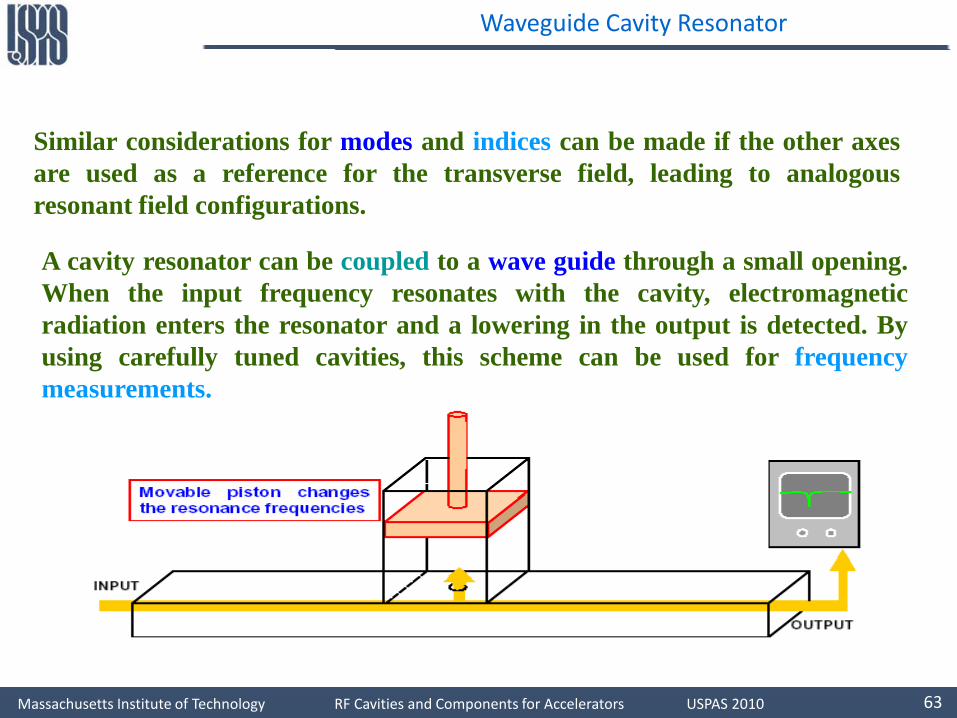
Similar considerations for modes and indices can be made if the other axesare used as a reference for the transverse field, leading to analogousresonant field configurations.
A cavity resonator can be coupled to a wave guide through a small opening.When the input frequency resonates with the cavity, electromagneticradiation enters the resonator and a lowering in the output is detected. Byusing carefully tuned cavities, this scheme can be used for frequencymeasurements.
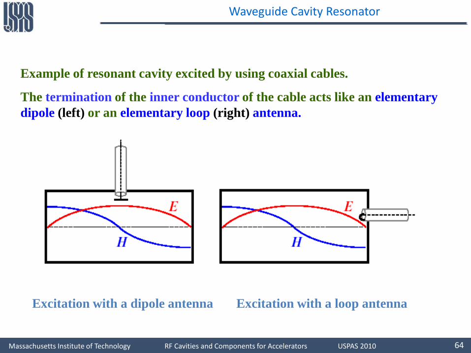
Massachusetts Institute of Technology RF Cavities and Components for Accelerators USPAS 2010 64
Waveguide Cavity Resonator
Example of resonant cavity excited by using coaxial cables.
The termination of the inner conductor of the cable acts like an elementary dipole (left) or an elementary loop (right) antenna.
Excitation with a dipole antenna Excitation with a loop antenna

Massachusetts Institute of Technology RF Cavities and Components for Accelerators USPAS 2010 65
Characteristics of some standard air-filled rectangular waveguides.
Here are some standard air-filled rectangular waveguides with their namingdesignations, inner side dimensions a, b in inches, cutoff frequencies in GHz,minimum and maximum recommended operating frequencies in GHz, powerratings, and attenuations in dB/m (the power ratings and attenuations arerepresentative over each operating band.) We have chosen one example fromeach microwave band.
Waveguides