Transient Sensitivity Analysis - TU/e · PDF fileTalk Structure Introduction Recap Sensitivity...
67
Transient Sensitivity Analysis CASA Day 13th Nov 2007 Zoran Ilievski Zoran Ilievski Transient Sensitivity Analysis
-
Upload
truongdiep -
Category
Documents
-
view
229 -
download
1
Transcript of Transient Sensitivity Analysis - TU/e · PDF fileTalk Structure Introduction Recap Sensitivity...

Transient Sensitivity AnalysisCASA Day 13th Nov 2007
Zoran Ilievski
Zoran Ilievski
Transient Sensitivity Analysis
Talk Structure
Introduction
Recap Sensitivity
Examples and Results
Further Work
Zoran Ilievski
Transient Sensitivity Analysis
Talk Structure
Introduction
Recap Sensitivity
Examples and Results
Further Work
Zoran Ilievski
Transient Sensitivity Analysis

Talk Structure
Introduction
Recap Sensitivity
Examples and Results
Further Work
Zoran Ilievski
Transient Sensitivity Analysis

Talk Structure
Introduction
Recap Sensitivity
Examples and Results
Further Work
Zoran Ilievski
Transient Sensitivity Analysis

Talk Structure
Introduction
Recap Sensitivity
Examples and Results
Further Work
Zoran Ilievski
Transient Sensitivity Analysis

Talk Structure
Introduction
Recap Sensitivity
Examples and Results
Further Work
Zoran Ilievski
Transient Sensitivity Analysis

Introduction
State Sensitivity
∆ L & ∆ W will gives ∆R
Which will change the states/voltages x(t)
Zoran Ilievski
Transient Sensitivity Analysis

Introduction
Function Sensitivity
More complex functions such as Gain are expressions based onthese states and parameters.
As parameters change, the Gain (or other functions) will alsochange.
Zoran Ilievski
Transient Sensitivity Analysis

Introduction - Circuit DAE Description
d
dt[q(x(t))] + j(x(t)) = s(t)
x(t) ∈ RN is the state vector.
j & q are current and charge densities
s(t) contains all source values.
Solve the DAE obtained from Kirchhoffs laws, to findbehaviour.
Zoran Ilievski
Transient Sensitivity Analysis
Introduction - The influence of a parameter P
d
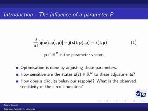
dt[q(x(t,p),p)] + j(x(t,p),p) = s(t,p) (1)
p ∈ RP is the parameter vector.
Optimisation is done by adjusting these parameters.
How sensitive are the states x(t) ∈ RN to these adjustments?
How does a circuits behaviour respond? What is the observedsensitivity of the circuit function?
Zoran Ilievski
Transient Sensitivity Analysis
Introduction - State sensitivity
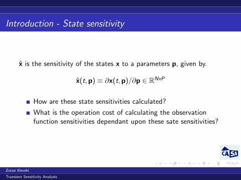
x is the sensitivity of the states x to a parameters p, given by.
x(t,p) ≡ ∂x(t,p)/∂p ∈ RNxP
How are these state sensitivities calculated?
What is the operation cost of calculating the observationfunction sensitivities dependant upon these sate sensitivities?
Zoran Ilievski
Transient Sensitivity Analysis

Introduction - Circuit Observation Functions
Gf (x(p),p) =
∫ T
0F(x(t,p),p)dt. (2)
ddp
Gf (x(p),p) =
∫ T
0
∂F
∂x· x +
∂F
∂pdt. (3)
The Gain of an amplifier circuit can be called the observationfunction of that design
You can see that the state sensitivity is central to the overallfunction sensitivity
The cost of x is the main burden.
Zoran Ilievski
Transient Sensitivity Analysis

Introduction
How are these state and observation sensitivities calculated?
Zoran Ilievski
Transient Sensitivity Analysis
Introduction
Recap Sensitivity
Examples and Results
Further Work
Zoran Ilievski
Transient Sensitivity Analysis
Recap - State sensitivity
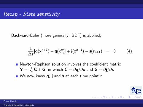
Backward-Euler (more generally: BDF) is applied:
1
∆t[q(xn+1)− q(xn)] + j(xn+1)− s(tn+1) = 0 (4)
Newton-Raphson solution involves the coefficient matrixY = 1
∆t C + G, in which C = ∂q/∂x and G = ∂j/∂x
We now know q, j and s at each time point t
Zoran Ilievski
Transient Sensitivity Analysis

Recap - State sensitivity
Differentiation w.r.t. parameter P gives:
0 =1
∆t[∂q
∂p
n+1
− ∂q
∂p
n
] +1
∆t[Cxn+1 − Cxn] + Gxn+1 +
∂j
∂p− ∂s
∂p
After slight re-arrangement:
((1/∆t)C + G)︸ ︷︷ ︸Y
xn+1 = − 1
∆t[∂q
∂p
n+1
− ∂q
∂p
n
] + (1/∆t)Cxn − ∂j
∂p+∂s
∂p︸ ︷︷ ︸f
Zoran Ilievski
Transient Sensitivity Analysis
Recap - State sensitivity - Cost
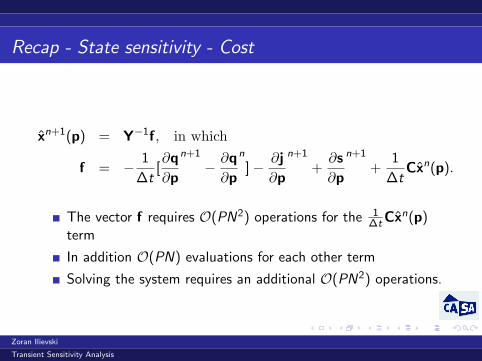
xn+1(p) = Y−1f, in which
f = − 1
∆t[∂q
∂p
n+1
− ∂q
∂p
n
]− ∂j
∂p
n+1
+∂s
∂p
n+1
+1
∆tCxn(p).
The vector f requires O(PN2) operations for the 1∆t Cxn(p)
term
In addition O(PN) evaluations for each other term
Solving the system requires an additional O(PN2) operations.
Zoran Ilievski
Transient Sensitivity Analysis

Recap - Circuit Observation Functions
We now have an analysis of x
But what part does x play in the sensitivity analysis of anyobservation function.
Gf (x(p),p) =
∫ T
0F(x(t,p),p)dt.
Zoran Ilievski
Transient Sensitivity Analysis

Recap - Circuit Observation Functions
Gf (x(p),p) =
∫ T
0F(x(t,p),p)dt.
ddp
Gf (x(p),p) =
∫ T
0
∂F
∂x· x +
∂F
∂pdt.
You can see that the state sensitivity is central to the overallfunction sensitivity.
The cost of x is the main burden.
Zoran Ilievski
Transient Sensitivity Analysis

Recap - Direct Forward Method
It is no supprise that the emphasis in sensitivity analysis is theefficient calculation of x or indeed the inner product.
∂F
∂x· x =
∂F
∂x.Y−1f = [Y−T [
∂F
∂x]T ]T f
This can be calculated in O(min(F ,P)N2 + FPN) operations.
This is for the Direct Forward Method
Circuits often contain many thousands of parameters, need abetter method.
Zoran Ilievski
Transient Sensitivity Analysis

Recap - Backward Adjoint Method
Small N Large Circuits, Large N
Direct Foward Feasible Expensive
Backward Adjoint Feasible
Elimination of x , and so reducing the complexity is done usinga backward integration technique.
An less expensive expression of the observation sensitivity interms of λ(t)
Zoran Ilievski
Transient Sensitivity Analysis
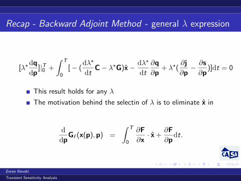
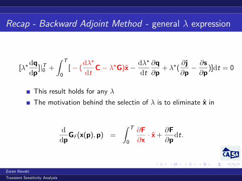
Recap - Backward Adjoint Method - general λ expression
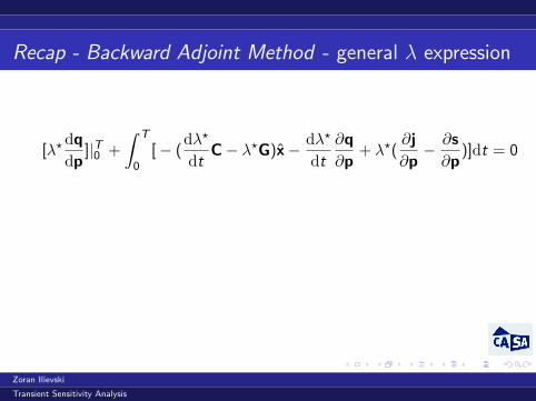
[λ?dq
dp]|T0 +
∫ T
0[− (
dλ?
dtC− λ?G)x− dλ?
dt
∂q
∂p+ λ?(
∂j
∂p− ∂s
∂p)]dt = 0
This result holds for any λ
The motivation behind the selectin of λ is to eliminate x in
ddp
Gf (x(p),p) =
∫ T
0
∂F
∂x· x +
∂F
∂pdt.
Zoran Ilievski
Transient Sensitivity Analysis

Recap - Backward Adjoint Method - general λ expression
[λ?dq
dp]|T0 +
∫ T
0[− (
dλ?
dtC− λ?G)x− dλ?
dt
∂q
∂p+ λ?(
∂j
∂p− ∂s
∂p)]dt = 0
This result holds for any λ
The motivation behind the selectin of λ is to eliminate x in
ddp
Gf (x(p),p) =
∫ T
0
∂F
∂x· x +
∂F
∂pdt.
Zoran Ilievski
Transient Sensitivity Analysis

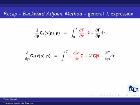
Recap - Backward Adjoint Method - general λ expression
ddp
Gf (x(p),p) =
∫ T
0
∂F
∂x· x +
∂F
∂pdt.
ddp
Gf (x(p),p) =
∫ T
0[−dλ?
dtC + λ?G]x +
∂F
∂pdt.
C?dλdt− G?λ = −(
∂F
∂x)?.
The natural conclusion is that this linear ’adjoint’ DAE is theconstraint on λ
Zoran Ilievski
Transient Sensitivity Analysis

Recap - Backward Adjoint Equation
This linear ’adjoint’ DAE is the constraint on λ
C?dλdt− G?λ = −(
∂F
∂x)?.
Zoran Ilievski
Transient Sensitivity Analysis

Recap - Backward Adjoint Equation
This linear ’adjoint’ DAE is the constraint on λ
The sensitivity can be rewritten in terms of λ if it satisfies theadjoint DAE
C?dλdt− G?λ = −(
∂F
∂x)?.
Zoran Ilievski
Transient Sensitivity Analysis
Recap - Backward Adjoint Equation
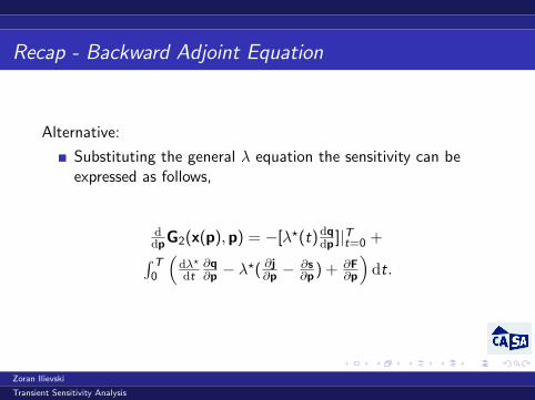
Alternative:
Substituting the general λ equation the sensitivity can beexpressed as follows,
ddpG2(x(p),p) = −[λ?(t)dq
dp ]|Tt=0 +∫ T0
(dλ?
dt∂q∂p − λ
?( ∂j∂p −∂s∂p) + ∂F
∂p
)dt.
Zoran Ilievski
Transient Sensitivity Analysis

Recap - Backward Adjoint Equation - initial conditions
−[λ?(t)(∂q∂x .x + ∂q∂p)]|Tt=0
x(t = T ) can be eliminated, if λ(T ) = 0
With this choice the sensitivity expression simplifies to,
ddp
G2(x(p),p) = λ?(0)[∂q
∂x(0).xDC +
∂q
∂p(0)] +∫ T
0
dλ?
dt
∂q
∂p− λ?(
∂j
∂p− ∂s
∂p) +
∂F
∂pdt. (5)
Zoran Ilievski
Transient Sensitivity Analysis

Recap - Backward Adjoint Equation - Summary
Standard transient analysis of forward system, initial conditionare set at t=0
d
dt[q(x(t,p),p)] + j(x(t,p),p) = s(t,p)
Solution of Backward Adjoint Equation
Each time integration step requires O(FN2) operations.
Initial condition are set at t=T, λ(T )=0
C?dλdt− G?λ = −(
∂F
∂x)?.
Zoran Ilievski
Transient Sensitivity Analysis
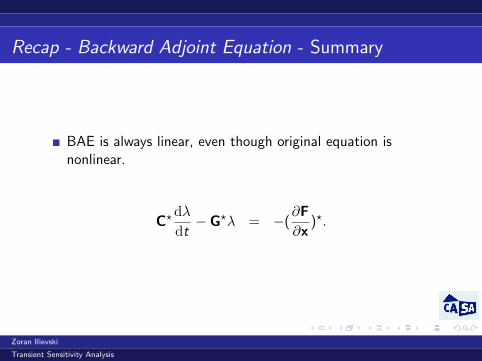
Recap - Backward Adjoint Equation - Summary
BAE is always linear, even though original equation isnonlinear.
C?dλdt− G?λ = −(
∂F
∂x)?.
Zoran Ilievski
Transient Sensitivity Analysis

Recap - Backward Adjoint Equation - Summary
substitution of λ values to obtain the observation sensitivity
The integrand at each time point requires O(PN + FP)operations and O(FPN) evaluations
ddp
G2(x(p),p) = λ?(0)[∂q
∂x(0).xDC +
∂q
∂p(0)] +∫ T
0
dλ?
dt
∂q
∂p− λ?(
∂j
∂p− ∂s
∂p) +
∂F
∂pdt.
Zoran Ilievski
Transient Sensitivity Analysis

Method Table
Direct Foward Backward AdjointCost O(min(F ,P),N2) + O(FPN) O(FN + FP) + O(FPN)
Usualy F << N
Zoran Ilievski
Transient Sensitivity Analysis

Talk Structure
Introduction
Recap Sensitivity
Examples and Results
Further Work
Zoran Ilievski
Transient Sensitivity Analysis

Backward Adjoint Equation - Reduction
C?dλdt− G?λ = −(
∂F
∂x)?.
Each time integration step requires an LU decomposition ofO(Nα)
α=2 for a sparce system and α=3 for a full system
This brings the total cost to O(Nα + FN2)
F << P, in practice
Quite a large cost for a large system, N.
What if we could project this system on to a n << Ndimensional subspace?
Zoran Ilievski
Transient Sensitivity Analysis
Proper Orthogonal Decomposition - Reduction
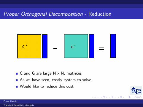
C and G are large N x N, matrices
As we have seen, costly system to solve
Would like to reduce this cost
Zoran Ilievski
Transient Sensitivity Analysis
Proper Orthogonal Decomposition - Reduction
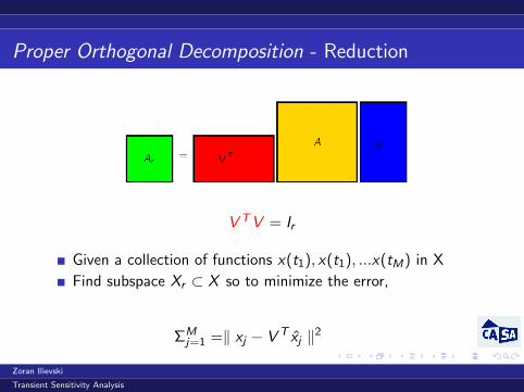
V TV = Ir
Given a collection of functions x(t1), x(t1), ...x(tM) in X
Find subspace Xr ⊂ X so to minimize the error,
ΣMj=1 =‖ xj − V T xj ‖2
Zoran Ilievski
Transient Sensitivity Analysis

Proper Orthogonal Decomposition - Reduction
Zoran Ilievski
Transient Sensitivity Analysis

Proper Orthogonal Decomposition - Reduction
For any system, in the state analysis we obtain,
X = [x(t1), x(t2)...x(tnsnapshots))] ∈ RnsnapshotsxN (6)
Next an SVD is computed giving,
X = V ΣU∗ ≈ VnΣnU?nn << N (7)
As long as the singular values decay rapidly the system can bereduced
xr = V ∗k x(t), xr ∈ Rn
Zoran Ilievski
Transient Sensitivity Analysis

Proper Orthogonal Decomposition - Reduction
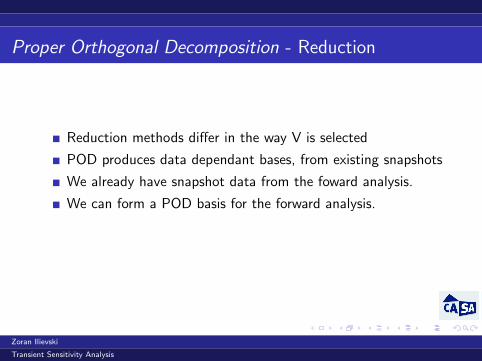
Reduction methods differ in the way V is selected
POD produces data dependant bases, from existing snapshots
We already have snapshot data from the foward analysis.
We can form a POD basis for the forward analysis.
Can we reduce the backward adjoint method with the samebasis?
Zoran Ilievski
Transient Sensitivity Analysis

Proper Orthogonal Decomposition - Reduction
Reduction methods differ in the way V is selected
POD produces data dependant bases, from existing snapshots
We already have snapshot data from the foward analysis.
We can form a POD basis for the forward analysis.
Can we reduce the backward adjoint method with the samebasis?
Zoran Ilievski
Transient Sensitivity Analysis

Backward Adjoint Equation - Reduction
Find a projection matrix, V to reduce the system to size n.
n << N
For highly non-linear circuits, POD is a good choice.
V is constructed from the left eigen vectors corresponding tothe most dominant singular values.
As long as the decay in singular values is rapid the system canbe reduced.
Zoran Ilievski
Transient Sensitivity Analysis
Backward Adjoint Equation - Reduction
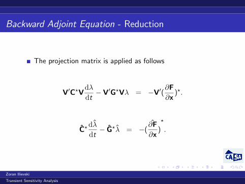
The projection matrix is applied as follows
V′C?Vdλdt− V′G?Vλ = −V′(
∂F
∂x)?.
C?dλdt− G?λ = −
ˆ(∂F
∂x)
?
.
Zoran Ilievski
Transient Sensitivity Analysis
Backward Adjoint Equation - Reduction
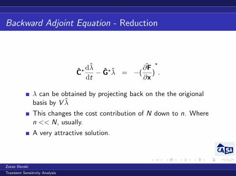
C?dλdt− G?λ = −
ˆ(∂F
∂x)
?
.
λ can be obtained by projecting back on the the origionalbasis by V λ
This changes the cost contribution of N down to n. Wheren << N, usually.
A very attractive solution.
Zoran Ilievski
Transient Sensitivity Analysis

Results(1) - Direct Forward
Sensitivity on Obf=Energy(I,R2) on R2, direct fowardmethod, is -3.068e-008
Zoran Ilievski
Transient Sensitivity Analysis

Results(1) - Direct Forward
Sensitivity Obf=Energy(I,R2) on R2, backward adjointmethod, is -3.068e-008
Previous result was -3.068e-008
Promising result
Zoran Ilievski
Transient Sensitivity Analysis

Results(2) - Reduction Example
length of R2 dG/dP dG/dP with POD
0.02 −0.235x10⁻¹⁰ −0.235x10⁻¹⁰
0.021 −0.247x10⁻¹⁰ −0.247x10⁻¹⁰
0.022 −0.256x10⁻¹⁰ −0.256x10⁻¹⁰
Zoran Ilievski
Transient Sensitivity Analysis
Results(3) - Industrial Singular Value Analysis
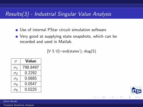
Use of internal PStar circuit simulation software
Very good at supplying state snapshots, which can berecorded and used in Matlab.
[V S U]=svd(states’); diag(S)
σ Value
σ1 798.8497
σ2 0.2292
σ3 0.0885
σ4 0.0547
σ5 0.0225
Zoran Ilievski
Transient Sensitivity Analysis

Results(3) - Industrial Example
The rapid decay is singular values is promising, it shows a nicePOD basis can be formed.
Zoran Ilievski
Transient Sensitivity Analysis

Talk Structure
Introduction
Recap Sensitivity
Examples and Results
Further Work
Zoran Ilievski
Transient Sensitivity Analysis

Conclusions and Further Work
We have written the BAE in forward form,
We use again the x(T-t) data in the state analysis, for theobservation function.
Form a POD bases for the state analysis.
Attempt to apply the same pod bases to the backward step.
Zoran Ilievski
Transient Sensitivity Analysis

Conclusions and Further Work
Further Work
For a simple circuit, we have had some success.
But were we just lucky.
Can we apply the POD basis on all circuits?
Collaborative work on the thory behind the application ofPOD is being carried out on this at Wuppertal.
We are aiming to submit an abstract for SCEE 2008 and apaper in the proceedings with the subject on POD for BAEmethods.
Zoran Ilievski
Transient Sensitivity Analysis

The End
THE END
Zoran Ilievski
Transient Sensitivity Analysis

Problem Description
The task is to reduce the Tline and then plug it back in tothe system.
The important requirement is to keep the nodes V1 and V2
safe.
Figure: Circuit with the Transmission Line
Zoran Ilievski
Transient Sensitivity Analysis
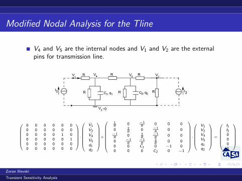
Modified Nodal Analysis for the Tline
V4 and V5 are the internal nodes and V1 and V2 are the externalpins for transmission line.
0BBBBB@0 0 0 0 0 00 0 0 0 0 00 0 0 0 1 00 0 0 0 0 10 0 0 0 0 00 0 0 0 0 0
1CCCCCA·
0BBBBBB@V1
V2
V4
V5q1q2
1CCCCCCA+
0BBBBBBB@
1R
0 −1R
0 0 0
0 2R
0 −1R
0 0−1R
0 3R
−1R
0 0
0 −1R
−1R
3R
0 00 0 C1 0 −1 00 0 0 C2 0 −1
1CCCCCCCA·
0BBBBB@V1V2V4V5q1q2
1CCCCCA =
0BBBBB@I1I20000
1CCCCCA
Zoran Ilievski
Transient Sensitivity Analysis

AMOR
The AMOR is an Arnoldi based algorithm which is usedPRIMA techniques inside to reduced the dynamical system.
The form which AMOR accepts is like this:{Bu = Ex + Kx ,y = Cx .
Zoran Ilievski
Transient Sensitivity Analysis

AMOR
bellow figure shows how we can define the AMOR input forthis TLINE.
In block form we have:
(0 00 E
)·(
ux
)+
(D C−B K
)·(
ux
)=
(y0
)Zoran Ilievski
Transient Sensitivity Analysis

AMOR
What if the T-Line is terminated with a capacitor?
Can this submodel be completely reduced?
Zoran Ilievski
Transient Sensitivity Analysis


![2016-10-12 Law v Ilievski [2016] ACTSC 291€¦ · Web viewTitle: 2016-10-12 Law v Ilievski [2016] ACTSC 291 Created Date: 10/12/2016 5:45:00 AM Other titles: 2016-10-12 Law v Ilievski](https://static.fdocuments.in/doc/165x107/6075790bb662e06fc0077747/2016-10-12-law-v-ilievski-2016-actsc-291-web-view-title-2016-10-12-law-v-ilievski.jpg)