Train Detection by Magnetic Field Sensing

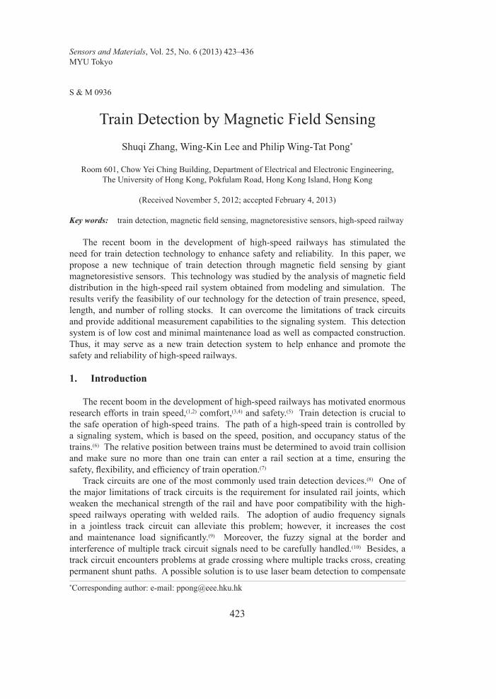
Sensors and Materials, Vol. 25, No. 6 (2013) 423–436MYU Tokyo

S & M 0936

*Corresponding author: e-mail: [email protected]

423

Train Detection by Magnetic Field SensingShuqi Zhang, Wing-Kin Lee and Philip Wing-Tat Pong*

Room 601, Chow Yei Ching Building, Department of Electrical and Electronic Engineering,The University of Hong Kong, Pokfulam Road, Hong Kong Island, Hong Kong

(Received November 5, 2012; accepted February 4, 2013)

Key words: traindetection,magneticfieldsensing,magnetoresistivesensors,high-speedrailway

The recent boom in the development of high-speed railways has stimulated the need for train detection technology to enhance safety and reliability. In this paper, we propose a new technique of train detection through magnetic field sensing by giantmagnetoresistivesensors.Thistechnologywasstudiedbytheanalysisofmagneticfielddistribution in the high-speed rail system obtained from modeling and simulation. The results verify the feasibility of our technology for the detection of train presence, speed, length, and number of rolling stocks. It can overcome the limitations of track circuits and provide additional measurement capabilities to the signaling system. This detection system is of low cost and minimal maintenance load as well as compacted construction. Thus, it may serve as a new train detection system to help enhance and promote the safety and reliability of high-speed railways.

1. Introduction

The recent boom in the development of high-speed railways has motivated enormous research efforts in train speed,(1,2) comfort,(3,4) and safety.(5) Train detection is crucial to the safe operation of high-speed trains. The path of a high-speed train is controlled by a signaling system, which is based on the speed, position, and occupancy status of the trains.(6) The relative position between trains must be determined to avoid train collision and make sure no more than one train can enter a rail section at a time, ensuring the safety,flexibility,andefficiencyoftrainoperation.(7)

Track circuits are one of the most commonly used train detection devices.(8) One of the major limitations of track circuits is the requirement for insulated rail joints, which weaken the mechanical strength of the rail and have poor compatibility with the high-speed railways operating with welded rails. The adoption of audio frequency signals in a jointless track circuit can alleviate this problem; however, it increases the cost and maintenance load significantly.(9) Moreover, the fuzzy signal at the border and interference of multiple track circuit signals need to be carefully handled.(10) Besides, a track circuit encounters problems at grade crossing where multiple tracks cross, creating permanent shunt paths. A possible solution is to use laser beam detection to compensate

424 Sensors and Materials, Vol. 25, No. 6 (2013)

for the shortage; however, it would greatly increase the cost of construction.(11) Several factors such as rust, compacted leaf residue, and wet tunnels may cause abnormal operationofthetrackcircuit.Theaxlecounterisalsoawidelydeployedtraindetectiondevice, which counts the number of wheel pairs passing the detection point at the start of a section.(12)Thereareseveraldisadvantagesofaxlecounters.Inthecasewhentheaxlecounterlosesitsmemoryoftheaxlenumber,amanualresetisnecessarytorestartthe system. This introduces human factors as a source of unreliability. Second, axlecounterscannotworkwithafail-safeprinciple.Moreover,axlecountershaveaproblemwhen the wheels stop right at the counters. It may also regard the electromagnetic brakingdevicesonhigh-speedtrainsasaxlesbymistake.(13) Some researchers suggest acombineduseoftrackcircuitandaxlecounter;however,itdoesnothelpaddressthedisadvantages mentioned above.(14) There are other types of detection methods. Sense coils, inductive loops, and trip switches can only detect trains in motion, and they cannot detect stationary objects.(15) The EVA system(15) applies infrared beam sensors for stationarytraindetection,whichresultsinsignificantexpenses.Otherdetectionsystemsinclude vibration detection,(16–18) passive infrared and ultrasonic detection, video imaging, sound detection of locomotive horn, communication-based train detection with onboard Global Positioning System (GPS) and wayside radio links.(15) However, these methods eitherrequireexpensiveequipmentandlargemaintenanceloadortheyaresusceptibletointerference from various factors such as light condition and environmental temperature. Thus, a new detection technique is needed for high-speed railways, which require a higher safety standard and a more stringent signaling. In this paper, a new train detection technique for high-speed railways by magnetic field sensingwith giantmagnetoresistive (GMR) sensors is proposed. Magnetic fieldsensing has been applied in vehicle detection and car speed measurement.(19) Since railway trains contain ferromagnetic materials, it is possible to develop a similar method for train detection. The new technique eliminates the need for insulated rail joints. It makesuseof themagneticfieldgenerated fromtheoverheadcontact systemsofhigh-speed rails and thus it is compatible with all high-speed railway systems. Moreover, this technique enables continuous detection at grade crossing, and it is applicable to both moving and stationary trains. It offers additional features: it can measure the number of rolling stocks, train speed, and length, which may enable us to obtain the train identity and statistics. GMR sensors offer the best performance in terms of cost, size, and energy consumption among various magnetometers such as anisotropic magnetoresistance (AMR)sensors,fluxgate,superconductingquantuminterferencedevices(SQUIDs),andelectron-spin-resonance magnetometers.(20) These advantages are beneficial for large-scale application and long-term usage as required for train detection in railways.

2. ModelingandSimulation

The modeling and simulation were carried out by the finite element method inANSYS Maxwell. The entire model is divided into two parts: the electrical circuitfor power supply and the train. The circuit consists of overhead contact lines for power supply, which include a catenary wire and a contact wire, and the return circuit for returning current including one negative feeder, one return conductor, two rails,

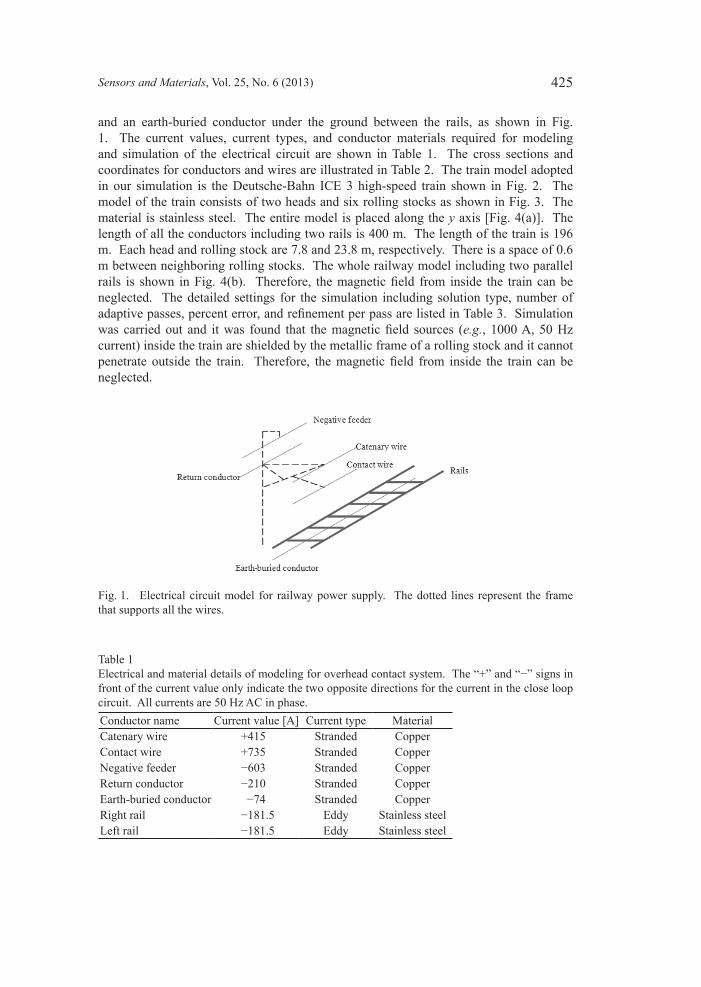
Sensors and Materials, Vol. 25, No. 6 (2013) 425

and an earth-buried conductor under the ground between the rails, as shown in Fig. 1. The current values, current types, and conductor materials required for modeling and simulation of the electrical circuit are shown in Table 1. The cross sections and coordinates for conductors and wires are illustrated in Table 2. The train model adopted in our simulation is the Deutsche-Bahn ICE 3 high-speed train shown in Fig. 2. The modelofthetrainconsistsoftwoheadsandsixrollingstocksasshowninFig.3.Thematerial is stainless steel. The entire model is placed along the yaxis[Fig.4(a)].Thelength of all the conductors including two rails is 400 m. The length of the train is 196 m. Each head and rolling stock are 7.8 and 23.8 m, respectively. There is a space of 0.6 m between neighboring rolling stocks. The whole railway model including two parallel rails is shown inFig.4(b). Therefore, themagneticfield from inside the train canbeneglected. The detailed settings for the simulation including solution type, number of adaptivepasses,percenterror,andrefinementperpassarelistedinTable3.Simulationwas carriedout and itwas found that themagneticfield sources (e.g., 1000 A, 50 Hz current) inside the train are shielded by the metallic frame of a rolling stock and it cannot penetrate outside the train. Therefore, themagneticfield from inside the train canbeneglected.

Fig. 1. Electrical circuit model for railway power supply. The dotted lines represent the frame that supports all the wires.

Table 1Electricalandmaterialdetailsofmodelingforoverheadcontactsystem.The“+”and“−”signsinfront of the current value only indicate the two opposite directions for the current in the close loop circuit. All currents are 50 Hz AC in phase.Conductor name Currentvalue[A] Current type MaterialCatenary wire +415 Stranded CopperContact wire +735 Stranded CopperNegative feeder −603 Stranded CopperReturn conductor −210 Stranded CopperEarth-buried conductor −74 Stranded CopperRight rail −181.5 Eddy Stainless steelLeft rail −181.5 Eddy Stainless steel

-


Table 2Cross sections and coordinates for modeling of overhead contact system.Conductor name Cross section Radius[m] Coordinates (x, z)[m]Catenary wire 0.00707 (2, 9.5)

Contact wire 0.006 (0, 5.4)

Negative feeder 0.006 (0, 7.2)

Return conductor 0.006 (3, 5.4)

Earth-buried conductor 0.006 (0, −0.2)

Left rail (0.7875, 0)

Right rail (−0.7875, 0)

Fig. 2. (a) Deutsche-Bahn ICE 3 high-speed train and (b) structural model of Deutsche-Bahn ICE 3 from Google sketchup.

Fig. 3. Train model in different views.

(a) (b)


Fig.4. Overall3Dviewofcompletemodel:(a)establishedmodelinMaxwelland(b)illustrationof railway structure including two parallel rails.

3. SimulationResultsandDiscussion

3.1 Effectoftrainpresenceonmagneticfielddistribution ThesimulationresultinFig.5showsthemagneticfielddistributiononthexz plane. Themagneticfield is strongestaround thewiresandconductors, and itdecaysas it isfarther away from these sources. By comparing with the situation without a train (the right half of the simulation), it can be observed that the magnetic field distributionbecomes dense and strong above the train, while sparse and weak at the sides of the train. This leads to the phenomenon that the presence of the trainwarps themagnetic fieldgeneratedfromthewiresandconductors—thetrainpresencestrengthensthefieldabovethetrainandweakensthefieldatthesidesofthetrain.Figure6showstheeffectoftrainpresenceonthemagneticfielddistributioninthetopview. Theplaneselectedisrightabove the train in the xy plane. The outline of the train is overlapped onto the simulation result for better observation. It can be seen that in the area above the train, the magnetic fieldbecomesstrongerthanintheregionsnearby.Atthesideofthetrain,themagneticfieldisweakened.FromthesimulationresultsinbothFigs.5and6,thepresenceofatrainwarpsthemagneticfieldgeneratedfromthewiresandconductors.Theeffectofthewarpingabovethetrainisoppositetothatatthesidesofthetrain.Themagneticfieldbecomesstrongerabovethetrainwhereasthemagneticfieldisweakenedatthesides.

(a) (b)

Table 3Settings and parameters for simulation.Solution type Eddy currentModel 3DAnalysis setup Passes 8

Percent error 1Refinementperpass 30Minimum number of passes 2Minimum converged passes 1Adaptive frequency 50 Hz


Fig.5. Magneticfielddistributiononxz plane (y = 0). The right half shows the distribution of magnetic fieldwithout a train. The comparison between the left and right half shows that themagnetic field above the train is strengthened,while the fields at the two sides of the train areweakened.

Fig.6. Magneticfielddistributionfromtopviewofthemodel.Thechosenplaneisinthexy plane (z = 4), i.e., the plane right above the train. The outline of the train is denoted and the lines across the plot are the conductors including catenary wires, return conductors, and negative feeders.

Figures 7 and 8 are plots of the magnetic field variation along the rail in the y direction. Theplotstartsfromoneendof the trainandextends to400mtocover theentire model of the train and the railway system. From the magnetic field variationabovethetrainshowninFig.7,themagneticfieldintheregionofthetrain(0–196m)is approximately 80 µT higher than that in the regionwithout the train (196–400m).FromthemagneticfieldvariationatthesideofthetrainshowninFig.8,itcanbeseenthatthemagneticfieldintheregionofthetrain(0–196m)isapproximately40µTlowerthan that in the region without the train (196–400 m). An interesting feature is that there aresomepulsesinthemagneticfieldvariation.Thesepulsesoccuratthegapsbetweenrolling stocks. At these gaps, there are no ferromagnetic materials, and thus, there are


suddenchangesinthemagneticfield.Thissignaturepatterncanbeusedforcountingthenumberofrollingstocksasexplainedin§3.3.2. Fromtheaboveresults,asatrainpasses,themagneticfieldexhibitssuchpatternsofvariation and these can provide effective evidence for train presence detection. Since GMRsensorscansenseamagneticfieldfromDCtoover1MHz,stationarytrainscanalso be detected.

3.2 Best positions for sensors Todeterminewheretoplacethemagneticfieldsensors,afewpositionswereanalyzedfor their suitability for placing sensors for train detection. The positions were chosen from above the train (A–C) and at the sides of the train (D–I) as shown in Fig. 9. Figures 10–12illustratethewarpingofthemagneticfieldduetothetrainalongthey direction from0to400matthesepositions.FromFig.10,itcanbeseenthatthemagneticfieldvariation differs at different heights above the train and it is larger for positions closer to the train. As it goes farther from the train in the z direction, the variation becomes insignificant.FromFig.11,itcanbeseenthatatthesideofthetrain,themagneticfieldvariation is larger for positions E and F. From Fig. 12, it can be seen that at the side of thetrain,themagneticfieldvariationislargerforpositionsclosertothetrain.Whenitisfarther away from the train in the x direction, the variation becomes smaller.

Fig.7. Magneticfieldvariation along they direction (x = 0, z = 4) above the train. The train rangesfrom0to196mintheplot.Thesignaturechangeinmagneticfieldcanbeobservedatthegaps between rolling stocks.

Fig.8. Magneticfieldintensityvariationalongthey direction (x = 2, z = 4) at the side of the train. The line lies in the y direction and passes (2, 0, 4). The train ranges from 0 to 196 m in the plot.


Fig.10(left).MagneticfieldvariationabovethetrainatpositionsA–C:A,alongthelinepassing(0,0, 4); B, along the line passing (0, 0, 4.5); and C, along the line passing (0, 0, 5).Fig.11(right).MagneticfieldvariationatthesideofthetrainatpositionsD–F:D,alongthelinepassing (2, 0, 2); E, along the line passing (2, 0, 3); and F, along the line passing (2, 0, 4).

Fig.9. Illustrationof thepositionsselected for investigating themagneticfieldvariation. Dotsare positions above the train and circles are positions at the side of the train. A–I correspond to the plots marked by A–I in Figs. 11–13. The positions A–C were chosen to illustrate the difference in themagneticfieldvariationatdifferentverticalheightsabovethetrain.ThepositionsD–Fwerechosentoillustratethedifferenceinthemagneticfieldvariationatdifferentverticalheightsattheside of the train. The positions E and G–I were chosen to illustrate the difference in the magnetic fieldvariationatdifferenthorizontaldistancesfromthesideofthetrain.


Fig.12.MagneticfieldvariationatthesideofthetrainatpositionsEandG–I:E,alongthelinepassing (2, 0, 3); G, along the line passing (2.5, 0, 3); H, along the line passing (3, 0, 3); and I, along the line passing (3.5, 0, 3).

From the above observation anddiscussion, thewarping of themagneticfield dueto the train presence can be summarized as follows: above the train, the warping is stronger at positions closer to the train in the z direction; at the side of the train, the warping is stronger at the vertical levels of z = 3 and z = 4 than at z = 2, and it is stronger at positions with a shorter horizontal distance from the train. Therefore, the highlighted regions including positions C, E, and F in Fig. 13 are better for placing sensors because thewarpingofthemagneticfieldintheseregionsisstrongerthanintheotherregions,and thus, a better signal-to-noise ratio is obtained. These regions can be accessed for placingsensorswithasimplestructureasshowninFig.14.Onthebasisofthefindingsdescribed in §§ 3.1 and 3.2, the magnetic field measurement can be applied to thedetection of a set of parameters concerning the train: presence, number of rolling stocks, speed, and length.


3.3 Detection of trains3.3.1 Detection of train presence Asdiscussed in§3.1, themagneticfieldabove the train ishigher than in thecasewithoutthetrain(Fig.7),whereasthemagneticfieldisloweratthesideofthetrainthanin the case without the train (Fig. 8). Therefore, when a train passes by the sensor or stopsnext to the sensor, themagneticfieldmeasuredbecomeshigher (if the sensor isabove the train) or lower (if the sensor is by the side of the train) than the normal level. Therefore, the presence of a train can be detected. When the train departs from the sensor,themagneticfieldreturnstothenormallevelagain.

3.3.2Detectionofnumberofrollingstocks In addition to the presence of a train, themagnetic field signatures indicating thegaps between rolling stocks (discussed in § 3.1) canprovide information for countingthe number of rolling stocks. The number of rolling stocks is one plus the number of signatures detected by the sensor during the passing of the train. If two sensors are placed at the two ends of a track section, the number of rolling stocks that enter and

Fig. 14. Sensors placed (a) above the train and (b) at side of the train. The highlighted component enclosed by a dotted line at the end of the bar is the GMR sensor.

(a) (b)

Fig. 13. Regions for placing magnetic sensors. The light-grey rectangular regions are better places forsensorswithstrongerwarpingeffectofmagneticfieldfromthetrain.


Fig. 15. Illustration for speed measurement with one sensor. A train is passing by sensor A from time t1 to t2. The situations at (a) t1 and (b) t2areshown.Thecomponentsmarkedby●aretheGMR sensors. The arrow indicates the traveling direction of the train. The waveforms below are thecorrespondingmagneticfieldvariation.Itcanbeseenthatthefirstsignaturehappensatt1 and the second one occurs at t2.

(b)(a)

leave this section can be recorded and compared to see if the whole train has left the track section.

3.3.3 Detection of Speed There are two methods of speed detection. With one sensor and the known length of each rolling stock, the speed of the train can be deduced. As shown in Fig. 15, a train passesbysensorA,whichisplacedatpositionEdenotedinFig.9.Afterthefirstrollingstock travels past sensor A, the gap between the rolling stocks and, thus, its signature is detected by sensor A at time t1. After the second rolling stocks travel past sensor A, the second gap and, thus, its signature occur at time t2. If the length of each rolling stocks is given as L and the spacing between two rolling stocks is d, then the average speed v of the train in this duration is

v =L + 2 d

2

t2 − t1. (1)

The train speed can also be detected with two sensors placed along the rail. In this case, the length of the rolling stock does not need to be predetermined. As shown in Fig. 16, a train passes by sensors B and C, which are both placed at position E denoted in Fig. 9. Supposetheoccurrenceofthefirstsignatureistakenasthesignformeasuringthespeed,sensorBdetects itsfirst signature at time t3, and sensorCdetects itsfirst signature attime t4. The distance LBCbetweensensorsBandCisknown,andtheapproximatespeedof the train can be obtained as

v =LBC

t4 − t3. (2)


3.3.4 Detection of length If the train speed is known, the train length can be derived by measuring the duration for the entire train to travel past the sensor. As shown in Fig. 17, a train passes by sensor D, which is placed at position E. The head of the train passes the sensor at time t5, whereas the tail passes the sensor at time t6. SensorDwill detect themagneticfieldvariationowing to the train presence starting from time t5 until t6 when the train has left. If the speed of the train is v, the length of the train l will be

l = v(t6−t5). (3)

3.4 Fail-safe mechanism Fail-safeisanecessarypartofacompletetraindetectionsystem.Bydefiningproperlogiclevelsforthemagneticfield,ourtechniquecanbefail-safe. Thiscanberealizedwhen the sensor is placed at the side of the train, rather than above the train. Taking the magneticfieldvariationatpositionEasanillustration,theredlineatlevel40µTistakenas the reference line (Fig. 18). The comparator defines themagnetic field above thisreference line as logic “1”, and that below as logic “0”. When there is no train and the sensorworkswell,themagneticfieldmeasuredisabovethereferencelineandthusthecomparator outputs “1”, which indicates a proceed signal. In the presence of a train, the magneticfielddropstothelowerlevelandthecomparatoroutputs“0”,whichindicatesastopsignal.Ifthesensorfails,thereisnomagneticfielddetectedandthecomparatorwillkeepprovidingalogicaloutputof0indicatingastopsignal.Wedefinevariablea as the presence status of a train (“0” = no train, “1” = train presence), variable b as the working status of the sensor (“0” = fail, “1” = working), and s as the logical output of the comparator (“0” = occupied, “1” = unoccupied). The relation of a, b, and s is described using eq. (4) and the logic table is shown in Table 4.

s = a * b (4)

Fig.16. Illustration for speed measurement with two sensors. A train is passing sensor B and sensor C from time t3 to t4. The situations at (a) t3 and (b) t4 are shown. The components markedby●aretheGMRsensors.Thearrowindicatesthetravelingdirectionofthetrain.Thewaveformsbelowarethecorrespondingmagneticfieldvariation.Itcanbeseenthatatt3, sensor B hasitsfirstsignature,whileatt4,sensorChasitsfirstsignature.

(a) (b)


Fig. 17. Illustration of train length measurement with one sensor. A train is passing sensor D from time t5 to t6. The situations at (a) t5 and (b) t6 are shown. The arrow indicates the traveling directionofthetrain.Thewaveformsbelowarethecorrespondingmagneticfieldvariation.Itcanbe seen that the variation starts at t5 and ends at t6. This means that the entire train passes from t5 to t6.

(a) (b)

Fig.18.Mappingofanalogvalueofmagneticfieldintensitytologics“1”and“0”.Theredlineat40µTischosentobethereferenceline.Thevalueabovethereferencelineislogic“1”,belowis

It can be seen that the detection system produces a logic “1”, i.e., a “proceed” aspect signal, only in the case when there is no train and the device works normally. The signal is “stop” for all other cases including the cases when the sensor fails. This meets the fail-safe principle.

Table 4Logic table for different cases of train presence and sensor working status. “a”, “b”, and “s” are the presence status of a train, the working status of the sensor, and the logic output of the comparator, respectively.Cases a b s SignalNo train & device works 0 1 1 ProceedWith train & device works 1 1 0 StopNo train & device fails 0 0 0 StopWith train & device fails 1 0 0 Stop


4. Conclusions

The new technique for train detection overcomes some of the shortcomings of track circuits. Firstly, it does not require special features of tracks, such as insulated rail joints; secondly, it does not lose effectiveness at grade crossing. Moreover, the detection is immune to factors such as rust and wet environment. The new technique also has advantages in terms of cost, size, and energy consumption. GMR sensors cost just a few US dollars each. A GMR sensor is only a few mm in size, which leaves plenty of margin for construction space. Its power consumption is only around 10 mW(21) and, thus, a battery can last for a long time without maintenance. The new train detection systemhasarelativelylowcomplexitybecauseitdoesnotrequiretransmitterdevicesorwayside controllers. Unlike some of the train detection methods that require additional processingoftherawdetectiondata,forexample,theimagevideodetectiontechnique,theGMRsensorconvertsthemagneticfieldmeasurementintoelectricalsignaldirectly.This technique is proposed and described in detail, and its principle and feasibility are verified by modeling and simulation in this study. Its advantages over the existingmethods make it promising for train detection in modern high-speed railway systems.

References

1 W. M. Hwang and Y. L. Huang: Trans. Can. Soc. Mech. Eng. 29 (2005) 41. 2 A. K. W. Ahmed, C. Liu and I. Haque: Trans. Can. Soc. Mech. Eng. 20 (1996) 365. 3 Y. Ravalard, D. Coutellier and S. Masfrand: Trans. Can. Soc. Mech. Eng. 18 (1994) 269. 4 M. A. Soliman, M. S. Kaldas, D. C. Barton and P. C. Brooks: IJETI 2 (2012) 85. 5 J. I. Real, L. Montalban, T. Real and V. Puig: J. Vibroeng. 14 (2012) 813. 6 D.Chen,W.XieandC.Qian:ForeignElectron.Meas.Technol.24 (2005) 9. 7 J. Gonzalez, C. Rodriguez, J. Blanquer, J. M. Mera, E. Castellote and R. Santos: J. Adv.

Transp. 44 (2010) 53. 8 J. W. Palmer: RSCS 2012 (2012) 60. 9 N. Nikolov and N. Nedelchev: IEEE Proc. Electr. Power Appl. 152 (2005) 1049. 10 A. Taguti: Electr. Eng. Jpn. 127 (1999) 64. 11 F. T. Pascoe: United States Patent No. 3725699 (1973). 12 X. Wu: RSCE 3 (2006) 43. 13 H. Uebel: United States Patent No. 6565046 (2003).14 L.L.McAllister:EuropeanPatentSpecificationNo.1295775(2011). 15 A. A. Carroll, J. E. Gordon, R. P. Reiff and S. E. Gage: Proc. Seventh International

Symposium on Railroad-Highway Grade Crossing Research and Safety: Getting Active at Passive Crossings (ARRB Group Limited, Melbourne, 2002) pp. 36–49.

16 D. Guzas: J. Vibroeng. 12 (2010) 642. 17 J. I. Real, T. Asensio, L. Montalban and C. Zamorano: J. Vibroeng. 14 (2012) 880. 18 J. I. Real, T. Asensio, L. Montalban and C. Zamorano: J. Vibroeng. 14 (2012) 408. 19 J. Pelegri, J. Alberola and V. Llario: Proc. 28th IECON (IEEE, Sevilla, 2002) pp. 1693–1695. 20 NVE Corp: Low-Field Magnetic Sensing with GMR Sensors, http://www.nve.com/

Downloads/lowfield.pdf(accessedonJanuary2013). 21 NVE Corp: AA and AB-Series Analog Sensors, http://www.nve.com/Downloads/

analog_catalog.pdf (accessed on May 2012).

Train Detection by Magnetic Field Sensing

Documents

Transcript of Train Detection by Magnetic Field Sensing