Detection of Magnetic Nanoparticles for Bio-sensing ...
163
Detection of Magnetic Nanoparticles for Bio-sensing Applications A DISSERTATION SUBMITTED TO THE FACULTY OF THE GRADUATE SCHOOL OF THE UNIVERSITY OF MINNESOTA BY LIANG TU IN PARTIAL FULFILLMENT OF THE REQUIREMENTS FOR THE DEGREE OF DOCTOR OF PHILOSOPHY JIAN-PING WANG, ADVISOR JUNE, 2013
Transcript of Detection of Magnetic Nanoparticles for Bio-sensing ...

Detection of Magnetic Nanoparticles for Bio-sensing Applications
A DISSERTATION
SUBMITTED TO THE FACULTY OF THE GRADUATE
SCHOOL
OF THE UNIVERSITY OF MINNESOTA
BY
LIANG TU
IN PARTIAL FULFILLMENT OF THE REQUIREMENTS
FOR THE DEGREE OF
DOCTOR OF PHILOSOPHY
JIAN-PING WANG, ADVISOR
JUNE, 2013

© Liang Tu 2013

i
Acknowledgements
I am very much delighted to have this chance to thank those people who
supported and helped me. First of all, I would like to thank my advisor, Professor
Jian-Ping Wang, for his sharing of scientific mind, introducing me to the research
field of magnetic materials and supervising me to do this exciting project. The
discussion with him was invaluable and guided me to passionately explore amazing
science in this topic.
I would also like to acknowledge the input and advice from Professor Randall
Victora, Beth Stadler and Jack Judy during my work and stay in the center for
Micromagnetic and Information Technollogies (MINT), which builds a solid
foundation for me in the field of magnetism and magnetic materials.
I am thankful to my dissertation committee members Professor Sang-Hyun Oh,
Jizhen Lin, Anand Gobinath, Beth Stadler, Rhonda Franklin, and Walter Low for
their time, help and effort of serving in my committee.
This work was also supported by an OTC Innovation grant from the
University of Minnesota and National Science Foundation BME 0730825 and
Institute of Engineering in Medicine at University of Minnesota. Parts of this work
were carried out using the Characterization Facility which receives partial support
from NSF through the NSF Minnesota MRSEC Program under Award Number
DMR-0819885 and NNIN program.
It has been an enjoyable experience with the past and current members of
Professor Wang’s group. I would like to thank all the group members for their
valuable discussion and friendly feedback.
Finally, I would like to express my love and thanks to my parents and my
friends. Without their love, support and advice, I would have never gone so far.

ii
Dedication
With gratitude to my parents.

iii
Abstract
Superparamagnetic Nanoparticles (MNPs) are used as probes to detect biomarkers
(protein, DNA, etc.) by using a search coil based scheme for volume detection and by using
a Giant Magneto-Resistance (GMR) sensor for surface detection.
In search coil detection scheme, a low frequency field is applied to saturate the
MNPs and a high frequency field is applied to modulate the nonlinearity of the
magnetization into the high frequency region where the noise floor is lower. Under an ac
magnetic field, MNPs above certain hydrodynamic size (for Iron Oxide is around 20nm)
will experience physical rotation called Brownian relaxation. 1By studying the phase
information of the mixing frequencies, the Brownian relaxation time can be monitored in
real time thus dynamic bio-molecular interaction can be recovered. The Néel and Brownian
relaxation of MNPs with different magnetic and hydrodynamic properties has been
investigated by using a different DC bias field and AC field frequency. The specific
response from each MNP can be used as magnetic identification in nano-scale application.
A Giant Magneto-Resistance (GMR) sensor array is also used for MNPs detection.
Compared with the search coil, GMR sensor is more sensitive but requires surface
modification for bio- molecular detection. A low-noise Printed Circuit Board is designed
and assembled to implement Wheatstone bridge, multiplexing function, and signal
amplification. An AC field is applied to the entire sensor array while an AC current is
flowing through a specific sensor. The sensor response will generate mixing frequency
terms as the multiplication of field frequency and current frequency. All the active sensors
printed with specific capture antibodies are scanned sequentially, recorded in real time, and
compared with the reference sensor which is covered by a thick protection layer. Signal to
noise ratio for the integrated system is studied by considering the noise contribution from all
components.

iv
Table of Contents
Acknowledgements ........................................................................................................... i
Dedication ......................................................................................................................... ii
Abstract ............................................................................................................................ iii
List of Figures ................................................................................................................ viii
List of Tables ................................................................................................................ xvii
Chapter 1 Introduction .................................................................................................. 1
1.1 Ferromagnetism in a material .............................................................................................. 1
1.2 Superparamagnetism ........................................................................................................... 2
1.3 Magnetic Spin Relaxation ..................................................................................................... 6
1.3.1 Electron spin dynamics......................................................................................... 6
1.3.2 Static magnetization............................................................................................. 6
1.3.3 Dynamic magnetization........................................................................................ 6
1.3.4 Brown’s equation ................................................................................................. 7
1.3.5 Solution to Brown’s equation............................................................................... 8
1.3.6 Néel relaxation time ............................................................................................. 9
1.4 AC susceptibility of MNPs ................................................................................................... 10
1.4.1 Brownian relaxation ........................................................................................... 10
1.4.2 Total relaxation .................................................................................................. 11
1.4.3 Debye model ...................................................................................................... 12
1.5 MNPs characterization ....................................................................................................... 14
1.5.1 VSM .................................................................................................................... 14
1.5.2 SEM and TEM ..................................................................................................... 15
1.5.3 DLS ...................................................................................................................... 17
Chapter 2 Mixing Frequency Method ......................................................................... 19

v
2.1 Search-coil Detection ......................................................................................................... 19
2.2 MNPs magnetic flux in coil (equation and simulation) ........................................................ 21
2.3 Mixing Frequency Method ................................................................................................. 25
2.3.1 Introduction to the Mixing Frequency Method ................................................. 25
2.3.2 Theory of the Mixing Frequency Method .......................................................... 27
2.3.3 Experimental setup ............................................................................................ 29
2.3.4 MNPs detection .................................................................................................. 30
2.3.5 Theoretical Limit of Detection (LOD) by Mixing Frequency Method ................. 33
2.4 Multi-tone Mixing-frequency method ................................................................................ 34
2.5 Relaxation modulation by field amplitude ......................................................................... 38
2.5.1 Brownian relaxation modulation ....................................................................... 38
2.5.2 Néel relaxation modulation ............................................................................... 43
2.5.3 Simulation of relaxation modulation ................................................................. 47
Chapter 3 Application of Mixing Frequency Method ................................................. 51
1. 1 Brownian Relaxation Measurement ................................................................................... 51
3.1.1 Brownian Relaxation Measurement by Mixing Frequency Method .................. 51
3.1.2 Real-time Brownian Relaxation Measurement .................................................. 52
3.2 MNP coloring...................................................................................................................... 56
3.2.1 MNP responses along frequency ....................................................................... 56
3.2.2 MNP coloring simulation .................................................................................... 60
3.2.3 MNP coloring using amplitude of magnetization ............................................... 64
3.2.4 MNP coloring using amplitude and phase of magnetization ............................. 68
3.2.5 MNP coloring by adding a static field ................................................................. 72
3.3 Bulk material measurement ............................................................................................... 75

vi
3.4 Thin film measurement ...................................................................................................... 76
3.5 Magnetosome measurement ............................................................................................. 79
3.6 Viscosity measurement ...................................................................................................... 82
Chapter 4 Measurement of GMR ................................................................................ 85
1. 1 GMR Sensor ........................................................................................................................ 85
1. 2 Measurement Scheme........................................................................................................ 86
4.1.1 Anderson Loop ................................................................................................... 87
4.1.2 Wheatstone Bridge ............................................................................................ 88
4.2 Mixing frequency measurement ......................................................................................... 88
4.3 Measurement Results ........................................................................................................ 92
4.4 GMR Model ........................................................................................................................ 95
4.5 GMR Sensitivity .................................................................................................................. 99
4.6 GMR Noise ....................................................................................................................... 100
4.7 GMR Drift ......................................................................................................................... 103
4.8 Optical Effects .................................................................................................................. 104
4.9 Detection Circuit .............................................................................................................. 110
4.9.1 DAQ: NI USB-6289 ........................................................................................ 112
4.9.2 Low Pass Filter .................................................................................................. 112
4.9.3 Input Voltage Follower ..................................................................................... 113
4.9.4 Multiplexer ....................................................................................................... 115
4.9.5 Output Voltage Amplifier ................................................................................. 118
4.10 System Noise Analyze ....................................................................................................... 120
4.11 Other development .......................................................................................................... 124
4.11.1 Microcontroller Developments ........................................................................ 124
4.11.2 Demodulation circuits ...................................................................................... 126
4.11.3 Function Generating Circuit ............................................................................. 127

vii
Chapter 5 Conclusion and Outlook ........................................................................... 129
5.1 Conclusion ........................................................................................................................ 129
5.2 Outlook ............................................................................................................................ 129
Bibliography ................................................................................................................. 131
Appendix ...................................................................................................................... 134
1. 1 FMR .................................................................................................................................. 134
viii
List of Figures
Figure 1-1 Comparison of magnetization curves of Ferro, Para and
Superpara-magnetism .................................................................................................. 4
Figure 1-2 Single domain size, Dcrit and magnetic stability size or the
superparamagnetic limit at room temperature, Dsp for some common ferromagnetic
materials. ..................................................................................................................... 5
Figure 1-3 schematic of the magnetic moment of a MNP in relative to the
applied field. .............................................................................................................. 11
Figure 1-4 An example of measurement of real and imaginary part of ac
susceptibility along frequency. .................................................................................. 14
Figure 1-5 schematic of a VSM and an example of measured hysteresis curve.
................................................................................................................................... 15
Figure 1-6 schematic of a TEM. ...................................................................... 16
Figure 2-1 detection ranges of various magnetic field sensors ........................ 19
Figure 2-2 sensitivity of various magnetic field sensors along frequency. ...... 20
Figure 2-3 Schematic of traditional susceptometer setup. ............................... 21
Figure 2-4 Magnetic dipole model ................................................................... 22
Figure 2-5 Magnetic moment of a single MNP ............................................... 24
Figure 2-6 Schematic of magnetization of MNPs under an ac field, in time and
frequency domain. ..................................................................................................... 26
Figure 2-7 Schematic of experimental setup. .................................................. 29
Figure 2-8 M-H loop of Fe40Co60 MNPs sample at room temperature
measured by SQUID. ................................................................................................. 30
Figure 2-9 the voltage signal from the pick-up coil in time domain. .............. 31
Figure 2-10 the voltage signal from the pick-up coil in frequency domain. .... 31
Figure 2-11 The noise floor of the detected signal. ......................................... 32
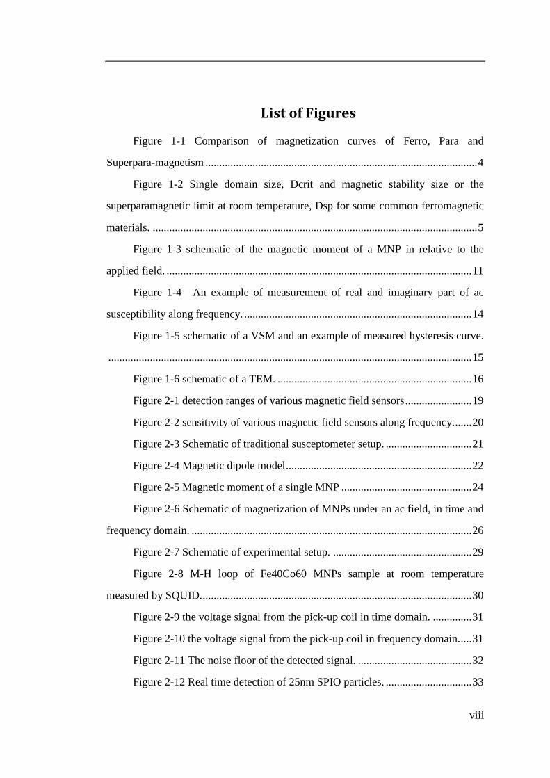
Figure 2-12 Real time detection of 25nm SPIO particles. ............................... 33

ix
Figure 2-13 Signal from pick-up coil is digitized and recorded in time domain.
The applied field (top) contains low frequency 10 Hz and multi-tone high
frequencies (1 kHz, 5 kHz, 10 kHz, 15 kHz, and 20 kHz). The magnetization of
MNPs (bottom) shows the periodic nonlinear response. ........................................... 35
Figure 2-14 Amplitude Spectrum of Magnetization from the MNPs under
multi-tone applied magnetic field. ............................................................................. 36
Figure 2-15 Phase delays of magnetization behind the field at 5 tones are
measured at the same time. ........................................................................................ 37
Figure 2-16 Magnetization curve of Iron Oxide Nanoparticles (SHP35, Ocean
NanoTech, Springdale, AR) in water solution at room temperature measured by
VSM. ......................................................................................................................... 39
Figure 2-17 Hydrodynamic distribution of Iron Oxide Nanoparticles (SHP35,
Ocean NanoTech, Springdale, AR)in water solution at room temperature measured
by DLS. ...................................................................................................................... 39
Figure 2-18 High frequency field is swept from 2 kHz to 20 kHz, and the
phase delay of MNPs is measured at each frequency. A 10 Hz field is applied to
saturate the MNPs with the peak amplitude of 33 Oe, 66 Oe and 99Oe respectively.
................................................................................................................................... 40
Figure 2-19 Signal from pick-up coil is digitized and recorded in time domain.
The applied field (top) contains 10 Hz 99 Oe field and 20 kHz 10 Oe field. The
Brownian magnetization of MNPs (middle) shows periodic nonlinear response. The
phase delay of MNPs (bottom) due to Brownian relaxation also shows periodic
response. ................................................................................................................... 42
Figure 2-20 Phase delay of Néel magnetization behind the 20 kHz field is
recorded during one period of 10 Hz strong field with the amplitude of 33 Oe
(green), 66 Oe (blue) and 99 Oe (red). ...................................................................... 43
Figure 2-21 Left figure: energy barrier under zero offset field; Right figure:
energy barrier under an offset field. ......................................................................... 44

x
Figure 2-22 In-phase and Out-of-phase Amplitude of Brownian relaxation of
SHP35 behind the 20 kHz field is recorded in one period of 10 Hz 99 Oe field. ....... 45
Figure 2-23 Signal from pick-up coil is digitized and recorded in time domain.
The applied field (top) contains 10 Hz 99 Oe field and 20 kHz 10 Oe field. The
magnetization of SHS20 (middle) shows periodic nonlinear response. The phase
delay of SHS20 (bottom) due to Brownian relaxation also shows periodic response.
................................................................................................................................... 45
Figure 2-24 In-phase and Out-of-phase Amplitude of relaxation of SHS20
behind the 10 kHz field is recorded in one period of 10 Hz 99 Oe field. ................... 46
Figure 2-25 MNP phase delay dependence on phase modulation factor n and
amplitude modulation factor m (simulation). ............................................................ 49
Figure 2-26 MNP amplitude dependence on phase modulation factor n and
amplitude modulation factor m (simulation) ............................................................. 49
Figure 3-1 Size distributions of SHP35, IPG35 and IPG35-Ab samples
measured by Dynamic Light Scattering (DLS). ........................................................ 53
Figure 3-2 Experimental plots (dots) of phase delay of mixing-frequency f1+2
f2alongscanning frequencyf1 for three MNP samples in water solution. Debye model
(solid lines) with the superposition of MNPs size distribution shown in Figure 3-1 is
plotted to compare with the experimental data. ......................................................... 54
Figure 3-3 Real time measurement of phase delay of IPG35 in blue and
control sample SMG35 in red, with antibody injection at the 50th
second; .............. 55
Figure 3-4 Phase delay over high frequencies for various MNPs. .................. 57
Figure 3-5 Amplitude over high frequencies for various MNPs. ..................... 58
Figure 3-6 Normalized amplitude over high frequencies for various MNPs. .. 59
Figure 3-7 Normalized amplitude over low frequencies for various MNPs. ... 60
Figure 3-8 MH curve for three MNP samples ................................................. 61
Figure 3-9 Mixing frequency response in time domain ................................... 62
Figure 3-10 Mixing frequency response in frequency domain ........................ 62

xi
Figure 3-11 Calculated probability map of 150 µg SOR15 and 50µg SOR15.
................................................................................................................................... 65
Figure 3-12 Calculated probability map of 100 µg SOR15 and 100µg SOR15.
................................................................................................................................... 66
Figure 3-13 Calculated probability map of 50 µg SOR15 and 150µg SOR15.
................................................................................................................................... 66
Figure 3-14 Calculated probability map of 200 µg SOR15. ............................ 67
Figure 3-15 Linear and Mixing terms along mixing ratio of two MNPs. ........ 67
Figure 3-16 Amplitude of Mixing Frequency along frequency for 5 samples 69
Figure 3-17 Phase delay of high frequency along frequency for 5 samples .... 70
Figure 3-18 Cole-cole plot of complex magnetization amplitude of the 5
samples at different frequencies. ............................................................................... 70
Figure 3-19 Estimation of the amount of two MNPs in 5 samples at different
frequencies. ................................................................................................................ 71
Figure 3-20 MH loop of FeCoAu and FeO30 .................................................. 72
Figure 3-21 Mixing frequencies of FeCoAu along static field. ....................... 74
Figure 3-22 Mixing frequencies of FeO30 along static field. .......................... 74
Figure 3-23 Phase delay over the range of high frequency. ............................ 75
Figure 3-24 Phase delay over the range of low frequency. .............................. 76
Figure 3-25 In-plane MH loop of Fe16N2/Fe thin film. .................................... 77
Figure 3-26 Top figure is the applied field. Middle figure shows the picked-up
voltage from the coil. Bottom figure shows the magnetization calculated from the
voltage signal. ............................................................................................................ 78
Figure 3-27 Zoomed-in plots of Figure 3-26 ................................................... 78
Figure 3-28 MS-1 cell with magnetosomes (bar=1μm). .................................. 79
Figure 3-29 Phase delay along time of magnetosomes in two solution with
different viscosity. ..................................................................................................... 80
Figure 3-30 Size distribution of single magnetosome crystals ........................ 80
Figure 3-31 TEM of clusters of magnetisomes. ............................................... 81

xii
Figure 3-32 Estimated hydrodynamic size distribution of magnetosome
clusters. ...................................................................................................................... 81
Figure 3-33Phase delay over frequencies of magnetosome in different
solutions. .................................................................................................................... 82
Figure 3-34 Phase delay over frequencies of 25nm MNps in two solutions. .. 83
Figure 4-1Thin film structure of GMR grown by Shamrock sputtering .......... 85
Figure 4-2 Patterning of one GMR sensor. Shaded area is active region with
thinner SiO2 protection. ............................................................................................. 85
Figure 4-3 GMR sensor array (16X16) with connectors on the 4 sides .......... 86
Figure 4-4 Schematic of Anderson Loop ......................................................... 87
Figure 4-5 Schematic of Wheatstone brige ...................................................... 88
Figure 4-6 Working principle of mixing frequency method ............................ 90
Figure 4-7 Relationship between mixing terms and sensing current and
excitation field ........................................................................................................... 90
Figure 4-8 Noise floor on a normal linear sensor ............................................ 91
Figure 4-9 An AC resistance response of a GMR sensor in the linear region . 91
Figure 4-10 Noise floor on a normal linear sensor with a 200Hz field ........... 92
Figure 4-11 1st Side tone of GMR in real time by dropping 50nm MACS with
biotin-streptavidin binding ........................................................................................ 92
Figure 4-12 2nd
Side tone of 6 sensors in real time with MACS50 dropped at
17 min. A bias field is supplied. Sensor 21, 23 and 25 are printed with 10ng IL6.
Sensor 20, 22 and 24 are control sensors with BSA blocking. .................................. 93
Figure 4-13 The signal of a sensor array. The red bar shows the control
sensors and the others are active sensors. The first row indicates the reference
sensors under silicon oxide. ....................................................................................... 93
Figure 4-14 Image of 3 printed capture antibody and BSA control on one
sensor ......................................................................................................................... 94
Figure 4-15 Left shows the real time measurement for 5 order concentration of
PAPP-A antigen. Right shows the signal distribution of each concentration. .......... 94

xiii
Figure 4-16 Left shows the real time measurement for 5 order concentration of
PCSK9 antigen. Right shows the signal distribution of each concentration. ............ 95
Figure 4-17 Left shows the real time measurement for 5 order concentration of
ST2 antigen. Right shows the signal distribution of each concentration. ................. 95
Figure 4-18 GMR detection model .................................................................. 96
Figure 4-19 Side tone along DC bias field with different AC field ............... 100
Figure 4-20 Side tone along AC field with different bias DC field. .............. 100
Figure 4-21 Noise of linear sensor in time domain. ....................................... 101
Figure 4-22 Noise of linear sensor in frequency domain. .............................. 101
Figure 4-23 Zoomed in plots of Figure 4-22 ................................................. 102
Figure 4-24 Noise of 40*80 sensor in time domain. ...................................... 102
Figure 4-25 Noise of 40*80 sensor in frequency domain. ............................. 102
Figure 4-26 Zoomed-in plots of Figure 4-25 ................................................. 103
Figure 4-27 Carrier tone drift ......................................................................... 103
Figure 4-28 1st side tone drift ......................................................................... 104
Figure 4-29 2nd
side tone drift ........................................................................ 104
Figure 4-30 Testing condition ........................................................................ 105
Figure 4-31 Top figure shows an input 2Hz signal. Middle figure shows the
output signal from the Wheatstone bridge. Bottom figure shows the output signal
modulated by the fluorescent light. ......................................................................... 106
Figure 4-32 Transfer curve of input-output in dark in 2 Hz .......................... 106
Figure 4-33 Transfer curve of input-output in incandescent light in 2 Hz .... 107
Figure 4-34 Top figure shows an input 10 Hz signal. Middle figure shows the
output signal from the Wheatstone bridge. Bottom figure shows the output signal
modulated by the incandescent light. ...................................................................... 107
Figure 4-35 Transfer curve of input-output in dark in 10 Hz ........................ 108
Figure 4-36 Transfer curve of input-output in incandescent light at 10 Hz ... 108

xiv
Figure 4-37 Top figure shows an input 100 Hz signal. Middle figure shows the
output signal from the Wheatstone bridge. Bottom figure shows the output signal
modulated by the incandescent light. ...................................................................... 109
Figure 4-38 Transfer curve of input-output in dark at 100 Hz ...................... 109
Figure 4-39 Transfer curve of input-output in incandescent light at 100 Hz . 110
Figure 4-40 Schematic of detection system ................................................... 111
Figure 4-41 Schematic of the detection circuit .............................................. 112
Figure 4-42 Closed-loop gain along frequency of OPA827 .......................... 114
Figure 4-43 Input voltage noise density along frequency of OPA827 .......... 114
Figure 4-44 Low frequency output noise in time domain of OPA827 .......... 115
Figure 4-45 Unity-Gain Buffer Configuration ............................................... 115
Figure 4-46 ADG1606 Functional Block Diagram ....................................... 116
Figure 4-47 ADG1606 on Resistance as a Function of VD/VS for Dual Supply
................................................................................................................................. 116
Figure 4-48 ADG1606 Leakage Current as a Function of Temperature for
Dual Supply ............................................................................................................. 117
Figure 4-49 Gain of INA163 along frequency ............................................... 118
Figure 4-50 Noise voltage of INA163 along frequency ................................ 119
Figure 4-51 Noise current of INA163 along frequency ................................. 119
Figure 4-52 Noise floor at DAQ output directly through BNC connector .... 120
Figure 4-53 Noise floor of input signal to PCB measured by a probe ........... 121
Figure 4-54 Noise floor of signal after the voltage follower measured by a
probe ........................................................................................................................ 121
Figure 4-55 Noise floor of signal after the voltage follower measured by a
probe. A low pass filter is enabled before the voltage follower. ............................. 121
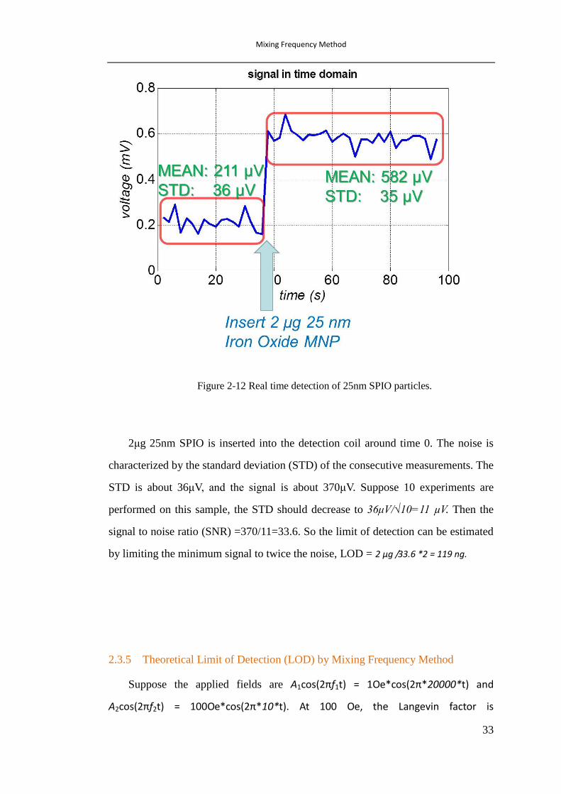
Figure 4-56 Noise floor of signal at the resistor-resistor node in the
Wheatstone bridge ................................................................................................... 122
Figure 4-57 Noise floor of signal at the resistor-sensor node in the Wheatstone
bridge ....................................................................................................................... 122

xv
Figure 4-58 Noise floor of signal after an instrumentation amplifier of 13.5
gain .......................................................................................................................... 122
Figure 4-59 Noise floor of signal after an instrumentation amplifier after a low
pass filter ................................................................................................................. 123
Figure 4-60 Noise floor of 85 mV DC signal provided by a 7.5 V battery and
10 kΩ potentiometer ................................................................................................ 123
Figure 4-61 Left shows the spectrum of a 20 kHz sine signal generated by a
function generator. Right shows the spectrum of a 20 kHz sine signal generated by
DAQ itself. .............................................................................................................. 123
Figure 4-62 A 100 kHz Sin signal sampled by a microcontroller. ................ 124
Figure 4-63 A 100 kHz square wave sampled by a microcontroller. ............ 125
Figure 4-64 Voltage spectrum of Figure 4-63 calculated by FFT module in
DSP core in μC. The peak frequency is 0x00018CB4 = 101556 Hz shows the clock
mismatch between function generator and μC. ....................................................... 125
Figure 4-65 A 2 kHz and a 200 Hz signal are applied to the sensor. The output
shows the mixing frequencies 1.8 kHz and 2.2 kHz. .............................................. 126
Figure 4-66 By modulating 2 kHz input with the output signal in Figure 4-65,
the mixing terms are demodulated in 200 Hz. ......................................................... 127
Figure 4-67 a 3.5 kHz sine wave generated by XR2206 ............................... 127
Figure 6-1 Resonance frequency (left figure) and line width (right figure) of
MNP are dependence on pH of solution (dot represents pH=8; circle represents
pH=6).46
................................................................................................................... 134
Figure 5-2 Structure of a 4-layer PCB ........................................................... 135
Figure 5-3 Coil Design in Sonnet simulation ................................................ 136
Figure 5-4 Magnetic field distribution by HFSS ........................................... 136
Figure 5-5 S-parameter measurement in Sonnet simulation .......................... 137
Figure 5-6 S-parameter measurement in Sonnet simulation.μr is changed to 2
to represent MNPs. .................................................................................................. 137
Figure 5-7 Input impedance measurement in Sonnet simulation. .................. 138

xvi
Figure 5-8 Input impedance measurement in Sonnet simulation. μr is changed
to 2 to represent MNPs. ........................................................................................... 138
Figure 5-9 Coil Design with more turns in Sonnet simulation ...................... 139
Figure 5-10 S-parameter measurement in Sonnet simulation ........................ 139
Figure 5-11 PCB design of various transmission lines .................................. 140
Figure 5-12 S-parameter of TLine1 ............................................................... 140
Figure 5-13 S-parameter of TLine2 ............................................................... 141
Figure 5-14 S-parameter of TLine3 ............................................................... 141
Figure 5-15 S-parameter of TLine4 ............................................................... 142
Figure 5-16 S-parameter of TLine5 ............................................................... 142
Figure 5-17 S-parameter of TLine6 ............................................................... 143

xvii
List of Tables
Table 2-1List of properties of 5 types of MNP ................................................ 23
Table 2-2 List of properties of iron oxide MNPs from Ocean Nanotech. ....... 23
Table 3-1 Amplitude of linear and mixing frequencies of each sample .......... 67
Table 3-2 Composition of 20 nm and 35 nm MNPs in each sample ............... 68
Table 3-3 Estimated results based on amplitude and phase at various
frequencies ................................................................................................................. 71
Table 3-4 Amplitude of linear and mixing frequencies of each sample .......... 73
Table 4-1 GMR sensitivity at different DC bias .............................................. 99

Introduction
1
Chapter 1 Introduction
1.1 Ferromagnetism in a material
Spin and orbital movement of charged particles (electrons, protons) creates
magnetic field. In this study, all the magnetism comes from motion of electrons.
Magnetic field is generated by passing electron current through solenoid conducting
coil (Ampère’s law), and magnetic material’s net moment is from the spin-orbital
coupling of the unpaired 3d electrons.
When a magnetic field H is applied, according to classical physics, there is
an increase of mechanical orbital moment L. With a negative gyromagnetic ratio γ,
the changed magnetic moment μm = L* γ will have an opposite direction to the
applied field. This negatively magnetized phenomenon is called diamagnetism.
Diamagnetism is present in all materials; however it is too weak to be considered in
most experiments and often ignored especially when other strong magnetism is
exhibited. A special property of diamagnetism is its temperature independence.
Some examples of diamagnetic material are copper and water.
On the other hand, the magnetic field also tends to align the local magnetic
dipole to the field’s direction. This phenomenon is called paramagnetism. Quantum
physics limits the orientation of spins to up and down relative to the applied field.
The distribution of the number of up and down spins is regulated by Boltzmann
factors. The total net magnetic moment can be calculated by summarizing the up and
down spins, and turns out to have a negative dependence on the temperature. The
calculated susceptibility is = μm/H = C/T. C is the Curie constant. Material (such
as sodium) with isolated, distinguishable magnetic ions also shows paramagnetic.
This is called Pauli paramagnetism, and is not dependent on temperature.
Another very important magnetism is the ferromagnetism. In ferromagnetic
material, the spins have positive coupling through Heisenberg interaction, which

Introduction
2
means under Curie temperature Tc spontaneous magnetization will happen. The
saturation magnetization Ms also has a negative dependence on the temperature due
to the uncorrelated thermal spin fluctuations. Above Tc, thermal disorder reigns over
the spin-spin coupling, the material shows the paramagnetic property: = μm/H =
C/(T - Tc). This positively coupling mainly exists in 3d electron (transition metal
such as Fe, Co, and Ni) and 4f electron (rare earth material such as Gd and Dy).
Some oxides have the magnetism of superexchange. In these oxides, a 3d
electron of transition metal atom is shared with a 2p orbit of oxygen. Each oxygen
atom has two 2p covalent bonding, and the doubly occupied orbital has two
electrons of opposite spin. Thus the two metal atoms have different spins through the
oxide bonding. The superexchange interaction separate some of the transition metal
atoms from others in term of spin directions, and the two group of atoms with same
spin direction are called site A and site B. If the total magnetic moments of site A
and site B are equal, the material is Antiferromagnetic, and no net moment is
exhibited without applied field; if the two sites have different moment, the material
is Ferrimagnetic. One common superexchange group is iron oxide, including
Antiferromagnetic hematite (α-Fe2O3) and FeO, and Ferromagnetic maghemite
(γ-Fe2O3) and Fe3O4 (magnetite). Susceptibility () of Antiferromagnetic material is
similar to that of Ferromagnet, while Ferrimagnetic 1/ has a nonlinear dependence
on temperature1.
1.2 Superparamagnetism
Magnetic domains exist in bulk ferromagnetic materials to minimize
magnetostatic energy. For very small Magnetic Nano Particles (MNP) compared to
magnetic domain wall in term of size, it costs more energy to create a domain wall
than to support the magnetostatic energy of the single-domain state. When the size
of this single-domain MNP is small enough, even the thermal fluctuation energy

Introduction
3
(KBT) can overcome the anisotropy energy (KUV), and the magnetization can flip
between the two easy axes very fast compared to the measurement time. In this case,
the anisotropy energy can be ignored and zero coercivity is observed. This
phenomenon is like paramagnetic material with giant magnetic moment, thus called
superparamagnetism.
At temperature T, the mean time between two spin flips of a MNP is called
the Néel relaxation time: ,where τ0(attempting time) is a length of
time depending on the characteristic of the material. During one measurement time
τm, the magnetization spin will flip several times if τm »τN, thus the overall measured
magnetization will average to zero. A net magnetization will be measured only if τm
«τN. The state of the nanoparticle (superparamagnetic or blocked) depends on the
measurement time τm and Néel relaxation time τN. When the measurement time τm is
fixed, temperature can affect Néel relaxation time τN, and thus affect the observation
of superparamagnetic state or blocked state.The transition (τm =τN) between these
two states can be determined by the blocking temperature .When
temperature and measurement time are fixed, MNP is considered as
superparamagnetic when . 2Compared with paramagnetism,
superparamagnetism has much higher magnetization. Compared with
ferromagnetism, superparamagnetism has no remanence, thus
superparamagneticMNPs can disperse very well by Van der Waals force in a carrier
fluid and the solution is called ferrofluid.

Introduction
4
Figure 1-1 Comparison of magnetization curves of Ferro, Para and
Superpara-magnetism
SuperparamagneticMNPs have been used for biomedicine such as Magnetic
Resonance Imaging (MRI), cell-, DNA-, protein- separation, RNA fishing, drug
delivery, hyperthermia, and biomarker detection. 3 MNPs are usually ferri or
ferromagnetic. Superparamagnetic iron oxide nanoparticles (SPIO),maghemite
(γFe2O3) and magnetite (Fe3O4) are widely useddue to their relatively easy synthesis
process and establishedbiocompatibility4. However the low saturation magnetization
of SPIO limits their applications. Bulk Fe-Co alloy has the highest saturation
magnetization 240 emu/g at Fe:Co composition ratio of around 60:40, while iron
also has a high saturation magnetization of 220 emu/g. Prof. Wang’s group from
University of Minnesota first proposed the application of bio-compatible
FeCo-Au(Ag). At 20 Oe external field, the moment of an isotropic
Fe0.6Co0.4nanoparticle is 2.4*10-15
emu, which is 17 times larger thanthat of a Fe3O4
nanoparticle and 28 times than that of a γFe2O3nanoparticle. Oxidation usually takes
place for unprotected Fe-Co nanoparticles. Natural oxidation layer (approximately

Introduction
5
1.5nm thick), Au, or SiOx shell through a diffusion control based gas condensation
method can function as a protection layer, at the expense of magnetic moment.
The critical size for superparamagnetic particles depends on the anisotropy
and magnetic moment of the material shown in Figure 1-2Error! Reference source
not found.. As the size of MNPs increases, multi-domains will be formed to
decrease the magnetostatic energy. When the domain wall is at the center of the
MNP, the magnetostatic energy is minimal. When the domain wall is pushed to the
side (maximal magnetization) by an external field, the Zeeman energy is minimal.
However, after the field is removed, the thermal agitation is not strong enough to
create multi-domains by overcoming the exchange energy barrier. Thus net magnetic
moment, also called remanence, is present even without external field. This net
magnetic moment will cause MNPs to form clusters and cannot well disperse in the
solution.
Figure 1-2 Single domain size, Dcrit and magnetic stability size or the
superparamagnetic limit at room temperature, Dsp for some common ferromagnetic
materials.5

Introduction
6
1.3 Magnetic Spin Relaxation
1.3.1 Electron spin dynamics
The dynamics of electron spin include precession and damping, and can be
described by Landau-Lifshitz (LL) equation:
,
where and .
Gilbert later replaced the damping term in the Landau-Lifshitz equation by
one that depends on the time dependence of the magnetic field6:
,
whereγ is gyromagnetic ratio and η is damping constant.
1.3.2 Static magnetization
For superparamagnetic MNPs, in the presence of a DC magnetic field H in z
direction, the magnetic moment of each MNP will follow the Boltzmann
distribution, and the parallel magnetization is:
,
whereL is Langevin function and .
1.3.3 Dynamic magnetization
By the thermal agitation, the MNP will experience Brownian motion and
magnetic spin disorientation. To include the thermal energy, two treatments will be

Introduction
7
introduced here7.
Langevin’s treatment of Brownian motion is listed below:
Where is the friction term, η is the viscosity of the surrounding fluid,
and ‘a’ is the radius of a spherical particle. (t) describes the thermal white noise,
where . D is the diffusion coefficient .
Fokker-Plank treatment considers the magnetization dynamics in term of
drift and diffusion:
Where W is the probability density of orientations of M. J is the current density.
is the magnetization vector. K’ is a constant which determines the extent
of thermal disruption, and its value can be calculated by comparing the solution of
Fokker-Plank equation in DC field to the static magnetization.
Where , and τN is the Néel relaxation time.
1.3.4 Brown’s equation
Suppose the magnetization M only has orientation dependence W(𝜙, ),
where 𝜙 is the azimuthal angle and is the polar angle. The Fokker-Plank
equation can be written as Brown’s equation:

Introduction
8
To solve the Brown’s equation, W is expanded into Legendre harmonics in
spherical coordinates:
are the associated Legendre function.
are the time-dependent functions describing the time evolution of each
spherical harmonic.
describes the evolution of the alignment with the z axis.
describes alignment perpendicular to the z axis.
W Legendre expansion is usually limited to certain number of harmonics in order to
solve the Brown’s equation more conveniently.
1.3.5 Solution to Brown’s equation
To simply the problem, suppose the magnetization has no azimuthal 𝜙
dependence relative to applied field, and energy V only includes Zeeman energy
where anisotropy energy is ignored:
Brown’s equation reduces to:
Replace W with the Legendre expansion, the Legendre coefficients an forms a

Introduction
9
first order equation:
Or in matrix form:
The Laplace transforms of the above equation is an iterative equation:
An can be solved numerically or analytically by truncating the higher order
harmonics.
1.3.6 Néel relaxation time
For small , it is possible to limit the size of matrix to 2*2.
m = 0:
m=1:
The above differential equations can be represented by linear nonhomogeneous
equations with Laplace operator s.
Equating the determinant to zero, we can get the parallel Néel relaxation time:

Introduction
10
Equating the determinant to zero, we can get the perpendicular Néel relaxation
time:
If the uniaxial anisotropy energy is considered, the relaxation time
will have dependence on .
For small σ,
For large σ>1.5, the orientation of magnetization can be treated discrete in the
Wentzel-Kramers-Brillouin-Jeffreys (WKBJ) model, and the relaxation time is:
1.4 AC susceptibility of MNPs
1.4.1 Brownian relaxation
In an AC magnetic field, not only can the magnetic spin follow the field direction,
but also the MNPs can physically rotate by magnetic torque to align to the applied
field. To describe how fast this physical alignment takes, the Brownian relaxation
time τB is introduced:
Tk
D
Tk
V
B
H
B
HB
2
3 3
where η is the viscosity of the carrier or matrix fluid, and VH is the effective

Introduction
11
hydrodynamic volume of MNP, and DH is the effective hydrodynamic diameter.
1.4.2 Total relaxation
Since Néel relaxation and Brownian relaxation occurs simultaneously, the total
relaxation is a combination of these two schemes.
Figure 1-3 schematic of the magnetic moment of a MNP in relative to the applied
field.
Néel relaxation shows that magnetic moment will flip on the two directions of the
easy axis randomly under thermal fluctuation: m(t’)=m × r(t’) × b, where m is the
magnetic moment of a MNP, and r is a stochastic function that has Poison
distribution (±1), and b is the unit magnetization vector. Auto-correlation of r(t’) is
shown by Kenrick in 1929 as8:
Brownian relaxation shows the whole MNP rotate along θ in the viscose surrounding
fluid. Debye in 1929 has shown that auto correlation of cos(θ) is a function of τB:

Introduction
12
So the measured magnetization along the field direction:
Then the auto correlation of measured magnetization is:
From the above expression, the total relaxation time is the geometric mean of Néel
and Brownian relaxation time:
The total relaxation time τ will depend more on the smaller value of τN and τB. So
Néel and Brownian relaxation, which ever will occur faster will dominate the total
relaxation process.
1.4.3 Debye model
Under an AC field H(t) = H0*exp(jωt), at any time instantt0, the field will magnetize
the MNPs, and the magnetization effects will then decay exponentially with the time
constant τ. In other words, magnetization M(t) is not only from the current applied
BN
BN

Introduction
13
field, but also from the previous remanence. So the magnetization can be calculated
by convolving applied field with the decay function.
Where χ0 is the static susceptibility, χ0=Nm2/3kTVμ0, and 𝜙(x) = c(x)/c(0) is the
normalized autocorrelation of the magnetization defined in the previous sector.
Then the AC susceptibility can be expressed in time domain:
The complex susceptibility can be converted in frequency domain using Fourier
Transform, and this is the Debye model used to describe various relaxation
phenomenon including the dielectric dispersion.
As shown above, the AC complex susceptibility can be expressed as the real part
and the imaginary part , or as the amplitude and phase
.

Introduction
14
Figure 1-4 An example of measurement of real and imaginary part of ac susceptibility
along frequency.
1.5 MNPs characterization
1.5.1 VSM
A Vibrating Sample Magnetometer (VSM) is an instrument that measures the static
magnetization of a sample under a range of magnetic field9.

Introduction
15
Figure 1-5 schematic of a VSM and an example of measured hysteresis curve.
A static magnetic field is applied by a Helmholtz coil with soft magnetic core, and
the magnetized sample is vibrated through a vibrating rod. The vibrating frequency
is usually in MHz range and the magnetization of the vibrating sample is picked up
by a pair of pickup coils. The induced voltage in the pickup coil is proportional to
the sample’s magnetic moment, and can be measured by a lock-in amplifier using
the vibration-generating signal as its reference signal. By measuring the
magnetization while sweeping the magnetic field, the hysteresis curve of a material
can be obtained.
1.5.2 SEM and TEM
A scanning electron microscope (SEM) is a type of electron microscope that
produces images of a sample by scanning it with a focused beam of electrons10
. This
instrument has been used to study the surface structure such as the GMR sensor. An
electron beam is formed and focused on a small spot on the sample surface,
producing various signals (the most commonly used is secondary electrons) that can
be detected and that contain information about the sample’ surface topography and

Introduction
16
composition. The electron beam is scanned to generate a whole surface image.
SEM can achieve resolution better than 1 nanometer.
Figure 1-6 schematic of a TEM.
A transmission electron microscopy (TEM) is a microscopy technique whereby a
bean of electron is transmitted through an ultra-thin specimen, interacting with the
specimen as it passes through11
. An image is formed from the interaction of the
electrons transmitted through the specimen. Most recent technology pushes the
detection resolution to below 0.5 Å. TEM has been used to measure the size and the
crystal structure of MNPs.

Introduction
17
1.5.3 DLS
Dynamic light scattering (DLS) is a technique that can be used to determine the size
distribution profile of small particles in solution12
. When light hits small particles,
the light scatters as long as particles are small compared to the wavelength. Since
particles are undergoing Brownian motion in solutions, the scattering intensity will
fluctuate. Brownian motion speed is related to the particles’ hydrodynamic size, so is
the scattering intensity fluctuation. So by observing the time autocorrelation of the
scattering intensity, particles’ overall hydrodynamic size distribution can be
calculated. Compared to TEM, DLS can measure the particles’ organic surface layer
while TEM cannot due to the poor contrast. DLS can estimate the overall particle
size distribution by fitting to the Log-normal function. However, for more complex
distribution like poly-dispersed, Nanosight instrument can track individual particles’
movement and thus can estimate in small scales.
1Robert C. O’Handley, Modern Magnetic Materials: Principles and Applications.
Publication Date: Nov. 26, 1999| ISBN-10: 0471155667| ISBN-13:978-0471155669| Edition: 1
2 Superparamagnetism, (Oct. 22nd, 2012), from
http://en.wikipedia.org/wiki/Superparamagnetism
3 Superparamagnetism, (Oct. 22nd, 2012), from
http://lmis1.epfl.ch/webdav/site/lmis1/shared/Files/Lectures/Nanotechnology%20for%20
engineers/Archives/2004_05/Superparamagnetism.pdf
4Y. Jing, S. He, T. Kline, Y. Xu and J.P. Wang, ‘High-Magnetic-Moment Nanoparticles for
Biomedicine’, 31st Annual International Conference of the IEEE EMBS, Minneapolis, Minnesota,
USA, September 2-6, 2009.
5 K. M. Krishnan, A. B. Pakhomov, Y. Bao, et al.,‘Nanomagnetism and spin electronics: materials,
microstructure and novel properties.’ J Mater Sci 41 (2006) 793-815.
6 Landau-Lifshitz-Gilbert equation, (Oct. 23rd, 2012), from
http://en.wikipedia.org/wiki/Landau%E2%80%93Lifshitz%E2%80%93Gilbert_equation

Introduction
18
7W. T. Coffey, P. J. Gregg, and Y. P. Kalmykov, ‘On the Theory of Debye and Néel Relaxation of
Single Domain Ferromagnetic Particles’, in Advances in Chemical Physics, edited by I. Prigogine
and S. A. Rice (Wiley, New York, 1993), Vol. 83, p. 263
8 B K P Scaife, ‘On the low-field, low-frequency susceptibility of magnetic fluids’, J. Phys.
D: Appl. Phys. 19 (1986) L195-L197
9 Vibrating sample magnetometer, (Oct. 31st, 2012), from
http://en.wikipedia.org/wiki/Vibrating_Sample_Magnetometer
10 Scanning electron microscope, (Oct. 31st, 2012), from
http://en.wikipedia.org/wiki/Scanning_electron_microscope
11 Transmission electron microscope, (Oct. 31st, 2012), from
http://en.wikipedia.org/wiki/Transmission_electron_microscopy
12 Dynamic light scattering, (Oct. 31st, 2012), from
http://en.wikipedia.org/wiki/Dynamic_light_scattering

Mixing Frequency Method
19
Chapter 2 Mixing Frequency Method
2.1 Search-coil Detection
Magnetic nanoparticle detection for biological and medicinal applications
has been achieved by a variety of sensing schemes. The search-coil based sensing
scheme is one of good candidates among them for future point-of-care devices and
systems because of its unique integrated features: relatively high sensitivity at room
temperature13
, dynamic volume detection (non-surface binding), intrinsic superiority
to measure ac magnetic field, functionality as an antenna for wireless information
transmission, application driven properties such as low cost, portability and easy to
use.
Figure 2-1 detection ranges of various magnetic field sensors14
Figure 2-1 summarizes the detection ranges of various magnetic field sensors.
Squid is the most sensitive sensor of static magnetic field. Search coil has a wide

Mixing Frequency Method
20
detection range, and a very high detection limit. For bio-immunoassay, the popular
research topics nowadays are Search-coil, Flux-gate, Giant Magneto-Resistive(GMR)
sensor, and Hall-effect sensor. GMR sensor usually requires the MNPs to be
concentrated on the sensor surface, while search-coil can achieve volume detection.
Figure 2-2 shows each sensor’s sensitivity along frequency. The majority of the
sensors have slightly higher sensitivity at higher frequency due to the nature of 1/f
noise. However, the sensitivity of search coil depends strongly on the frequency,
because the Faraday’s law of induction shows that the voltage signal on the pick-up
coil is proportional to the field frequency. So above 1kHz, search-coil can
out-perform most of the other sensors.
Figure 2-2 sensitivity of various magnetic field sensors along frequency.15

Mixing Frequency Method
21
Figure 2-3 Schematic of traditional susceptometer setup.
In traditional ac magnetic susceptibility measurement such as Physical
Property Measurement System (PPMS)16
, DynoMagSusceptometer17
(shown in
Figure 2-3) and Slit Toroid Device18
, a pair of balanced coils picks up the
magnetization of the sample under an ac magnetic field and a lock-in amplifier or
impedance analyzer is used to detect the complex ac susceptibility. However, this
method suffers from high background fluctuation due to the thermal and mechanical
instability of the coils, as well as the magnetic moment contribution from sample
matrix (e.g. water) and/or container (e.g. plastic tube). Given the small amount of
MNPs sample in the paramagnetic or diamagnetic environment, the background is a
significant portion of the overall signal.
2.2 MNPs magnetic flux in coil (equation and simulation)
The magnetization of a MNP can be treated as dipole model when its external
dipole fields are of interests. A single MNP can generate a net magnetic flux in the
detection coil.

Mixing Frequency Method
22
Figure 2-4 Magnetic dipole model19
In order to calculate the magnetic flux density B, magnetic potential A is
introduced.
If only the observation vector r is perpendicular to the magnetization m,
magnetic field B can be simplified to:
The saturation magnetization for magnetite is Ms = 121.89 emu/cc. And the
saturation magnetic moment ms=Ms * Vol. The magnetic moment of a MNP at
applied field H is:
Where Boltzmann constant is kB = 1.38 * 10-23 J/K = 1.38 * 10-16 erg/K

Mixing Frequency Method
23
Sample m0 (emu=
erg/G) per
particle
m (emu) per
particle (at ±30
Oe)
Concentration Core size by
Langevin
fitting
SHS-10, 10nm 1.0x10⁻¹⁶ 1.9-2.0x10⁻¹⁸ 1mg/mL(Fe)
0.86nmol/mL
7.7 nm
SHS-20, 20nm 5.7x10⁻¹⁶ 1.03-1.13x10⁻¹⁶ 1mg/mL(Fe)
0.11nmol/mL
13.8 nm
SHS-30, 30nm 4.0x10⁻¹⁶ 1.00-1.10x10⁻¹⁶ 1mg/mL(Fe)
0.031nmol/mL
12.3 nm
MACS, 50nm, (12
20nm MNPs)
80.0-82.0x10⁻¹⁶ 22.52-24.7x10⁻¹⁶ 3.14pmol/mL 18.2 nm
Adembeads,
100nm
365-370x10-16 17.01-19.03x10⁻¹
6
1.6pmol/mL
Table 2-1List of properties of 5 types of MNP
For all the iron oxide nanoparticles from Ocean NanoTechnology, their
technical specifications are listed below20
,
Table 2-2 List of properties of iron oxide MNPs from Ocean Nanotech.
From the TEM image, the MNPs have sphere shape for the size below
(including) 30nm. Above 30nm, the shape MNPs is cubic or irregular.

Mixing Frequency Method
24
-100 -50 0 50 100-3
-2
-1
0
1
2
3x 10
-16
Field (Oe)
Magnetization p
er
MN
P (
em
u)
SHS-10
SHS-20
SHS-30
Figure 2-5 Magnetic moment of a single MNP
At 100 Oe, the magnetic moment of a single 30nm MNP is about m= 1.2e-16
emu = 1.2e-19 Am2.
Suppose the detection coil has a radius of R=0.01m, the total magnetic flux
generated by a single MNP can be calculated as:
Suppose the applied field is 100 Oe 100 Hz pure sin wave, and the detection
coil has 500 turns. According to Faraday’s law of induction, the picked-up voltage
is:

Mixing Frequency Method
25
For our DAQ NI USB-6281, the minimum voltage range sensitivity is about 0.8
μV, so the minimum amount of MNPs detectable is:
0.8e-6/1.3e-16 = 3.4e10.
The SHS30 concentration is 0.31nmol/mL=1.87e14 MNPs/mL, and that makes
the minimum detection limit to be 3.4e10/1.87e14=1.8e-4mL=180nL, that is 180ng
Fe.
The more accurate to calculate the detection limit should consider the MNPs
magnetic noise, magnetic field noise, cancelation effect of magnetization in the
differentially wound detection coil pair, thermal noise of detection coil, noise figure
of instrumentation amplifier, and tone measurement method.
2.3 Mixing Frequency Method
2.3.1 Introduction to the Mixing Frequency Method

Mixing Frequency Method
26
To differentiate the MNPs from the background signal, the magnetization of
them needs to be compared. MNPs are superparamagnetic, and part of the
background signal is from paramagnetic material. As shown in Figure 1-1
superparamagnetic MNPs saturate much easier than paramagnetic material. Based
on this property, when an ac magnetic field is applied as shown in Figure 2-6, the
MNPs will be driven into saturation region while paramagnetic background is still in
linear region. The nonlinear magnetization will generate higher harmonic signals on
the pick-up coil. These higher harmonics are very specific to the MNPs, thus can be
used for MNPs detection. Noticing that due to the rotational symmetry, the
magnetization only contains the odd higher harmonics.
In order to achieve highly sensitive detection, the field strength needs to be big
enough to generate strong signal of harmonics. On the other hand, Faraday’s law of
induction requires high frequency to generate big voltage on the pick-up coil.
Figure 2-6 Schematic of magnetization of MNPs under an ac field, in time and frequency
domain.

Mixing Frequency Method
27
However, the power amplifier that drives the excitation coils can only output a
certain amount of power, and the power consumption is proportional to the current
and frequency. Big field strength and high field frequency cannot be achieved at the
same time. In order to solve this dilemma, a mixing-frequency method21
has been
used to detect the nonlinear magnetization of MNPs per testing sample by measuring
the amplitude of the mixing frequency signals and thereby avoid the high noise at
the fundamental frequencies22,23
. A magnetic field with low frequency (e.g. f2=10
Hz) and large amplitude drives the MNPs into their nonlinear saturation region
periodically.Another magnetic field with higher frequency (e.g. f1=20 kHz), and
with a relatively small amplitude due to the inductance of excitation coil, is used to
transfer the nonlinearity into the mixing frequency signals, such as f1 + 2 f2 (20.02
kHz). In this higher frequency region, the detection coil has higher output voltage
amplitude, and the measurement system has lower 1/f noise, thus the
mixing-frequency method can greatly improve the signal-to-noise ratio.
2.3.2 Theory of the Mixing Frequency Method
Superparamgnetic nanoparticles with small sizes are typically being used for
biological applications to avoid the aggregation as well as any negative influence
without external field. Its magnetization curve can be expressed as:
)( 00
Tk
HmLMM
B
S
(1),
WhereMS is the saturation magnetization,m0 is the magnetic moment of a
singleparticle, µ0is the magnetic permeability of vacuum, His the applied field, kB is
the Boltzmann constant, T is the absolute temperature, and Lis the Langevin
function.
Two sinusoidal magnetic fields are applied simultaneously: one with low
amplitudeA1, high frequencyf1, written asA1cos(2πf1t); the other with high
amplitudeA2, low frequencyf2, written asA2cos(2πf2t). The sum of these two fields (H)
is transferred to magnetization (M) byLangevin function. Taylor Expansion near

Mixing Frequency Method
28
zero magnetization shows that, besides the linear response, the major mixing
components are as the following22:
])2(2cos[4
3)]2cos()2cos([ 21
2
21
3
2211 tffAAtfAtfA
(2)
There are two relaxation mechanisms for MNPs. The physical rotation of
particle in the viscous medium is called Brownian relaxation, and magnetic dipole
flipping inside a stationary particle is calledNéel relaxation. Brownian
relaxationdepends on an effective hydrodynamic volume.Néel relaxation depends on
magnetic volume. The total relaxation process is a parallel model of these two
relaxation schemes, but Brownian relaxation dominates when MNP’s diameter is
large, e.g. iron oxide MNP’s diameter is larger than 20 nm24
:
Tk
V
B
HBtotal
3 (3),
where η is the viscosity of the carrier or matrix fluid, and VH is the effective
hydrodynamic volume of MNP.
When the frequency of ac applied field is low, the particles’ magnetization can
follow the excitation field tightly, and the susceptibility χ is a real number.Asthe
excitation frequency increases, the particles’ magnetization cannot follow the
excitation field, and the relaxation processes introduce a phase in the complex ac
susceptibility. The relationship between relaxation time τ and phase φ of ac
susceptibility can be calculated using Debye model25
.
jj ee
j
)(tan
2
001
)(11)( (4),
whereχ0 is the static susceptibility and ω is the angular frequency. Assuming the
particles’ magnetization has a phase delayφ1to the high frequency field and a phase
delayφ2 to the low frequency field, the mixing-frequency component of
magnetization becomes:
]2)2(2cos[4
3)]2cos()2cos([ 2121
2
21
3
222111 tffAAtfAtfA
(5)
The total relaxation phaseφ1+2φ2 can therefore be determined by measuring the

Mixing Frequency Method
29
phase of the mixing frequency at f1+2f2.If one frequency (e.g. f2) is fixed, and the
other frequency (e.g. f1) is swept, the relaxation phase φ1+2φ2alongf1 will show the
relationship between φ1 andf1. Either one of f1 and f2 can be swept depending on
whether high frequency region or low frequency region is of interest.
2.3.3 Experimental setup
Our search-coil based Susceptometry setup includes two excitation coils that
generate10 Hz ac field with 100 Oe amplitudeand20 kHz ac field with 10 Oe
amplitude, respectively. One pair of pick up coils with differentially wounded 500
rounds is installed. An instrumentation amplifier connected to a digital acquisition
card (DAQ) is used for the signal amplification. LabVIEW program for the
instrument control and Matlab program for signal processing are installed in the
computer for controlling the whole setup.
Figure 2-7 Schematic of experimental setup.

Mixing Frequency Method
30
2.3.4 MNPs detection
Fe40Co60 MNPs are used for the demonstration of MNPs detections. In the room
temperature, the SQUID measurement in Figure 2-8 shows that the sample is
superparamagnetic. By applying two magnetic fields, the magnetization responds
not only to these two frequencies respectively in Figure 2-9, but also generate mixing
frequencies at f1±2f2as shown in Figure 2-10.
Figure 2-8 M-H loop of Fe40Co60 MNPs sample at room temperature measured by
SQUID.

Mixing Frequency Method
31
0.008 0.01 0.012 0.014 0.016 0.018
-0.06
-0.04
-0.02
0
0.02
0.04
0.06
time (s)
voltage (
V)
Figure 2-9 the voltage signal from the pick-up coil in time domain.
1500 2000 2500 30000
0.05
0.1
0.15
0.2
0.25
0.3
frequency (Hz)
voltage (
mV
) f1 + 2f
2
f1 - 2f
2
Figure 2-10 the voltage signal from the pick-up coil in frequency domain.

Mixing Frequency Method
32
0 10 20 30 40 5010
-3
10-2
10-1
frequency (kHz)
vo
lta
ge
(m
V)
noise floor (log scale)
Figure 2-11 The noise floor of the detected signal.
The voltage signal after being amplified with a gain of 10000 is fed to a DAQ.
The noise floor as shown in Figure 2-11 has a typical 1/f noise floor. This again
explains why high frequency detection is required. To test the limit of detection,
25nm SPIO nanoparticles are used.
Mixing Frequency Method
33
Figure 2-12 Real time detection of 25nm SPIO particles.
2μg 25nm SPIO is inserted into the detection coil around time 0. The noise is
characterized by the standard deviation (STD) of the consecutive measurements. The
STD is about 36μV, and the signal is about 370μV. Suppose 10 experiments are
performed on this sample, the STD should decrease to 36μV/√10=11 µV. Then the
signal to noise ratio (SNR) =370/11=33.6. So the limit of detection can be estimated
by limiting the minimum signal to twice the noise, LOD = 2 µg /33.6 *2 = 119 ng.
2.3.5 Theoretical Limit of Detection (LOD) by Mixing Frequency Method
Suppose the applied fields are A1cos(2πf1t) = 1Oe*cos(2π*20000*t) and
A2cos(2πf2t) = 100Oe*cos(2π*10*t). At 100 Oe, the Langevin factor is

Mixing Frequency Method
34
9662.0009662.000 HTk
Hm
B
. Then the mixing terms will be
...])2(2cos[4
...5.1])2(2cos[45.1])(2cos[32.0])(2cos[0032.0...
...])2(2cos[85.1])2(2cos[85.1
])(2cos[00322.0])(2cos[00322.0...
...])2(2cos[)(60
1])2(2cos[)(
60
1
])(2cos[3
])(2cos[3
....
...)(45
1
3
)(
22
23002300
0000
330000
00
tff
etffetftfM
tffAAetffAAe
tfAtfAM
tffAATk
mtffAA
Tk
m
tfATk
mtfA
Tk
mM
HTk
mMH
Tk
mM
Tk
HmLMM
LH
LHLHS
LHLHLHLH
LLHHS
LHLH
B
LHLH
B
LL
B
HH
B
S
B
S
B
S
B
S
The above equation shows that the magnetization of mixing terms to that of low
frequency (100Hz) field is 1.5e-4:0.32=1:2133. Section 2.2 calculates 180ng Fe is
the LOD for the low frequency. Considering the 2133:1 magnetization ratio and
100:20000 frequency ratio, the LOD for the mixing frequency
is180ng*2133/200=1.92μg.
2.4 Multi-tone Mixing-frequency method
Real-time magnetization of SMG30 samples can be digitized by DAQ shown
in Figure 2-13. The magnetization shows nonlinear responses (bottom figure) to the
applied fields (top figure). When the 10 Hz low frequency strong field reaches

Mixing Frequency Method
35
maximum absolute amplitude (e.g. 0.125s, 0.175s, 0.225s, 0.275s), the MNPs show
smaller magnetization response to the high frequencies due to the saturation of the
nonlinear susceptibility. According to Faraday’s law of induction, the electrical
potential from the pick-up coil is proportional to the frequency of the magnetization.
Although MNPs response mainly to 10Hz field, the higher frequency responses of
magnetization are picked up by the coil. The high frequency picked-up voltage
signal is modulated by the 10Hz field, and mixing frequencies are generated.
0.1 0.15 0.2 0.25 0.3-200
-100
0
100
200
Fie
ld (
Oe
)
Applied Field
0.1 0.15 0.2 0.25 0.3-4
-2
0
2
4
Time (s)
Vo
lta
ge
(m
V)
Magnetization of MNPs from Pick-up Coil
Figure 2-13 Signal from pick-up coil is digitized and recorded in time domain. The
applied field (top) contains low frequency 10 Hz and multi-tone high frequencies (1
kHz, 5 kHz, 10 kHz, 15 kHz, and 20 kHz). The magnetization of MNPs (bottom)
shows the periodic nonlinear response.
The number of field tones is limited by the driving capacity of power
amplifier. Multiple tones will create higher PAPR (Peak to Average Power Ratio),
and so the power amplifier will work in a low efficiency and high distortion region.
To address this issue, low PAPR wave with multiple tones, such as square wave, can
be used to probe the rich frequency responses of MNPs.

Mixing Frequency Method
36
Figure 2-14 Amplitude Spectrum of Magnetization from the MNPs under
multi-tone applied magnetic field.
Figure 2-14 gives a frequency overview of the magnetization from MNPs in
the multi-tone field. Each tone generates multiple mixing frequencies. Using a
Quadrature detection method, the phase of mixing-frequencies and the tone
frequencies can be estimated. The amplitude of the mixing frequencies around 5 kHz
is about 50 µV while the noise floor is about 1 µV, and this pushes the limit of
detection to 0.2 µg/mL Fe or 6.2 pM concentration without any improvement by
averaging.

Mixing Frequency Method
37
The phase delay at five tones is plotted with red dots in Figure 2-15. Since the
measurement of phase delays is an overall performance of MNPs with different
hydrodynamic sizes, the size distribution can be estimated using Least Mean Square
(LMS) method. Singular value decomposition (SVD) is one of the LMS methods
that enable efficient and accurate estimation of the unknown variables (size
distribution) from equations (phase delay)32
. However SVD is not accurate when the
number for phase delay measurements is less than the number of size distribution
points, it is not applicable for the multi-tone method since the tone numbers are very
limited. Fortunately most MNPs has a size distribution of Log-normal function24,
2
20
2
2
)/(ln
2
1)(
hh dd
h
h ed
df
where dh0 and β are the mean and the standard deviation of hydrodynamic sizes.
Under this assumption, there are only two unknown variables dh0 and β that needs to
be estimated from the measured phase delay φ at different frequencies ωi. The fitting
0 5 10 15 20 250
5
10
15
20
25
30
35
40
Frequency (kHz)
Ph
ase
de
lay (
o)
Debye model
Experiment
Figure 2-15 Phase delays of magnetization behind the field at 5 tones are measured
at the same time.

Mixing Frequency Method
38
system shown below can be modeled using Matlab function ffun=fittype(expr), with
expr representing the model:
iii
hiij
df
1)()( 0
Then, the function fit(xdata, ydata, ffun) uses this model to get a reasonable
estimation of dh0= 36.5 nm and β= 0.083. Based on this estimated size distribution,
phase delay over frequency is plotted in blue line in Figure 2-15. The experimental
data and the estimation model matches well.
The multi-tone method uses one pick-up coil to measure different
frequencies simultaneously and thus enables a very robust correlation of
measurements at different frequencies. This is in contrast to the frequency sweeping
method, which may be subject to system-level drift. Also, the multi-tone method is
time efficient, so the size distribution of MNPs can be measured consecutively in
real time, which is critical for many applications such as dynamic detection of
binding kinetics and interaction affinities between biomolecules.
2.5 Relaxation modulation by field amplitude
2.5.1 Brownian relaxation modulation
A 10 µL SHP35 sample with a concentration of 5 mg/mL Fe is used for the
test. SHP35 has 35nm Magnetite core and is coated with monolayer oleic acid and
monolayer amphiphilic polymer which added a few nanometers to its hydrodynamic
size. As shown in Figure 2-17 measured by a Dynamic Light Scattering (DLS)
instrument, the sample is well dispersed in water solution and has a narrow
distribution of hydrodynamic size. Under ac magnetic field, due to the large size of
the magnetic core, Brownian relaxation will dominate, and MNPs will physically
rotate in the solution.

Mixing Frequency Method
39
Figure 2-16 Magnetization curve of Iron Oxide Nanoparticles (SHP35, Ocean
NanoTech, Springdale, AR) in water solution at room temperature measured by
VSM.
Figure 2-17 Hydrodynamic distribution of Iron Oxide Nanoparticles (SHP35,
Ocean NanoTech, Springdale, AR)in water solution at room temperature measured
by DLS.

Mixing Frequency Method
40
A 10 Hz 99 Oe magnetic field is applied to saturate the SHP35 samples
periodically, and a high frequency field is applied to generate mixing-frequency
signals. The high frequency field is swept from 2 kHz to 20 kHz, and the measured
phase delay φH to the high frequency is plotted in the red line in Figure 2-18. Phase
delay φL to the low frequency is a small constant number and is not shown here. An
interesting finding is that when decreasing the amplitude of 10 Hz field to 66 Oe and
further to 33 Oe, the phase delay φH of MNPs increases. Similar results have been
reported and discussed in other studies 26,27
.
Figure 2-18 High frequency field is swept from 2 kHz to 20 kHz, and the phase
delay of MNPs is measured at each frequency. A 10 Hz field is applied to saturate
the MNPs with the peak amplitude of 33 Oe, 66 Oe and 99Oe respectively.
To explain the field amplitude dependence of the phase delay, magnetization
of SHP35 samples is digitized by a Digital AcQuisition card (DAQ) in the time
domain as shown in Figure 2-19. The magnetization shows nonlinear responses

Mixing Frequency Method
41
(middle figure) to the applied fields (top figure). When the 10 Hz low frequency
strong field reaches the maximum absolute amplitude (e.g. at 0.025 s, 0.075 s), the
MNPs show smaller magnetization response to the high frequencies due to the
saturation of the nonlinear susceptibility. The amplitude of the high frequency
response can be interpreted as the first derivative of the MH curve28
. According to
the Faraday’s law of induction, the electrical potential from the pick-up coil is
proportional to the frequency of the magnetization. Although MNPs respond mainly
to 10 Hz field, the higher frequency responses of magnetization picked up by the
coil are much stronger. The high frequency picked-up voltage signal is modulated
by the 10 Hz field, and mixing-frequencies are generated. The bottom figure of Fig.
4 shows that not only is amplitude of magnetization modulated by the 10 Hz field,
but the phase of magnetization is also modulated. The 10 Hz field changes much
slower than 20 kHz field, and thus can be viewed as a quasi-static field. During each
period of the 20 kHz field, the phase of the magnetization can be measured using a
Quadrature detection method. When this quasi-static 10 Hz field reaches zero
amplitude, MNPs have the maximum phase delay to the 20 kHz field. This indicates
that SHP35 has smaller Brownian relaxation time in a bigger applied offset magnetic
field. The phase variation means that the measured φH depends on the field
amplitude and is related to the overall phase delay in one period of low frequency.

Mixing Frequency Method
42
Figure 2-19 Signal from pick-up coil is digitized and recorded in time domain. The
applied field (top) contains 10 Hz 99 Oe field and 20 kHz 10 Oe field. The Brownian
magnetization of MNPs (middle) shows periodic nonlinear response. The phase
delay of MNPs (bottom) due to Brownian relaxation also shows periodic response.

Mixing Frequency Method
43
2.5.2 Néel relaxation modulation
The same phenomenon is observed for Néel relaxation in superparamagnetic
MNPs with iron oxide core of 12 nm, on average, plus a fatty acid coating and a
polymer coating. These MNPs has been tested for the purpose of hyperthermia, and
they generate the same amount of heat in liquid solution and in agarose gel, which
indicates that Néel relaxation dominates the magnetization dynamics. Figure 2-20
shows the phase delay of Néel magnetization behind the 20 kHz field during one
period of 10Hz strong field with the amplitude of 33Oe (green), 66Oe (blue) and
99Oe (red). The phase of 20 kHz magnetization is traced in real time using
Quadrature detection. At zero quasi-static field, phase delay reaches maximum, and
drops as the field amplitude increases.
Figure 2-20 Phase delay of Néel magnetization behind the 20 kHz field is recorded
during one period of 10 Hz strong field with the amplitude of 33 Oe (green), 66 Oe (blue)
and 99 Oe (red).

Mixing Frequency Method
44
Néel relaxation model in Figure 2-21 intuitively shows a simple treatment that
the ln(τN) is positively correlated with the energy barrier. When an offset field H0 is
applied, the energy barrier decreases (by M H0), as do τN and φ = tan-1
(ωτN). A more
theoretical treatment of relaxation time can be found in Ref. [4]. In the case of small
ξ, τN≈ τN0(1-2 ξ 2/15), where τN0 is the Néel relaxation time in zero static field; in the
case of large ξ, τN≈ τN0/ ξ29
. Since the MNPs used for Néel relaxation measurement
form clusters, the effective field energy becomes much bigger, and the measurement
results in Figure 2-20 agrees with the second case where ξ is comparably large.
Figure 2-21 Left figure: energy barrier under zero offset field; Right figure: energy
barrier under an offset field.

Mixing Frequency Method
45
Figure 2-22 In-phase and Out-of-phase Amplitude of Brownian relaxation of SHP35
behind the 20 kHz field is recorded in one period of 10 Hz 99 Oe field.
0 0.02 0.04 0.06 0.08 0.1-200
0
200
Fie
ld (
Oe)
Applied Field
0 0.02 0.04 0.06 0.08 0.10
0.1
0.2
Voltage (
mV
)
Magnetization Amplitude of 20nm MNPs from Pick-up Coil
0 0.02 0.04 0.06 0.08 0.10
5
10
Time (s)
Phase D
ela
y (
o) Phase Delay of 20nm MNPs
Figure 2-23 Signal from pick-up coil is digitized and recorded in time domain.
The applied field (top) contains 10 Hz 99 Oe field and 20 kHz 10 Oe field. The
magnetization of SHS20 (middle) shows a periodic nonlinear response. The phase
delay of SHS20 (bottom) due to Brownian relaxation also shows periodic response.

Mixing Frequency Method
46
0 0.02 0.04 0.06 0.08 0.10
0.01
0.02
0.03
0.04
0.05
0.06
0.07
Time (s)
Voltage (
mV
)In-phase and Out-of-phase Amplitude of SHS20
in-phase amplitude
out-of-phase amplitude
Figure 2-24 In-phase and Out-of-phase Amplitude of relaxation of SHS20 behind the
10 kHz field is recorded in one period of 10 Hz 99 Oe field.
Figure 2-23 and Figure 2-24 show the magnetization response from SHS20.
For this MNPs, the phase is not modulated by the low frequency field, only the
amplitude is modulated.
The discussion above shows that both the amplitude and the phase of the
MNPs are modulated by a frequency 2fL. Both the modulations lead to a mixing
frequency fH ± 2fL. Figure 2-22 shows that in-phase and out-of-phase amplitudes of
SHP35 are modulated by a frequency 2fL. The out-of-phase amplitude is affected
more by the quasi-static field. All these factors increase the complexity in
susceptibility modeling. However, this study improves the previous understanding of
the mixing-frequencies from the MNPs, and can help to tailor MNPs to specific
application, such as MPI where gradient static field is used to determine the location
of MNPs. Also, this study provides an experimental method to design new detection

Mixing Frequency Method
47
instruments. For example, if SHP35 MNPs are used as detection probes, the
out-of-phase detection will be more effective, because it not only avoids the
interference from the high frequency field but also is heavily modulated by the low
frequency field.
2.5.3 Simulation of relaxation modulation
Both the amplitude and phase of the high frequency fH magnetization are
modulated by the low frequency fL field, and both modulations contribute to the
amplitude and phase of the mixing frequencies fH ± 2fL. How the modulations affect
the amplitude and phase is complicated. Below analytical and simulation results are
shown.
Under two magnetic fields: H = AH cos(2πfHt) + AL cos(2πfLt), assume
magnetization of MNP has phase delay φHto the high frequency field, and assume
we can ignore the small phase delay φL to the low frequency field. The amplitude
and phase of the magnetization at fH are modulated by the low frequency field with
factors m and n. So the magnetization can be written as:
The modulation factors and have a
fundamental frequency of 2fL.When the phase of a sinusoidal wave cos(ωcn) is
modulated by another sinusoidal wave cos(ωmn), the signal can be decomposed of
mixing frequencies terms30
.

Mixing Frequency Method
48
Where Jk(a) are the Bessel functions of the first kind, ωc corresponds to fH and ωm
corresponds to 2fL. The mixing frequency fH ± 2kfL should have a phase of kπ/2.
However, the amplitude modulation will also generate mixing frequency fH ± 2kfL.
The final mixing term fH ± 2fL will be from numerous combinations of phase
modulation and amplitude modulation. The analytical solution will be so
complicated that numerical simulation is used to help guide the study.
In the Matlab simulation, we try to simulate the situation in Figure 2-19 wherefH
=20000, fL =10, and 𝜑H =60°. Now modulation factors m and n are swept to
study the phase of fH + 2fL.In Figure 2-25, it showsMNP phase delay dependence on
phase modulation factor n and amplitude modulation factor m. When amplitude
modulation factor m is 0, only the phase modulation plays a role in generating the
mixing frequencies fH ± 2fL. However, the phase modulation decreases the phase
delay 𝜑H.When the phase modulation n is fixed, the amplitude modulation m will
also decrease the phase delay 𝜑H. When the amplitude modulation m is fixed, the
phase modulation n will increase thephase delay 𝜑H. In Figure 2-26, both amplitude
modulation factor m and phase modulation n will contribute the amplitudes of the
mixing frequencies. However, the relationship between phase/amplitude and
modulation factors m/n is too complicated to generalize an exact rule.

Mixing Frequency Method
49
0 5 10 15 2040
50
60
70
80
90
100
110
120
130
no (phase modulation factor)
MN
P P
hase D
ela
y o
m=0
m=0.1
m=0.2
m=0.3
m=0.4
m=0.5
Figure 2-25 MNP phase delay dependence on phase modulation factor n and
amplitude modulation factor m (simulation).
0 5 10 15 200
0.02
0.04
0.06
0.08
0.1
0.12
no (phase modulation factor)
MN
P a
mplit
ude
m=0
m=0.1
m=0.2
m=0.3
m=0.4
m=0.5
Figure 2-26 MNP amplitude dependence on phase modulation factor n and
amplitude modulation factor m (simulation)

Mixing Frequency Method
50
13 J. Lenz, IEEE Proceedings, 78, 973, (1990)
14 Caruso, Michael J; Tamara Bratland; Carl H Smith, PhD; and Robert Schneider, “A
New Perspective on Magnetic Field Sensing,” Honeywell Inc, May 1998,
www.ssec.honeywell.com/ magnetic/datasheets/new_pers.pdf
15http://www.boulder.nist.govdiv81881803MagneticDevicesandNanoStructuresindex.ht
ml
16 Quantum Design, San Diego, CA, ‘http://www.qdusa.com/products/ppms.html’ 17Imego Institute, Göteborg, SWEDEN, ‘http://www.imego.com/Products/dynomag/index.aspx’
18P.C. Fannin, B.K.P. Scaife, J. Magn.Magn.Mater.72, 95 (1988)
19 Magnetic dipole, 11/9/2012, from ‘http://en.wikipedia.org/wiki/Magnetic_dipole’
20 http://www.oceannanotech.com/upload/090604131348592520yef2g1.pdf
21 T.L. Paoli and J.F. Svacek, Rev. Sci. instrum., 47, 9 (1976) 22
Petr I. Nikitin, Petr M. Vetoshko, and Tatiana I. Ksenevich, J. Magn. Magn.Mater.311, 445 (2007) 23
Hans-Joachim Krause, Norbert Wolters, Yi Zhang, Andreas Offenhausser, Peter Miethe, Martin H.F.
Meyer, Markus Hartmann, and Michael Keusgen, J. Magn. Magn.Mater.311, 436 (2007) 24 R.E. Rosensweig, J. Magn. Magn.Mater.252, 370 (2002) 25
M.I. Shliomis, Yu.L. Raikher, IEEE Trans. Magn. MAG-16, 237 (1980)
26J Dieckhoff, M. Schilling, and F. Ludwig, “Fluxgate based detection of magnetic nanoparticle
dynamics in a rotating magnetic field.”Appl. Phys. Lett., vol. 99, p. 112501, 2011
27 T. Yoshida, K. Enpuku, J. Dieckhoff, M. Schilling, and F. Ludwig, “Magnetic fluid dynamics in a
rotating magnetic field” J. Appl. Phys., vol. 111, pp. 053901, 2012
28 T. L. Paoli and J. F. Svacek, “Derivative measurement by frequency mixing,” Rev. Sci. Instrum.,
vol. 47, p. 1016, 1976
29 W. T. Coffey, P. J. Cregg, and Y. P. Kalmykov, “On the theory of Debye and Néel relaxation of
single domain ferromagnetic particles,” Advances in Chemical Physics, vol. 83, p. 263, 1993
30 http://crca.ucsd.edu/~msp/techniques/v0.11/book-html/node86.html

Application of Mixing Frequency Method
51
Chapter 3 Application of Mixing Frequency Method
1. 1 Brownian Relaxation Measurement
3.1.1 Brownian Relaxation Measurement by Mixing Frequency Method
Under two magnetic fields: H = AH cos(2πfHt) + AL cos(2πfLt), the sum of these two
fields (H) is transferred to magnetization (M) according to the Langevin function.
Assuming the particles’ magnetization has a phase delay φH to the high frequency field
and a phase delay φL to the low frequency field, Taylor Expansion near zero
magnetization shows that, besides the linear response, the major mixing components with
no DC field are as the following31
:
According to Faraday’s Law of Induction, the voltage signal from the pick-up coil
has a 90° phase shift from the magnetization of MNPs.
...]2)2(2cos[)(60
1
]2)2(2cos[)(60
1...
...)(45
1
3
)(
2300
2300
330000
00
LHLHLH
B
LHLHLH
B
B
S
B
S
B
S
tffAATk
m
tffAATk
m
HTk
mMH
Tk
mM
Tk
HmLMM
...]2
32)2(2cos[)2()(
30
]2
32)2(2cos[)2()(
30...
2300
2300
LHLHLHLH
B
LHLHLHLH
B
tffffAATk
m
tffffAATk
m
dt
dMV

Application of Mixing Frequency Method
52
The relaxation phase φH and φL can therefore be determined by measuring the
phase of the mixing frequency at f1± 2f2.
3.1.2 Real-time Brownian Relaxation Measurement
Three commercial iron oxide MNPs samples (Ocean Nanotech, Springdale, AR) are
used for Brownian relaxation study: SHP35 (MNPs with 35 nm core size, 4 nm oleic acid
and amphiphilic polymer coating, 0.1 mL, 5 mg/mL in H2O-Carboxylic Acid solution),
IPG35 (SHP35 conjugated with around 10 nm protein G layer, 0.1 mL, 1 mg/mL), and
IPG35-Ab (IPG35 conjugated with around 10 nm Goat anti-Human IgG (an antibody
isotype of mammals) HRP with ratio 1:100, 0.1 mL, 1 mg/mL). Particle size distributions
are measured by a Dynamic Light Scattering (DLS) instrument (‘90 Plus Particle Sizer’,
Brookhaven Instruments Corp., Holtsville, NY) and are shown in the Figure 3-1. The DLS
measurement results are consistent with the data provided by Ocean Nanotech. All the
three samples are from the same batch of 35 nm iron oxide MNP core, so the wide
hydrodynamic size distribution of IPG35-Ab shows that IPG35 binds with antibodies in a
range of binding affinity. This is also confirmed by an independent gel electropherosis
measurement (results not shown here).
4
2
2121
2121
22
22
ffff
L
ffff
H

Application of Mixing Frequency Method
53
Figure 3-1 Size distributions of SHP35, IPG35 and IPG35-Ab samples measured by
Dynamic Light Scattering (DLS).
We measured the MNPs’ phase delay of these three samples under ac fields. Phase
delay of the mixing-frequency signal is measured by scanning the frequency of f1 up to
10 kHz. The results of 10 times average are shown in Figure 3-2. To prevent any
temperature drift due to joule heating of the coil, tone bursts are applied rather than
continuous ac field. The experimental results are fitted by the Debye model in Eq. (4).
Since the particles are not monodispersed, the total susceptibility comes from the
contributions of all MNPs with various sizes. As shown in the Figure 3-2, Debye model
with the superposition of MNPs’ hydrodynamic size distribution32
is a good fit in our
case, although it is argued that Debye model is only valid for small-amplitude (<1
kA/m)33
low-frequency34
applied ac field and a high frequency susceptibility χ∞ is
needed for the Debye fitting33
.

Application of Mixing Frequency Method
54
Figure 3-2 Experimental plots (dots) of phase delay of mixing-frequency f1+2
f2alongscanning frequencyf1 for three MNP samples in water solution. Debye model
(solid lines) with the superposition of MNPs size distribution shown in Figure 3-1 is
plotted to compare with the experimental data.

Application of Mixing Frequency Method
55
The binding process of the antibody to protein coated MNPs solution is detected by
monitoring real time relaxation. Instead of the time-consuming whole frequency scan, the
frequencyf1 is fixed at a 4 kHz due to the high signal-to-noise ratio around this frequency
region (detection coil is not sensitive in lower frequency region while MNP has low ac
susceptibility in higher frequency region). 0.05 mL antibody (Goat anti-Human IgG HRP
conjugated, 5 mg/mL) is dropped onto 0.1 mL IPG35 sample. The antibody sample will
then diffuse slowly into IPG35 solution, and gradually bind to protein G on the surface of
MNPs, until protein G binding sites on MNPs are saturated with antibody and has the
same hydrodynamic size distribution as the standard IPG35-Ab sample prepared by the
Ocean NanoTech. On the surface of IPG35 MNPs where protein G is not attached,
hydrophilic polyethyleneglycol (PEG) is coated to block non-specific binding. Both the
phase transition (Figure 3-3) and amplitude transition (not shown here) during protein G –
antibody binding process are recorded. After the antibody is added to the sample at the
50th
second, the detected amplitude of the mixing frequency is dropping sharply because
0 50 100 150 200 250 30025
30
35
40
45
50
Time (s)
Phase D
ela
y (
o)
SMG35
IPG35
Antibody
injection
Figure 3-3 Real time measurement of phase delay of IPG35 in blue and control sample SMG35 in red, with antibody injection at the 50th second;

Application of Mixing Frequency Method
56
the sample gets diluted (away from the center of the detection coil), and also binding
events will decrease the MNPs’ susceptibility |χ| as shown in Eq. (4). The amplitude
of susceptibility has been used to determine particle clustering and binding35
, but it is
heavily affected by the spatial distribution and concentration of the MNPs. In contrast,
the phase information records the binding process reliably. As shown in Figure 3-3, the
antibody solution is added into IPG35 solution at 50th
second. As antibodies diffuse into
IPG35 solution and bind with MNPs, the phase delay of magnetization then begins to
increase, and gradually reaches a plateau which is very close to that of the standard
IPG35-Ab. The control experiment is conducted by dropping 0.05 mL antibodies into 0.1
mL SMG35 (SHP35 conjugated with around 10 nm PEG layer, 1 mg/mL). The phase
delay measurement shows very little increase because PEG out layer of SMG35 MNPs
effectively blocks the non-specific binding between MNPs and antibodies. The slight
increase is possibly because of the higher viscosity from the abundant antibodies in the
solution. The experimental and control results show that our system accurately detects the
binding between the protein G and antibodies in real time. There are two sources for the
relatively large noise for the real time phase delay measurement. Since the MNPs
concentration decreases due to dilution, the output signal amplitude decreases and the
phase delay measurement suffers from smaller signal-to-noise ratio. Another noise source
is from the digitization device when measuring the small mixing frequency signals buried
in the large carrier frequency signals. Dynamic carrier tone cancellation scheme36
can be
implemented to reduce the noise and this is in progress.
3.2 MNP coloring
3.2.1 MNP responses along frequency
Phase and amplitude of various MNPs are measured over frequencies. The MNPs
samples include iron oxide nanoparticles with size 15nm, 20nm, 25nm, 30nm, 35nm. All
these iron oxide MNPs are from Ocean NanoTech. Another two beads MACS (50nm) and

Application of Mixing Frequency Method
57
Adembeads(100 nm) are also measured. Magnetic nanoparticles are embedded in the
beads, so only Néel relaxation will occur when an ac magnetic field is applied.
5 10 15 20-10
0
10
20
30
40
50
60
70
Frequency (kHz)
Phase (
o)
HF Phase Delay
15nm
20nm
25nm
30nm
35nm
MACS50
Adembeads100
Figure 3-4 Phase delay over high frequencies for various MNPs.
Figure 3-4 shows the phase delay over frequency for various MNPs. As expected,
the phase delay increases as frequency increases, and the bigger MNPs have bigger phase
delay. The negative phase of mixing frequencies is from the complexity of amplitude and
phase modulation of magnetization. Although it is hard to directly interpret the size
distribution from the phase measurement, each MNPs has its own signature of phase, and
thus can identified from other MNPs.

Application of Mixing Frequency Method
58
0 5 10 15 200
0.05
0.1
0.15
0.2
0.25
0.3
0.35
Frequency (kHz)
Amplitude
Voltage (
mV
)
15nm
20nm
25nm
30nm
35nm
MACS50
Adembeads100
Figure 3-5 Amplitude over high frequencies for various MNPs.
Figure 3-5 shows the amplitude of MNP magnetization over frequencies. The
amplitude decreases as frequency increases. The different value of magnetization
amplitude between each MNP is mainly due to the amount of sample measured. In order
to compare the samples, all the measured amplitudes are normalized to the first point at 2
kHz, as shown in Figure 3-6. 15nm Iron Oxide MNPs and Adembeads have so small size
that their magnetization amplitudes are constant below 20 kHz frequency range. As the
size increases, the magnetization amplitudes drop more rapidly over frequency.This
indicates that for bigger MNPs, it cannot follow high frequency field, and is not suitable
for high-sensitivity detection using high frequency field.

Application of Mixing Frequency Method
59
5 10 15 200.4
0.5
0.6
0.7
0.8
0.9
1
1.1
Frequency (kHz)
Normalized Amplitude
15nm
20nm
25nm
30nm
35nm
MACS50
Adembeads100
Figure 3-6 Normalized amplitude over high frequencies for various MNPs.
Figure 3-7 shows the low frequency response of several MNPs. In this
measurement, the low frequency field in the mixing frequency method is scanned up to
200Hz. This measurement shows that the magnetization amplitude is almost constant in
the low frequency range.

Application of Mixing Frequency Method
60
0 50 100 150 2000.8
0.85
0.9
0.95
1
Frequency (Hz)
Normalized Amplitude
10nm
20nm
30nm
MACS50
Bead100
Figure 3-7 Normalized amplitude over low frequencies for various MNPs.
3.2.2 MNP coloring simulation
Apply two ac magnetic fields to 3 MNPs with different Langevin M-H curve:0.3 +
0.4*sin(250Hz*2πt)+0.02*sin(50KHz*2πt).The Fundamental higher harmonics and
mixing term frequency amplitude (250 Hz, 500 Hz, 50 kHz, 50.25 kHz, 50.5 kHz…) are
used for colorization. 3 MNP samples with different magnetization curves shown in Figure
3-8 are used for test. As shown on the Figure 3-9, 3 MNPs have different time-domain
response, and the patterns of ratio of mixing terms around 10 kHz in frequency domain in

Application of Mixing Frequency Method
61
Figure 3-10 are different. Three peaks can provide three equations to solve the three
unknown variables (amount of MNPs).Least Square method for estimation can be used if
more equations are available. A generated random noise is added in the signal. Since the
solution must be nonnegative, Matlab function ‘lsqnonneg’ is used to estimate the amount of
each MNPs.
0 5 10 150
0.2
0.4
0.6
0.8
1
applied field (kOe)
magnetization
M-H curve
Figure 3-8 MH curve for three MNP samples

Application of Mixing Frequency Method
62
0 0.002 0.004 0.006 0.008 0.01 0.012 0.014 0.016 0.018 0.02-0.8
-0.6
-0.4
-0.2
0
0.2
0.4
0.6
time
magnetic s
ignal
Figure 3-9 Mixing frequency response in time domain
4.94 4.96 4.98 5 5.02 5.04
x 104
0
10
20
30
40
50
60
70
80
frequency (Hz)
voltage m
agnitude
frequency domain of blue signal
Figure 3-10 Mixing frequency response in frequency domain

Application of Mixing Frequency Method
63
The output signals per unit particles have the following frequency components,
49/51 KHz 49.5/50.5 KHz 99.5/100.5 KHz
Blue 1.173 3.708 0.1173
Green 14.49 65.51 1.448
Red 9.533 227.5 2.911
Now we mix three MNPs together with the following ratio,
Blue Green Red
Amount (unit) 2.4 5.5 4.3
The mixed output signal has the following frequency component,
49/51 KHz 49.5/50.5 KHz 99.5/100.5 KHz
mixed 123.5 1347 20.76
Solve the equations below,
X*1.173 + y* 14.49 + z * 9.533 = 123.5
X*3.708 + y* 65.51 + z * 227.5 = 1347
X*0.1173 + y* 1.448 + z * 2.911 = 20.76
The calculated amount of particles of blue, green and red MNPs are,
Blue Green Red

Application of Mixing Frequency Method
64
Calculated Amount (unit) 2.52 5.49 4.299
Error percentage 5.2% 0.17% 0.03%
3.2.3 MNP coloring using amplitude of magnetization
Two kinds of MNPs are used to demonstrate the colorization using the mixing
frequency method. The two samples are 15nm magnetite SOR15 and 20nm magnetite
SOR20. The concentration is both 20 mg/mL Chloroform. Use 200 μg or 10 μL as 1 unit
for convenience. Mix the two samples with different ratios. By using 1 unit SOR15 and 1
unit SOR20 as references, we can determine the mixing ratio of other samples as shown
below.
The errors shown in the results of experiment may be from:
1. Measurement Error:
Measurement is not stable suffering from fluctuation noise.

Application of Mixing Frequency Method
65
2. Pipette Error:
Pipette is not accuracy enough to deliver µL sample. Also, solvent evaporation
will affect the results.
3. MNPs Dispersion Error:
When mixing two different solutions, the MNPs may not mix and disperse very
well. Ultrasonic shaking must be done before the test.
Multiple measurements show Pipette Error is the main contributing factor. Two
same prepared samples will have different signals, and this difference is much larger than
the measurement fluctuation from the system. Even though there are various uncertainties
affecting the measurement reliability, the trending still shows a good estimation. The
figures below show the estimation errors distribution. The red color shows less errors, or
higher possibility, and the blue color shows more errors, or less possibility.
Probability of particle amount distribution
SOR15
SO
R20
50 100 150 200 250 300
50
100
150
200
250
300
Figure 3-11 Calculated probability map of 150 µg SOR15 and 50µg SOR15.

Application of Mixing Frequency Method
66
Probability of particle amount distribution
SOR15
SO
R20
50 100 150 200 250 300
50
100
150
200
250
300
Figure 3-12 Calculated probability map of 100 µg SOR15 and 100µg SOR15.
Probability of particle amount distribution
SOR15
SO
R20
50 100 150 200 250 300
50
100
150
200
250
300
Figure 3-13 Calculated probability map of 50 µg SOR15 and 150µg SOR15.

Application of Mixing Frequency Method
67
Probability of particle amount distribution
SOR15
SO
R20
50 100 150 200 250 300
50
100
150
200
250
300
Figure 3-14 Calculated probability map of 200 µg SOR15.
Table 3-1 Amplitude of linear and mixing frequencies of each sample
Another experiment uses sample A (20nm magnetite from medical school of
UMN) and sample B (50nm magnetite from Ocean NanoTech). 1 unit is 85µg. All the
measurement samples are mixed in 5 µL cyclohexane solution. Below are the
measurement results.
Samp1 Samp3 Samp4 Samp5 Samp6 Samp2
Mixing ratio
in 5 uL
solution
1 A 0.8 A
0.2 B
0.6 A
0.4 B
0.4 A
0.6 B
0.2 A
0.8 B
1 B
f1 (1e-3) 19.8098 15.0095 13.2195 7.9040 5.3095 3.9365
f2 (1e-3) 11.1730 7.6945 6.4935 4.8825 3.6875 2.0215
f1 +2f2 (1e-3) 2.7942 1.7645 1.2471 0.7947 0.4184 0.0462
f1 +4f2 (1e-3) 0.7668 0.4813 0.3317 0.2064 0.1002 0.0041

Application of Mixing Frequency Method
68
The above measurement results show that the mixing of two MNPs have effects
on the overall measurements. The signal value has a nonlinear relation with the mixing
ratio.
3.2.4 MNP coloring using amplitude and phase of magnetization
Two kinds of MNPs with 20nm and 35nm Iron Oxide core are used for this
experiment. They are divided into 5 samples with different ratio as shown below.
Unit: μL Sample 1 Sample 2 Sample 3 Sample 4 Sample 5
20 nm MNP 4 3 2 1 0
35 nm MNP 0 1 2 3 4
Table 3-2 Composition of 20 nm and 35 nm MNPs in each sample
0 2 4 62
4
6
8
10
12
14
16
18
20frequency response wrt mixing ratio
mixing ratio
peak v
alu
e
f1
f2
0 2 4 60
0.5
1
1.5
2
2.5
3
mixing ratio
peak v
alu
e
f1+2f2
f1+4f2

Application of Mixing Frequency Method
69
The measurement results show the amplitude Figure 3-16 and phase delay Figure
3-17 of each sample. Clearly there is trend for the 5 samples in both phase delay and
amplitude. The in-phase and out-of-phase amplitude also can be calculated and plotted in
Figure 3-18. With all these information, the amount of 20 nm MNP and 30 nm MNP can be
estimated by least mean square method with positive solution (‘lsqnonneg’ in Matlab).
Table 3-3 lists the colorization errors from the estimations using only the amplitude and
using amplitude/phase over the whole frequency span. Although the error may be from
sample preparation process, such as pipette calibration error, the overall results show that
by using amplitude and phase, the error is comparably smaller. Figure 3-19 shows the error
distribution along the frequencies. When frequency is low, there are not many differences between
‘Amp+Phase’ and ‘Amp’. As the frequency increases, the ‘Amp’ estimation clearly suffers from the lack
for information of the phase. So phase must be considered for colorization in the high frequency
region.
Figure 3-16 Amplitude of Mixing Frequency along frequency for 5 samples

Application of Mixing Frequency Method
70
2 4 6 8 10 12 14 16 18 200
10
20
30
40
50
60
70
Frequency (kHz)
Phase (
o)
HF Phase Delay
sample 1
sample 2
sample 3
sample 4
sample 5
Figure 3-17 Phase delay of high frequency along frequency for 5 samples
Figure 3-18 Cole-cole plot of complex magnetization amplitude of the 5 samples at
different frequencies.

Application of Mixing Frequency Method
71
2 4 6 8 10 12 14 16 18 20-0.5
0
0.5Sample 2
2 4 6 8 10 12 14 16 18 20-0.1
0
0.1
Co
loriza
tio
n E
rro
r
Sample 3
2 4 6 8 10 12 14 16 18 20-0.2
0
0.2
Frequency (kHz)
Sample 4
Amp
Amp + Phase
Figure 3-19 Estimation error based on amplitude and phase at each frequency
Error (%) Sample 2 Sample 3 Sample 4
Estimation error using amplitude Only
5.95 1.54 0.07
Estimation error using Amplitude and Phase
2.28 0.78 0.74
Table 3-3 Estimation error based on amplitude and phase over the whole frequency span

Application of Mixing Frequency Method
72
3.2.5 MNP coloring by adding a static field
If the Taylor expansion of Langevin equation is not around zero, then fH±fL will be
generated. A current source is used to generate a static field, and 5 higher harmonics are
recorded along the static field. Two samples are used for comparison. One is FeCoAu
grown by the phase-target method in our group, and the other is FeO30 grown by
chemical method in medical school. Figure 3-20shows the MH loop of these two MNPs.
Figure 3-21 and Figure 3-22 shows the trend of these 5 harmonics along static field for
FeCoAu and FeO30. It is clear that both the ratio and trend of these 5 harmonics are very
different between the two MNPs. fH±fL will increase and fH±2fL will decrease along static
field. Above certain static field, fH±fL will surpass fH±2fL and will be optimum for
detection.
Figure 3-20 MH loop of FeCoAu and FeO30
At zero static field, the two MNPs shows different pattern of amplitude in

Application of Mixing Frequency Method
73
frequency domain. From Figure 3-20, FeO30 reaches saturation at smaller field, so it is
more ‘soft’ than FeCoAu. The frequency measurement also shows that the mixing terms
of FeO30 are bigger due to bigger nonlinearity. For coloring application, FeO30 and
FeCoAu not only have different response at zero static field, but also has dramatic
difference when an external static field is applied.
Table 3-4 Amplitude of linear and mixing frequencies of each sample
Unit: V fH fL fH+2fL fH+4fL 2fH+fL 2fH+3fL
FeCoAu 0.001300
0000
0.0000373
720
0.000059
9620
0.0000102
420
0.000034
8950
0.000013
6180
Normalized 1.000000
0000
0.0287476
923
0.046124
6154
0.0078784
615
0.026842
3077
0.010475
3846
FeO 30nm 0.003300
0000
0.0000858
460
0.000244
9600
0.0000365
300
0.000129
9400
0.000045
1200
Normalized 1.000000
0000
0.0260139
394
0.074230
3030
0.0110696
970
0.039375
7576
0.013672
7273

Application of Mixing Frequency Method
74
0 20 40 60 80 100 120 1400
0.5
1
1.5
2
2.5
3
3.5x 10
-3
static field (mA)
mix
ing f
req a
mplit
ude (
V)
f1+f2
f1+2f2
f1+3f2
2f1+f2
3f1+f2
Figure 3-21 Mixing frequencies of FeCoAu along static field.
0 20 40 60 80 100 120 1400
0.5
1
1.5
2
2.5x 10
-3
static field (mA)
mix
ing f
req a
mplit
ude (
V)
f1+f2
f1+2f2
f1+3f2
2f1+f2
3f1+f2
Figure 3-22 Mixing frequencies of FeO30 along static field.

Application of Mixing Frequency Method
75
3.3 Bulk material measurement
Bulk ferromaterial can also be measured by mixing frequency method. The
magnetization comes from the domain wall movement and domain nucleation. The
magnetization curve is usually very sharp, thus nonlinearity is strong. Below are the high
frequency and low frequency measurement of a FeCo bulk sample. The mixing frequency
model for bulk will be complex, and the meaning of the results, Figure 3-23 and Figure 3-24
will not be discussed here.
0 0.5 1 1.5 2 2.5
x 104
20
40
60
80
100
120
140
Frequency(Hz)
Phase d
ela
y (
degre
e)
Figure 3-23 Phase delay over the range of high frequency.

Application of Mixing Frequency Method
76
0 100 200 300 400 500 600 70050
60
70
80
90
100
110
120
Frequency(Hz)
Phase d
ela
y (
degre
e)
3.4 Thin film measurement
Thin film can also be measured by mixing frequency method. Fe16N2, as the most
magnetic material, is grown by facing target sputtering method on Fe thin film underlayer
and GaAs substrate. The magnetic field is applied parallel to the film plane of the sample
FN09b. The magnetization curve measured by VSM shows that Fe thin film will saturate
first and Fe16N2 will saturate gradually. So in our applied field range, the main
contribution to the signal is from Fe.
Figure 3-24 Phase delay over the range of low frequency.

Application of Mixing Frequency Method
77
Figure 3-25 In-plane MH loop of Fe16N2/Fe thin film.
A 10 Hz 100 Oe field and a 10 kHz 10 Oe field are applied to the sample. The low
frequency field can easily saturate the Fe film, so only around zero field the
magnetization reversal can be observed. Around the static field, the 10 kHz field can
facilitate the magnetization reversal to further states periodically. The jumps to the new
states in Figure 3-27 of magnetization generate voltage peaks in Figure 3-26.

Application of Mixing Frequency Method
78
0.3 0.4 0.5 0.6 0.7
-100
0
100
Fie
ld (
Oe)
Applied Field
0.3 0.4 0.5 0.6 0.7-1
0
1
Voltage (
mV
))
Picked-up Voltage Signal
0.3 0.4 0.5 0.6 0.7
-10
0
10
Time (s)
Magnetization (
Oe) Magnetization of MNPs from Pick-up Coil
Figure 3-26 Top figure is the applied field. Middle figure shows the picked-up
voltage from the coil. Bottom figure shows the magnetization calculated from the voltage
signal.
0.5005 0.501 0.5015-20
0
20
40
Fie
ld (
Oe)
Applied Field
0.5005 0.501 0.5015-0.5
0
0.5
1
Voltage (
mV
))
Picked-up Voltage Signal
0.5005 0.501 0.5015-4
-2
0
2
Time (s)
Magnetization (
Oe) Magnetization of MNPs from Pick-up Coil
Figure 3-27 Zoomed-in plots of Figure 3-26

Application of Mixing Frequency Method
79
3.5 Magnetosome measurement
Magnetosomes are magnetite nanocrystals surrounded by lipid bilayer membrane in
magnetotactic bacteria. Compared with synthetic magnetites, magnetosome has better
crystallographic performance, narrower crystal size distribution, and better
biocompatibility. By gene manipulation, it can be mass produced and well controlled.
Magnetosome can be isolated from cells by ultracentrifugation and magnetic seperation.
In solution, magnetosome usually forms closed loop or chain structure, and exhibits
hysteresis loop.
Figure 3-28 MS-1 cell with magnetosomes (bar=1μm).
It is observed that phase delay (relaxation time) of magnetosomes increases after ac
field is applied, and converge after certain time. This is an indication that magnetosome
agglomerate under ac field. The TEM image Figure 3-31 shows the average size of
magnetite core is 45 nm. However, the size estimation Figure 3-32 from the phase delay
shows the hydrodynamic size is around 500nm, which is also an indication of the
agglomeration in the solution.

Application of Mixing Frequency Method
80
Figure 3-29 Phase delay along time of magnetosomes in two solution with different
viscosity.
Figure 3-30 Size distribution of single magnetosome crystals

Application of Mixing Frequency Method
81
Figure 3-31 TEM of clusters of magnetisomes.
Figure 3-32 Estimated hydrodynamic size distribution of magnetosome clusters.

Application of Mixing Frequency Method
82
3.6 Viscosity measurement
Magnetosomes have been tested in three solutions with different epoxy to water ratio.
The higher ratio creates a higher phase delay, because the viscose solution drags the
rotation of the MNPs.
Figure 3-33Phase delay over frequencies of magnetosome in different solutions.
Also 25nm FeO MNPs are tested in chloroform and in 1:1 chloroform/epoxy
solutions. The relaxation time estimation from Figure 3-34 is τexperiment-1 =85 μs and
τexperiment-2 =400 μs. The 25nm MNP has 15nm coating, so the hydrodynamic diameter
should be roughly 40 nm. And the viscosity constant for the solutions are η (pure epoxy)
= 600 m P.s, η (pure chloroform) = 0.53 m P.s, η (1:1 epoxy/chloroform) = 17.8 m P.s. In
pure chloroform, the theoretical calculated relaxation time is τtheoretical-1 = 12.9 µs. In 1:1
epoxy/chloroform, the theoretical calculated relaxation time is τtheoretical-2 = 0.43 ms.

Application of Mixing Frequency Method
83
Figure 3-34 Phase delay over frequencies of 25nm MNps in two solutions.
The calculated relaxation times are 0.4ms and 0.085ms respectively.

Application of Mixing Frequency Method
84
31 Liang Tu, et. al. ‘Measurement of Brownian and Néel Relaxation of Magnetic Nanoparticles
by a Mixing-Frequency Method’, IEEE Transactions on Magnetics, Vol 49, No. 1, January
2013 32 K. Enpuku, T. Tanaka, Y. Tamai, F. Dang, N. Enomoto, J. Hojo, H. Kanzaki, and N. Usuki,
Jpn. J. Appl. Phys. 47, 7859 (2008) 33C.M. Oireachtaigh, P.C. Fannin, J. Magn.Magn.Mater.320, 871 (2008) 34 B.K.P. Scaife, J. Phys. D: Appl. Phys. 19, 195 (1986) 35 C. Hong, C.C. Wu, Y.C. Chiu, S.Y. Yang, H.E. Horng, and H.C. Yang,Appl. Phys.Lett. 88,212512 (2006) 36 J.S. Daniels, E.P. Anderson, N. Pourmand, and T.H. Lee, IEEE, Instrumentation and
Measurement Technology Conference, (2010)

Measurement of GMR
85
Chapter 4 Measurement of GMR
1. 1 GMR Sensor
Giant Magneto Resistance (GMR) sensor is a multi-layer thin film that can be used to
detection magnetic field. When MNPs are bonded to the surface of the thin film, GMR
can detection the stray fields from the MNPs and output electrically readable signal.
Ta: Covering and protecting layer.
Permalloy (Py): NiFe is a soft material, with
small coercivity, as a free layer.
CoFe: Py and Cu have similar crystal structure.
CoFe can separate to avoid diffusion.
Cu: Nonmagnetic conducting layer.
CoFe: Coupled with the IrMn. It has big
coercivity. Function as a fixed layer.
IrMn: Antiferromagnetic material. Low Neel
temperature. Used to pin the fixed layer.
Ta: Seed layer.
The GMR film is patterned into 50
thin strips for each sensor spot.
Each strip has a width of 700 nm,
and length of 100 μm. Strips are
separated by 1 μm space. 10
adjacent strips are connected at the
ends parallel, while 5 of these
Figure 4-2 Patterning of one GMR sensor. Shaded
area is active region with thinner SiO2 protection.
Figure 4-1Thin film structure of
GMR grown by Shamrock sputtering

Measurement of GMR
86
groups are connected serially. The purpose of clustering is to increase the active region
of a sensor spot.
1. 2 Measurement Scheme
The resistance of GMR sensor includes static resistance R0 and magnetic
resistance ∆R. The static resistance R0 comes from the scattering of the conduction
electrons by the atom crystal, while the magnetic resistance ∆R comes from the
scattering of the electron spins by the magnetization of the ferromagnetic material.
Magnetic nano-particles, when in affinity of the ferromagnetic layer, can affect the
magnetization of the ferromagnetic layer through its stray field, and thus can change the
magnetic resistance ∆R. So instead of R0, ∆R is an indication of the MNPs. The
measurement scheme should effectively cancel the useless signal R0, and only output the
useful signal ∆R. The small signal of ∆R can be amplified many times for the digitizer to
read, so the sensitivity of the system can be increased dramatically.
Figure 4-3 GMR sensor array (16X16) with connectors on the 4 sides

Measurement of GMR
87
The Wheatstone bridge circuit has a long history of successfully being used to
measure electrical resistance and small changes in that resistance.37
It has been a
standard tool for signal conditioning of strain gage and temperature coupler. However, if
the variations of lead wire resistance need to be taken into consideration, Anderson loop
is better due to its advantage of direct current frequency response and inherent linearity
with respect to resistance change. Both circuit schemes will be introduced briefly below.
4.1.1 Anderson Loop
The working principle of Anderson loop in Figure 4-4 is very close to that of
four-point probe. A current source is applied to the sensor and a reference resistor, and the
detection probe measures the voltage on both the sensor and the reference resistor. The
voltage drop on the contact resistance will not affect the voltage measurements on the
sensor. The voltage on sensor and resistor will be compared by 3 instrumentation
amplifier, and output to the digitizer. However, the lead resistance cannot be avoided
convenient, and the large current can easily saturate the instrumentation amplifier, so the
Anderson loop is not a good choice now.
Figure 4-4 Schematic of Anderson Loop

Measurement of GMR
88
4.1.2 Wheatstone Bridge
Figure 4-5 Schematic of Wheatstone brige
As shown in Figure 4-5, the balancing resistance R1 ,R2 and R3 of Wheatstone Bridge
is tuned to be the same as the static resistance R0 of GMR. The input voltage is VS. And
the output voltage VG is a function of ∆R,
VG ≈ VS /(2R0 + ∆R)* ∆R;
When ∆R is small compared to R0, the output voltage VG can be considered linearly
correlated with ∆R. If the GMR is working in the linear region of the transfer curve, VG
is linearly correlated with external magnetic field. Also if the circuit is well balanced, a
large current can be applied without saturating the instrumentation amplifier. Generally
large current can increase the SNR.
4.2 Mixing frequency measurement
The traditional DC detection is to measure the changing resistance ∆R while
applying a DC current. However, the magnetic resistance ∆R has big 1/f like noise as
described in the next paragraph, so the detection at DC will suffer from the low frequency

Measurement of GMR
89
noise. By applying an AC magnetic field with frequency fm, the detection frequency fm
can be increased to avoid low frequency noise. In order to avoid the electromagnetic
interference at fm, an AC current with frequency fc is applied to modulate the magnetic
resistance ∆R to the high frequency fc±fm. The relationship between the mixing terms
and sensing current and excitation field is illustrated in Figure 4-7.
GMR sensor magnetization and resistance drift slowly, and this low frequency
fluctuation can be described in frequency as 1/f noise. The origin of GMR 1/f noise is
magnetic. Magnetic domain movement or magnetization of a single domain responds
more to the lower frequency of the white thermal excitation noise, so the overall
magnetic noise floor is shaped as 1/f. A typical 1/f noise floor on a linear sensor is shown
in Figure 4-8.
Figure 4-9 illustrates that, in the linear region of transfer curve, even the slow drift of
the resistance will not affect the ac response of the GMR. By applying a 200Hz magnetic
field, the noise floor Figure 4-10 is not affected at all comparing to Figure 4-8. However, the
signal is standing on a cleaner noise floor at 200Hz comparing to the DC.

Measurement of GMR
90
Figure 4-6 Working principle of mixing frequency method38
Figure 4-7 Relationship between mixing terms and sensing current and excitation field

Measurement of GMR
91
Figure 4-8 Noise floor on a normal linear sensor
Figure 4-9 An AC resistance response of a GMR sensor in the linear region

Measurement of GMR
92
Figure 4-10 Noise floor on a normal linear sensor with a 200Hz field
4.3 Measurement Results
Figure 4-11 and Figure 4-12 shows that real time measurement of 1st side tone and 2
nd
side tone. Both of the 1st and 2
nd side tone can be used to monitor the binding process of
MNPs to the surface of the sensor. However, 1st side tone is usually used because of its
large amplitude.
Figure 4-11 1
st Side tone of GMR in real time by dropping 50nm MACS with
biotin-streptavidin binding

Measurement of GMR
93
0 5 10 15 20 25 30 35 40 45-10
0
10
20
30
40
50
60
70
80
90
time(min)
Voltage (
V)
2nd Side Tone (5kHz field)
sensor20
sensor21
sensor22
sensor23
sensor24
sensor25
Figure 4-12 2
nd Side tone of 6 sensors in real time with MACS50 dropped at 17 min. A
bias field is supplied. Sensor 21, 23 and 25 are printed with 10ng IL6. Sensor 20, 22 and 24 are
control sensors with BSA blocking.
12
34
12
34
56
7
-5
0
5
10
15
y
x
Sid
e T
one (
V)
Figure 4-13 The signal of a sensor array. The red bar shows the control sensors and the
others are active sensors. The first row indicates the reference sensors under silicon oxide.

Measurement of GMR
94
Figure 4-14 Image of 3 printed capture antibody and BSA control on one sensor
The measurement results shown in Figure 4-15 indicate the detection range for PAPP-A is 1 ng/mg to
10 μg/mL. Figure 4-16 shows the detection range for PCSK9 is 433.4 pg/mL to 4.334 μg/mL. Figure
4-17 shows the detection range for ST2 is 40 pg/mL to 400 ng/mL
Figure 4-15 Left shows the real time measurement for 5 order concentration of PAPP-A
antigen. Right shows the signal distribution of each concentration.

Measurement of GMR
95
4.4 GMR Model
To explain the increase of signal caused by the MNP, a GMR model is proposed as in
Figure 4-18. The dipole field form the fixed layer magnetizes the MNPs, and the stray field
of the MNPs ‘frees’ the free layer from the fix-free layers coupling. As a result, the
effective DC field on the free layer decreases, and the free layer moves into a more linear
region. Thus the 1st side tone, interpreted as the slope of the transfer curve, will increase
as moving to the sharp region. The 2nd
side tone, interpreted as the second derivative or
Figure 4-16 Left shows the real time measurement for 5 order concentration of
PCSK9 antigen. Right shows the signal distribution of each concentration.
Figure 4-17 Left shows the real time measurement for 5 order concentration of ST2
antigen. Right shows the signal distribution of each concentration.

Measurement of GMR
96
the asymmetry of the curve, will decrease as moving to the center region. The carrier tone,
interpreted as the static resistance R0, will decrease as the free layer moving towards the
direction of the fixed layer.
Figure 4-18 GMR detection model
The prediction of the proposed model has been confirmed with the measurement
results in Figure 4-19. However, there are still a lot of interactions complicating the model.
Such as the ac stray field from the MNPs, and the free layer-MNP interaction. Before it is
fully understand, fixed layer-MNP coupling can serve as a good guidance to explain the
detection system.
A real time measurement on a 4*7 GMR sensor array is also performed. The results
from this measurement are shown in Figure 4-20, Figure 4-21, and Figure 4-22. The left 4
sensors are covered under thick silicon oxide protection layer, thus will not be affected by
the MNPs. The other 24 sensors all show strong signals to the MNPs, and the signal
levels are pretty uniform. Figure 4-22 shows the static resistance of the sensor, which is
independent of the external applied field. Although it suffers from the DC drifting noise
due to the temperature and leakage conditions, it truly indicates the possibility of a field
free GMR sensor.

Measurement of GMR
97
1
2
3
4
12
34
56
7
-500
0
500
1000
1500
y
SDT0416
x
1st
Tone (
V)
at
5 k
Hz
Figure 4-20 The 1st side tone response of GMR to the MNPs.
Figure 4-19 GMR transfer curve with and without MNPs on the sensor surface.

Measurement of GMR
98
12
34
12
34
56
7
-150
-100
-50
0
50
x
SDT0416
y
2nd T
one (
V)
at
5 k
Hz
Figure 4-21 The 2nd side tone response of GMR to the MNPs.
12
34
12
34
56
7
-5000
-4000
-3000
-2000
-1000
0
x
SDT0416
y
DC
(
V)
at
50 H
z
Figure 4-22 The Carrier tone response of GMR to the MNPs

Measurement of GMR
99
4.5 GMR Sensitivity
10 µA ac current is applied to the sensor. Use a DC bias field to align free layer
magnetization to the easy axis. Change the ac field (30Hz) amplitude to simulate the
effect from MNPs. The results are shown in the table below.
Table 4-1 GMR sensitivity at different DC bias
Side Tone Amplitude decreases with the DC bias field. The reason is that the DC field
fixes the free layer and decreases the effect of AC field.

Measurement of GMR
100
0 10 20 30 40 50 60 70 803
3.5
4
4.5
5
5.5
6
6.5
DC bias field (Oe)
Sid
e T
on
e a
mp
litu
de
(m
V)
Sensitivity at different AC (30Hz) field
AC = 97.7 Oe
AC = 93.5 Oe
AC = 91 Oe
AC = 87 Oe
Figure 4-23 Side tone along DC bias field with different AC field
Sensitivity increases with the DC bias field. The reason is that DC bias field drives the
sensor into linear region.
88 90 92 94 96 98 1003
3.5
4
4.5
5
5.5
6
6.5
AC field (Oe)
Sid
e T
on
e a
mp
litu
de
(m
V)
Sensitivity at different DC bias field
0 Oe
16 Oe
30 Oe
45 Oe
63 Oe
77 Oe
Figure 4-24 Side tone along AC field with different bias DC field.
4.6 GMR Noise
The following figures are used to test Todd’s linear sensor (5kΩ) and YL’s 40*80
sensor (150Ω) in roughly balanced Wheatstone bridge. The input is 1V DC. The output

Measurement of GMR
101
depends on MR, not on resistance.
Figure 4-25 Noise of linear sensor in time domain.
Figure 4-26 Noise of linear sensor in frequency domain.

Measurement of GMR
102
Figure 4-27 Zoomed in plots of Figure 4-26
Figure 4-28 Noise of 40*80 sensor in time domain.
Figure 4-29 Noise of 40*80 sensor in frequency domain.

Measurement of GMR
103
Figure 4-30 Zoomed-in plots of Figure 4-29
4.7 GMR Drift
The following figures show the signal drift by changing the solution, temperature and
lights. The tests use linear GMR sensor SDT0314. The results show that temperature can
affect carrier tones and 1st side tones dramatically, while lights affect 2
nd side tone
dramatically.
Figure 4-31 Carrier tone drift

Measurement of GMR
104
Figure 4-32 1st side tone drift
Figure 4-33 2nd
side tone drift
4.8 Optical Effects
The following figures show the optical effects on the signal due to the semiconductor
effects occurring on the Silicon wafer. The input is a sine signal with amplitude of 2 V.
The resistance of sensor is around 2.8 kΩ. So the current amplitude is around 0.36 mA.

Measurement of GMR
105
As shown in Figure 4-35, in the range of negative input of the 2 Hz sine wave, the output
is obviously distorted. When the sensor is exposed to a light source, the output is heavily
affected by the light. The 120 Hz spikes in the output signal come from the 120 Hz
strobes from the fluorescent light. Figure 4-36 and Figure 4-37 show the transfer curve of
input-output in dark and in optical light. In the positive input, the transfer curve is linear
functioning like a resistor. In the negative input, the transfer curve shows hysteresis and
distortion. And these effects get amplified by optical lights. When the inputs are negative,
the silicon substrate has a voltage around -0.3 V. This leakage voltage is probably from
the input probe that penetrates through the silicon dioxide protection layer. Silicon, as a
semiconductor material, shows nonlinear semiconducting property and also can be
affected by the lights. This leakage current through Si is not wanted, and needed to be
addressed by either increasing protection layer or avoiding negative voltage. Further
increasing the input frequency to 10 Hz and 100 Hz, the transfer loop opens more,
especially in the negative part. This shows the capacitive or inductive components. The
p-type silicon substrate usually has a negative threshold voltage, and it means a negative
voltage on the metal can make the inversion layer charge equal to zero. Further
decreasing the voltage will turn the junction on, and the capacitance will suddenly drop at
the threshold voltage and slowly increase in the depletion region towards accumulation
region.39
At the depletion region, the optical effects will occur. Also due to the small
capacitance, the impedance includes resistance and a big reactance 1/jωC.
Figure 4-34 Testing condition

Measurement of GMR
106
Figure 4-35 Top figure shows an input 2Hz signal. Middle figure shows the output signal
from the Wheatstone bridge. Bottom figure shows the output signal modulated by the fluorescent
light.
-1 -0.8 -0.6 -0.4 -0.2 0 0.2 0.4 0.6 0.8 1-0.06
-0.04
-0.02
0
0.02
0.04
0.06
Input (V)
Outp
ut
(V)
Figure 4-36 Transfer curve of input-output in dark in 2 Hz

Measurement of GMR
107
-1 -0.8 -0.6 -0.4 -0.2 0 0.2 0.4 0.6 0.8 1-0.01
0
0.01
0.02
0.03
0.04
0.05
0.06
0.07
Input (V)
I-V curve in incanescent light
Outp
ut
(V)
Figure 4-37 Transfer curve of input-output in incandescent light in 2 Hz
0 0.01 0.02 0.03 0.04 0.05 0.06 0.07 0.08 0.09 0.1-1
0
1
Input
(V)
0 0.01 0.02 0.03 0.04 0.05 0.06 0.07 0.08 0.09 0.1-0.1
0
0.1
Outp
ut
(V)
0 0.01 0.02 0.03 0.04 0.05 0.06 0.07 0.08 0.09 0.1-0.1
0
0.1
Outp
ut
with lig
ht
(V)
time (s)
Figure 4-38 Top figure shows an input 10 Hz signal. Middle figure shows the output signal
from the Wheatstone bridge. Bottom figure shows the output signal modulated by the
incandescent light.

Measurement of GMR
108
-1 -0.8 -0.6 -0.4 -0.2 0 0.2 0.4 0.6 0.8 1-0.06
-0.04
-0.02
0
0.02
0.04
0.06
Input (V)
Outp
ut
(V)
I-V curve in dark
Figure 4-39 Transfer curve of input-output in dark in 10 Hz
-1 -0.8 -0.6 -0.4 -0.2 0 0.2 0.4 0.6 0.8 1-0.02
-0.01
0
0.01
0.02
0.03
0.04
0.05
0.06
0.07
Input (V)
I-V curve in incanescent light
Outp
ut
(V)
Figure 4-40 Transfer curve of input-output in incandescent light at 10 Hz

Measurement of GMR
109
0 0.001 0.002 0.003 0.004 0.005 0.006 0.007 0.008 0.009 0.01-1
0
1
Input
(V)
0 0.001 0.002 0.003 0.004 0.005 0.006 0.007 0.008 0.009 0.01-0.1
0
0.1
Outp
ut
(V)
0 0.001 0.002 0.003 0.004 0.005 0.006 0.007 0.008 0.009 0.01-0.2
0
0.2
Outp
ut
with lig
ht
(V)
time (s)
Figure 4-41 Top figure shows an input 100 Hz signal. Middle figure shows the output
signal from the Wheatstone bridge. Bottom figure shows the output signal modulated by the
incandescent light.
-1 -0.8 -0.6 -0.4 -0.2 0 0.2 0.4 0.6 0.8 1-0.06
-0.04
-0.02
0
0.02
0.04
0.06
Input (V)
Outp
ut
(V)
I-V curve in dark
Figure 4-42 Transfer curve of input-output in dark at 100 Hz

Measurement of GMR
110
-1 -0.8 -0.6 -0.4 -0.2 0 0.2 0.4 0.6 0.8 1-0.06
-0.04
-0.02
0
0.02
0.04
0.06
0.08
0.1
0.12
0.14
Input (V)
I-V curve in incanescent light
Outp
ut
(V)
Figure 4-43 Transfer curve of input-output in incandescent light at 100 Hz
4.9 Detection Circuit
System overview is shown in Figure 4-44. A microcontroller generates a pilot tone as
the voltage input to the Wheatstone bridge, and another signal for coil driver. The sensor
array will be measured in sequence by multiplexes. The output signal will be amplified
and fed to the microcontroller.

Measurement of GMR
111
Figure 4-44 Schematic of detection system

Measurement of GMR
112
Figure 4-45 Schematic of the detection circuit
The overall detection circuit shown in Figure 4-45 based on Wheatstone bridge is
comprised of the following parts.
4.9.1 DAQ: NI USB-628940
Data Acquisition Card has 4 analog outputs channel, and the maximum resolution
and sampling rate are 16 bit and 2.8 MS/s. DAQ has 32 analog input channel, and the
maximum resolution and sampling rate are 18 bit and 625 kS/s. When operating in the
minimum voltage range ±100 mA, digitization has the highest accuracy of 28 μV and
highest sensitivity of 0.8 μV. It has a built-in input low pass filter, with -3 dB
bandwidth of 40 kHz with filter on and 700 kHz with filter off.
4.9.2 Low Pass Filter
It is observed that the output of DAQ has big 1/f -like noise. So when operating in

Measurement of GMR
113
low frequency range, the noise is big and will be cascaded to the following circuits. So a
low pass filter is needed right after the DAQ output. The low pass filter we use is a
passive LC low pass filter.
4.9.3 Input Voltage Follower
The signal provided to the Wheatstone-Bridge is provided by DAQ. DAQ has output
impedance of 0.2 Ω, and outdrive current of 20 mA. Although it is capable of driving the
Wheatstone-Bridge, we still use an operational amplifier ‘TI OPA827’41
to function as a
voltage follower. OPA827 has a Gain-Bandwidth Product (GBW = gain * bandwidth) of
22 MHz, which is more than enough for our application. As shown in Figure 4-46, for unit
gain voltage follower, the gain is very flat below 1 MHz, so frequency dispersion by the
amplifier can be ignored. Figure 4-47 shows the measured input voltage noise where the
load resistance is 10 kΩ. There is strong low frequency noise below 10Hz, and its time
domain representation is shown Figure 4-48. At 1 kHz, the input noise voltage en spectrum
density is about 4nV/Hz, and the input noise current spectrum indensity is about 2.2
fA/Hz. For the unity gain buffer configuration shown in Figure 4-49, the total noise
power Eo2 is
Eo2= en
2+ (inRs)
2 +4kBTRs
Where Rs is source impedance and 4kBTRs is thermal noise power. The calculation shows
the voltage noise will dominate, and the total noise is about 4nV/Hz at 1kHz.Both
time-domain and frequency-domain shows the noise from OPA827 is much smaller than
from DAQ. So for a DAQ based generation and detection system, noise from OPA827
can be ignored.

Measurement of GMR
114
Figure 4-47 Input voltage noise density along frequency of OPA827
Figure 4-46 Closed-loop gain along frequency of OPA827

Measurement of GMR
115
Figure 4-48 Low frequency output noise in time domain of OPA827
Figure 4-49 Unity-Gain Buffer Configuration
4.9.4 Multiplexer
The GMR sensor array will be addressed by Multiplexers ADG160642
and will be
measured in time sequence. Each chip has 16 bi-directional single channels (S1 –
S16), and the switch of each channel is determined by the 4-bit binary address lines
(A0 – A3). All the channels are enabled by an EN pin.

Measurement of GMR
116
Figure 4-50 ADG1606 Functional Block Diagram
Each channel has an on-resistance of 3.5 Ω in our application. This is small
compared to the sensor resistance (several kHz), so can be ignored.
Figure 4-51 ADG1606 on Resistance as a Function of VD/VS for Dual Supply

Measurement of GMR
117
Our circuit has the dual power supply of ±5V. The Source Off Leakage current ISis
typically ±0.02 nA. The Drain Off Leakage current ID is typically ±0.05 nA.Since
the leakage current increases dramatically with temperature, the PCB cannot be
exposed to high temperature.
Figure 4-52 ADG1606 Leakage Current as a Function of Temperature for Dual
Supply
The maximum continuous current allowed on S (source) or D (drain) channel at
room temperature is 259 mA. The current through sensor is usually much smaller than
the maximum limit. The transition time of each channel is around 180 ns at room
temperature. This transition time will not affect our measurement in kHz range. The
crosstalk (off channel affected by on channel) and off isolation (between S and D in an
off channel) is from -90 dB to -80 dB in the frequency range from 30 kHz to 100 kHz.
The crosstalk and leakage are small and can be ignored. The frequency response of an on
channel is very flat below 1 MHz, so frequency dispersion can be ignored and signal will
not be distorted through a channel. The total harmonic distortion plus noise for an
on-channel is 0.04%.
Overall, the Multiplexer can be treated as an ideal switch in our application.
However, the noise level of the Multiplexer is not indicated in the datasheet. Out test
results show that a dis-enabled chip will contribute to the overall noise level. So a
physical Reed relay (Coto Tech 9011-05-11) is used to isolate each multiplexer.

Measurement of GMR
118
4.9.5 Output Voltage Amplifier
The final stage of signal will be amplified 10 to 100 times by an instrumentation
amplifier INA16343
. The instrumentation amplifier is designed in such way that the gain
G can be controlled by an external resistance RG,
.
Since DAQ input channel has an input impedance of 10 kΩ which is close to the
resistance of the GMR, a buffer is necessary between Wheatstone bridge and DAQ.
The gain of INA163 is flat below 100 kHz shown in Figure 4-53, so it will not
create distortion to the signal. The input voltage noise is around 1nV/Hz and current
noise is around 1pA/Hz. The noise from INA163 will be much lower than DAQ noise
floor, so the noise contribution from INA163 can be ignored.
Figure 4-53 Gain of INA163 along frequency

Measurement of GMR
119
Figure 4-54 Noise voltage of INA163 along frequency
Figure 4-55 Noise current of INA163 along frequency

Measurement of GMR
120
4.10 System Noise Analyze
To test the noise floors in different stages of the whole system, a 100mV DC voltage
from a DAQ output channel is used as an input. The signal is passed through the GMR
sensors and amplified. A probe will measure the signal at each stage and feed to a DAQ
input channel.
Figure 4-56 shows the noise floor of the DAQ output channel measured directly by a
BNC connector. By using a probe will introduce high frequency noise, but will not affect
the profile of the noise floor. The PCB will not introduce obvious noise, so the main noise
contribution is the output channel of DAQ. By replacing the DAQ output with a battery
to generate DC signal will greatly decrease the noise floor as shown in Figure 4-64. By
replacing the DAC output with a function generator will not help decrease the noise floor.
The frequency jitter between two systems will affect measurement accuracy badly as
shown in Figure 4-65. Although the instrumentation amplifier has a gain of 13, the noise
floor after amplification as shown in Figure 4-62 doesn’t increase 13 times because two
differential inputs from resistor-resistor and resistor-sensor shares the same noise source,
and thus most noise will be cancelled.
Figure 4-56 Noise floor at DAQ output directly through BNC connector

Measurement of GMR
121
Figure 4-57 Noise floor of input signal to PCB measured by a probe
Figure 4-58 Noise floor of signal after the voltage follower measured by a probe
Figure 4-59 Noise floor of signal after the voltage follower measured by a probe. A low
pass filter is enabled before the voltage follower.
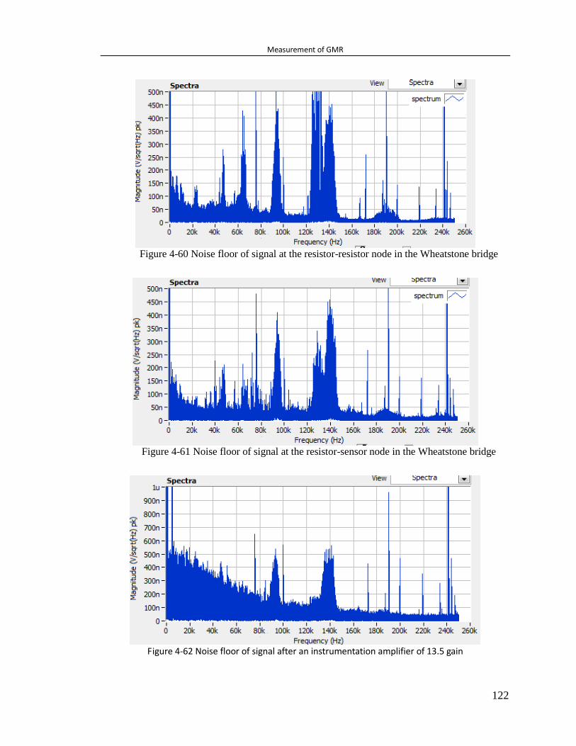
Measurement of GMR
122
Figure 4-60 Noise floor of signal at the resistor-resistor node in the Wheatstone bridge
Figure 4-61 Noise floor of signal at the resistor-sensor node in the Wheatstone bridge
Figure 4-62 Noise floor of signal after an instrumentation amplifier of 13.5 gain

Measurement of GMR
123
Figure 4-63 Noise floor of signal after an instrumentation amplifier after a low pass filter
Figure 4-64 Noise floor of 85 mV DC signal provided by a 7.5 V battery and 10 kΩ
potentiometer
1.94 1.96 1.98 2 2.02 2.04 2.06 2.08
x 104
0
0.5
1
1.5
2
2.5
3
3.5
x 10-5 best: canceling and hamming window
Hz
sig
nal am
plit
ude
1.92 1.94 1.96 1.98 2 2.02 2.04 2.06 2.08
x 104
0
0.5
1
1.5
2
2.5
x 10-5 best: canceling and hamming window
Hz
sig
nal am
plit
ude
Figure 4-65 Left shows the spectrum of a 20 kHz sine signal generated by a function
generator. Right shows the spectrum of a 20 kHz sine signal generated by DAQ itself.

Measurement of GMR
124
4.11 Other development
4.11.1 Microcontroller Developments
Microcontroller dsPIC33FJ128MC802 has the capability of performing ADC at 1M
Sample/second, with resolution 10 bit. A Sin wave and square wave are generated by
function generator and digitized by the microcontroller as shown in Figure 4-66 and Figure
4-67. The DSP core can do FFT of input time signal as shown in Figure 4-68, and find the
peak frequency and peak amplitude. It also can communicate with computer through
USB at the baud rate of 115200 to receive the command from computer and send out the
data to computer.
Figure 4-66 A 100 kHz Sin signal sampled by a microcontroller.

Measurement of GMR
125
0 1 2 3
x 10-4
0
0.2
0.4
0.6
0.8
1
1.2
1.4
1.6
1.8
am
plit
ude (
V)
time (s)
Microcontroller ADC sampling of 100KHz square signal
Figure 4-67 A 100 kHz square wave sampled by a microcontroller.
0 0.5 1 1.5 2 2.5 3 3.5 4 4.5 5
x 105
1.64
1.66
1.68
1.7
1.72
1.74
1.76
am
plit
ude (
V)
frequency (Hz)
Microcontroller FFT of 100KHz square signal
Figure 4-68 Voltage spectrum of Figure 4-67 calculated by FFT module in DSP core in
μC. The peak frequency is 0x00018CB4 = 101556 Hz shows the clock mismatch between
function generator and μC.

Measurement of GMR
126
4.11.2 Demodulation circuits
Since DAQ is not perfect in term of noise, an analog circuit can help to increase the
SNR. The idea is to use the exact input signal to the GMR to demodulate the output
signal to low frequency region. The working principle is similar to that of lock-in
amplifier. In the Figure 4-69, A 2 kHz current and 200 Hz field generated by function
generator are applied to the sensor. 1.8 kHz and 2.2 kHz mixing frequencies are
generated. A multiplier AD743 is used to demodulate the high frequency signal to low
frequency region by modulating 2 kHz input signal. The demodulated signal has the
spectrum shown in Figure 4-70. Also the DC offset can be trimmed, thus the signal can be
amplified effectively.
Figure 4-69 A 2 kHz and a 200 Hz signal are applied to the sensor. The output shows the
mixing frequencies 1.8 kHz and 2.2 kHz.

Measurement of GMR
127
Figure 4-70 By modulating 2 kHz input with the output signal in Figure 4-69, the mixing
terms are demodulated in 200 Hz.
4.11.3 Function Generating Circuit
To develop a hand-held system, a XR2206 can be used to generate the sine wave
with frequency from 0.01 Hz to 1 MHz. A 3.5 kHz sine wave generated by XR2206 is
shown below.
Figure 4-71 a 3.5 kHz sine wave generated by XR2206

Measurement of GMR
128
37 Karl F. Anderson, ‘Current Loop Signal Conditioning: Practical Applications’, NASA
Technical Memorandum 4636, Jan. 1995. 38Biosensors and Bioelectronics 22 (2007) 2366–2370 39 Figure 6.37, Chapter 6, Fundamentals of the Metal-Oxide-Semiconductor Field-Effect
Transistor’, Donald A. Neamen, ‘an introduction to Semiconductor devices.’ 40 Data Sheet of ‘NI USB-6289’, National Instruments 41 Data sheet of ‘OPA827’, TI, Nov. 2006 42 Data sheet of ‘ADG 1606’, Analog Devices 43 Data sheet of ‘INA163’, TI, 16 May 2005

Conclusion and Outlook
129
Chapter 5 Conclusion and Outlook
5.1 Conclusion
Superparamagnetic Nanoparticles (MNPs) have been successfully detected by
using a search coil based scheme for volume detection and by using a Giant
Magneto-Resistance (GMR) sensor for surface detection.
In search coil detection scheme, magnetic and hydrodynamic dynamic response of
MNP to the external magnetic field has been analyzed. Proper model for MNP relaxation
has been proposed, and the results of MNPs in different coating and solution have been
compared with the experiments. The approach to colorize different MNPs by mixing
frequency method is also simulated and experimentally verified. Besides MNPs,
magnetic thin film and bulk material has also been studied using mixing frequency
method.
In GMR detection scheme, various proteins have been detected using MNPs as
probes in the sandwich structure. The detection sensitivity is higher than the current
ELISA method, and the range covers 5 to 6 orders. Multiple capture antibodies can be
printed on the same chip to analyze the one patient sample. Although the exact detection
model of GMR is not very accurate, the experiments still show very reliable and
repeatable results. GMR noise, protection defects, and bad connections may also affect
the sensitivity to a certain level. These issues will be addressed in the future improvement
in the fabrication process.
5.2 Outlook
In search coil detection scheme, the current frequency range only covers the audio
frequency. By increasing the frequency and increasing the field amplitude, the sensitivity
of the detection will increase proportionally. By improving the sampling rate and

Conclusion and Outlook
130
resolution in the digital circuit, the SNR will also increase. More advanced analog circuit
can be used to reduce the burden of DAQ and reduce the noise from DAQ. The coil
design can be further improved to fit the applications of small scale detection or high
frequency detection. Coil, in the form of transmission line, can study the FMR of
magnetic material. One rough approach to study the RF response of MNPs is presented in
the section FMR in the appendix.
In GMR detection scheme, GMR detection model needs to be fully understood in
order to design an optimal sensor. The protection layer needs to be more reliable so that
the nonmagnetic factors will not cause the drift of the sensor signal. The issue of current
leakage to the semiconductor needs to be addressed, because the unnecessary
conductance and susceptance of the semiconductor will decrease the signal and introduce
noise. Also the noise spectrum of the GMR needs further study to design a better circuit
for optimal SNR. Furthermore, the GMR technology can be incorporated with other
detection method, such as ultrasound, magnetic semiconductor, and etc.
Magnetic bio-sensors, compared to currently popular optical bio-sensors, have
shown very promising market. The natural background noise is much less than optical
method, which can push the detection limit further down. Also the magnetic sensors are
more easily compatible with CMOS technology, which makes them good candidates for
point-of-care devices. As the technology has been used for hard disk drive for several
decades, magnetic bio-sensor benefits from very mature industry and researches. Plus
with the properties of cheap cost and light weight, magnetic bio-sensor will have a bright
future.

Conclusion and Outlook
131
Bibliography
1Robert C. O’Handley, Modern Magnetic Materials: Principles and Applications. Publication Date: Nov. 26, 1999| ISBN-10: 0471155667| ISBN-13:978-0471155669| Edition: 1
2 Superparamagnetism, (Oct. 22nd, 2012), from
http://en.wikipedia.org/wiki/Superparamagnetism 3 Superparamagnetism, (Oct. 22nd, 2012), from
http://lmis1.epfl.ch/webdav/site/lmis1/shared/Files/Lectures/Nanotechnology%20for%20engineers/Archives/2004_05/Superparamagnetism.pdf 4 Y. Jing, S. He, T. Kline, Y. Xu and J.P. Wang, ‘High-Magnetic-Moment Nanoparticles for Biomedicine’, 31st Annual International Conference of the IEEE EMBS, Minneapolis, Minnesota, USA, September 2-6, 2009. 5 K. M. Krishnan, A. B. Pakhomov, Y. Bao, et al.,‘Nanomagnetism and spin electronics: materials, microstructure and novel properties.’ J Mater Sci 41 (2006) 793-815. 6 Landau-Lifshitz-Gilbert equation, (Oct. 23rd, 2012), from
http://en.wikipedia.org/wiki/Landau%E2%80%93Lifshitz%E2%80%93Gilbert_equation 7 W. T. Coffey, P. J. Gregg, and Y. P. Kalmykov, ‘On the Theory of Debye and Néel Relaxation of Single Domain Ferromagnetic Particles’, in Advances in Chemical Physics, edited by I. Prigogine and S. A. Rice (Wiley, New York, 1993), Vol. 83, p. 263 8 B K P Scaife, ‘On the low-field, low-frequency susceptibility of magnetic fluids’, J. Phys. D:
Appl. Phys. 19 (1986) L195-L197
9 Vibrating sample magnetometer, (Oct. 31st, 2012), from
http://en.wikipedia.org/wiki/Vibrating_Sample_Magnetometer
10 Scanning electron microscope, (Oct. 31st, 2012), from
http://en.wikipedia.org/wiki/Scanning_electron_microscope
11 Transmission electron microscope, (Oct. 31st, 2012), from
http://en.wikipedia.org/wiki/Transmission_electron_microscopy 12 Dynamic light scattering, (Oct. 31st, 2012), from
http://en.wikipedia.org/wiki/Dynamic_light_scattering 13 J. Lenz, IEEE Proceedings, 78, 973, (1990)
14 Caruso, Michael J; Tamara Bratland; Carl H Smith, PhD; and Robert Schneider, “A New
Perspective on Magnetic Field Sensing,” Honeywell Inc, May 1998, www.ssec.honeywell.com/
magnetic/datasheets/new_pers.pdf
15 http://www.boulder.nist.govdiv81881803MagneticDevicesandNanoStructuresindex.html
16 Quantum Design, San Diego, CA, ‘http://www.qdusa.com/products/ppms.html’

Conclusion and Outlook
132
17 Imego Institute, Göteborg, SWEDEN, ‘http://www.imego.com/Products/dynomag/index.aspx’ 18 P.C. Fannin, B.K.P. Scaife, J. Magn.Magn.Mater.72, 95 (1988)
19 Magnetic dipole, 11/9/2012, from ‘http://en.wikipedia.org/wiki/Magnetic_dipole’
20 http://www.oceannanotech.com/upload/090604131348592520yef2g1.pdf
21 T.L. Paoli and J.F. Svacek, Rev. Sci. instrum., 47, 9 (1976)
22
Petr I. Nikitin, Petr M. Vetoshko, and Tatiana I. Ksenevich, J. Magn. Magn.Mater.311, 445 (2007)
23
Hans-Joachim Krause, Norbert Wolters, Yi Zhang, Andreas Offenhausser, Peter Miethe, Martin H.F.
Meyer, Markus Hartmann, and Michael Keusgen, J. Magn. Magn.Mater.311, 436 (2007) 24 R.E. Rosensweig, J. Magn. Magn.Mater.252, 370 (2002)
25
M.I. Shliomis, Yu.L. Raikher, IEEE Trans. Magn. MAG-16, 237 (1980)
26J Dieckhoff, M. Schilling, and F. Ludwig, “Fluxgate based detection of magnetic nanoparticle dynamics
in a rotating magnetic field.”Appl. Phys. Lett., vol. 99, p. 112501, 2011
27 T. Yoshida, K. Enpuku, J. Dieckhoff, M. Schilling, and F. Ludwig, “Magnetic fluid dynamics in a
rotating magnetic field” J. Appl. Phys., vol. 111, pp. 053901, 2012
28 T. L. Paoli and J. F. Svacek, “Derivative measurement by frequency mixing,” Rev. Sci. Instrum., vol. 47,
p. 1016, 1976
29 W. T. Coffey, P. J. Cregg, and Y. P. Kalmykov, “On the theory of Debye and Néel relaxation of single
domain ferromagnetic particles,” Advances in Chemical Physics, vol. 83, p. 263, 1993
30 http://crca.ucsd.edu/~msp/techniques/v0.11/book-html/node86.html
31 Liang Tu, et. al. ‘Measurement of Brownian and Néel Relaxation of Magnetic Nanoparticles
by a Mixing-Frequency Method’, IEEE Transactions on Magnetics, Vol 49, No. 1, January
2013
32 K. Enpuku, T. Tanaka, Y. Tamai, F. Dang, N. Enomoto, J. Hojo, H. Kanzaki, and N. Usuki,
Jpn. J. Appl. Phys. 47, 7859 (2008)
33 C.M. Oireachtaigh, P.C. Fannin, J. Magn.Magn.Mater.320, 871 (2008)
34 B.K.P. Scaife, J. Phys. D: Appl. Phys. 19, 195 (1986)
35 C. Hong, C.C. Wu, Y.C. Chiu, S.Y. Yang, H.E. Horng, and H.C. Yang,Appl. Phys.Lett. 88,212512 (2006)
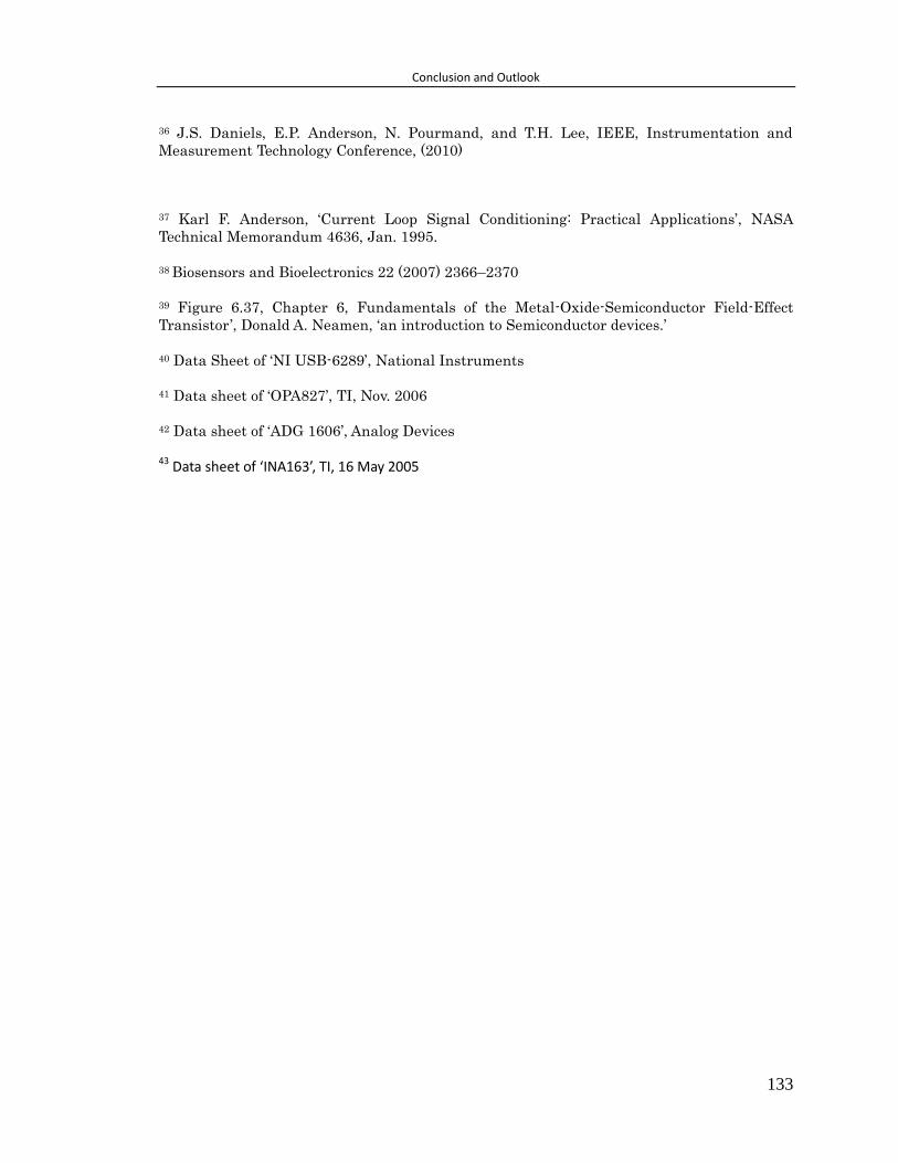
Conclusion and Outlook
133
36 J.S. Daniels, E.P. Anderson, N. Pourmand, and T.H. Lee, IEEE, Instrumentation and
Measurement Technology Conference, (2010)
37 Karl F. Anderson, ‘Current Loop Signal Conditioning: Practical Applications’, NASA
Technical Memorandum 4636, Jan. 1995.
38 Biosensors and Bioelectronics 22 (2007) 2366–2370
39 Figure 6.37, Chapter 6, Fundamentals of the Metal-Oxide-Semiconductor Field-Effect
Transistor’, Donald A. Neamen, ‘an introduction to Semiconductor devices.’
40 Data Sheet of ‘NI USB-6289’, National Instruments
41 Data sheet of ‘OPA827’, TI, Nov. 2006
42 Data sheet of ‘ADG 1606’, Analog Devices
43 Data sheet of ‘INA163’, TI, 16 May 2005

Conclusion and Outlook
134
Appendix
1. 1 FMR
Ferromagnetic resonance (FMR) is a spectroscopic technique to probe the
magnetization of ferromagnetic materials. 44
The resonance comes from the unpaired
electrons. The resonance frequency depends on the gyromagnetic ratio γ, and effective
magnetic field including external field and anisotropy field. For sphere sample, there is
no direction preference, and the resonance frequency is ω0 = γB0.45
As an illustration
shown in Figure 5-1, the resonance frequency has a linear dependence on the applied
field H. However, when pH=6, the MNPs have chemical binding affinity, and the stray
field of MNPs will affect each other. The resonance frequency is spread due to the
various interactions of MNPs, and the line width ∆H will be bigger.
46
pH= 6 pH= 8
pH=6
pH=8
pH changes line width
pH changes resonance frequency
Figure 5-1 Resonance frequency (left figure) and line width (right figure) of MNP
are dependence on pH of solution (dot represents pH=8; circle represents pH=6).46

Conclusion and Outlook
135
In order to detect the FMR of MNPs, a transmission line (Tline) is needed to deliver and
transmit the microwave. The microwave absorption of the MNPs will be detected through the
transmission and reflection coefficients measured by a network analyzer. The transmission line is
designed and fabricated based on a 4-layer PCB as shown in Figure 5-2. A simple in-planar spiral
is simulated in Sonnet and HFSS. The HFSS full-wave simulation tool can generate the EM wave
distribution along the line Figure 5-4. The Sonnet simulator can calculate the S-parameters Figure
5-5 and input impedance Figure 5-7 along frequency. There is no simple way to simulate the
effects from the MNPs, so I simply increase the permeability μr=2 to see how the results will be
affected. Figure 5-6 and Figure 5-7Figure 5-8 show that the peaks of S-parameters and input
impedance will be shifted and changed. Increasing the turns of the coil shown in Figure 5-9, more
complicated pattern of S-parameters is generated in Figure 5-10. By carefully design the shape of
the transmission line, we will find an optimal detection method for the MNPs. However, here as a
first try, co-planar Tline with and without gap, planar coil with different turns and sizes are
designed in Figure 5-11. All the connection lines are designed in 50Ω configuration to decrease
the signal loss to/from the sensor spot. The MNPs samples are iron oxide particles, and a
permanent magnet is used to generate non-uniform field. From left to right, the measurement of
Tline1 to Tline6 are plotted from Figure 5-12 to Figure 5-17. The blue lines show the difference of
S-parameters by adding MNPs. The green lines show the differences of S-parameters by adding
MNPs with a permanent magnet. There is clear evidence that the MNPs affect the microwave
transmission on the Tline. However, the FMR effects need further studies.
Figure 5-2 Structure of a 4-layer PCB47

Conclusion and Outlook
136
Figure 5-3 Coil Design in Sonnet simulation
Figure 5-4 Magnetic field distribution by HFSS

Conclusion and Outlook
137
Figure 5-5 S-parameter measurement in Sonnet simulation
Figure 5-6 S-parameter measurement in Sonnet simulation.μr is changed to 2 to
represent MNPs.

Conclusion and Outlook
138
Figure 5-7 Input impedance measurement in Sonnet simulation.
Figure 5-8 Input impedance measurement in Sonnet simulation. μr is changed to 2 to
represent MNPs.

Conclusion and Outlook
139
Figure 5-9 Coil Design with more turns in Sonnet simulation
Figure 5-10 S-parameter measurement in Sonnet simulation

Conclusion and Outlook
140
Figure 5-11 PCB design of various transmission lines
0 5 10 15 20 25 30 35 400
0.1
0.2TLine1 S11
0 5 10 15 20 25 30 35 400
0.2
0.4
GHz
TLine1 S21
MNP
MNP + Magnet
MNP
MNP + Magnet
Figure 5-12 S-parameter of TLine1

Conclusion and Outlook
141
0 5 10 15 20 25 30 35 400
0.5
1TLine2 S11
0 5 10 15 20 25 30 35 400
0.01
0.02
0.03
GHz
TLine2 S21
MNP
MNP + Magnet
MNP
MNP + Magnet
Figure 5-13 S-parameter of TLine2
0 5 10 15 20 25 30 35 400
0.2
0.4TLine3 S11
0 5 10 15 20 25 30 35 400
0.02
0.04
0.06
GHz
TLine3 S21
MNP
MNP + Magnet
MNP
MNP + Magnet
Figure 5-14 S-parameter of TLine3

Conclusion and Outlook
142
0 5 10 15 20 25 30 35 400
0.02
0.04TLine4 S11
0 5 10 15 20 25 30 35 400
0.01
0.02
GHz
TLine4 S21
MNP
MNP + Magnet
MNP
MNP + Magnet
Figure 5-15 S-parameter of TLine4
0 5 10 15 20 25 30 35 400
0.5
1TLine5 S11
0 5 10 15 20 25 30 35 400
0.05
0.1
GHz
TLine5 S21
MNP
MNP + Magnet
MNP
MNP + Magnet
Figure 5-16 S-parameter of TLine5

Conclusion and Outlook
143
0 5 10 15 20 25 30 35 400
1
2TLine6 S11
0 5 10 15 20 25 30 35 400
0.2
0.4
GHz
TLine6 S21
MNP
MNP + Magnet
MNP
MNP + Magnet
Figure 5-17 S-parameter of TLine6

Conclusion and Outlook
144
44 http://en.wikipedia.org/wiki/Ferromagnetic_resonance
45 Charles Kittel, ‘Introduction to Solid State Physics’. 8th edition.
46‘Relaxation of Polymer Coated …’, University of Alabama, IEEE,Vol 46, No. 6, June 2010
47http://www.4pcb.com/index.php?load=content&page_id=242