Traffic-Driven Power Saving in Operational 3G CellularNetworks

Chunyi Peng, Suk-Bok Lee, Songwu Lu, Haiyun Luo∗, Hewu Li+UCLA Computer Science, Los Angeles, CA 90095, USA; Tsinghua University, Beijing 100084, China+

{chunyip,sblee, slu}@cs.ucla.edu, hluo@live.com∗, lihewu@cernet.edu.cn+

ABSTRACTBase stations (BSes) in the 3G cellular network are not energyproportional with respect to their carried traffic load. Ourmea-surements show that 3G traffic exhibits high fluctuations both intime and over space, thus incurring energy waste. In this paper,we propose a profile-based approach to green cellular infrastruc-ture. We profile BS traffic and approximate network-wide energyproportionality using non-load-adaptive BSes. The instrument isto leverage temporal-spatial traffic diversity and node deploymentheterogeneity, and power off under-utilized BSes under light traf-fic. Our evaluation on four regional 3G networks shows that thissimple scheme yields up to53% energy savings in a dense largecity and23% in a sparse, mid-sized city.

Categories and Subject DescriptorsC.2.1 [Computer Systems Organization]: Computer-Communication Networks—Network Architecture and Design;C.4 [Computer Systems Organization]: Performance of Systems

General TermsDesign, Measurement, Performance

KeywordsEnergy Efficiency, Cellular Networks, 3G Network Traffic

1. INTRODUCTIONWe are currently experiencing surging energy consumptionson

the wireless cellular infrastructure. Recent reports showenergyconsumption of mobile networks would reach 124.4B KWh in2011 [3], and the power bill is expected to double in five yearsfor one Chinese mobile operator [19]. To build a green cellularnetwork, we need to first improve the most critical subsystemthatis the dominant contributing factor to overall energy. In the 3Gcontext, it is the base station (BS) subsystem. BSes consumeabout

∗This work was done when he collaborated with UCLA as an in-dependent contributor not associated with his current affiliation.

Permission to make digital or hard copies of all or part of this work forpersonal or classroom use is granted without fee provided that copies arenot made or distributed for profit or commercial advantage and that copiesbear this notice and the full citation on the first page. To copy otherwise, torepublish, to post on servers or to redistribute to lists, requires prior specificpermission and/or a fee.MobiCom’11,September 19–23, 2011, Las Vegas, Nevada, USA.Copyright 2011 ACM 978-1-4503-0492-4/11/09 ...$10.00.

80% of overall infrastructure energy, while the user clients typicallytake around 1% [15].

In this paper, we seek to make the 3G infrastructure more energyefficient. We use real traffic traces, actual BS deployment map andmeasured BS power consumption, collected from four regional 3Gnetworks, each of which has 45 to 177 BSes and is operated bya largest mobile operator in the world. Our analysis revealsthat,3G traffic load exhibits wide-range fluctuations both in timeandover space. However, energy consumption of current networks isnot load adaptive. The used energy is unproportionally large underlight traffic. The root cause is that each BS is not energy propor-tional, with more than 50% spent on cooling, idle-mode signalingand processing, which are not related to the runtime traffic load.

We design a solution that approximates an energy-proportional(EP) 3G system using non-EP BS components, in order to copewith temporal-spatial traffic dynamics. The main instrument of ourproposal is to completely power off under-utilized BSes when theirtraffic load is light and power them on when the traffic load be-comes heavy. The challenge is to devise a distributed solution thatuses a small set of active BSes, while satisfying three requirementsof traffic capacity, communication coverage, and minimal on/offswitching of each BS. To this end, we take a location-dependentprofile-based approach. We divide the network into grids, sothatBSes in each local cell can replace each other when serving userclients. We then perform location-dependent profiling to estimatethe aggregate traffic among BSes in the grid. Based on the peak/idleof the traffic profile, we decide the corresponding set of active BSesfor each duration. It turns out that, if we select the active sets ap-propriately, we only need to power on a sleep BS and shut down anactive BS at most only once during each 24-hour period.

Our evaluation using real traces shows that our scheme leadstoaverage daily energy saving of 52.7%, 46.6%, 30.8% and 23.4%in the four regional 3G networks. The savings are more signifi-cant during midnight and weekends and in dense deployment ar-eas, while the miss rate to deny client requests is kept lowerthan0.1% in the worst case. While our scheme saves energy on cellularinfrastructure, it does negatively increase client power for uplinktransmission duringidle hours (e.g., late nights and weekends).

The rest of the paper is organized as follows. Section 2 intro-duces 3G background and Section 3 explores the operating energy-load curve in 3G networks and models BS power consumption.Section 4 analyzes 3G traffic, and Section 5 describes the proposedsolution as well as its implementation within the 3G standard. Sec-tion 6 evaluates the performance and Section 7 discusses therelatedwork. Section 8 concludes the paper.

2. BACKGROUNDThe 3G network infrastructure has two main parts of radio access

Power

SupplyUtility

AC/

Cooling

BBU

BBU48V

Environment

Monitoring

BBU

RRU

RRU

RRU

Feeder

R

N

C

Transmission

Devices

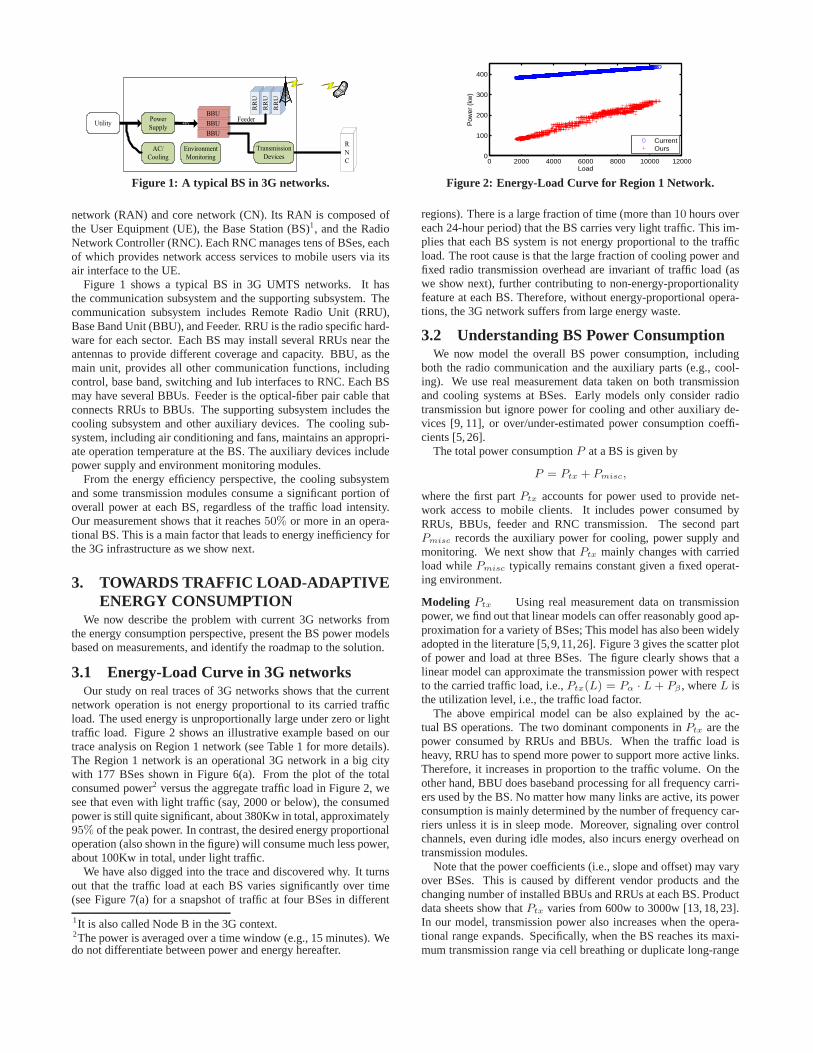
Figure 1: A typical BS in 3G networks.

network (RAN) and core network (CN). Its RAN is composed ofthe User Equipment (UE), the Base Station (BS)1, and the RadioNetwork Controller (RNC). Each RNC manages tens of BSes, eachof which provides network access services to mobile users via itsair interface to the UE.

Figure 1 shows a typical BS in 3G UMTS networks. It hasthe communication subsystem and the supporting subsystem.Thecommunication subsystem includes Remote Radio Unit (RRU),Base Band Unit (BBU), and Feeder. RRU is the radio specific hard-ware for each sector. Each BS may install several RRUs near theantennas to provide different coverage and capacity. BBU, as themain unit, provides all other communication functions, includingcontrol, base band, switching and Iub interfaces to RNC. Each BSmay have several BBUs. Feeder is the optical-fiber pair cablethatconnects RRUs to BBUs. The supporting subsystem includes thecooling subsystem and other auxiliary devices. The coolingsub-system, including air conditioning and fans, maintains an appropri-ate operation temperature at the BS. The auxiliary devices includepower supply and environment monitoring modules.

From the energy efficiency perspective, the cooling subsystemand some transmission modules consume a significant portionofoverall power at each BS, regardless of the traffic load intensity.Our measurement shows that it reaches50% or more in an opera-tional BS. This is a main factor that leads to energy inefficiency forthe 3G infrastructure as we show next.

3. TOWARDS TRAFFIC LOAD-ADAPTIVEENERGY CONSUMPTION

We now describe the problem with current 3G networks fromthe energy consumption perspective, present the BS power modelsbased on measurements, and identify the roadmap to the solution.

3.1 Energy-Load Curve in 3G networksOur study on real traces of 3G networks shows that the current

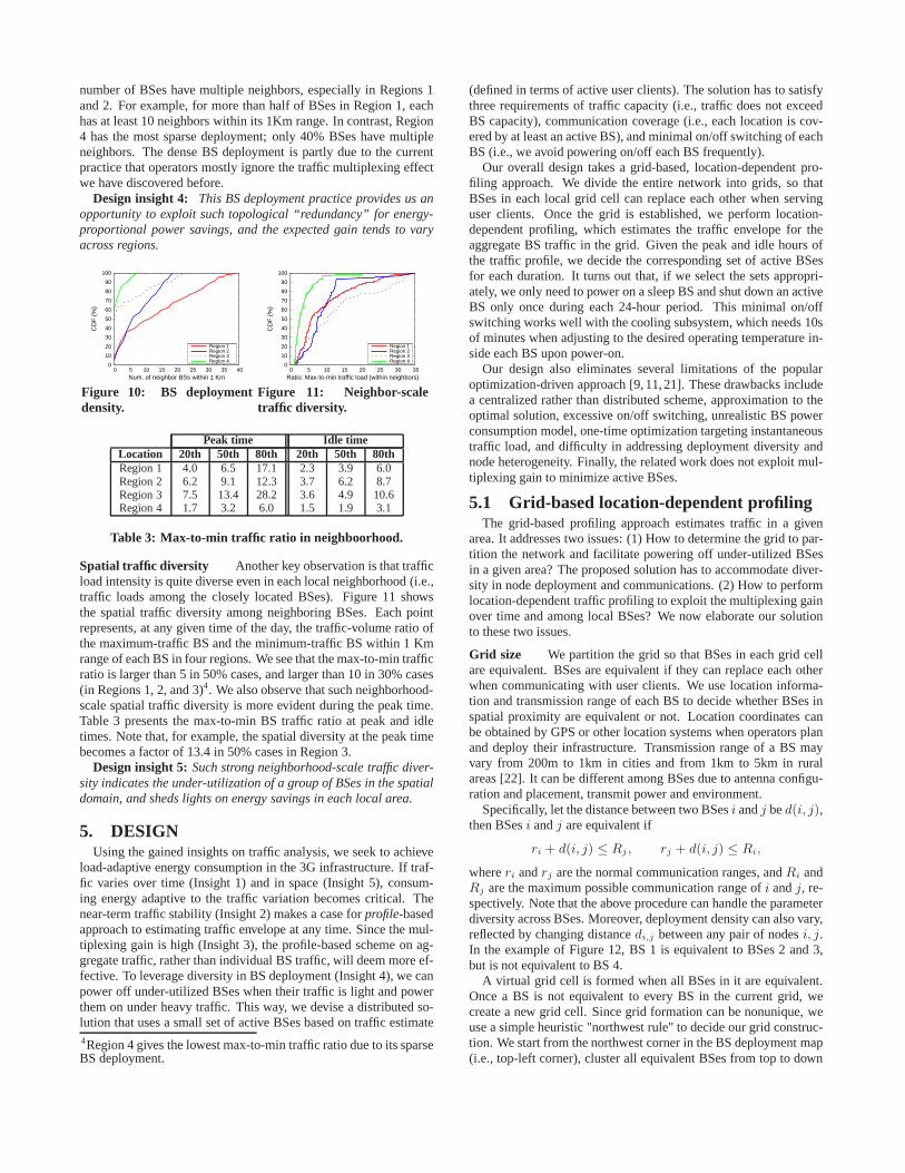
network operation is not energy proportional to its carriedtrafficload. The used energy is unproportionally large under zero or lighttraffic load. Figure 2 shows an illustrative example based onourtrace analysis on Region 1 network (see Table 1 for more details).The Region 1 network is an operational 3G network in a big citywith 177 BSes shown in Figure 6(a). From the plot of the totalconsumed power2 versus the aggregate traffic load in Figure 2, wesee that even with light traffic (say, 2000 or below), the consumedpower is still quite significant, about 380Kw in total, approximately95% of the peak power. In contrast, the desired energy proportionaloperation (also shown in the figure) will consume much less power,about 100Kw in total, under light traffic.

We have also digged into the trace and discovered why. It turnsout that the traffic load at each BS varies significantly over time(see Figure 7(a) for a snapshot of traffic at four BSes in different

1It is also called Node B in the 3G context.2The power is averaged over a time window (e.g., 15 minutes). Wedo not differentiate between power and energy hereafter.

0 2000 4000 6000 8000 10000 120000

100

200

300

400

Load

Pow

er (k

w)

CurrentOurs

Figure 2: Energy-Load Curve for Region 1 Network.

regions). There is a large fraction of time (more than10 hours overeach 24-hour period) that the BS carries very light traffic. This im-plies that each BS system is not energy proportional to the trafficload. The root cause is that the large fraction of cooling power andfixed radio transmission overhead are invariant of traffic load (aswe show next), further contributing to non-energy-proportionalityfeature at each BS. Therefore, without energy-proportional opera-tions, the 3G network suffers from large energy waste.

3.2 Understanding BS Power ConsumptionWe now model the overall BS power consumption, including

both the radio communication and the auxiliary parts (e.g.,cool-ing). We use real measurement data taken on both transmissionand cooling systems at BSes. Early models only consider radiotransmission but ignore power for cooling and other auxiliary de-vices [9, 11], or over/under-estimated power consumption coeffi-cients [5,26].

The total power consumptionP at a BS is given by

P = Ptx + Pmisc,

where the first partPtx accounts for power used to provide net-work access to mobile clients. It includes power consumed byRRUs, BBUs, feeder and RNC transmission. The second partPmisc records the auxiliary power for cooling, power supply andmonitoring. We next show thatPtx mainly changes with carriedload whilePmisc typically remains constant given a fixed operat-ing environment.

Modeling Ptx Using real measurement data on transmissionpower, we find out that linear models can offer reasonably good ap-proximation for a variety of BSes; This model has also been widelyadopted in the literature [5,9,11,26]. Figure 3 gives the scatter plotof power and load at three BSes. The figure clearly shows that alinear model can approximate the transmission power with respectto the carried traffic load, i.e.,Ptx(L) = Pα · L+ Pβ , whereL isthe utilization level, i.e., the traffic load factor.

The above empirical model can be also explained by the ac-tual BS operations. The two dominant components inPtx are thepower consumed by RRUs and BBUs. When the traffic load isheavy, RRU has to spend more power to support more active links.Therefore, it increases in proportion to the traffic volume.On theother hand, BBU does baseband processing for all frequency carri-ers used by the BS. No matter how many links are active, its powerconsumption is mainly determined by the number of frequencycar-riers unless it is in sleep mode. Moreover, signaling over controlchannels, even during idle modes, also incurs energy overhead ontransmission modules.

Note that the power coefficients (i.e., slope and offset) mayvaryover BSes. This is caused by different vendor products and thechanging number of installed BBUs and RRUs at each BS. Productdata sheets show thatPtx varies from 600w to 3000w [13, 18, 23].In our model, transmission power also increases when the opera-tional range expands. Specifically, when the BS reaches its maxi-mum transmission range via cell breathing or duplicate long-range

0 50 1000

500

1000

1500

2000

2500

Load

Pow

er (

w)

p = 8.25x + 1225

p = 8.25x+815

p = 5.38x + 600

Figure 3: Ptxvs. load at 3 BSes.

−20 0 20 400

500

1000

1500

2000

2500

Temperature (oC)

Pow

er (

w)

Figure 4: Pmisc vs. temperature.D1/Winter D2/Spring D3/Summer D4/Fall

0

500

1000

1500

2000

2500

Powe

r (w)

4 daysone year (1−25−50−75−99th)

Figure 5: Pmisc on 4-day and 1-year time scales.

radios (see Section 5.3 for details), we model that the poweralsogrows in proportion to the traffic load but uses a larger coefficientPa, say,Pa doubles at its maximum range. Our design and evalua-tion consider such diversity factors.

Modeling Pmisc We focus on modeling the cooling (i.e., airconditioner) power consumption since it is the dominant factor inPmisc based on real measurement. It depends on the amount of theextracted heat and the desired operating temperature. It also varieswith chillers that use a variety of compressors and drivers.Previouswork does not model this part, though it is known that coolingmayconsume about 50% power at BSes [15].

Figure 4 shows the scatter plot of the cooling power and temper-ature at a BS in 2010. It can be seen that the cooling power mainlydepends on the temperature. It increases approximately linearlyfrom 1000w to 2000w when the environment temperature variesfrom−10oC to30oC (i.e., from winter to summer). We also checkdaily and yearly pattern in Figure 5. The upper line is the yearlypattern (1-25-50-75-99th percentile in 96 bins) that varies with fourseasons. The lower line is a 4-day measurement in early winter. Itshows that though the cooling power fluctuates slightly at differenthours of a day (e.g., BBUs and RRUs tend to raise the air temper-ature and the chiller workload). It can still be approximated as aconstant within a short period of time (say, a day), here in [1200w,1400w]. Over a larger time window (say, a year), it varies withthe external environment temperature. For simplicity, we assumepmisc remains constant on a daily basis but changes with seasons.

In summary, our analysis shows that each BS is not energy pro-portional to its carried load, mainly due to the residual factors ofPmisc andPβ . Recent efforts [12, 14] have been made to reducethem to some extent, but cannot eliminate them.

3.3 Roadmap to the SolutionGiven that 3G network is not energy proportional to traffic load,

our ultimate goal is to build a load-adaptive solution to energy sav-ings in operational 3G networks. To this end, we need to addressthree issues: (1) What are the characteristics of traffic load in oper-ational 3G networks? We use real traffic traces and BS deploymentmap to conduct detailed analysis on traffic dynamics both in timeand over space (Section 4); (2) Given the traffic dynamics, how canwe achieve network-wide energy proportionality (EP) usingnon-EP components shown in Section 3.2? We need a solution that canachieve load-adaptive energy operation using the current non-EPBS (Sections 5.1 and 5.2). (3) How can the proposed solution workwith the current 3G standard? The solution needs to be standardcompliant (Section 5.3). We next elaborate on these aspects.

4. 3G DATA TRAFFIC: DIVERSITY INTIME AND SPACE

In this section, we present our measurement results on 3G traf-fic diversity in both time and space, and show the design in-sights on how to improve the current 3G network’s non-energy-

proportionality. We use traces collected from the operational 3Gnetwork in four regions to study their temporal-spatial traffic pat-terns. All four regional networks are managed by one of the largestoperators in the world. Figure 6 shows the BS locations in thesefour regions; we hide the detailed deployment map for privacy con-cerns. They have different geographic scales and representdiversecity types: Region 1 is a large, populous city, Region 2 is a medium-size city, and Regions 3 and 4 are large cities in a large metropolitanarea. All regions have diverse residential and downtown areas. Thecoverage area and the number of BSes in each region are given inTable 1. Our data sets contain 15min-bin traffic volume records fortwo months from August 2010 to October 2010. For proprietaryreasons, the presented traffic volume is normalized by an arbitraryconstant, but normalization does not change the dynamic range inthe figures.

Region 1 Region 2 Region 3 Region 4Area (km) 11x11 8x4 16x28 30x45# BS 177 45 154 164BS density dense dense/normal normal/sparse sparse

Table 1: Basic statistics of 4-region traces.

4.1 Temporal Diversity

Temporal traffic dynamics We first find that each BS exhibitshigh traffic dynamics over time. Figure 7(a) plots the trafficload atfour individual BSes in different regions. We observe strong diur-nal patterns on both daily and weekly basis, alternating betweenpeak and idle durations3. We separate the weekday and week-end data here, and only present the weekday case unless explicitlystated; the result for weekend is similar.

To quantify the degree of temporal traffic dynamics, we computethe ratio of peak-to-idle traffic load at each BS in four regions. Wedefine the peak (/idle) duration of each BS as the hourh, whenit has the maximum (/minimum) traffic load (typically between10AM-18PM for peak, or 1AM-5AM for idle), plus two adjacenthours, i.e.,h−1 andh+1. Figure 7(b) presents CCDF of peak-to-idle traffic-load ratios in four regions. We see that the peak-to-idletraffic ratio is larger than 4 in most (70-90%) BSes, and the smallerratio (say, 2–4 in Region 1) is only due to relative small traffic vol-ume at BSes. We also study the effect of time window size (here,3hr) and find that large peak-to-idle ratios still exist whenthe win-dow is smaller than 8 hours.

Design insight 1: This result shows that the traffic distributionof each BS is quite diverse over time everywhere. Such strongtem-poral diversity indicates the under-utilization of each BSin the timedomain, resulting in system-wide energy inefficiency at BSes.

Near-term traffic stability We also observe that the trafficvolume is stable over short term (e.g., the same time of consecu-tive days), while it may slowly evolve over a long term (e.g.,26%global increase in 2010 [10]). Although the traffic load fluctuates3We use the term “idle” duration for light traffic cases in our work.

A

B

(a) Region 1

A

B

(b) Region 2

A

B

(c) Region 3

A

B

(d) Region 4

Figure 6: Base station locations in four regions. Dotted rectangles A and B indicate residential and downtown areas.

0

20

40

60

80

100

08/30 08/31 09/01 09/02 09/03 09/04 09/05 09/06

BS

traf

fic lo

ad (

norm

)

Date

BS1BS2BS3BS4

(a) One-week traffic pattern

0

20

40

60

80

100

0 4 8 12 16 20

Per

cent

age

(> ra

tio)

Ratio of peak-to-idle traffic load

Region 1Region 2Region 3Region 4

(b) Peak-to-idle traffic ratio

Figure 7: Temporal traffic diversity.

Traffic load variation in consecutive daysLocation 10th 30th 50th 70th 90thRegion 1 2.1% 6.7% 12.1% 20.1% 38.7%Region 2 1.9% 6.4% 11.8% 20.6% 45.0%Region 3 2.1% 6.8% 12.3% 20.4% 42.0%Region 4 2.0% 6.3% 11.4% 18.8% 36.6%

Table 2: Near-term stability in four regions. The values indi-cate the traffic difference between consecutive days.

over time, the time-of-the-day traffic at each BS is quite stable overconsecutive days (see Figure 7(a)). For example, BS1 has similartraffic load at 5 pm in Days 1 and 2, Days 2 and 3, and so on.

We first assess the similarity of near-term traffic by computingtheir autocorrelation at each BS with the time-lag factor being 24hours. Our results show that, in all four regions, the autocorrelationvalues are higher than 0.963 for 70% BSes – confirming strongcorrelation between traffic load during two consecutive days. Tofurther measure the near-term stability, we also compute the near-term traffic variationV (i, t) at timet at BSi:

V (i, t) = |R(i, tcur)−R(i, tprev)|/R(i, tprev),

whereR(i, tcur) andR(i, tprev) denote the traffic load of BSi attime t on the current day and on the previous day. Table 2 showsthe near-term variation statistics using our two-month data in fourregions. We see that, at any time, the traffic load differencein twoconsecutive days is less than 20% for 70% BSes. We also note thathigh variation values are mostly caused by the low traffic volumeat the idle time and their absolute values of traffic difference are,in fact, quite small. We further examine the impact of different ag-gregation granularity (e.g., from 15-min bins to several hours). Thenear-term variation increases as the aggregation granularity grows,but remains highly stable when the window is smaller than 2 hours.

Design insight 2: The near-term stability result makes a casefor traffic profiling to estimate the next day’s traffic trend and moti-vates us to develop power-saving schemes using traffic profiles. Themeasurement also indicates that hourly traffic aggregationachievesgood balance between estimation accuracy and simplicity.

Time-domain multiplexing diversity We find that the aggre-

gate traffic load in a region hardly reaches the aggregate BS capac-ity in the region. To verify such a trend, we define time-domain“multiplexing” gainM(t) as the ratio of the sum of the peak trafficat each BS (i.e., lower bound of BS capacity) to the aggregatetrafficload at timet in the region:M(t) =

∑iR(i, tmax)/

∑iR(i, t),

whereR(i, t) is the traffic load of BSi at timet; tmax is the peaktraffic time. Figure 8 plots the multiplexing gainsM(t) in four re-gions. We see that the multiplexing gain is around 2 even duringdaytime in all regions. Note that the gain can be even larger inreality because the operators often deploy BSes with much largercapacity than the actual traffic demand to account for forthcom-ing market growth. The root cause for large multiplexing gain isthat not all BSes reach their peak load simultaneously. We studythe peak hour distribution in subregions A (residence area)and B(business area) and find that the peak hour spans from 10 AM to6 PM in A, and from 4 PM to 8 PM in B (see Figure 9). The op-erator has to deploy the infrastructure that can accommodate thepeak traffic at each location, even though the peak load may onlylast two or three hours a day. As the peak hour varies with eachlocation, the deployed capacity (i.e., the sum of each BS’s capac-ity) is much larger than the actual traffic volume at the time.Notethat, our observation also explains why current operators tend to beoverly conservative in BS deployment density, since they largelyignore the multiplexing effect of traffic load.

08:00 10:00 12:00 14:00 16:00 18:00 20:00 22:00

1

2

3

4

5

TM

Gai

n

Region 1Region 2Region 3Region 4

Figure 8: Time multiplexinggain.

10 12 14 16 18 20 22 10 12 14 16 18 20 220

0.05

0.1

0.15

0.2

0.25

0.3

Pro

babl

ity

a p pa

Subregion A (Residence) Subregion B (Business)

Figure 9: Peak hour distribu-tion.

Design insight 3: This multiplexing gain shows that the aggre-gate BS capacity is highly under-utilized in each region. Italso ex-plains why current BS deployment tends to be overly conservativein operational networks. The inherent temporal-spatial diversityopens venue for energy savings via aggregating traffic load.

4.2 Spatial Diversity

Diverse BS deployment density The BS deployment densityvaries across locations (see Figure 6 for location distributions). Inthe hot spots of a city (e.g., subregion B), more BSes are provi-sioned, thus creating location-dependent diversity. Figure 10 de-picts the distribution of the number of neighbors per BS (within 1Km, which is the typical communication range of many BS prod-ucts [22]), representing the BS deployment density in four regions.We see that the deployment density is quite diverse across differ-ent regions, as well as in the same region. We also see that a large

number of BSes have multiple neighbors, especially in Regions 1and 2. For example, for more than half of BSes in Region 1, eachhas at least 10 neighbors within its 1Km range. In contrast, Region4 has the most sparse deployment; only 40% BSes have multipleneighbors. The dense BS deployment is partly due to the currentpractice that operators mostly ignore the traffic multiplexing effectwe have discovered before.

Design insight 4: This BS deployment practice provides us anopportunity to exploit such topological “redundancy” for energy-proportional power savings, and the expected gain tends to varyacross regions.

0

10

20

30

40

50

60

70

80

90

100

0 5 10 15 20 25 30 35 40

CD

F (

%)

Num. of neighbor BSs within 1 Km

Region 1Region 2Region 3Region 4

Figure 10: BS deploymentdensity.

0

10

20

30

40

50

60

70

80

90

100

0 5 10 15 20 25 30 35

CD

F (

%)

Ratio: Max-to-min traffic load (within neighbors)

Region 1Region 2Region 3Region 4

Figure 11: Neighbor-scaletraffic diversity.

Peak time Idle timeLocation 20th 50th 80th 20th 50th 80thRegion 1 4.0 6.5 17.1 2.3 3.9 6.0Region 2 6.2 9.1 12.3 3.7 6.2 8.7Region 3 7.5 13.4 28.2 3.6 4.9 10.6Region 4 1.7 3.2 6.0 1.5 1.9 3.1

Table 3: Max-to-min traffic ratio in neighboorhood.

Spatial traffic diversity Another key observation is that trafficload intensity is quite diverse even in each local neighborhood (i.e.,traffic loads among the closely located BSes). Figure 11 showsthe spatial traffic diversity among neighboring BSes. Each pointrepresents, at any given time of the day, the traffic-volume ratio ofthe maximum-traffic BS and the minimum-traffic BS within 1 Kmrange of each BS in four regions. We see that the max-to-min trafficratio is larger than 5 in 50% cases, and larger than 10 in 30% cases(in Regions 1, 2, and 3)4. We also observe that such neighborhood-scale spatial traffic diversity is more evident during the peak time.Table 3 presents the max-to-min BS traffic ratio at peak and idletimes. Note that, for example, the spatial diversity at the peak timebecomes a factor of 13.4 in 50% cases in Region 3.

Design insight 5:Such strong neighborhood-scale traffic diver-sity indicates the under-utilization of a group of BSes in the spatialdomain, and sheds lights on energy savings in each local area.

5. DESIGNUsing the gained insights on traffic analysis, we seek to achieve

load-adaptive energy consumption in the 3G infrastructure. If traf-fic varies over time (Insight 1) and in space (Insight 5), consum-ing energy adaptive to the traffic variation becomes critical. Thenear-term traffic stability (Insight 2) makes a case forprofile-basedapproach to estimating traffic envelope at any time. Since the mul-tiplexing gain is high (Insight 3), the profile-based schemeon ag-gregate traffic, rather than individual BS traffic, will deemmore ef-fective. To leverage diversity in BS deployment (Insight 4), we canpower off under-utilized BSes when their traffic is light andpowerthem on under heavy traffic. This way, we devise a distributedso-lution that uses a small set of active BSes based on traffic estimate4Region 4 gives the lowest max-to-min traffic ratio due to its sparseBS deployment.

(defined in terms of active user clients). The solution has tosatisfythree requirements of traffic capacity (i.e., traffic does not exceedBS capacity), communication coverage (i.e., each locationis cov-ered by at least an active BS), and minimal on/off switching of eachBS (i.e., we avoid powering on/off each BS frequently).

Our overall design takes a grid-based, location-dependentpro-filing approach. We divide the entire network into grids, so thatBSes in each local grid cell can replace each other when servinguser clients. Once the grid is established, we perform location-dependent profiling, which estimates the traffic envelope for theaggregate BS traffic in the grid. Given the peak and idle hoursofthe traffic profile, we decide the corresponding set of activeBSesfor each duration. It turns out that, if we select the sets appropri-ately, we only need to power on a sleep BS and shut down an activeBS only once during each 24-hour period. This minimal on/offswitching works well with the cooling subsystem, which needs 10sof minutes when adjusting to the desired operating temperature in-side each BS upon power-on.

Our design also eliminates several limitations of the popularoptimization-driven approach [9,11,21]. These drawbacksincludea centralized rather than distributed scheme, approximation to theoptimal solution, excessive on/off switching, unrealistic BS powerconsumption model, one-time optimization targeting instantaneoustraffic load, and difficulty in addressing deployment diversity andnode heterogeneity. Finally, the related work does not exploit mul-tiplexing gain to minimize active BSes.

5.1 Grid-based location-dependent profilingThe grid-based profiling approach estimates traffic in a given

area. It addresses two issues: (1) How to determine the grid to par-tition the network and facilitate powering off under-utilized BSesin a given area? The proposed solution has to accommodate diver-sity in node deployment and communications. (2) How to performlocation-dependent traffic profiling to exploit the multiplexing gainover time and among local BSes? We now elaborate our solutionto these two issues.

Grid size We partition the grid so that BSes in each grid cellare equivalent. BSes are equivalent if they can replace eachotherwhen communicating with user clients. We use location informa-tion and transmission range of each BS to decide whether BSesinspatial proximity are equivalent or not. Location coordinates canbe obtained by GPS or other location systems when operators planand deploy their infrastructure. Transmission range of a BSmayvary from 200m to 1km in cities and from 1km to 5km in ruralareas [22]. It can be different among BSes due to antenna configu-ration and placement, transmit power and environment.

Specifically, let the distance between two BSesi andj bed(i, j),then BSesi andj are equivalent if

ri + d(i, j) ≤ Rj , rj + d(i, j) ≤ Ri,

whereri andrj are the normal communication ranges, andRi andRj are the maximum possible communication range ofi andj, re-spectively. Note that the above procedure can handle the parameterdiversity across BSes. Moreover, deployment density can also vary,reflected by changing distancedi,j between any pair of nodesi, j.In the example of Figure 12, BS 1 is equivalent to BSes 2 and 3,but is not equivalent to BS 4.

A virtual grid cell is formed when all BSes in it are equivalent.Once a BS is not equivalent to every BS in the current grid, wecreate a new grid cell. Since grid formation can be nonunique, weuse a simple heuristic "northwest rule" to decide our grid construc-tion. We start from the northwest corner in the BS deploymentmap(i.e., top-left corner), cluster all equivalent BSes from top to down

and from left to right, and generate a new grid-cell when a BS isfound to not be equivalent to at least one BS in the current cell.We repeat the process until we reach the southeast corner andex-haust all the BSes in the 3G network. In the illustrative example ofFigure 12, three grid cells are thus formed following this rule. Wenote that formation along other directions may generate differentvirtual grids, but would not much affect energy savings. No matterwhat formation is created, it does not change the inherent prox-imity. Close nodes belong to the same grid with high probability.For example, if we form the grid in “northeast” rule (i.e., top-rightfirst), we will get three grids: 6 and 5, 4 and 3, 2 and 1. Each virtualgrid still has similar redundancy (the average density is 2 here) andoffers local capacity at slightly different spots.

.

d

1

42

1

3

5

6

2

34

5

6

R1

R4

r4

d

d

d d

r1

Figure 12: Example of virtual grid. Left: geo location. Right:virtual grids.

Location-dependent traffic profiling We now devise a profil-ing scheme that estimates the envelope of aggregate traffic demandin a local grid.

We divide each day into 24 hourly intervals, compute the statis-tics of each hourly interval, and derive the traffic envelopefor thegiven hour5. We differentiate a weekday from a weekend day, buttreat all weekdays or weekend-days similarly. Specifically, for thei-th hour ofk-th day that we stack together consecutive weeks6,we compute the moving averageS(i, k) and standard deviationD(i, k) as follows:

S(i, k) = (1− α) · S(i, k − 1) + α · S(i, k),

D(i, k) = (1− β) · D(i, k − 1) + β · |S(i, k)− S(i, k)|,

whereS(i, k) is the hourly sample value of the aggregate traf-fic in the grid for i-th hour during thek-th day, andα, β are thesmoothing parameters, chosen asα = 1

8andβ = 1

4in our pro-

totype. Consequently, we estimate the hourly traffic envelope asEV (i, k) = S(i, k) + γ · D(i, k) whereγ is a design parameterthat offers a tuning knob to balance between tight estimate and missratio. We evaluate its impact on the performance in Section 6.2.

An alternative approach is to first profile each individual BSandthen sum up all as the grid profile. It estimates each individualtraffic envelope first without extracting the multiplexing effect oftraffic among local BSes. In contrast, our group-based profilingcan improve energy efficiency when traffic load is heavy. Figure 13shows an example of 15 BSes in one grid with several micro grids.The peak hours in two micro grids (marked by “+” and “x”) varyslightly and exhibit different patterns even within the same grid.As a result, it leads to about 5-8% energy-saving gain at peakhourswhen using the group profiling scheme (see Section 6.1 for details).

5.2 Graceful Selection of Active BSesGiven the traffic profile in each grid, we next select the rightset

of active BSes and power off under-utilized BSes. The designhas toreach two goals of minimizing the number of on/off operations and

5In fact, all< 2-hour intervals have similar and good performance,shown in Section 4.1.6We treat holidays as weekend days, as confirmed by our traceanalysis.

satisfying both coverage and capacity requirements. To this end,our solution has three components: (1) selection of active BSes forthe peak hour(s), (2) selection of active BSes for the idle hour(s),and (3) smooth transition between the idle and the peak.

Selection of active BSes for peak hour Given the 24-hourtraffic profile at a given grid, we first find the hour(s) with heav-iest traffic. For this peak duration, we need to select the setof ac-tive BSes in the grid, denoted bySmax. Based on the fact that theresidual energy (Pmisc+Pβ) of Section 3.2 contributes a large per-centage, we reduce the number of active BSes to save energy. Onthe opposite side, thelocal, aggregate capacity of all active BSeshas to be large enough to accommodatelocal traffic. Our algorithmthus prefers the BSes with larger capacity. We rank all the BSes inthe grid in decreasing order of their capacity valuesC(BSi), say,C(BS1) ≥ C(BS2), . . . ,≥ C(BSn). Then we select the largestnumberm of active BSes so that

∑m

k=1C(BSk) ≥ EVmax.

Then, the set of active BSes for the peak hourSmax is given bySmax = {BS1, . . . , BSm}. This heuristic ensures the minimumnumber of active BSes in the grid. Assume that all local BSes usesame power models, we can easily prove that the algorithm is op-timal to ensuring minimum total energy in the grid. When BSeshave heterogeneous power models (i.e., differentPα, Pβ, Pmisc),we will select the high-energy-efficiency BSes with high priority iftheir capacity exceeds the traffic demand.

We repeat the above algorithmic procedure for each grid in thenetwork, thus obtaining the active BSes for each grid duringitspeak hour. Note that the peak hours in different grids may be dif-ferent. Once active BSes are selected for each grid, our algorithmcan meet requirements for both coverage and capacity. Note thattwo nodes in adjacent grids may cover each other. This offersnewopportunity to further save power by merging active BSes in adja-cent grids. However, our study shows that this option would addmuch higher complexity to the design; we trade marginal powersavings for design simplicity in this work.

Comparing with the optimization scheme We decide tochoose the above grid-based scheme, rather than the popularoptimization-based scheme in active BS selection. For compari-son purpose, we consider an unrealistic, exhaustive searchbasedoptimization scheme. It selects the active BS set that consumesminimal energy, while satisfying capacity and coverage constraints.

We first use a simple example to gain insights on why theoptimization-based scheme may outperform ours in some scenar-ios. Figure 16(a) plots the deployment map of nine Region-1 BSes,which are divided into four virtual grids:{1, 6, 8}, {2, 5}, {3, 4, 7}and{9}, following our “northeast” rule. Figure 16(b) marks the ac-tive BSes for each hour ( the blue ‘+’ for our grid algorithm and thered circle for the optimal one). We make two observations. First,our algorithm requires at least one active BS for each grid, whichmay not be necessary in the optimal scheme if the grid can be cov-ered by BSes in neighboring grids. For example, thegrid schemehas to turn on BS 5 (at midnight) because BSes 2 and 5 belong toone grid and at least one should be on, whereas theoptimalone canleverage BSes 6 and 8 to cover BS 5, and BSes 3 and 4 to cover BS2. Therefore, there is no need to turn on BSes 2 and 5 under lighttraffic. Second, capacity may not be fully utilized due to lack of co-ordinations among neighboring grids. For example, due to heavytraffic at noon, grid{3, 4, 7} has to turn on two BSes (4 and 7), andgrid {1, 6, 8} turns on two BSes (1 and 8). In contrast, theopti-mal scheme can leverage the extra capacity from neighboring grid{6, 8}, thus powering off BS 4, as shown in Figure 16(b). In thiscase, the performance gap is mainly caused by the unused capacityof BSes, which is not coordinated among grids.

00:00 06:00 12:00 18:00 24:000

200

400

600

800

1000lo

ad

Group, γ = 3Single, γ = 3Real−AllReal−micro1Real−micro2

Figure 13: Profiling Examples.

00:00 06:00 12:00 18:00 24:000

100

200

300

400

500

600

700

800

900

1000

Traffic load

Smax [#11]

{1,2...11}

Smin [#3]

{1,2,3}

S(6AM)[#5]{1,2...5}

Turn on 4/5

S(7AM)[#9]{1,2...9}

Turn on 6/7/8/9

S(8AM)[#10]{1,2...10}

Turn on 10

S(17AM)[#11]-> Smax

Turn on 11

OFF 11

OFF 10

OFF 7/8/9

OFF 5/6

OFF 4

OFF

ON

Figure 14: Illustration of BS gracefulselection.

RNC

Original

BS

UE

Target

BS

(1) Handoff

request

(2) Handoff

ACK

(3-a) Handoff

ACK

(3) Handoff

command

(3-b) Handoff

commenced

(4-a) Handoff

complete

Power on/off

Neighbor BSes

UE list

Information

(4) Handoff

complete

Input

Figure 15: Handoff procedure for usermigration in a 3G network.

0 1 2 3 4 (km)0

1

2

3

4 (km)

1

234

5

678

9

(a) An 9-BSes Example00:00 06:00 12:00 18:00 00:00

2

4

6

8

On

ID

GridOptimal

(b) Active BSes Map

Figure 16: Grid-based vs. optimization-based schemes

Given the traffic load, and deployment and capacity of each BS,we can formulate the problem as selecting an optimal set of ac-tive BSes to minimize energy consumption, similar to the user-cellassociation problem [11, 16]. We can readily show that this opti-mization problem is NP hard. Hence, no practical algorithm canreach the optimality. Moreover, in the case where each BS hasthe same capacity, we can show that the performance gap of thesetwo schemes is upper bounded, as stated by the following theorem,which proof is given in the technical report [25]. We furthercom-pare their performance via simulations in Section 6.2.

THEOREM 1. In the homogeneous capacity setting, our solu-tion has at mostq more active BSes than the optimum, whereq isthe number of grids in the network.

Selection of active BSes for idle hour When deciding the setof active BSes for the idle hour that has the smallest amount ofhourly traffic in the 24-hour profile, we devise a different scheme.Rather than select active BSes from all candidates in the grid, weselect the active set only from the supersetSmax, which we havecalculated for the peak hour. We can use similar selection policy tofind the BS set for the idle hour, denoted bySmin. It is guaranteedto be a subset ofSmax for the peak hour.

We use the above scheme to minimize the on/off switching ofBSes by sticking to the same set of BSes as much as possible.A possible downside is that the computed set may not be optimalsince it does not select from all candidates but only those inSmax.The alternative is to independently derive the set of activeBSes forthe idle hour. However, the computed set may not be a subset ofSmax, thus incurring more on/off switches during idle-peak migra-tion.

Smooth transition between idle and peak hours To mini-mize on/off switching and reduce energy inefficiency, we devisecontinuous selection for the rest of the day. It turns out that weneed to switch on and switch off each BS at most once during each24-hour duration. Figure 14 illustrates how our algorithm worksfor the grid example of Figure 13, whereSmax has 11 BSes andSmin contains 3 BSes.

During the ramp-up transition from the idle hour with smallesttraffic volume to the peak hour with heaviest traffic, we use anac-

tive node setSt at hourt, which is always a subset ofSmax buta superset of the previous hourSt−1. That is, we find a seriesof active setsS{t} that satisfyingSmin = S(ti) ⊆ S(t1) ⊆S(t2) · · · ⊆ S(tp) = Smax, whereti < t1 < t2 < · · · < tpdenotes the hourly sequence from the idle hour to the peak hour.The algorithmic procedure is similar to that used for the idle hour.When migrating from hourt − 1 to t, we only need to power onthose BSes not inSt−1, but retain all active BSes inSt−1. If St−1

is sufficient, we do not need to power on new BSes. Once a BSappears inSt−1, it remains power-on att and continues to appearin St. In our example, BSes 4-10 will switch on sequentially basedon the prediction of next hourly traffic.

Our solution may incur suboptimal operations for energy savingswhen the traffic volume experiences a sudden surge (e.g., 11AM -2PM in the example) at timet or after, before reaching its peaktp.It keeps all current BSes on, though it may be unnecessary. Weallow for this sub-optimality to minimize on/off switching. More-over, our traces show that traffic almost follows diurnal patterns,monotonically increasing during day-time and monotonically de-creasing at night. Therefore, the smooth selection works inreal-ity by minimizing on/off switching. Our evaluation in Section 6.2shows that the power-saving impact is no more than 1% when en-abling and disabling smooth selections.

5.3 Working within 3G StandardsThe above profile-based approach shuts down under-utilized

BSes during light-traffic period to save energy. To make it work,we have to be standard compliant and address practical issues: (1)How to let active BSes cover the communication area of those sleepones; (2) How to effectively migrate existing user clients from theabout-to-sleep BSes to other active BSes; (3) How to leverage the3G infrastructure to share traffic information among local BSes ina grid; (4) How to coordinate the operations of cooling subsystemsand Node B communication subsystems during the energy-savingprocess; (5) How to handle unexpected traffic surge. We now elab-orate on these details.

Adjusting the BS coverage via cell breathing In our scheme,some BSs need to extend their coverage to serve clients originallycovered by neighboring BSs that will power off. To this end, weleverage the well-known “cell breathing” technique that adjusts cellboundaries in today’s 3G networks [2, 4]. Cell breathing is tradi-tionally used to adjust the cell size based on the number of clientrequests to achieve load balancing or capacity increase throughmicro-cell splitting. We use it for the alternative purposeof powersavings. Specifically, the effective service area expands and con-tracts according to the energy-saving requirement. By increasingthe cell radius, an active BS can effectively extend the coveragearea to neighboring BSs. Note that most Node B vendors offerproducts operating over a wide communication range (say, 200mto a few kilometers).

Alternative solution to BS coverage via duplicate componentsAn alternative solution to cell breathing is to use dual BBU/RRUsubsystems at a BS and switch between these two systems whenadjusting the coverage area at peak and idle hours. For example,for a BS in a city area, besides the current subsystem, we installanother transmission subsystem that works for rural areas and sup-ports large communication coverage. We then adjust coverage byswitching between these two during peak/idle periods that requiredifferent transmission ranges. Another alternative is to use lowerfrequency bands at a given BS and extend its communication range.

User migration by leveraging the handoff process When mi-grating users from the original BS to the equivalent BS for powersavings, we leverage the network-controlled handoff (NCHO)mechanism in 3G standards currently used for mobility support.

Figure 15 shows the migration procedure of mobile users to theother active BS when the serving BS decides to power off. For eachactive UE in the original BS (OBS), the following procedure is per-formed: (1) The OBS sends a handoff request to the neighboringactive BS (ABS) via RNC; (2) The ABS acknowledges the handoffrequest and reserves resources for the migrating UE; (3) Upon re-ceiving the handoff ACK from the ABS, the OBS sends the UE ahandoff command; (4) The UE executes the handoff command vianew association with the ABS. Then this handoff process is donein NCHO [1]. In case of handoff failures, the OBS may repeat theabove procedure with other active BSes until all UE handoffssuc-ceed or time out. The OBS will defer its power-off if some UEs arestill associated with it. Note that our handoff triggering event (i.e.,BS power on/off) does not require additional modification tothecurrent 3G NCHO operation except adding one more event type.Thus, the migration process in our power-saving mechanism canbe readily made 3G standard compliant.

Information sharing via RNC In our group profiling scheme,BSes in the grid should exchange traffic information to compute theenvelope for the aggregate traffic. A natural place to exchange suchinformation is via the RNCs. In typical cases, BSes belonging tothe same grid also own the same RNC, which is the natural hub forsuch information exchange and aggregation. In the extreme casethat BSes in a given grid do not belong to the same RNC, we canmodify the grid construction procedure by imposing the conditionthat only equivalent BSes belonging to the same RNC can forma grid. The downside of this change is that it may increase thenumber of grid cells, but with the benefit of reducing inter-RNCmessage exchange.

Coordinated operation of cooling and Node B subsystemsMost Node B subsystems require proper operating temperature tofunction well. When powering off the entire BS for an extendedperiod of time, the ambient temperature may change beyond thedesired operating value. Therefore, before powering on theNodeB subsystem, we need to power on the cooling/heating subsystemin advance. Our measurements done at three real-life BS machinerooms show that 30 minutes are generally enough for the currentcooling/heating system to bring the room temperature to thede-sired value.

Emergency BS power-on While our profile-based approachtypically gives a reliable estimate on the traffic envelope,rare-casetraffic surge can also occur. To prepare for such transient surges,each active BS monitors its traffic volume. Whenever it sees suddensurge well beyond the envelope specified by the profile, it will no-tify its RNC. The RNC will subsequently trigger emergency power-on for the neighboring power-off BSes. The power-on number ofBSes depends on the traffic surge volume the RNC is notified.

6. EVALUATIONWe evaluate our power-saving solution using two-month traffic

traces collected from four regional 3G networks. We use the firstfive-week data to construct traffic profiles, and use the remainingthree-week traces to assess our solution.

Evaluation setting We first evaluate our solution in default pa-rameter settings: (i) profiling parameterγ = 3; (ii) heterogeneousBS capacity being110% of the maximum traffic load at a givenBS; (iii) power modelPtx = 6L + 600w andPmisc = 1500w atnormal transmission range;Ptx = 12L+600w when expanding tothe maximum transmission range. This model states that consumedpower still grows linearly with the load but with a larger coefficient,say,Pa doubles at maximum coverage; (iv) the maximal transmis-sion range of 1–2 km, consistent with many available products. Wealso gauge the effect of various parameters and other power modelalternatives, and compare our solution with the optimization-basedapproach later in this section.

Region 1 Region 2 Region 3 Region 4Eold (Mwh) 9.81 2.63 8.58 9.18

Ebbu(Mwh) 8.3 2.3 7.5 7.9E Gain 15.7% 13.8% 12.6% 13.9%

Eour(Mwh) 4.64 1.40 5.94 7.03E Gain(%) 52.7% 46.6% 30.8% 23.4%(min–max) (34.2–75.9) (20.6–76.1) (16.5–46.6) (9.9–35.4)#miss/BS 2.83 5.23 4.37 0.12missRatio(%) 6.7e-4 7.9e-4 8.16e-4 1.86e-5#BS(weekday) 34–97 8–32 79–122 104–142#BS(weekend) 34–85 8–19 79–107 103–122

Table 4: Power saving in four regions.

Daytime Midnight A(sparse) B (dense)Region 1 40.7% 73.7% 28.1% 61.6%Region 2 31.2% 71.6% 27.7% 55.3%Region 3 20.9% 45.6% 8.8% 51.3%Region 4 15.6% 34.7% 7.9% 30.8%

Table 5: Power saving in peak/idle hours and subregions.

Evaluation results Table 4 summarizes the results on theabove default setting. The table presents the total daily energyconsumption of the current 3G networkEold, BBU-standby solu-tionEbbu, and our power saving schemeEour, the average energy-saving percentage, and the daily miss traffic (due to profiling inac-curacy or capacity limit) and the active BS count using our scheme.The BBU solution, proposed by some BS vendors [14], aims to turnoff some sub-carriers and place BBU into the standby mode whenthe traffic load is low. We also separate weekday and weekend per-formances, but they are similar. We only show daily results andactive BS sets on weekdays due to space limit.

We make four observations.First, significant power saving isfeasible. Our profile-based scheme achieves average daily energysavings about 50% in Regions 1 and 2 (dense areas) and 20–30% inRegions 3 and 4 (sparse areas). Compared with the BBU-standbysolution, our scheme yields more power savings because the BBUscheme savesPβ but cannot eliminatePmisc. In all cases, 15%–40% BSes are powered on/off in the regional network, i.e., 20–60BSes each day. Those BSes switch on/offonly onceduring each 24-hour period, confirming the operational simplicity of our scheme.

Second, the power-saving gain is mainly attributed to traffic di-versity and deployment density. Since the wasted energy is unpro-portionally large under light traffic, our scheme achieves the largestenergy savings during idle period. Table 5 shows that, the power-saving gain reaches as high as 70% during night time in Regions 1

Region 1 Region 2 Region 3 Region 40

20

40

60

80

100

Ene

rgy

Sav

ing

(%)

group+1σgroup+2σgroup+3σgroup+4σgroup+5σsingle+3σ

(a) Profiling effect on energy save.Region 1 Region 2 Region 3 Region 4

0

20

40

60

80

100

Ene

rgy

Sav

ing

(%)

C = maxC = 1.1maxC = 1.2maxC=1.5maxC=2.0max

(b) Capacity effect on energy save.Region 1 Region 2 Region 3 Region 4

0

20

40

60

80

100

Ene

rgy

Sav

ing

(%)

R= max(r,500)R=2rR=3rR=5rR=1000/2000

(c) Tx range effect on energy save.Region 1 Region 2 Region 3 Region 4

0

20

40

60

80

100

Ene

rgy

Sav

ing

(%)

100%−0hr100%−30min100%−1hr90%−0hr90%−30min90%−1hr80%−0hr

(d) Misc. effect on energy save.

Region 1 Region 2 Region 3 Region 40

10

20

30

40

#Mis

s/#B

S

group+1σgroup+2σgroup+3σgroup+4σgroup+5σsingle+3σ

(e) Profiling effect on miss traffic.Region 1 Region 2 Region 3 Region 4

0123456789

10

#Mis

s/#B

S

C = maxC = 1.1maxC = 1.2maxC=1.5maxC=2.0max

(f) Capacity effect on miss traffic.Region 1 Region 2 Region 3 Region 4

0

1

2

3

4

5

6

7

8

#Mis

s/#B

S

R= max(r,500)R=2rR=3rR=5rR=1000/2000

(g) Tx range effect on miss traffic.Region 1 Region 2 Region 3 Region 4

0

1

2

3

4

5

6

#Mis

s/#B

S

100%−0hr100%−30min100%−1hr90%−0hr90%−30min90%−1hr80%−0hr

(h) Misc. effect on miss traffic.

Region 1 Region 2 Region 3 Region 40

0.2

0.4

0.6

0.8

1

#Act

iveB

S/#

BS

97

32122

14235

115

129149

group+1σgroup+2σgroup+3σgroup+4σgroup+5σsingle+3σ

(i) Profiling effect on active BSes.Region 1 Region 2 Region 3 Region 4

0

0.2

0.4

0.6

0.8

1

#Act

iveB

S/#

BS

126

97

32

142

5318

88

118

C = maxC = 1.1maxC = 1.2maxC=1.5maxC=2.0max

(j) Capacity effect on active BSes.Region 1 Region 2 Region 3 Region 4

0

0.2

0.4

0.6

0.8

1

#Act

iveB

S/#

BS

15343 139 161

127

39 123140

97

32 122142

R= max(r,500)R=2rR=3rR=5rR=1000/2000

(k) Tx range effect on active BSes.Region 1 Region 2 Region 3 Region 4

0

0.1

0.2

0.3

0.4

0.5

0.6

0.7

0.8

0.9

1

#Act

iveB

S/#

BS

97

32122

142

108

37 128152

126

44 137 157

100%−0hr100%−30min100%−1hr90%−0hr90%−30min90%−1hr80%−0hr

(l) Misc. effect on active BSes.

Figure 17: Evaluation results of various effects on energy-saving, miss traffic, and active BS count.

and 2, and the gain at night time is about 2x the value at daytime inall regions. Deployment density is another crucial factor to powersavings. It determines the degree of redundancy to turn off BSes.The gain in dense areas can reach 30–60%, almost 2-6x the valuein sparse areas. It also explains why the gain is lower (23.4%) inRegion 4, while reaching 52.7% in Region 1. We also assess theimpact of grid formation. We find that, the gain is similar no matterwhat grids are used with different BS sets. The location-dependentdensity is the key factor of power savings, and grid formation doesnot affect the inherent density.

Third, we can save energy by powering off some BSes even dur-ing daytime, particularly in dense areas (e.g., Region 1). Our anal-ysis shows that traffic multiplexing over time and in space isthemain contributing factor to such a gain. The current BS deploymentdoes not take the broad system view, but seeks to meet the peaktraffic requirement at each location myopically. Consequently, itis inevitable for the operator to over-provision the capacity too ag-gressively, as observed in Figures 8 and 9.

Last, our results also reveal the tradeoff between power savingsand performance degradation. Due to occasional unavailability ofspare capacity, some user requests will be denied. In principle, ourprofiling scheme may not always capture extreme-case trafficsurgein its profile envelope, thus leading to transient overload beyond theprovisioned capacity. However, our study shows that such cases arerare. The average miss ratio is kept as low as< 0.1%, i.e., up to 6requests per BS each day. If needed, we can use more conservativepolicies (e.g., use larger profiling marginγ) or leverage the emer-gency BS power-on mechanism, to further reduce the miss ratio.

6.1 Impact of Various ComponentsWe now study the effect of various components and parameter

settings on our energy-saving performance.

BS power models The transmission powerPtx and the coolingpowerPmisc vary with the sector count and with seasonal changes,respectively. Different vendor products also introduce diversity intopower models. Table 6 presents six power models to be assessed.The first five models are homogeneous and the last one assessesthetradeoff between high capacity and high energy efficiency, whereBSes with larger capacity consume more power. Because resultsare similar in other regions, we only show a case in Region 1.

Region 1# Model Setting Eold Eour E gain1 Winter P=1000+6L+600 7.7K 3.6K 53.2%2 Summer P=2000+6L+600 11.9K 5.3K 55.4%3 Sp/Fall P=1500+6L+600 9.8K 4.6K 53.1%4 Sp/F-low P = 1500+4L+600 9.5K 4.2K 55.8%5 Sp/F-high P = 1500+8L+600 10.3K 5.0K 51.4%6 Hybrid H, P = 2000+8L+800 8.8K 5.00K 43.2%

M, P = 1500+6L+600L, P = 1000+4L+400

Table 6: Energy saving with different power models.

Our results show that the power model diversity does not muchaffect the saving gain. It only leads to visible changes in the abso-lute energy consumption. The power-saving percentage is almostinvariant in the five homogeneous cases. It drops about 4-8% inall regions in Model 6, caused by the tradeoff between energyef-ficiency and capacity. Power models do not affect the miss rateand active sets. The stable power-saving gain in different modelsindicates that our scheme can work well around the whole year.

Profiling scheme We assess the profiling parameterγ by vary-ing γ = 1, 2, . . . , 5. We also compare the grid-group profiling andthe individual BS profiling scheme. Figures 17(a), 17(e), and 17(i)

plot power-saving gain (with min/max bounds), miss requests perBS, and the active BS percentage, respectively. The resultsshowthat, whenγ grows up from 1 to 5, daily energy-saving gain onlydecreases about 5–10%, which offers large freedom to setγ. On theother hand, the number of miss requests per BS decreases signifi-cantly. The largerγ tends to over-estimate the traffic load. We alsosee that group profiling outperforms the individual one on energy-saving gain and miss rate. Such a gain can be attributed to theeffect of traffic aggregation in a local proximity and multiplexingover time, as shown in Figure 8.

BS capacity We vary the BS capacity by multiplying variableα and the peak traffic load; we setα from 1 to 2 in our study. Fig-ures 17(b), 17(f), and 17(j) plot power-saving gain, miss requestsper BS, and the active BS percentage, respectively. With a largerBS capacity, the network reduces the active BS count while servingthe traffic demand, thus reducing power waste. When the BS capac-ity doubles, energy-saving gain increases by about 10%. However,as we vary BS capacity, the maximum energy-saving gain (whentraffic is lightest) is almost invariant. It implies that energy savingunder light traffic is constrained by coverage rather than capacity.We also find that increasing BS capacity can offset the profilinginaccuracy, while larger capacity may trigger more BSes to poweroff, leading to higher miss rate. We note, however, in all cases, theabsolute number of miss requests per BS remains small (<10, withmiss ratio smaller than 0.2%).

BS maximum transmission range We vary the maximumtransmission range of a BS by multiplying variableα and the nor-mal transmission range; we varyα = 1, 2, 3, 5 in our study. Whenα = 1, we setRi = max(500, ri). We also compare them withhomogeneous settings ofR = 1km or 2km based on BS deploy-ment analysis of [22]. Figures 17(c), 17(g), and 17(k) plot power-saving gain, miss requests per BS, and the active BS percentage,respectively. In general, the larger the transmission range, the moreactive BSes the network can reduce to cover the entire area. Ourresults show that we achieve significant power savings when themaximum transmission range is three times larger than the opera-tional range. When it is very small, coverage becomes the limitingfactor.

Other design variants We also evaluate two more design vari-ants in our scheme. The first is to power on the sleeping BS aheadof the expected working time. It is to give enough time for thecooling system to adjust the ambient temperature inside theBS.The second option is to always reserve a fraction (say, 10%) of thecapacity in a BS to be prepared for the worst-case scenario (e.g., un-expected or transient traffic surge). Figures 17(d), 17(h),and 17(l)plot power-saving gain, miss requests per BS, and the activeBSpercentage, respectively. The results show that, both design vari-ants have little impact on energy saving. The first option (ahead oftime) decreases only 1–2% in energy-saving gain, while the 80%resource reservation only reduces 5-10% energy saving gain. Nei-ther visibly affects the miss rate.

6.2 Comparing with the Optimization-basedScheme

We now compare our solution with the optimization-basedscheme. Specifically, we compare each of the three main designcomponents, i.e.,virtual grid, profiling, and graceful selection,with the corresponding idealized or optimization-based solution.

Virtual grid Our grid-based scheme can decouple thelocation-dependent coverage and capacity constraints. The BSesare divided into virtual grids so that BSes in a grid can covereach

0 4 8 12 (Km)0

4

8

12

(Km)

B2B1C1A3

A4

A0

A2A1

B3

(a) CasesA0 A1 A2 A3 A4 A1 C1 B1

0

20

40

60

Ene

rgy

Sav

ing

(%)

Grid Optimal

(b) Energy Consumption

Figure 18: Comparison with the optimization-based scheme indifferent cases:A0−A4 with sparse deployment,B1−B3 withdense deployment,A1, C1, B1 are 3km×3km areas with vary-ing density.

A0 A1 A2 A3 A4 C1 B1 B2 B3#BS 5 9 14 28 54 18 67 54 64

Grid(%) 29.8 30.8 23.5 26.4 26.9 32.5 48.4 49.1 47.0Opt(%) 30.0 39.1 32.0 33.6 32.5 42.2 56.7 57.6 54.0∆(%) 0.2 8.3 8.5 6.2 5.6 9.7 8.3 8.5 7

Table 7: Energy consumption using virtual grid and optimiza-tion scheme in different cases.

other, and each grid then makes decision independently based oncapacity requirement. We now compare our grid scheme withthe optimization-based approach, given the same traffic load. Theoptimization-based scheme used in our evaluation, uses brute-forcesearch to select the BSes that consume minimum energy while sat-isfying both capacity and coverage constraints. The exhaustivesearch offers an upper bound for energy savings, even comparedwith other optimization-based solutions in the literature[11,16].

We compare both schemes in sub-regions of different area sizeand different deployment density in Region 1:A0− A4 for sparsedeployment,B1−B3 for dense deployment, andA1, C1, B1 havethe same area size but with different deployment density, asshownin Figure 18(a). Figure 18(b) plots the energy-saving percentageusing our grid scheme and the optimization-based solution,com-pared with the All-On option (i.e., all BSes are on). Table 7 alsolists the energy-saving gains by both schemes in each sub-region.These results show that the energy-saving gap between our schemeand the optimization scheme is not big, less than 10% in all thecases. We also make interesting observations. When the areasize issmall, the performance gap also tends to be small. This is becausethat the optimization-based scheme does not have much room toimprove via joint (cross-grid) coordination. As the area size grad-ually increases, the optimization scheme has larger space to op-timize, thus exhibiting larger performance gap. However, whenthe area size further grows, the gap saturates since the deploymentdensity now becomes the limiting factor. The optimization schememainly exploits the local deployment redundancy to improveitspower-saving gain. It may turn off more BSes only if each doze-off BS can be covered by several active ones. But this redundancyis ultimately decided by the local deployment density, which is al-ways bounded in reality. Therefore, the optimization scheme can-not yield larger gain as the area increases further. The fundamentalreason is that, energy savings are ultimately decided by node de-ployment density, capacity and coverage. No matter what schemewe use, the selected BSes only work with their inherent deploy-ment and coverage proximity. As long as the deployment densityis bounded, the gap between different schemes is also bounded.

Profile We use traffic profiles rather than runtime traffic toguide our BS activation and deactivation. The traffic profileap-proximates the traffic envelope. It is inevitable to overestimate theruntime traffic, and tends to turn on more BSes occasionally.We

compare the energy-saving percentage using our scheme (based ontraffic profiles) and the one based on runtime traffic. The results areplotted in Figure 19(a). Our scheme yields 52.7%, 46.6%, 30.8%,and 23.4% of energy savings in Regions 1-4, respectively, whereasthe runtime traffic yields 57.1%, 49.8%, 35.3%, and 26.0%, respec-tively. Their saving-gain difference is between 2.6–4.5%.The re-duced energy saving due to the profiling scheme is small (<4.5%)due to two factors. First, our traffic profile estimation offers anaccurate traffic upper bound estimate, thus leaving little room forcapacity waste. Second, not all the overestimate lead to more ac-tive BSes. Each BS capacity is typically a discrete value andmayhave spare room to accommodate the overestimate incurred bytheprofiling scheme, thus avoiding more BS activations.

Region 1 Region 2 Region 3 Region 40

20

40

60

Ene

rgy

Sav

ing

(%)

Ours RT−traffic

(a) ProfilingRegion 1 Region 2 Region 3 Region 4

0

20

40

60

Ene

rgy

Sav

ing

(%)

Ours Smooth−disabled

(b) Graceful selection

Figure 19: Comparison of our scheme and other designs onenergy saving: (a) using real-time traffic; (b) disabling smoothselection.

Graceful selection We also compare the graceful selectionwith another solution alternative on energy savings. To reduce thefrequency of ON/OFF switches, our scheme selects the activeBSesfrom those already active ones. However, our scheme may leadtoretaining unnecessary BSes active or not selecting the mostenergy-efficient BSes. We compare the energy savings using our scheme(via smooth selection) and the option that disables smooth selec-tion. Figure 19(b) shows the energy-saving percentage of bothschemes in four regions. The scheme without smooth selectionyields energy-saving gains of 52.8%, 47.2%, 31.2%, and 23.4%, inRegions 1-4, respectively, leading to 0.1–0.7% differences in sav-ing gains compared with our scheme. The energy-saving reductiondue to smooth selection is thus negligible (<1%). The reasonis that,in rare cases, the traffic envelope is not monotonically increasing.Therefore, the chance is slim when switching off some BSes thatare already on for a short time and again turning them on later. Insummary, our smooth selection has little negative impact onen-ergy savings, while ensuring the simplicity of smooth BS ON/OFFoperations.

6.3 Impact on ClientsOur scheme does pay a cost to achieve energy savings on the

infrastructure side. It will increase transmit power at client de-vices when sending uplink data traffic during idle hours (say, lateevenings or weekends). In our scheme, when the closest BS pow-ers off, a mobile client will migrate to an active but distantBS, thusincurring additional energy foruplink transmissions. However, itsimpact on the client device is not as severe as it appears. First,the uplink traffic volume is far less than the downlink, whichisdominant. The uplink-to-downlink traffic ratio is about 1:8in theInternet, and 3G networks have similar ratios observed fromourtraces. Second, the transmission range-extended BSes are concep-tually equivalent to the BSes deployed in rural areas, whichhavelarger coverage. Current client devices do not seem to experiencesevere energy penalty in rural areas. Finally, mobile usersare morelikely to be uniformly distributed around their serving BSes. There-fore, only a fraction of users will increase their power for uplinktransmissions, as shown next.

We quantify the change in transmission range due to our power-

00:00 06:00 12:00 18:00 24:000

200

400

600

800

1000

Dis

Cha

nge

50th70th80th90th

(a) Region 100:00 06:00 12:00 18:00 24:000

200

400

600

800

1000

Dis

Cha

nge

50th70th80th90th

(b) Region 4

Figure 20: Transmission range change in Regions 1 and 4.

Region 1 Region 2 Region 3 Region 470th 90th 70th 90th 70th 90th 70th 90th

4 AM 588 920 728 991 310 823 0 74910AM 64 329 46 159 0 329 0 2814 PM 0 297 0 0 0 17 0 010PM 92 401 176 486 0 341 0 600

Table 8: Impact on mobile users. The values indicate the BS-to-client distance (m).

saving scheme. Assume uniform distributions for users in theiroriginal BSes. Users also associate with their closest active BS.Figure 20 plots the BS-to-client distance change over time in tworegions. We see that during daytime, more BSes are active andthedistance change is negligible. At night, the distance may increase,e.g., up to 1 Km for 10% clients in Region 1. Table 8 shows thedistance change forn-th user at a specific time in four regions; itshows that the affected number of clients is still under control.

6.4 Evaluation SummaryThe real trace-based evaluation validates our power-saving solu-

tion and shows that significant energy-saving is feasible. It yieldsup to 52.7% savings in a dense area, and 23.4% in a sparse area.Savings are more significant during night time, e.g., up to 70%, and1 or 2x larger than those during daytime in all regions. Even dur-ing daytime, 20–40% savings are possible by exploiting temporal-spatial multiplexing gains. The traffic miss ratio is also kept lowerthan 0.1% in the worst case with having the appropriate numberof BSes (15–40%) switch on/off at most once during each 24-hourperiod. Evaluations on various parameters also confirm thatour so-lution is readily applicable to various practical scenarios. For thetradeoff between power-saving gains and the miss rate, our schemecan achieve high power savings as well as low miss rate, e.g.,lessthan 0.1% in our solution. Compared with the optimization-basedexhaustive search, our solution achieves effective power savings ina simple and practical manner, while keeping the gap less than 10%in all tested scenarios. On the downside, our scheme may incur in-creased energy consumption on the client side, but only for uplinktraffic and mostly during light-traffic night time.

7. RELATED WORKEnergy efficiency in cellular networks has been an active re-

search area in recent years. Many existing studies focus on theclient side [6, 7, 27], thus complementing our effort. We focus onthe cellular infrastructure side. The overall solution approaches canbe classified into two categories: improved component technologyand dynamic cell management.

The first approach is to improve energy efficiency of various 3Gcomponents, including more efficient power amplifier [18], BBUswith standby mode [14], and optimized cooling [12]. These solu-tions focus on individual component technology and can workwithour scheme. C-RAN [19] proposes to use a cloud-based architec-ture for energy savings. It deploys RRUs in the field but aggregatesall the BBUs into a data center, which uses centralized cooling and

traffic management to be more energy efficient. C-RAN saves sys-tem energy but requires an overhaul of current 3G infrastructure.Our design is a near-term solution to the deployed 3G network.

The second approach is to adjust the cell size while turning offidle BSes. Our proposal also conceptually belongs to this category.Current work mostly focuses on the theoretical side by seeking tosolve various forms of optimizations [9, 11, 16, 21, 28]. Specifi-cally, [21] studies the optimal time to power off BSes by assumingthat all BSes power off simultaneously. [11] formulates theoptimaluser-BS association as a binary integer programming problem. [9]studies the cell-size optimization given the traffic load. [28] ad-dresses a cost minimization problem that trades-off between en-ergy efficiency and flow performance, and [16] formulates it as apower assignment problem for a specific time interval. Our workdiffers from all these studies in several aspects. First, weuse realtraces and measurements, taken from operational networks,in thedesign and evaluation, without making idealized or simplistic as-sumptions. Second, we take a novel, grid-based profiling approach,which is distributed rather than centralized. Third, we exploit mul-tiplexing gains to improve energy savings while early studies donot. Finally, we identify and assess various practical factors ig-nored by early studies in the power-saving operations.

Various energy-efficient techniques have been proposed forothernetworks, e.g., data center networks [8, 29], the Internet [17] andWLANs [20]. We share the same general guideline to poweroff idle nodes for maximal power savings. Compared with datacenters and the Internet [8, 17, 29], cellular networks exhibitlocation-dependent non-energy-proportionality. Compared withWLANs [20], cellular networks have different deployment den-sity, node capacity, traffic patterns and power models. Theydo notleveraging multiplexing for power savings. Our grid-basedidea isconceptually similar to GAF [30], which is proposed for energy-efficient ad-hoc routing. Another recent work [24] also studiescellular traffic dynamics, whereas our primary goal is to design atraffic-driven scheme for power savings. The traffic findingsaresimilar, while our traces are also more recent and last longer.

8. CONCLUSIONEnergy-efficient design has long been an active research area in

mobile networks. However, this problem is relatively unaddressedon the 3G infrastructure side, which consumes 99% of overallnetwork energy. In this paper, we propose a location-dependent,profile-based solution, which yields up to52.7% savings in densecity network, and23.4% in a mid-sized city with sparse deploy-ment. The key insight gained is to leverage traffic diversityandnear-term stability both in time and over space, thus exploitingtemporal-spatial multiplexing to save more energy. In the designprocess, we trade performance increments for simplicity, in thatwe always retain simple operations rather than squeeze every bitof possible gains. Instead of taking the popular optimization-basedapproach, we seek to design practical schemes that will workinreality. In a broader scope, our solution explores to build energy-proportional 3G networks using legacy non-energy-proportionalbase stations.

AcknowledgmentsWe appreciate the constructive comments by the anonymous re-viewers and UCLA WiNG group members.

9. REFERENCES[1] 3GPP.TS 29.010: Information element mapping between mobile

station - Base station system and base station system mobile-servicesswitching centre (BSS - MSC), 2010.

[2] 3GPP.TS36.902: Self-configuring and self-optimizing network usecases and solutions (V1.0.1), 2008.

[3] R. ABI. Mobile networks go green–minimizing power consumptionand leveraging renewable energy, 2008.

[4] G. Americas.The benefits of SON in LTE: self-optimizing andself-organizing networks. White paper, Dec 2009.

[5] O. Arnold, F. Richter, G. Fettweis, and O. Blume. Powerconsumption modeling of different base station types inheterogeneous cellular networks. InFuture Network and MobileSummit’10, 2010.

[6] N. Balasubramanian, A. Balasubramanian, and A. Venkataramani.Energy consumption in mobile phones: a measurement study andimplications for network applications. InIMC ’09, 2009.

[7] N. Banerjee, A. Rahmati, M. Corner, S. Rollins, and L. Zhong. Usersand batteries: interactions and adaptive energy management inmobile systems. InUbicomp’09, Sep 2007.

[8] L. A. Barroso and U. Holzle. The case for energy-proportionalcomputing. InIEEE Computer, pages 33–37, 2007.

[9] S. Bhaumik, G. Narlikar, S. Chattopadhyay, and S. Kanugovi.Breathe to stay cool: Adjusting cell sizes to reduce energyconsumption. InGreen Networking, 2010.

[10] Cisco. Cisco visual networking index: Global mobile data trafficforecast update, 2010–2015, Feb 2011.

[11] K. Dufkova, M. Bjelica, B. Moon, L. Kencl, and J.-Y. Le Boudec.Energy savings for cellular network with evaluation of impact ondata traffic performance. InEuropean Wireless 2010, 2010.

[12] T. Edler and S. Lundber. Energy efficiency enhancementsin radioaccess networks. InEricisson Review, 2004.

[13] Ericsson. RBS 3418 product description.[14] Ericsson. Energy-saving solutions helping mobile operators meet

commercial and sustainability goals worldwide, June 2008.[15] G. P. Fettweis and E. Zimmermann. Ict energy consumption–trends

and challenges. In11th International Symposium on WirelessPersonal Multimedia Communications, Lapland, Finland, Sep 2008.

[16] G. Fusco, M. Buddhikot, H. Gupta, and S. Venkatesan. Finding greenspots and turning the spectrum dial: Novel techniques for greenmobile wireless networks. InDySPAN’11, Aachen, Germany, 2011.

[17] M. Gupta and S. Singh. Greening of the internet. InSIGCOMM’03.[18] Huawei. Efficient power amplifier: the trend for the development of

Node B.[19] C. M. R. Institute. C-RAN: Road towards green radio access

network. InWhite Paper, V1.0.0, April 2010.[20] A. P. Jardosh, K. Papagiannaki, E. M. Belding, K. C. Almeroth,

G. Iannaccone, and B. Vinnakota. Green WLANs: On-demandWLAN infrastructures.MONET, 14(6), 2009.

[21] M. A. Marsan, L. Chiaraviglio, D. Ciullo, and M. Meo. Optimalenergy savings in cellular access networks. InGreenComm’09, 2009.

[22] A. R. Mishra.Fundamentals of cellular network planning andoptimisation:2G/2.5G/3G...evolution to 4G. Wiley, 2004.

[23] Motorola. Horizon 3G-n macro outdoor data sheet.[24] U. Paul, A. P. Subramanian, M. M. Buddhikot, and S. R. Das.

Understanding traffic dynamics in cellular data networks. InINFOCOM’11, April 2011.

[25] C. Peng, S.-B. Lee, and S. Lu. Green 3G cellular networkinfrastructure: a traffic-driven approach. Technical report, UCLA CS,2011.

[26] F. Richter, A. J. Fehske, and G. P. Fettweis. Energy efficiency aspectsof base station deployment strategies in cellular networks. In VTC’09Fall, 2009.

[27] A. Schulman, V. Navda, R. Ramjee, N. Spring, P. Deshpande,C. Grunewald, K. Jain, and V. N. Padmanabhan. Bartendr: a practicalapproach to energy-aware cellular data scheduling. InMOBICOM’10, 2010.

[28] K. Son, H. Kim, Y. Yi, and B. Krishnamachari. Base station operationand user association mechanisms for energy-delay tradeoffs in greencellular networks. Technical report, USC, Dec 2010.

[29] N. Tolia, Z. Wang, M. Marwah, C. Bash, P. Ranganathan, and X. Zhu.Delivering energy proportionality with non energy-proportionalsystems: Optimizing the ensemble. InHotPower’08, 2008.

[30] Y. Xu, J. Heidemann, and D. Estrin. Geography-informedenergyconservation for ad hoc routing. InMOBICOM’01, 2001.