Trade and the global recession · 2010-10-11 · 1 Introduction Peak to trough, estimates suggest...

Working Paper Research

Trade and the global recession

by Jonathan Eaton, Sam Kortum, Brent Neiman and John Romalis

October 2010 No 196

NBB WORKING PAPER No. 196 - OCTOBER 2010

Editorial Director

Jan Smets, Member of the Board of Directors of the National Bank of Belgium

Editoral

On October 14-15, 2010 the National Bank of Belgium hosted a Conference on "International trade: threats and opportunities in a globalised world". Papers presented at this conference are made available to a broader audience in the NBB Working Paper Series (www.nbb.be). Statement of purpose:

The purpose of these working papers is to promote the circulation of research results (Research Series) and analytical studies (Documents Series) made within the National Bank of Belgium or presented by external economists in seminars, conferences and conventions organised by the Bank. The aim is therefore to provide a platform for discussion. The opinions expressed are strictly those of the authors and do not necessarily reflect the views of the National Bank of Belgium. Orders

For orders and information on subscriptions and reductions: National Bank of Belgium, Documentation - Publications service, boulevard de Berlaimont 14, 1000 Brussels. Tel +32 2 221 20 33 - Fax +32 2 21 30 42 The Working Papers are available on the website of the Bank: http://www.nbb.be. © National Bank of Belgium, Brussels All rights reserved. Reproduction for educational and non-commercial purposes is permitted provided that the source is acknowledged. ISSN: 1375-680X (print) ISSN: 1784-2476 (online)

Trade and the Global Recession�

Jonathan Eatony Sam Kortumz Brent Neimanx John Romalis{

PRELIMINARY AND INCOMPLETE

First Draft: July 2009

This Version: July 2010

Abstract

The ratio of global trade to GDP declined by nearly 30 percent during the global recession of 2008-

2009. This large drop in international trade has generated signi�cant attention and concern. Did the

decline simply re�ect the severity of the recession for traded goods industries? Or alternatively, did

international trade shrink due to factors unique to cross border transactions? This paper merges an

input-output framework with a gravity trade model and solves numerically several general equilibrium

counterfactual scenarios which quantify the relative importance for the decline in trade of the changing

composition of global GDP and changes in trade frictions. Our results suggest that the relative decline in

demand for manufactures was the most important driver of the decline in manufacturing trade. Changes

in demand for durable manufactures alone accounted for 65 percent of the cross-country variation in

changes in manufacturing trade/GDP. The decline in total manufacturing demand (durables and non-

durables) accounted for more than 80 percent of the global decline in trade/GDP. Trade frictions

increased and played an important role in reducing trade in some countries, notably China and Japan,

but decreased or remained relatively �at in others. Globally, the impact of these changes in trade

frictions largely cancel each other out.

�We thank Costas Arkolakis, Christian Broda, Lorenzo Caliendo, Marty Eichenbaum, Chang-Tai Hsieh, AnilKashyap, and Ralph Ossa as well as participants at numerous seminars for helpful comments. Tim Kehoe, AndreiLevchenko, Kanda Naknoi, Denis Novy, Andy Rose, Jonathan Vogel, and Kei-Mu Yi gave excellent discussions.Fernando Parro and Kelsey Moser provided outstanding research assistance. This research was funded in part by theNeubauer Family Foundation and the Charles E. Merrill Faculty Research Fund at the University of Chicago BoothSchool of Business. Eaton and Kortum gratefully acknowledge the support of the National Science Foundation undergrant number SES-0820338.

yPenn State and NBERzUniversity of Chicago and NBERxUniversity of Chicago Booth School of Business and NBER{University of Chicago Booth School of Business and NBER

1 Introduction

Peak to trough, estimates suggest that the ratio of global trade to GDP declined by nearly 30

percent.1 The four panels of Figure 1 plot the average of imports and exports relative to GDP for

the four largest countries in the world: U.S. Japan, China, and Germany. Trade to GDP ratios

sharply declined in the recent recession in each of these economies.

This large drop in international trade has generated signi�cant attention and concern, even

against a backdrop of plunging �nal demand and collapsed asset prices. For example, Eichengreen

(2009) writes, �The collapse of trade since the summer of 2008 has been absolutely terrifying, more

so insofar as we lack an adequate understanding of its causes.�International Economy (2009) asks

in its symposium on the collapse, "World trade has been falling faster than global GDP �indeed,

faster than at any time since the Great Depression. How is this possible?" Dozens of researchers

posed hypotheses in Baldwin (2009), a timely and insightful collection of short essays aimed at the

policy community and titled, "The Great Trade Collapse: Causes, Consequences and Prospects."

Given traded goods sectors such as durable manufactures are procyclical, trade may have fallen

relative to GDP due to the changing composition of global output. Alternatively, increasing trade

frictions at the international border, broadly de�ned, might be the culprit. This distinction is

important because if trade has fallen faster than GDP purely due to compositional e¤ects, then

international trade patterns can only contribute to our understanding of the cross-country trans-

mission of the recession. Imagine instead that the decline in trade re�ects increases in international

trade frictions, such as the reduced availability of trade credit, protectionist measures, or the home-

bias implicit in stimulus measures. In such a case, in addition to the initial shock that led to a

decline in �nal demand, there would be an independent contribution from trade amplifying the

shock and worsening the recession.

This paper aims to quantify the relative contributions of these explanations, both globally and at

the country level. Our conclusion is that the bulk of the decline in international trade is attributable

1The global trade index was obtained by multiplying the world trade volume index by the world trade price indexavailable from the Netherlands Bureau for Economic Policy Analysis. This index was divided by our own estimationsof world GDP.

1

to the decline in the share of demand for tradables. Changes in demand for durable manufactures

alone accounted for about 65 percent of the cross-country variation in changes in manufacturing

trade/GDP from the �rst quarter of 2008 to the �rst quarter of 2009, a period encompassing the

steep decline in trade. The decline in total manufacturing demand (durables and non-durables)

accounted for more than 80 percent of the global decline in trade/GDP in 2008 and 2009.

The decline in trade for some countries (and between some country pairs) did exceed what

one would expect simply from the changing patterns of demand. Hence, increasing trade frictions

re�ected an independent contribution to the troubles facing the global economy and played an

important role in some countries, particularly China and Japan. Our calculations suggest, however,

that other countries saw reductions in trade frictions over this period. Globally, these e¤ects largely

cancel out. This result need not be the case in our framework, and is driven by the data over this

period, not the model. When we perform related calculations on data from the Great Depression,

we �nd evidence suggesting a dramatic increase in trade frictions for the United States in the early

1930s.

Our analytic tool is a multi-sector model of production and trade, calibrated to global data

from recent quarters. We run counterfactuals to determine what the path of trade would have

been without the shift in demand away from the manufacturing sectors and without the increase

in trade frictions. The spirit of our exercise is similar to that of growth accounting as well as the

"wedges" approach for business cycle accounting in Chari, Kehoe, and McGratten (2007). Just as

growth accounting uses a theoretical framework to decompose output growth into the growth of

labor and capital inputs as well as a Solow residual term, we use our model to decompose changes

in trade �ows into factors such as changes in trade frictions and the composition of demand. Closer

to Chari, Kehoe, and McGratten (2007), however, our decomposition relies on model-based general

equilibrium counterfactual responses to various shock scenarios.

Our basic exercise is simple: we wish to tie the decline in �nal demand for tradable goods

to the decline in trade �ows in the recent global recession. The practical implementation of this

exercise requires overcoming three empirical di¢ culties: (1) countries have di¤erent input-output

2

structures tying trade and production �ows to �nal demand; (2) the country-level accounting must

be consistent with changing patterns in bilateral trade �ows; and (3) data must be at a high enough

frequency to capture the contours of the recession.

We solve the �rst problem by building a multi-sector model with a global input-output struc-

ture incorporating country di¤erences. Guided by results such as Engel and Wang (2009) and

Lewis, Levchenko, and Tesar (2009) that stress the di¤erent cyclical properties of durables and

non-durables (generally as well as during the recent recession), we de�ne our sectors as durable

manufacturing, non-durable manufacturing, and non-manufacturing. We solve the second problem

by merging our global input-output structure with a gravity model of trade. Thus we account for

bilateral trade �ows between each of 22 countries and the rest of the world, separately for durables

and non-durables. Third, we base our measures on monthly data. The decline in trade steepened in

the summer of 2008, and reversed sometime in mid-to-late 2009. Annual data would likely miss the

key dynamics of the episode (and complete data for 2009 are just now starting to become available).

Using a procedure called "temporal disaggregation," we infer monthly production values from an-

nual totals using information contained in monthly industrial production (IP) and producer price

(PPI) indices, both widely available for many countries. We �rst translate these monthly data

into dollars and then aggregate to form totals for each quarter, which is our basic unit of time

throughout the analysis. This is preferable to starting with quarterly data because translating with

average monthly exchange rates is more accurate than translating at average quarterly exchange

rates.

We calibrate our multi-country general equilibrium model to fully account for changes in macro-

economic and trade variables over 4-quarter periods to eliminate seasonal e¤ects. Some global

results are shown for rolling four-quarter periods starting in 2006 and through the end of 2009.

Other results focus on the period from the �rst quarter of 2008 to the �rst quarter of 2009. We

focus on trade in the durable and non-durable manufacturing sectors. To quantify the impact of

global or country-speci�c shocks on trade �ows in our model, we run counterfactual scenarios and

relate the outcomes with what we observe in the data.

3

2 Trade Decline: Hypotheses

The shorter pieces mentioned above and other academic papers have generated several potential

explanations for the decline in trade �ows relative to overall economic activity. Levchenko, Lewis,

and Tesar (2009), for example, use U.S. data to show that the recent decline in trade is large

relative to previous recessions. They present evidence of a relative decline in demand for tradables,

particularly durable goods. Their paper, as well as the input-output analysis by Bems, Johnson,

and Yi (2010), suggest that the changing composition of GDP can largely account for the decline

in trade relative to GDP.

Other work suggests that trade frictions, or phenomena that increase home-bias and resemble

increasing trade frictions, are of �rst-order importance. For instance, given that many economies�

banking systems have been in crisis, one leading hypothesis is that a collapse in trade credit has

contributed to the breakdown in trade. Amiti and Weinstein (2009) demonstrate, with earlier

data, that the health of Japanese �rms�banks signi�cantly a¤ected the �rms� trading volumes,

presumably through their role in issuing trade credit. Using U.S. trade data during the recent

episode, Chor and Manova (2009) show that sectors requiring greater �nancing saw a greater

decline in trade volume. McKinnon (2009) and Bhagwati (2009) also focus on the role of reduced

trade credit availability in explaining the recent trade collapse.

Others note that protectionist measures have exerted an extra drag on trade.2 Brock (2009)

writes, �...many political leaders �nd the old habits of protectionism irresistible ... This, then, is

a large part of the answer to the question as to why world trade has been collapsing faster than

world GDP.�Another hypothesis is that, since trade �ows are measured in gross rather than value

added terms, a disintegration of international vertical supply chains may be driving the decline.3

In addition, dynamics associated with the inventory cycle may be generating disproportionately

severe contractions in trade, as in Alessandria, Kaboski, and Midrigan (2009, 2010). Finally,

�scal stimulus measures implemented worldwide may be implicitly home-biased due to political

2See www.globaltradealert.org for real-time tracking of protectionist measures implemented during the recentglobal downturn.

3Eichengreen (2009) writes, �The most important factor is probably the growth of global supply chains, which hasmagni�ed the impact of declining �nal demand on trade," and a similar hypothesis is found in Yi (2009).

4

pressures on government purchases. All of these potential disruptions can be broadly construed as

re�ecting international trade frictions, where some factor is directly a¤ecting goods which cross the

international border per se.

Results such as Levchenko et al. and Chor and Manova only analyze U.S. data in partial

equilibrium, but are able to use highly disaggregated data which allow for clean identi�cation of

various e¤ects. We view our work as complementary to these U.S.-based empirical studies. Our

framework has the bene�t of being able to evaluate hypotheses for the trade decline in a multi-

country quantitative general equilibrium model.

3 A Brief Look at the Data

Given that the share of spending on tradables typically drops during recessions, it is not surprising

that the ratio of trade to GDP also typically declines in recessions. Figures 2 and 3 show proxies

for growth in manufacturing spending relative to GDP in the left columns, and growth in non-

oil imports relative to GDP in the right columns, also for the four largest economies.4 Some of

these ratios are highly procyclical, others are not. The data points from the recent recession are

plotted with red squares, distinguishing them from historical data plotted with blue circles. The

squares in the plots of imports/GDP are often right along the regression line, such as for the United

States and Germany. For some countries, particularly for Japan and China, they are below the

line, indicating the drop in trade is unusual relative to the historical relationship. These simple

summary relationships suggest cyclical factors are crucial in understanding some of the decline in

global trade �ows. They cannot on their own indicate whether composition or trade frictions are

most important, however, since trade frictions might themselves be highly cyclical. Hence, a richer

general equilibrium framework will be required to determine whether the unprecedentedly large

decline in trade is simply a re�ection of the unprecedentedly large drop in tradable sector activity,

or whether additional forces are driving down global trade �ows.

4Due to data limitations, China�s plots are of manufacturing production / GDP and manufacturing imports /GDP.

5

4 A Framework to Analyze the Global Recession

We now turn to our general equilibrium framework, which builds upon the models of Eaton and

Kortum (2002), Lucas and Alvarez (2008), and Dekle, Eaton, and Kortum (2008). Our setup

is most closely related to recent work by Caliendo and Parro (2009), which uses a multi-sector

generalization of these models to study the impact of NAFTA.5 Our paper is also related to Bems,

Johnson, and Yi (2010), which uses the input-output framework of Johnson and Noguera (2009) to

link changes in �nal demand across many countries during the recent global recession to changes

in trade �ows throughout the global system. One crucial di¤erence is that we endogenize changes

in bilateral trade shares, an important feature to match the recent experience.

We start by describing the input-output structure. Next, we merge this structure with trade

share equations from gravity models.

4.1 Demand and Input-Output Structure

Consider a world of i = 1; : : : ; I countries with constant return to scale production and perfectly

competitive markets. There are three sectors indexed by j: durable manufacturing (j = D), non-

durable manufacturing (j = N), and non-manufacturing (j = S). The label S was chosen because

�services�are a large share of non-manufacturing, although our category also includes agriculture,

petroleum and other raw materials. We let = fD;N; Sg denote all sectors and M = fD;Ng

the manufacturing sectors.

We model international trade explicitly only for the manufacturing sectors. Net trade in the

S sector is exogenous in our framework. Within manufactures, we distinguish between durables

and non-durables because these two groups have been characterized by shocks of di¤erent sizes, as

documented in Levchenko, Lewis, and Tesar (2009).

Let Y ji denote country i�s gross production in sector j 2 . Country i�s gross absorption of j is5Their model contains signi�cantly more sectors and input-output linkages, but unlike our work, does not seek to

"account" for changes in trade patterns with various shocks.

6

Xji and D

ji = X

ji � Y

ji is its de�cit in sector j. Country i�s overall de�cit is:

Di =Xj2

Dji ;

while, for each j 2 ,IXi=1

Dji = 0:

Denoting GDP by Yi, aggregate spending is Xi = Yi + Di. The relationship between GDP and

sectoral gross outputs depends on the input-output structure, to which we now turn.

Sectoral outputs are used both as inputs into production and to satisfy �nal demand. We assume

a Cobb-Douglas aggregator of sectoral inputs. 6 Value-added is a share �ji of gross production in

sector j of country i, while jli denotes the share of sector l in among intermediates used by sector

j, withPl jli = 1 for each j 2 . We assume that the coe¢ cients �

ji and

jli are �xed over time

but vary across countries. Figure 4 plots examples of the input-output coe¢ cients for several large

economies for both 2000 and 2005 and o¤ers empirical support for this assumption. For example,

while Korea�s value added share in durable manufacturing is signi�cantly lower than the U.K.�s

(i.e. �DKorea < �DU:K:), neither of these technological parameters changes much over time.

We can now express GDP as the sum of sectoral value added:

Yi =Xj2

�jiYji : (1)

We ignore capital and treat labor as perfectly mobile across sectors so that:

Yi =Xj2

wiLji = wiLi:

6To avoid uninteresting constants in the cost functions that follow, we specify this Cobb-Douglas aggregator as:

Bji =

�lji�ji

��ji Yk2

yjki

jki (1� �ji )

! jki (1��ji )

;

where Bji are input bundles used to produce sector j output. Here l

ji is labor input in sector j, and y

jki is sector-k

intermediate input used in sector-j production.

7

Finally, we denote by �ji the share of sector j consumption in country i�s aggregate �nal demand,

so that the total demand for sector j in country i is:

Xji = �

jiXi +

Xl2

lji (1� �li)Y

li . (2)

To interpret (2), consider the case of durables manufacturing, j = D. The �rst term rep-

resents the �nal demand for durables manufacturing as a share of total �nal absorption Xi. A

disproportionate drop in �nal spending on automobiles, trucks, and tractors in country i can be

captured by a decline in �Di . Some autos, trucks, and tractors, however, are used as inputs to make

additional durable manufactures, non-durable manufactures, and even services. The demand for

durable manufactures as intermediate inputs for those sectors is represented by the second term of

(2). The sum of these two terms �demand for durable manufactures used as �nal consumption and

demand for durables manufactures used as intermediates �generates the total demand for durable

manufactures in country i, XDi .

It is helpful to de�ne the 3-by-3 matrix �i of input-output coe¢ cients, with lji (1� �li) in the

l�th row and j�th column, where we�ve ordered the sectors as D, N , and S. We can now stack

equations (2) for each value of j and write the linear system:

Xi = Yi +Di = �iXi + �Ti Yi; (3)

where �Ti is the transpose of �i and the boldface variables Xi, Yi, Di, and �i are 3-by-1 vectors,

with each element containing the corresponding variable for sectors D, N , and S. We can thus

express production in each sector as:

Yi = (I� �Ti )�1 (�iXi �Di) : (4)

Through the input-output structure, production in each sector depends on the entire vector of �nal

demands across sectors, net of the vector of sectoral trade de�cits.

The input-output structure has implications for the cost of production in di¤erent sectors. We

8

�rst consider the cost of inputs for each sector and then introduce a model of sectoral productivity,

that, in turn, determines sectoral price levels and trade patterns for durable and non-durable

manufactures.

For now we take wages wi and sectoral prices, pli for l 2 , as given. The Cobb-Douglas

aggregator implies that the minimized cost of a bundle of inputs used by sector j 2 producers is:

cji = w�jii

Yl2

�pli

� jli (1��ji ): (5)

As noted above, we do not explicitly model trade in sector S. Instead we simply specify

productivity for that sector as ASi so that pSi = c

Si =A

Si . Taking into account round-about production

we get:

pSi =

0@ 1

ASiw�Sii

Yl2M

�pli

� Sli (1��Si )1A 1

1� SSi

(1��Si)

:

We can substitute this expression for the price of services back into the cost functions expressions (5)

for j 2 M . We are treating the manufacturing sectors as if they had integrated the production of

all service-sector intermediates into their operations. After some algebra we can write the resulting

expression for the cost of an input bundle in a way that brings out the parallels to (5):

cji =1

AjSiwe�jii

Yl2M

�pli

�e jli (1�e�ji ); (6)

for j 2 M . Here, the productivity term is

AjSi =�ASi� jSi (1��ji )=[1� SSi (1��Si )] ;

while the input-output parameters become

e�ji = �ji + jSi (1� �ji )�

Si

1� SSi (1� �Si );

9

and

e jli = jli + jSi Sli (1� �Si ) + jli �

Si

1� SSi (1� �Si )� jSi �

Si

:

The term AjSi captures the pecuniary spillover from service-sector productivity to sector j costs.

The parameter e�ji is the share of value added used directly in sector j as well as the value addedembodied in service-sector intermediates used by sector j. The share of manufacturing intermediates

is 1� e�ji , with e jli representing the share of manufacturing sector l intermediates among those usedby sector j, with: X

l2M

e jli = 1:Substituting out the service sector leaves two sectoral demand equations for each country, in

place of (2):

Xji = e�ji (wiLi +Di)� �jiDSi + X

l2M

e lji (1� e�li)Y li ; (7)

for j 2 M , where

�ji = Sji (1� �Si )

1� SSi (1� �Si );

and

e�ji = �ji + �ji�Si :All that remains of the service sector is its trade de�cit, if any, which we treat as exogenous.

4.2 International Trade

Any country�s production in each sector j 2 M must be absorbed by demand from other countries

or from itself. De�ne �jni as the share of country n�s expenditures on goods in sector j purchased

from country i. Thus, we require:

Y ji =

IXn=1

�jniXjn: (8)

To complete the picture, we next detail the production technology across countries, which leads to

an expression for trade shares.

Durable and non-durable manufactures consist of disjoint unit measures of di¤erentiated goods,

10

indexed by z.7 We denote country i�s e¢ ciency making good z in sector j as aji (z). The cost of

producing good z in sector j in country i is thus cji=aji (z), where c

ji is the cost of an input bundle,

given by (6).

With the standard �iceberg�assumption about trade, delivering one unit of a good in sector j

from country i to country n requires shipping djni � 1 units, with djii = 1 for all j 2 M . Thus, a

unit of good z in sector j in country n from country i costs:

pjni(z) = cjidjni=a

ji (z):

The price actually paid in country n for this good is:

pjn(z) = mink

npjnk(z)

o:

Country i�s e¢ ciency aji (z) in making good z in sector j can be treated as a random variable

with distribution: F ji (a) = Pr[aji (z) � a] = e�Tji a

��j, which is drawn independently across i and

j: Here T ji > 0 is a parameter that re�ects country i�s overall e¢ ciency in producing any good

in sector j. In particular, average e¢ ciency in sector j of country i scales with�T ji

�1=�j. The

parameter �j is an inverse measure of the dispersion of e¢ ciencies. (We derive the model allowing

for di¤erences in each sector�s �j but the results that follow are all simulated with a homogenous

�:)

We assume that the individual manufacturing goods, whether used as intermediates or in �nal

demand, are combined in a constant-elasticity-of-substitution aggregator, with elasticity �j > 0.

As detailed in Eaton and Kortum (2002), we can then derive the price index by integrating over

the prices of individual goods to get:

pjn = 'j

"IXi=1

T ji

�cjid

jni

��j#�1=�j; (9)

7Goods from di¤erent sectors with the same index z have no connection to one another. On the other hand, goodsfrom di¤erent countries in the same sector with the same index are perfect substitutes.

11

where 'j is a function of �j and �j , requiring �j > (�j � 1). Substituting (6) into (9), we get:

pjn = 'j

24 IXi=1

we�jii

�pji

�e jji �1�e�ji� �pli

�e jli �1�e�ji� djniAji

!��j35�1=�j

; (10)

where l 6= j is the other manufacturing sector and

Aji = AjSi

�T ji

�1=�j;

captures the combined e¤ect on costs of better technology in manufacturing sector j and cost

reductions brought about by productivity gains in the services sector. Expression (10) links sector-

j prices in country n to the prices of labor and intermediates around the world.

Imposing that each destination purchases each di¤erentiated good z from the lowest cost source,

and invoking the law of large numbers, leads to an expression for sector-j trade shares:

�jni =T ji

hcjid

jni

i��jPIk=1 T

jk

hcjkd

jnk

i��j :We can use (9) and (6) to rewrite the trade-share expression as:

�jni =

"we�jii

�pji

�e jji �1�e�ji� �pli

�e jli �1�e�ji� 'jdjniAjip

jn

#��j: (11)

4.3 Global Equilibrium

We can now express the conditions for global equilibrium. Substituting (8) into (7) we obtain

�global input-output�equations linking spending in each sector j 2 M around the world:

Xji = e�ji (wiLi +Di)� �jiDSi + X

l2M

e lji (1� e�li)

IXn=1

�lniXln

!: (12)

12

Summing (8) across the two manufacturing sectors gives �global market clearing� equations for

each country:

XDi +X

Ni � (Di �DSi ) =

Xl2M

IXn=1

�lniXln: (13)

Following Alvarez and Lucas (2007), we take world GDP as the numeraire and hence, we cannot

in this paper account for the global decline in real GDP. Rather, ours is a model of the movements

of country-level variables such as GDP and trade relative to the global totals. Equilibrium is a set

of wages wi for each country i = 1; :::; I and, for sectors j 2 M , spending levels Xji , price levels

pji , and trade shares �jni that solve equations (12), (13), (10), and (11) given labor endowments Li

and de�cits Di and DSi . Production, de�cits, and employment by country for sectors j 2 M are

then implied by (8).

4.4 Interpretation of Shocks

Trade �ows for each sector in our model are driven entirely by four categories of shocks: (i)

demand shocks (or more precisely, shocks to a sector�s share in �nal demand), (ii) de�cit shocks,

(iii) productivity shocks, and (iv) trade-friction shocks. We emphasize, however, that while we

derived our system from a particular model, these shocks are consistent with a variety of di¤erent

structural interpretations.

The �rst category of shocks in our model is the country-speci�c share �ji of �nal demand that

is spent on sector-j goods. Fluctuations in �ji are consistent with any changes in the domestic

absorption of good j that are not attributable to the current demand for intermediate inputs.

For example, non-homothetic preferences over consumption may imply a relative decline in �nal

consumption demand for durables during recessions. In our model, this type of e¤ect �such as a

reduction in the purchase of automobiles �would manifest as a decline in �Di . Similarly, any shocks

which reduce �nal investment activity would map to a change in �Di because that term re�ects the

purchase of machinery or capital goods that are not used up in the production of intermediates. A

reduction in durable inventories, since inventories have not yet been used up in the production of

intermediates, will also produce a decline in �Di .

13

The second category of shocks in our model is de�cits. In particular, equilibrium is a function

of each country�s overall de�cit Di and its non-manufacturing de�cit DSi . Since our tool of investi-

gation is a static trade model, we have none of the features required to evaluate the intertemporal

trade-o¤s that determine de�cits � endogenizing de�cits would require us to embed our frame-

work in a dynamic model. Of our four categories of shocks, this is the only one without a �exible

interpretation.

The third and fourth categories of shocks are productivity and trade friction shocks and are

isomorphic to many di¤erent structural representations. We derived the price index (10) and trade

share expression (11) from a particular Ricardian model, but emphasize that any model generating

these two aggregate equations would be equally valid in our analysis. For instance, Appendix A

shows that these expressions emerge in, among others, the Armington (1969) model elaborated

in Anderson and Van Wincoop (2003), the Krugman (1980) model implemented in Redding and

Venables (2004), the Ricardian model of Eaton and Kortum (2002), and the Melitz (2003) model

expanded in Chaney (2008).8 In the Armington setup, for example, one would simply re-interpret

shocks to Aji as preference shocks for that country�s goods. For instance, a world-wide decline in

demand for cars produced in Japan would map to a reduction in Japan�s durable-good productivity

in our framework.

Finally, the shocks djni can be interpreted as trade frictions in a broad sense. Anything causing

an increase in home-bias, or a reduction in absorption of imports relative to absorption of domestic

production, will map in our framework to a change in djni. The simplest examples of such shocks

would be changes in shipping costs (relative to domestic shipping costs), changes in tari¤s, and

changes in non-tari¤ trade barriers, such as the so-called "Buy America" provision in the U.S.

�scal stimulus package. Di¢ culties in obtaining trade �nance relative to other types of credit, as

in Amiti and Weinstein (2009), would also in�uence the djni term in our model. The scenario where

the inventories of importers adjust more due to �xed costs of trade, as detailed in the model of

Alessandria, Kaboski, and Midrigan (2010), would also map to a change in djni.9

8The deep similarity in the predicted trade patterns from such seemingly disparate models is striking and is thesubject of Arkolakis, Costinot, and Rodriguez-Clare (2009).

9To reiterate, a uniform reduction in inventories �whether the goods are imported or not �will appear in our

14

5 Measuring the Shocks in the Data

An empirical implementation of the above framework requires data on bilateral trade, production,

and input-output structure at the sector-level for many countries, as well as standard macro data

such those on output and exchange rates. Further, the model requires information on monthly

nominal production levels, though typically only indices of real production are available at monthly

frequency. Appendix B details our sources for these data and the procedures required to generate

separate monthly nominal production values for durable and non-durable manufacturing sectors.

With these data, we can examine various measures of the shocks that drive the model.

5.1 Demand Shocks

The demand shocks can be calculated through a manipulation of (4):

�i =1

Xi

�Xi � �Ti Yi

�;

where data for all the right hand side terms have been described above.10 Figure 5 plots the

paths of �Di and �Ni for four large countries since 2000. The dashed vertical lines on the right

of the plot correspond to the period starting in the �rst quarter of 2008 and ending in the �rst

quarter of 2009. We highlight this window because it will be the period we use for several of our

counterfactual analyses. The recent recession has led to a steep decline in the share of �nal demand

for manufactures in all these countries, with a particularly steep decline in durables. This share

begins to increase again in most countries toward the end of 2009.

model as a decline in demand for that sector. A disproportionately large decline in imported good inventories,however, would appear in our framework as an increase in trade frictions.10Service sector production is imputed as: Y S

i = (Yi � �Di Y Di � �Ni Y N

i )=�Si , as implied by (1). For the rest of the

world (i = ROW ) we �rst need to construct sectoral production for j 2 M . We start by averaging sectoral valueadded as a fraction of GDP �jiY

ji =Yi across the countries in our sample. We then multiply the result by YROW to

estimate value added by sector for rest of world. We divide by �jROW to estimate Y jROW , where �

jROW is estimated

as the median value of �ji across the countries in our sample.

15

5.2 Trade De�cits

Trade de�cits are treated as exogenous in our framework, and are one of the shocks in the model.

This shock can be measured directly. Trade de�cits changed dramatically over the current recession.

Figure 6 shows overall and non-manufacturing trade de�cits for several key countries. The sharp

reduction in the overall U.S. trade de�cit during the recession is balanced by reduced surpluses for

Japan, Germany, and China.

5.3 Trade Frictions: Head-Ries Index

Trade frictions cannot be directly measured in the data, unlike the macro aggregates above. Hence,

in this section, we derive the Head-Ries index, an inverse measure of trade frictions implied by

our trade share equation (11), or any gravity model. The index is an easily measurable object

that re�ects changes in trade frictions and is invariant to the scale of tradable good demand or

the relative size and productivity of trading partners. Head and Ries (2001) use this expression �

equation (8) in their paper �to measure the border e¤ect on trade between the U.S. and Canada for

several manufacturing industries. Jacks, Meissner, and Novy (2009) studies a very similar object

for a span of over 100 years to analyze long-term changes in trade frictions.

Denote country n�s spending on manufactures of type j from country i by Xjni, measured in

U.S. Dollars. All variables are indexed by time (other than the elasticity �j), though we generally

omit this from our notation. We have:

Xjni

Xjnn

=�jni�jnn

=T ji

hcjid

jni

i��jT jnhcjni��j ; (14)

where we normalize djnn = 1. Domestic absorption of goods of type j, Xjnn, is equal to gross

production less exports: Xjnn = Y

jn �

PIi=1X

jin.11

11Grouping together country-level terms as Sji = Tji

�cji��j

and taking logs of both sides of (14), we could run aregression at date t on country �xed e¤ects. We might do this hoping to sweep out the components Sji so that we

would be left with�djni��j

, which is the object we would like to input into our analysis. Such a procedure wouldbe misleading, however, due to a fundamental identi�cation problem. For any set of parameters

�Sji ; d

jni

we can �t

16

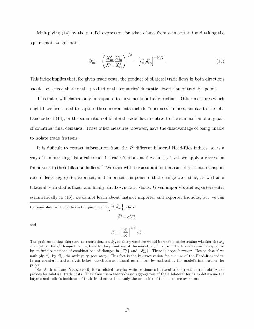
Multiplying (14) by the parallel expression for what i buys from n in sector j and taking the

square root, we generate:

�jni =

Xjni

Xjnn

Xjin

Xjii

!1=2=hdjnid

jin

i��j=2: (15)

This index implies that, for given trade costs, the product of bilateral trade �ows in both directions

should be a �xed share of the product of the countries�domestic absorption of tradable goods.

This index will change only in response to movements in trade frictions. Other measures which

might have been used to capture these movements include �openness� indices, similar to the left-

hand side of (14), or the summation of bilateral trade �ows relative to the summation of any pair

of countries��nal demands. These other measures, however, have the disadvantage of being unable

to isolate trade frictions.

It is di¢ cult to extract information from the I2 di¤erent bilateral Head-Ries indices, so as a

way of summarizing historical trends in trade frictions at the country level, we apply a regression

framework to these bilateral indices.12 We start with the assumption that each directional transport

cost re�ects aggregate, exporter, and importer components that change over time, as well as a

bilateral term that is �xed, and �nally an idiosyncratic shock. Given importers and exporters enter

symmetrically in (15), we cannot learn about distinct importer and exporter frictions, but we can

the same data with another set of parametersneSji ; edjnio where:

eSji = �jiSji ;and edjni = � �ji�jn

�1=�j edjni:The problem is that there are no restrictions on �ji , so this procedure would be unable to determine whether the d

jni

changed or the Sji changed. Going back to the primitives of the model, any change in trade shares can be explainedby an in�nite number of combinations of changes in

�T jiand

�djni. There is hope, however. Notice that if we

multiply djni by djin, the ambiguity goes away. This fact is the key motivation for our use of the Head-Ries index.

In our counterfactual analysis below, we obtain additional restrictions by confronting the model�s implications forprices.12See Anderson and Yotov (2009) for a related exercise which estimates bilateral trade frictions from observable

proxies for bilateral trade costs. They then use a theory-based aggregation of these bilateral terms to determine thebuyer�s and seller�s incidence of trade frictions and to study the evolution of this incidence over time.

17

extract their combined e¤ects by estimating the pooled regression for all i, n, and t:

ln�jni(t) = �jn(t) + �

ji (t) +

jni + "

jni(t). (16)

We do this separately for each manufacturing industry, j = D;N . Note that each regression

contains only N country dummy variables each period, any given observation will be in�uenced

by two of these country dummies. Again, each dummy represents the sum of the trade frictions

experienced by that country�s exporters and importers.

Figures 7 and 8 plot the four-quarter moving average of the country-time e¤ects �ji from a

weighted estimation of (16) for selected countries. We use a moving average due to the strong

seasonal e¤ects in the data. The coe¢ cients are normalized to zero in the �rst quarter of 2000 and

extend through the fourth quarter of 2009. The country-time e¤ects act proportionately on the

Head-Ries indices for all bilateral pairs involving any given country. For instance, if the series for

country i increases from 0 to 0.1, it implies that the index would increase 10 percent for all pairs

in which i is an exporter or an importer.

Looking at Figure 7, we see examples of countries where the recession did not bring with it

marked increases in trade frictions. Only a small share (or a negative share) of any declines in trade

�ows for Germany, the U.S., Mexico, and Italy should, according to this measure, be attributed to

declining trade frictions. Figure 8, by contrast, includes only countries for which there is a steep

increase in trade frictions (a decline in the index) during the recession. These countries include

Japan, China, Austria, and Finland, among others not shown. One important conclusion is that,

while there is evidence of increasing trade frictions in some countries, this shock appears to be

quite heterogenous across countries and is generally relatively muted. For some countries, in fact,

reduced trade frictions could have ameliorated the trade collapse.

5.4 Trade Frictions During the Great Depression

These results suggest there was not a large universal trade friction shock associated with the recent

recession. This should be interpreted as resulting from the data and not from any predisposition of

18

the calculation to attenuate an underlying increase in trade frictions. To con�rm that our measure

can pick up changes in trade frictions, we compare calculations made with data from the recent

recession to those using data from the Great Depression, a period with a major collapse in trade

that is widely believed to have re�ected, in part, increased trade barriers (see, for example, Irwin,

1998).

We have su¢ cient Depression-era data to construct Head-Ries indices (15) for the bilateral

trade between the United States and eight partners: Austria, Canada, Finland, Germany, Japan,

Spain, Sweden, and the United Kingdom. Appendix B includes the details on the data required for

this exercise. Figures 9 and 10 compare these Head-Ries indices from the Great Depression (seen

in the solid blue lines and corresponding to the lower x-axis) with the equivalent Head-Ries indices

from the recent recession (seen in the dotted red lines and corresponding to the upper x-axis).

Unlike our earlier analyses, these indices are calculated at the annual level and pool data from both

manufacturing sectors, to make an appropriate comparison.

Of the eight bilateral pairs, it just so happens that three of the countries, Austria, Finland, and

Japan, are among those displaying the largest declines of the Head-Ries indices in the recent period.

The declines for those three pairs for the recent recession are similar to the declines in the �rst

few years of the Great Depression. The other �ve countries show markedly larger Depression-era

drops, however, with average peak-to-trough declines in the Head-Ries index exceeding 50 percent,

compared to �at or increasing indices in the recent recession. In sum, the data we have on trade

and production in the Great Depression suggest that global Head-Ries indices dropped far more

broadly and more dramatically in the early 1930s than in the late 2000s.

6 Calibration

Having set up the model, discussed the four categories of shocks that can change trade �ows, and

given historical context on the path of these shocks, we now calibrate the model to perfectly match

the period from the �rst quarter of 2008 to the �rst quarter of 2009. The calibration exercise only

includes a balanced panel of countries for which we have good data on input-output structure,

19

production, and imports from and exports to all other included countries. After constructing

trade, production, GDP, de�cit, and input-output information for each country, and balancing this

panel, we are left with a dataset containing complete data for 22 countries responsible for about

75 percent of global manufacturing trade and global GDP.13 Table 1 lists the included countries,

shares in trade, and shares in global GDP, before and after the crisis, as well as a residual category

"rest of world."14

First, we re-formulate the model to facilitate computing its implications for changes in endoge-

nous variables. Next we describe how we parameterize the model for calculating changes.

6.1 Change Formulation

For any time-varying variable x in the model we denote its beginning-of-period or baseline value

as x and its end-of-period or counterfactual value as x0, with the �change� over the period (or

counterfactual change) denoted x = x0=x. We will take labor supply as �xed so that Y 0i = wiYi.

In terms of counterfactual levels and changes, the global input-output equations (12), for sectors

j 2 M and countries i = 1; 2; :::; I, become

�Xji

�0=�e�ji�0 (wiYi +D0i)� �ji �DSi �0 + X

l2M

e lji (1� e�li)"

IXn=1

��lni

�0 �X ln

�0#: (17)

The global market clearing conditions (13) become:

�XDi

�0+�XNi

�0 � hD0i � �DSi �0i = IXn=1

��Dni�0 �XDn

�0+

IXn=1

��Nni�0 �XNn

�0: (18)

The price equations (10) become:

pjn =

0@ IXi=1

�jniw��je�jii

�pji

��je jji (1�e�ji ) �pli

��je jli (1�e�ji ) djniAji

!��j1A�1=�j

; (19)

13These shares are highly similar before and after the crisis, suggesting we have a representative sample in termsof the declines in trade and output.14We use most countries for which we have high quality data, with the exceptions of Belgium and the Netherlands.

Belgium and the Netherlands are omitted because their manufacturing exports often exceed their manufacturingproduction (due to re-exports), and our framework is not capable of handling this situation.

20

where l 6= j is the other manufacturing sector. The trade share equations (11) become:

��jni

�0= �jniw

��je�jii

�pji

��je jji (1�e�ji ) �pli

��je jli (1�e�ji ) djniAji p

jn

!��j: (20)

Equations (17), (18), (19), and (20) determine the changes in endogenous variables implied by

a given set of shocks. We solve this set of equations for: (i) changes in wages wi, (ii) counterfactual

levels of spending (Xji )0, (iii) changes in prices pji , and (iv) counterfactual trade shares

��jni

�0for

countries i = 1; :::; I and sectors j 2 M . Baseline trade shares and GDPs are used to calibrate

the model. The forcing variables are the end-of-period or counterfactual demand shocks�e�ji�0 and

de�cits�DSi�0and D0i, changes in trade frictions d

jni, and changes in productivity A

ji .15

The system can be solved as follows. Given a vector of possible wage changes, (19) is solved

for price changes. Wage and price changes then imply counterfactual trade shares via (20). Given

counterfactual trade shares and wage changes, (17) can be solved as a linear system for counter-

factual levels of spending. If these levels of spending satisfy (18), then we have an equilibrium. If

not, we adjust wage changes according to where there is excess demand (with world GDP �xed)

and return to (19). Details are described in Appendix D.

Given the solution described above, we can use equation (8), as it applies to the counterfactual

levels: �Y ji

�0=

IXn=1

��jni

�0 �Xjn

�0; (21)

to obtain counterfactual levels of sectoral production and de�cits.

6.2 Parameter Values and Shocks

We start by setting �D = �N = 2. This value is between the smaller values typically used in the

open-economy macro literature and the larger values used in Eaton and Kortum (2002).

We have described above our procedure for backing out end-of period demand shocks (�ji )0. We

15As described in Appendix C, equilibrium outcomes for everything but price changes are invariant to productivity

shocks of a labor-augmenting form, i.e. Aji = �e�ji for some � > 0. Such shocks lead to price changes equal to 1=�.

Furthermore, shocks to service-sector productivity, given Aji , do not perturb the equilibrium outcomes. Either typeof productivity shock will likely alter welfare, but is irrelevant to the model�s implications for international trade.

21

use them to construct the demand shocks as they enter the model through equation (17):

�e�ji�0 = ��ji�0 + Sji (1� �Si )1� SSi (1� �Si )

��Si�0;

for j 2 M . End of period de�cits D0i and�DSi�0can be read directly from the data. They enter the

model via equations (17) and (18). Our residual country, "Rest of World," has its de�cit de�ned

such that the global de�cit equals zero.

We have described the Head-Ries index above. Calculating squared changes of it yields:

��jni

�2=�jni�

jin

�jnn�jii

=�djni

��j �djin

��j:

Here we need to decompose this measure to isolate�djni

��j. Dividing both sides of (20) by �jni we

get an expression for �jni. Dividing by the corresponding expression for �jii and rearranging yields:

�djni

��j=�jni�jii

pjipjn

!�j: (22)

We implement this equation using the changes in sectoral PPI�s we constructed earlier.16 We can

also retrieve productivity changes by rearranging (20) as it applies to n = i:

Aji =��jii

�1=�jwe�jii

�pji

�e jji (1�e�ji )�1 �pli

�e jli (1�e�ji ): (23)

The trade-friction and productivity shocks both enter the model through equation (19) and (20).17

We present cross-country evidence on these shocks, together with some of the underlying vari-

ables used to construct them, from the �rst quarter of 2008 to the �rst quarter of 2009. We begin

with the demand and de�cit shocks shown above as they varied over time within countries. The

16We estimate pjROW for j 2 M by simply averaging pji across the countries in our sample.17Price data, such as the PPI data we use here, are required to disentengle changes in productivity from changes

in trade frictions. As discussed in Appendix C, however, the combined impact of these two shocks on all non-pricevariables is robust to any procedure that separates them in an internally consistent way. For example, we can choosean arbitrary vector for the productivity shocks, back out the implied trade friction shocks, and other than prices,nothing in the model will change.

22

four panels in Figure 11 plot on the y-axis the changes in the durables and non-durables demand

shocks and the overall and non-manufacturing de�cits. The change in trade to GDP ratios during

the crisis are plotted along the x-axis. Figure 12 plots the corresponding changes in the durable

and non-durable productivity shocks, calculated according to equation (23), and changes in prices

in the two sectors (measured in U.S. dollars and relative to our numeraire of world GDP).

The trade-friction shocks, constructed according to equation (22), have both an importer and

exporter dimension. The two panels of Figure 13 contain histograms of the durable and non-durable

trade friction changes,�bdjni��j .18 The histograms exclude the largest and smallest 5 percentile

values (generally small country-pair outliers).

Table 2 lists the combined impact (on imports and exports relative to GDP) of all the shocks

associated with the recession, across all the countries used in our counterfactual exercises. By

construction, the combined e¤ect of our shocks fully accounts for the actual decline in trade from

the �rst quarter of 2008 to the �rst quarter of 2009. The top row of data in the table, in boldface

and labeled "World," shows that in global trade declined by 19 percent relative to GDP, with

durables dropping by 22 percent and non-durables dropping by 11 percent.

7 Counterfactuals

We now discuss our counterfactual exercises. Given values for the changes in the forcing variables

we solve (17), (18), (19), and (20), using an algorithm adapted from Dekle, Eaton, and Kortum

(2008). In the results that follow we treat all end-of-period de�cits (as a share of world GDP)

as exogenous, so that wage changes are endogenous. In future drafts we will consider a case of

exogenous wage changes and endogenous end-of-period manufacturing de�cits.

It will be convenient to de�ne the set of all shocks:

�0 =nnb�Di o ;nb�Ni o ;n bDio ;n bDSi o ;nbdDnio ;nbdNnio ;n bADi o ;n bASi oo ;

18To back out the implied change in the trade friction itself, these changes should be divided by �j = 2.

23

for all countries i; n 2 I.19 For any given four-quarter period and any given set of shocks �, we

can solve our model to generate changes in all values and �ows in the global system relative to the

base period. As an example, consider the case where we choose the �rst quarter of 2008 as the base

period. If we solve the model with all shocks in �0 equal to one, implying the shocks did not change

at all relative to this base period, the model would generate outcome variables (such as production,

trade, GDP, etc.) precisely equal to those seen in the �rst quarter of 2008, as if the recession and

the shocks that generated it never occurred. If, on the other hand, we solve the model with the set

of shocks �0 = data, where "data" means that the shock values are those for 2008:Q1 to 2009:Q1

as given in the previous tables and plots, the model would generate values precisely equal to those

seen in the �rst quarter of 2009. It will be convenient to de�ne these two special cases of the shock

matrices as �08Q1 and �09Q1, respectively.

7.1 Accounting the Trade Decline from 2006-2009

We start by considering a series of four-quarter changes, beginning with the period from 2006:Q1

to 2007:Q1 all the way through to the period from 2008:Q4 to 2009:Q4. We run the model for

each of these 12 four-quarter periods under various counterfactual assumptions and consider the

implications at the global level. For instance, when we run the simulation after inputting all

observed shocks, the counterfactual in each period shows the actual gross percentage change in

world trade/GDP over the previous four quarters, as would be found in the raw data. Figure 14

plots these results as the boldfaced black line labeled "Data." (The 12 overlapping four-quarter

changes are plotted as a continuous line, but it should be remembered that each calculation is done

independently of those that came before. The changes are not cumulative.)

One sees that after mild rates of growth in the periods ending in 2007, global manufacturing

trade/GDP was essentially unchanged until the fourth quarter of 2008, when it dropped nearly 10

percent relative to its value four quarters earlier. The drop continued and world trade/GDP in

the �rst and second quarters of 2009 were about 20 percent below its respective levels in the �rst

19We note that while we write bDSi and bDi, we really only need information on

�DSi

�0and D0

i, and so do not run

into problems if bDSi and bDi are unde�ned because initial de�cits are zero.

24

and second quarters of 2008. By the end of the dataset, annual growth in global trade/GDP had

�attened, as represented by the black line approaching the value 1.0. We expect the line to exceed

one in future quarters as trade levels recover.

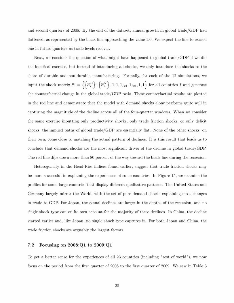
Next, we consider the question of what might have happened to global trade/GDP if we did

the identical exercise, but instead of introducing all shocks, we only introduce the shocks to the

share of durable and non-durable manufacturing. Formally, for each of the 12 simulations, we

input the shock matrix �0 =nnb�Di o ;nb�Ni o ; 1; 1; 1Ix1; 1Ix1; 1; 1o for all countries I and generate

the counterfactual change in the global trade/GDP ratio. These counterfactual results are plotted

in the red line and demonstrate that the model with demand shocks alone performs quite well in

capturing the magnitude of the decline across all of the four-quarter windows. When we consider

the same exercise inputting only productivity shocks, only trade friction shocks, or only de�cit

shocks, the implied paths of global trade/GDP are essentially �at. None of the other shocks, on

their own, come close to matching the actual pattern of declines. It is this result that leads us to

conclude that demand shocks are the most signi�cant driver of the decline in global trade/GDP.

The red line dips down more than 80 percent of the way toward the black line during the recession.

Heterogeneity in the Head-Ries indices found earlier, suggest that trade friction shocks may

be more successful in explaining the experiences of some countries. In Figure 15, we examine the

pro�les for some large countries that display di¤erent qualitative patterns. The United States and

Germany largely mirror the World, with the set of pure demand shocks explaining most changes

in trade to GDP. For Japan, the actual declines are larger in the depths of the recession, and no

single shock type can on its own account for the majority of these declines. In China, the decline

started earlier and, like Japan, no single shock type captures it. For both Japan and China, the

trade friction shocks are arguably the largest factors.

7.2 Focusing on 2008:Q1 to 2009:Q1

To get a better sense for the experiences of all 23 countries (including "rest of world"), we now

focus on the period from the �rst quarter of 2008 to the �rst quarter of 2009. We saw in Table 3

25

that world trade dropped 19 percent relative to economic activity over this period. Compared to

this 19 percent, Table 3 shows that a 15 percent decline is generated from a counterfactual recession

in which manufacturing demand dropped as it did but with no other shocks. Table 4 shows that

a counterfactual recession in which the only change is the shock to trade frictions produces only

a 1 percent decline in global trade. In addition to these aggregate results, Tables 2 through 4 list

separately the experiences of each country in the data, in the counterfactual with only demand

shocks, and in the counterfactual with only trade friction shocks.

We now introduce a measure to summarize the ability of our counterfactuals to match the cross-

country pattern. We write the gross change in any particular outcome variable � for country i as

b�i(�0) = �0i=�08Q1i to represent its value when the system is solved using the set of shocks �0 relative

to the value that was observed in the �rst quarter of 2008. For example, if �i is country i�s overall

trade to GDP ratio, then b�i(�09Q1) is the gross percentage change in trade to GDP observed from2008:Q1 to 2009:Q1 in that country. (Note that with this base period, b�i(�08) = 1 for any variable�i, by de�nition.)

We construct the following measure:

��0�=

IXi

wi

�b�i ��0�� b�i ��09Q1��2 :It is a weighted sum of squared deviations of the vector b� (�0) from the vector b� ��09Q1�, with eachelement�s deviation weighted by wi, with

Piwi = 1. An important feature of this measure is that

it does not net out the mean value of the deviation. For instance, if � is the trade to GDP ratio,

then ��08Q1

�measures total squared changes across countries in trade to GDP ratios during the

recession. To measure the share of these total changes in � over the recession that are captured by

a set of shocks �0, we de�ne:

V��0�=1� � (�0)

� (�08Q1):

Imagine running a counterfactual scenario with all shocks equal to 1, except for changes in

countries�non-manufacturing trade de�cits, which are set equal to what was observed in the data.

26

The scenario would generate a counterfactual vector of changes in trade to GDP ratios. The x-

axis in the top-left plot of Figure 16 plots the vector b� ��09Q1�, while the y-axis plots the vectorb� (�0).20 If all the points were on the 45 degree line, it would indicate that the observed changes inthe non-manufacturing de�cits alone can fully explain the cross-country changes in trade to GDP

during that four-quarter period. In such a case, V (�0) would equal 1. As is easy to see, however,

this counterfactual was far from aligning the points along the 45 degree line. Using shares of pre-

recession global trade as our weights (wi), we calculate V (�0) = 0:05. Thus, the subtitle of the

top-left plot of Figure 16 says "Share of Trade-Weighted Variance Explained: 5%," and we conclude

that the non-manufacturing de�cit shocks can explain very little of the pattern of trade changes in

the recession.21

The other three plots in Figure 16 show results from counterfactual scenarios simulated with

both trade friction shocks, with durable manufacturing shocks, and with all shocks included. The

top-right plot, capturing trade frictions, explains a bit more of the cross-country pattern than did

non-manufacturing de�cits. The share of trade-weighted variance explained is listed as 9 to 17

percent, where the upper bound of this range is generated from adding all trade frictions except

those estimated with the "Rest of World," since those measurements involve more assumptions

and less raw data than the others. The most notable result is the durable demand shock on the

bottom-left panel of Figure 16. Durable demand shocks, on their own, explain 64 percent of the

trade-weighted variance. Finally, as shown in the bottom-right panel of Figure 16, when all shocks

are implemented, they perfectly explain changes in the economic system. This result is, of course,

true by construction.

Table 5 lists the shares of trade-weighted variance explained by various shock combinations, in-

cluding those displayed in Figure 16. Those combinations that include trade frictions list a range,

where the larger value assumes no change in trade frictions with the "rest of the world." The contri-

butions of each shock are not orthogonal to the others and hence, the shares of variance explained

by each shock will not sum to one. Given these shocks may not be introduced independently in

20The plots actually show the net rates of change, that is, b� (�)� 1.21Note that this calculation can very well be negative. We would expect this with any shock that pushes the vector

of outcome variables even further away from the post-recession data.

27

some recessions, it is useful to observe that the only combinations the generate very large contribu-

tions involve durable demand shocks. Further, adding productivity or de�cit shocks to the demand

shocks increases their explanatory power only slightly. Hence, though one might prefer to consider

counterfactuals using combinations of these shocks, the demand shocks remain the most important

proximate driver of changes in the pattern of trade/GDP.

7.3 Other Counterfactuals

Given the heterogeneity in the shocks a¤ecting countries in the recent recession, we also consider

counterfactuals run at the country- or region-level. As an example, imagine one wants to know

the global impact of the decline in durables demand just in the U.S. The top panel of Table 6

shows simulated trade �ows at the country and global level (for selected countries) when the only

shock we introduce into the system is b�DUS . The impact of this single shock on the world is large�it reduces global durables trade by about 3 percent relative to GDP. One also notes the impact

of geography. Mexico and Canada are a¤ected very signi�cantly, while Germany, for example, is

relatively insulated.

The bottom panel of Table 6 shows an alternative exercise where the only shocks introduced

are the changes in trade frictions observed in China and Japan. These reduce total global trade by

about 3 percent relative to GDP, but also have interesting cross-country implications. For example,

the counterfactual produces trade diversion as manifest in the increase in South Korea�s trade to

GDP ratio.

8 Conclusion

A prominent characteristic of the recent global recession was a large and rapid drop in trade relative

to GDP. Motivated by these dramatic changes in the cross-country pattern of trade, production,

and GDP, we build an accounting framework relating them to shocks to demand, trade frictions,

de�cits, and productivities across several sectors. Applying our framework to the recent recession,

we �nd that the bulk of the decline in trade/GDP can be explained by the shocks to manufacturing

28

demand, with a particularly important role for the shocks to durable manufacturing demand. The

trade declines in China and Japan, however, re�ect a moderate contribution from increased trade

frictions.

We developed this approach with the recent recession in mind. We anticipate, however, that

the framework can be applied quite generally to study the geography of global booms and busts.

29

References

[1] Alessandria, George, Joseph Kaboski, and Virgiliu Midrigan. "Inventories, Lumpy Trade, andLarge Devaluations," Working Paper, 2009.

[2] Alessandria, George, Joseph Kaboski, and Virgiliu Midrigan. "The Great Trade Collapse of2008-09: An Inventory Adjustment?" Working Paper, 2010.

[3] Alvarez, Fernando and Robert E. Lucas. �General Equilibrium Analysis of the Eaton-KortumModel of International Trade,�Journal of Monetary Economics, September 2007, 54: 1726-1768.

[4] Amiti, Mary and David Weinstein. "Exports and Financial Shocks," Working Paper, 2009.

[5] Anderson, James E. and Eric van Wincoop. �Gravity with Gravitas: A Solution to the BorderPuzzle,�American Economic Review, March 2003, 93: 170-192.

[6] Anderson, James E. and Yoto Yotov. "The Changing Incidence of Geography," Working Paper,2009.

[7] Arkolakis, Costas, Arnaud Costinot, and Andres Rodriguez-Clare. "New Trade Models, SameOld Gains?" Working Paper, 2009.

[8] Baldwin, Richard. Vox EU Ebook, 2009.

[9] Bems, Rudolphs, Johnson, Robert, and Kei-Mu Yi. "The Role of Vertical Linkages in thePropagation of the Global Downturn of 2008," Working Paper, 2010.

[10] Berman, Nicolas and Philippe Martin. "The Vulnerability of Sub-Saharan Africa to the FinancialCrisis: The Case of Trade," Working Paper, 2009.

[11] Bhagwati, Jagdish. Comments in "Collapse in World Trade: A Symposium of Views," The Interna-tional Economy, Spring 2009.

[12] Brock, William. Comments in "Collapse in World Trade: A Symposium of Views," The InternationalEconomy, Spring 2009.

[13] Bundesamt fur Statistik. Statistisches Handbuch fur die Republik Osterreich. Vienna: Bundesamtesfur Statistik, 1927-1936.

[14] Caliendo, Lorenzo and Fernando Parro. "Estimates of the Trade and Welfare E¤ects of NAFTA,"Working Paper, 2009.

[15] Carter, Susan B., Scott Sigmund Gartner, Michael R. Haines, Alan L. Olmstead, RichardSutch, and Gavin Wright. Historical Statistics of the United States: Millenial Edition, Vol. 4. Cam-bridge: Cambridge University Press, 2006.

[16] Chaney, Thomas. �Distorted Gravity: Heterogeneous Firms, Market Structure, and the Geographyof International Trade,�American Economic Review, September 2008, 98: 1707-1721.

[17] Chari, V.V., Patrick Kehoe, and Ellen McGrattan. "Business Cycle Accounting," Econometrica,May 2007, 75, pp. 781-836.

[18] Chow, G. and A. Lin. "Best Linear Unbiased Interpolation, Distribution and Extrapolation of TimeSeries by Related Series," Review of Economics and Statistics, 1971.

[19] Dekle, Robert, Jonathan Eaton, and Samuel Kortum. �Unbalance Trade,�American EconomicReview: Papers and Proceedings, May 2007, 97: 351-355.

30

[20] Dekle, Robert, Jonathan Eaton, and Samuel Kortum. �Global Rebalancing with Gravity: Mea-suring the Burden of Adjustment,�IMF Sta¤ Papers, Vol. 55, No 3:511-540.

[21] Denton, F.T. "Adjustment of Monthly or Quarterly Series to Annual Totals: An Approach Based onQuadratic Minimization," Journal of the American Statistical Association," 1971, 66: 99-102.

[22] Di Fonzo, Tommaso. "Temporal Disaggregation of Economic Time Series: Towards a Dynamic Ex-tension," Working Paper, 2002.

[23] Eaton, Jonathan and Samuel Kortum. �Technology, Geography, and Trade,�Econometrica, Sep-tember 2002, 70, pp. 1741-1780.

[24] Eichengreen, Barry. Comments in "Collapse in World Trade: A Symposium of Views," The Interna-tional Economy, Spring 2009.

[25] Engel, Charles and Jian Wang. �International Trade in Durable Goods: Understanding Volatility,Cyclicality, and Elasticities,�Working Paper, 2009.

[26] Feenstra, Robert and Chang Hong. "China�s Exports and Employment," Working Paper, 2007.

[27] Fernandez, Roque. "A Methodological Note on the Estimation of Time Series," The Review of Eco-nomics and Statistics, 1981, Vol. 63, No. 3, pp471-476.

[28] Friedman, Milton. "The Interpolation of Time Series by Related Series," Journal of the AmericanStatistical Association, 1962, 57: pp729-757.

[29] Head, Keith and John Ries. "Increasing Returns versus National Product Di¤erentiation as anExplanation for the Pattern of U.S.-Canada Trade," American Economic Review, September 2001, 91:858-876.

[30] Irwin, Douglas A.. "The Smoot-Hawley Tari¤: A Quantitative Assessment," Review of Economicsand Statistics, May 1998, 80: pp326-334.

[31] Jacks, Meissner, and Novy. "Trade Booms, Trade Busts, and Trade Costs," Working Paper, 2009.

[32] Johnson, Robert and Guillermo Noguera. "Accounting for Intermediates: Production Sharing andTrade in Value Added," Working Paper, 2009.

[33] McKinnon, Ronald. Comments in "Collapse in World Trade: A Symposium of Views," The Interna-tional Economy, Spring 2009.

[34] Melitz, Marc. �The Impact of Trade on Aggregate Industry Productivity and Intra-Industry Reallo-cations,�Econometrica November 2003.

[35] Ministerio de Hacienda y Comercio. Extracto Estadistico del Peru 1939. Imprenta Americana:Lima, Peru. 1939.

[36] Urquhart, M.C. (ed.). Historical Statistics of Canada. Ottawa, Canada: Statistics Canada, 1983.

[37] Redding, Stephen and Anthony Venables. �Economic Geography and International Inequality,�Journal of International Economics, January 2004, 62, pp. 53-82.

[38] Smits, J.P, P.J. Woltjer, and D. Ma. "A Dataset on Comparative Historical National Accounts, ca.1970-1950: A Time-Series Perspective," Groningen Growth and Development Centre Research Memo-randum GD-107, Groningen: University of Groningen. 2009.

[39] Statistischen Reichsamt. Statistisches Jahrbuch fur das Deutsche Reich. Berlin: Reimer Hobbing,1931, 1935, 1940.

31

[40] U.K. Board of Trade. Statistical Abstract for the United Kingdom: 1924:1938. London: StatisticalDepartment, Board of Trade, 1938.

[41] U.S. Department of Commerce. Foreign Commerce Yearbook, Vols. 1928-1938. New York: Green-wood Press, 1968.

[42] Waugh, Michael. "Bilateral Trade, Relative Prices, and Trade Costs," Working Paper, 2007.

[43] Yi, Kei-Mu. "The Collapse of Global Trade: The Role of Vertical Specialisation." In The Collapse ofGlobal Trade, Murky Protectionism, and the Crisis: Recommendations for the G20, edited by RichardBaldwin and Simon Evenett, 2009.

32

Tables

Coun

try

2008

:Q1

2009

:Q1

2008

:Q1

2009

:Q1

2008

:Q1

2009

:Q1

Aus

tria

0.7

0.7

1.7

1.5

1.5

1.5

Cana

da2.

62.

32.

72.

53.

13.

3Ch

ina

6.6

8.1

12.2

13.6

7.0

7.1

Czec

h Re

publ

ic0.

40.

31.

31.

21.

21.

1D

enm

ark

0.6

0.5

0.9

0.9

0.9

0.9

Finl

and

0.5

0.4

0.9

0.7

0.7

0.6

Fran

ce4.

94.

75.

25.

15.

35.

6G

erm

any

6.3

5.8

13.1

12.7

8.9

9.4

Gre

ece

0.6

0.6

0.2

0.2

0.6

0.7

Hun

gary

0.3

0.2

1.0

0.9

0.9

0.8

Indi

a2.

22.

11.

11.

31.

41.

7It

aly

3.9

3.7

4.7

4.4

3.9

3.7

Japa

n8.

29.

57.

05.

73.

94.

2M

exic

o1.

91.

52.

12.

32.

42.

5Po

land

0.9

0.7

1.5

1.4

1.6

1.4

Rom

ania

0.3

0.3

0.4

0.4

0.7

0.6

Slov

akia

0.1

0.2

0.6

0.6

0.6

0.6

Sout

h Ko

rea

1.8

1.3

3.5

3.7

2.5

2.4

Spai

n2.

72.

62.

32.

13.

22.

6Sw

eden

0.8

0.7

1.6

1.4

1.3

1.2

Uni

ted

King

dom

4.8

3.8

3.7

3.5

5.0

4.7

Uni

ted

Stat

es23

.926

.69.

910

.914

.014

.7Re

st o

f Wor

ld25

.123

.322

.622

.929

.528

.7

Shar

e of

Glo

bal G

DP

in U

SD (P

erce

nt)

Shar

e of

Glo

bal I

mpo

rts

(Per

cent

)Sh

are

of G

loba

l Exp

orts

(Per

cent

)

Table1:CountryCoverageinData

Notes:

33

NoRecession

Shocks: None

All Vars All DurablesNon

Durables All DurablesNon

Durables

World 1.00 0.81 0.78 0.89 0.81 0.78 0.89

Austria 1.00 0.78 0.73 0.89 0.84 0.80 0.92Canada 1.00 0.89 0.83 1.03 0.99 0.93 1.14China 1.00 0.74 0.72 0.79 0.67 0.67 0.68Czech Republic 1.00 0.80 0.79 0.87 0.80 0.76 0.90Denmark 1.00 0.90 0.84 0.97 0.89 0.86 0.94Finland 1.00 0.72 0.69 0.79 0.77 0.72 0.91France 1.00 0.83 0.79 0.89 0.88 0.85 0.94Germany 1.00 0.85 0.81 0.95 0.92 0.89 0.99Greece 1.00 0.84 0.75 0.91 0.91 0.88 0.94Hungary 1.00 0.86 0.83 0.99 0.84 0.80 0.96India 1.00 1.02 1.13 0.90 1.05 1.05 1.04Italy 1.00 0.81 0.78 0.88 0.82 0.76 0.93Japan 1.00 0.57 0.56 0.66 0.76 0.68 0.91Mexico 1.00 1.05 1.03 1.19 1.02 1.01 1.03Poland 1.00 0.93 0.90 1.00 0.87 0.82 0.96Romania 1.00 0.92 0.93 0.90 0.78 0.67 0.99Slovakia 1.00 0.75 0.74 0.80 0.77 0.72 0.91South Korea 1.00 1.15 1.16 1.11 1.03 1.02 1.05Spain 1.00 0.76 0.70 0.86 0.70 0.63 0.83Sweden 1.00 0.86 0.79 1.04 0.89 0.82 1.05United Kingdom 1.00 0.98 0.90 1.14 0.98 0.90 1.14United States 1.00 0.81 0.79 0.84 0.77 0.73 0.87Rest of World 1.00 0.88 0.82 0.98 0.85 0.83 0.92

Exports / GDP Imports / GDP

Recession (2008:Q1 to 2009:Q1)

All Shocks Introduced

Table 2: Imports/GDP and Exports/GDP over RecessionNotes: All variables expressed relative to global GDP. Calculations using � = 1 restricted interpolationsand extrapolations.

34

NoRecession

Shocks: None



Durables

World 1.00 0.85 0.82 0.92 0.85 0.82 0.92


Demand Shocks Only

Durable and NonDurable Demand Shocks Introduced


Table 3: Counterfactual Results with Demand Shocks OnlyNotes: �D = �N = 2: All variables expressed relative to global GDP. Calculations using � = 1 restrictedinterpolations and extrapolations.

35

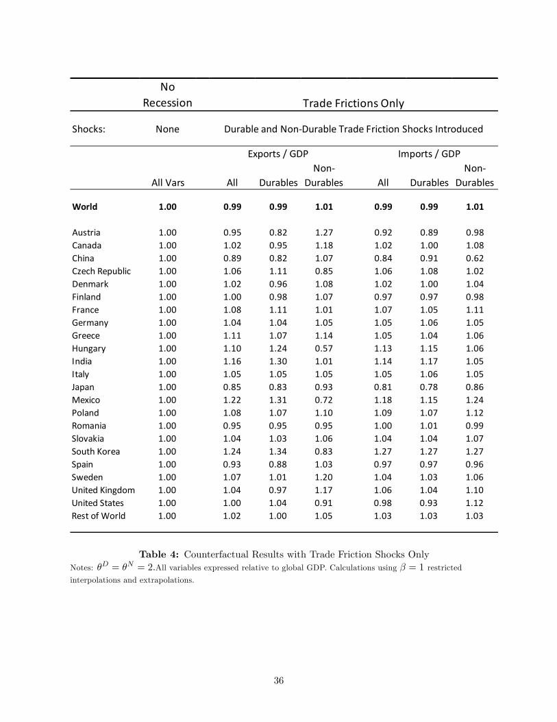
NoRecession

Shocks: None



Durables

World 1.00 0.99 0.99 1.01 0.99 0.99 1.01


Trade Frictions Only

Durable and NonDurable Trade Friction Shocks Introduced


Table 4: Counterfactual Results with Trade Friction Shocks OnlyNotes: �D = �N = 2:All variables expressed relative to global GDP. Calculations using � = 1 restrictedinterpolations and extrapolations.

36

Table5:Cross-SectionalExplanatoryPowerofCombinationsofShocks,2008:Q1to2009:Q1

Notes:�D=�N

=2:

37

NoRecession

Shocks: None



Durables

World 1.00 0.98 0.97 1.00 0.98 0.97 1.00

Canada 1.00 0.97 0.92 1.07 0.98 0.97 0.98China 1.00 1.00 0.99 1.03 0.99 0.99 0.99Germany 1.00 1.00 1.00 1.01 1.00 1.00 1.00Japan 1.00 1.00 0.99 1.03 0.98 0.98 0.99Mexico 1.00 0.96 0.94 1.09 0.97 0.97 0.96South Korea 1.00 1.00 0.99 1.02 0.99 0.99 0.99United Kingdom 1.00 0.99 0.99 1.01 1.00 1.00 1.00United States 1.00 0.89 0.89 0.88 0.91 0.85 1.05Rest of World 1.00 0.99 0.98 1.02 1.00 0.99 1.00

Only U.S. Durables Demand Shock

Durable Demand Shock for U.S. Introduced


NoRecession

Shocks: None



Durables

World 1.00 0.97 0.97 0.97 0.97 0.97 0.97

Canada 1.00 1.01 1.03 0.97 1.01 1.01 1.02China 1.00 0.87 0.81 1.04 0.83 0.90 0.61Germany 1.00 1.01 1.02 0.99 1.01 1.01 1.01Japan 1.00 0.84 0.83 0.93 0.82 0.79 0.88Mexico 1.00 1.03 1.04 0.95 1.02 1.02 1.03South Korea 1.00 1.12 1.15 0.96 1.13 1.13 1.15United Kingdom 1.00 1.01 1.02 1.00 1.01 1.01 1.02United States 1.00 0.96 0.98 0.93 0.98 0.95 1.03Rest of World 1.00 0.97 0.98 0.97 0.99 0.98 1.00

Only Trade Friction Shocks in China and Japan

Both Trade Frictions Shocks in China and Japan


Table 6: Country/Region-speci�c CounterfactualsNotes: �D = �N = 2:All variables expressed relative to global GDP. Calculations using � = 1 restrictedinterpolations and extrapolations.

38

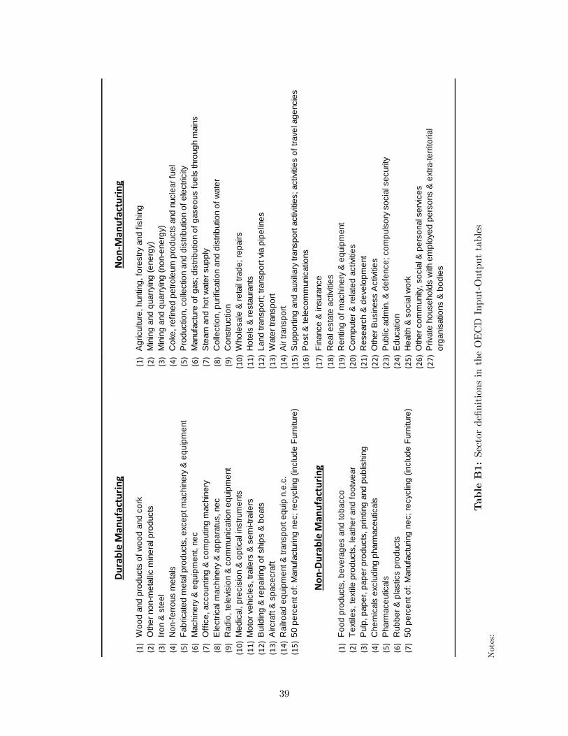
(1)

Woo

d an

d pr

oduc

ts o

f woo

d an

d co

rk(1

)A

gric

ultu

re, h

untin

g, fo

rest

ry a

nd fi

shin

g(2

)O

ther

non

met

allic

min

eral

pro

duct

s(2

)M

inin

g an

d qu

arry

ing

(ene

rgy)

(3)

Iron

& s

teel

(3)

Min

ing

and

quar

ryin

g (n

one

nerg

y)(4

)N

onfe

rrous

met

als

(4)

Cok

e, re

fined

pet

role

um p

rodu

cts

and

nucl

ear f

uel

(5)

Fabr

icat

ed m

etal

pro

duct

s, e

xcep

t mac

hine

ry &

equ

ipm

ent

(5)

Pro

duct

ion,

col

lect

ion

and

dist

ribut

ion

of e

lect

ricity

(6)

Mac

hine

ry &

equ

ipm

ent,

nec

(6)

Man

ufac

ture

of g

as; d

istri

butio

n of

gas

eous

fuel

s th

roug

h m

ains

(7)

Offi

ce, a

ccou

ntin

g &

com

putin

g m

achi

nery

(7)

Ste

am a

nd h

ot w

ater

sup

ply

(8)

Ele

ctric

al m

achi

nery

& a

ppar

atus

, nec

(8)

Col

lect

ion,

pur

ifica

tion

and

dist

ribut

ion

of w

ater

(9)

Rad

io, t

elev

isio

n &

com

mun

icat

ion

equi

pmen

t(9

)C

onst

ruct

ion

(10)

Med

ical

, pre

cisi

on &

opt

ical

inst

rum

ents

(10)

Who

lesa

le &

reta

il tra

de; r

epai

rs(1

1)M

otor

veh

icle

s, tr

aile

rs &

sem

itra

ilers

(11)

Hot

els

& re

stau

rant

s(1

2)B

uild

ing

& re

pairi

ng o

f shi

ps &

boa

ts(1

2)La

nd tr

ansp

ort;

trans

port

via

pipe

lines

(13)

Airc

raft

& s

pace

craf

t(1

3)W

ater

tran

spor

t(1

4)R

ailro

ad e

quip

men

t & tr

ansp

ort e

quip

n.e

.c.

(14)

Air

trans

port

(15)

50 p

erce

nt o

f: M

anuf

actu

ring

nec;

recy

clin

g (in

clud

e Fu

rnitu

re)

(15)

Sup

porti

ng a

nd a

uxilia

ry tr

ansp

ort a

ctiv

ities

; act

iviti

es o

f tra

vel a

genc

ies

(16)

Pos

t & te

leco

mm

unic

atio

ns(1

7)Fi

nanc

e &

insu

ranc

e(1

8)R

eal e

stat

e ac

tiviti

es(1

)Fo

od p

rodu

cts,

bev

erag

es a

nd to

bacc

o(1

9)R

entin

g of

mac

hine

ry &

equ

ipm

ent

(2)

Text

iles,

text

ile p

rodu

cts,

leat

her a

nd fo

otw

ear

(20)

Com

pute

r & re

late

d ac

tiviti

es(3

)P

ulp,

pap

er, p

aper

pro

duct

s, p

rintin

g an

d pu

blis

hing

(21)

Res

earc

h &

dev

elop

men

t(4

)C

hem

ical

s ex

clud

ing

phar

mac

eutic

als

(22)

Oth

er B

usin

ess

Act

iviti

es(5

)P

harm

aceu

tical

s(2

3)P

ublic

adm

in. &

def

ence

; com

puls

ory

soci

al s

ecur

ity(6

)R

ubbe

r & p

last

ics

prod

ucts

(24)

Edu

catio

n(7

)50

per

cent

of:

Man

ufac

turin

g ne

c; re

cycl

ing

(incl

ude

Furn

iture

)(2

5)H

ealth

& s

ocia

l wor

k(2

6)O

ther

com

mun

ity, s

ocia

l & p

erso

nal s

ervi

ces

(27)

Priv

ate

hous

ehol

ds w

ith e

mpl

oyed

per

sons

& e

xtra

terri

toria

lor

gani

satio

ns &

bod

ies

Dur

able

Man

ufac

turi

ngN

onM

anuf

actu

ring

Non

Dur

able

Man

ufac

turi

ng

TableB1:Sectorde�nitionsintheOECDInput-Outputtables

Notes:

39

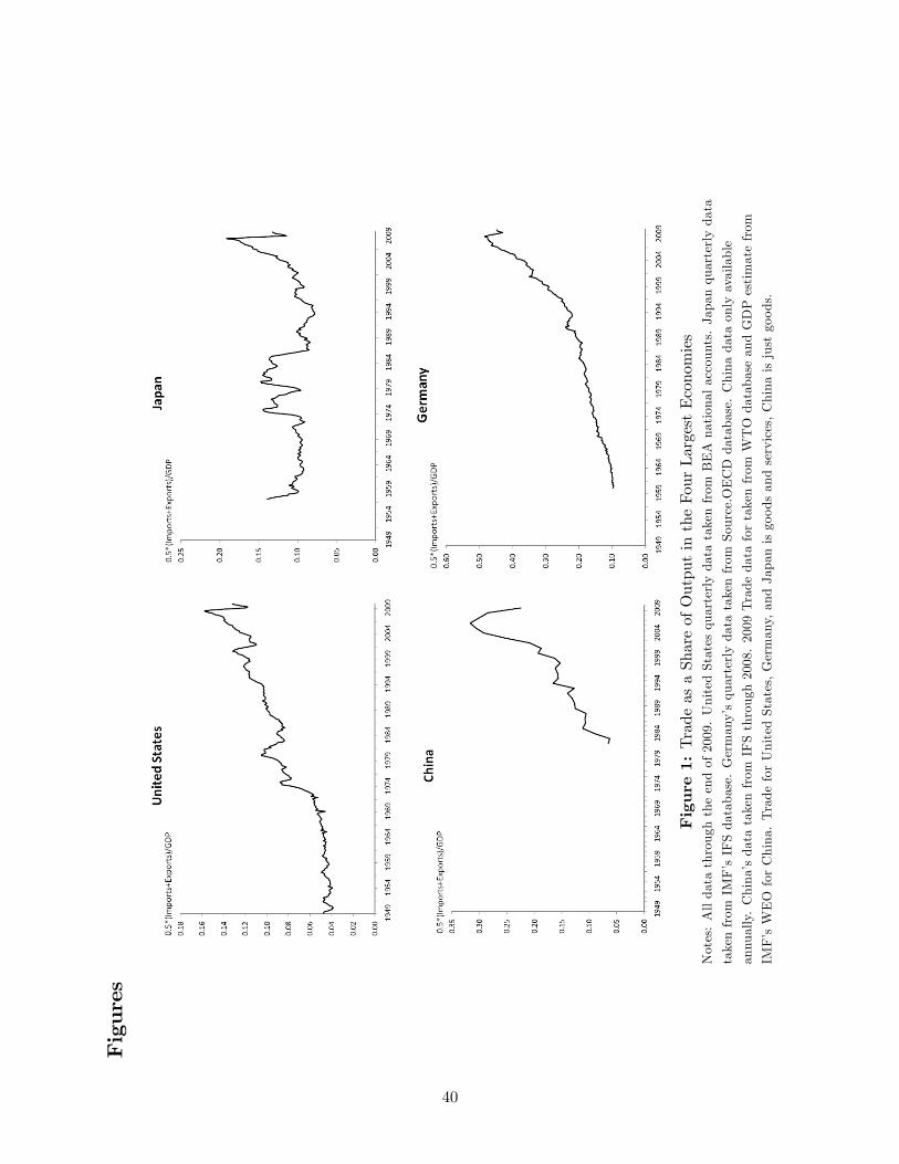
Figures

Figure1:TradeasaShareofOutputintheFourLargestEconomies

Notes:Alldatathroughtheendof2009.UnitedStatesquarterlydatatakenfrom

BEAnationalaccounts.Japanquarterlydata

takenfrom

IMF�sIFSdatabase.Germany�squarterlydatatakenfrom

Source.OECDdatabase.Chinadataonlyavailable

annually.China�sdatatakenfrom

IFSthrough2008.2009Tradedatafortakenfrom

WTOdatabaseandGDPestimatefrom

IMF�sWEOforChina.TradeforUnitedStates,Germany,andJapanisgoodsandservices,Chinaisjustgoods.

40

Figure2:TheCyclicalPropertiesofTradable-SectorActivityandTradeinU.S.andJapan

Notes:FortheU.S.,manufacturingspendingisthesumofnon-farm

non-�nancialbusinesscapitalspending,personalconsumptionexpendituresondurables,

andhalfofpersonalconsumptionexpendituresonnon-durables(onlyhalfbecauseitincludessomenon-manufacturesandservices).Non-oilimportsaretotal

importslessimportsofpetroleum

andpetroleum

products.ForJapan,manufacturingspendingisthesumofbusinessexpenditureonnewplantandequipment,

householdexpenditureondurablegoods,andhouseholdexpenditureonsemi-durables.Non-oilimportsaretotalimportslessimportsofcrudeandpartly

re�nedpetroleum.Allseriesarefrom

Datastream.

41

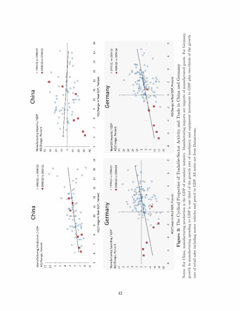
Figure3:TheCyclicalPropertiesofTradable-SectorActivityandTradeinChinaandGermany

Notes:ForChina,manufacturingproductionistheGDPofsecondaryindustry.Manufacturingimportsareimportsofmanufacturedgoods.ForGermany,

growthinmanufacturingspendingtoGDPisonethirdofthegrowthrateofmachineryandequipmentinvestmenttoGDPplustwo-thirdsofthegrowth

rateofretailsalesincludingmotorvehiclesandpetroltoGDP.Allseriesarefrom

Datastream.

42

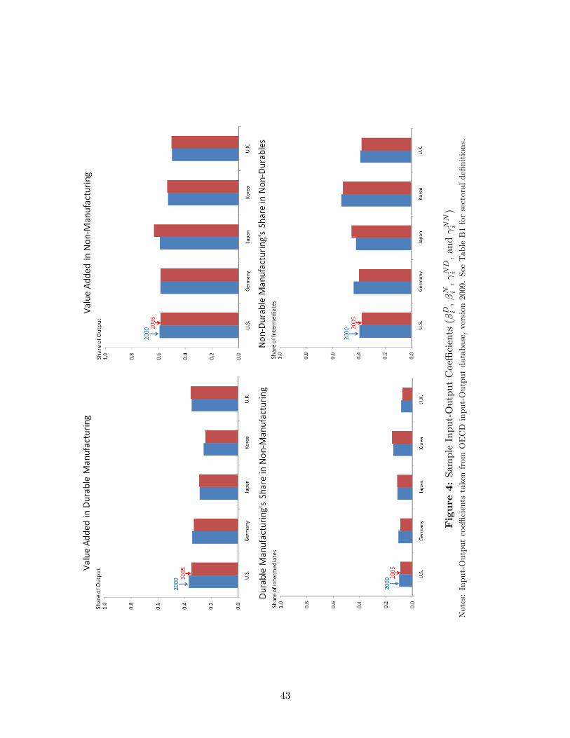
Figure4:SampleInput-OutputCoe¢cients(�D i,�N i, ND

i,and NN

i)

Notes:Input-Outputcoe¢cientstakenfrom

OECDinput-Outputdatabase,version2009.SeeTableB1forsectoralde�nitions.

43

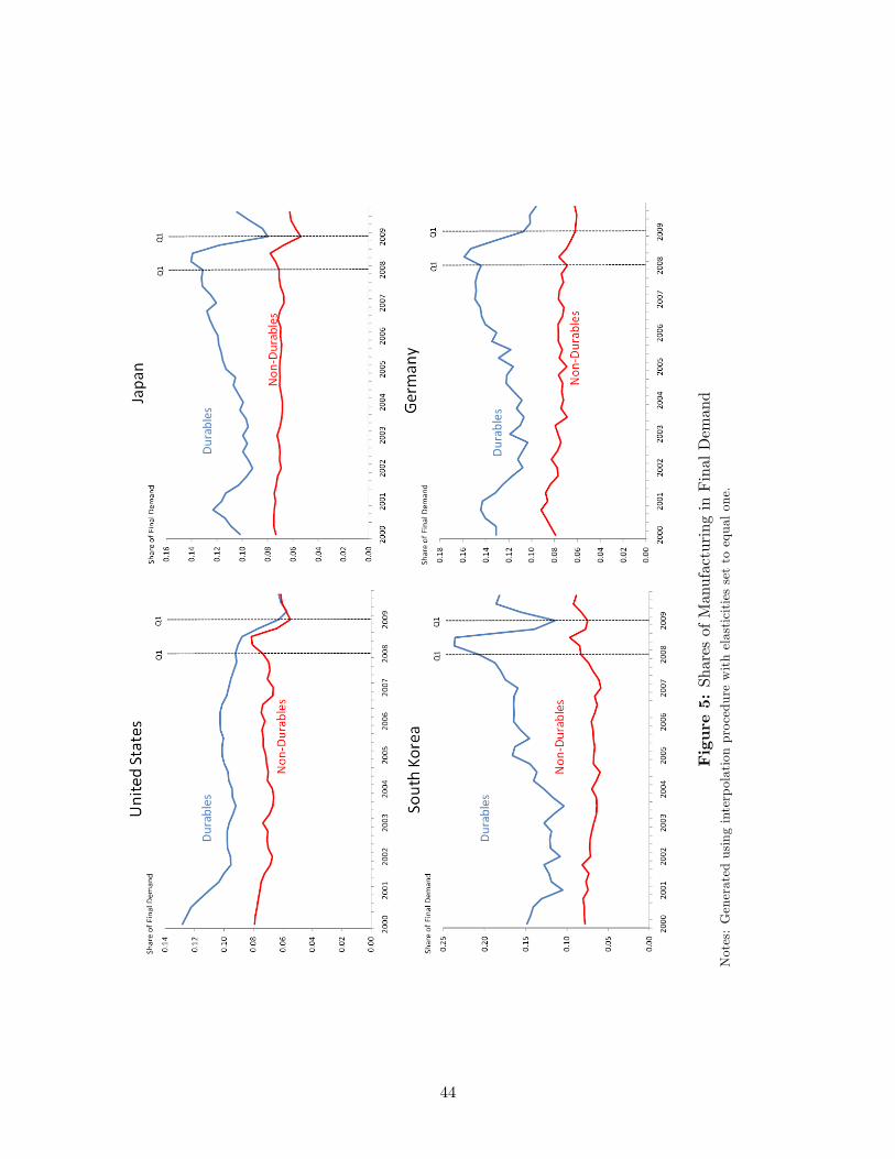
Figure5:SharesofManufacturinginFinalDemand

Notes:Generatedusinginterpolationprocedurewithelasticitiessettoequalone.

44

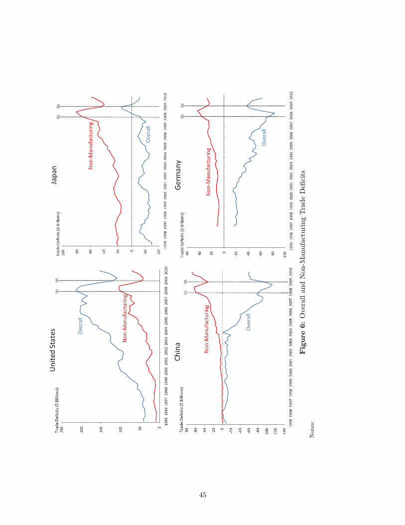
Figure6:OverallandNon-ManufacturingTradeDe�cits

Notes:

45

Figure7:CountrieswithoutLargeNegativeShocktoTradeFrictions

Notes:Generatedusinginterpolationprocedurewithendogenouselasticites.

46

Figure8:CountrieswithLargeNegativeShocktoTradeFrictions

Notes:Generatedusinginterpolationprocedurewithendogenouselasticites.

47

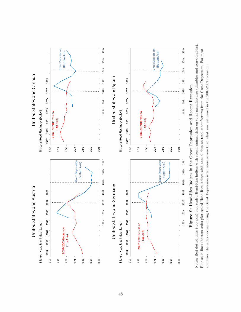
Figure9:Head-RiesIndicesintheGreatDepressionandRecentRecession

Notes:Reddottedlines(topaxis)plotscaledHead-Riesindiceswithrecentannualdataontotalmanufactures(durablesandnon-durables).

Bluesolidlines(bottomaxis)plotscaledHead-Riesindiceswithannualdataontotalmanufacturesfrom

theGreatDepression.Formost

countries,theindexdeclineduringtheGreatDepressionisfarmoreseverethanwhatwaswitnessedinthe2007-2009recession.

48

Figure10:Head-RiesIndicesintheGreatDepressionandRecentRecession

Notes:Reddottedlines(topaxis)plotscaledHead-Riesindiceswithrecentannualdataontotalmanufactures(durablesandnon-durables).

Bluesolidlines(bottomaxis)plotscaledHead-Riesindiceswithannualdataontotalmanufacturesfrom

theGreatDepression.Formost

countries,theindexdeclineduringtheGreatDepressionisfarmoreseverethanwhatwaswitnessedinthe2007-2009recession.

49

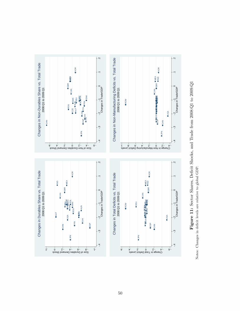
AU

T

CA

NC

HN

CZE

DN

K

FIN

FRAD

EU GR

C

HU

N

IND

ITA

JPN

MEX

POL

RO

U

SVK

KOR

ESP

SWE

GBR

US

AR

OW

1.8.6.4.20.2Size of Durables Demand Shock

.4.3

.2.1

0.1

.2C

hang

es in

Tra

de/G

DP

2008

:Q1

to 2

009:

Q1

Cha

nges

in D

urab

les

Shar

e vs

. Tot

al T

rade

AU

T

CA

N

CH

N

CZE

DN

KFI

NFR

ADE

U GR

C

HU

N

IND

ITA

JPN

MEX

POL

RO

U

SVK

KOR

ESP

SWE

GBR

US

AR

OW

.6.4.20.2.4.6Size of NonDurables Demand Shock

.4.3

.2.1

0.1

.2C

hang

es in

Tra

de/G

DP

2008

:Q1

to 2

009:

Q1

Cha

nges

in N

onD

urab

les

Shar

e vs

. Tot

al T

rade

AU

TC

AN

CH

N

CZE

DN

KFI

NFR

ADE

U GR

CH

UN

IND

ITA

JPN

MEX

POL

RO

USV

K

KOR

ESP

SWE

GBR

US

A

RO

W

.6.4.20.2.4.6Change in Total Deficit Levels

.4.3

.2.1

0.1

.2C

hang

es in

Tra

de/G

DP

2008

:Q1

to 2

009:

Q1

Cha

nges

in T

otal

Def

icits

vs.

Tot

al T

rade

AU

TC

AN

CH

N

CZE

DN

KFI

NFR

A DE

UGR

CH

UN

IND

ITA

JPN

MEX

POL

RO

USV

KKO

RES

PSW

EG

BR

US

A

RO

W

.4.20.2.4.6.81Change in NonManufacturing Deficit Levels

.4.3

.2.1

0.1

.2C

hang

es in

Tra

de/G

DP

2008

:Q1

to 2

009:

Q1

Cha

nges

in N

onM

anuf

actu

ring

Def

icits

vs.

Tot

al T

rade

Figure11:SectorShares,De�citShocks,andTradefrom

2008:Q1to2009:Q1

Notes:Changesinde�citlevelsarerelativetoglobalGDP.

50

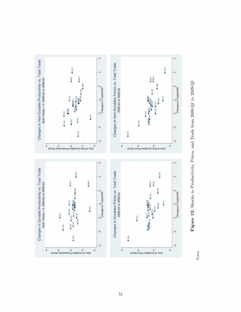
AU

T

CA

N

CH

N

CZE

DN

KFI

NFR

A DE

UGR

C

HU

N

IND

ITA

JPN

MEX

POL

RO

U

SVK

KOR

ESP

SWE

GBR

US

AR

OW

.4.20.2.4Size of Durables Productivity Shock

.4.3

.2.1

0.1

.2C

hang

es in

Tra

de/G

DP

Both

The

tas

= 2;

200

8:Q

1 to

200

9:Q

1C

hang

es in

Dur

able

Pro

duct

ivity

vs.

Tot

al T

rade

AU

T

CA

N

CH

N

CZE

DN

KFI

N

FRA D

EUGR

CH

UN

IND

ITA

JPN

MEX

POL

RO

U

SVK

KOR

ESP

SWE

GBR

US

A

RO

W

.2.10.1.2Size of NonDurables Productivity Shock

.4.3

.2.1

0.1

.2C

hang

es in

Tra

de/G

DP

Both

The

tas

= 2;

200

8:Q

1 to

200

9:Q

1C

hang

es in

Non

Dur

able

Pro

duct

ivity

vs.

Tot

al T

rade

AU

T

CA

NC

HN

CZE

DN

KFI

NFR

A DE

U GR

C

HU

NIN

D

ITA

JPN

MEX

POL

RO

USV

K

KOR

ESP

SWE

GBR

US

A

RO

W

.4.20.2Size of Durables Price Shock

.4.3

.2.1

0.1

.2C

hang

es in

Tra

de/G

DP

2008

:Q1

to 2

009:

Q1

Cha

nges

in D

urab

les

Pric

es v

s. T

otal

Tra

de

AU

T

CA

N

CH

N

CZE

DN

KFI

N

FRAD

EUGR

C

HU

N

IND

ITA

JPN

MEX

POL

RO

USV

K

KOR

ESP

SWE

GBR

US

A

RO

W

.4.20.2Size of NonDurables Price Shock

.4.3

.2.1

0.1

.2C

hang

es in

Tra

de/G

DP

2008

:Q1

to 2

009:

Q1

Cha

nges

in N

onD

urab

les

Pric

es v

s. T

otal

Tra

de

Figure12:ShockstoProductivity,Prices,andTradefrom

2008:Q1to2009:Q1

Notes:

51

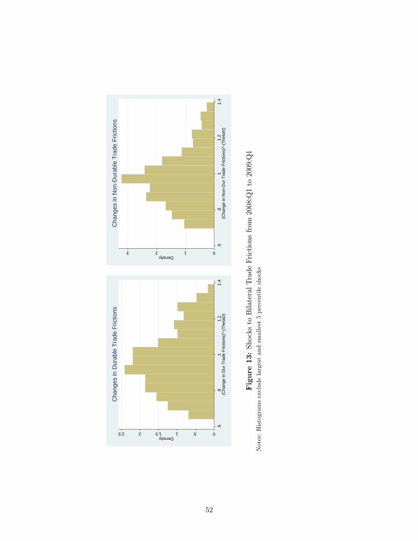
0.511.522.5Density

.6.8

11.

21.

4(C

hang

e in

Dur

Tra

de F

rictio

ns)^

(The

taD

)

Cha

nges

in D

urab

le T

rade

Fric

tions

0123Density

.6.8

11.

21.

4(C

hang

e in

Non

Dur

Tra

de F

rictio

ns)^

(Th

etaN

)

Cha

nges

in N

onD

urab

le T

rade

Fric

tions

Figure13:ShockstoBilateralTradeFrictionsfrom

2008:Q1to2009:Q1

Notes:Histogramsexcludelargestandsmallest5percentileshocks

52

Figure14:GlobalTrade/GDPAcrossManyFour-QuarterPeriodsinDataandCounterfactuals

Notes:

53

Figure15:CountryTrade/GDPAcrossManyFour-QuarterPeriodsinDataandCounterfactuals

Notes:�D=�N

=2

54

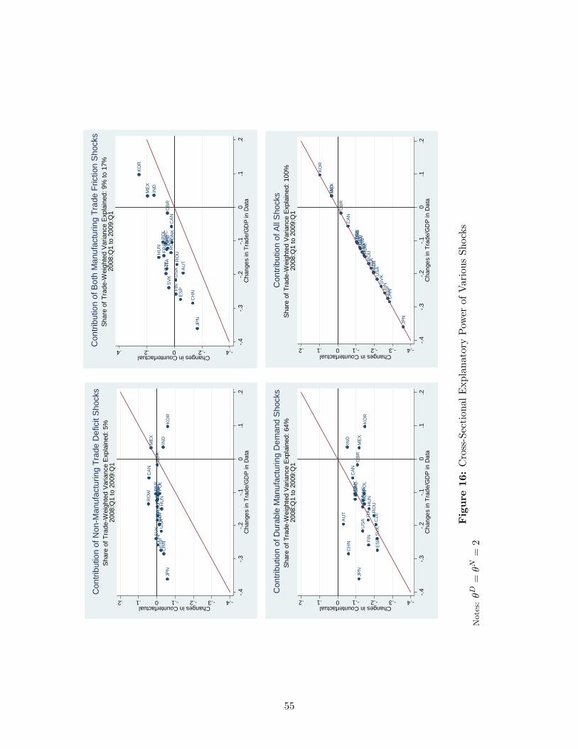
AU

T

CA

N

CH

NC

ZED

NK

FIN

FRA D

EU GR

CH

UN

IND

ITA

JPN

MEX

POL

RO

USV

K

KOR

ESP

SWE

GBR

US

A

RO

W.4.3.2.10.1.2

Changes in Counterfactual

.4.3

.2.1

0.1

.2C

hang

es in

Tra

de/G

DP

in D

ata

Shar

e of

Tra

deW

eigh

ted

Varia

nce

Exp

lain

ed: 5

%20

08:Q

1 to

200

9:Q

1

Con

tribu

tion

of N

onM

anuf

actu

ring

Trad

e D

efic

it Sh

ocks

AU

T

CA

N

CH

N

CZE

DN

KFI

N

FRA D

EUGR

CH

UN

IND

ITA

JPN

MEX

POL

RO

U

SVK

KOR

ESP

SWE

GBR

US

AR

OW

.4.20.2.4Changes in Counterfactual

.4.3

.2.1

0.1

.2C

hang

es in

Tra

de/G

DP

in D

ata

Shar

e of

Tra

deW

eigh

ted

Varia

nce

Exp

lain

ed: 9

% to

17%

2008

:Q1

to 2

009:

Q1

Con

tribu

tion

of B

oth

Man

ufac

turin

g Tr

ade

Fric

tion

Sho

cks

AU

T

CA

NC

HN

CZE

DN

K

FIN

FRAD

EU GR

C

HU

N

IND

ITA

JPN

MEX

POL

RO

USV

K

KOR

ESP

SWE

GBR

US

AR

OW

.4.3.2.10.1.2Changes in Counterfactual

.4.3

.2.1

0.1

.2C

hang

es in

Tra

de/G

DP

in D

ata

Shar

e of

Tra

deW

eigh

ted

Varia

nce

Exp

lain

ed: 6

4%20

08:Q

1 to

200

9:Q

1

Con

tribu

tion

of D

urab

le M

anuf

actu

ring

Dem

and

Sho

cks

AU

T

CA

N

CH

N

CZE

DN

K

FIN

FRAD

EUGR

CH

UN

IND

ITA

JPN

MEX

POL

RO

U

SVK

KOR

ESP

SWE

GBR

US

A

RO

W

.4.3.2.10.1.2Changes in Counterfactual

.4.3

.2.1

0.1

.2C

hang

es in

Tra

de/G

DP

in D

ata

Shar

e of

Tra

deW

eigh

ted

Varia

nce

Exp

lain

ed: 1

00%

2008

:Q1

to 2

009:

Q1

Con

tribu

tion

of A

ll S

hock

s

Figure16:Cross-SectionalExplanatoryPowerofVariousShocks

Notes:�D=�N

=2

55

FigureB1:CheckingAccuracyofTemporalDisaggregationProcedureforU.S.

Notes:Checkingprocedurewithdurable(AMDMVS)andnon-durable(AMNMVS)seriesfrom

FederalReserve

M3survey(notethisisdi¤erentsourcefrom

analysisinpaper).Annualtotalsincludedfrom

1995-2007only,

eventhoughdatastartsearlierandisavailablethrough2009,tomirrorextentofdatausedforothercountries.

56

Appendix A: Derivations of Expression (11)In this appendix, we demonstrate that one can derive the Head-Ries index from many classes of trade models,such as a structure with Armington preferences, as in Anderson and van Wincoop (2003), monopolisticcompetition as in Redding and Venables (2004), the Ricardian structure in Eaton and Kortum (2002), ormonopolistic competition with heterogeneous producers, as in Melitz (2003) and Chaney (2008). To do so,we need only show that each theory of international trade lead to a bilateral import share equation with thesame form as equation (11). From there, the derivation of (15) follows exactly as in Section 2. This impliesthat for the �rst sections of the paper, we need not specify a particular trade structure, so long as it is inthis larger set of models.

1. Consider the model of Armington (1969), as implemented in Anderson and van Wincoop (2003).Consumers in country n maximize: X

i

�(1��)=�i c

(��1)=�ni

!�=(��1);

subject to the budget constraintP

i pnicni = yn, where � is a preference parameter representing theelasticity of substitution across goods produced in di¤erent countries, �i > 0 is a parameter capturingthe desirability of of country i�s goods, yn is the nominal income of country n, and pni and cni arethe price and quantity of the traded good supplied by country i to country n. In their setup, pricesre�ect a producer-speci�c cost and a bilateral-speci�c trade cost: pni = pitni. Solving for the nominaldemand of country i for goods from country j then yields their equation (6):

xni =

��ipitniPn

�1��yn;

where Pn =hP

k (�kpktnk)1��i1=(1��)

is the price index of country n. Substituting this de�nition

and with goods markets clearing, yn =P

j xnj , we obtain:

�ni =xniPj xnj

=(�ipitni)

1��Pk (�kpktnk)

1�� .

Relabeling � = � � 1 and Ti = ��i , we recover an expression equivalent to (11).

2. Consider the model of Krugman (1980), as implemented in Redding and Venables (2004). Like An-derson and van Wincoop, they use a constant elasticity formulation, but they include a �xed cost for�rms operating in each country. They express, in their equation (9), the total value of imports tocountry n from i:

xni =�nip

1��i

�t1��ni

�EnG

��1n

�;

where they refer to�EnG

��1n

�as the "market capacity" of the importing country n because it refers

to the size of n�s market, the number of competing �rms that can cover the �xed cost of operation,and the level of competition as summarized by the price index G. They refer to the term

�nip

1��i

�as

the "supply capacity" of the exporting country i, because �xing the market capacity, the volume ofsales is linearly homogeneous in that term. Finally, T 1��ni is the iceberg trade cost for shipping from ito n. Hence, this model too leads to an expression:

�ni =xniPj xnj

=

�nip

1��i

�T 1��niP

k

�nkp

1��k

�T 1��nk

.

Again, this expression can be relabeled and made equivalent to (11).

3. Consider the competitive model of Eaton and Kortum (2002), where � and Ti are parameters ofa Fréchet distribution of producer e¢ ciency capturing, respectively, heterogeneity across producers(inversely) and country i�s absolute advantage. The property of this distribution is such that theprobability that country i is the lowest price (production plus transport costs) provider of a good to

57

country n is an expression identical to (11), their equation (8). Given that average expenditure pergood in their model does not vary by source and invoking the low of large numbers, it follows thatthis probability is equivalent to the trade share.

4. Consider Chaney (2008), which builds on Melitz (2003). Firm productivities are distributed Paretowith shape parameter and in addition to iceberg costs �ni, to sell in market n also requires employingfni units of local labor. This leads to an expression for total imports by country n from country i, hisequation (10) (where we�ve dropped sectoral terms indexed by h):

xni =YiYnY

� nw� i �� ni f

�[ =(��1)�1]ni ;

where notation is similar to the examples above, and �n measures what he refers to as country n�s"remoteness" from the rest of the world. Summing this over all bilaterals implies:

�ni =xniPj xnj

=Yiw

� i

��nif

[1=(��1)�1= ]ni

�� P

k Ykw� k

��nkf

[1=(��1)�1= ]nk

�� ;which, again, is clearly in the same form as (11).

58

Appendix B: Data Sources and Related ProceduresIn this appendix, we �rst detail our sources for trade, production, input-output, and macroeconomic data.We next describe the construction of sectoral industrial production and producer price indices and reviewthe temporal disaggregation procedure that uses these indices along with annual data to generate monthlyproduction values for each manufacturing sector. Finally, we list the data sources and procedures requiredto calculate the Head-Ries index on Great Depression-era data.

Trade DataTrade data are readily available at a monthly frequency �we use monthly bilateral trade data from theGlobal Trade Atlas Database. These data are not seasonally adjusted and are provided in dollars. Weaggregate appropriate 2-digit HS categories to generate the total bilateral and multilateral trade �ows ineach manufacturing sector.

Concordances Linking Trade and ProductionA many-to-many concordance was constructed to link the 2-digit harmonized system (HS) trade data tothe International Standard Industrial Classi�cation (ISIC) codes used in the production data. We start bydownloading the mapping of 6-digit HS codes (including all revisions) to ISIC codes from the WITS website.This concordance was then merged with COMTRADE data on the volume of world trade at the 6-digitlevel for 2007-2008 (also accessed through WITS). We estimate the proportion of each HS 2-digit code thatbelongs in each ISIC category using these detailed worldwide trade weights. Then we can use the sameconcordance in the last step to map production and trade to our sectors j 2 M .

Input-Output Coe¢ cients

The input-output coe¢ cients ��ji and jli �were calculated from the 2009 edition of the OECD�s country

tables.22 We concord and combine the 48 sectors used in these tables to form input-output tables for thethree sectors j 2 . Table B1 shows how we classi�ed these 48 sectors into durables, non-durables, andnon-manufactures. To determine �ji , we divide the total value added in sector j of country i by that sector�stotal output. To determine the values for jli , we divide total spending in country i by sector j on inputsfrom sector l and divide this by that sector�s total intermediate use at basic prices (i.e. net of taxes onproducts). The OECD input-output tables are often available for the same countries for multiple years. Insuch cases, we use the most recent year of data available.

Additional Macro DataExchange rates to translate local currency production values into dollars (to match the dollar-denominatedtrade �ows) are from the OECD.Stat database and from the International Financial Statistics database fromthe IMF. Other standard data used in the paper, such as quarterly GDP and trade de�cits, are taken fromthe Economist Intelligence Unit (EUI). Trade and production data are translated using exchange rates atthe monthly frequency before being aggregated to the quarterly frequency that we use in our regressions andcounterfactuals.

IP and PPI Indices by SectorTo generate monthly production levels for durables and non-durables, we �rst need IP and PPI indices atthe sector level. The exact methodology used to construct the series depended on what series were availableon DataStream, as this is not consistent across countries. Essentially, three di¤erent methodologies wereused.

We applied a �rst methodology when Datastream contains IP or PPI series on durable manufacturingand nondurable manufacturing for the country. Included in this category for IP are Canada, China, andthe United States. Included in this category for PPI are China and the United States. For China the seriesare actually "Heavy Industry" and "Light Industry". The key di¤erence appears to be that one group ofnondurable manufactures - chemicals - is included in heavy industry.

22The only exception is China�s input-output table, which was obtained from Robert Feenstra and is analyzed inFeenstra and Hong (2007).

59

Next, there are several countries for which Datastream contains IP or PPI series for capital goods,durable consumer goods, nondurable consumer goods, and intermediate goods. We classify capital goods asdurable, but need to be able to decompose the intermediate goods into durable goods (such as metals) andnondurable goods (such as paper). The presence of more detailed manufacturing industry data allows us todo this using regression analysis. We regress monthly log-changes in intermediate goods IP or PPI series onunderlying detailed manufacturing industry series to reveal the composition of the intermediate series andexclude countries for which there is not a good �t. The regression results give us estimates of the industrycomposition of intermediate goods manufacturing, and we combine this with our industry concordances todurable and non-durable to generate durable and nondurable intermediate goods IP or PPI series. We thencombine all the more aggregated categories, using their weights in production from the annual data, togenerate indices for overall durables and non-durables. This methodology applies to the construction of ourIP and PPI series for Austria, Czech Republic, Denmark, Finland, France, Germany, Greece, Hungary, Italy,Romania, Slovakia, South Korea, Spain, Sweden, and the United Kingdom.

There are some countries with IP or PPI data for multiple manufacturing industries together withaggregate manufacturing (or occasionally, total industry IP or PPI).We use similar regression analysis toascertain the industry composition of the broad measure, and then use our data on the durable and non-durable composition of each of these industries to construct durable and nondurable series. When theregression analysis does not yield a good �t (judged by a high R-squared and coe¢ cients that sum close to1), we do not include that country. This procedure was used for India, Japan, Mexico and Poland.

Finally, we also require IP and PPI indices for overall manufacturing. These monthly data for China werefound at chinadataonline.com, and for the other countries were downloaded from the OECD Main EconomicIndicators Database (MEI) and the EIU Database.

Annual Production by SectorIn addition to monthly IP and PPI indices, we need annual production levels for each sector and for overallmanufacturing. These annual data are taken from the OECD Structural Analysis Database (STAN) and theUnited Nations National Accounts and Industrial Statistics Database (UNIDO). For China, Chang-Tai Hsiehprovided us with cross-tabs from 4-digit manufacturing production data from the census of manufacturingproduction. We used these data to determine the durables/non-durables split and multipled these shares bythe manufacturing total from http://chinadataonline.org.

We concord International Standard Industrial Classi�cation (ISIC Rev. 3) 2-digit manufacturing pro-duction data to the appropriate sector de�nition (whatever is required to match the IP/PPI indices) toget annual totals for each of these categories.23 Our de�nition of manufacturing comprises ISIC industries15 through 36 excluding 23 (petroleum). We further divide goods into capital goods, durable consumergoods, nondurable consumer goods, durable intermediate goods, and non-durable intermediate goods usingthe U.S. import end use classi�cation. Harmonized System (HS) trade data are simultaneously mapped intothe end use classi�cation using a concordance from the U.S. Census Bureau and into the ISIC classi�cationusing the concordances from the World Bank�s World Integrated Trade Solution (WITS) website. Worldtrade volumes at the 6-digit level for 2007-2008 are again used to estimate what proportion of each ISICclassi�cation belongs in each of the categories.

Temporal DisaggregationThe United States reports monthly estimates of the level of manufacturing production, but such data arenot available for most of the countries we study. However, annual production data in levels are availablefor all of these countries. We now describe how we use the monthly indicators of production constructed asdescribed above to disaggregate annual production levels into internally consistent monthly values, as wellas to generate out-of-sample predictions that re�ect all up-to-date information for the months subsequent tothe previous year�s end. This problem, referred to in the econometrics and forecasting literature as temporaldisaggregation, was studied as early as the 1950s by, among others, Milton Friedman (see Friedman, 1962).

We disaggregate and extrapolating the annual production data in country i and sector j using theestimated relationship with the industrial production and producer price indices in that same country andsector.24 The details follow below, but for intuition, think of a linear regression of the annual gross productionof manufacturers on the annual sum of the monthly totals of the high frequency variables. Chow and Lin(1971) starts by using the coe¢ cient estimates from such a regression to generate predicted monthly values.

23Occasionally, a 2-digit sector will be dropped for one year, so we impute an alternative series where productionlevels are "grown" backward from the more recent and most complete data, only using the growth rates from categoriesreported in both years.24The procedure was adapted from the code in Quilis, Enrique. �A Matlab Library of Temporal Disaggregation

and Interpolation Methods: Summary,�2006.

60

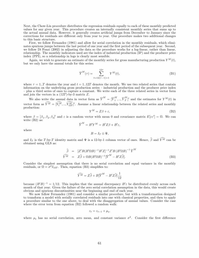
Next, the Chow-Lin procedure distributes the regression residuals equally to each of these monthly predictedvalues for any given year. This procedure creates an internally consistent monthly series that sums up tothe actual annual data. However, it generally creates arti�cial jumps from December to January since thecorrections for residuals are di¤erent only from year to year. Our procedure makes two additional changesto this basic structure.

First, we follow Fernandez (1981) and allow for serial correlation in the monthly residuals, which elimi-nates spurious jumps between the last period of one year and the �rst period of the subsequent year. Second,we follow Di Fonzi (2002) in adjusting the data so the procedure works for a log-linear, rather than linear,relationship. The monthly indicators used are the index of industrial production (IP) and the producer priceindex (PPI), so a relationship in logs is clearly most sensible.

Again, we wish to generate an estimate of the monthly series for gross manufacturing production YM (t),but we only have the annual totals for this series:

YM(�) =

12�Xt=12(��1)+1

YM (t); (B1)

where � = 1::T denotes the year and t = 1::12T denotes the month. We use two related series that containinformation on the underlying gross production series �industrial production and the producer price index�plus a third series of ones to capture a constant. We write each of the three related series in vector formand join the vectors in a (12T )-by-3 matrix Z.

We also write the annual data in vector form as YM= [Y

M

1 ; ::; YM

T ]0 and the estimates for YM (t) in

vector form as dYM = [dYM1 ; ::;[YM12T ]0. Assume a linear relationship between the related series and monthlyproduction:

YM = Z� + "; (B2)

where � = [�1; �2; �3]0 and " is a random vector with mean 0 and covariance matrix E[""0] = . We can

write (B2) as:

YM= B0YM = B0Z� +B0";

whereB = IT ;

and IT is the T -by-T identity matrix and is a 12-by-1 column vector of ones. Hence, b� and dYM can beobtained using GLS as:

b� = [Z 0B(B0B)�1B0Z]�1Z 0B (B0B)�1YM

dYM = Zb� +B(B0B)�1[YM �B0Zb�]: (B3)

Consider the simplest assumption that there is no serial correlation and equal variance in the monthlyresiduals, or = �2I12T . Then, equation (B3) simpli�es to:

dYM = Zb� +B[YM �B0Zb�] 112

because (B0B)�1 = 1=12. This implies that the annual discrepancy B0" be distributed evenly across eachmonth of that year. Given the failure of the zero serial correlation assumption in the data, this would createobvious and spurious discontinuities near the beginning and end of each year.

We now follow Fernandez (1981) and consider a similar procedure, but with a transformation designedto transform a model with serially correlated residuals into one with classical properties, and then to applya procedure similar to the one above, to deal with the disaggregation of annual values. Consider the casewhere the error term from equation (B2) followed a random walk:

"t = "t�1 + �t;

where �t has no serial correlation, zero mean, and constant variance �2. Consider the �rst di¤erence

61

transformation D:

D12T -by-12T =

2666641 0 0 : 0 0�1 1 0 : 0 00 �1 1 : 0 0: : : : : :: : : : : :0 0 0 : �1 1

377775 :One can premultiply the error in equation (B2) by this matrix to generate: DYM�DZ�, which converts

the both left and right hand sides of the model into �rst-di¤erence form, with the exception being the �rstterms given the upper left hand element equals one. With these �rst-di¤erenced series, we can re-write themodel as:

DYM= DZ� +D":

Note that = E[D""0D0] = E[��0] = �2I12T , so errors in this reformulated model have classical properties.Fernandez shows that the expression for the best linear estimator in this context is the same as (B3), butwith = (D0D)

�1:

b� = [Z 0B(B0 (D0D)�1B)�1B0Z]�1Z 0B

�B0 (D0D)

�1B��1

YM

dYM = Zb� + (D0D)�1B(B0 (D0D)

�1B)�1[Y

M �B0Zb�]: (B4)

The relationship (B2) is written in levels, but it is clearly more appropriate for our purposes to writethe relationship between production and production indicators in log-levels, such that a given percentagechange in one variable leads to a percentage change in the other:

lnYM = (lnZ)� + ": (B5)

This can be somewhat di¢ cult to handle in the above framework because the sum of the log of monthly totalswill not equal the log of the annual total when the adding-up constrain does hold in levels. We deal with thisby running the algorithm on annual data that has been converted such that the sum of �tted monthly datawill approximate the original annual levels. This cannot be achieved exactly, so a second-stage procedure isthen implemented to distribute the residuals across the months and ensure the aggregation constraints bindexactly.

Following Di Fonzi (2002), we consider the �rst order Taylor series approximation of lnYM around the

log of the arithmetic average for the monthly totals, ln(YM=12). We write:

lnYM = gYM � ln YM

12+12

YM

YM � Y

M

12

!= lnY

M � ln 12 + 12YM

YM� 1.

Summing this expression up over the twelve months, we get:

12Xj=1

gYMj = 12 lnYM � 12 ln 12.

Hence, we can follow the above procedure, except we replace the left hand size of (B5) withgYM = 12 lnYM�

12 ln 12 and the right hand size withP12

j=1 lnZj .This approximation should come close to satisfying the temporal aggregation constraints, but will fail to

do so exactly. Hence, the �nal step is to adjust the estimates following Denton (1971). Denoting the initial

�tted values as dYM and the residuals YM �

12Xt=1

dYMt = R (in vector form), we make the �nal adjustment:

[YM� = dYM + (D0D)�1B0(B (D0D)

�1B0)�1R:

To check the quality of the procedure, we compared the monthly �tted series produced using this algo-rithm and the actual monthly data released by the U.S. Census Bureau on the value of shipments in durableand non-durable manufacturing. The U.S. monthly data are collected as part of the M3 manufacturing

62

survey.25 In all other parts of the paper, our monthly series sum to the annual production totals found inthe UN and OECD data, but for this test of the algorithm we re-run the procedure using annual totals fromthe M3 survey. Though M3 data are available through 2009, we only use annual totals for 1995-2007 toensure the procedure uses the same amount of data as we would have for other countries in our sample. Wetest both a procedure which estimates the beta coe¢ cients from (B2) for the relationship between annualproduction and the monthly indicators as well as one in which we set the coe¢ cients in the relationshipequal to one for all countries and sectors.

Appendix Figure B1 demonstrates that both procedures do an excellent job of matching movementsin the time series for non-durables, including the out-of-sample decline in production during the recentrecession. Our "Beta equals 1" procedure does an excellent job both in-sample and out-of sample. Theprocedure with estimated coe¢ cients underestimates the decline in production of durables during the recentrecession. Given this, the results in the text re�ect the results of this procedure when the beta coe¢ cientsfrom (B2) for the relationship between production and IP/PPI are automatically set equal to one, implyingthat the product of IP and PPI will generally move perfectly with nominal production. We have checked allour results with the endogenous estimation of these beta coe¢ cients and none of the global results changesmeaningfully.

When applied at the sector level, this procedure generates monthly series of these disaggregated categoriesfrom which we obtain a monthly series of the share of durables in manufacturing. Given the highest qualityproduction data from these databases are for the total manufacturing sector, we then multiply these sharesby total manufacturing production, which is interpolated in exactly the same way but with IP/PPI indicesfor the whole of manufacturing. We then have monthly series for durable and non-durable manufacturingproduction which are consistent with published annual (and implied monthly) levels of total manufacturingproduction.

Calculating Head-Ries Indices During the Great DepressionWe obtained data on bilateral and multilateral manufacturing trade as well as exchange rates for 1926-1937from the annual Foreign Commerce Yearbooks, published by the U.S. Department of Commerce. Total U.S.multilateral manufacturing imports and exports were taken from Carter et al. (2006). The gross valueof manufacturing, required for the denominator of (15), were obtained from a variety of country-speci�csources.26 The U.S. ratio of gross output to value added in manufacturing, found in Carter (2006), wasapplied to foreign manufacturing value added when output data were unavailable.

The bilateral trade and the manufacturing totals often re�ect changing availability of data for disaggre-gated categories. For example, one year�s total growth may re�ect both 20% growth in Paper Products aswell as the initial measurement (relative to previous missing values) of Transportation Equipment. Sinceinspection suggests that such missing values do not simply re�ect zero values, we calculate year-to-yeargrowth rates using only the common set of recorded goods. For manufacturing production, we not only needthe growth rate, but the level also matters because we subtract the level of exports to measure absorption.We apply the growth rate backwards from the most complete, typically also the most recent, series value.

25The monthly totals are extrapolated from a sampling procedure that covers a majority of manufacturerswith $500 million or more in annual shipments as well as selected smaller companies in certain industries. Seehttp://www.census.gov/indicator/www/m3/m3desc.pdf for additional details.26Where needed, U.S. Department of Commerce (1968) was used to translate currency or physical units into U.S.

dollars. Austria: Bundesamt fur Statistik (1927-1936) was used to obtain product-speci�c production data, either inhundreds of Austrian schilling or in kilograms. Canada: Value of manufacturing data were available in U.S. dollarsfrom Urquhart (1983). Germany: Data were obtained from Statistishen Reichsamt (1931, 1935, 1940). Finland,Japan, Spain, and Sweden: Value added in manufacturing, in local currency units, were taken from Smits (2009).Peru: Output data in Peruvian pounds and soles obtained from Ministerio de Hacienda y Comercio (1939). UnitedKingdom: Data were obtained from United Kingdom Board of Trade (1938). These annual numbers combined lessfrequent results from the censuses in 1924, 1930, and 1935, with industrial production data, taken yearly, from1927-1937.

63

Appendix C: Trade Frictions and ProductivityIn this appendix, we describe how changes in trade frictions and changes in productivity are intimatelyconnected. We can bring out this connection, and get some insights into the logic of the model, by combiningtrade friction shocks and productivity shocks in the term:

�j

ni =�jn

�jidjni; (C1)

where the �ji represent productivity changes through:

Aji =��ji

�1�e jji (1�e�ji ) ��li

��e jli (1�e�ji ): (C2)

In addition, we de�ne a productivity-adjusted price change by

qji = pji �

ji : (C3)

Using this reparameterization, (17) and (18) remain unchanged while (19) becomes:

qjn =

IXi=1


�qji

��je jji (1�e�ji ) �qli��je jli (1�e�ji ) ��jni��j

!�1=�j; (C4)

and (20) becomes:

��jni

�0= �jniw

��je�jii

�qji

��je jji (1�e�ji ) �qli��je jli (1�e�ji ) �jni

qjn

!��j: (C5)

Note that productivity changes do not enter directly into (C4) or (C5) as they are embedded in the �j

ni andqji .

The solution to (17), (18), (C4), and (C5) is also the solution to (17), (18), (19), and (20). To see why,substitute (C1) into (C4) to get:

qjn =

0@ IXi=1


�qji

��je jji (1�e�ji ) �qli��je jli (1�e�ji ) �jn

�jidjni

!��j1A�1=�j

:

Grouping terms, the left hand side becomes qjn=�jn and the price terms on the right hand side become

qji =�ji and q

li=�

li, leaving a term on the right hand side equal to

��ji

��j [1�e jji (1�e�ji )] ��li

��je jli (1�e�ji ). This

expression then replicates (19) after substituting in (C3) and (C2). Similarly, substituting (C1) into (C5),applying (C3) and (C2), yields (20).

One implication of this result is that productivity shocks of the form

Aji = �e�ji ;

for any � > 0, leave equilibrium wages, spending, and trade shares una¤ected. The resulting price changesare pji = 1=� for j 2 M . Furthermore, changes in service-sector productivity do not change equilibriumoutcomes given the Aji . Such changes would have welfare consequences, but are irrelevant to the equilibriumconsidered here.

Another implication of this result is that to solve the model for changes in wages and trade shares, all

we need is �j

ni rather than djni and A

ji separately. We can decompose the contribution of trade friction and

productivity shocks using additional restrictions or data, as we do above with data on sectoral price changes.

If we do not wish to impose further restrictions, we can calibrateion the �j

ni directly. Start by dividing

64

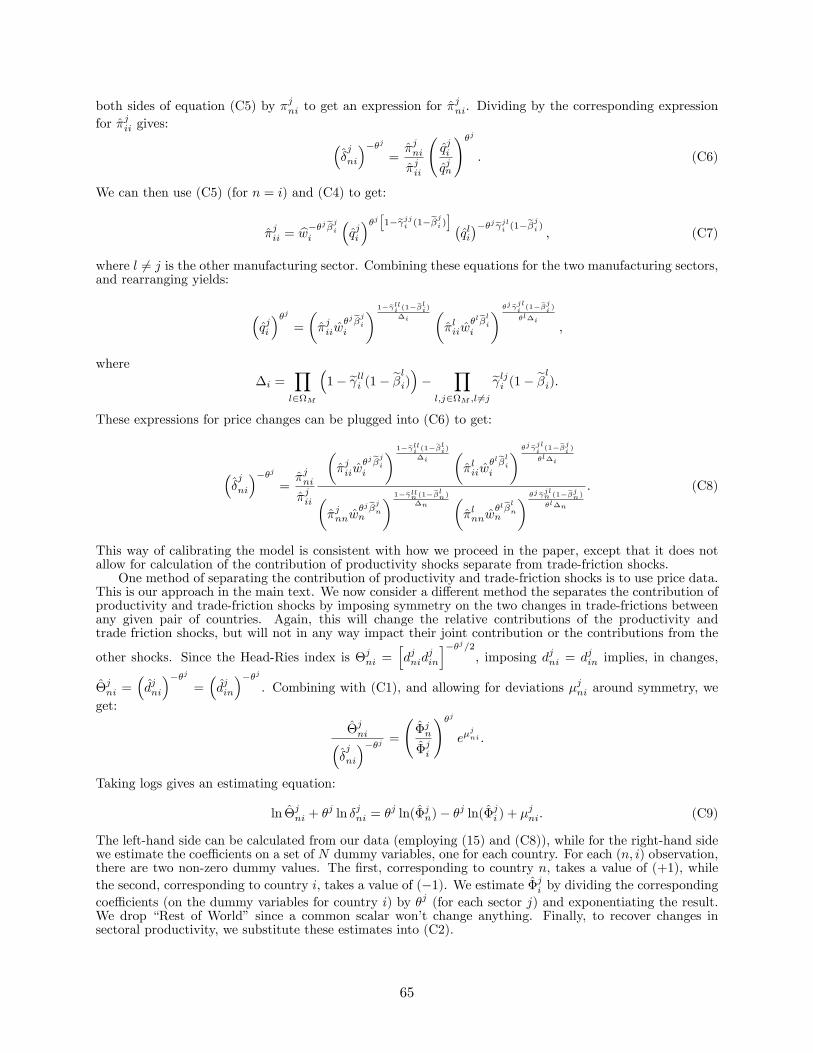
both sides of equation (C5) by �jni to get an expression for �jni. Dividing by the corresponding expression

for �jii gives: ��j

ni


qjiqjn

!�j: (C6)

We can then use (C5) (for n = i) and (C4) to get:

�jii = bw��je�jii

�qji

��jh1�e jji (1�e�ji )i �qli��je jli (1�e�ji ) ; (C7)

where l 6= j is the other manufacturing sector. Combining these equations for the two manufacturing sectors,and rearranging yields:

�qji

��j=

��jiiw

�je�jii

� 1�e lli (1�e�li)�i

��liiw

�le�lii

� �j e jli(1�e�j

i)

�l�i

;

where�i =

Yl2M

�1� e lli (1� e�li)�� Y

l;j2M ;l 6=je lji (1� e�li):

These expressions for price changes can be plugged into (C6) to get:

��j

ni


��jiiw

�je�jii

� 1�e lli (1�e�li)�i

��liiw

�le�lii

� �j e jli(1�e�j

i)

�l�i

��jnnw

�je�jnn

� 1�e lln (1�e�ln)�n

��lnnw

�le�lnn

� �j e jln (1�e�jn)�l�n

: (C8)

This way of calibrating the model is consistent with how we proceed in the paper, except that it does notallow for calculation of the contribution of productivity shocks separate from trade-friction shocks.

One method of separating the contribution of productivity and trade-friction shocks is to use price data.This is our approach in the main text. We now consider a di¤erent method the separates the contribution ofproductivity and trade-friction shocks by imposing symmetry on the two changes in trade-frictions betweenany given pair of countries. Again, this will change the relative contributions of the productivity andtrade friction shocks, but will not in any way impact their joint contribution or the contributions from the

other shocks. Since the Head-Ries index is �jni =hdjnid

jin

i��j=2, imposing djni = djin implies, in changes,

�jni =�djni

��j=�djin

��j. Combining with (C1), and allowing for deviations �jni around symmetry, we

get:

�jni��j

ni

��j = �jn

�ji

!�je�

jni :

Taking logs gives an estimating equation:

ln �jni + �j ln �jni = �

j ln(�jn)� �j ln(�ji ) + �

jni: (C9)

The left-hand side can be calculated from our data (employing (15) and (C8)), while for the right-hand sidewe estimate the coe¢ cients on a set of N dummy variables, one for each country. For each (n; i) observation,there are two non-zero dummy values. The �rst, corresponding to country n, takes a value of (+1), whilethe second, corresponding to country i, takes a value of (�1). We estimate �ji by dividing the correspondingcoe¢ cients (on the dummy variables for country i) by �j (for each sector j) and exponentiating the result.We drop �Rest of World� since a common scalar won�t change anything. Finally, to recover changes insectoral productivity, we substitute these estimates into (C2).

65

Appendix D: Solving for the EquilibriumIn this appendix, we explain in more detail how we solve for the system�s equilibrium. Given a vector ofwage changes bw, we solve (19) and (20) jointly for changes in trade shares and prices. Denote the solutionfor changes in trade shares by �jni( bw) = ��jni�0.

Second, we can substitute the service sector out of equation (3) to get" �XDi

�0�XNi

�0 # = e�0i (Y 0i +D0i)� �i

�DSi

�0+ e�Ti

" �Y Di�0�

Y Ni�0 # ; (D1)

where the 2 by 1 vector e�i has elements�e�ji�0 = ��ji�0 + ��Si �0 �ji ;the 2 by 1 vector �i has elements

�ji = Sji (1� �

Si )

1� SSi (1� �Si );

and the 2 by 2 matrix e�i contains e jli (1� e�ji )in its j�th row and l�th column for all j; l 2 M .

Third, we follow the approach of Caliendo and Parro (2009) and substitute (21) into the right hand side

of (D1). Given wage changes, we obtain a linear system in the�Xji

�0�s by stacking (D1) across all countries:

X0 = (e�X)0 � ��DS�0 + e�T [�( bw)]T X0:Here

X0 =h�XD1

�0;�XD2

�0; :::;

�XDI

�0;�XN1

�0;�XN2

�0; :::;

�XNI

�0iT;

(e�X)0 = ��e�D1 X1�0 ;�e�D2 X2�0 ; :::;�e�DI XI�0 ;�e�N1 X1�0 ;�e�N2 X2�0 ; :::;�e�NI XI�0�T ;with �e�jiXi�0 = �e�ji�0 (wiYi +D0

i) ;��DS

�0=h�D1�DS1

�0; �D2

�DS2

�0; :::; �DI

�DSI

�0; �N1

�DS1

�0; �N2

�DS2

�0; :::; �NI

�DSI

�0iT;

e� =

266666666664

e DD1 (1� e�D1 ) 0 0 e DN1 (1� e�D1 ) 0 0

0. . . 0 0

. . . 0

0 0 e DDI (1� e�DI ) 0 0 e DNI (1� e�DI )e ND1 (1� e�N1 ) 0 0 e NN1 (1� e�N1 ) 0 0

0. . . 0 0

. . . 0

0 0 e NDI (1� e�NI ) 0 0 e NNI (1� e�NI )

377777777775;

and

�( bw) = � �D( bw) 00 �N ( bw)

�;

66

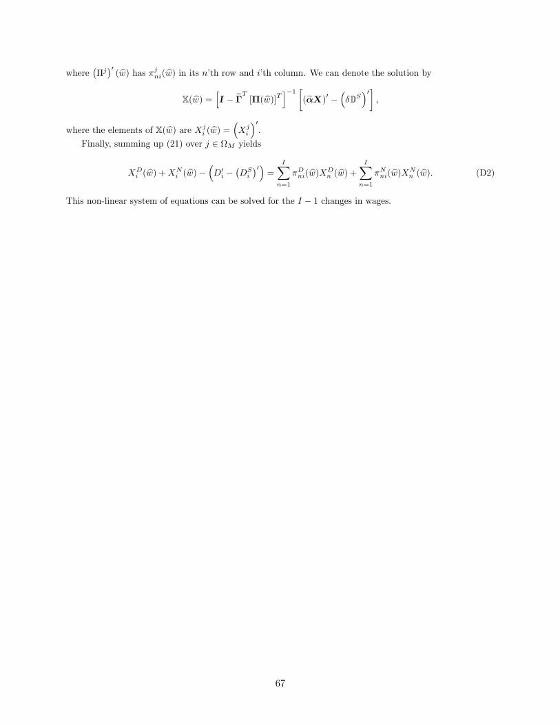
where��j�0( bw) has �jni( bw) in its n�th row and i�th column. We can denote the solution by

X( bw) = hI � e�T [�( bw)]T i�1 �(e�X)0 � ��DS�0� ;where the elements of X( bw) are Xj

i ( bw) = �Xji

�0.

Finally, summing up (21) over j 2 M yields

XDi ( bw) +XN

i ( bw)� �D0i ��DSi

�0�=

IXn=1

�Dni( bw)XDn ( bw) + IX

n=1

�Nni( bw)XNn ( bw): (D2)

This non-linear system of equations can be solved for the I � 1 changes in wages.

67

NBB WORKING PAPER No. 196 - OCTOBER 2010 69

NATIONAL BANK OF BELGIUM - WORKING PAPERS SERIES 1. "Model-based inflation forecasts and monetary policy rules", by M. Dombrecht and R. Wouters, Research

Series, February 2000. 2. "The use of robust estimators as measures of core inflation", by L. Aucremanne, Research Series,

February 2000. 3. "Performances économiques des Etats-Unis dans les années nonante", by A. Nyssens, P. Butzen and

P. Bisciari, Document Series, March 2000. 4. "A model with explicit expectations for Belgium", by P. Jeanfils, Research Series, March 2000. 5. "Growth in an open economy: Some recent developments", by S. Turnovsky, Research Series, May

2000. 6. "Knowledge, technology and economic growth: An OECD perspective", by I. Visco, A. Bassanini and

S. Scarpetta, Research Series, May 2000. 7. "Fiscal policy and growth in the context of European integration", by P. Masson, Research Series, May

2000. 8. "Economic growth and the labour market: Europe's challenge", by C. Wyplosz, Research Series, May

2000. 9. "The role of the exchange rate in economic growth: A euro-zone perspective", by R. MacDonald,

Research Series, May 2000. 10. "Monetary union and economic growth", by J. Vickers, Research Series, May 2000. 11. "Politique monétaire et prix des actifs: le cas des États-Unis", by Q. Wibaut, Document Series, August

2000. 12. "The Belgian industrial confidence indicator: Leading indicator of economic activity in the euro area?", by

J.-J. Vanhaelen, L. Dresse and J. De Mulder, Document Series, November 2000. 13. "Le financement des entreprises par capital-risque", by C. Rigo, Document Series, February 2001. 14. "La nouvelle économie" by P. Bisciari, Document Series, March 2001. 15. "De kostprijs van bankkredieten", by A. Bruggeman and R. Wouters, Document Series, April 2001. 16. "A guided tour of the world of rational expectations models and optimal policies", by Ph. Jeanfils,

Research Series, May 2001. 17. "Attractive prices and euro - Rounding effects on inflation", by L. Aucremanne and D. Cornille,

Documents Series, November 2001. 18. "The interest rate and credit channels in Belgium: An investigation with micro-level firm data", by

P. Butzen, C. Fuss and Ph. Vermeulen, Research series, December 2001. 19. "Openness, imperfect exchange rate pass-through and monetary policy", by F. Smets and R. Wouters,

Research series, March 2002. 20. "Inflation, relative prices and nominal rigidities", by L. Aucremanne, G. Brys, M. Hubert, P. J. Rousseeuw

and A. Struyf, Research series, April 2002. 21. "Lifting the burden: Fundamental tax reform and economic growth", by D. Jorgenson, Research series,

May 2002. 22. "What do we know about investment under uncertainty?", by L. Trigeorgis, Research series, May 2002. 23. "Investment, uncertainty and irreversibility: Evidence from Belgian accounting data" by D. Cassimon,

P.-J. Engelen, H. Meersman and M. Van Wouwe, Research series, May 2002. 24. "The impact of uncertainty on investment plans", by P. Butzen, C. Fuss and Ph. Vermeulen, Research

series, May 2002. 25. "Investment, protection, ownership, and the cost of capital", by Ch. P. Himmelberg, R. G. Hubbard and

I. Love, Research series, May 2002. 26. "Finance, uncertainty and investment: Assessing the gains and losses of a generalised non-linear

structural approach using Belgian panel data", by M. Gérard and F. Verschueren, Research series, May 2002.

27. "Capital structure, firm liquidity and growth", by R. Anderson, Research series, May 2002. 28. "Structural modelling of investment and financial constraints: Where do we stand?", by J.-B. Chatelain,

Research series, May 2002. 29. "Financing and investment interdependencies in unquoted Belgian companies: The role of venture

capital", by S. Manigart, K. Baeyens, I. Verschueren, Research series, May 2002. 30. "Development path and capital structure of Belgian biotechnology firms", by V. Bastin, A. Corhay,

G. Hübner and P.-A. Michel, Research series, May 2002. 31. "Governance as a source of managerial discipline", by J. Franks, Research series, May 2002. 32. "Financing constraints, fixed capital and R&D investment decisions of Belgian firms", by M. Cincera,

Research series, May 2002.


33. "Investment, R&D and liquidity constraints: A corporate governance approach to the Belgian evidence", by P. Van Cayseele, Research series, May 2002.

34. "On the origins of the Franco-German EMU controversies", by I. Maes, Research series, July 2002. 35. "An estimated dynamic stochastic general equilibrium model of the euro area", by F. Smets and

R. Wouters, Research series, October 2002. 36. "The labour market and fiscal impact of labour tax reductions: The case of reduction of employers' social

security contributions under a wage norm regime with automatic price indexing of wages", by K. Burggraeve and Ph. Du Caju, Research series, March 2003.

37. "Scope of asymmetries in the euro area", by S. Ide and Ph. Moës, Document series, March 2003. 38. "De autonijverheid in België: Het belang van het toeleveringsnetwerk rond de assemblage van

personenauto's", by F. Coppens and G. van Gastel, Document series, June 2003. 39. "La consommation privée en Belgique", by B. Eugène, Ph. Jeanfils and B. Robert, Document series,

June 2003. 40. "The process of European monetary integration: A comparison of the Belgian and Italian approaches", by

I. Maes and L. Quaglia, Research series, August 2003. 41. "Stock market valuation in the United States", by P. Bisciari, A. Durré and A. Nyssens, Document series,

November 2003. 42. "Modeling the term structure of interest rates: Where do we stand?", by K. Maes, Research series,

February 2004. 43. "Interbank exposures: An ampirical examination of system risk in the Belgian banking system", by

H. Degryse and G. Nguyen, Research series, March 2004. 44. "How frequently do prices change? Evidence based on the micro data underlying the Belgian CPI", by

L. Aucremanne and E. Dhyne, Research series, April 2004. 45. "Firms' investment decisions in response to demand and price uncertainty", by C. Fuss and

Ph. Vermeulen, Research series, April 2004. 46. "SMEs and bank lending relationships: The impact of mergers", by H. Degryse, N. Masschelein and

J. Mitchell, Research series, May 2004. 47. "The determinants of pass-through of market conditions to bank retail interest rates in Belgium", by

F. De Graeve, O. De Jonghe and R. Vander Vennet, Research series, May 2004. 48. "Sectoral vs. country diversification benefits and downside risk", by M. Emiris, Research series,

May 2004. 49. "How does liquidity react to stress periods in a limit order market?", by H. Beltran, A. Durré and P. Giot,

Research series, May 2004. 50. "Financial consolidation and liquidity: Prudential regulation and/or competition policy?", by

P. Van Cayseele, Research series, May 2004. 51. "Basel II and operational risk: Implications for risk measurement and management in the financial

sector", by A. Chapelle, Y. Crama, G. Hübner and J.-P. Peters, Research series, May 2004. 52. "The efficiency and stability of banks and markets", by F. Allen, Research series, May 2004. 53. "Does financial liberalization spur growth?", by G. Bekaert, C.R. Harvey and C. Lundblad, Research

series, May 2004. 54. "Regulating financial conglomerates", by X. Freixas, G. Lóránth, A.D. Morrison and H.S. Shin, Research

series, May 2004. 55. "Liquidity and financial market stability", by M. O'Hara, Research series, May 2004. 56. "Economisch belang van de Vlaamse zeehavens: Verslag 2002", by F. Lagneaux, Document series,

June 2004. 57. "Determinants of euro term structure of credit spreads", by A. Van Landschoot, Research series, July

2004. 58. "Macroeconomic and monetary policy-making at the European Commission, from the Rome Treaties to

the Hague Summit", by I. Maes, Research series, July 2004. 59. "Liberalisation of network industries: Is electricity an exception to the rule?", by F. Coppens and D. Vivet,

Document series, September 2004. 60. "Forecasting with a Bayesian DSGE model: An application to the euro area", by F. Smets and

R. Wouters, Research series, September 2004. 61. "Comparing shocks and frictions in US and euro area business cycle: A Bayesian DSGE approach", by

F. Smets and R. Wouters, Research series, October 2004. 62. "Voting on pensions: A survey", by G. de Walque, Research series, October 2004. 63. "Asymmetric growth and inflation developments in the acceding countries: A new assessment", by S. Ide

and P. Moës, Research series, October 2004. 64. "Importance économique du Port Autonome de Liège: rapport 2002", by F. Lagneaux, Document series,

November 2004.


65. "Price-setting behaviour in Belgium: What can be learned from an ad hoc survey", by L. Aucremanne and M. Druant, Research series, March 2005.

66. "Time-dependent versus state-dependent pricing: A panel data approach to the determinants of Belgian consumer price changes", by L. Aucremanne and E. Dhyne, Research series, April 2005.

67. "Indirect effects – A formal definition and degrees of dependency as an alternative to technical coefficients", by F. Coppens, Research series, May 2005.

68. "Noname – A new quarterly model for Belgium", by Ph. Jeanfils and K. Burggraeve, Research series, May 2005.

69. "Economic importance of the Flemish maritime ports: Report 2003", by F. Lagneaux, Document series, May 2005.

70. "Measuring inflation persistence: A structural time series approach", by M. Dossche and G. Everaert, Research series, June 2005.

71. "Financial intermediation theory and implications for the sources of value in structured finance markets", by J. Mitchell, Document series, July 2005.

72. "Liquidity risk in securities settlement", by J. Devriese and J. Mitchell, Research series, July 2005. 73. "An international analysis of earnings, stock prices and bond yields", by A. Durré and P. Giot, Research

series, September 2005. 74. "Price setting in the euro area: Some stylized facts from Individual Consumer Price Data", by E. Dhyne,

L. J. Álvarez, H. Le Bihan, G. Veronese, D. Dias, J. Hoffmann, N. Jonker, P. Lünnemann, F. Rumler and J. Vilmunen, Research series, September 2005.

75. "Importance économique du Port Autonome de Liège: rapport 2003", by F. Lagneaux, Document series, October 2005.

76. "The pricing behaviour of firms in the euro area: New survey evidence, by S. Fabiani, M. Druant, I. Hernando, C. Kwapil, B. Landau, C. Loupias, F. Martins, T. Mathä, R. Sabbatini, H. Stahl and A. Stokman, Research series, November 2005.

77. "Income uncertainty and aggregate consumption”, by L. Pozzi, Research series, November 2005. 78. "Crédits aux particuliers - Analyse des données de la Centrale des Crédits aux Particuliers", by

H. De Doncker, Document series, January 2006. 79. "Is there a difference between solicited and unsolicited bank ratings and, if so, why?", by P. Van Roy,

Research series, February 2006. 80. "A generalised dynamic factor model for the Belgian economy - Useful business cycle indicators and

GDP growth forecasts", by Ch. Van Nieuwenhuyze, Research series, February 2006. 81. "Réduction linéaire de cotisations patronales à la sécurité sociale et financement alternatif", by

Ph. Jeanfils, L. Van Meensel, Ph. Du Caju, Y. Saks, K. Buysse and K. Van Cauter, Document series, March 2006.

82. "The patterns and determinants of price setting in the Belgian industry", by D. Cornille and M. Dossche, Research series, May 2006.

83. "A multi-factor model for the valuation and risk management of demand deposits", by H. Dewachter, M. Lyrio and K. Maes, Research series, May 2006.

84. "The single European electricity market: A long road to convergence", by F. Coppens and D. Vivet, Document series, May 2006.

85. "Firm-specific production factors in a DSGE model with Taylor price setting", by G. de Walque, F. Smets and R. Wouters, Research series, June 2006.

86. "Economic importance of the Belgian ports: Flemish maritime ports and Liège port complex - Report 2004", by F. Lagneaux, Document series, June 2006.

87. "The response of firms' investment and financing to adverse cash flow shocks: The role of bank relationships", by C. Fuss and Ph. Vermeulen, Research series, July 2006.

88. "The term structure of interest rates in a DSGE model", by M. Emiris, Research series, July 2006. 89. "The production function approach to the Belgian output gap, estimation of a multivariate structural time

series model", by Ph. Moës, Research series, September 2006. 90. "Industry wage differentials, unobserved ability, and rent-sharing: Evidence from matched worker-firm

data, 1995-2002", by R. Plasman, F. Rycx and I. Tojerow, Research series, October 2006. 91. "The dynamics of trade and competition", by N. Chen, J. Imbs and A. Scott, Research series, October

2006. 92. "A New Keynesian model with unemployment", by O. Blanchard and J. Gali, Research series, October

2006. 93. "Price and wage setting in an integrating Europe: Firm level evidence", by F. Abraham, J. Konings and

S. Vanormelingen, Research series, October 2006. 94. "Simulation, estimation and welfare implications of monetary policies in a 3-country NOEM model", by

J. Plasmans, T. Michalak and J. Fornero, Research series, October 2006.


95. "Inflation persistence and price-setting behaviour in the euro area: A summary of the Inflation Persistence Network evidence ", by F. Altissimo, M. Ehrmann and F. Smets, Research series, October 2006.

96. "How wages change: Micro evidence from the International Wage Flexibility Project", by W.T. Dickens, L. Goette, E.L. Groshen, S. Holden, J. Messina, M.E. Schweitzer, J. Turunen and M. Ward, Research series, October 2006.

97. "Nominal wage rigidities in a new Keynesian model with frictional unemployment", by V. Bodart, G. de Walque, O. Pierrard, H.R. Sneessens and R. Wouters, Research series, October 2006.

98. "Dynamics on monetary policy in a fair wage model of the business cycle", by D. De la Croix, G. de Walque and R. Wouters, Research series, October 2006.

99. "The kinked demand curve and price rigidity: Evidence from scanner data", by M. Dossche, F. Heylen and D. Van den Poel, Research series, October 2006.

100. "Lumpy price adjustments: A microeconometric analysis", by E. Dhyne, C. Fuss, H. Peseran and P. Sevestre, Research series, October 2006.

101. "Reasons for wage rigidity in Germany", by W. Franz and F. Pfeiffer, Research series, October 2006. 102. "Fiscal sustainability indicators and policy design in the face of ageing", by G. Langenus, Research

series, October 2006. 103. "Macroeconomic fluctuations and firm entry: Theory and evidence", by V. Lewis, Research series,

October 2006. 104. "Exploring the CDS-bond basis", by J. De Wit, Research series, November 2006. 105. "Sector concentration in loan portfolios and economic capital", by K. Düllmann and N. Masschelein,

Research series, November 2006. 106. "R&D in the Belgian pharmaceutical sector", by H. De Doncker, Document series, December 2006. 107. "Importance et évolution des investissements directs en Belgique", by Ch. Piette, Document series,

January 2007. 108. "Investment-specific technology shocks and labor market frictions", by R. De Bock, Research series,

February 2007. 109. "Shocks and frictions in US business cycles: A Bayesian DSGE approach", by F. Smets and R. Wouters,

Research series, February 2007. 110. "Economic impact of port activity: A disaggregate analysis. The case of Antwerp", by F. Coppens,

F. Lagneaux, H. Meersman, N. Sellekaerts, E. Van de Voorde, G. van Gastel, Th. Vanelslander, A. Verhetsel, Document series, February 2007.

111. "Price setting in the euro area: Some stylised facts from individual producer price data", by Ph. Vermeulen, D. Dias, M. Dossche, E. Gautier, I. Hernando, R. Sabbatini, H. Stahl, Research series, March 2007.

112. "Assessing the gap between observed and perceived inflation in the euro area: Is the credibility of the HICP at stake?", by L. Aucremanne, M. Collin and Th. Stragier, Research series, April 2007.

113. "The spread of Keynesian economics: A comparison of the Belgian and Italian experiences", by I. Maes, Research series, April 2007.

114. "Imports and exports at the level of the firm: Evidence from Belgium", by M. Muûls and M. Pisu, Research series, May 2007.

115. "Economic importance of the Belgian ports: Flemish maritime ports and Liège port complex - Report 2005", by F. Lagneaux, Document series, May 2007.

116. "Temporal distribution of price changes: Staggering in the large and synchronization in the small", by E. Dhyne and J. Konieczny, Research series, June 2007.

117. "Can excess liquidity signal an asset price boom?", by A. Bruggeman, Research series, August 2007. 118. "The performance of credit rating systems in the assessment of collateral used in Eurosystem monetary

policy operations", by F. Coppens, F. González and G. Winkler, Research series, September 2007. 119. "The determinants of stock and bond return comovements", by L. Baele, G. Bekaert and K. Inghelbrecht,

Research series, October 2007. 120. "Monitoring pro-cyclicality under the capital requirements directive: Preliminary concepts for developing a

framework", by N. Masschelein, Document series, October 2007. 121. "Dynamic order submission strategies with competition between a dealer market and a crossing

network", by H. Degryse, M. Van Achter and G. Wuyts, Research series, November 2007. 122. "The gas chain: Influence of its specificities on the liberalisation process", by C. Swartenbroekx,

Document series, November 2007. 123. "Failure prediction models: Performance, disagreements, and internal rating systems", by J. Mitchell and

P. Van Roy, Research series, December 2007. 124. "Downward wage rigidity for different workers and firms: An evaluation for Belgium using the IWFP

procedure", by Ph. Du Caju, C. Fuss and L. Wintr, Research series, December 2007.


125. "Economic importance of Belgian transport logistics", by F. Lagneaux, Document series, January 2008. 126. "Some evidence on late bidding in eBay auctions", by L. Wintr, Research series, January 2008. 127. "How do firms adjust their wage bill in Belgium? A decomposition along the intensive and extensive

margins", by C. Fuss, Research series, January 2008. 128. "Exports and productivity – Comparable evidence for 14 countries", by The International Study Group on

Exports and Productivity, Research series, February 2008. 129. "Estimation of monetary policy preferences in a forward-looking model: A Bayesian approach", by

P. Ilbas, Research series, March 2008. 130. "Job creation, job destruction and firms' international trade involvement", by M. Pisu, Research series,

March 2008. 131. "Do survey indicators let us see the business cycle? A frequency decomposition", by L. Dresse and

Ch. Van Nieuwenhuyze, Research series, March 2008. 132. "Searching for additional sources of inflation persistence: The micro-price panel data approach", by

R. Raciborski, Research series, April 2008. 133. "Short-term forecasting of GDP using large monthly datasets - A pseudo real-time forecast evaluation

exercise", by K. Barhoumi, S. Benk, R. Cristadoro, A. Den Reijer, A. Jakaitiene, P. Jelonek, A. Rua, G. Rünstler, K. Ruth and Ch. Van Nieuwenhuyze, Research series, June 2008.

134. "Economic importance of the Belgian ports: Flemish maritime ports, Liège port complex and the port of Brussels - Report 2006", by S. Vennix, Document series, June 2008.

135. "Imperfect exchange rate pass-through: The role of distribution services and variable demand elasticity", by Ph. Jeanfils, Research series, August 2008.

136. "Multivariate structural time series models with dual cycles: Implications for measurement of output gap and potential growth", by Ph. Moës, Research series, August 2008.

137. "Agency problems in structured finance - A case study of European CLOs", by J. Keller, Document series, August 2008.

138. "The efficiency frontier as a method for gauging the performance of public expenditure: A Belgian case study", by B. Eugène, Research series, September 2008.

139. "Exporters and credit constraints. A firm-level approach", by M. Muûls, Research series, September 2008.

140. "Export destinations and learning-by-exporting: Evidence from Belgium", by M. Pisu, Research series, September 2008.

141. "Monetary aggregates and liquidity in a neo-Wicksellian framework", by M. Canzoneri, R. Cumby, B. Diba and D. López-Salido, Research series, October 2008.

142 "Liquidity, inflation and asset prices in a time-varying framework for the euro area, by Ch. Baumeister, E. Durinck and G. Peersman, Research series, October 2008.

143. "The bond premium in a DSGE model with long-run real and nominal risks", by G. D. Rudebusch and E. T. Swanson, Research series, October 2008.

144. "Imperfect information, macroeconomic dynamics and the yield curve: An encompassing macro-finance model", by H. Dewachter, Research series, October 2008.

145. "Housing market spillovers: Evidence from an estimated DSGE model", by M. Iacoviello and S. Neri, Research series, October 2008.

146. "Credit frictions and optimal monetary policy", by V. Cúrdia and M. Woodford, Research series, October 2008.

147. "Central Bank misperceptions and the role of money in interest rate rules", by G. Beck and V. Wieland, Research series, October 2008.

148. "Financial (in)stability, supervision and liquidity injections: A dynamic general equilibrium approach", by G. de Walque, O. Pierrard and A. Rouabah, Research series, October 2008.

149. "Monetary policy, asset prices and macroeconomic conditions: A panel-VAR study", by K. Assenmacher-Wesche and S. Gerlach, Research series, October 2008.

150. "Risk premiums and macroeconomic dynamics in a heterogeneous agent model", by F. De Graeve, M. Dossche, M. Emiris, H. Sneessens and R. Wouters, Research series, October 2008.

151. "Financial factors in economic fluctuations", by L. J. Christiano, R. Motto and M. Rotagno, Research series, to be published.

152. "Rent-sharing under different bargaining regimes: Evidence from linked employer-employee data", by M. Rusinek and F. Rycx, Research series, December 2008.

153. "Forecast with judgment and models", by F. Monti, Research series, December 2008. 154. "Institutional features of wage bargaining in 23 European countries, the US and Japan", by Ph. Du Caju,

E. Gautier, D. Momferatou and M. Ward-Warmedinger, Research series, December 2008. 155. "Fiscal sustainability and policy implications for the euro area", by F. Balassone, J. Cunha, G. Langenus,

B. Manzke, J Pavot, D. Prammer and P. Tommasino, Research series, January 2009.


156. "Understanding sectoral differences in downward real wage rigidity: Workforce composition, institutions, technology and competition", by Ph. Du Caju, C. Fuss and L. Wintr, Research series, February 2009.

157. "Sequential bargaining in a New Keynesian model with frictional unemployment and staggered wage negotiation", by G. de Walque, O. Pierrard, H. Sneessens and R. Wouters, Research series, February 2009.

158. "Economic importance of air transport and airport activities in Belgium", by F. Kupfer and F. Lagneaux, Document series, March 2009.

159. "Rigid labour compensation and flexible employment? Firm-Level evidence with regard to productivity for Belgium", by C. Fuss and L. Wintr, Research series, March 2009.

160. "The Belgian iron and steel industry in the international context", by F. Lagneaux and D. Vivet, Document series, March 2009.

161. "Trade, wages and productivity", by K. Behrens, G. Mion, Y. Murata and J. Südekum, Research series, March 2009.

162. "Labour flows in Belgium", by P. Heuse and Y. Saks, Research series, April 2009. 163. "The young Lamfalussy: An empirical and policy-oriented growth theorist", by I. Maes, Research series,

April 2009. 164. "Inflation dynamics with labour market matching: Assessing alternative specifications", by K. Christoffel,

J. Costain, G. de Walque, K. Kuester, T. Linzert, S. Millard and O. Pierrard, Research series, May 2009. 165. "Understanding inflation dynamics: Where do we stand?", by M. Dossche, Research series, June 2009. 166. "Input-output connections between sectors and optimal monetary policy", by E. Kara, Research series,

June 2009. 167. "Back to the basics in banking? A micro-analysis of banking system stability", by O. De Jonghe,

Research series, June 2009. 168. "Model misspecification, learning and the exchange rate disconnect puzzle", by V. Lewis and

A. Markiewicz, Research series, July 2009. 169. "The use of fixed-term contracts and the labour adjustment in Belgium", by E. Dhyne and B. Mahy,

Research series, July 2009. 170. "Analysis of business demography using markov chains – An application to Belgian data”, by F. Coppens

and F. Verduyn, Research series, July 2009. 171. "A global assessment of the degree of price stickiness - Results from the NBB business survey", by

E. Dhyne, Research series, July 2009. 172. "Economic importance of the Belgian ports: Flemish maritime ports, Liège port complex and the port of

Brussels - Report 2007", by C. Mathys, Document series, July 2009. 173. "Evaluating a monetary business cycle model with unemployment for the euro area", by N. Groshenny,

Research series, July 2009. 174. "How are firms' wages and prices linked: Survey evidence in Europe", by M. Druant, S. Fabiani and

G. Kezdi, A. Lamo, F. Martins and R. Sabbatini, Research series, August 2009. 175. "Micro-data on nominal rigidity, inflation persistence and optimal monetary policy", by E. Kara, Research

series, September 2009. 176. "On the origins of the BIS macro-prudential approach to financial stability: Alexandre Lamfalussy and

financial fragility", by I. Maes, Research series, October 2009. 177. "Incentives and tranche retention in securitisation: A screening model", by I. Fender and J. Mitchell,

Research series, October 2009. 178. "Optimal monetary policy and firm entry", by V. Lewis, Research series, October 2009. 179. "Staying, dropping, or switching: The impacts of bank mergers on small firms", by H. Degryse,

N. Masschelein and J. Mitchell, Research series, October 2009. 180. "Inter-industry wage differentials: How much does rent sharing matter?", by Ph. Du Caju, F. Rycx and

I. Tojerow, Research series, October 2009. 181. "Empirical evidence on the aggregate effects of anticipated and unanticipated US tax policy shocks", by

K. Mertens and M. O. Ravn, Research series, November 2009. 182. "Downward nominal and real wage rigidity: Survey evidence from European firms", by J. Babecký,

Ph. Du Caju, T. Kosma, M. Lawless, J. Messina and T. Rõõm, Research series, November 2009. 183. "The margins of labour cost adjustment: Survey evidence from European firms", by J. Babecký,

Ph. Du Caju, T. Kosma, M. Lawless, J. Messina and T. Rõõm, Research series, November 2009. 184. "Discriminatory fees, coordination and investment in shared ATM networks" by S. Ferrari, Research

series, January 2010. 185. "Self-fulfilling liquidity dry-ups", by F. Malherbe, Research series, March 2010. 186. "The development of monetary policy in the 20th century - some reflections", by O. Issing, Research

series, April 2010.


187. "Getting rid of Keynes? A survey of the history of macroeconomics from Keynes to Lucas and beyond", by M. De Vroey, Research series, April 2010.

188. "A century of macroeconomic and monetary thought at the National Bank of Belgium", by I. Maes, Research series, April 2010.

189. "Inter-industry wage differentials in EU countries: What do cross-country time-varying data add to the picture?", by Ph. Du Caju, G. Kátay, A. Lamo, D. Nicolitsas and S. Poelhekke, Research series, April 2010.

190. "What determines euro area bank CDS spreads?", by J. Annaert, M. De Ceuster, P. Van Roy and C. Vespro, Research series, May 2010.

191. "The incidence of nominal and real wage rigidity: An individual-based sectoral approach", by J. Messina, Ph. Du Caju, C. F. Duarte, N. L. Hansen, M. Izquierdo, Research series, June 2010.

192. "Economic importance of the Belgian ports: Flemish maritime ports, Liège port complex and the port of Brussels - Report 2008", by C. Mathys, Document series, July 2010.

193. "Wages, labor or prices: how do firms react to shocks?", by E. Dhyne and M. Druant, Research series, July 2010.

194. "Trade with China and skill upgrading: Evidence from Belgian firm level data", by G. Mion, H. Vandenbussche, and L. Zhu, Research series, September 2010.

195. "Trade crisis? What trade crisis?", by K. Behrens, G. Corcos and G. Mion, Research series, September 2010.

196. "Trade and the global recession", by J. Eaton, S. Kortum, B. Neiman and J. Romalis, Research series, October 2010.

Trade and the global recession · 2010-10-11 · 1 Introduction Peak to trough, estimates suggest...

Documents

Transcript of Trade and the global recession · 2010-10-11 · 1 Introduction Peak to trough, estimates suggest...