Trade and Globalisation Statistics Section (TAGS) Lima 2007/background document… · - 1 - united...

- 1 -

UNITED NATIONS DEPARTMENT OF ECONOMIC AND SOCIAL AFFAIRS STATISTICS DIVISION

ANDEAN COMMUNITY GENERAL SECRETARIAT

UNITED NATIONS ECONOMIC COMMISSION FOR LATIN AMERICA AND THE CARIBBEAN

Regional Workshop on Country Practices in Compilation of

International Merchandise Trade Statistics, 7-11 May 2007, Lima

Friday 11th May: Agenda item 19 (a)

Globalisation and Trade Indicators Paper presented by OECD

Andreas Lindner, Head, International Trade and Globalisation Statistics

Section (TAGS)

Statistics Directorate Trade and Globalisation Statistics Section (TAGS) __________________________________________

- 2 -

INTERNATIONAL INDICATORS OF TRADE AND ECONOMIC LINKAGES – THE OECD TRADE INDICATORS

1. Background and process

1. International trade in goods and services is a major component of the globalisation process. OECD countries have made a major effort to reduce barriers to trade and to make their economies more open to foreign competition, which has contributed to the international integration of their economies. Their success in doing so is attested by the fact that the volume of world merchandise trade at the end of the 1990s was 16 times that in 1950. During the same period, its weight in world GDP tripled1.

2. OECD has a very rich experience in globalisation analysis and the horizontal capacity to look at phenomena from different angles (for instance, the role played by multinationals, Foreign Direct Investment, detailed structural business statistics by size class and so forth) and it is recognized that several OECD Directorates are actively involved in related analyses and databases. But it was recognized as well that the rich evidence was scattered, incomplete and also sometimes inconsistent in the approach and methodologies used.

3. Therefore, STD launched the “Trade Indicators Project (TIP)” and organised a first OECD Roundtable Meeting2 end September 2002, bringing together colleagues from other OECD Directorates and representatives from the World Trade Organisation (WTO), the International Trade Centre (ITC), the Italian Institute for Foreign Trade (ICE) and an expert from the University of L‘Águila (Prof. L. Iapadre) as adviser.

The following tasks were carried out:

An inventory of available databases at OECD which could be used for the purposes of the TIP

was drawn up by STD

A first tentative selection of possible indicators was drawn up by OECD and WTO to trigger

discussion

A first proposal of a “Taxonomy” (prepared by L. Iapadre together with ICE) was presented

containing possible indicators to be discussed at the 4th OECD Trade Expert meeting (7-9 April

2003)3.

4. The Outcome of the Roundtable and the ensuing discussions at the Trade Expert meetings, internal OECD cross-Directorates meetings (in particular with STI in relation to HEGI) have been instrumental for the advancement and implementation of TIP:

1 . DSTI/EAS/IND/SWP(2004)1, 16-Mar-2004

2 .See STD/NAES/TASS/ITS(2003)12 for a comprehensive overview.

3 . STD/NAES/TASS/ITS(2003)13, 24-Mar-2003.

- 3 -

There was strong agreement that there is growing demand for trade indicators and that the

OECD should and could play a very useful role in this context.

A statistical project, such as the TIP, with a solid methodological underpinning, combining

different data sources and which could help to further advance the research agenda was

recognized as a major possible tool for the international research community.

OECDs richness of available international databases, ready to be used, was recognised as

well as its competence and expertise in methodological questions

There was agreement that OECDs Roundtable approach should be continued and regularly

reported to the Trade Experts meetings and other interested bodies.

There was a clear understanding that TIP would have to be embedded in the OECD.STAT

environment.

The first Web-based pilot version has been realised and is in place

This We-based tool has been fine-tuned and extended throughout 2006 and 2007.

2. Progress made

5. The TIP progressed rapidly since the last ITS meeting due to the availability of some extra resources. During this period, extensive discussion took place on methodological issues and the selection and attribution to economic categories of indicators.

6. Most notably, the TIP team has been asked to draft the “Aspects of trade globalisation” Chapter of the OECD Economic Globalisation Indicators (EGI) publication which will be published later in 2005. This experience proved to be of mutual benefit for both Directorates because of the extensive exchange of views on selection criteria and methodologies. The TIP will, therefore, be consistent with, albeit not limited in terms of number of indicators, with the EGI.

7. Secondly, a thorough research was carried out, compiling all eligible OECD data sources and data availability indicator by indicator. The findings and developed computer routines allow to pull validated raw data out of databases across OECD and to combine them for indicators.

8. Third, a standard methodological framework has been applied, validating for each indicator

o Title used

o Definition

o Formula

o Valuation

o Complexity

- 4 -

o Data sources

o Data availability

o Suggested/possible visualisation

9. Fourth, a XL Report Builder was used to easily extract the basic data from throughout OECD, combine and calculate the indicators. The result can then be stored in OECD.STAT and (dynamic) graphs be displayed

10. Finally, the whole design of the TIP is that of an interactive Web-based query tool, allowing users to dynamically create queries, visualise key trends and the data used, plus the methodology and definition. It contains also links to the UNSD/OECD trade client for working on highly detailed world commodity flows and also links to other International Organisations.

3. Directions for further research include:

a) Generally speaking, the TIP will gradually include more trade “plus” indicators, that is trade plus

production (e.g. trade orientation measures), trade plus employment (e.g. correlation of trade and

employment indicators, trade plus FDI/trade by foreign-affiliated firms (e.g. globalisation strategies).

More Trade in Services data is needed containing cross tabulations by products and partner

countries.

b) Better integration of Merchandise Trade, trade in services and foreign direct investment.

c) Analytical Nomenclatures, e.g. by technology and factor intensity.

d) Links of customs sources with enterprise structural statistics, as discussed at the 6th ITS meeting

in more detail, hopefully allow building up micro data on enterprise-characteristics, performance and

related trade. The OECD Secretariat attaches considerable importance to this statistical domain.

e) Trade intensity and specialisation indicators.

4. The provisional indicators list

11. This list includes a set of statistical indicators for the analysis of international economic integration, chosen according to their policy relevance and statistical properties, as well as taking into account feasibility considerations.

12. Indicators are here defined as combinations of two or more elementary variables. Simple computations on single variables, such as percentage shares or growth rates, even when they are compared across different units of observations, are only taken into account when considered of general significance or interest.

13. The non-exhaustive list embraces indicators related to the most important aspects of the international economy, such as trade, investment, technology transfers, and the like.

- 5 -

14. The indicators have been selected from the reference lists of the OECD Handbook on economic globalisation indicators (HEGI)4, the OECD Roundtable Recommendations (RT) and from the Taxonomy of statistical indicators for the analysis of international trade and production5. Trade policy indicators have been drawn from the WTO note “Country trade-related indicators”, presented in April 2004 at the OECD ITS Meeting6.

15. A pilot version of the Database containing a limited set of indicators is presented to the 6th ITS/TIS Expert meeting 12-15 September 2005. A much more complete version was presented the year after at the 7th ITS Expert meeting in September 2006. The TIP Project will be also presented to the Statistics Committee and other OECD and Non-OECD bodies for comments and review.

4 DSTI/EAS/IND/SWP(2004)1, 16-Mar-2004. 5 STD/NAES/TASS/ITS(2003)13, 24-Mar-2003.

6 . STD/NAES/TASS/ITS(2004)8, 27 April 2004

- 6 -

International Trade Indicators Note: In May 2007, the latest reported year is 2005, not 2003

A Provisional List of Indicators Indicator groups Description Status Data sources Data

availability (*)

1. Trade balance and coverage ratio 1.1 Trade balance and coverage ratio 1.1a Net trade balance 1.1b Normalised trade balance 1.1c Coverage ratio

ITS/ANA/BoP/

1955/60/61-2003/04

1.2 Trade balance in goods and services as a percentage of GDP ITS

ANA 1961-2003 1960-2003

2. Trade openness

2.1 Trade (exports and imports) to GDP ratio ITS ANA

1961-2003 1960-2003

2.2 Export propensity ITS ANA

1961-2003 1960-2003

2.3 Import penetration ratio ITS ANA

1961-2003 1960-2003

2.4 Trade per capita ITS ANA ALFS

1961-2003 1960-2003 1955-2003

3. Trade performance indicators

3.1 Market shares ITS ANA

1961-2003 1960-2003

3.2 Export performance ITS / ANA 1961/-60-2003

4. Geographic concentration indicators

4.1 Herfindahl index of geographical concentration ITS 1961-2003

4.2 Geographical distribution of export market shares of goods ITS 1961-2003

4.3 Geographical distribution of import penetration of goods ITS 1961-2003

4.4 Services trading partners (exports/imports) TIS database 1992-2002

4.5 Bilateral trade intensity indices (by partner country)

4.6 Intra- and extra-regional trade intensity indices, by region

4.7 Intra-industry trade intensity indices, by partner country

5. Specialisation

5.1 Balassa index: Revealed comparative advantage (RCA) ITS 1961-2003

- 7 -

6. FDI indicators

6.1 FDI financial flows as percentage of GDP OECD DI db./BoP, ANA 1980-2004

6.2 FDI financial flows as a percentage of gross capital formation OECD DI

db./BoP 1980-2004

6.3 FDI stocks as a percentage of GDP OECD DI

db./BoP, ANA 1980-2004

6.4 FDI income flows as a percentage of FDI stocks OECD DI

db./BoP 1980-2004

6.5 Share of OECD world FDI outflows OECD DI

db./BoP 1980-2004

6.6 Share of OECD world outward FDI stocks OECD DI

db./BoP 1980-2004

6.7 Share of OECD world FDI inflows OECD DI

db./BoP 1980-2004

6.8 Share of OECD world inward FDI stocks OECD DI

db./BoP 1980-2004

7. Foreign controlled affiliates (FCA) 7.1 FCAs’ share of the home country value added AFA 1986-2002

7.2 FCAs’ share of the host country value added AFA 1986-2002

7.3 FCAs’ share of the home country employment AFA 1986-2002

7.4 FCAs’ share of the host country employment AFA 1986-2002

7.5 FCAs’ sales as a percentage of the home country’s total exports AFA 1986-2002

7.6 FCAs’ sales as a percentage of the host country’s total imports AFA 1986-2002

7.7 FCAs’ share of the home country’s R&D expenditure AFA 1986-2002

7.8 FCAs’ share of the home country’s number of researchers AFA 1986-2002

7.9. FCA’s share of the host country’s number of researchers AFA 1986-2002

7.10 FCAs’ share of the host country’s R&D expenditure AFA 1986-2002

7.11 FCA’s intra-firm trade as a percentage of total trade AFA 1986-2002

8. Technology based indicators (balance of payments)

8.1 Technology payments and receipts as a percentage of GDP TBP 1981-2004

8.2 Technology payments and receipts as a percentage of R&D expenditure TBP 1981-2004

9. Trade policy indicators (WTO)

9.1 Background indicators Link to

WTO website

9.2 MFN tariffs Link to

WTO website

9.3 MFN duty free imports as a percentage of total imports Link to

WTO website

- 8 -

9.4 Import duties as a percentage of total tax revenue Link to

WTO website

9.5 Import duties as a percentage of total merchandise imports Link to WTO website

10. Price indicators 10.1 Terms of trade MEI 1960-2003

10.2 Real effective exchange rates, based on producer prices MEI 1960-2003

10.3 Relative export profitability MEI + ITS 1960-2003

11. Trade intensity and specialisation indicators

11.1 Export specialisation indices, by sector

11.2 Net-trade specialisation indices, by sector

11.3 Intra-industry trade intensity indices, by sector (*) First to last year availability, individual country data availability may differ. Note: AFA = Activity of foreign affiliates (STI) ALFS=Annual Labour Force Statistics (STD) ANA= Annual National Accounts Database ( STD) BOP= Balance of Payments Database (STD) ITS = International Merchandise Trade Statistics Database (STD) MEI = Main Economic Indicators (STD) OECD DI db. = OECD direct investment database TIS = Trade in Services database (STD) TPB = Technological balance of payments database WTO = World Trade Organisation

- 9 -

B - Trade indicators: standard methodological framework applied

Dimensions Indicator ID

Con

cept

Ref

eren

ce

Inpu

t

Out

put

Qua

lity

Data element Comment

Name of Indicator

- name of the indicator, - referenced as OECD indicator

Definition - short definition

Formula

Valuation - current / constant price (based year) - exchange rate or PPP’s used

Complexity - technical complexity

Data sources - databases used - flow chart - referenced series

Data availability - periodicity - period brackets - area level: country / zone

Visualisation - graphic trend - country benchmarking

For the presentation of the indicators in this snapshot, this standard framework has been applied. The framework compromises elements for the five dimensions “concept”, “reference”, “input”, “output” and “quality”.

- 10 -

C – Indicators detailed sheets 1. Trade balance and coverage ratio 1.1 Trade Balance 1.1a Trade balance value

• Definition: difference between exports and imports

• Formulas: MXNT −=

• Valuation: ANA: constant and current prices, ITS: current prices, BoP: current prices.

• Conversion: ANA / ITS: exchange rates, BoP: in national currency

• Data availability:

Dtb 1: ITS Starting year: 1961 (depending on countries) Ending year: 2003 (depending on countries)

or Dtb 2: ANA Starting year: 1960 (depending on countries) Ending year: 2003 (depending on countries)

or Dtb 3: BoP Starting year: 1955 (depending on countries) Ending year: 2004 (depending on countries)

• Quality assessment: Most well known, but the normalised trade balance indicator is preferred

because net trade indicators are biased across time, countries and sectors.

• Complexity: very simple

- 11 -

• Visualisation: bar or column charts seem to be appropriate for showing the situation among countries.

- 12 -

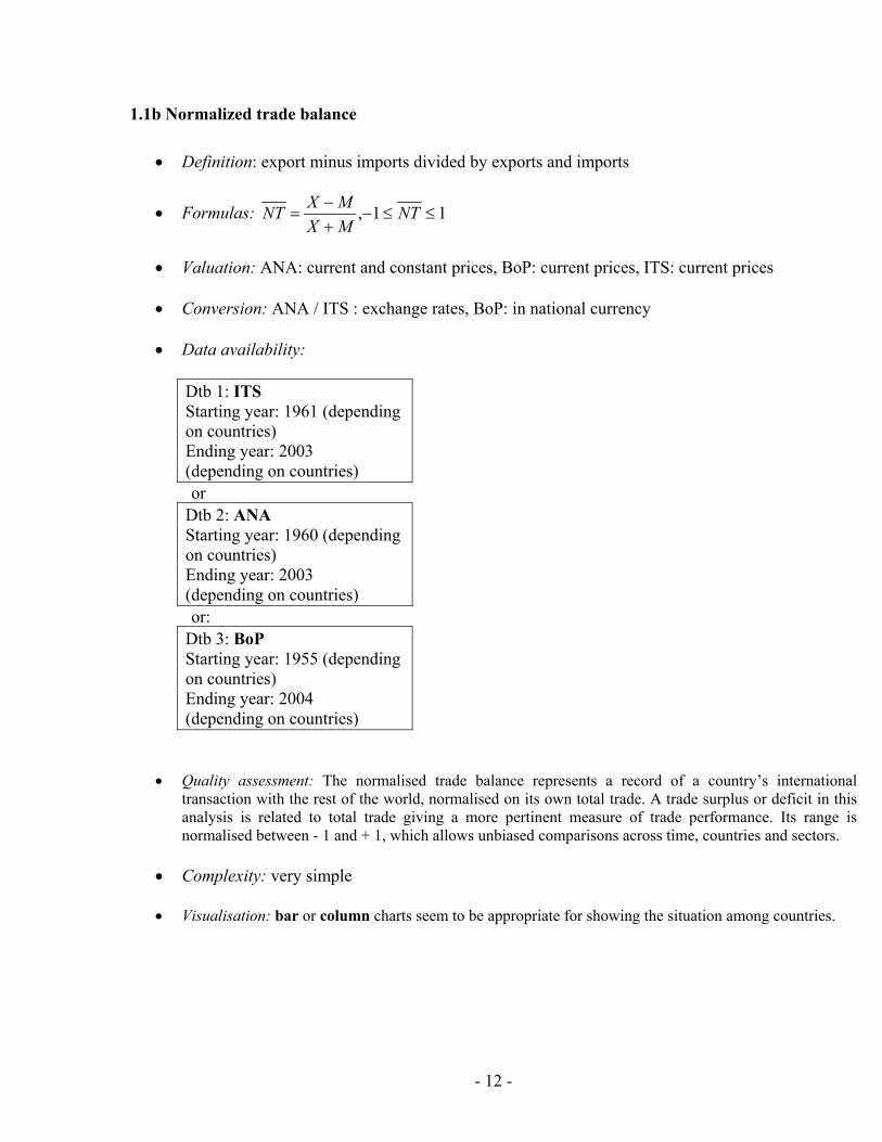
1.1b Normalized trade balance

• Definition: export minus imports divided by exports and imports

• Formulas: 11, ≤≤−+−

= NTMXMXNT

• Valuation: ANA: current and constant prices, BoP: current prices, ITS: current prices

• Conversion: ANA / ITS : exchange rates, BoP: in national currency




or: Dtb 3: BoP Starting year: 1955 (depending on countries) Ending year: 2004 (depending on countries)

• Quality assessment: The normalised trade balance represents a record of a country’s international transaction with the rest of the world, normalised on its own total trade. A trade surplus or deficit in this analysis is related to total trade giving a more pertinent measure of trade performance. Its range is normalised between - 1 and + 1, which allows unbiased comparisons across time, countries and sectors.



- 13 -

1.1c Coverage ratio

• Definition: The indicator shows exports as a percentage of imports

• Formulas:

100×=MXCR

If this percentage is < 100 %, the net trade balance will be negative (and vice versa). The coverage ratio is strictly related and substantially equivalent to the normalized trade

balance. The relationship between the two indicators is as follows: 11

+−

=CRCRNT

• Valuation: ANA (current and constant prices) or BoP (current prices) or ITS (current prices)

• Conversion: ANA / ITS : exchange rates, BoP : in national currency




or Dtb 3: BoP Starting year: 1955 (depending on countries) Ending year: 2004 (depending on countries)

• Quality assessment: The coverage ratio indicates if a country is more an exporting country or

more an importing country (in terms of value). The use of this indicator enables an unbiased comparison (ranking) between countries (in regards of their trade balances), sectors and periods.

- 14 -

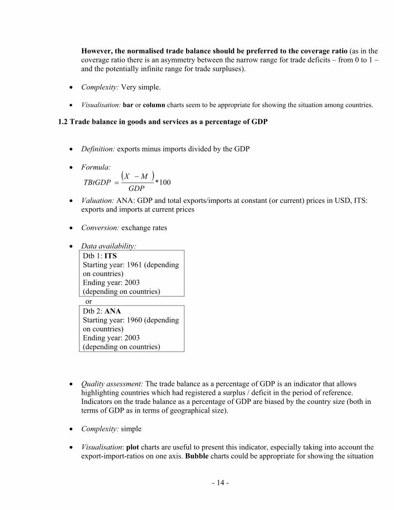
However, the normalised trade balance should be preferred to the coverage ratio (as in the coverage ratio there is an asymmetry between the narrow range for trade deficits – from 0 to 1 – and the potentially infinite range for trade surpluses).

• Complexity: Very simple.


1.2 Trade balance in goods and services as a percentage of GDP

• Definition: exports minus imports divided by the GDP

• Formula: ( )

100*GDP

MXTBtGDP

−=

• Valuation: ANA: GDP and total exports/imports at constant (or current) prices in USD, ITS: exports and imports at current prices

• Conversion: exchange rates




• Quality assessment: The trade balance as a percentage of GDP is an indicator that allows highlighting countries which had registered a surplus / deficit in the period of reference. Indicators on the trade balance as a percentage of GDP are biased by the country size (both in terms of GDP as in terms of geographical size).

• Complexity: simple

• Visualisation: plot charts are useful to present this indicator, especially taking into account the export-import-ratios on one axis. Bubble charts could be appropriate for showing the situation

- 15 -

among countries and regions with a focus on the size of GDP as third dimension (size of the bubbles).

Example:

United Kingdom

Spain

Slovak Republic

United States

Poland

Australia

HungaryCzech Republic

Finland

Sweden

Germany

Denmark

Netherlands

Canada

New ZealandIceland

Switzerland

Austria

Italy

France

Korea

OECD Average

0.5

0.8

1.1

1.4

-7 -2 3 8Trade Balance as a percentage of GDP

Export/ Import

%

Surplus

Deficit

Greece (-17.8,0.3)

Ireland(26.4,1.6)

Luxembourg(-10.9,0.8)

- 16 -

2. Trade openness 2.1 Trade-to-GDP-ratio

• Definition: The most frequently used indicator of the importance of international transactions relative to domestic transactions is the trade-to-GDP ratio, which is the the sum of exports and imports of goods divided by GDP. International trade tends to be more important for countries that are small (in terms of size or population) and surrounded by neighbouring countries with open trade regimes than for large, relatively self-sufficient countries or those that are geographically isolated and thus penalised by high transport costs. Other factors also play a role and help explain differences in trade-to-GDP ratios across countries, such as history, culture, (trade) policy, the structure of the economy (especially the weight of non-tradable services in GDP), re-exports and the presence of multinational firms (intra-firm trade).

• Formula: ( )

100*t

ttt GDP

XMT

+=

• Valuation: ANA: GDP and total exports/imports at constant (or current) prices in USD, ITS:

exports and imports at current prices





• Quality assessment: This widely used indicator measures a country’s “openness” or “integration” in the world economy. It represents the combined weight of total trade in its economy, a measure of the degree of dependence of domestic producers on foreign markets and their trade orientation (for exports) and the degree of reliance of domestic demand on foreign supply of goods and services (for imports). The trade-to-GDP ratio is often called the trade openness ratio. However, the term “openness” to international competition may be somewhat misleading. In

- 17 -

fact, a low ratio for a country does not necessarily imply high (tariff or non-tariff) obstacles to foreign trade, but may be due to the factors mentioned above, especially size and geographic remoteness from potential trading partners. Indicators on trade openness based on GDP are biased by the country size (both in terms of GDP as in terms of geographical size). It should be noted that this indicator may also expressed as average of exports and imports (not as the sum of both).


• Visualisation: bar or column charts seem to be appropriate for showing the situation among

countries. For more a more dynamic approach (time series), line charts can be used as well. Example:

0

20

40

60

80

100

120

140

160

180

200

2003 1995

- 18 -

2.2 Export propensity

• Definition: exports divided by GDP

• Formula: *

*

*Pr_

c

c

ct

tt GDP

XopX = c=country, t=time

• Valuation: ANA: GDP and exports at constant or current prices; ITS: exports at current prices.





• Quality assessment: Indicator which measures the exports by the size of the GPD of a country. However, this indicator is biased by the country size. It can be calculated for imports as well.

• Complexity: Very simple

• Visualisation: : bar or column charts seem to be appropriate for showing the situation among

countries. For more a more dynamic approach (time series), line charts can be used as well. Example:

- 19 -

01020304050607080

SLOVAK REPUBLIC

IRELAND

HUNGARY

CZECH REPUBLIC

NETHERLANDS

LUXEMBOURG

KOREA

FINLAND

SWEDEN

AUSTRIA

OECD Average

CANADA

SWITZERLAND

GERMANY

DENMARK

MEXICO

NEW ZEALAND

POLAND

ICELAND

FRANCE

SPAIN

ITALY

UNITED KINGDOM

AUSTRALIA

GREECE

UNITED STATES

CountryX/ GDP, M/ GDP (%) Goods 2003

IMPORT PROPENSITY EXPORT PROPENSITY

2.3 Import penetration ratio

• Definition: the import penetration ratio shows to what degree domestic demand is satisfied by imports.

• Formula: DMIP = M = Imports, D= Domestic Demand

where the domestic demand is the difference between the GDP and the net exports (exports- imports) [D = GDP-X+M)].

• Valuation: ANA: constant prices or current prices, ITS: current prices.



Dtb 1: ANA Starting year: 1960 (depending on countries) Ending year: 2003 (depending on countries)

or: Dtb 2: ITS Starting year: 1960 (depending on countries) Ending year: 2003 (depending on countries)

- 20 -

• Quality assessment: The import penetration rate shows the degree of domestic demand satisfied

by imports. It represents a measure of the importance of imports in the domestic economy, either by sector or overall, usually defined as the value of imports divided by the value of apparent consumption that is domestic production plus imports minus exports, sometimes also adjusted for changes in inventories. This indicator, hence, measures the dependence of a country’s domestic demand on imports. A low penetration rate does not necessarily imply import barriers. It may by example reflect greater price competitiveness on the part of national firms and/or can be biased by the country size/geography.

• Complexity: Simple

• Visualisation: : bar or column charts seem to be appropriate for showing the situation among

countries. For more a more dynamic approach (time series), line charts can be used as well.

0

10

20

30

40

50

60

70

80

90

100

LUXEM

BOURG

BELGIUM

IRELAND

SLOVAK

REPUBL

IC

NETHERLA

NDS

CZECH REP

UBLIC

HUNGARY

AUSTR

IA

OECD Aver

age

CANADA

SWITZ

ERLA

ND

SWED

EN

NEW ZE

ALAN

D

PORTU

GAL

NORWAY

KOREA

ICELAND

DENMAR

K

FINLA

ND

GERMAN

YITA

LY

UNITED KI

NGDOM

GREECESPA

IN

TURKE

Y

POLAND

FRAN

CE

AUSTRALIA

MEXICO

UNITED ST

ATES

JAPAN

Country

Import Penetration

1995 2003

Luxembourg (118,163)

2.4 Trade per capita

• Definition: Trade volume (exports and imports) divided by the number of inhabitants

• Formula: ( )Ninhab

MXTc +=

Where Ninhab = Number of inhabitants

• Valuation: ANA: constant prices or current prices, ITS: current prices.


- 21 -




and Dtb 3: ALFS Starting year: 1955 (depending on countries) Ending year: 2003 (depending on countries)

• Quality assessment: Measuring the trade volume of a country per inhabitant provides a rough standard measure of the magnitude of trade per capita.



countries. For more a more dynamic approach (time series), line charts can be used as well. Bubble charts can be used too, e.g. for comparing two reference years (X-/Y-axis) with a focus on the number of inhabitants or GDP as third dimension (size of the bubbles).

- 22 -

3. Trade performance indicators 3.1. Market shares

• Definition: exports or imports of a country as share of total exports or imports of the region/world.

• Formula:

a - Share of exports: 10,

1

≤≤=

∑=

Xin

ii

iXi S

X

XS

b - Share of imports: 10,

1

≤≤=

∑=

Min

ii

iMi S

M

MS

Where i=1…n countries of the region/world

• Valuation: ANA: constant or current prices; ITS: current prices




or: Dtb 2: ANA Starting year: 1960 (depending on countries) Ending year: 2003 (depending on countries)

• Quality assessment: An indicator to measure the degree of importance of a country on the total

trade of the respective region.


- 23 -

• Visualisation: usually pie charts are appropriate for visualizing market shares, depending on the number of countries to be displayed. The total pie (100 %) represents the total market volume of the respective market (region/world).

Example:

Other OECD member countries, 14.5

SWITZERLAND, 2.0

NETHERLANDS, 4.5

UNITED STATES, 20.2

GERMANY, 10.9

JAPAN, 10.1

UNITED KINGDOM, 7.6

FRANCE, 6.6CANADA, 5.7

ITALY, 6.5

KOREA, 2.6

BELGIUM, 3.8

SWEDEN, 1.9

MEXICO, 2.4

SPAIN, 2.7

3.2 Export performance

• Definition: Export performance is the ratio between export volumes and export markets for total goods and services. The calculation of export markets is based on a weighted average of import volumes in each exporting country’s markets, with weights based on trade flows in 2000.

• Formula: MX ti

n

ii

tc

tcEP ∆∑∆

=

−=1α

• where:

X tc∆ / M t

i∆ : export growth rate of the country c in period t / import growth rate of the market i in period t

α i : weight of market i for country c in period

• Valuation: ANA: constant or current prices, ITS: current prices



- 24 -



• Quality assessment: Indicator to relate export growth rates to the import dynamics of the

markets/regions.

• Complexity: simple on aggregated level. • Visualisation: bar or column charts seem to be appropriate for showing the situation among

countries and regions. 4. Geographic concentration indicators 4.1. Herfindahl index of geographical concentration

• Definition: The Herfindahl index of geographical concentration for country A’s exports is the sum of the squares of the market shares held in each country of destination i, i.e.:

• Formula:

∑

∑=

== n

ii

iH

X

Xn

i

1

2

1

Where i=1…n countries of destination

- 25 -

If each of the n countries of destination received the same export value, the Herfindahl index

would be equal to: n

H 1=

• Valuation: Exports FOB, current prices



Dtb: ITS Starting year: 1961 (depending on countries) Ending year: 2003 (depending on countries)

• Quality assessment: The Herfindahl index indicates the geographical concentration of a country’s exports or imports. However, the concentration can vary markedly by commodity or type of goods. It can be calculated for imports as well. The inverse of the Herfindahl index (“equivalent number”) can be used for measuring the degree of diversification of a country.

• Complexity: Medium. The lower the market shares are, the more negligible their values would

be, and the calculations could disregard them.

• Visualisation: Depending on the number of reference years and/or countries used (trends/benchmarking), plots or columns seem to be good options to visualise this indicator. Bubble charts might be used as well.

Examples:

- 26 -

Country A

Country H

Country J

Country I

Country E

Country D

Country F

Country C

Country G

Country B

0.0

0.1

0.2

0.3

0.4

0.5

0.6

0.7

0.8

0.9

1.0

0.0 0.1 0.2 0.3 0.4 0.5 0.6 0.7 0.8 0.9 1.01995

2003

0.00.10.20.30.40.50.60.70.80.91.0

Country A

Co untry B

Co untry C

Country D

Co untry E

Co untry F

Country G

Country H

Co untryI

Co untry J

Co untry K

19952003

Note: Hypothetical values 4.2 Geographical distribution of export market shares of goods

• Definition: exports of the country to the region, divided by OECD’s total exports to that region

• Formula: trOECD

trct

pc XX

GDX,

,, *100=

where:

trcX , : exports of the country c to the region r for the year t

trOECDX , ; OECD’s total exports to that region for the year t.

• Valuation: Imports and exports at current prices




- 27 -

• Quality assessment: The geographical distribution of export market shares of goods gives an insight into the importance of exports of individual member countries within OECD’s total exports to selected regions

• Complexity: simple • Visualisation: bar or column charts seem to be appropriate for showing the situation among

countries and regions. Example:

0.0 2.0 4.0 6.0 8.0 10.0

Ger many

Fr ance

Belgium

United Kingdom

Nether lands

Italy

Uni ted States

Spain

Japan

Switzer land

Ir eland

Sweden

Austr ia

Nor way

Denmar k

Poland

Czech Republ ic

Hungar y

Finland

Por tugal

Kor ea

Tur key

Canada

Slovak Republ ic

Austr al ia

Luxembour g

Gr eece

Mexico

New Zealand

Iceland

1995 2003

4.3 Geographical distribution of import penetration of goods

• Definition: exports of the country to the region of destination, divided by the domestic demand of the region of destination

• Formula: tr

trct

pc ddX

GDIP ,, *100=

where:

trcX , : exports of the country c to the region r for the year t trdd ; domestic demand of the region of destination for the year t.

• Valuation: current prices


- 28 -



• Quality assessment: The geographical origin of import penetration of goods shows the role of the import trading partners – and the imports themselves - for the total domestic demand of the country.

• Complexity: simple • Visualisation: bar or column charts seem to be appropriate for showing the situation among

countries and regions. Example:

0 5 10 15 20

Germany

France

BelgiumUnited Kingdom

NetherlandsItaly

United States

SpainJapan

Sw itzerlandIreland

Sw eden

AustriaNorw ay

DenmarkPoland

Czech Republic

HungaryFinland

PortugalKorea

Turkey

CanadaSlovak Republic

AustraliaLuxembourg

Greece

MexicoNew Zealand

Iceland

2003 1995

4.4 Services trading partners (exports/imports)

• Definition: exports/imports of the country/countries to/from the region, divided by the total exports/imports of the region.

- 29 -

• Formula: tr

trct

rc XX

XMSs ,, *100= or t

r

trct

rc MM

IMSs ,, *100=

where:

trcXMSs , / t

rcIMSs , : export/import market share (services) of country c within region r in the year t

trcX , / t

rcM , : exports/imports of the country c to the region r for the year t trX / t

rM ; total exports/imports of services of the region for the year t.




Dtb: TIS Starting year: 1992 (depending on countries) Ending year: 2002 (depending on countries)

• Quality assessment: Useful indicator to show the importance of import/export partner countries for the trade in services of the concerned region(s).

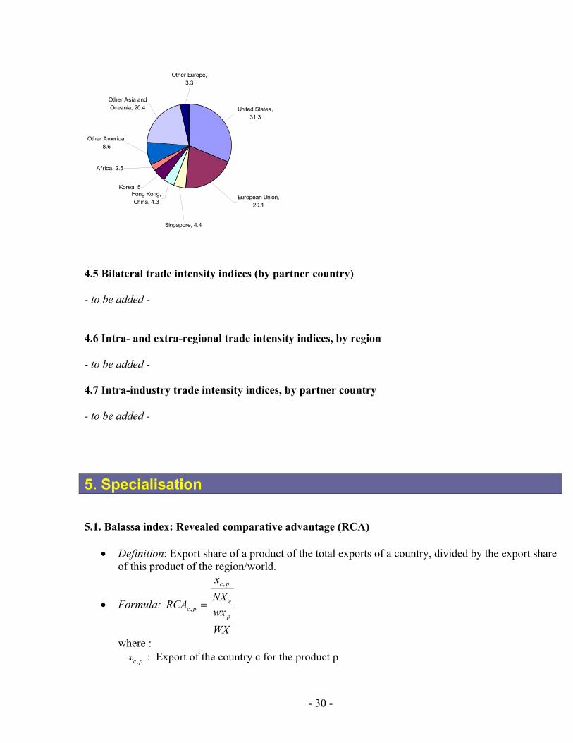
• Complexity: simple • Visualisation: usually pie charts are appropriate for visualizing market shares, depending on the

number of countries to be displayed. The total pie (100 %) represents the total market volume of the respective market (region/world).

. Example:

- 30 -

United States, 31.3

European Union, 20.1

Singapore, 4.4

Hong Kong, China, 4.3

Korea, 5

Africa, 2.5

Other America, 8.6

Other Asia and Oceania, 20.4

Other Europe, 3.3

4.5 Bilateral trade intensity indices (by partner country) - to be added - 4.6 Intra- and extra-regional trade intensity indices, by region - to be added - 4.7 Intra-industry trade intensity indices, by partner country - to be added - 5. Specialisation 5.1. Balassa index: Revealed comparative advantage (RCA)

• Definition: Export share of a product of the total exports of a country, divided by the export share of this product of the region/world.

• Formula:

WXwxNXx

RCAp

c

pc

pc

,

, =

where : pcx , : Export of the country c for the product p

- 31 -

cNX : Total (national) exports of the country c

pwx : Total exports for the world (OECD) for the product p WX : Total exports for the world (OECD)

If it takes a value less than 1, this implies that the country is not specialised in exporting the product. The share of product p in country i exports is less than the corresponding world share. Similarly, if the index exceeds 1, this implies that the country is specialised in exporting the item.





• Quality assessment: The Balassa index measures the intensity of trade specialisation of a country within a region or the world. In general practice, RCA indices should be only used in product categories where trade is not distorted by export incentives and trade barriers, because they are likely to obscure whether a country has a real comparative advantage or disadvantage in these goods.

• Complexity: Medium. • Visualisation: bar or column charts seem to be appropriate for showing the situation among

countries and regions.

- 32 -

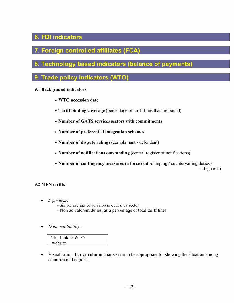
6. FDI indicators 7. Foreign controlled affiliates (FCA) 8. Technology based indicators (balance of payments) 9. Trade policy indicators (WTO) 9.1 Background indicators

• WTO accession date

• Tariff binding coverage (percentage of tariff lines that are bound)

• Number of GATS services sectors with commitments

• Number of preferential integration schemes

• Number of dispute rulings (complainant - defendant)

• Number of notifications outstanding (central register of notifications)

• Number of contingency measures in force (anti-dumping / countervailing duties / safeguards)

9.2 MFN tariffs

• Definitions: - Simple average of ad valorem duties, by sector - Non ad valorem duties, as a percentage of total tariff lines


Dtb : Link to WTO website


countries and regions.

- 33 -

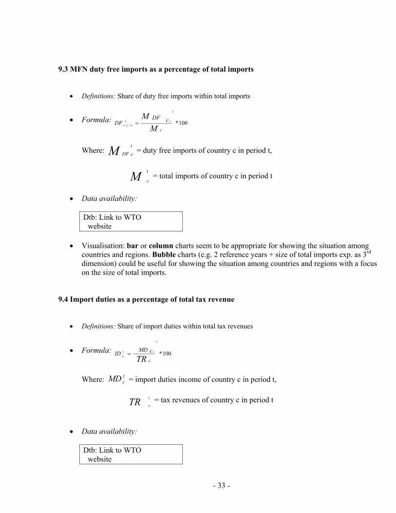
9.3 MFN duty free imports as a percentage of total imports

• Definitions: Share of duty free imports within total imports

• Formula: 100*/,

t

C

ctoic M

M cDFDF =

Where: t

cDFM = duty free imports of country c in period t,

t

cM = total imports of country c in period t


Dtb: Link to WTO website


countries and regions. Bubble charts (e.g. 2 reference years + size of total imports exp. as 3rd dimension) could be useful for showing the situation among countries and regions with a focus on the size of total imports.

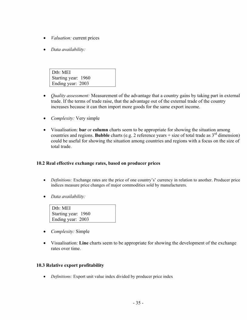
9.4 Import duties as a percentage of total tax revenue

• Definitions: Share of import duties within total tax revenues

• Formula: 100*,

t

C

ctc TR

MD cID =

Where: t

cMD = import duties income of country c in period t,

t

cTR = tax revenues of country c in period t



- 34 -

• Visualisation: Bubble charts (e.g. 2 reference years + size of total imports exp. as 3rd dimension) can be appropriate for showing the situation among countries and regions with a focus on the size of total tax income. Bar or column charts can be used as well.

9.5 Import duties as a percentage of total merchandise imports

• Definitions: Share of import duties within total merchandise imports

• Formula: 100*,

t

C

ctc M

MD cIDr =

Where: t

cMD = import duties income of country c in period t,

t

cM = merchandise imports of country c in period t



• Visualisation: Bubble charts (e.g. 2 reference years + size of total imports exp. as 3rd dimension)

can be appropriate for showing the situation among countries and regions with a focus on the size of total merchandise imports. Bar or column charts can be used as well.

10. Price indicators 10.1 Terms of trade

• Definitions: Terms of trade is the ratio of export and import prices.

• Formula: 100*

t

M

ctc P

P xTT =

Where: xP = price index, exports

MP = price index, imports

- 35 -



Dtb: MEI Starting year: 1960 Ending year: 2003

• Quality assessment: Measurement of the advantage that a country gains by taking part in external

trade. If the terms of trade raise, that the advantage out of the external trade of the country increases because it can then import more goods for the same export income.

• Complexity: Very simple


countries and regions. Bubble charts (e.g. 2 reference years + size of total trade as 3rd dimension) could be useful for showing the situation among countries and regions with a focus on the size of total trade.

10.2 Real effective exchange rates, based on producer prices

• Definitions: Exchange rates are the price of one country’s’ currency in relation to another. Producer price

indices measure price changes of major commodities sold by manufacturers.


Dtb: MEI Starting year: 1960 Ending year: 2003


• Visualisation: Line charts seem to be appropriate for showing the development of the exchange

rates over time. 10.3 Relative export profitability

• Definitions: Export unit value index divided by producer price index

- 36 -

• Formula: 100*

t

ctc PP

UV xEP =

Where: xUV = unit value index (exports)

PP = producer price index

• Data availability: unit value indices are not available for all member countries.

Dtb 1: MEI Starting year: 1960 Ending year: 2003


• Quality assessment: Measurement of the degree of profitability of exports.



countries and regions. Bubble charts (e.g. 2 reference years + size of total trade as 3rd dimension) could be for showing the situation among countries and regions with a focus on the size of total trade.

11. Trade intensity and specialisation indicators Chapter to be further developed in the 2nd phase of the TIP.

Trade and Globalisation Statistics Section (TAGS) Lima 2007/background document… · - 1 - united...

Documents

Transcript of Trade and Globalisation Statistics Section (TAGS) Lima 2007/background document… · - 1 - united...