Thammasat Int. J. Sc. Tech.. Vol. 10. No. 4. Ocrober-December 2005

Traction Control of a Rocker-BogieField Mobile Robot

Mongkol Thianwiboon and Viboon SangveraphunsiriRobotics & Automation Laboratory, Deparlment of Mechanical Engineering

Chulalongkom University, Phayathai Rd., Pathum Wan, Bangkokkiene(Zleng. chula. ac. th, viboon. s(raeng. chula. ac.th

AbstractA method for kinematics modeling of a six-wheel Rocker-Bogie mobile robot is described in

detail. The forward kinematics is derived by using wheel Jacobian matrices in conjunction with wheel-ground contact angle estimation. The inverse kinematics is to obtain the wheel velocities and steeringangles from the desired forrr"'ard velocity and turning rate of the robot. Traction Control is alsodeveloped to improve traction by comparing information from onboard sensors and wheel velocities tominimize slip of the wheel. Finally, a small robot is built and tested in various conditions of surfacesincluding verlical obstacle, inclined surface and uneven terrain outdoor conditions.

Keywords: Rocker-Bogie Suspension / Traction Control / Slip Ratio

l. IntroductionThe effectiveness of a wheeled mobile

robot has been proven by NASA by sending asemi-autonomous rover "Sojourner" whichlanded on Martian surface in 1997[1]. Futurefield mobile robots are expected to traversemuch longer distance over more challengingterrain than Sojourner, and perform moredifficult tasks. Other examples of rough terrainapplications for robots can be found inhazardous material handling applications, suchas explosive ordnance disposal, and search andrescue.

Corresponding to such growing attention,the researches vary from mechanical design,performance of the robot, control systems,navigation system, path planning, field tests, andso on.

However, there are very few a dynamics ofthe robot. This is because the field robots areconsidered too slow to encounter a dynamiceffect. And the high mobility of the robot,moving in 3 dimensions with 6 degrees offreedom (X, Y, Z, pitch, yaw. ro11), makes thekinematics modeling a more challenging taskthan the robots which move on flat and smoothsurfaces (3 degrees of freedom: X, Y, rotationabout Z axis)

In rough terrain, it is critical for mobilerobots to maintain maximum traction. Wheelslip could cause the robot to lose control and betrapped. Traction control for low-speed mobilerobots on flat terrain has been studied by Reisterand Unseren [2] using pseudo velocity tosynchronize the motion of the wheels duringrotation about a point. Sreenivasan and Wilcox[3] have considered the effects of terrain ontraction control by assuming knowledge ofterrain geometry, soil characteristics and real-time measurements of wheel-ground contactforces. However, this information is usuallyunknown or difficult to obtain directly. Quasi-static force analysis and a fuzzy logic algorithmhave been proposed fbr a rocker-bogie robot [4].

Knowledge of terrain geometry is critical tothe traction control. A method for estimatingwheel-ground contact angles using only simpleon-board sensors has been proposed [5] Amodel of load-traction factors and slip-basedtraction has been developed [6]. The travelingvelocity of the robot is estimated by measuringthe PWM duty ratio driving the wheels. Angularvelocities of the wheels are also measured andthen compared with estimated traveling velocityto estimate the slip and perform a tractioncontrol loop.

48

In this research work, a small six-wheelrobot with Rocker-Bogie suspension isdesigned, built and tested. The method to derivemathematical modeling such as, the wheel-ground contact angle estimation and kinematicsmodeling is also described. Finally, a tractioncontrol system is developed and implemented onthis robot.

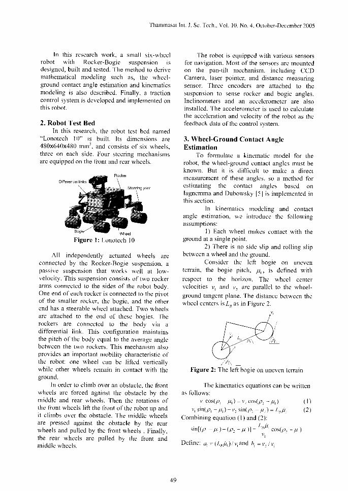
2. Robot Test BedIn this research, the robot test bed named

"Lonotech 10" is built. Its dimensions are480x640x480 mm3, and consists of six wheels,three on each side. Four steering mechanismsare equipped on the front and rear wheels.

All independently actuated wheels areconnected by the Rocker-Bogie suspension, apassive suspension that works well at low-velocity. This suspension consists of two rockerarms connected to the sides of the robot body.One end ofeach rocker is connected to the oivotof the smal ler rocker . the bogie. and the otherend has a steerable wheel attached. Two wheelsare attached to the end of these bogies. Therockers are connected to the body via adifferential link. This configuration maintainsthe pitch of the body equal to the average anglebetween the two rockers. This mechanism alsoprovides an impoftant mobility characteristic ofthe robot: one wheel can be lifted verticallywhile other wheels remain in contact with theground.

In order to climb over an obstacle. the frontwheels are forced against the obstacle by themiddle and rear wheels. Then the rotations olthe front wheels lift the front of the robot up andit climbs over the obstacle. The middle wheelsare pressed against the obstacle by the rearwheels and pulled by the front wheels . Finally,the rear wheels are pulled by the front andmiddle wheels.

Thammasat Int. J. Sc. Tech.. Vol. 10. No. 4, Ocrober-December 2005

The robot is equipped with various sensorsfor navigation. Most of the sensors are mountedon the pan-ti lt mechanism, including CCDCamera, laser pointer, and distance measuringsensor. Three encoders are attached to thesuspension to sense rocker and bogie angles.Inclinometers and an accelerometer are alsoinstalled. The accelerometer is used to calculatethe acceleration and velocity of the robot as thefeedback data of the control system.

3. Wheel-Ground Contact AngleEstimation

To formulate a kinematic model for therobot, the whecl-ground contact angles must beknown. But it is difficult to make a directmeasurement of these angles, so a method forestimating the contact angles based onIagnemma and Dubowsky [5] is implemented inthis section.

In kinematics modeling and contactangle estimation, we introduce the followingassumptlons:

I ) Each wheel makes contact with theground at a single point.

2) There is no side slip and roll ing slipbetween a wheel and the ground.

Consider the left bogie on uneventerain, the bogie pitch, trt,, is defined withrespect to the horizon. The wheel centervelocities r,, and r,, are parallel to the wheel-ground tangent plane. The distance between thewheel centers isl, as in Figure 2.

1i:',Figure 2: The left bogie on uneven terrain

The kinematics equations can be writtenas follows:

u, cos(p, l\) : vz cos(p. - 1t,) ( I )u, sin(p, lt,) - r. sin(p. - lt.) = Lo!, Q)

Combining equation ( l) and (2):

s i n [ rp , F l - ( 1 t . l t , l l = Lo l t t

cos {p . - p , )vt

Def ine : a , : (Lo1. t , ) l v ,and b , = r , , / v ,

Figure l: Lonotech l0

49

Thammasat Int. J. Sc. Tech., Vol 10. No. 4. October-December 2005

( - : - h ) \

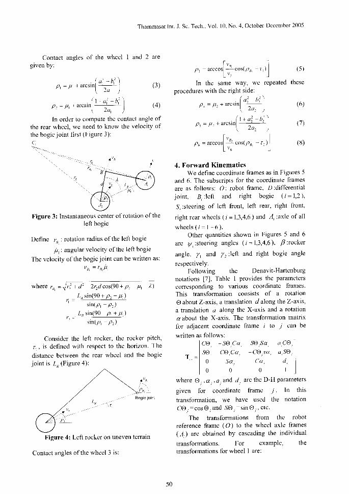
pt = Ft + arcsinl "r--- t (3 )

\ 2 o , ) "

/ ' ) ' r \. l l l d , - h , - I

P : = F t + a r c s l n { 4 }\ 2 o , ) "

ln order to compute the contact angle of

the rear wheel, we need to know the velocity of

the bogie joint first (Figure 3):

cr\ - . - .

Contact angles of the wheel I and 2 ategiven by:

at''

Figure 3: Instantaneous center ofrotation oftheleft bogie

Define rB, : rotation radius of the left bogie

it,: angular velocity ofthe left bogie

The velocity of the bogie joint can be written as:V a = f u / l t

. -where ru = ,lr: + d' 2rr./cos{90 + p:- Ft ))

l , s in(90 + Pz - 11,)sin(P, - P')

Lo sin(90 P, + 11.\' t = - , in1o, - p;

Consider the left rocker, the rocker pitch,

r, , is defined with respect to the horizon. The

distance between the rear wheel and the bogiejoint is I* (Figure 4):

1 v a

Pa

Bogie jornt

Figure 4: Left rocker on uneven terrain

Contact ansles of the wheel 3 is:

["u, . lp, =arccosl rcos(P, , - r ) ] (5)

In the same way, we rePeated theseprocedures with the right side:

p, = tt:* ur.rinf '+t'l (6)\ ' " 2 /

. ( t - " i - r : )p . = p . l a r c s l n l t t l

, 2o. )

o. = -".or[L.o<p,. - r,l]

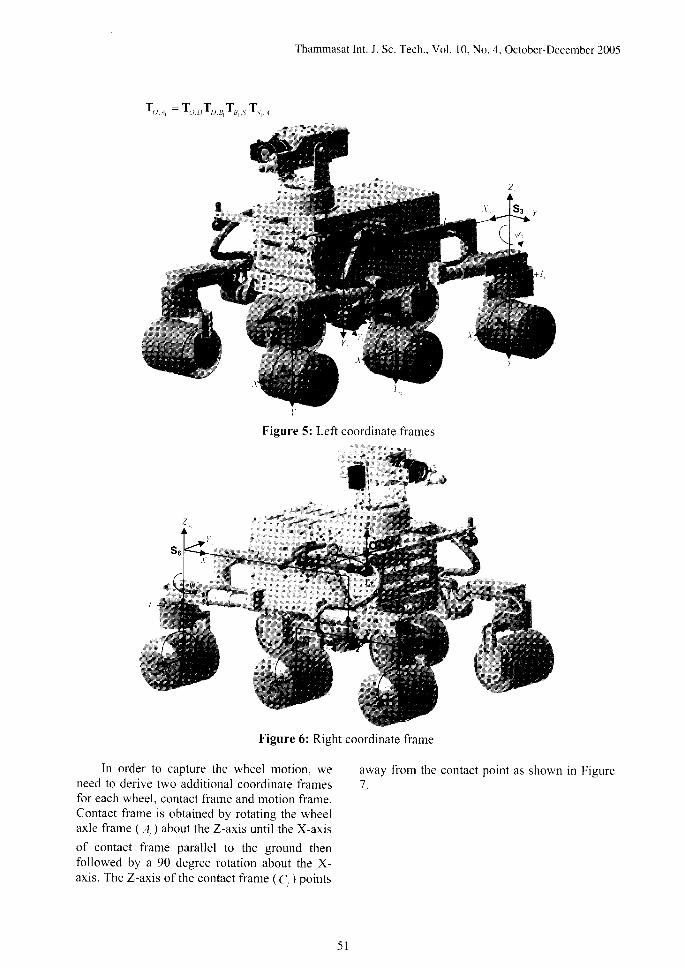
4. Forward KinematicsWe define coordinate frames as in Figures 5

and 6. The subscripts for the coordinate framesare as follows: O: robot frame, D :differentialjoint, B, : left and right bogie (i =1,2),

S,:steering of left front, left rear, right front,

right rear wheels (i = 1,3,4,6) and A,:axle of all

w h e e l s ( t = l - 6 ) .Other quantities shown in Figures 5 and 6

are r!./ :steering angles (I =1,3,4,6 ), p:rocker

angle, y, and yr:left and right bogie angle

respectively.Following the Denavit-Hartenburg

notations [7], Table I provides the parameterscorresponding to various coordinate frames.This transformation consists of a rotation

@ about Z-axis, a translation d along the Z-axis,

a translation a along the X-axis and a rotation

a about the X-axis. The transformation matrix

for adjacent coordinate frame i to jr can be

written as follows:

(8)

lti;,

where

given for coordinate frame i In this

transformation. we have used the notation

CO, :cos@, and S@, -s in O, , etc .

The transfomations from the robotreference frame (O) to the wheel axle frames( A,) are obtained by cascading the individual

transformations. For examPle, thetransformations for wheel I are:

1 . " s o c a s o s a l l c o l

l s o , C o C a C o s a a S o I: l o sa, Co, di

Il 0 0 0 I l

@,, a,, a, and d, are the D-H Parameters

50

Thammasat Int. J. Sc. Tech., Vol. 10. No. 4. October-December 2005

To.,, =TnlT,,. , Tr., Tr,. .r ,

',

In order to capture the wheel motion, weneed to derive two additional coordinate framesfor each wheel. contact frame and motion frame.Contact frame is obtained by rotating the wheelaxle frame ( l, ) about the Z-axis until the X-axis

of contact frame parallel to the ground thenfollowed by a 90 degree rotation about the X-axis. The Z-axis of the contact frame ( C, ) points

away from the contact point as shown in Figure7 .

5 t

Figure 5: Left coordinate frames

Figure 6: Right coordinate frame

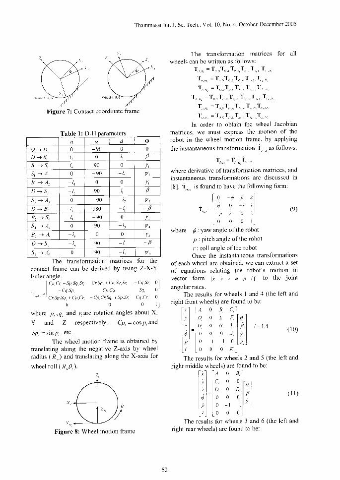
Figure 7: Contact coordinate frame

Table l: D-H

The transformation matricescontact frame can be derived by usingEuler angle.

where p, ,q, and / are rotation angles about X,

Y and Z respectively. Cp, =cosp and

S P = s i n p ' e t c '

The wheel motion frame is obtained bytranslating along the negative Z-axis by wheelradius ( R. ) and translating along the X-axis for

wheel ro l l (R"0,)

X,

X,,

I cp c, sp sq s, Cr,Sp, + Cp,Sq ,Sr, - Cq Sr

_ I - ( q , 5 1 ' C p t q 5 4T . . = l

lCr,Sp,Sq,+(-p,Cr, Cp,Cr,Sq,+SP,Sr, Cq,Cr,

0 0 0

Thammasat Int. J. Sc. Tech., Vol. 10, No. 4, October-December 2005

The transformation matrices for all

wheels can be written as follows:

Tn,, =T,,, ,T n o Tr,. , T-,T,,. , I .u

l , .rr , = T,,.rTr., Tr., ,T,, . , .1,, , ,

T,, .u. = T,,.rT,, r ,1.. , ,T,, . , 'T,, u,

1,., , , , - l , .r ,Tr.r,To,.r,T,, uT,,. , .1, , , ,

T,r. ,u. : T,, . t1,. , , ,Tu.., .T,. . , .T,, .r .

1,. , , , = l , . , ,Tn r^Trn. ' , .T,n., ^T,,, .u,.

In order to obtain the wheel Jacobian

matrices, we must express the motion of the

robot in the wheel motion frame, by applying

the instantaneous translormation f , , as fol lows:

for theZ-X-Y

T , , , t = T u i , , T r , ,

where derivative of transformation matrices, andinstantaneous transformations are discussed in

[8]. Tr,, is found to have the following form:

I q o i ' r ]r , n

l ' l l , n ,P T U - -

[ o o o r ] ]

where Q: yaw angle ofthe robot

p : pitch angle of the robot

r: roll angle ofthe robotOnce the instantaneous transformations

of each wheel are obtained, we can extract a setof equations relating the robot's motion invector form ti _i ; d p i'l' to the joint

angular rates.The results for wheels I and 4 (the left and

right front wheels) are found to be:

[ r ] l t o B . , l_ _l r L l a o E , , l ' , ), l = o 0 H , l p i t . 4 ( t 0 )

l 0 l l o o o t l r ll p l 0 - 1 - r 0 l l i ILul lo o o K,l-The results for wheels 2 and 5 (the left and

right middle wheels) are found to be:

['l lo, : i']j ' l l c o o l t r t

l : l = l ? I i l l p l ( , ' )l d l o o u l l nl r l o - 1 r L ' ' rl i l [ 0 o 0 ]

The results for wheels 3 and 6 (the left andright rear wheels) are found to be:

a a f, @

o > D 0 - 9 0 0 0D - + 8 , I 0 ll n

B , + S , I 90 0 Tt

S, -+ l, 0 90 - t, Vt

B, --> A. 0 0 /t

D - + S , - l(, 90 I p

S, -+ l, 0 - 9 0 - t V:

D - + 8 . l) 1 8 0 - l l _ B

B, -+ S, l" - 9 0 0 T:S, --+ ,40 0 90 - t Vt

B. -+ A, - /s 0 0 T:

D - + S n 90 - t _ B

J,. --+ /" 0 90 - t Va

52

Figure 8: Wheel motion frame

Thammasat Int. J. Sc. Tech.. Vol. 10. No. 4. October-December 2005

[ . ] I , r o , ll i l l c , o , l t a )' , . 1 u ^ l i l l p l ( t 2 )d l 0 0 G , l l

' . I

, l l o - r o l L Y l

L i l L 0 0 H , )

is the angular velocity of the wheel,rocker pitch rate, j'is the bogie pitch

rpi.is the steering rate of the steerable

i = A A + R i + C u

Q " = J vThe rolling velocities of the front wheels can bewritten as:

r,-t, i -?i,,

(14 )

, = 1 ,3 (15)where d

B ls the

rate and

wheel.The parameter A and K, in the matrices

above can be easily derived in terms of wheel-ground contact angle (p,..p) and joint angle

( 0,y and ry ). For example, the parameter Arof

the front left wheel is:

A , = - l * G ( \ t y , t \ c p ' G r v S v ' l\ - t + s \ t p r ) r

+ sptsvt)(200 - 400Cp,Sp, + 200C1 p,s'�p)l

It is seen that these set of equations arein the general form:

u = J , 4 , i = l - 6 ( 1 3 )

where J, is the Jacobian matrix of wheel i , and

q, is the joint angular rate vector.

We will see that the 5th equation (5throw) does not contribute to any unknowns. Itsimply states that the change in pitch is equal tothe change in the bogie and rocker angles. Withthe help of an installed inclinometer, p can be

sensed without knowledge of the rocker andbogie angles. Since only the fu, in equation (10)

to (12) . conta ins i , and p. we can e l iminate

them from further consideration.

5. Inverse KinematicsThe purpose of inverse kinematics is to

determine the individual wheel rolling velocitieswhich will accomplish desired robot motion.The desired robot motion is given by forwardvelocity and turning rate. In this section, we willdevelop all 6 wheels rolling velocities with ageometric approach to determine steering angleof steerable wheels.5.1 Wheel Rolling Velocities

Consider the forward kinematics of thefront wheel (10). Define the desired forwardvelocity as i,., and desired heading angular rate

asl,/. From equation (10), the first and the

fourth equation give:

0 =

Similarly, the rolling velocities of the middlewheels can be written as:

(16 )

Finally the rolling velocities of the rear wheelscan be written as

D- D ,

x , - r A ,

^ " G ' " ( t 7 )

A * i = J , 6, A ,

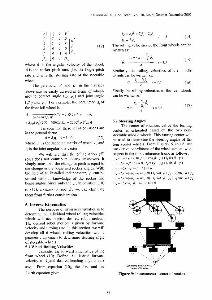
5.2 Steering AnglesThe center of rotation, called the turning

center, is estimated based on the two non-steerable middle wheels. This turning center willbe used to determine the steering angles of thefour corner wheels. From Figures 5 and 6, wecan derive coordinates of the wheel centers withrespect to the robot reference frame as follows:-{(.r = /, cos / + /r sin B + /. cos(/ - y,) + l,sin( B - y,)

x c. z = I " cos /J + I tsin B * 1, cos(/ - y,) + I,sin( p - y,)r , . - - i ^ c o s / + ( 1 , t l , ; s i n P

:rc.r = i: cos(-/) - /, sin(-p) + /. c os(- B + y.) + l,sin(- B + y.)

;r.. = /, cos(-p) - /, sin(-/) - 1, cos(-B + 7' ) + /r sin(- B + y')

rco = -/e cos(-/) - (i + 1. ) sin /

^ i, - 8.i,.H = " " ' t = 2 . )' A

Estimated Instantaneous

53

Figure 9: Instantaneous center ofrotation

Thammasat Int. J. Sc. Tech.. Vol 10, No. 4. Oclober-December 2O05

From figure 9, the instantaneous center ofrotation can be estimated by averaging the xposition of the middle wheels. The distancealong the Z-axis is neglected because there isonly I degree of freedom per each steering. I1'the wheel's axis is steered to intersect with thecenter of rotation on the X-axis, the angle in theZ direction is coupled and cannot be controlled.

Using the estimated center of rotation, thedesired steering angle for each steerable wheelcan be determined. Define R as a turning radius,x" is the distance in the X-direction of the center

of rotation with respect to the robot referenceframe, /, is the distance from the robot reference

frame to steering joint in the Y-direction (seeFigures 5 and 6). The desire steering angles are:

/ \ut, = arctanl

rc r - -rn I for wheel I

t R t , )

ur, = arctanl r, ' � tn

I lor wheel 3t R - 1 l

v, _ arcanl .r, r ra

I lor wheel 4t R t , )

,- - ur.,unl .r ' ̂ lro I ior wheel 6

I R - l l

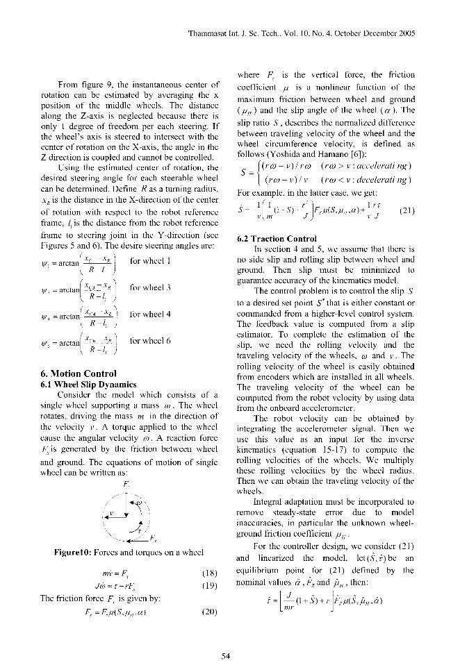
6. Motion Control6.1 Wheel Slip Dynamics

Consider the model which consists of asingle wheel supporting a mass m . The wheelrotates, driving the mass m in the direction ofthe velocity v. A torque applied to the wheelcause the angular velocity zo. A reaction force

{ is generated by the friction between wheel

and ground. The equations of motion of singlewheel can be written as:

F

Figurel0: Forces

m i = F ,

Jrb: r - rF,

The friction force { is given by:

F, = F.1t(S,pn,a)

where F.

coefficient

is the vertical force. the friction

p is a nonlinear function of the

maximum friction between wheel and ground(pn) and the slip angle of the wheel (a). The

slip ratio S, describes the normalized differencebetween traveling velocity of the wheel and thewheel circumference velocity, is defined asfollows (Yoshida and Hamano [6]):^ [V, - vl , rto \rat > v : attelerali ng )J = (

| (rt t v) u lrat < v: decelerul i ngI

For example, in the latter case, we get:. l 1 l r ' l l r r

S - ' l ' 1 l , S ) - ' . l F , 1 r l S . 1 r , t . c ( l + " ' ( 2 1 )v \ m . J I f , J

6.2 Traction ControlIn section 4 and 5. we assume that there is

no side slip and rolling slip between wheel andground. Then slip must be minimized toguarantee accuracy of the kinematics model.

The control problem is to control the slip Sto a desired set point S'that is either constant orcommanded from a higher-level control system.The feedback value is computed from a slipestimator. To complete the estimation of theslip, we need the rolling velocity and thetraveling velocity of the wheels, o and r,. Therolling velocity of the wheel is easily obtainedfrom encoders which are installed in all wheels.The traveling velocity of the wheel can becomputed from the robot velocity by using datafrom the onboard accelerometer.

The robot velocity can be obtained byintegrating the accelerometer signal. Then weuse this value as an input for the inversekinematics (equation l5-17) to compute theroll ing velocities of the wheels. We multiplythese rolling velocities by the wheel radius.Then we can obtain the traveling velocity of thewheels.

lntegral adaptation must be incorporated toremove steady-state error due to modelinaccuracies, in particular the unknown wheel-ground friction coefficient 4, .

For the controller design, we consider (21)

and l inear ized the model . le t 15. i1 be an

equilibrium point for (2 l) defined by thenominal values c? , F, and, pt, , then:

f r ^ 1 "t = | _1(1 + s) + r lF,p(s, 1t , , ,a)

l m r l

l * { 't \ r

J]!7

I/ T , . ' �

a " F ,

and torqueson a wheel

( 1 8 )

( l e )

(20)

54

The speed-dependent nominal linearizedslip dynamic is:

s - a(s - s; + 41, - t)+ h.o.t. Q2)

where a, and B, are linearization constants:

at= a [1 , , - s , . ! l ! ^ ! rs .p , , .a tl m J _ l . J

- | F ,p1s ,p*a1

Desfed Slrp Ralio

Rouot to t roo.uedo {ecKolrs

L l vF.o, ry * l_ legrcuor t 'a rdo ' ra lon

. d ( r . ) 0 , . ( 2 3 )' \ ' , = - l ( r - r )- v v

whereI r . 2 )

d $ ) = - l ' ( t * S . + x , ) + l r , p 1 r . + 5 . , t r t , , , a )L M J )

f r l �r = l "

l l r S ' ) - r l F , 1 t { S " . t r t n . a llmr j

It can be seen that (23) has an equilibrium point

g i ven by r : . - 0 , r= r - s i nce { (Q) :0 , and the

linearized slip model (22) with a pefturbationterm written as:

i .=?" . *LG- l l+ ' -L2 e4)where e,,(,t.) = QQ) - a,x.

Let the system dynamics (24) be augmentedwith a slip error integrator ir = S - S- : .r:

i i l i x lI " .

I l t v l . ] - ' '

i + B ( uXr r r - 1 - W (v t c , , ( x . llr: J lr: J

Thammasat lnt. J. Sc. Tech., Vol 10. No. .1. October-December 2005

/ J t : r l J

Define ,r: - S - S-, and assuming arbitrary

values of d,F, and lrrt , the wheel sliP

dynamics (21) can be written as:

' sleenng Ansle "t

., I St"".ng conror

Lsumalo_ '1

€339

' rracrion conror I

l]

l

Sensed Whee Ro l l rngS rp es lna lo ,

- T �

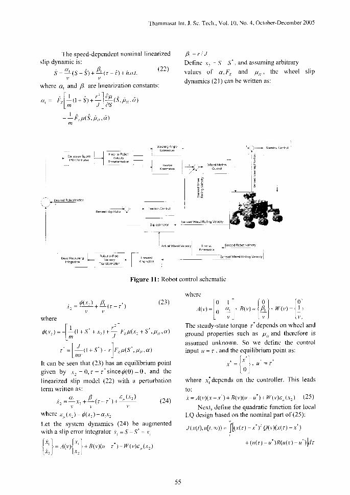
Figure 1l: Robot control schematic

where[ o l . ] f o l t o l

A \ v ) - ^ a , l . 4 1 " l = l P ' l " w o t - l t lu . . tL v l [ v J [ v J

The steady-state torque r'depends on wheel andground properties such as trt,,and therefore is

assumed unknown. So we define the controlinput r.r = r, and the equilibrium point as:

' l x ' Ix = i l . u = r

l 0 lwhere ridepends on the controller. This leads

to:i = l ( v ) ( r - x - )+B(v ) ( r - u . )+w(v )e , , ( x . ) ( 25 )

Next, define the quadratic function for localLQ design based on the nominal paft of (25):

J (x( t ) .u [ r ,n))= J k ' ( r l - : r . .1r91u;1x1r) - x . )

( t t ( r l - u lR (u ( r l - r ' l ) t

r-1 l+./-

i a

3 &

t -A.nrar Wheel Velocitv lnverse Sensed Robot Velocilv.

] K nematics

Fotuad Sensed Wheel Ro ling Velocitv

' , Des red Robo l Moton

55

Assuming y is constant, the optimal control lawis given by:

u = K (v ) rwhere the matr ix K(v)= p 'B '1u; f1r ; . The

symmetric matrix P(u) > 0 is defined by the

solution to the algebraic Riccati equation for thedesign:-Q(v)= P(u) l (v)+ A' 1v lP1v! Q6)

- 2 P (v ) B (v ) R ' B ' 1v ;P1v ;

The elements of the matrix equation (26) are:

/ , , \ t 4 ' . ( r ' )t t l , . . _ . = ( ) r . r ( r . )t u / R

Thammasat Int. J. Sc. Tech.. Vol 10. No. 4. October-December 2005

--hr-\--\- r E

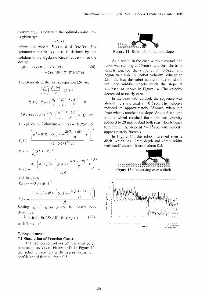
Figure l2: Robot climbing up a slope

As a result, in the case without control, therobot was running at 55mm/s, and then the frontwheels touched the slope at t = 0.5sec. andbegan to climb up. Robot velocity reduced to25mm/s. But the robot can continue to climbuntil the middle wheels touch the slope atl :9sec. as shown in F igure 14. The veloc i tydecreased to nearly zero.

In the case with control, the sequence wasalmost the same until / - 0.5sec. The velocityreduced to approximately 35mm/s when thefront wheels touched the slope. At t = 6 sec., themiddle wheel touched the slope and velocityreduced to 28 mm/s. And both rear wheels beginto climb up the slope at t =15sec. with velocityapproximately 2Omm/s.

In Figurc 13, the robot traversed over aditch, which has 32mm depth and 73mm widthwith coefficient of friction about 0.5.

Figure l3 :

This g

N , r r ) , N , r , { r - 1 4 1 ' r L " ' 1 ol r '

\ 1 , K )

ives the following solution with plry > 0:

Iri * o,'^,[n. ,,,, * 2(Q, '(t,)R)' '

"),) '

2 (Q , , ( v )R ) ' t

) ) ' '

F, '))

2P,.(v) + P. .(v'(+ -(+)' +l = Q..(v)

4 , ( " ) =19,,0)R) ' '

F,

4. . (u) - | {Q, ,o) i l

and the gains

K,(v) = (0, , (u)n ' ) '

Setting ,ri =,

dynamics:

f,/ K, (v) gives the closed loop

i - ( ;1r,) + B(v)rK(v)) i + W (v)e,,(x2)

with i =,x -,x-

7. Experiment7.1 Simulation of Traction Control

The traction control system was verified bysimulation on Visual Nastran 4D. In Figure 12,the robot climbs up a 30-degree slope withcoefflcient of friction about 0.5.

(21)

56

0 3

9 o 6

. , j f lE . o o | '. s t ]F l i

: , , F Lu l ;'

; ''i;,

Thammasat Int. J. Sc. Tech.. Vol. 10. No. 4. October-December 2005

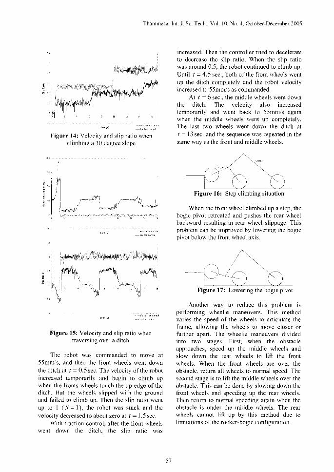
increased. Then the controller tried to decelerateto decrease the slip ratio. When the slip ratiowas around 0.5, the robot continued to climb up.Until / : 4.5 sec., both of the front wheels wentup the ditch completely and the robot velocityincreased to 55mm/s as commanded.

At t = 6 sec.. the middle wheels went downthe ditch. The velocity also increasedtemporarily and went back to 55mm/s againwhen the middle wheels went up completely.The last two wheels went down the ditch atI = l3 sec. and the sequence was repeated in thesame way as the front and middle wheels.

Figure 16: Step climbing situation

When the front wheel climbed up a step, thebogie pivot retreated and pushes the rear wheelbackward resulting in rear wheel slippage. Thisproblem can be improved by lowering the bogieoivot below the front wheel axis.

Figure l7: Lowering the bogie pivot

Another way to reduce this problem isperforming wheelie maneuvers. This methodvaries the speed of the wheels to articulate theframe, allowing the wheels to move closer orfurther apart. The wheelie maneuvers dividedinto two stages. First, when the obstacleapproaches, speed up the middle wheels andslow down the rear wheels to lift the frontwheels. When the front wheels are over theobstacle, retum all wheels to normal speed. Thesecond stage is to lift the middle wheels over theobstacle. This can be done by slowing down thefront wheels and speeding up the rear wheels.Then return to normal speeding again when theobstacle is under the middle wheels. The rearwheels cannot lift up by this method due tolimitations of the rocker-bogie configuration.

I i,.,hs['r'foi\ Jl:,'',J,

rlli,fti,tii ;il

Figure l4: Velocity and slip ratio whenclimbing a 30 degree slope

\itor,",u,"q v" r**"/'.1

,J .^lnt ''l***"/[

444&\,1"/ tu/flllP

Figure 15: Velocity and slip ratio whentraversing over a ditch

The robot was commanded to move at55mm/s. and then the front wheels went downthe ditch at / = 0.5sec. The velocity of the robotincreased temporarily and begin to climb upwhen the fronts wheels touch the up-edge of theditch. But the wheels slipped with the groundand failed to climb up. Then the slip ratio wentup to I ( S - I ), the robot was stuck and thevelocity decreased to about zero aI I : 1.5 sec.

With traction control, after the front wheelswent down the ditch. the slio ratio was

Figure | 7:

5'7

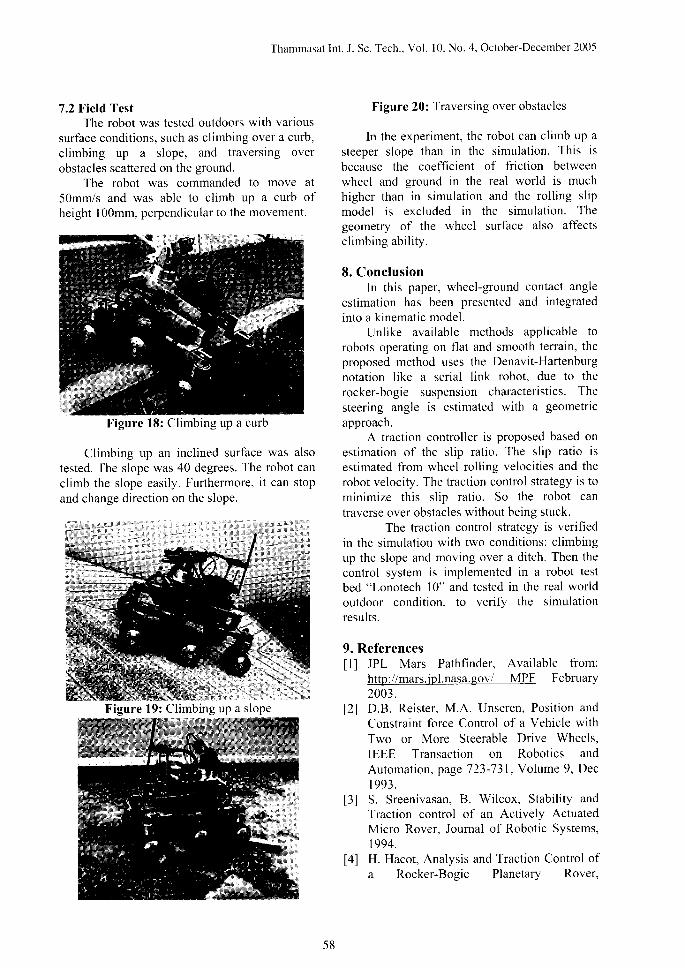
7.2 Field TestThe robot was tested outdoors with various

surface conditions, such as climbing over a curb,climbing up a slope, and traversing overobstacles scattered on the ground.

The robot was commanded to move at50mm/s and was able to climb up a curb ofheight l00mm, perpendicular to the movement.

Figure 18: Climbing up a curb

Climbing up an inclined surface was alsotested. The slope was 40 degrees. The robot canclimb the slope easily. Furthermore, it can stopand change direction on the slope.

Thammasat Int. J. Sc. Tech., Vol. 10. No. 4, October-December 2005

Figure 20: Traversing over obstacles

In the experiment, the robot can climb up asteeper slope than in the simulation. This isbecause the coefficient of friction betweenwheel and ground in the real world is muchhigher than in simulation and the rolling slipmodel is excluded in the simulation. Thegeometry of the wheel surface also affectsclimbing abil ity.

8. ConclusionIn this paper, wheel-ground contact angle

estimation has been presented and integratedinto a kinematic model.

Unlike available methods applicable torobots operating on flat and smooth terrain, theproposed method uses the Denavit-Hartenburgnotation like a serial link robot, due to therocker-bogie suspension characteristics. Thesteering angle is estimated with a geometricapproach.

A traction controller is proposed based onestimation of the slip ratio. The slip ratio isestimated from wheel rolling velocities and therobot velocity. The traction control strategy is tominimize this slip ratio. So the robot cantraverse over obstacles without being stuck.

The traction control strategy is verifiedin the simulation with two conditions: climbingup the slope and moving over a ditch. Then thecontrol system is implemented in a robot testbed "Lonotech 10" and tested in the real worldoutdoor condition, to verify the simulationresults.

9. References

[1] JPL Mars Pathfinder, Available from:http://marsjpl.nasa.gov/ MPF February2003.

[2] D.B. Reister, M.A. Unseren, Position andConstraint force Control of a Vehicle withTwo or More Steerable Drive Wheels,IEEE Transaction on Robotics andAutomation, page 723-731, Volume 9, Dec1993.

t3l S. Sreenivasan, B. Wilcox, Stability andTraction control of an Actively ActuatedMicro Rover, Joumal of Robotic Systems,1994.

[4] H Hacot, Analysis and Traction Control ofa Rocker-Bogie Planetary Rover,

Figure 19: Climbing up a slope

58

t \ lI ' t

t6l

M.S.Thesis, Massachusetts Institute ofTechnology, Cambridge, MA, 1998.K. Iagnemma, S. Dubowsky, Mobile RobotRough-Terrain Control (RTC) for PlanetaryExploration, Proceedings of the 26'n ASMEBiennial Mechanisms and RoboticsConference, Sep.10-13, 2000, Baltimore,Maryland.K. Yoshida, H. Hamano, Motion Dynamicsof a Rover with Slip-Based Traction Model,

Thammasat lnt. J. Sc. Tech.. Vol. 10. No. 4. October-December 2005

Proceeding of 2002 IEEE InternationalConference on Robotics and Automation,2002.John J. Craig, Introduction to RoboticsMechanics and Control. Second Edition,Addison-Wesley Publishing, 1 989.Patrick F. Muir, Charles P. Neumann,Kinematic modeling of wheeled mobilerobots, Joumal of Robotics Systems, Vol.4,No.2, pp.281-340, 1981.

l l l

l8l

59