TR82-002

PARALLEL SOLUTION OF EIJ.JPTIC PARTIAL DIFFERENTIAL

EQUATIONS ON A TREE MACHINE

by

Roy Peredo Pargas

A dissertation submitted to the faculty of the University of North Carolina at Chapel Hill in partial fulfillment of the requirements for the degree of Doctor of Philosophy in Computer Science.

Chapel Hill

1982

Approved by:

ROY PEREDO PARGAS. Parallel Solution of Elliptic Partial Differential Equations on a Tree Machine. (Under the direction of DR. GYULA A. MAGO.)

ABSTRACT

The numerical solution of elliptic partial differential equations (pde's) can often be reduced to the solution of other relatively simple problems, such as solving tridiagonal systems of equations and low-order recurrence relations. This thesis describes elegant and efficient tree machine algorithms for solving a large class of these simpler problems, and then uses these algorithms to obtain numerical solutions of elliptic partial pde's using methods of finite differences.

The tree machine model on which this work is based contains data only in the leaf cells of a complete binary tree of processors; one leaf cell typically holds all information pertinent to one point of the rectangular mesh of points used by the method of finite differences. An algorithm is described for communication among leaf cells using shortest paths; other algorithms are exhibited that find the first n terms of the solution to several classes of recurrence expressions in O(log n) time.

The communication and recurrence expression tree algorithms are used to describe algorithms to solve (n xn) tridiagonal linear systems of equations. A number of direct methods are shown to require O(log n) time, whereas other direct methods require O((log n) 2) time. Iterative methods are shown to require O(log n) time per iteration. The asymptotic complexity of both direct and iterative methods implemented on sequential, vector, array, and tree processors are compared.

The tridiagonal linear system solvers and the communication algorithms are used to describe algorithms to solve (n 2 x n 2) block-tridiagonal linear systems iteratively. Both point iterative and block iterative methods are shown to require O(n) time per iteration. Alternating direction implicit methods req_uire O(n log n) time per iteration. The asymptotic complexity of methods implemented on sequential, vector, array, and tree processors are again compared.

m:mCATION

To Maris, Rica, and Rebecca, who made the bad times good

and the good times better.

ACKNOWLEDGEMENTS

A dissertation is never the product of one person alone. There are several people to whom I wish to express my gratitude.

I thank Dr. Gyula A. Mag6, my adviser, who always managed to point me in the right direction whenever I got stuck. Besides suggesting the original research topic, he provided many hours of guidance and carefully read the numerous drafts of this dissertation.

I also thank the other members of my committee, Dr. Donald F. Stanat, Dr. Bharadwaj Jayaraman, Dr. Steven M. Pizer, and Dr. Douglas G. Kelly. Don Stanat, in particular, has been a close friend as well as an adviser.

I am very grateful to all my friends, especially to Anne Presnell and Ed Jones. Anne developed the communication algorithm, Atomic Rotate Left, which proved extremely useful. Ed was always willing to listen, and helped improve many of the algorithms.

Finally. I wish to thank my family, especially my mother and parents-in-law for many years of encouragement and support.

This work was supported in part by the National Science Foundation under Grants MCS"IB-02778 and MCSB0-04206.

TABLE OF CONTENTS

Chapter 1. Introduction

Chapter 2. Preliminaries A. The Second-Order Partial Differential Equation B. The Method of Finite Differences C. The Tree Machine (TM)

1. Previous Work 2. Overview of TM 3. The Microprogramming Language 4. The Tree Cells 5. Example and Analysis of an Algorithm 5. Relationship Between TM and MM

Figures

Chapter 3. Basic Tree Algorithms A. Introduction B. Composition and Substitution

1. Overview 2. Parallel Solution of Recurrence Expressions

The Tree Machine Algorithm: LR1 Extensions

3. Quotients of Linear Recurrences Extensions

4. Second- and Higher-Order Linear Recurrences Extensions

C. Atomic Rotate Left: ROTLA D. General Data Communication Algorithm: GDCA

1. Description 2. Execution Time of K-shift

Figures

Chapter 4. Tridiagonal Linear System Solvers A. Overview B. Direct Methods

1. Traditionally Sequential Algorithms Thomas Algorithm Gaussian Elimination

2. LU Decomposition A Method Using Second-Order Linear Recurrences Recursive Doubling

3. Methods Vsing Cyclic Reduction Cyclic Reduction Euneman Algorithm

C. Iterative Methods 1. Jacobi and Jacobi Over-relaxation 2. Gauss-Seidel and Successive Over-relaxation 3. Red-black Successive Over-relaxation

page

1

5 5 5 9 9 9

11 12 14 15 18

23 23 24 24 25 29 33 34 37 38 40 41 45 45 49 55

70 70 74 74 74 75 77 79 80 82 82 84 85 85 88 89

4. Parallel Gauss: An Iterative Analogue of LU Decomposition 91 D. Summary and Conclusions 93

1. General Remarks 93 2. Comparison of the Tree Algorithms 96 3. Comparison with Sequential, Vector and Array Algorithms 98

Figures 100

Chapter 5. Block-tridiag anal Linear System Solvers A. Overview B. Point Iterative Methods

1. Jacobi 2. Extensions 3. Jacobi Over-relaxation 4. Gauss-Seidel and Successive Over-relaxation 5. Red-black Ordering of Mesh Points

C. Block Iterative Methods 1. Line Jacobi 2. Line Jacobi Over-relaxation 3. Line Gauss Seidel 4. Line Successive Over-relaxation

D. Alternating Direction Implicit Method E. Remarks F. Detailed Time Analysis of the Jacobi Method Figures

Chapter 6. Conclusion Suggestions for Further Work

References

111 111 113 114 117 120 121 124 126 126 128 129 131 132 135 136 139

154 157

159

LIST OF F1GURES

Figure

2.1 A (7x9) rectangular mesh used in the method of finite differences.

2.5 A (35x35) block-tridiagonal coefficient matrix.

2.2 Basic structure of the tree machine TM.

2.4 Sample statements of the microprogramming language.

2.5 L, T, and C cells.

2.6 Control programs for L, T, and C cells.

2.7 Sample L, T, and C cell microprograms.

2.8 Analysis of a tree algorithm.

3.1 Initial and final contents of n=B L cells executing LRl.

3.2 A composition step during execution of LRl.

3.3 A substitution step during execution of LRl.

3.4 Values communicated during the composition sweep of LRl.

3.5 Values communicated during the downward sweep of LRl.

3.6 Analysis of LRl.

3.7 Upward and downward sweeps of LRl for n=5 on an 8 L cell tree machine.

3.6 Analysis of FRACTJON.

3.9 Composition and substitution during execution of LR2.

3.10 Analysis of LR2.

3.11 One implementation of ROTL.

3.12 ROTLA upward sweep.

3.13 ROTLA downward svreep.

3.14 Analysis of ROTLA

3.15 Examples of data communication among the L cells.

3.16a GDCA initialization upward sweep.

3.16b GDCA initialization downward sweep.

3.17 Algorithm constructing the T cell directories for GDCA.

3.18 Analysis of GDCA directory construction.

3.19 Examples of the movement of data during execution of GDCA.

3.20 K-sbift simulation results for N = 16 1 cells.

3.21 K-shift simulation results for N = 32 1 cells.

3.22 K-sbift simulation results for N = 64 1 cells.

4.1 Analysis of the Thomas algorithm.

4.2 Analysis of Gaussian elimination.

4.3 Analysis of 1U decomposition.

4.4a Analysis of a variant of 1U decomposition.

4.4b Recursive doubling for n=B.

4.4c Analysis of a variant of recursive doubling.

4.5 Data communication in cyclic reduction.

4.6 1 cell sequence numbers and mask used in cyclic reduction.

4. 7 Communication among the 1 cells during cyclic reduction.

4.8 Analysis of cyclic reduction.

4.9 Analysis of the Buneman algorithm.

4.10 Analysis of the Jacobi method.

4.11 Analysis of the Jacobi over-relaxation method.

4.12 Analysis of the Gauss-Seidel method.

4.13 Analysis of successive over-relaxation.

4.14 Analysis of red-black successive over-relaxation.

4.15 Analysis of red-black parallel Gauss.

4.16 Solving two tridiagonal linear systems simultaneously.

4.17 Summary of analyses of direct tridiagonal linear system solvers.

4.16 Summary of analyses of iterative tridiagonal linear system solvers.

4.19 Comparison of the complexity of direct tridiagonal linear system solvers implemented on sequential, vector, array, and tree processors.

4.20 Comparison of the complexity of iterative tridiagonal linear system solvers implemented on sequential, vector, and tree processors.

5.1 A (7x9) rectangular mesh-used by the method of finite differences.

5.2 A (35x35) block-tridiagonal coefficient matrix.

5.3 Initial layout of the mesh points among the L cells.

5.4 Analysis of one iteration of the point iterative Jacobi method.

5.5 Analysis of one iteration of the point iterative Jacobi over-relaxation method.

5.6 Snapshot midway through one iteration of the sequential Gauss-Seidel algorithm.

5. 7 Snapshots during the startup period of the parallel Gauss-Seidel algorithm.

5.8 Analysis of one iteration of point iterative Gauss-Seidel.

5.9 Analysis of one iteration of point iterative successive over-relaxation.

5.10 Checkerboard pattern used in red-black successive over-relaxation.

5.11 Analysis of one iteration of the line Jacobi method.

5.12 Analysis of one iteration of the line Jacobi over-relaxation method.

5.13 Block-iterative wave snapshots during the startup period of the line Gauss-Seidel algorithm.

5.14 Analysis of one iteration of the line Gauss-Seidel algorithm.

5.15 Analysis of one iteration of the line successive over-relaxation algorithm.

5.16 Analysis of one iteration of the alternating direction implicit method.

5.17 Rates of convergence of several iterative methods.

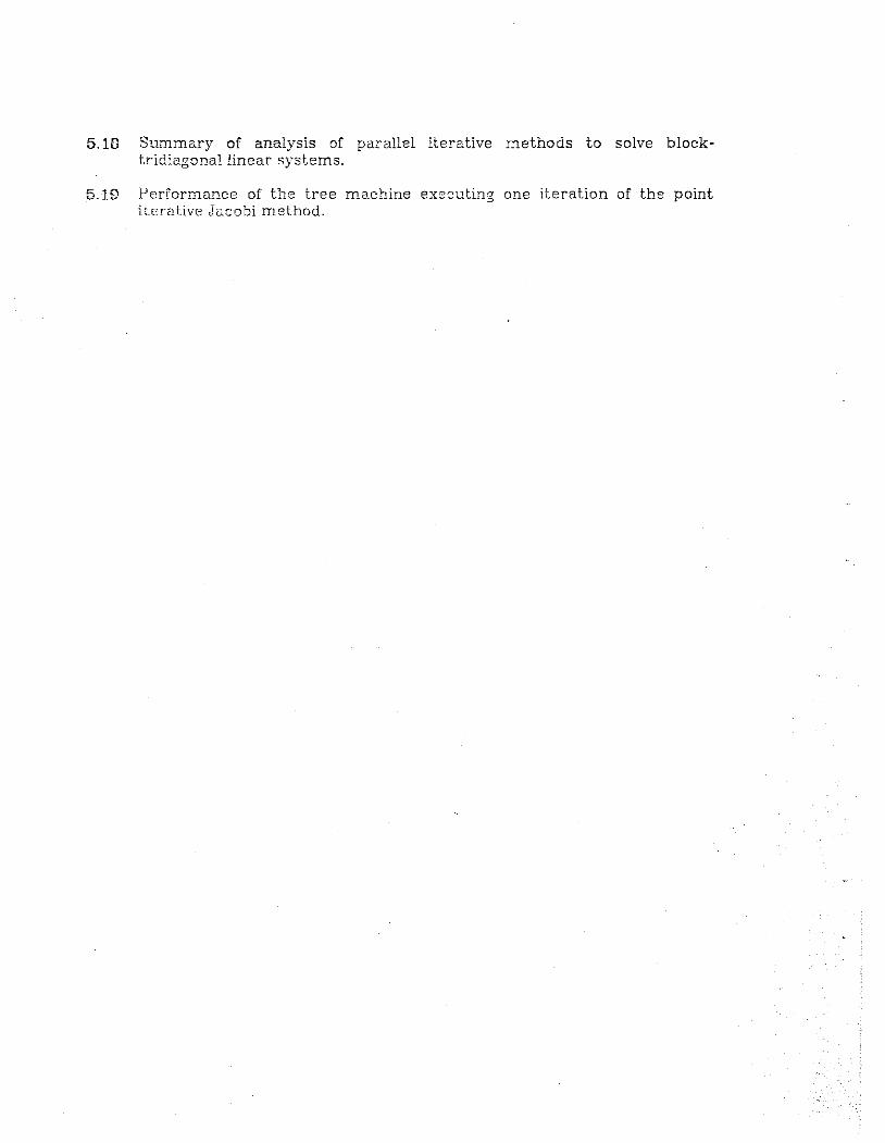
5.10 Summary of analysis of parallel iterative methods to solve block­tridiagonallinear systems.

5.19 Performance of the tree machine executing one iteration of the point itcrntive Jc.cobi method.

CHAPTER 1. INTRODUCTION

The formulation of mathematical models in engineering and the physical

sciences often involves partial differential equations (pde's). Rice et o:l. [Rice79]

give as examples models to perform

nt:.merical weather prediction ... , the simulation of nuclear reactors and fusion reactors, the analysis of the structural properties of aircraft and bridges, the simulation of blood flow in the human body, the computation of air flow about an aircraft or aerospace ve:t-Jcle, the propagation of noise through the atmosphere, and the simulation of petroleum reservoirs.

The numerical solution of partial differential equations often reduces to a prob-

!em of solving very large linear systems of equations in which the coefficient

matrix is sparse and of a special structure (e.g. tridiagonal, block-tridiagonal).

The sheer number of operations required (some applications are estimated to

require at least 1018 operations, or about 107 hours on a CDC STAR-100) has

motivated the search for faster methods of computing.

During the last fifteen years, much attention has been on the design and

implementation of parallel algorithms to solve pde's on array or vector proces-

sors such as the JLLJAC-JV, the CDC STAR-100, and the CRAY-1. One approach has

been to implement already existing algorithms originally intended for sequential

machines on a parallel processor. This almost always requires a modification of

the algorithm in order to introduce parallelism best suited to the machine's par-

ticular capabilities. One often hears of "vectorizing" a sequential FORTRA..'l pro-

gram in order for it to run etiicienlly on a vector processor. Another approach

has been to design new parallel algorithms specially suited for a particular

-1-

machine. At times, the algorithms produced, although efficient on a parallel

processor, are inefficient on a sequential processor1. The lesson one immedi-

at.ely learns when studying parallel algorithms is that. the requirements for

efficiency are different from those for sequential computers. One rather

difficult problem for the designer of parallel algorithms is communication

among the processing elements of a parallel machine.

The parallel processor we study in this disserta'cio,-, is a tree machine, i.e., a

network of processors (nodes, cells) interconnected to form a binary tree

[1:ag679a, TollBl, Brov:79]. ln the design proposed by Mag6, hereafter referred to

as M'.f, the nodes (of which there are two types) are small. For example, they

migbl contain a bit-serial ALU, bit-serial communication between nodes, a few

dozen registers, and a small memory to hold dynamically loaded micropro-

grams. J,JJ,f is a small-grain system with possibly several hundred thousand

nodes. (Here, granularity is defined as the size of the largest repeated element

[SuDDBl].) This is in contrast to large-grain tree machines whose nodes are von

Neumann processors, possibly numbering in the hundreds or thousands. (Sys-

tolic arrays [Kung79] are probably the best known examples of small grain sys-

terns.)

The problem we investigate in this dissertation is the implementation on a

tree machine of numerical methods to solve seconi-order elliptic partial

differential equations using finite differences. In particular, we seek to answer

three questions.

1F'o:r exaT.p:e, :recu:rs:ve do-Jb~::1g [S:o::~73a, S!.o~75] is a pa.:'a2:e2 a~go:-ithm tha: solves a?I (n xn) tr~d:e.,go:ne.2 ::..·rw;::-- ~ys:.e~ o:· eq·Je.;.jo:-:Js (a b~s:c S'.l'Sp:-o~~o:-:T. o~ pd-: so~ve:-s) :_, O(jog n) time 0:1 6..."'1. ar­ray p7"ocef!C'. 0::1 a secr..:e::1::i. p;or.;.;::;;:so.:, rec-a:-s~vc do-.1:.::~:-Jg :w.:,.;,es O(n~og n) time, compe.::ed :o O(n) ti!T~e req-J..:..rt.:d Dy Ge.:.l~s~.::.::1 e~~:T..~::la:~o:I.

-2-

( 1) Can solutions to elliptic partial differential equations be implemented

efficiently on a tree machine?

(2) How does the tree machine implementation compare with implementations

on other high performance machines, such as vector computers?

(3) What conclusions regarding tree machine programming do these implemen-

lations provide?

l\o attempt is made to design new elliptic pde solvers. All methods mentioned in

this dissertation have been designed and analyzed previously.

To answer the above questions, we present a description of a simple

abstract special-purpose tree machine and several classes of algorithms

designed to run on it. The dissertation is organized as follows.

Chapter 2. Preliminaries

• Overview of partial differential equations and the method of finite differences.

• A description of the tree machine and its component cells.

• The algorithmic language used to specify some of the algorithms.

• Analysis of algorithms.

Chapter 3. Tree mac·bine algorithms: algorithms that form the basic building blocks of tridiagonal and block-tridiagonal linear system solvers

• O(log n) algorithms that solve low-order linear recurrences and recurrence expressions. such as continued and partial fractions.

• Tree communication algorithms, that is, techniques that allow efficient communication among the leaf cells of the tree. Efficient communication among the processors is essential for an efficient implementation of paral­lel algorithms. We present algorithms that cyclically shift a vector of ele­ments stored in the leaf cells a distance k to the left or right in O(k) time if k > logn, where n is the number of leaf cells in the tree, and O(log n) other­wise.

Chapter 4. Tridiagonal linear system soh·ers: tree machine implementations of direct and iteraliYe parallel methods to solYe tridiagonal linear systems

-3-

• Direct methods include Gaussian elimination, the Thomas algorithm, LU decomposition, a method using second-order linear recurrences {similar to Slone's recursive doubling [KoSl73], [Slon75]), cyclic reduction and. the Buneman variant of cyclic reduction. On a sequential computer, all of the methods require O(n) lime. On a tree machine, cyclic reduction and the Buneman variant require O{log n) 2 time; Gaussian elimination, the Thomas algorithm, LU decomposition, and the recursi,·e doubling variant all require O(log n) time.

• Iterative methods include the Jacobi method, Jacobi over-relaxation, the Gauss-Seidel method, successive over-relaxation, red-black successive over-relaxation, and the iterative analog of LU decomposition (developed by Traub [Trau73]). All require O(n) lime on a sequential computer and O(log n) time on a tree machine per iteration.

• Comparison of results obtained with those for parallel and vector proces­sors

ChaptEr G. JleratiYe block-tridiagonallines.r £ystem solvers

• Tree machine implemenliltions of point iterative, block iterative, and alter­nating d1reclion implicit (AD!) methods to solve an {n xn) block-tridiagonal linear system. The point iterative methods studied are the Jacobi method, Jacobi over-relaxation, Gauss-Seidel, successive over-relaxation (SOR), and a \'ariant of SOR, red-black succe,ive over-relaxation. On a sequential computer, these methods require O(n 2) time per iteration. Tree machine algorithms require O(n) lime per iteration. The block iterative methods studied are block Jacobi, block Jacobi over-relaxation, block Gauss-Seidel, and block SOR; all require O(n) lime per iteration. ADJ methods studied require O(n log n) time per iteration.

• Detailed analysis of the lime required by the Jacobi method

Chapter 6. Conclusions

-4-

CHAPTER 2. PREIJMINARJES

A The Second-order Partial Differential Equation

The general second-order partial differential equation (pde) in two dimen-

sions

a2z 82z il2z Bz Bz a-2-+ b-

0 8 + c-

2-+ F(-;:;-.-

8 ,x,y) = o

OX X y oy vX y (2.1)

may be classified on the basis of the expression b 2 - 4ac as follows:

elliptic if b 2 - 4ac < 0

parabolic if b 2 - 4 ClC : 0

hyperbolic if b 2 - 4ac > 0.

Members of each class can be transformed, possibly with a change of variables,

into a canonical form:

elliptic

parabolic (2.2)

hyperbolic = G

-5-

where G = GU. TJ, z, az I a~. 8z/ {JTJ). This dissertation deals exclusively with

elliptic equations, of which the most commonly studied ones are Laplace's equa-

tion (2.3) and Poisson's equation (2.4).

a2z --= constant. ayz

(2.3)

(2.4)

Jn this dissertation, we will investigate how one may solve problems involving

these equations on a tree machine.

B. The Method of Finite Ditl'erences

Problems involving second-order elliptic pde's are equilibrium problems.

Given a region R, bounded by a curve Con which the function z is defined (the

boundary conditions), and given that z satisfies Laplace's or Poisson's equation

in R, the objective is to determine the value of z at any point in R. The method

of finite differences is a widely used numerical method for solving this problem.

The basic strategy is to approximate the differential equation by a difference

equation and to solve the difference equation.

Consider Laplace's equation (2.3). Let R be a rectangular region and C its

perimeter. Laying a rectangular mesh with n rows, m columns, and equal spac-

ing h on the region (Figure 2.1), we want an approximation of the function z at

the interior mesh points. Once this is determined, approximations at other

points in the region may he obtained through interpolation.

-6-

One approximation is to replace the second derivatives in (2.3) with the

centered second differences, so that for z = z,,

(2.5)

and

(2.6)

Laplace's equation is therefore approximated by

(2.7)

which gives

(2.8)

illdicating that one way to represent each point z, is by a linear equation. The

object is to solve the ith equation for Z;. This method, sometimes called the

direct method. uses equation (2.8) and transforms the problem of approximating

the z values at the (n-2)(m-2) interior points to one of solving (n-2)(m-2)

linear equations in as many unknowns. The coefficient matrix of this linear sys-

tern is block-tridiagonal in structure. The example of Figure 2.1 would have a

coefficient matrix as shown in Figure 2.2.

Equation (2.8) may also be expressed as

Z; "' (z,_, + Zi+l + Z.-m + Z.tm )/4 (2.9)

suggesting that, if we know {or can approximate) the values of an interior point's

four closest neighbors, we may iteratively improve the value at the point by

replacing it with the average of its four closest neighbors. This is called the

-7-

iterative method. After assigning an initial value to each of the interior mesh

points, the method iteratively improves the approximation by replacing each

point with a weighted average of its four closest neighbors, as specified in equa­

tion {2.9). One pass through the mesh points constitutes one iteration. We may

iterate as many times as desired, until some criterion for convergence has been

satisfied. This method has been shown to have O(h 2} convergence where h is the

distance between two neighboring mesh points [Ames77].

The iterative approach involves a simple computation, in the simplest case

nothing more than the averaging of four values. Higher-order approximations of

Laplace's equation require using more points in the approximation but the basic

operation remains the taking of weighted averages. Moreover, there is a great

amount of parallel activity possible: theoretically, we may compute the ith

approximation of all interior mesh points simultaneously. On a parallel proces­

sor, it may be possible to perform one iteration (modify all points) in as little

time as it takes to modify one point. While this operation would appear to be

trivial on the JLLJAC-JV whose processing elements are interconnected to form a

rectangular mesh, the solution on a tree machine is far from obvious.

1\"e will investigate lhe implementation of iterative methods of solving

block-tridiagonal linear systems on a tree machine. (A more detailed discussion

of the method of finite differences applied to elliptic pde's is given by Forsythe

and \\"asow [Fo\\"a50] and Ames [Ames77].)

-6-

C. The Tree Machine (TM) 1. Previous Work

Mag6 [Mag679a), [Mag6BO] has proposed a cellular computer, here referred

to as MM, organized as a binary tree of processors, that allows simultaneous

evaluation of expressions stored in the leaf cells of the tree. It directly executes

functional programming languages, a class of languages developed by Backus

[Back7B], in which the expression of parallelism is natural. Tolle [TollBl) has

proposed a similar tree-structured cellular computer with more powerful. but

more complex, cells. In both designs, processors contained in the tree cells are

capable of independent operation, thus providing the potential for parallel com-

putation. Williams [WillBl] studied parallel associative searching algorithms and

presented several techniques to predict and analyze the amount of time and

storage required by the algorithms if run on JJJJ. Koster [Kost 77] and Mag6,

Stanat, and Koster [MaSKBl] developed a method for obtaining upper and lower

bounds of the execution lime of programs run on MM. Their analysis carefully

accounts for communication and storage management costs. Parallel algo-

rithms for tree machines have also been developed by Browning [Brow79] for a

variety of applications, including sorting, matrix multiplication, and the color

cost problem, and by Bentley and Kung [BeKu79] for searching problems.

Leiserson [Leis78] studied systolic trees and how to maintain a priority queue on

one.

2. Over-vie\'/ of 'I'M

In this section, we describe TJ.!, a special-purpose tree network of proces-

sors similar to, but of a much simpler structure and less powerful than, the

-9-

general-purpose machines proposed by Mag6 and Tolle. TM is a binary tree net­

work of processing elements in which the branches are two-way communica-tion

links (Figure 2.3). Leaf and nonleaf processing elements are called 1 cells and T

cells respectively. Attached to the root cell, functioning as the root cell's

father, is a cell called Control (C cell).

When describing algorithms, cells are sometimes referred to by their level

in the tree. The 1 cells are on level 0, the lowest leYel T cells are on level 1, the

root T cell is on level log N, and the C cell is on level log N + 1, where N is the

number of 1 cells in the tree. Two-way communication among the cells is con­

ducted through the tree branches; aT cell may communicate with its father and

two sons and an 1 cell may communicate with ils father; a C cell communicates

with lbe root T cell and with external storage, as explained below. An 1 cell may

communicate with another 1 cell by sending information up the tree through the

sending 1 cell's ancestor T cells and then back down again to the receiving 1

cell.

Jn principle, all cells operate asynchronously. However, the algorithms

presented can be more easily understood if we view the operation as proceeding

in synchronous up"·ard and downward sweeps. 1\'e note, however, that this syn­

chrony is not a necessary feature of T/.!.

An example of a task requiring a downward sweep is that of broadcasting

information to all L cells. The C cell sends information to its son the root cell,

which sends the information lo its two sons, which send the information to their

sons, and so on, until the information is simultaneously received by the 1 cells.

An example of a task requirin;; an upward sv;ecp is that of adding the values

-10-

stored in the L cells with the C cell receiving the sum.

3. The Microprogramming Language

As Hoare observed [Hoar7B], a programming language for a machine with

multiple, independent, asynchronous processing units must contain special

statements not ordinarily found in languages for sequential computers. This is,

in part, because the processing units must have a way of communicating and

·synchronizing with each other. The language he describes for multiple proces­

sors, CSP, includes statements such as parallel commands specifying possible

concurrent execution of its components, and input and output commands used

for communication between processors. Browning and Seitz [BrSeBl] concur

with Hoare and have written a compiler for Tl>!PL, a language similar to Hoare's

CSP, for the purpose of implementing algorithms on a tree machine. Programs

presented in this diSEcrtation will be written in an algorithmic language whose

special features are described brietl.y below. Communication between tree cells

will be handled by SE'\D and RECEI\'E commands. The CASE command and the

concurrent execution of statements are also explained. Figure 2.4 shows a few

sample statements.

SJ::!\D and RECEIVE require cooperation between two cells. In order for a

cell to execute a SE'\D statement, the receiving cell must execute a RECEIVJ::

statement (Figures 2.4a and 2.4b). It may happen that a cell wishing to send

(receive) data must wait until ils partner is ready. A CASE statement allows a

cell to waiL for more than one other cell. Figure 2.4c shows a cell attempting to

receive data from its left s'm (cas" c.l), receive data from its right son if n is

-11-

currently nonzero (case c.2). or send data to its father if n is nonnegative (case

c.3). Only one of the cases v.ill be executed and the choice may depend upon the

value of n. If for example, n is currently 0, only cases c.l and c.3 may be exe­

cuted. If both the cell's left son and father are ready to communicate, the cell

randomly chooses between them, executes the statement, and either incre­

ments n (left son was chosen) or sets n lo 0 (father was chosen). If neither

father nor left son is ready to communicate, the cell waits until one is ready. We

allow only one SEJ\D or RECEIVE statement for each condition of a case state­

ment. Figure 2.4d shows concurrent execution. Data must be sent to both sons

but the order of execution is not important; the first ready son is sent the data

first. Ead the statement been written

L.SEI\D(X); R.SEI\D(Y);

the right son may be unnecessarily delayed from recei\ing its data if the left son

is not ready to execute an F.RECEJVE statement.

4. The Tree Cells

A cell (L, T, or C) consists of a small memory and a processor (Figure 2.5).

The memory holds the control program, a single cell microprogram, and a small

number of registers used to store date. At all times, a cell processor is under

the exclusive control of either the control program or the cell microprogram.

The control programs are shown in Figure 2.6.

The L cell control pro::;ram (Figure 2.Ba) instructs the processor to wait

until a micropco::;ram set, consisting of a T cell and an L cell microprogram,

- 12-

arrives. When one does, the control program instructs the processor to save the

L cell microprogram and then to execute the microprogram, i.e., control o[ the

processor is transferred to the microprogram. The microprogram specifies ( 1)

how much data to read, (2) in which variables to store the data, (3) how to pro­

cess the data, and (4) what to send back to the father. The microprogram

retains control of the processor until its execution is complete. At that time,

control of the processor returns to the control program. Note that while the

control program is executing, the L cell expecti', and should only receive, a

microprogram sel. While the microprogram is executing, the L cell may only

receive data.

The T cell control program (Figure 2.6b) instructs the processor to wail

until a microprogram set arrives. When one does, the processor sends a copy to

each of ils sons \\bile saving the T cell microprogram. It then begins executing

its microprogram. Like the L cell, control of the T cell processor returns to the

control program only after the microprogram is executed.

The C cell control program instructs the C cell processor to fetch the next

set of L, T, and C cell microprograms from external storage. The processor then

sa,·es the C ceii microprograr.1 and sends the L and T cell microprograms (the

microprogram set) to the root. T cell. The C cell then executes its micropro­

gram. After execution, control returns to the control program which proceeds

to felch the next set of microprograms from external storage.

A C cell, a T cell, and an L cell microprogram, taken collectively, may be

viewed as a global operation to be performed by all of the cells of the machine

operating in ba:-rr2ony, ,~·hereas a microprograrr1 specifies the local operation

- 13-

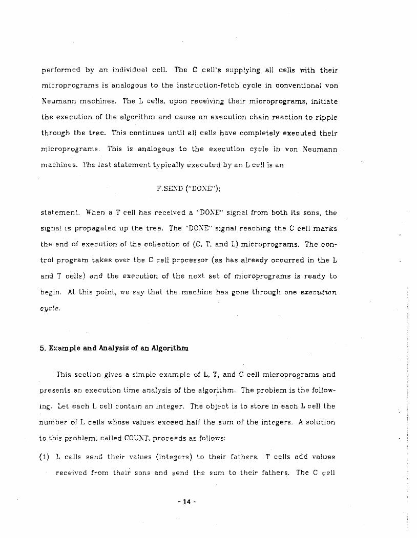
performed by an individual cell. The C cell's supplying all cells with their

microprograms is analogous to the instruction-fetch cycle in conventional von

Neumann machines. The L cells, upon recei,ing their microprograms, initiate

the execution of the algorithm and cause an execution chain reaction to ripple

through the tree. This continues until all cells have completely executed their

microprograms. This is analogous to the execution cycle in von Neumann

machines. The last statement typically executed by an L cell is an

F.SEJ\D ("DOXE");

statement. When a T cell has received a "DOJ\E" signal from both its sons, the

signal is propagated up the tree. The "DOXE" signal reaching the C cell marks

the end of execution of the collection of (C, T, and L) microprograms. The con­

trol program takes over the C cell processor (as has already occurred in the L

and T cells) and the execution of the next set of microprograms is ready to

begin. At this point, we say that the machine has gone through one executwn

cycle.

5. Example and Analysis of an Algorithm

This section gives a simple example of 1, T, and C cell microprograms and

presents an execution lime analysis of the algorithm. The problem is the follow­

ing. Let each L cell contain an integer. The object is to store in each L cell the

number of L cells whose values exceed half the sum of the integers. A solution

to this problem, called COul\T, proceeds as follo11·s:

(1) L cells send their values (integers) to their fathers. T cells add values

received from their sons and send the sum to their fathers. The C cell

- 14-

receives the sum and sends it back down through tree to the L cells.

(2) Each 1 cell compares its value with the sum and sends up a "1" if its value

exceeds half the sum. Otherwise it sends up a "0". The T cells add the

values received from their sons and send the sum to their fathers. The C

cell returns the value it receives through the tree to the L cells.

The L, T, and C cell microprograms are shown in Figures 2. 7a-c.

Each algorithm presented in this dissertation will be followed by a time

analysis. For simplicity, we assume that cells en each level of the tree (the 1

cells are on level 0, their father T cells are on level 1, and so on) operate syn­

chronously. The design of the algorithms make this a reasonable assumption.

We emphasize, however, that this is not an essential feature of either TM or MM.

The analysis will be expressed as the number of parallel arithmetic operations

(additions and multiplications) and the amount of communication time required.

If all of the L cells must execute a multiplication, for example, we assume that

all of the 1 cells take the same amount of time to do it. Their collective action is

considered, therefore, as a single multiplication. Communication is measured in

steps where one step is defined as the time required for one cell to send one unit

of information (one number, one character) to an adjacent cell. A cell may

simultaneously send and receive information from cells adjacent to it. A T cell

may therefore send as many as three numbers to its father and sons and receive

three numbers from its father and sons in one time unit or step. The analysis of

the COl::\T algorithm is shown in Figure 2.8.

-15-

6. Relationship between TM and MM TM is a model of a tree machine. Its primary function is to serve as a vehi-

cle for describing tree machine algorithms. We may implement the algorithms

described in this dissertation by incorporating TM into MM. a general-purpose

machine capable of executing programs wrilten in an FFP language. MM. during

a process called partitioning (Mag679a], identifies the innermost applications of

an FFP expression and, for each, constructs a binary subtree among the T cells.

During subsequent machine cycles, these component trees machines simultane-

ously reduce the innermost applications. After reduction, the new innermost

applications are identified and the process is repeated. Each of these com-

ponent tree machines may be considered an instance of TM.

The embedding of TU into MM would be fairly straightforward. There are

only a few details that need to be explicitly stated. First, all of the algorithms

described on TM require that the processors contained in the T cells be able to

execute slightly more complex programs than are described by Mag6. More-

over, T cells in TM are supplied user-defined microprograms (in MM. only the L

cells receive microprograms, T cell programs are built-in). In short, aT cell pro-

cesser should hose the processing power of an L cell processor. Since all T

nodes execute the same microprogram, such capability would be easy to add to

the design described by Mag6 [Mag679a].

Secondly, the comp,ment tree machines formed in UM after partitioning

are seldom complete binary trees. All of the algorithms described on TM, there-

fore, should execute correctly on incomplete, as well as complete, binary trees.

Care was taken to ensure that this, in fact, be the case.

-16-

Finally, there is the question of interrupts. In MM. the root T cell periodi­

cally issues an interrupt to perform storage management. This interrupt causes

all component tree machines still in the reduction process to temporarily halt

their operations. Storage management may move the contents of the L cells of

some component tree machines. If so, these component tree machines must be

rebuilt (i.e., the branches between the L cells and the T cells must be redefined)

and any information stored in the T cells of these machines before the interrupt

must be reconstructed. It is necessary, therefore, that TM algorithms be able to

perform this reconstruction easily. Again, care was taken to ensure this fact.

Alternatively, it would be possible to have MM mark certain component tree

machines as ''uninterruptible" (this would require a minor modification of the

machine d<escnbed by Mag6 [Mag679e.]). The machine would then delay storage

management until the specially marked tree machines had completely reduced

their applications.

Eowever, the problem of interrupts may be moot if an elliptic pde is to be

solved. Such problems usually deal with a great many data. It is likely that the

entire machine, 1JM, would be dedicated to this purpose. If so, then the elliptic

pde solver could be allowed to execute uninterrupted.

-17-

z ----- z 1---- ~------- 9------- e------ e------ e------- e------ ze I o I Zg • • • • o zl7 I R I • • ii-m • • • •

C-> jh

• • 0 Zi-1-- Z·--- Zi+l • • • I ' I • • • • Zi+m • • • • z.s • • • • • • Zs2 Z5s

y i I Z54 ____ ------- ----- a-------- a-------- a------- ~~~------- Ze1---- z62

X

Figure 2.1 A rectangular mesh with n=? rows and m=9 columns. The mesh points are labeled Zc through Z52 in row major order. Each interior poir.t Z; (that is, eact point not or. the perir:"Jeter Cj has as its four dosest r.eighbors the points Z;-m· Zi-Io Zi+1• and Zi+m· l\otethat tlce carne" pointsZ(;, Zs, Zs4. and Z52 do not have any interior pcints as neigtbors and will not participate directly in ar:y compt:tatior:. They are included to make the subscripting of points regular.

-4 1 1 J

_, J 1 J -4 J J

J -4 J J 1 _, J J

J -4 J J

0 J 4 1 J .

" 1 J J -4 1 J

J 1 -4 1 J J J -4 ' 1

1 J -4 J J J J -4 J J

J J -4 J l -- J J

J 1 -4 1 J 1 J -4 J J

1 J -4 1 1 J 1 -4 J 1

1 J -4 1 1 J J _,

l

' -4 1 1 1 1 -4 I J

J 1 -4 1 1 1 J -4 J 1

1 1 -4 J J 1 1 _, 1 J

0 l l -4 1 l -4 J

l J _, 1 1 1

_, 1 1 1 -4 1

1 1 _, 1 J 1 _,

1 J 1 -4

Figure 2.2 The coefiicier_t matrix of the system of linear equations resulting from the example of Figure 2.1 is (35x35) and block-tridiagonal in structure. Each of the diagonal blocks is tridiagonal; each of the of-diagonal blocks is diagonal. The r::umber of block equalior.s is n-2=5 and the order of each block is m-2=7, where n ar.d mare the :r..e.rnber of rows and coh...:.r:u~s. respectively, of the origir:al rectangular mesh.

-18-

Figure 2.3 Basic structure of the tree machine. The top node is called the C cell, interior nodes are called 1 cells, and the leaf nodes are called L cells.

(a) comment Send contents of X andY to right son. R.send(X,Y);

(b) comment Receive information from father and store in Y and Z. F.receive(Y,Z);

(c) comment Case statement. Communicate with first available cell. begin (c.l) case L.receive(X): (c.2) case n?'O & R.receive(Y): (c.3) case n~O & F.send(Z): end:

n:=n+l n:=n-1 n:=O

(d) comment Concurrent execution. Send contents of X andY to sons. L.send(X), R.send(Y);

Figure 2.4 Sar:1ple staterner:ts.

-19-

FATHER FATHER

u:n SON (•)

JtlGHl' SON (h)

B.OO'l' T CEU. (')

Figure 2.5 A cell (L. T. or C) cor.tains a processor and a memory, divided into three coi!lpartments. (a) An L cell communicates only with its father. (b) A T cell comi!lunicates with its father and both sor.s. (c) A C cell commurjcates with its son. the root T cell. and with external storage from which it obtair.s the mi­croprograms which it sends down to the T and L cells.

(a) L-COJ\'TROL: begin

end;

F.receive (microprogram set}. Pick out and store L cell microprogram in memory. Execute L cell microprogram.

(b) T-CONTROL: begin

end;

C-CONTROL: begin

end;

F.receive (microprogram set). Send microprogram to each son, while storing T cell

microprogram in memory. Execute T cell microprogram.

Fetch L. T. and C cell microprograms from external storage. Store C cell microprogram in memory. Send (microprogram set). Execute C cell microprogram.

Figure 2.6 Control programs for (a) L cells, (b) T cells, (c) C cell.

-20-

(a) L-COUNT: begin

comment L cells send up VALUE and receive SUM of values F.send (VALUE); F.receive (SUM);

comment Compare SUM with twice VALUE. Send result to father if 2*VALUE > SUM

then F.send (1) else F.send (0);

comment NVM is the number of L celts whose values exceed half their SUM F.receive {NUM);

comment Signal end of algorithm. F.send ("'DOl\E")

end;

{b) T-COUNT: begin

comment L cells sent up VALUEs, send sum to C cell L.receive (LVA1), R.receive (RVA1); F. send (LVA1 + RVAL);

comment C cell sent sum of values down, propagate to L cells F.receive {FVA1); L.send (FVAL), R.send (FVAL};

comment L cells sent up 1s and Os, send up sum to C cell L.receive (LVA1), R.receive (RVA1); F.send (LVA1 + RVAL);

comment C cell sent sum of ls and Os, propagate to L cells F.receive (FVAL); L.send (FVAL), R.send (FVAL);

comment Propagate "DONE" signal. L.receive (LSIGNA1), R.receive (RSIGKAL); if LSIG'\AL=RSlGKAL="DONE"

then F. send ("DONE") else F.send ("ERROR")

end:

(c) C-COUKT: begin

end;

comment Receive and return the sum of VALUEs receive (SC~l): send (St.:M):

comment Receive and return the NFM of selected L cells receive (SUM): send {Sl:M):

comment Receive "DOJ'\E" signal. F.receive (SIGNAL): if SIGNAL;< "DO!\E" then ERROR

Figure 2.7 L, T, and C cell microprograms for exar:1ple algorithm.

-21-

COUNT Parallel Operations

Step Swps Comm. Time L cells T cells C cell

+ X + X + X

1 1 21ogn + 2 0 0 logn 0 0 0 2 1 2log n + 2 0 1 logn 0 0 0

Total '

2 I 41ogn + 4 0 1 I 2Jogn I 0 0 0

Figure 2.8 Ar:alysis of the COCl\T program of Figure 2.7. Step (1) requires each cell to ser:d or:e r:Lr.Jber to Hs father d1.:ri:r..g the t:pv.rard sweep a:r3.d each cell to send one m . .:.~ber to its son(~) dt.:.riz:g the dow:r:v.--ard sweep. The total commt:.ni­calion lime frcr.:~ L cells to C cell and back is 2{logn + 1) un1ls or steps. Durir:g U:e t.:pward s·weep, each T cell must perform one addition. As there are logn lev­els cf T cells, there are a tala! of logn parallel additions performed. Step (2) is ar-alyzed similarly. Note that a sequential algorilhr.:~ wot:ld have req1.>ired 2n ad· ditior:s, 1 division, and 2n array referer..ces {to be co:c.1pared witt the number of commt:.nicatior: steps in the tree machir:e aJgorittrn).

-12-

CHAPTER 3. Basic Tree Algorithms

A. Introduction

The solution of tridiagonal and block-tridiagonal linear systems can be

decomposed into problems of solving low-order recurrence expressions. On a

tree machine. such tridiagonal and block-tridiagonal system solvers require the

L cells to communicate in certain special patterns. The purpose of this chapter

is to present the tree machine solutions to these recurrence and communica­

tion problems. The resulting algorithms form the basic building blocks of the

algorithms presented in Chapters 4 and 5.

In Section B. we present a general method for obtaining the first n terms of

recurrence expressions on tree machines in O(log n) time. Section C presents

ROTL.<\, an O(log n) communication algorithm developed by n.A. Presnell. ROTL.<\

efficiently executes the FFP primitive ROTL [Back7B] when applied to a vector of

atomic elements on a tree machine. Section D presents a general communica­

tion technique, GDCA, which allows the L cells to communicate efficiently in a

varied number of patterns. The communication time for GDCA depends on the

patlern: whenever possible, the time is less than linear in the number of L cells

participating. Both ROTLA and GDCA have been presented in a previous paper

[PrPaBl].

-23-

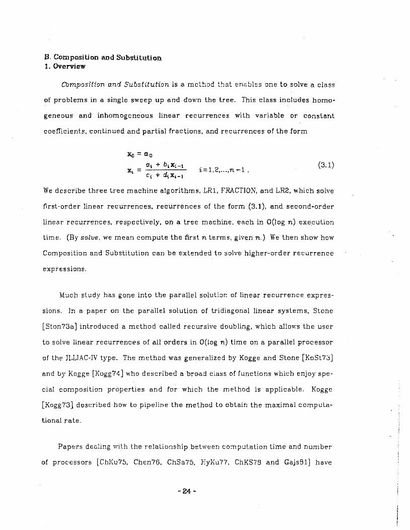
B. Composition and Substitution 1. Overview

Composition and Substitution is a method that enables one to solve a class

of problems in a single sweep up and down the tree. This class includes homo-

geneous and inhomogeneous linear recurrences with variable or constant

coefficients, continued and partial fractions, and recurrences of the form

Xc = ao

ai + bixi-t x..=

C; + ri;X;-1 i=l.2, ... ,n-1.

(3.1)

We describe three tree machine algorithms, LRl, FRACTJON, and LR2, which solve

first-order linear recurrences, recurrences of the form (3.1), and second-order

linear recurrences, respectively, on a tree machine, each in O(log n) execution

time. (By solve, we mean compute the first n terms, given n.) We then show how

Composition and Substitution can be extended to solve higher-order recurrence

expressions.

Much study has gone into the parallel solution of linear recurrence expres-

sions. In a paper on the parallel solution of tridiagonal linear systems, Stone

[Ston73a] introduced a method called recursive doubling, which allows the user

to solve linear recurrences of all orders in O(log n) time on a parallel processor

of the JLLJAC-JV type. The method was generalized by Kogge and Stone [KoSt73]

and by Kogge [Kogg74] who described a broad class of functions which enjoy spe-

cia! composition properties and for which the method is applicable. Kogge

[Kogg73] described how to pipeline the method to obtain the maximal computa-

tiona! rate.

Papers dealing with the relationship between computation time and number

of processors [ChKu75, Chen76, ChSa75, HyKu77, ChKS78 and GajsBl] have

-24-

presented bounds on the number of processors required to minimize the time to

solve first-order linear recurrences and bounds on the time required to solve the

problem given a fixed number of processors. Except for the algorithm described

by Gajski [GajsBl], the algorithms were designed for an idealized p-processor

machine on which there is no contention for memory (to obtain either instruc-

tions or data), any number of processors and memories may be used at any

lime, and communication among processors involves no delay. Hyafil and Kung

[HyKu77] established that, even with an idealized parallel processor, the best

speedup 1 one may obtain when solving first-order linear recurrences is

(2/3)p + 1/3. ln a related work [Kung76], Kung established that "many non-

linear recurrences can be sped up by at most a constant factor, no matter how

many processors are used."

Two general approaches to the problem have emerged: one approach reord-

ers the arithmetic operations required to solve the linear recurrence and distri-

butes. them among the available processors in order to minimize computation

lime [ChKu75, Chen76, ChSa75, ChKS7B]; the other uses function composition

systematically to reduce the dependencies among the variables of the linear

recurrence [Slon73a, KoSt73, Kogg73, Kogg74, GajsBl]. The algorithms

described in the next section use the latter approach.

2. Parallel So:ution of Recurrence Expressions

This section describes how properties of recurrence expressions may be

exploited to solve such expressions in parallel on a tree machine. As an exam-

pie, we present the tree machine algorithm LRJ which determines the first n

1 S?ecd-.1~ :s de5::1ed as Sp = Ttl r,. w!J.e:-e T 1 a.TJd Tp e.:;-:: -..n~ t.:::T.O'J...l-:.s of time Teq·u.ired to so]ve e. p:;o:;:c:r. 0::1 a seg'...lc::-t'~::.:: pYoccs3o:- and ap-p::-ocesso::- rr:ach,ne, respe~~ive~y.

-25-

values of a first-order linear recurrence. Some of the material presented here

was previously studied by Kogge [Kogg74] who described algorithms to solve

recurrences on an SIMD-type parallel processor.

Consider the first-order linear recurrence

(3.2)

The objective is to compute the values :x;. Q,;;i,;;n-1. To provide a uniformity

which will simplify the tree machine algorithm, we modify (3.2) by defining

(3.3)

where b 0=0 and x_ 1 is a dummy variable. Each equation of (3.2) is now a func-

tion of one variable. Next, we define X;.; to be the coefficients of the equation

expressing X; as a function of x; (i;;,.j ). i.e., if

(3.4)

Lhen

X;.1 =(a,b) (3.5)

We may no\' express (3.2) in the more general form

(3.6)

where Xu_ 1 = (a,, b.}. Equation (3.6) may be expanded as follows

-26-

x, = f (Xi.i-1• X.-1l

= I (X..<- I· I (X,-J,i-2• X.-2))

=I (Xi.i-J• I (X;-J,i-2• I (X;-2.<-3· X.-sl)) (3.7)

= =I (X;.<-J· I (X<-J.i-2• I (X<-2.<-3• ...• I (Xc.-J• X-J) ... )))

This corresponds to the nested equation

which suggests the order of operations executed by a sequential algorithm.

Eowever, we will exhibit a function g such that, for a given 1 and for all

i,j,k, -1,;;k <j <i,;;n-1.

I (X,,;. X;) = I (X,,;. I (X;.k. Xk )) = I (g (X, j. X; ,k ). X..) = I (X,,k. X..) . (3. 9)

!.:sing g. we then we show that a more efficient, parallel solution is possible. To

determine g for first-order linear recurrences, consider two linear equations

x. =a+ bx; = I(X,,;. x;)

X; = a' + b 'X.. = I (X; .k. X.. ) ·

Substituting the second equation into the first, we obtain

x, =I (Xi.j• I (Xj.k• x..))

=a+ b(a' + b'x.t)

=(a+ ba') + bb'x..

= l(g(X;,;. X;t), x..).

(3.1 D)

(3.11)

Therefore, a function g that satisfies equation (3.9) for a first-order linear

recurrence 1 is

g (X,,;. Xj.t) = X;,k =(a + ba', bb '). (3.12)

We call g a composition function because it lakes the coefficients of two equa-

lions of a recurrence expression and performs the operations required to com-

pose them. We make a few observations regarding the functions 1 and g.

-27-

Lemma 3.1

Proof

Given a recurrence expression :x, = I(Xu_ 1, :x,_ 1). Osisn-1, and a function g that satisfies equation (3.9), each variable X; can be expressed as a linear function of any x1, -1sj <isn-1. J.e., givenj<i, we can find the coefficients X;,; such that X; = I (X,,1, X;)

F'or j <i, the ( i -j }th line of equation (3. 7) gives

:x, =I (Xu-•· J (X;-I,i-2• I (X;-2.i-3• ... I (X;+I.i• x; ) ... )))

=I (g (X,,,_" g ('X;-u-2•

g (X;-2,i-3• ..• g (Xj+2.j+l• Xj+l.j ) ... ))), Xj)

= f (Xi.j• X;)

by repeated use of the property of g described by equation (3.9). "

(3.13)

Lemma3.2

Proof

lf :x, is expressed in terms of the dummy variable x_ 1 (as is Xo initially) then :x, is solved.

Equation (3.8) expresses :x, as a linear function of x_ 1• Expanding (3.8) and substituting b 0=0, we obtain

i (3.14)

=(a;+ b,a;_ 1 + · · + a 0!)b1) j;}

i.e., :x, is expressed in terms of the given coefficients b; and parameter a 0. The value of :x, is determined. 11

Lemma3.3

Proof

Let X;= I(X,,i-l• x,_ 1), Osisn-1, be a recurrence expression and g a function that satisfies

(3.15)

where Osk <j <isn-1, then, for -lsi <k <j <iSn-1,

l(g(X,,1, g(X;.ko Xk.l))) = J(g(g(X;,1. X1 . .J, Xk,l)). (3.16)

and we say that g is associati,;e under f.

From Lemma 3.1 and equation (3. 7) we can show that

(3.1 7)

Applying (3.15) twice, we obtain

-28-

:x, = t(x,.1• J(g(X1 .•• x •. t). Xj))

= 1 (g (X. .1• g (x, ·" . x • .t)). Xt) ·

Applying (3.15) twice to (3.17) in a different order, we obtain

X. = f (g (X;,J, XJ.< ), f (X<.t· Xj ))

=! (g (g (x,,,.x, . .>. x •. tl. Xj)

Hence, g is associative under f. •

(3.18)

(3.19)

Lemma 3.3 provides the key to developing parallel solutions of recurrences.

It allows for the regrouping of the operations required by equation (3.7). For

example, to solve the following equation for X:J

(3.20)

we may apply equation (3.9) and Lemma 3.3 to transform equation (3.20) into

(3.21)

suggesting a parallel solution: simultaneously evaluate X3 .1 = g (X3,2, X2,1) and

Xl.-l = g(X~,0 • Xc.- 1 ) and then evaluate Xs.-1 = g(Xs,1• X~,- 1 ). The first component

of the pair Xs.-l is the value of Xs·

The Tree Machine Algorithm: LR1

On a sequential computer, the solution of (3.2) requires O(n) time. We now

describe the tree machine algorithm, LRl. which solves equation (3.2) in a single

upward and downward sweep. LRl requires each tree cell to perform a constant

amounl of computation. Because there are O(log n) levels of tree cells, the alga-

rithm executes in O(log n) time. Let n =2P for p a nonnegative integer. This

choice of n is purely for ease of presentation, since LR1 works for any positive

value of n as shown later. Let L;, be the ith occupied L cell counting from the

right. (For this example, all L cells are occupied.) We store the coefficients of

the ith equation, i.e., X1,1 _ 1, in L;,. Figure 3.1 shows the initial values stored in

-29-

the 1 cells of the tree machine for n=B. Recall that Xo.-:• stored in the right­

most 1 cell, is the pair (a 0,0).

The L cells start the upward (composition) sweep by sending their

coefficients to their fathers. A T cell (Figure 3.2) receives X;.;= (aL,bL) and

X;.k = (an,bn) from its left and right sons, respectively. The T cell composes X;.;

with X;.k and sends the result,

(3.22)

to its father. The T cell is unaware of the identity of the coefficients it receives

from its sons. Every T cell simply receives a pair of coefficients from each of its

sons, operates on them in the manner described, saves X; .t (the coefficients

received from its right son), and sends X;.k (the coefficients produced) to its

father.

The upward sweep ends when the C cell receives Xn-1.- 1 from the root T cell.

!'rom Lemma 3.2, we know that the value of Xn- 1 has been determined. During

the downward sweep, we can compute the remaining X; 's.

The downward {substitution) sweep begins when the C cell sends to the root

T cell the pair (x, 0). The first component is the value of Xn- 1; the second is the

value of the dummy variable :x_1• In general, the T cell that received X;.; and

X;.k during the upward sweep, receives the pair (X;.xt) during the downward

sweep (Figure 3.3). The first component is the solution of the leftmost L cell in

its left subtree. The second component is used to obtain x;. the solution of the

leftmost L cell in its right subtree. The T cell computes x; by substituting xt in

the equation represented by XJ.k• i.e.,

-30-

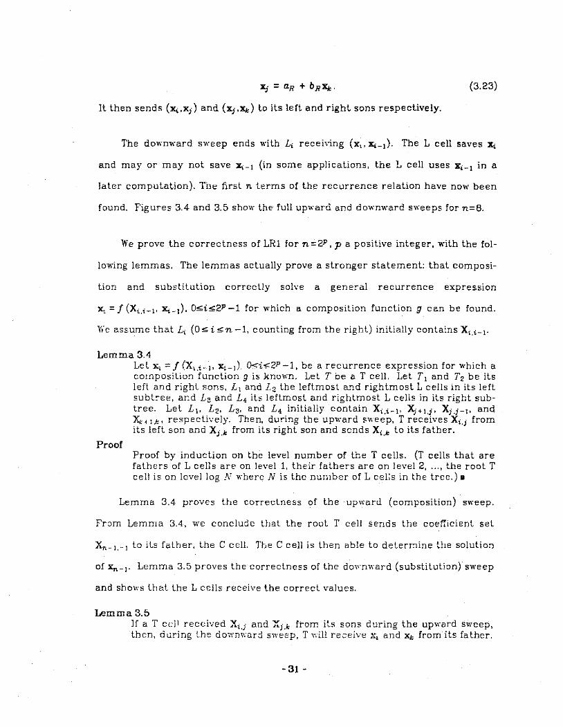
(3.23)

It then sends (x..xj) and (Xj,x,) to its left and right sons respectively.

The downward sweep ends with L; receiving (x,, x,_ 1). The L cell saves X;

and may or may not save Xi-! (in some applications, the L cell uses x,_ 1 in a

later computation). The first n terms of the recurrence relation have now been

found. Figures 3.4 and 3.5 show the full upward and downward sweeps for n=B.

We prove the correctness of LRl for n=2P, p a positive integer, with the fol-

lowing lemmas. The lemmas actually prove a stronger statement: that composi-

lion and substitution correctly soh·e a general recurrence expression

X;= f (X;,;_ 1, x,_1), Q,;;i,;;2P -1 for which a composition function g can be found.

We assume that L; (0,;; i ,;;n -1, counting from the right) initially contains Xu-I·

Lemma 3.4

Proof

Let x, =f(X;.i-Jo x,_,), O,;;i,;2P-1, be a recurrence expression for which a composition function g is known. Let T be a T cell. Let T 1 and T2 be its left and right sons, L 1 and L 2 the leftmost and rightmost L cells in its left subtree, and L 3 and £ 4 its leftmost and rightmost L cells in its right sub­tree. Let £ 1, L2, L3, and L 4 initially contain X;,;_ 1, Xj+J.j• Xj.)-J• and X.+J.k• respectively. Then, during the upward sweep, T receives X,,j from its left son and Xj.k from its right son and sends X;,k to its father.

Proof by induction on the level number of the T cells. (T cells that are fathers of L cells are on level 1, their fathers are on level 2, ... , the root T cell is on level log N where N is the number of L cells in the tree.) •

Lemma 3.4 proves the correctness of the upward (composition) sweep.

From Lemma 3.4, we conclude that. the root T cell sends the coefficient set

Xn-l.-J to its father, the C cell. Tbe C cell is then able to determine the solution

of Xn-J· Lemma 3.5 proves the correctness of the do•,·nward (substitution} sweep

and shows that the L cells receive the correct values.

Lemma3.5 1f a T ccl_l received Xi.i and ""Xi.k ftom its sons during the up\nJ.rd sweep, then, during lhe downward sweep, T "·ill receive x, and X;; from its father.

-31 -

Proof

Jt then uses x,., to solve for x1 and sends (x;. x1 ) to its left son and (x1, x,.,) to its right son.

Proof by induction on the level number of the T cells. (Start with the root T cell and proceed downward.) •

Lemma3.6 LR1 is correct.

Proof Follows direclly from Lemmas 3.4 and 3.5. •

The analysis of LR1 is shown in Figure 3.6. During the upward sweep, each L

cell and each T cell sends two values lo their lathers. Because there are log n

levels of T cells, the total communication time required during the upward

sweep is 2 (log n + 1) units or steps, where one unit is the time required for a

cell to send one value to an adjacent cell. Similarly, during the downward sweep,

the C cell and T cells send two values to each of their sons. The time required

during the dovmward sweep is also 2 (log n + 1) steps. Only the T cells perform

arithmetic operations. A T cell performs one addition and two multiplications

(3.22) during the upward sweep and one addition and one multiplication (3.23)

during the downward sweep. Thus, LRl requires a total of 2logn parallel addi-

tions and 3log n parallel multiplications for both sweeps.

We may use a similar algorithm to solve the first-order backward

recurrence relation

Xn-1 = an-1

Xn-2 = an-2 + bn-2Xn-! (3.24)

Called BLRl, it has the same time complexity as LRl.

-32-

Extensions We end this section by describing variations of the basic LRl algorithm.

Similar variations of FRACTJON and LR2 are also possible.

Empty L cells. If the desired number (n) of terms of the recurrence rela­

tion is not a power of 2, we must use a tree with 2P L cells where p = hog nl.

Some of the L cells will be empty and will not participate productively. When

distributing the initial coefficient pairs among the L cells, Xc.-1 is stored in the

rightmost occupied L cell, X1.o is stored in the next occupied L cell to the left,

and so on. Surprisingly, we do not need to modify the T cell algorithm described

above. We must describe. however, what the empty L cells are to do.

During the upward sweep, while occupied L cells send up their coefficient

pairs, empty L cells send up the pair (0, 1). This has the effect of defining the

"equation" stored in an empty L cell as identical to the equation stored in the

first occupied L cell to its right. A T cell does not know whether the data it

receives is from an empty or an occupied L cell. It simply performs the two

multiplications and one addition described in Figure 3.2 during the upward

sweep. If the. pair of values from one of its sons came from an empty L cell, aT

cell effectively sends the other son's values to its father. Similarly, during the

downward sweep, a T cell blindly performs the multiplication and addition

described in Figure 3.3. L;, still receives the values x1 and :x,_ 1; empty L cells

ignore the values they receive. Figure 3.7 shows the execution of LR1 for n=5 on

a lree with 8 L cells.

Sal-.:ing several independent recurrences simultaneously. The algorithm is,

in fact, more po"·erful than described in the prev·ious paragraph. If there are

enough L cells to accommodal2 tv:o or more linear recurrences (with one L cell

-33-

"ontaining at most one equation of one linear recurrence) we may solve all of

the linear recurrences simultaneously.

Lel two or more linear recurrences be stored in disjoint segments of the L

array. Each equation of each recurrence has a pair of coefficients. We distri-

bule the coefficient pairs as follows. Starting with the first equation of the first

recurrence. we distribute the coe.fficients pairs of the first recurrence one pair

to an L cell. After storing the coefficient pair of the last equation of the first

recurrence, we continue with the coefficient pair of the first equation of the

second recurrence, and so on. We ,.,-,ay consider the entire initial set of

coefficient pairs to be the terms of one large linear recurrence and apply LR1 to

all of the L cells. Because the first coefficient pair of each recurrence is of the

form (a. 0), we are sure that the terms of one linear recurrence will not be

affected by the terms of another. i\"e may therefore store as many linear

recurrences as the L cells can hold, apply LRl, and in a single sweep, solve all

recurrences simultaneously.

3. Quotients of Linear Recurrences

Consider recurrence expressions of the form

Xo = ao

a, + biX.-1 x.= c, + d;x,_ 1

i=1,2, ... ,n-1. (3.25)

where c, and d; are not both 0. As "·ith first-order linear recurrences, we let

(3.26)

where b 0 = d 0 = 0, and o 0 = 1. Moreover, if

-34-

_ a+ bx; X; - c + dxi

we say that ~.i =(a, b, c, d). Therefore we may express (3.25) as

where X;.;-1 =(a.. b.,, c;. d.,.).

(3.27)

(3.28)

To determine the corresponding composition function g, we observe th~t if

and

then

=

=

The desired function is

a'+ b 'x.t x,=c'+d'x.t

a'+ b'x.t a + b -..,.--:--"­

c' + d'x.t

a'+ b'x.t c +d---..:;_

c' + d'x_

a (c' + d'x,) + b (a'+ b'x.) c (c' + d 'X.) + d (a' + b 'X.)

(ac' + ba ') + (ad' + bb ')X. (cc' + da ') + (cd' +db ')X.

g (X;.j, X;,k) = X;,k = (ac' + ba ', ad' + bb ', cc' + da.', cd' + db'),

(3.29)

(3.30)

(3.31)

(3.32)

Equation (3.2B) describes a recurrence expression whose composition func-

tion is defined in (3.32). lising Lemmas 3.4 and 3.5, we can develop a tree

-35-

algorithm, which we call FRACTJON, to solve (3.28) in one upward and downward

sweep through the tree. FRACTJON determines the first n terms of (3.28). For

ease of presentation, assume that n = 2P. L;, counting from the right, initially

contains the quadruple Xi.i_ 1 = (a.,,b;.c;.d;); the rightmost L cell contains

Xo.-1 = (ao, 0, 1, 0).

Composition starts v.ith the L cells sending Xu_ 1. AT cell receives

(3.33}

from its left son, and

(3.34)

from its right son. As described by equation (3.32), the T cell computes and

sends

(3.35)

to its father. The upward sweep ends with the C cell receiving the quadruple

(a, 0, c, 0) v:here a I c is the solution of Xn- 1, the leftmost L cell in the tree. This

ends the composition sweep.

The C cell divides a by c and returns the pair (a! c, 0) to the root T cell

starting the substitution sweep. As in LRl, the second component is the value of

the dummy variable x_ 1 and the first component is the value of x,.._ 1• The T cell

that received xi.j and xj.k from its left and right sons during the upward sweep

receives the pair (x;.X;:) from its father. It determines Xj by substituting X;: into

the equation represented by Xi.•· i.e.

a.R + bRX.

CR + dRX::

-36-

(3.36}

and sends (x,.x1) to its left son and (x1,x,) to its right son. L;, receives the pair

(x,. x,_1). Using Lemmas 3.4 and 3.5, we prove the correctness of the tree algo-

rithm FRACTJON.

Lemma 3.7 FRACTJOJ\ is correct.

Proof Follows from Lemmas 3.4 and 3.5. •

The analysis of FRACTJO?\ is summarized in Figure 3.8. During the upward

sweep, L cells and T cells send a quadruple to their fathers, requiring a total of

4log n + 4 communica\.ion steps. Each T cell also performs 4 additions and 8

multiplications. The C cell performs one division. During the downward sweep,

the C cell and the T cells send a pair of values to each of their sons, requiring a

lola! of 2log n + 2 communication steps. Each T cell performs 2 additions and 3

multiplications or di\isions.

Extensions

The variations to LRl presented in the previous section may also be applied

to FRACTJO:\ in a similar manner. To accommodate empty L cells, we program

empty L cells to send the quadruple (0, 1, 1, 0) to their fathers during the

up1'ard sweep. This has \.he effect of defining the "equation" stored in an empty

L cell as identical to the first nonempty L cell to its right. Because of the associ-

ati>ily property enjoyed by the composition functions, this has no effect on the

nonemply L cells. A T cell need not know whether the information it receives

came from an empty or a nonempty L cell.

-37-

4. Second- and Higher-order lJnear Recurrences

Composition and Substitution may be extended to higher-order

recurrences. We present the tree algorithm LR2, the solution for the first n

terms of a second-order linear recurrence; the generalization to third and

higher-order recurrences is straightforward. Given

Xo = ao + box_, + CoX-z

x1 = a 1 +b 1:xo+c 1x_ 1

Xz = az + bzXt + c2Xo (3.37)

where x_1 and x_2 are dummy variables and b 0 =c 0=c 1=0. we want to solve for x,.

Osisn -1. Equation (3.37) is of the form

x, = I (Xu-t.i-2· x,_,, X;-z) . (3.38)

In order to find a composition function g which satisfies equation (3. 7) we use a

change of variables. Define

rx, 1 ral rbcl y, = [x,_, j A,= [ 0' J B; = [; 0' J and Xi.i- 1 =(A;. B;) (3.39)

for Osi :s;n-1. Equation (3.37) may therefore be expressed as

Y; = A; + B,y,_, = f (Xi.i-1• y,_,) (3.40)

which is a first-order linear recurrence in y. We can now use the method of Com-

position and Substitution, with scalar addition and multiplication replaced by

vector addition and matrix multiplication, provided we can find a suitable com-

position function g. Given

y, =A+ Byi = f (Xi.i• Yi)

Yi = A. + B 'y" = f (Xi.<. Y•)

-38-

(3.41)

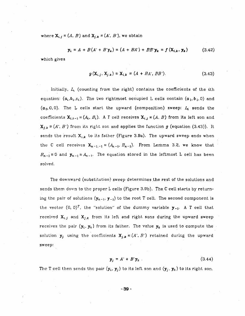
where X;,;= (A. B) and X;.k =(A', B'), we obtain

(3.42)

which gives

g(X;J• X;.<)= X;,k =(A+ BA', BB'). (3.43)

Initially. L.. (counting from the right) contains the coefficients of the ith

equation: (eL;.b;,c;). The two rightmost occupied L cells contain {a 1, b 1, D) and

(a 0 , D, D). The L cells start the upward {composition) sweep: L; sends the

coefficients X1,,_1 =(A;. B1 ). A T cell receives X;,;= (A. B) from its left son and

X;.• =(A', B') from its right son and applies the function g (equation {3.43)). It

sends the result X,,k to its father (Figure 3.9a). The upward sweep ends when

the C cell receives Xn-1.- 1 = (An_1, Bn_ 1). From Lemma 3.2, we know that

Bn_1 = D and Yn- 1 = An- 1. The equation stored in the leftmost L cell has been

solved.

The downward (substitution} sweep determines the rest of the solutions and

sends them dovm to the proper L cells (Figure 3.9b}. The C cell starts by return­

ing the pair of solutions (Yn- 1, y _1) to the root T cell. The second component is

the vector (D, D)T, the "solution" of the dummy variable y _1. A T cell that

received X,,1 and X;.• from its left and right sons during the upward sweep

receives the pair (y;, Y<) from its father. The value Y• is used to compute the

solution Y; using the coef!icients X;.k =(A'. B') retained during the upward

sweep:

Y; =A'+ B'y• (3.44)

The T cell then sends the pair (y1 , Y;} to its left son and (y1 , y.) to its right son.

-39-

L; receives the pair (y,, y,_ 1). In effect, L, receives the solutions x,. x,_1, and

X.-E· This ends the do"·nward sweep.

A proof similar to that of Lemma 3.6 suffices to show the following.

Lemma 3.6 LR2 is correct. •

The analysis of LR2 is shown in Figure 3. 10. During the upward sweep, each

T cell receives 6 values, the components of the pair (A, B). from each son, and

sends 6 values to its father. The number of communication steps is therefore

6log n + 6. During the downward sweep, each T cell receives 4 values, the corn-

ponents of the solution pair {y,, Yk) from its father and sends 4 values to each of

its sons. The number of communication steps is 4log n + 4. Only the T cells

perform arithmetic operations. During the upward sweep, each T cell must

apply the function g (equation (3.43)). This requires 12 multiplications and B

additions. As there are log n levels ofT cells, a total of 12log n parallel multipli-

cations and Blog n parallel additions are required. During the downward sweep,

each T cell must solve equation (3.44). This requires a total of 4log n rnultiplica-

lions and 4log n additions.

Extensions

If some of the L cells are empty, we program an empty L cell to send up the

pair (A, B) where

(3.45)

The effect is to define the "equation" stored in the empty L cell as identical to

the equation stored in the first nonempty L cell to its right. Because of the

-40-

associativity property of g, this has no effect on the solution process.

Extending the method of Composition and Substitution to higher-order

linear recurrences is straightforward. To solve a kth-order linear recurrence,

we transform the original equations into a linear recurrence with matrix

coefficients as we did in equation (3.39). Vie then use a tree algorithm analogous

to 1Rl. The resulting coefficients, however, will include (k x k) matrices and the

T cell operations will involve multiplying these matrices. Each T cell, therefore,

will need O(k 2) storage and will perform O(k 3) arithmetic operations. Jn order to

solve the tridiagonal and block-tridiagonal linear systems described in this

dissertation, we need to solve only first- and second-order linear recurrence-s,

which, as has been shown above, can be done with cells with very modest storage

capacity.

C. Atomic Rotate Left: RDTLA

Backus [Back7B] describes the functions rotate left (ROTL) and rotate right

(ROTR) which circularly rotate a vector of elements to the lefl and to the right,

respectively. ROT1 is defined as follows:

ROT1: x = x = <xc> --> <Xc>;

x = <Xc. x 1, • • • , Xn- 1> & n ;;, 2 --> <x1• · · · , Xn-!• Xc> .

We describe three possible ways of implementing ROT1 on a tree machine.

Let the vector elements be distributed among the 1 cells, with the L;. (counting

from the lefl) containing X;. The first implementation sends Xc up to the C cell

and down to the right of the the 1 cell tbat contains Xn-I• as shown in Figure

3.11. Only one value must travel up to the C cell and back down again; thus, the

-41-

time required is 2log n + 2 steps. This technique is simple but it requires an

empty 1 cell on the right of x,._ 1. The second implementation avoids this prob­

lem by sending all of the values up to the C cell and broadcasting them back

down. L;. is programmed to receive the value X;+J{moan) when it arrives. This

method always works, not only for ROT1, but for an arbitrary permutation. The

disadvantage is that (2logn + 2) + (n-1), or O(n), steps are needed.

A third implementation is described by Presnell [PrPaBl]. This tree algo­

rithm, called ROTLA, enables L; to receive X.+!(moa n) (avoiding the storage

management problem of the first implementation) but requires only 2Jogn + 2

steps. One drawback is that ROTLA works only if the elements are atoms (single

numbers or characters), or a small fixed-length vector of atoms, such as a pair

of atoms representing a complex number whereas the function ROT1 allows the

x;'s to be arbitrary sequences. The analogous algorithm ROTRA implements the

function rotate right (ROTR) with the same restrictions.

After some use, it became apparent that ROTLA could also be used to pro­

vide a means of communication among the 1 cells. Because the L cell that ini­

tially contains x.; receives X.+J{mod n) this algorithm may be used for vector

operations that need to combine x.; and x.;., (mod n)· As a communication tool,

ROTLA gains power if some of the 1 cells can be masked from the operation at

appropriate limes. This allows the user to specify different subsets of 1 cells

and to have members of a subset communicate exclusively among themselves.

This potential use of ROTLA is the primary reason for including it in this disserta­

tion.

-42-

ROTLA is an example of a permutation that can be implemented on a tree

machine in O(log n) time. This is not true of all permutations. For example, if

the tree is full (all of the L cells are occupied}, the time required to reverse the

order of the elements of a sequence is linear. Reversal and other permutations

on a tree machine were studied by Tolle and Siddall [ToSiBl].

We now describe ROTLA. We are given x=<XQ.X1, · · · ,x,._1> and wish to

obtain x=<x1. · · · ,x,._1 ,XQ>. Some of the 1 cells may be empty. L, (counting

from the left} initially contains x.;.

The L cells begin the upward sweep by sending up their x-values; empty L

cells send up the distinguished symbol ¢. Every T cell receives a value from

each of its sons and sends one of the values to its father as specified by the fol-

lowing code:

L.receive(LVAL}. R.receive(RVAL}; if 1\'AL>"¢ then f'.send(LVAL} else F.send(R\'AL}

The second line of code states that the T cell should send the value received

from the left son provided it is not the empty symbol ¢. Otherwise, it should

send the value received from the right son. The upward sweep ends when the C

cell receives a value from the root T cell; this value is Xc· the leftmost vector ele-

ment. Figure 3.12 shows the upward sweep for ROTLA with n=5 on an eight-1-cell

tree machine.

The downward sweep begins when the C cell returns Xc to the root T cell.

Each T cell receives one value from its father and sends one value to each of its

sons as specified by the following code. LVAL and RVAL. the values received from

the T cell's lefl and right sons during the upward sweep. were stored in the T cell

-43-

for use during the downward sweep.

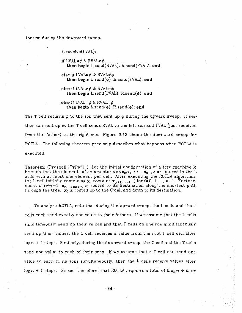
F.receive{FVAL);

if LVAL;t¢ & RVAL¢¢ then begin L.send{RVAL), R.send{FVAL); end

else if LVAL=¢ & RVAL;t¢ then begin L.send(¢). R.send(FVAL); end

else if LVAL;t¢ & RVAL=¢ then begin L.send{FVAL), R.send(¢); end

else if LVAL=¢ & RVAL=¢ then begin L.send(¢), R.send{¢); end

The T cell returns ¢ to the son that sent up ¢ during the upward sweep. If nei­

ther son sent up ¢. the T cell sends RV AL to the left son and FV AL {just received

from the father) to the right son. Figure 3.13 shows the downward sweep for

. ROTLA. The following theorem precisely describes what happens when ROTLA is

executed.

Theorem: (Presnell [PrPa!31)) Let the initial configuration of a tree machine M be such that the elements of ann-vector x=<:xa.x1, · · · •Xn- 1> are stored in the L cells with at most one element per cell. After executing the ROTLA algorithm, the L cell initially containing x, contains X(i+l) mo~ "' for i=O: 1, ... , n-1. Further­more. if i¢n -1, X(i+l) mod n is routed to its destination along the shortest path through the tree. Xo is routed up to the C cell and down to its destination.

To analyze ROTLA, note that during the upward sweep, the L cells and the T

cells each send exaclly one value to their fathers. If we assume that the L cells

simultaneously send up their values and that T cells on one row simultaneously

send up their values, the C cell receives a value from the root T cell cell after

log n + 1 steps. Similarly, during the downward sweep, the C cell and the T cells

send one value to each of their sons. l_f we as"ume that a T cell can send one

value to each of its sons simultaneously, then the L cells receive values after

logn + 1 steps. We see, therefore, that ROTLA requires a total of 2logn + 2, or

-44-

O(log n}, parallel communication steps. The analysis of ROTLA is summarized in

Figure 3.14.

If X. is not atomic, but rather a vector of length k, we can use the same

technique but simply consider the k elements to be a single data item if the k

elements can be stored in a single 1 cell. Because the T cells can pipeline their

operations, the total time required is 2log n + 2 + (k - 1 }, which is still O(log n}

if k « logn.

D. General Data Communication Algorithm: GDCA

1. Description

ROTLA circularly shifts the values of the occupied 1 cells a distance of 1 to

the left. lihen constructing algorithms for a tree machine, the need for other

data communication techniques quickly arises. For this purpose, we describe

GDCA. We define a communication pattern to be a pair <o:. (3>, where o: and {3

are the mappings of data items onto the 1 array before and after "communica­

tion," where a mapping is a 1-1 function from a set of values !:xa. x1, ... , Xn-d

onto the set of 1 cells !L0 , L 1 • ... , Ln-d· Before communication, each occupied 1

cell must contain a value, its index, and the value of its index after communica­

tion. This means that only communication patterns in which {3 is easily com;mt­

able in terms of o: are of practical interest, using information such as the index

of the 1 cell, the number of values, row and column numbers associated with the

values (for data obtained from a matrix), etc. For example, we may want to shift

the L cell values a distance k> 1 (Figure 3.15a}. (We could do this with k applica­

tions of ROTLA but GDCA is mo:-e efficient.} As another exC~mple, we may want L;.

-45-

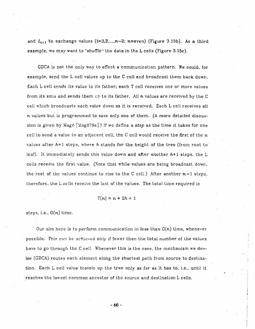
and Li+ 1 to exchange values (i=0,2, ... ,n-2; n=even) (Figure 3.15b}. As a third

example, we may want to "shutne·· the data in the L cells (Figure 3.15c}.

GDCA is not the only way to effect a communication pattern. We could, for

example, send the L cell values up to the C cell and broadcast them back down.

Each L cell sends its value to its father; each T cell receives one or more values

from its sons and sends them en to its father. All n values are received by the C

cell which broadcasts each value down as it is received. Each L cell receives all

n values but is programmed to save only one of them. (A more detailed discus­

sion is given by Mag6 [l.lag679a].) If we define a step as the time it takes for one

cell to send a value to an adjacent cell, the C cell would receive the first of the n

values afler h+ 1 steps. where h stands for the height of the tree (from root to

leaf). It immediately sends this value down and after another h+ 1 steps, the L

cells receive the first value. (Note that while values are being broadcast dovm,

the rest of the values continue to rise to the C cell.) After another n-1 steps,

therefore, the L cells receive the last of the values. The total time required is

T(n} = n + 2h + 1

steps, i.e., O(n} time.

Our aim here is to perform communication in less than O(n} lime, whenever

possible. Thi' can be achieved only if fewer than the total number of the values

have to go through the C cell. Whenever this is the case, the mechanism we dev­

ise (GDCA} routes each element along the shortest path from source to destina­

tion. Each L cell value travels up the tree only as far as it has to, i.e., until it

reaches the lm,·est common ancestor of the source and destination L cells.

-46-

The basic idea of this mechanism is that each T cell constructs a 4-register

directory (LLOW, LHJGH, RLOW, R.l-ilGH) containing the sequence numbers of the

leftmost occupied L cells in its left and right subtrees (LLOW and RLOW), and the

rightmost occupied L cells in its left and right subtrees (LHIGH and RHJGH). If

all of the L cells of the left subtree are empty, then LLOW and LHIGH are ¢. The

same is true for the right subtree. ln a sense, the machine determines o. (what

is where in the machine before communication). {3 is determined as follows.

When an L cell wants to send information, it determines the sequence number of

the recipient L cell (DEST#) and sends the pair (DEST#, VALUE) to its father T

cell. AT cell compares DEST# with the information in its directory to determine

whether to send the pair (DEST#. VALCE) further up the tree or down to one of

the sons. L cells communicate by sending· the pair (DEST#. VALUE). The T cells

route the data left, right, or up as soon as the data is received. This algorithm

sends an L value only as far up the tree as necessary, thus making most efficient

use of the tree branches. The maximum distance a value must travel from one L

cell to another is lv.ice the height of the tree.

Constructing the directories is straightforward and can be done in a single

upward and downward sweep. ln the upward sweep, empty L cells send a "0" to

their fathers, occupied L cells send a "1". AT cell receives values from its left

and right sons into 1"\t:M and RKUM and sends LNt:M+RNUM to its father. Ll\UM

and Rl\t:M contain the number of occupied L cells in the T cell's left and right

subtrees. The C cell receives from its son a value n which equals the total

number of occupied L cells in the tree as shown in the example of Figure 3.15a.

The C cell starts the dm"nward sweep by retur!:ling nand n-1 to its son, the

root T cell. Each T cell constructs its directory using the algorithm shown in

-47-

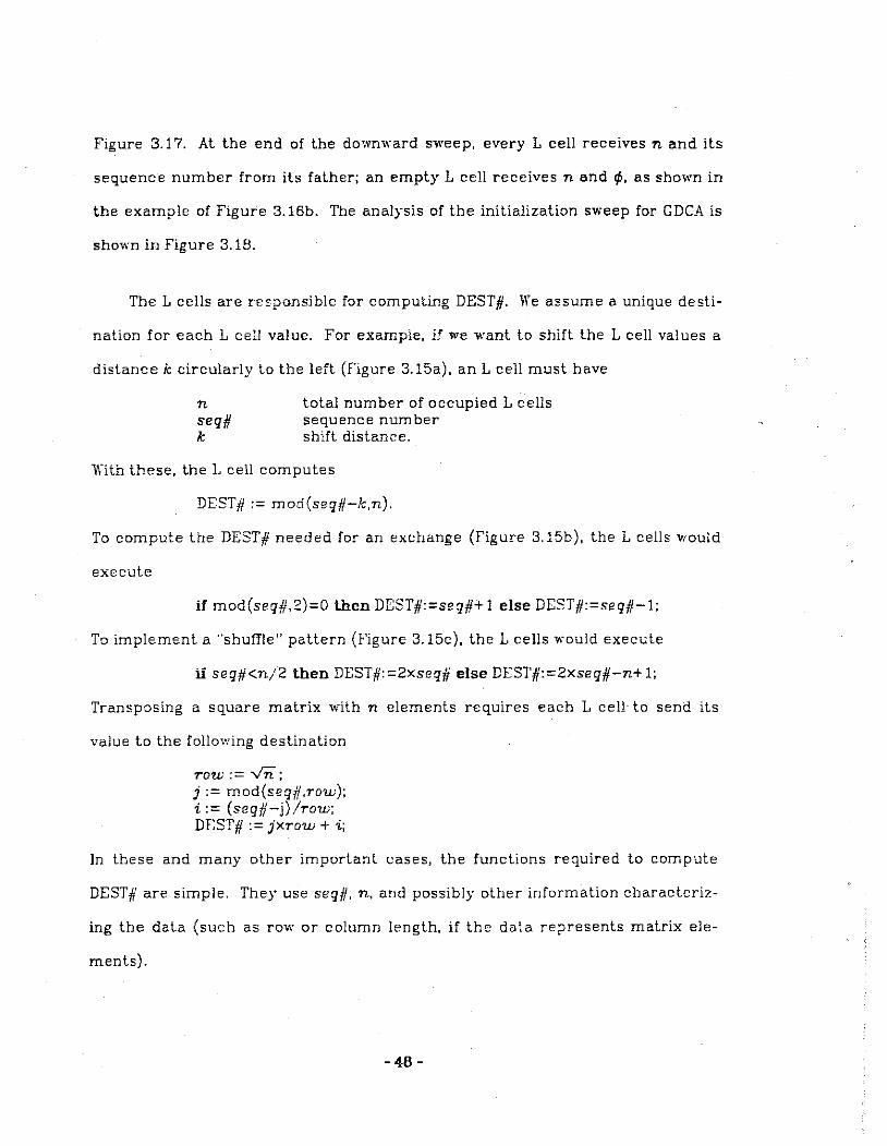
Figure 3.17. At the end of the downward sweep, every L cell receives n and its

sequence number from its father; an empty L cell receives nand ¢. as shown in

the example of Figure 3.16b. The analysis of the initialization sweep for GDCA is

shown in Figure 3.18.

The L cells are recponsible for computing DEST#. We assume a unique desti-

nation for each L cell value. For example, if we want to shift the L cell values a

distance k circularly to the left (figure 3.15a), an L cell must have

n seq# k

total number of occupied L celts sequence number shift distance.

Viith these, the L cell computes

DEST# := mod(seq#-k,n).

To compute the DEST# needed for an exchange (figure 3.15b), the L cells would

execute

if mod(seq#.2)=0 then DEST#:=seq#+ 1 else DEST#:=seq#-1;

To implement a "shuffle" pattern (Figure 3.15c), the L cells would execute

if seg#<n/2 then DEST#:=2xseq# else DEST#:=2xseg#-n+ 1;

Transposing a square matrix with n elements requires each L cell to send its

value to the following destination

TOW:: vn; j := mod(seq#,row); i := (seq#-j)/row; DEST# := jxrow + i;

In these and many other important eases, the functions required to compute

DEST# are simple. They use seq#. n, and possibly other information characteriz-

ing the data (such as row or column length, if the data represents matrix ele-

ments).

-46-

The time required to perform GDCA, however, would depend on what the

communication pattern is. Some patterns would still require O(n) time. For

example, reversal of the L cell elements (for an n L cell tree machine, sending

the contents L, to 4.-i-l• i= 0, 1 ... ., n-1) would require all of the L cell elements

to go through the root T cell, i.e., O(n) execution time. The "shuffle" pattern

(Figure 3.15c) and transposing a square matrix with n elements also require

O(n) time. Some patterns, however, are subli.near, such as the k-shift and

exchange patterns shown in Figures 3.15a and 3.15b.

In this dissertation, we shall often make use of GDCA, especially to perform

k-shifl. The next seclion presents estimates of the execution time of GDCA when

performing a k-shifl.

. 2. Execution Time of K-shiil

first, we develop an upper bound of the time required by GDCA t.o perform a

circular k-shift to the left. The analysis of a k-shift to the right is similar. Let

N = 2P be the number of L cells and n the number of occupied L cells (i.e., the

number of 1 cells participating in the shift). We analyze only values of k,;; fn; 21.

(A k-shift to the left, where k > h; 21. is equivaled to an (n-k )-shift to the right,

where n -k,;; fn I 21. By symmetry, the analysis of an (n -k )-shift to the right is

idenl!cal to a /c -shift to the left.) Define the le"Uel of a cell to be the length of the

shortest path from the cell to any leaf. Thus, the L cells are on level 0, their

father T cells an: on level 1, ... , and the root T cell is on level p.

The T cell needs a policy to handle possible contention among its father and

sons. Conlention occurs vchen, for example, a T cell receives a DEST# from each

of its sons, and both DEST#'s must be sent to the father; the T cell must decide

-49-

which to send first. A T cell policy explicitly states which of its father and sons

has highest, middle, and least priority. Consider the two policies, Pl and P2:

Pl: FATHER> LEFTSON > RJGHTSON

P2: FATHER> RJGHTSON > LEFTSON.

P 1 says that, in the event of contention, the father has priority over the left son

which ha' priority ove:· the right son. P2 says that the father has priority over

the right son which has priority over the left son. Assume that the T cells adopt

policy Pl. The analysis using policy P2 is similar.

1\'e observe what happen>: in individual subtrees as (DEST#. VALUE) pairs are

sent up the tree. Let T be an arbitrary T cell. Let n 1 and nR be the number of

occupied L cells in its left and right subtrees, respectively. There are three

cases.

(1) k:;, n1 + np (Figure 3.19a). Because the shift distance is greater than the

number of occupied L cells in both subtrees, all of the n 1 + nR pairs must be

sent to the father of the T cell, i.e., shifted out of this subtree. Because Tis

using policy P 1. pairs from the left son are sent before pairs from the right

son. There is contention in this T cell (pairs from the right son must wait),

but no unnecessary delay.

(2) k ,;;n1 (Figure 3.19b). Because the shift distance is less than the number of

occupied L celis in T's left subtree, only the pairs from the leftmost k occu­

pied L ceils of T's left subtree must be sent to the father. The destinations

of all other occupied L cells (in T's subtrees) are in T's subtrees, and are

sent do·wn by T as soon as they are received. There is no contention;

streams flo" through the channels unencumbered. The root T cell is a spe-

-50-

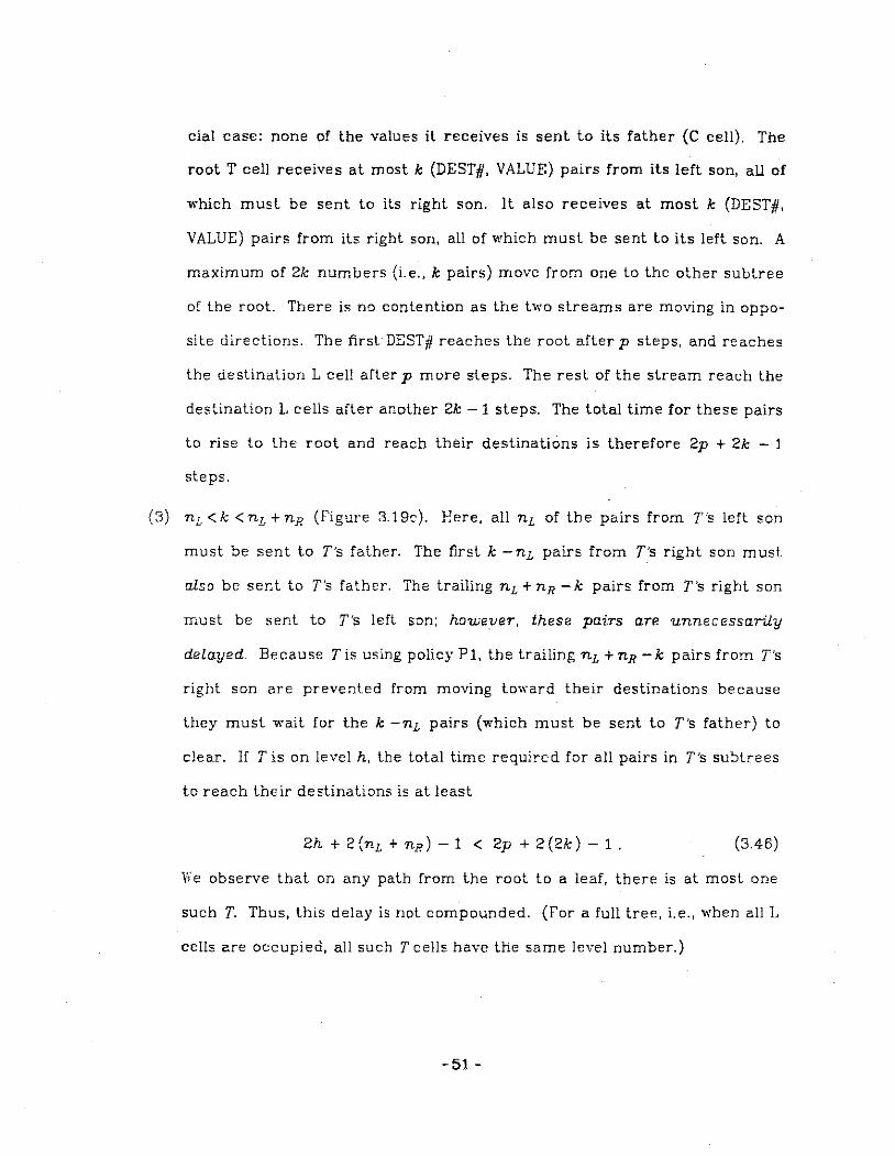
cia! case: none of the values it receives is sent to its father {C cell}. The

root T cell receives at most k {DEST#. VALUE} pairs from its left son, all of

which must be sent to its right son. It also receives at most k (DEST#,

VALUE) pairs from its right son, all of which must be sent to its left son. A

maximum of 2k numbers (i.e., k pairs} move from one to the other subtree

of the root. There is no contention as the two streams are moving in oppo­

site directions. The first DEST# reaches the root after p steps, and reaches

the destination L cell after p more steps. The rest of the stream reach the

destination L cells after another 2k- 1 steps. The total time for these pairs

to rise to the root and reach their destinations is therefore 2p + 2k - 1

steps.

(3) nL <k <nL +nR (Figure 3.19c}. Here, all nL of the pairs from T's left son

must be sent to T's father. The first k -n1 pairs from T's right son must

also be sent to T's father. The trailing nL + nR -k pairs from T's right son

must be sent to T's left son: however, these pairs are unnecessarily

delayed. Because Tis using policy P1, the trailing n 1 +nR -k pairs from T's

right son are prevented from moving toward their destinations because

they must wait for the k -nL pairs (which must be sent to T's father) to

clear. If Tis on level h, the total time required for all pairs in T's subtrees

to reach their destinations is at least

2h + 2 (nL + nR) - 1 < 2p + 2 (2k) - 1 . (346)

We observe that on any path from the root to a leaf, there is at most one

such T. Thus, this delay is not compounded. (for a full tree, i.e., when all L

cells are occupied, aJI such T ceJls have the same level number.)

-51-

We use the right hand side of (3.46), added to the time required to build the

directories (2p + 3, as shown in Figure 3.18), to bound the total time, T(k ),

required for a GDCA k-shifl, i.e.,

T(k) = (2p + 3) + 2p + 2 (2k) - 1 = 4p + 4k + 2 (3.4 7)

or O(k) time. Jf k =0 (1 cell values are not communicated), the only cost would

be the time required to initialize the T cell directories:

T(O) = T(n) = (2p + 3) (3.48)

l\ote that the problem described in case (3) would not have occurred had T

used policy P2 inste~d (rigure 3.19d). This is because the pairs (sent by T's

right son) that need to be sent to T's left son are received by T first. Hence,

they are not delayed.

A program was written to simulate a tree machine executing the GDCA k­

shifL pattern. The program was written in P1/C and run on an IB~f 360/75. The

object was to count the number of communication time units needed to execute

k-shift. The assumptions of the program were as follows.

(1) A cell could communicate with its father or sons in one time unit, where

communication means sending or receiving one numeric value. A T cell

could therefore send as many as three (possibly different) values and

receive three other values in one time unit. An 1 cell would need at least

two time units to send a (DEST#. VA1l:E) pair to its father.

(2) If a cell receives a value in one time unit, the cell has to wait at least until

the next time unit before sending that value.

-52-

(3) All cells operated synchronously.

( 4) The direction of the shift was to the left. A k-shift would cause L;. to receive

the value of L(i+k)mod n• where n is the number of occupied L cells.

The program had four parameters:

(1) the number of L cells in the tree machine,

(2) the number of occupied L cells,

(3) the shift distance k, and

(4) the T cell policy (both Pl and P2 were tested).

For a given simulation run, if the number of occupied L cells was less than the

total number of L cells, the empty cells were selected at. random, using the ran­

dom number generator described by Coveyou and Macpherson [CoMa67].

fie;ures 3.20-22 summarize the results obtained for a 16-, 32-, and 64-L-cell

tree machine where n is the number of occupied L cells and k is the shift dis­

tance. Entries under Pl and P2 are the number of steps produced by the simu­

lation. T(k) is the bound defmed by equation (3.4 7).

All results produced by the simulation were bounded by T(k ), using either T

cell policy P 1 or P2. ll is interesting to note, however, that for values of

k,;;: fn;2l and using policy Pl, the time required for GDCA did not increase uni­

formly with k (as they did with policy P2). Increases were in large amounts, fol­

lowed by plateaus (see, for example, figure 3.22, N =n =64, k = 17, ... ,31). The

values of k which cause these sudden rises correspond w·ith those identified as

potential problems in case (3). Kote also that fork> fn;21 a similar problem

occurs when policy P2 is used. In summary, the results of the simulation (Fig-

-53-

ures 3.20-22) show that best results are obtained if the T cells use policy P2

when k,.;; fn;2l and policy Pl otherwise.

-54-

Initial: X,.e Xu Xs.2

Final: x 7

Xs

Xo.-1

Xo X-!

Figure 3.1 Initial and final contents of n=B L cells executing LRl. The ith L cell, counting from the right, initially contains the pair of values (Xi.<- 1)=(a..,b,), Os;i.,n-1. At the end of the downward sweep, the ith L cell contains the soh.:­tion components Ii and Xt-l·

X· \,)

Figure 3.2 A composition step in LRJ. During the upward sweep, a T cell receives aL and bL from its left son and an and bn from its right son. The T cell stores the values aL and bL and sends the values aL+bLan and bLbn to its father, as described in equation (3.22).

Figure 3.3 A st:bstitulion step in LRJ. During tr.e dcwncard sweep, a T cell re­ceives (%i,X;;) fro!!l its father. It car..1putes xi=a.R + bRXk ar:d se~ds {~.Xj) to its left son and (x,.x.) to its right sen. 1\'ote that an and bn werestored during the upward sweep.

-55-

x •.• x. .• x, .• x •.. Xo.-1

Figure 3.4 Valt.:es commur.icated during the upward (compositior:) sweep of LRl on a fully occt.:pied 8 L cell tree machine. Composition of two linear equations oc· curs at each of the T cells.

(x,,~x,)

x, X. X. X. x, .. x, lro

"" xs ,.. "" "' x, "" x_,

Figure 3.5 Values commur.icated during the downward (substitution) sweep of LRl. Evaluation of a new" value occurs at each of the T cells. Note that the ith L cell, counting from the right, receives the solutions I< and I;-!·

LRl .

Comm. L Parallel Operations Sweep i L cells ' T cells C cell Steps

+ X + X + X

up 2logn+21 0 0 logn 2logn o I o down 2logn+2 0 0 logn logn D I 0

Tolal i 4logn+4 I D 0 2logn I 3logn 0 I D i Figure 3.6 Ar.alysis of LR!. During the t.:pward sweep, each level of cells sends a pair of values to the next higher level. Because data fror:J the L cells must pass through logn+ !levels to reach the C cell, the UP'"ard sweep requires 2logn+2 commur:ication steps. Eacl: T cell performs two :multiplicatior:s and one addition. Because there are logn levels ofT cells, the upward sweep executes 2logn paral­lel rnulliplicalior.s and logn parallel additions. No arithr:Jelic operaticr.s are exe­cuted by the C cell or the L cells. The dowr.ward sweep is analyzed similarly.

-56-

x •. ,

X.,3 X.

"'

X,,2

X.,-1

X2,1

(a)

{b)

X1,0

X1,0

"1 "'

Xo,-1

Xo,-1 ><o

"-1

Figure 3.7 Upward and downward sweeps of LRl for n=5 on an 8 L cell tree macl:ir:e. (a) Empty L cells sel"!d t:p the pair (0, 1) while occupied L cells send up the coet:icient pair (a, b). Neither the T cells nor the C cell knows whether the data it receives came from an empty or an occupied L cell. (b) At the end of the downward sweep, an empty L cell ignores the values it receives.

-57-

FRACTION Comm. Parallel Operations

Sweep Time L cells T cells C cell

+ X + X + X

up 4logn + 4 0 0 4logn Blogn 0 1 down 2logn + 2 0 0 2logn 3logn 0 0 --Total i 6logn + 6 0 0 I 6logn lllog n I 0 1

Figure 3.8 Analysis of FRACTION. During the upward sweep, each cell must send 4 values a., b, c, and d to its father, requiring a total of 4 (Jog n + 1) communication steps. Each of the T cells must substitute the equation received from the left son into the eqt:ation received from tl::e right, requiring 8 mwliplicatior.s and 4 additions, as shown in equation (3.13). A total of l:!logn parallel multiplications and 4logn parallel additions are executed. The C cell must execute a single divi­sion. During the downward sweep, every cell sends 2 values to each of its scns, requiring a total of 2 (log n + 1) communication steps. Each T cell must solve a quotient of two linear equatJons, requiring 3 multiplications or divisions and 2 ad­ditions.

X<.t X1.•

(a) (b)

Figure 3.9 Composition and substitution applied to LR2. (a) During the upward (composition) sweep, a T cell receives Xt.t = (A, B) from its left sen and X1.• =(A', B') fror:J its right son. The T cell applies the fur.ction g (equation (3.28f)) and sends the result Xa =(A + BB', BB') to its father. (b) During the dc,n:ward (substitdion) sweep, "the T cell receives the pair of solutions (y,. Y•l from its father. It uses Y• to compwte y1 using equation (3.34) ser.ds the pair (y,. Y;) to its left son and the pair (y;, Y•l to its right son.

-56-

LR2 Comm. Parallel Operations

Sweep Time L cells T cells C cell + X + X + X

up 6logn + 6 0 0 Blogn 12logn 0 0 down 4logn + 4 0 0 4logn 41ogn 0 0

Total lOlogn +10 0 0 12log n 16!ogn 0 0

Figure 3.10 Ar:alysls of LR2. During the upward sweep, a T cell receives 6 values from each son and sends 6 values to its father. The total communication lime is therefore 6 (Iogn + 6) units. During the downward sweep, each T cell receives 4 values from· its father and sends 4 values to each son. Only the T cells perform arithmetic operations. Each T cell evaluates (3.19) and (3,20) during the upward sweep, requiring 12 multiplications and 6 additions. It evaluates (3.21) and (3.22) during the downward sweep, requiring 4 multiplications and 4 additions.

Figure 3.11 One implementation of ROTL. x, is ser:t up to the C cell and ser:t down to an empty L cell to the right of X..-t·

-59-

¢

"a

Figure 3.12 ROTLA upward sweep. The L cells initiate the upward sweep by send­ing the x values to their fathers. A T cell receh·es tl:e values "'L and :>:n from its left and right sons. saves zn. and sends :l:L to its father. The upward sweep ends when the C cell receives a value from the root T cell.

¢

Figure 3.13 RO":"LA dowr.ward sweep. Tl:e dowr.wz:rd sweep starts wl:en the C cell ret.urr£ the Yah.:e tc its son. Each T cell receives a valt;.e fro:r.1 the father, ser:ds it to the right sor., and sei:ds the vall:e saved from the upward sweep (:zn) to the left sor_. The dov·.-r~ward sweep ends when tt:e L cells receive tl:e new vah..J..es.

-60-

ROTLA

Comm. Parallel Operations

Sweep L cells T cells C cell Steps + X + X + X

up logn + 1 0 0 0 0 0 0 down logn + 1 0 0 0 0 0 0

Total ! 2logn + 2 0 0 0 0 0 0

F"~gure 3.14 Analysis of ROTLA. Each cell sends one value to its father during the upward sweep. As there are log(n.)+2 levels of cells in the tree, the upward sweep requires log(n.)+l parallel communication steps. Similarly, the downward sweep req~:ires log(n)+ 1 parallel communication steps. None of the cells execute any arithmetic operatior...s.

L cells. 0 1 2 3 4 5 6 7 8 9 10 11 12 13 14 15 send: xO xl x2 x3 x4 x5 x6 x7 xB x9 receive:

(a) x3 x4 x5 x6 x7 xB x9 xO xl x2

(b) xl xO x3 x2 x5 x4 x7 x6 x9 xB

(c) xO x5 xl x6 x2 x7 x3 xB x4 x9

Figure 3.15 Exar:1ples of data communication among the L cells for n=!C, #L cells= IS (a) L cell elements are shifted circt:larly to tl:e left a distance k=3. (b) L cell ·w.ill: seql.i.ence nl.:l:lbers i and i.+1 exchange values, i=even. (c) L cell ele­ments are "stt:Jrled''.

-61-

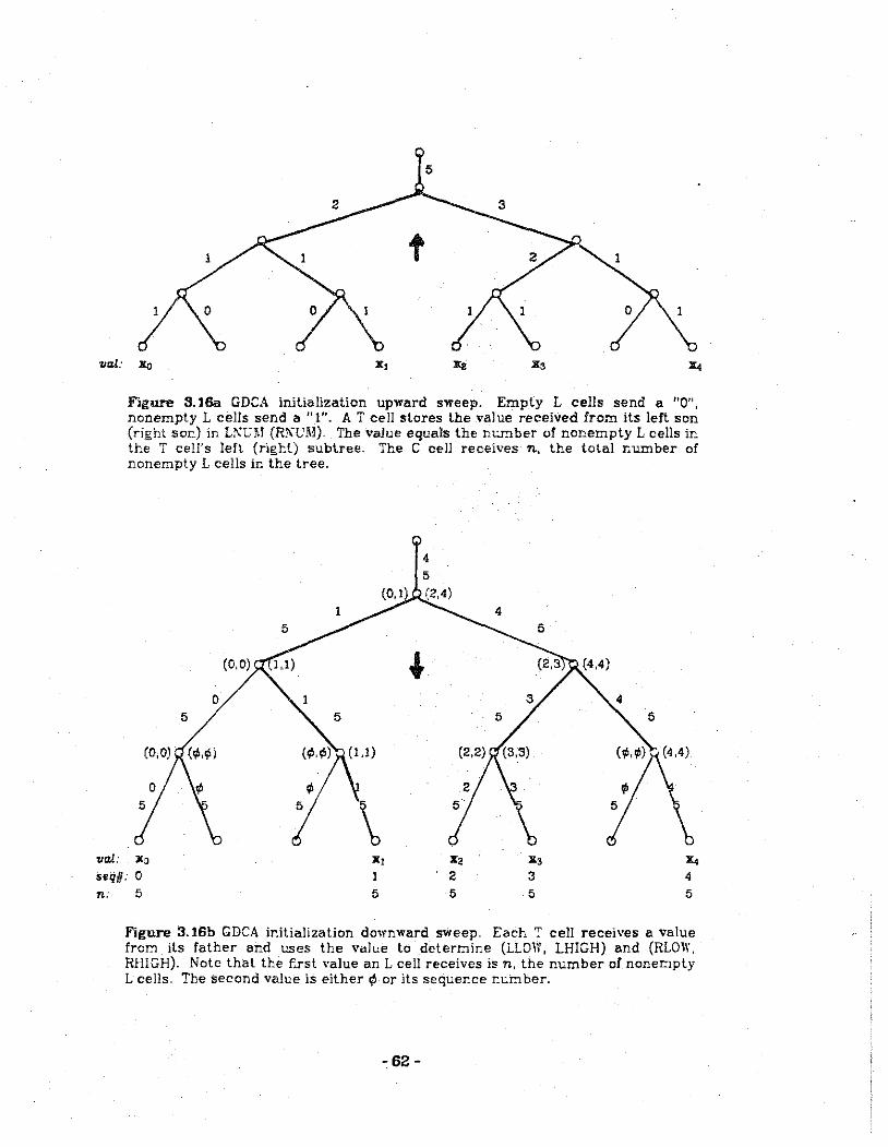
5

1 1

val: Xo "'

val:

Figure 3.16a GDCA initialization upward sweep. Empty L cells send a "0", nonernpty L cells send a"!". AT cell stores the value received from its left son (right so"-) in Ll\:GM (RJ\L'M). The value equals the number of nonernpty L cells in the T cell's lefl (rigl:l) subtree. The C cell receives n, the total number of nonempty L cells in the tree.

4 5

(2,4)

5

(0.0)

0 5 5 5

(0,0)

0 ¢ 5 5 5

Xo x, "• x, X. seq#: 0 1 2 3 4

n: 5 5 5 5 5

Figure 3.16b GDCA initialization downward sweep. Each ' cell receives a value froi'O'l its father and uses the val"e to dcteri'O'line (LLDW, LHIGH) and (RLD\\', RHIGH). Note that the f.rst value an L cell receives is n, the m.:mber of nonei'O'lpty L cells. The second value is either¢ or its sequer:ce m:.mber.

-62-

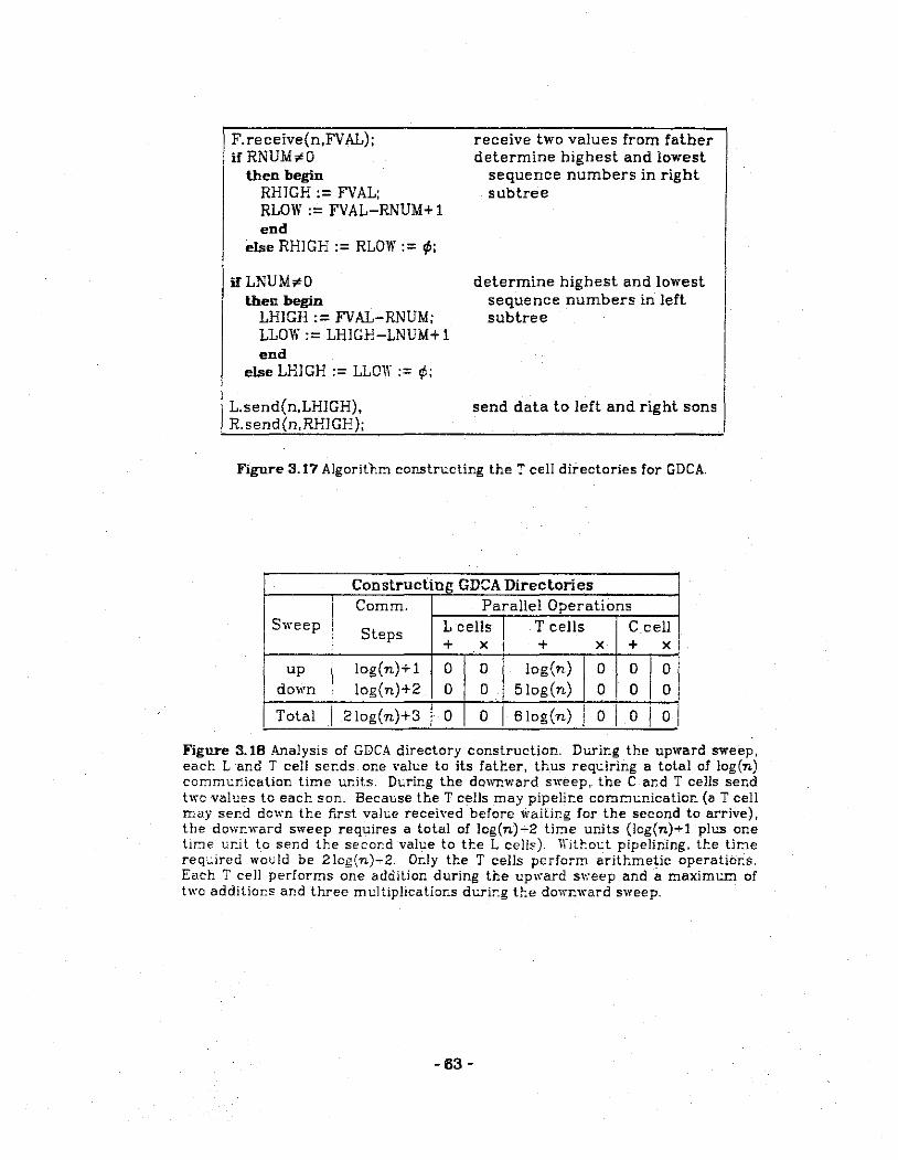
F.receive{n,FVAL); if RNUM¢0

then begin RHIGH := FVAL; RLOW := FVAL-RNUM+l end

else RHIGH := RLOW := ¢;

if LNUM¢0 then begin

LHIGH := FVAL-RNUM; LLOW := LHIGH-LNUM+l end

else LHIGH := LLOW := ¢;

I L.send{n,LHJGH), R.send(n,RHIGH);

receive two values from father determine highest and lowest

sequence numbers in right subtree

determine highest and lowest sequence numbers in left subtree

send data to left and right sons

Figure 3.17 Algorithm constructing the T cell directories for GDCA .

. ·

Constructing GDCA Directories

I Comm. Parallel Operations Sweep

I Steps 1 cells J T cells C.cell + X I + X + X

up log(n)+l 0 0 log(n) 0 0

I 0

down log(n)+2 0 0 5log(n) 0 0 0

Total 21og(n)+3 I 0 0 6log{n) I 0 I 0 I 01

Figure 3.18 Analysis of GDCA directory construction. Durir:g the upward sweep. each L and T cell ser:ds one value to its father, thus requiring a total of log(n) coomt:r1ication time ur..its. Dt:ring the dovfr..ward sweep, the C and T cells ser..d two values to each son. Because the T cells may pipelir:e ccmr.n:.nication (aT cell may ser..d down the f.l.Tst value received before \\'aitir:g for the second to arrive), the dcwr:ward sweep requires a total of Jcg(n)-2 time urJts (Jcg(n)+l plus one tioe ur:it to send the seccr:d value to tl:e L cells). Withot.:l pipelirJng. tl:e time reqc:ired would be 21cg(n)T2. Or:ly the T cells perform arithmetic operatior:s. Each T cell performs one addition during the upward sweep and a maxim= of two additior:s and three multiplications dcrir:g t!:e do•n:ward sweep.

-63-

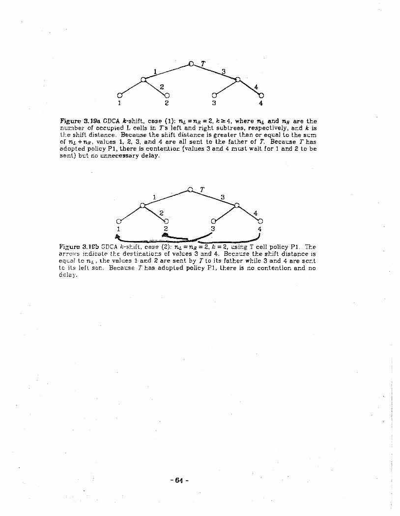
1 2 3 4

Figure 3.19a GDCA k-shift, case ( 1): 11.£ = nn = 2, k:. 4, where nL and nn are the number of occupied L cells in T's left and right subtrees, respectively, and k is the shift distance. Because the shift distance is greater than or equal to the sum of 11.£ + nn, values l, 2, 3. and 4 are all sent to the father of T. Because T has adopted policy PI, there is contentiOI: (values 3 ar.d 4 must wait for I and 2 to be sent) bt:t no unnecessary delay.

1

IL 3

...-:"'

4

4 ...)

Fi;:ure 3.1£1:> GDCA k-sr.ift, case (2): 11.£ =nn = 2, /'- 2, usir:g T cell policy Pl. Tl:e arrc••:s ir:dlcatr> ttc destir..atic:-..s of vah.:es 3 3.nd 4. Bccat.:.se the s!:.ift distance is eqLal to nL, tl:e values 1 ar:d 2 are sent by T to its fatl:er while 3 and 4 are ser.t to its left sen. Because T has adopted policy PI, tl:ere is no contentior: ar.d no delay.

-64-

1~'-----2--------3----'~4 Figure 3.19c GDCA k·shift, case (3): nL =nR = 2, k = 3, using T cell policy PI. The arrow indicates the destination of value 4. Because nL < k <nL + nR. the values 1, 2, and 3 are sent by T to its father. Value 4 should be sent to T"s left son but mcrt wait for value 3 to be sent up. Value 3, ir. turr:, must wait for values 1 and 2 to be sent up. Value 4 is, therefore, ur.necessarily delayed.

2 3 1"-.._ -------- 4 -Figure 3. !Cd CDCA k·shift, case (3): nL =nR = 2, k = 3, using T cell policy P2. The arrow ir:dicates the desti~atior: of value 4. UrJike in Figure 3.19c, value 4 is re~ ceived by T ahead of valt.:e 2. :'~t:s, 4 ffi=.y be ~_2::!. down to T's left sor.. in U:.e next tiDe step while value 2 is sent to the fatter. lr: tl:e sar::Je step, \'alues 1 and 3 are receh·ed by T. II: the r.ext two lime steps, vah:es 3 and I (in ll:al order) are sent by T to its fall:er. Vah:e 4 was not delayed.

-65-

Simulation Results (18 L cells)

n k Pl P2

4 l 20 20 2 22 22

5 l 20 20 I 2 22 1 22 3 22 I 22

8 1

120120 2 22 22

3 24 24 4 24 26

g I 1 20 lzo 2 22 22 '3 26 24 4 26 26 5 26 I 26

I jl1 1120120

2 22 22 I I 3 24 24 4 30 26 5 28 28 6 ' 28 28

12 1 20 20 2 22 22 3 26 24 4 28 26 5 30 28 6 30 ! 30

14 1 I 20 20

2 22 22 3 24 24

I 4 26 I 26

I 5 30 28

I 6 32 30

16 ' 1 I 20 i 20 I

1

12122,22 3 24 I 24

,4126 26

15132 28

,s132l3o

I 7 1

32 1 32 8 , 34 34

T(k) n

22 4 I 26 22 r 26 30 22 8 I 26 30 I 34 22

I g

26 30 ,, 34 I 38 ,, 22 li 11 26 II 30

I 34 38 42 ! 22 12 26 30 34

II 38 42 22

1141 26 30 34 I 1 38 I I 42 I I

k Pl ' P2 T(k)

3 18 16 24 4 11 ll ll

4 120 120

22 5 11 11 ll

5 24 24 30

I 6 22 22 26 7 20 20 22 I 8 ll 11 11

6 1 24 ~I

30 I 7 22 26 I 8 20 20 1 22

I 9 11 11 11

1 1 26 1 28 34 8 1 24 24 30

26 10 20 20 22 9 22i22

ll 11 11 11 I 7 28 1 26 38 ! 8 26 I 30 ;;I g 24 i 26

10 122 ' 221 26 1 ll 20 20 22 12 11 11 11 8 : 30 32 I 42 g 28 32 1 38

10 26 28 I 34 11 24 24 I 30 12 22 ' 22 I 26 13 I

20 : 20 22 14 1 1 I 1 1 I 11 9 I 32

10 J3o 11 28 12 i 26 13 ' 24 14 II 22 15 20 16 ' 11

: 321 46 I 32 42 i 32 1 38 I 2s 1 34 1 24 1 30 · 22 1 26 I 20 22 I 11 I 11

Figure 3.20

-66-

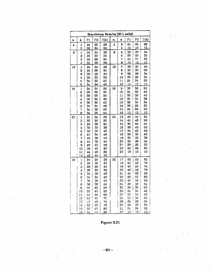
Simulation Results (32 L cells)

n k PI P2 T(k) 1/ n k PI P2 I T(k)

4~~~·~l24 22 26 II 4 I 311

241

2411

26 2 26 24 30 4 13 13 13

'1 8! I '24 241 26 8 5 128 26 34 2 26,26, 30 6,26 26 30 3 28[28 34 7'124124,26 4 30 28 38 8 13 13 I 13 ,

12 1 24 i 24 26 ' 12 1 : 32 1 3o 42 2 26 I 26 30 8 30 I 30 38 3 30 28 34 9 28,28 34 4 32 i 30 I 38

1 10 26 26~30

I ~ \ ~ I ~ :~ I ;~ I ~ j ~ I ;~ 16 I i 24 I 24 26 .,. 161 9 36 i 38 I 50

2 I 26 I 26 30 10 34 30 I 46 3128 28 34 I 11 32 32 I 42 4 36 30 38 I 12 30 34 38

I 5 38 32 42 13 2e 3o ! 34 I 6 I 38 ' 34 46 ' 14 26 i 26 'I 30

7 1

34 i' 36 1• 50 ·' 15 24 I 24 I 26

8 34 36 54 16 13 13 13

23 I 24 I 24 I 26 ! 32 I 13 I 42 I 44 I 62

II

~ ~~ 1' ~~ 11 ;~ :; ;~ ~ ;~

4 30 30 38 16 36 40 50 5 32 32 42 17 34 42 46

~ I !~ ,, : I ;~ II ;: I ;~ ;~ I ;~ 8 44 36,54 20128 28134

' 9 46 I 40 58 I 21 I 26 26 I 30 I I 0 38 I 40 62 122 I 24 24 I 26

l I II 44 42 66 23 I 13 13 13 , 12 42 . 44 10 . ·. I

I 32 .,, ~] 24 24 I 26 ,,, 321' 17 i 52 I 52 82

I 26 26

1

30 18 I 50 I 52 78 28 28 34 19 48 52 74 I

I ; I ;~ ;~ I !~ I I ~~ :~. I ;~ :~ I a 1 34 34 46 22 42 , o2 62

I 7 i 36 36 I 50 I i 23 40 I 52 58 8 ' 38 38 54 I 124 I 38 i 38 54

I 190 ': 5522 4402 I 58 25 I 36 I 36 50

I - 62 I ,, 26 I 34 j 34 46 ,I

11 . 52 44 66 27 I 32 I 34 42

112 I 52 4G I 70 I ''. 2t I 3J I' 30 38 I 13 c~ 1

48 1' 74 II 1 29 1 28 28 34 114 52 i 50 78 I 30 i 26 26 30 I 15 52 52 . 82 1\ ! 31 ' 24 I 24 26 ' 16 54 ' c4 86 , ', 3~ ', 13 ' 13 13

Figure 3.21

-67-

SimuJntion Results 64 L cella)

n k P1 P2 T(k) n k P1 P2 T(k)

16 I I 28 28 30 16 2303034 3323238 4 36 34 42 5 36 36 46

6142136 50 7 44 40 54 8384058

9 10 11 12 13

:: I 16

38 42 38 44 36 36 34 36 32 32

30 I 30 28 28 15 15

32 I 26 28 ' 30 ·i 32 17 48 58 2 30 30 34 18 54 60 3 32 32 38 19 52 56 4343442 205058 5 36 36 46 21 48 56 6 42 38 50 22 46 52 7504054 234454 8524258 244254

54 50 46 42 36 34 30 15 86 82 78

, 74 I 70

I~ I 50

9 52144 82 25 40 40

1

10 152 46 66 26 38 40 11 48 48 70 27 36 36 46

12 64 I 50 I 74 I 28 34 341 42 13 60 ' 50 78 29 32 32 38

14 56 152 I 82 I 30 30 I 30 I' 34

I 15 58 56 I 86 I 31 I 28 I 28 30 16 56 . 56 I 90 32 15 ' 15 15

48 I ~ ;~ ! ;~ I ;~ 1148

I ~~ I ~~ ~~ I ; :: . I 3 32 I 32 I 38 II 27 68 721110

4 ' 34 134 42 II 2289 6646 7722 ' !06 I 65 I 36 36 I 46 102

I 44 38 50

I ;3°21 I :5;8 ~7!4 :9~o j ~ I :~ I :~ ;: 9 I 48 44 62 I 33 I 56 74 86

10 I 64 I 46 66 I 34 54 64 82

11 I 72 I 48 70 II I 35 I 52 68 I' 78 !2 70 I 50 74 II 36 I' 50 50 74 13 i 1o I 5o 78 37 48 64 10

14172 I 52 I 82 38 146 50 66 15 8o I 56 86 39 44 68 62 16 I 76 I 56 90 40 I' 42 50 58 17 I 76 60 94 [I 41 40 46 54 18 1 74 1 62 98 42

1· 38 46 50

' 19 I 62 I 64 1 O? II 43 I 36 36 46 I 20 I 76 66 ! 1 0~ 44 34 34 I 4 2

1

21 ' 76 I 66 : 110 'I I. 45 i 32 i 32 i 38 22 ! 741· 70 i 115 1· • 46 , 30 • 30 34

I 23 I 76 72 I 118 II I 4 7 I 28 i 28 30 . 24 I 72 72 ' 122 ' 4 8 I 15 I 15 15

Figure 3.22 (continued nexl page)

-66-

Simulation Results

n k Pl [ P2 T(k) n

64 1 l 26 28 301

64 2303034 3323238 4 34 34 42 5 36 36 46 6 36138 50 7 I 40 I 40 ' 54 8'54 42156 9 54 44 62 ll

!0 54 46 66 j'J.' ]] 54 48 70 ' 12 54 50 74

]3 54152 I 1e 14 54 54 ' 82 ]5 56 • 56 1 86 16 58 1 58 . 90 n'~ee 1 eoj94 !B I' 88 I' 62 98 !9 88 64 102

1

20 88 166 1061!1 21 sa sa 110 I'

, 22 ee I 70 114 23 I 88 I 72 I 118 II 24 ~1 88

1

• 74 1 122 1•

25 88 76 !' 126 .I 26 I 88 I 78 130 ti 27 ! 88 ' 80 '1!31 il 28 ; 88 I 82 138 II' 29 : 88 84 : 142 I 30 ', 88 86

1146 •1 ~

31 1 88 88 !5o : 3~ ' 90 90 154 .:

64 L cells)

k Pl P2 I T(k)

ss!8s'8s 1

34 86 88 35 84 88 36 82 88 37 eo

1 88

38 78,88 39 76 88

40 I 74 I 88 41 72 88

j 42 I 10 I 88 I 43 ' 68 1 e8

44 66

1

, 88l· 45 64 88 46 62 I aa 47 60 ' 88 '

!50 146 142 !38 134 130 126 !22 118 114 110 106 102 98 94 90

49 ! 56 1 58 86 \4815a[as!j:

I 50 I 54 54 82 51 I 52 54 , 1a 52 I 50 54 I 74 53 I 48 54 10 54 I 46 I 54 I 66

I 55 I' 44 54 I 62 I 5s , 42 ! 421 5s

I 57 J: 40 I 40 54 58 38.38 50

I~~, ~ ;: I !~ I 61 32 32 I 38 '162130 30!34 ,63128 28! 30 i 64 15 15 15

Figure 3.22

-69-

CHAPTER 4. TRIDIAGONAL IJNEAR SYSTEM SOLVERS

A Overview

On a sequential computer, an (n xn) tridiagonal linear system of equations

can be solved in O(n) time. The traditional algorithms for solving such a system

are LU decomposition and Gaussian elimination, or the more efficient Thomas

algorithm [Ames77, Youn71]. During the last two decades, parallel algorithms to

solve tridiagonal systems have been developed for computers such as the

lLLlAC-JV, CDC STAR-100, and Tl-ASC. ln 1965, R. Hackney [Hock65] introduced

cyclic reduction. a method for solving the block-tridiagonal linear system result­

ing from the five-point approximation of Poisson's equation on a square region

(Chapter 2). Buneman proposed a slightly different version of cyclic reduction

[Bune69, BuGJ\70] that was proven to be stable although requiring more arith­

metic operations. Both are direct methods and can be implemented on a paral­

lel processor in O(log n) steps, providing a great improvement over previous

methods, both direct and iterative [Dorr70]. Moreover, both methods can be

applied to tridiagonal linear systems as well [Eock70].

Stone [Ston73a] introduced a technique called recursive doubling which can

solve lineu.r recurrences on a parallel processor of the lLLlAC-!V type in O(log n)

steps. Since the LC decomposition of a tridiagonal system can be transformed

into a problem of solving linear recurrences, recursive doubling prO\ided a third

parallel tridiagonal system solver. Stone compared these three methods

-70-

[Ston75] and concluded that, for an ILLIAC-JV type parallel processor, cyclic

reduction is preferable for the constant diagonal case whereas recursive dou­

bling is more efficient when the diagonal has arbitrary values. His analysis did

not include overhead cost such as data rearrangement. Lambiolte and Voigt

[LaVo75] included overhead cost and machine liming formulas in their analyses

of three direct methods {LU decomposition, recursive doubling, and cyclic

reduction) and three iterative methods implemented on a vector processor, the

CDC STAR-100. Among their conclusions: direct methods are superior to itera­

tive methods, and for large systems cyclic reduction is the fastest. They also

concluded that when implemented on a vector processor, recursive doubling

required O(n logn) time, compared to the O{n) lime required by traditional

algorithms on a sequential computer. This is because recursive doubling

requires a total of O(n log n) operations and a vector processor gives only a con­

slant speedup over sequential computers. Furthermore, Diamond [Diam75] has

found recursive doubling to be unstable for certain systems of equations.

Other methods subsequently developed include a method by Sameh and

Kuck [SaKu78] based on Givens' reduction of a matrix to triangular form, and a

method by Swarzlrauber [Swar79] based on Cramer's rule. Both methods run in

O(log n) lime on an n-processor machine. As noted by Ortega and Voigt in an

excellent survey [OrVo77], these methods may have merit if the stability of

cyclic redue:tion i.~ in doubt.

Traditional iterative methods for solving tridiagonal systems include the

Jacobi method, Jacobi over-relaxation (JOR), the Gauss-Seidel method, and suc­

cessive over-relaxation (SOR). Lambiolle and \'o;~;t [La\'o75] found that whereas

the Jacobi method and JOR could be efficiently implemented on a vector

-71-

processor, neither the Gauss-Seidel method nor SOR could because of the

sequential nature of the recurrence expressions produced. However, a variation

of SOR called red-black SOR [Youn71], which treats the vector of elements as

two independent halves, could be efficiently implemented. Traub [Trau73) intro-

duced a method that transforms the recurrence equations of LU decomposition

into iteralions and showed that the rate of convergence is independent of the

size of the matrix. Lambiolte and Voigt [LaVo75] implemented Traub's alga-

rilhm on the STAR-100 and an accelerated version of the algorithm is described

by Heller, Stevenson and Traub [EeST76].

This chapter addresses the problem of implementing tridiagonal linear sys-

tern solvers on tree machines. As some of the algorithms presented can be

decomposed into problems of solving first- and second-order recurrence expres-

sions, we will make frequent use of the tree algorithms LRl, LR2 and FRACTJON,

as well as the tree communication algorithms ROTLA and ROTRA, all described in

Chapter 3.

Our aim is to solve the (n xn) tridiagonal linear system

rbo co 0 1 r Xo rc a, b 1 c 1 x, r,

az bz Cz Xz = rz (4.1)

Cn-2

0 tin-! bn-l Xn-1 rn-1

Section B presents three classes of direct solution methods. The first

transforms the coefficient matrix into an upper bidiagonal matrix and solves the

new system using back substitution. This class includes Gaussian elimination

and the Thomas algorithm, algo;-ithms that appear to be inherently sequential

and, thus, have been thoughl to be unsuitable for other parallel processors

-72-

[Ston75, LaVo75, HeST76, JeHo79, OrVo77]. B.oth methods run in O(n) time on a

sequential computer and (as we show later) in O(log n) time on a tree machine.

The second class of solutions uses LU decomposition, i.e., the coefficient matrix

is decomposed into LU where L is lower bidiagonal and U is upper bidiagonal.

The system is then solved using forward substitution and back substitution. Two

examples are given, both of which take O(n) time on a sequential computer and

O(Jog n) time on a tree machine. The third class of algorithms is based on cyclic

reduction, in one step transforming a tridiagonal system into one approximately·

half its size. Iterating O(log n) times, we are left with one equation in one unk­

nown. We sol,·e this equation and, in O(log n) more iterations, solve for the rest

of the variables. This clpss includes cyclic reduction and Buneman's algorithm

and requires O(n) time on a sequential computer and O((log n) 2) time on a tree

machine.

In section C, we investigate iterative solution methods, including the Jacobi

method, JOR, the Gauss-Seidel method, SOR.. red-black SOR, and an iterative

analog to LU decomposition developed by Traub [Trau73]. One iteration of each

of these methods requires O(n) time on a sequential computer and O(log n) time

on a tree machine.

In section D, we summarize our results and make comparisons with results

obtained by Stone [Ston7C>] on a parallel processor and by Lambiotte and Voigt

[LaVo75] on a vector computer.

-73-

B. Direct Methods

1. Traditionally Sequential Algorithms

ln this section, we describe two algorithms, Gaussian elimination and the

Thomas algorithm, originally designed for sequential processing. These alga-

rithms have been considered unsuitable for efficient implementation on parallel

processors such as vector computers [LaVo75] and array processors of the

lLLJAC-IV type [Ston75]. We will see that they can be implemented efficiently on

a tree machine.

Gaussian elimination and the Thomas algorithm transform (4.1) into an

upper bidiagonal system and then determine the x-vector using back substitu-

tion. Both methods use first-order recurrence expressions to obtain the bidiag-

anal system and to perform back substitution.

Thomas Algorithm

The Thomas Algorithm transforms (4.1) into.

[ 1 ec 0 1 f

Xo Yo 1 e, x, Y1

= (4.2) 1 en-2 Xn-z Yn-2

0 1 Xn-1 Yn-1

where

-74-

and

eo= colbo e; = c;l(b,-a,e,_ 1)

ci + Oei-1

bi-aiei-1 =

Yo = ro/ bo

(4.3} i= 1,2, .... n -1

i=l,2, ... n-1 (4.4)

Baok substitution provides the desired vector x:

Xn-1 = Yn-1 i=n-2, n-3, ... ,0

(4.5)

To implement this algorithm on the tree machine, we store all information

pertinent to the ith equation in the ith L cell (4). Each L cell, therefore, con-

tains

a,b,c,r e,y X

seq# t,

coefficients of one equation storage for intermediate values solution of one equation L cell's sequence number, Osseq#Sn -1 temporary

where, by definition, a 0 =cn_ 1=0. The tree algorithm proceeds as follows.

(1) Compute e, according to (4.3) using FRACTJO~. L, sends up the quadruple

(c,.O.b,.-a,) and receives (e,,e,_1).

(2) Compute y, according to (4.4) using LRLKote that all of the components of

the denominator of (4.4) are kno.,·n. The denominator may, therefore, be

evaluated by the L cells beforehand: L, computes t,:=b,-a,e,_ 1• This

reduceo (4.4) to a first-order linear recurrence in y, which is solved using

LRl with L, sending up lhe pair (rj t,, -a,! t;), and receiving y,_1 andy,.

-75-

(3) Compute X; according to (4.5) using BLRl. L, sends up the pair (y,.-e,) and

receives x,_1 and x,.

The analysis of the Thomas algorithm is summarized in Figure 4.1. This algo­

rithm requires O(log n) time to execute.

Ga.ussian Elimination

In Gaussian elimination, (4.1) is transformed into

·where

l 0

de = bo

d; = b; -a.; c, -1/ r4-I

-a..:ci-1 + bidt-1 = 0 + ld,_,

Yo= ro

y, = r, -(a, I r4- 1)y,_,

0 l [ Xc :x,

d.,. -2 Cn-2 Xn-2

dn-1 Xn-1

i=1,2, ... ,n-1

i=1,2, ... ,n-1

Back substitution provides the desired vector x:

Xn-1::: Yr.-1/dn-1

x, = (y, -c, x, + 1)/ d, i=n-2, n-3, ... ,0

The tree algorithm is as follows.

=

{1) Use ROTRA to send c,_ 1 {contained in L,_1) to L,.

Yo y,

(4.6)

Yn-2

Yn-1

(4.7)

(4.8)

(4.9)

(2) Use fRACTJOK to dclcrmin= d.; according to (4.7). L; sends up the quadruple

-76-

(3) Use LRl to determine y, according to (4.8). L, sends up the pair

(r,,-a.J d,_,) and receives y,_, andy,.

(4) Use BLRl to determine X; according to (4.9). L; sends up the pair

(y;/ d,,-c,! d;,) and receives X; and X.+!·

The analysis of Gaussian elimination is summarized in Figure 4.2. This algorithm

requires O(log n) lime to execute.

2. LU Decomposition

The LU decomposition of the matrix A, if one exists, transforms A into a pro-

duct of lov.·er and upper bidiagonal matrices. Thus

[ 1

l, 1

A= LU = lz

0

where

uc :.:. be

l, = rLJ u,_, ui = bi -lici-t

= bi - aici-11 u"i-1

\,- . L (' l .-. 1 e rev1n e ..,_ _ 1 1 as

uo = be

u. =

l, =

-a~ci-l + biv.i-1

O+lui-I

1

0 J f Uo co

I u,

ln -I 1 l 0

i=1.2, ... ,n-1

i=1,2, ... ,n-1

;.= 1,2, ... ,n -1

-77-

0

c, ( 4.10)

Un-2 Cn-2

Un-!

( 4. 11)

(4.12)

(4.13)

which expresses u'i. as a quotient of two linear functions of ui-I• and l1. as a func-

tion of U..· We solve LUx=Ly=r using forward substitution to obtain the inter-

mediate vector y,

Yo= ro Y; = r; - l;Y;-l i= 1,2 .... ,n -1

(4.14)

and back substitution to obtain the desired vector x:

X,,-1 = Yn-l/Un-1

x; = (y;- c;x;+l)/u; i=n-2, n-3, .. .,0 ( 4.15)

In the tree implementation of this algorithm, each L cell holds the following

variables:

a,b ,C ,T

l,u,y X

seq#

coefficients of one equation storage for intermediate \'alues solution of one equation L cell's sequence number, O;;.seq# ;;,n -1

where, by definition, a 0=cn_ 1=0. The algorithm proceeds as follows.

(1) l'se ROT)"i,\ to sEnd C;- 1 (contained in L;- 1) to L;.

(2) Compute u.. according to (4.12). Use FRACTIO:\ with L; sending up the qua-

druple (-a;c;_ 1, b;. 0, 1) and receiving u;_ 1 and u;.

(3) I; compute; l; according to (4.13) using u;_ 1 obtained in step (2).

(4) Compute y; accordmg lo (4.14). Use LR1 with Li sending up the pair (r;.-1;}

and receiving y1 _ 1 and Yi·

(5) Compute x, a~cording to (4.15). Fse IJLR1 with L; sending up the pair

The analysis of Lt: decomposition is summarized in Figure 4.3. This algorithm

requires O(log n) tim 2 to execute.

-76-

A 1!.elhod Using S:::cond-Qrdcr Linear Recurrences

A basic principle of the theory of continued fractions [Wall48] provides

another way to obtain U; (4.12). first solve the second order linear recurrence

q -J = 1

qo = be (4.16)

q; = Oi q; -1-a., Cj -1 qi-2 i=l •.... n-1

and then evaluate

i=O, 1, ... ,n -1. ( 4.1 7)

We can prm·e (4. 17) by induction.

(Basis)

For i=O, uo = bo = b 0/1 =gel q c 1•

(Induction)

Assuming that (4.17) is true fori;;;, 0, we want to show that it is also true for

equation (4.11)

by the induction hypothesis

equation (4.16) •

As with LU decoT.position, we may then determine they; using forward sub-

sli tuti "Cl

Yo= rc Yi = ri - liYi-1 i= 1,2, ... ,n -1

( 4.1 B)

and the }; usin; bac!;: substitution

-79-

Xn-1 = Yn-1/U,..-1

X; = (y,- c,x,. 1}/u; i=n-2, n-3, ... ,0 (4.19)

The tree implementation of this algorithm uses LR2 as follows.

(1) Use ROTRA to send c,_ 1 (contained in £;_1 L cell} to L;.

(2) Use LR2 to compute q1 according to (4.16}. L; sends up the 6-tuple

(0, b;. -a;c,_ 1, I'· qP. 'f)) and receives q; and 'lt- 1•

(3) L; computes U; according to (4.17) and 1; (4.13).

(4) Use LR1 to determine y, according to (4.18). L; sends up the pair (r,, -l.J

and receives Yi-l and Yi.

(5) Use BLR1 to determine X; according to (4.19). L; sends up the pair

(y,!u,, -c,lu,) and receives x,_1 and x,.

The analysis of this variant of LU decomposition is summarized in Figure 4.4a.

This algorithm requires O(log n) time to execute.

Recursive Doubling

Stone [Slon73a] describes recursive doubling, a parallel algorithm for solv·

ing the second-order linear recurrence (4.16) in O(log n) steps on a hypothetical

n·processor machine similar in structure to an ILLIAC·IV. He observed that

equation (4.16} can be transformed into the matrix recurrence relation

fg. l rb lfn11 [ ' J = [ ; -a;c,_1 j[ ,_ J, i;;,l.

g,_, 1 0 qi-2 (4.20)

If we let

lr g, Jl r b, -a;ci-1 1 .

= g, -1 , and P; = [1 0 J ' ~;;,0 ( 4. 21)

-80-

then

i

i Q; = P;Q;-1 = IJPi Q-1

~=0

i

= IJPi i;, 0. (4.22) k=O

To obtain IJ Pi, Stone suggests the algorithm depicted in Figure 4.4b, where k=O

P;i = DPk. Each row is considered to be a vector of elements. In the ith step, k=i

the current vector is multiplied by itself, element by element, with lhe entries

shifted by 2; elements. In the final step, the current vector is multiplied by

itself with the multiplier delayed by n/2 elements. We see that in flognl steps,

all of the required prod ucls are obtained.

Unfortunately, recursive doubling as described by Stone cannot be imple-

menled in a straightforward way on a tree machine. For if we distribute the

matrices P;;. O,;i,;n-1. among the L cells, the final step of recursive doubling

requires that the L cells in the left half of the tree send their values to L cells in

the right half of the tree. As the root is the only communication link between

these groups of cells, O(n) amount of information must pass through the root.

This for of the algorithm is therefore O(n).

\'ie can modify Slone's algorithm, however, to achieve O(log n) execution

time. 1\ote that (4.20) is a first-order linear recurrence whose variables are 2-

vectors and whose coefficients are (2 x 2) matrices. Because matrix multiplica-

lion is associative, we may use a slightly modified version of LRl. The

modification is a minor one: matrix multiplication replaces scalar multiplica-

lion. The tree .algorithm proceeds as follows.

(1) Identical with step (1) of LU decomposition and LU decomposition variant.

-81 -

(2) Use a modified version of LR1 to compute Q, (4.22). 4 sends up the 4-tuple

( b;. -a,c,_" 1, 0) and receives Q, = (q,.q,_ 1) and Q;- 1 = (q,_1,q;-2)· A T cell

executes LR1 replacing scalar multiplication with matrix multiplication.

Note that there is no matrix addition involved.

(3)-(5)

Identical with steps (3)-(5) of L!J de1oomposilion and LU decomposition vari­

ant.

The analysis of this variant of recursive doubling is summarized in Figure 4.4c.

This algorithm requires O(log n) lime to execute.

3. JJelhods Using Cyclic Reduction

Cyclic Reduction

Cyclic reduction is a method of solving (4.1) in O(log n) steps ([Hock65],

[Ston75 ]). The method has two parts, elimination and back substitution. The

basic step in the elimination phase reduces the number of variables in the sys­

tem by half, transforming the tridiagonal system into. another tridiagonal sys­

tem half the size. For convenience, we consider the case of n=2P -1, where pis

a positive integer. Let

(4.23)

be an odd-indexed (i=odd) equation. In the first elimination step, the even­

indexed variables are eliminated from the odd-indexed equations, transforming

( 4.23) into

a';r,_2 + b ·x, + c ·x,+ 2 = r' (4.24)

-82-

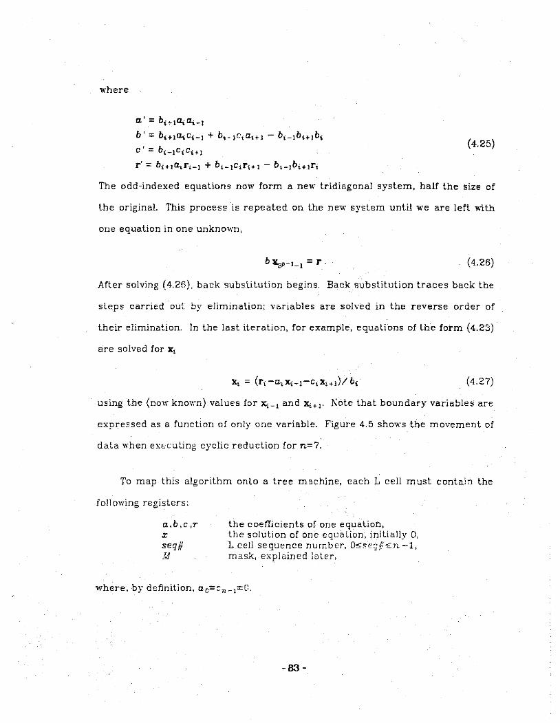
where

a'= b;+1!l;tlt-1

b' = b.,;+tD-tCi-1 + b"_lciai+l- bt-tb·i+Jbi

c' = bi-Icici+J

r' = bi+J~ri-I + bt-ICtr.~+I- bt-lbi+tri

(4.25)

The odd-indexed equations now form a new tridiagonal system, half the size of

the original. This process is repeated on the new system until we are left v.ith

one equation in one unknown,

b X,.-'-1 = r. (4.26)

After solving (4.26), back substitution begins. Back substitution traces back the

steps carried out by elimination; vo.riables are solved in the reverse order of

their elimination. In the last iteration, for example, equations of the form (4.23)

are solved for xi

(4.27)

using the (now known) values for X.-! and let+!· 1\ote that boundary variables are

expressed as a function of only one variable. Figure 4.5 shows the movement of

data when ex<Ccuting cyclic reduction for n=7.

To map this algorithm onto a tree m~chine, each L cell must contain the

following registers:

a,b ,C ,T

X

seq# M

the coefficients of one equation, the solution of one equation, initially 0, L cell sequence nurnber, O~se'jf~n -1, mask, explained later,

where, by definition, a 0=~n- 1 =0.

-83-

As Figure 4.5 shows, in each step, some L cells must send data, other L cells

must receive and process it, while still others do not participate at all. The main

problem is coordinating all this activity. We accomplish this with the use of a

mask (M), Atomic Rotate Left (ROTL.Il.), and the analogous Atomic Rotate Right

(ROTRA). The L cell's mask, computed from its sequence number, tells the L cell

whether or not it is to send information to other L cells and whether or not it is

to make use of information received from other L cells. The following algorithm

initializes 1U:

M := 1; while {mod{seq#. 2,1!)=2M-1) do!.!:= !.!+1;

where mod(i, j) is the remainder obtained after dividing i by j. Figure 4.6 shows

the sequence numbers and mask for n= 15 L cells.

Figure 4. 7 shows eight snapshots of the data communication that occurs

during cyclic reduction among n=7 L cells. The circles represent L cells; solid

circles are L cells that process data received. The arrows indicate communica-

tion. The analysis of cyclic reduction, summarized in Figure 4.5 shows that the

implementation of cyclic reduction on a tree machine requires O({log n}2) time.

Buneman Algorithm

Buzbee, Golub, and 1\ielson [BuG:\70] and Stone [Ston75] describe the Bune-

man algorithm which is similar to cyclic reduction but with the desirable pro-

perly of being stable in situations where cyclic reduction is not. Buneman's

algorithm differs from cyclic reduction in the .,;ay r is computed in (4.25) during

elimination, and tbe way xis computed in {'1.26) and {4.27) during back substitu-

tion. · During elimination, we replace the computdion for r' (4.25) with the com-

-84-

putation of two new variables d' and e '

d' = d;, + (e, - a.;d;.- 1 - c1d;,+ 1)/ b;

e' = bi+Iaiei-1 + bi-lciei+t- d'(bi+I~ci-1 + bi-I~+Ici) (4.28)

After elimination, we solve one equation in one unknown but, in place of (4.26},

we use

(4.29)

or

(4.30}

for i=2P- 1-l. During back substitution, in place of {4.27), we solve equations of

the form

(4.31)

for X;, i.e.,

(4.32)

where x,_ 1 and X.+! are now known quantities. The analysis of the Buneman alga-

rithm is summarized in Figure 4.9. This algorithm requires O({log n)2) time to

execute.

C. Iterative Methods

1. Jacobi and Jacobi Over-relaxation

The classical Jacobi algorithm transforms each equation of (4.1) into

(4.33)

(i=O, ... ,n-1) from which we obtain the iterative equation

-65-

(4.34)

{i=O, ...• n -1; k =D .... , M ). Initially, x.(o) is assigned some value, possibly the

result obtained from a direct tridiagonal linear system solver. Note that the

equations for Xc and x,_ 1 will involve two {not three) variables. For the tree algo-

rithm, as before, we assume that all information pertinent to the ith equation is

stored in£;.. For the Jacobi method, this includes the variables

coefficients of equation i

,. ... {k) x.(k) v(kl A"''. 1 l,-}t -t+l current approximation of X.. X.-!• X.+ 1

new approximation of X.

temporary.

By definition, a 0 =cn_ 1=0. Moreover, we assume that the quantities (-a.J b.},

(-c,/b;) .. and (r,lb;) are evaluated only once at the start of the operation. The

kth iteration of the Jacobi method requires two sweeps up and dmm the tree, as

shown below.

(1) l:se ROTRA to send xl~l {contained in L,_ 1) to L; which computes

(4.35)

(2) lise ROTLA to send x,:H (contained in £;.. 1) to L; which c.omputes the new

approximation for x,

(4.36)

Note that, in step 1. Lo receives x,\k) andL,._1.receives x,;• 1; these values should

be ignored by the receiving L cell. Th's is handled by the tree machine by ini-

tializing a0 and Cn-1 to 0. Iteration may continue a fL'<ed number of times or

until a criterion for convergence has been fulfilled. The stopping criterion might

-86-

be

max i xJHI) - :x;(•J i < e. i

(4.37)

for some tolerance t. After each iteration, a test. may be performed in one

sweep as described in step (3).

(3) L;. determines the value of I xj>+I) - xJ•> I and sends the result up the tree.

A T cell sends to its father the larger of the two values it receives from its

sons. The C cell compares the value it receives from its son to a pre-

assigned value for e and, depending upon the result, sends a "COKTJK"CE" or

a "HALT" signal to the L cells.

The analysis of one iteration of the Jacobi method, not including setup opera-

tions, is shown in Figure 4.10. This algorithm requires O(log n) time per itera-

lion.

The Jacobi over-relaxation (JOR) method is a generalization of the Jacobi

method. JOR replaces equation (4.34) with

x,<>+I) = (1-c.>)xl•> + c .. >[(-a.Jb;)xf~l + (-cjb,)xl~l + (r;!b,)] (4.38}

where c.> is called the relaxation factor, used to "overcorrect" or "undercorrect"

iterates produced by tbe Jacobi method. Kote that if w= 1. the equations (4.34)

and (4.38} are identical. Given that the quantities (1-w), (-c.>a;/ b,). (-we,; b;},

and (wr,/ b,) are computed before iterating, the tree algorithm for one iteration

of the JOR method proceeds as follows.

(1) Use ROTRA to send ::,'~lto L, which computes

-87-

(4.39)

(2) Use ROTLA to send x[~l to L; which computes the new approximation for X;

(4.40)

The analysis of the JOR method is shown in Figure 4.11. This algorithm requires

O(log n) time per iteration.

2. Gauss-Seidel and Successive Over-relaxation

On a sequential computer, the Gauss-Seidel method is similar to the Jacobi

method except that a new value for x, is used as soon as it is available. In place

of (4.34) ·we use

xjk+l) = (-a.,/b,)x}~i') + (-c;/b.}xftl + (r,!b;). (4.41)

which requires the value of x,C~j l) in order to evaluate x? +!). The L cells prepare

for iteration by computing and saving (-a.,!b;}, (-c,!b,). and (r;/b,). One

iteration of the tree machine algorithm is shown below.

(1) Use ROTRA to send x,. 1 to L; which computes

t, = (-c,!b,)xf!l + (r,!b.} (4.42)

This reduces (4.41) to the first-order linear recurrence

(4.43)

(2) l!se LRl to solve (4.43). L; sends up the pair (t,, -a.,_/ b.) and receives x?+I)

and xP.:..tl).

The analysis of the Gauss-Seidel method is summarized in Figure 4.12. This algo­

rithm requires O(log n) lime p:er iteration.

-88-

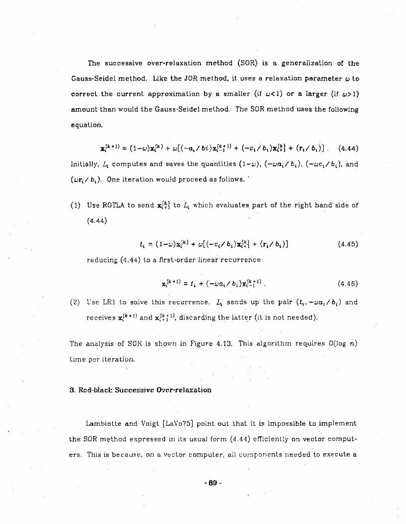
The successive over-relaxation method (SOR} is a generalization of the

Gauss-Seidel method. Like the JOR method, it uses a relaxation parameter c:.> to

correct the current approximation by a smaller (if r.>< 1) or a larger (if r.>> 1)

amount than would the Gauss-Seidel method. The SOR method uses the following

equation.

x.(k+l) = (1-w)x,Ck) + r.>[(-a.J bi)xf~t 1 > + (-'c;/ b;)xln + (r;/ b;)]. (4.44)

Initially, L; computes and saves the quantities (1-r.>), ( -c:.>aJ b,), ( -c:.>c;l b;}, and

(r.>r;/ b, }. One iteration would proceed as follows. ·

(1) Use ROTLA to send xi~! to L; which evaluates part of the right hand side of

(4.44)

(4.45)

reducing (4.44) to a first-order linear recurrence

(4.46)

(2) l:se LR1 to solve this recurrence. L; sends up the pair (t,, -c:.>a,l b,) and

receives xfk+l) and xi~j 1 >, discarding the latter (it is not needed}. . . .

The analysis of SOR is shown in Figure 4.13. This algorithm requires O(log n)

time per iteration.

3. Red-blacl: Successive Over-relaxation

Lambiotte and Voigt [LaVo75] point out that it is impossible to implement

the SOR method expressed in its usual form (4.44) efficiently on vector comput-

ers. This is because, on a vector computer, all components needed to execute a

-69-

vector instruction must be known before the instruction is executed. Equation

(4.44), however, requires that the ith component of the (k+ l)th approximation,

xjk+I), be obtained from the (i-l)th component of the (k +l)th approximation,

which is not known at the start of the vector operation. They suggest that it is

possible to reorder the equations. called a red-black ordering [Youn71], so that

a modified version of SOR can be implemented on a vector computer.

The modification amounts to separating the odd-indexed equations from the

even-indexed equations. The (k +l)th approximation of the even-indexed vari­

ables is obtained using the kth approximation of the odd-indexed variables.

Then the (k + l)th approximation of the odd-indexed variables is obtained using

the (now known) (k +l)th approximation of the even-indexed variables. I.e.,

xfk+I) = (1-:.:)xi•> + c.>[( -a, I bi)x.,(~~ + ( -c,l b.Jxl~l + (r,l b,)]

for i=O. 2, 4, .... followed by

( 4.4 7)

x}k+I) = (1-c.>)xf•l + c.>[(-r>il bi)xi~t 1 > + (-c,! b,)x{!t 1> + (r,! b.)] (4.49)

for i=1. 3, 5, .... with the equations for Xo and x,-.. 1 involving one less term.

The tree algorithm for red-black SOR is straightforward with the help of the

1 cell's sequence number (segf!) as shown below. It is similar to the JOR tree

algorithm applied to half of the set of equations each time. As before, we set

a 0 =cn-!=O and the 1 cells compute and save the values (1-c.>), (-c.>r>i/ b;),

( -c.>c,/ b;). and (c.>r;/ b,) before the start of the iteration.

(1) Vse ROTLA to send x,(n to L,. All 1 cells receive a value but only 1 cells with

even sequence numbers compute

-90-

(4.49}

(2) Use ROTRA to send xl~l to L;.. Again, all L cells receive a value but only L

cells with even sequence numbers replace their current %-approximation

v.·ith

(4.50)

(3) Use ROTLA to allow Li+I to send its current %-approximation to L;. Note

that the odd-numbered L cells will be sending x?) while the even-numbered

L cells will be sending x{k+I). Only the odd-numbered L cells will compute

t; = (1-c.J)x?l + c.J[(-c;l b;)xl~i 1 ) + (r,l b;}] (4.51)

(4) l..'se ROTRA to allow .4.- 1 to send its current %-approximation to L,. Only the

odd-numbered L cells replace their current z -approximation with

(4.52)

The analysis of red-black SOR is shown in Figure 4.14. This algorithm requires

O(log n) time per iteration.

4. Parallel Gauss: An llcrative Analog of LU Decomposition

Traub [Trau73) observed that the equations describing methods such as

Gaussian elimination, the Thomas algorithm, and LU decomposition are not

well-suited for execution on vector computers. He developed a method, called

parallel Gauss, which he compared to the Jacobi, JOR, Gauss-Seidel, and SOR

methods on a model problem run on a PDP-10 in APL.

-91-

Traub's method transforms the three equations for LU decomposition into

iterative equations. Thus, equations ( 4.11-14) are replaced by ( 4.53-56).

U;[O) = b;

uJk+!) = bo

uiH')= b,- rz;c;lu,[~/

fori=l, ... , (n-1} andk=D, ... , U-1. Letu=urm.

l; = a;/ il;-!

YJO) = r· l . '

Yc(k+l) = ro

Y _(k+!) = r - ly (k/ 1. t 1. i.-

for i=l, .... (n-1) and k=D, ... , N -1. Let y'=y(Fl.

x,ro) = ih/ U;

X (k+t)-y- 1 ,--, n-! - n-! -n-!

x/k+I) = ('[/;- c,x,ft{)lu,

for i=(n-2), ... , 0 and k=O, ... , P-1. Let x=x(P)_

(4.53)

(4.54}

(4.55)

(4.56)

For each of the iterative equations (4.53, 4.55 and 4.56), Traub noted that

after the jth iteration, u,fil, y/il, and x,Ul, are correct for i,;j + 1. This means

that each iteration requires at most (n~l) iterations. This presents a savings

. for \'ector computers since these components need not be recomputed, i.e. the

len,;lh of the vector processed decreases by one in each iteration.

The tree algorithm for Traub's method is sho,·n below.

(1) Compute u,. L, initia!iz2s u,=b,. In the kth iteration, use ROTRA to send

U;(~/ to L;. which computes (4.53). Iterate M times, i.e., until convergence

- B2-

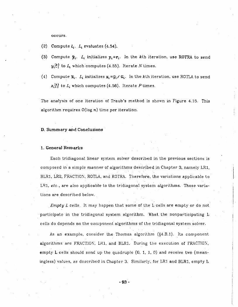
occurs.

(2) Compute l;. L; evaluates (4.54).

(3) Compute Yt· L; initializes Y; =r,. Jn the kth iteration, use ROTRA to send

y,'!:/ to L, which computes (4.55). lterate N times.

(4) Compute x,. L; initializes x,=y;/fi;. Jn the kth iteration, use ROTLA to send

x/-i'/ to L; which computes (4.56). Jterate P times.

The analysis of one iteration of Traub's method is shown in Figure 4.15. This

algorithm requires O(log n) time per iteration.

D. Summary and Conclusions

1. General Remarks

Each tridiagonal linear system solver described in the previous sections is

composed in a simple manner of algorithms desc.ribed in Chapter 3, namely LR1,

B1R1, 1R2, FRA.CTJO};, ROT1A, and ROTRA. Therefore, the variations applicable to

LR1, etc., are also applicable to the tridiagonal system algorithms. These varia·

tions are described below.

Empty L cells. lt may happen that some of the 1 cells are empty or do not

participate in the tridiagonal system algorithm. What the nonparticipating 1

cells do depends on the component algorithms of the tridiagonal system solver.

As an example, consider the Thomas algorithm (§4.B.1). lts component

algorithms are FRACTJOJ\, 1Rl. and B1Rl. During tbe execution of FRACTJO:\,

empty 1 cells should send up tbe quadruple (0, 1, 1, 0) and receive two (mean­

ingless) values, as described in Chapter 3. Similarly, for 1R1 and B1R1, empty 1

-93-

cells should send up the pair (0, 1) and receive two values. In short, it is not

necessary to make any modification to the component algorithms in order to

use them in the implementation of the Thomas algorithm or of any of the other

tridiagonal system solvers.

Solving several independent tridia.gona.l linea.r systems simultaneously

us·ing a. direct method. It is possible to solve more than one tridiagonal linear

system simultaneously, provided that there are enough 1 cells to accommodate

all of the systems, with one equation occupying one 1 cell, and all systems are

solved by the same method. An immediate concern are the boundaries between

different systems. We find, however, that if the coefficients of the boundary

equations are properly initialized, the algorithms execute correctly.

As an example, consider the melhod of 1U decomposition (§4.B.2, equations

( 4.10-15)) simultaneously applied to two tridiagonal linear systems. Recall that

each 1 cell contains the following variables:

a,b,c,r l,u,y X

coefficients of one equation storage for intermediate values solution of one equation

where, by definition, a.0= Cn _ 1 =0. For the convenience of the reader, we repeat

equations (4.10), (4.12), and (4.13) here.

[ 1 0 1 [ u 0 co 0

ll 1 ul cl

A'= LU = lz 1 ( 4. 1 0)

Un-2 Cn -2

0 ln -l 1 0 Un-l

where

-94-

and

up = bo

U; = -a.i ci-1 + biui-1

0 + lu1_ 1 i=1,2, .... n-1

(4.12)

i=1,2, ... ,n-1 (4.13)

which expresses U; as a quotient of two linear functions of U;- 1• and l, as a func-

tion of Uj. The component algorithms of LU decomposition are ROTRA, FRAC-

TJON. LR1, and BLRL Figure 4.16 shows the L cells which contain the two linear

systems. Let L; represent the L cell with sequence number i. The first system

is stored in cells Lc through Ln_ 1; the second is stored in L,. through Ln+m-J·

The first step uses ROTRA to send c,_, (stored in the {i-l)th L cell) to the

ith L cell. This causes L 0 and Ln to receive Cn+m-l and Cn-l respectively. Note,

ho\\·ever, that a 0 a!1d Un will be multiplied with Cn+m-I and cn-l in the next step,

and that all four terms are 0.

The second step uses FR<\CTlO\ to evaluate equation (4.12). Each L cell

must send up the quadruple { -a,c,_1, b,, D. 1). L 0 and L, have the added condi-

tion that the first component, i.e. -a.,c,_ 1, must be D. We see that this condition

is satisfied as a 0 , cn+m-I• Un, and cn-l are all D. FR<\CTJON, therefore, executes

correctly.

The third step is for each L cell to compute l, using equation (4.13). The

cells Lc and L, must have l 0 and ln equal to D. This is, in fact, the case because

a 0 and Un are both D.

Thi; continues through the rest of the algorith:n. The algorithm does not

need to make a special cas2 of the boundary L cells because the proper initiali-

zation to 0 of some of the!r co3tTici2~ts a£~U!e~ ~h2 correct evaluation of other

values.

-95-

Solving several independent trid1:a:;onal linear systems simultaneously

using an iterative method. It is also possible to solve several systems simultane·

ously with an iterative method. As with a direct method, the potential problem

of error occurring in the boundary L cells is avoided by proper initialization of

the boundary coefficients. The number of iterations needed to solve all of the

systems is the maximum number needed to solve any one of the systems, i.e., it

will take as long to solve all of the systems as the least convergent of the sys·

terns.

Solving-the same system for different constant values. The LU decomposi·

lion, LU decomposition variant, and recursive doubling methods allow the user

to solve the same tridiagonal system for diflerent values without having to

decompose the coefficient matrix each lime. The implementation is straightfor·

ward.

The coefficient matrix is decomposed once at the start of the operation.

One set of constants is stored in the L cells and the algorithms LRl and BLRl are

executed. The solution values are flushed out, a new set of constants is read in,

and the tree is ready to execute 1.'< 1 and BLRl once again. This continues as

many times as there are sets of constants.

2. Comp.:.riso;:: o~ lhc Tree A:gorithms

Figure 4.17 shoves a summary of the complexity of the direct tridiagonal

system solvers. All methods except cyclic reduction and the Buneman algo·

rilhm require O(log n) time. Although cyclic reduction and the Buneman algo·

rithm execute O(log n) arithmetic operations, communication requires O((log

n) 2) time. The increased communication tinoe could be acceptable if it were

. 9S.

offset by a significant reduction in the number of arithmetic operations. As this

is not the case, neither cyclic reduction nor the Buneman algorithm can com­

pete with the other, more traditional, algorithms.

Of the remaining, the LU decomposition variant is the least desirable. It

requires at least 60% more parallel additions, 25% more parallel multiplications,

and 10% more communication lime than the Thomas algorithm, Gaussian elimi­

nation, LU decomposition, or recursive doubling variant. This is because of its

use of LR2 which, as has been pointed out in Chapter 3, is considerably more

expensive than LR1 and somewhat more expensive than FRACTJON.

The three traditional tridiagonal linear system solvers and recursive dou­

bling emerge as the best, with the Thomas algorithm ho!Uing a slight communi­

calion time edge over Gaussian elimination and LU decomposition. LU decompo­

sition, of course, is to be preferred if one must solve many different linear sys­

tems using the same coefficient matrix.

Comparing the iterative methods (Figure 4.18) is more difficult as the rate

of convergence of the methods must also be considered. Considering only arith­

metic operations and communication time per iteration, the Gauss-Seidel and

SOR methods compare poorly with the Jacobi and JOR methods. However, the

Gauss-Seidel method has a rate of convergence approximately twice that of the

Jacobi method [Arnes77], provided both converge. For the particular case of

solving Laplace's equation on a square region, if h is the space between grid

points (see Figure 2.1), Ames sho.vs that computation time is reduced by the

factor 2h-1 if one uses SOR rather than the Gauss-Seidel method. However, one

must consider the overhead of obtaining the optimum relaxation factor c.> before

deciding to use SOR over Gauss-Seidel. The parallel Gauss method described by

Traub has the least amount of computation per iteration. However, one must

-97-

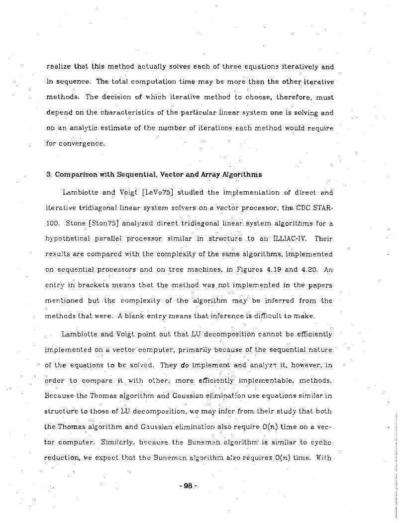
realize that this method actually solves each of three equations iteratively and

in sequence. The total computation time may be more than the other iterative

methods. The decision of which iterative method to choose, therefore, must

depend on the characteristics of the particular linear system one is solving and

on an analytic estimate of the number of iterations each method would require

for convergence.

3. Comparison with Sequential, Vector and Array Algorithms

Lambiotte and Voigt [LaVo75] studied the implementation of direct and

iterative tridiagonal linear system solvers on a Yector processor, the CDC STAR-

100. Stone [Ston75] analyzed direct tridiagonal linear. system algorithms for a

hypothetical parallel processor similar in structure to an ILLJAC-IV. Their

results are compared with the complexity of the same algorithms, implemented

on sequential processors and on tree machines, in Figures 4.19 and 4.20. An

entry in brackets means that the method was not implemented in the papers

mentioned but the complexity of the algorithm may be inferred from the

methods that were. A blank entry means that inference is difficult to make;

Lambiotte and Voigt point out that LU decomposition cannot be efficiently

implemented on a vector computer, primarily because of the sequential nature

of the equations to be sol·;ed. They do implement and analyz~ it, however, in

order to compare il. wilh other, more efficiently implernentable, methods.

Because the Thomas algorithm and Gaussian elimination use equations similar in

structure to those of LU decomposition, we may infer from their study that both

the Thomas algorithm and G"ussian elimination also require O(n) time on a vec­

tor computer. Similerly, b'2cause the Bunemo.n algorithm is similar to cyclic

reduction, we expecl that the Bunem.~n algorithm also requires O(n) time. With

-98-

this in mind, we see from Figure 4.19 that tree machines consistently do better

(asymptotically) than either sequential or vector processors.

Stone asserts, for reasons similar to Lambiotte and Voigt's, that conven­

tional tridiagonal linear system solvers cannot do better than O(n) time on an

array processor. Consequently, he does not present an implementation of either

the Thomas algorithm, Gaussian elimination, or LU decomposition in his paper.

lf his premise is correct, we see from Figure 4.19 that, except for cyclic reduc­

tion or the Buneman algorithm, tree machines match or better the complexity

of algorithms run on array processors. Recall that for cyclic reduction and the

Buneman algorithm, tree machines required O(log n) arithmetic operations and

O((log n)2) communication time. Stone's analysis considered only arithmetic

operations ar.d did not take into account costs of data routing, arrangement,

and rearrangement, which may make his estimates unrealistically low.

Lambiotte and Voigt also analyzed three iterative methods, the Jacobi

method, red-black successive over-relaxation, and Traub's parallel Gauss algo­

rithm. They conclude that methods such as the Gauss-Seidel method and suc­

cessive over-relaxation are not efficient on a vector computer because of the

sequential nature of the equations in,·o]\·ed. Figure 4.20 compares the orders of

complexity of six different iterative methods when implemented on sequential,

vector, and tree processors and it shows that tree machines produce con­

sistently better results.

- C<)-

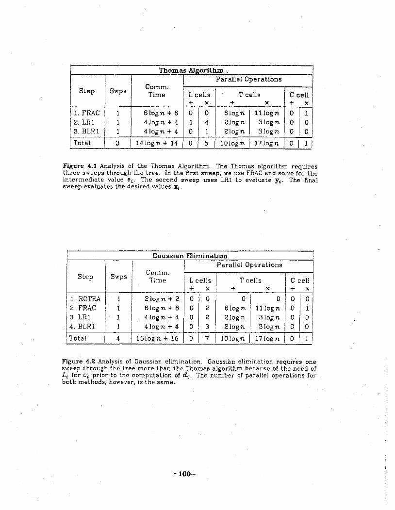
Thomas Algorithm Parallel Operations

Step Swps Comm. Time L cells T cells C cell

+ X + X + X

1. FRAC 1 6logn + 6 0 0 6logn 11logn 0 1 2. LR1

I 1 4logn + 4 1 4 2logn 3logn 0 0

3.BLR1 1 4logn + 4 0 1 2logn 3logn 0 0

Total 3 14!ogn+ 14 0 5 lOlogn I 17log n 0 1 I

Figure 4.1 Analysis of the Thomas Algorithm. The Thomas algorithm requires three sweeps through the tree. In the first sweep, we use FRAC and solve for the ir.termediate value e;. The second sweep uses LRl to evaluate Yi· The final sweep evaluates the desired values J!i.

Gaussian Elimination !

I Parallel Operations I Step Swps

Comm.

I C cell I I Time L cells T cells

I + X + X + X

1

1. ROTRA 1 2logn + 2 0 0 0 : 0 0 I ~I 2.FRAC 1 6logn + 6 0 2 B!ogn 11log n 0

13.LR1 1 4logn + 4 0 2 2logn 31ogn 0 01 /4.BLR1 1 I 4logn + 4 0 3 2logn 3logn 0 ol

I ' I Total 4 16logn + 16 I 0 7

I lOlogn I 17log n I 0 I 1 i I

Figure 4.2 Analysis of Gacssiar. elimir..ation. Gaussian elimir:ation requir.es one sweep throt:.gl: the tree more than U:e T.hor.1as algorithm becat:se of the need of L; fer c; prior to tl:e computation of d;. The r:umber of parallel operatior:s for boll: metl:ods, l:owever, is the same.

-100-

LU Decomposition Parallel Operations

Step Swps Comm. Time Lcells T cells C cell

+ X + X + X

1. ROTRA 1 21ogn + 2 0 0 0 0 0 0 2.FRAC 1 61ogn + 6 0 2 6logn 11logn 0 1 3. 0 0 0 1 0 0 0 0 4.LR1 1 4logn + 4 0 1 2logn 3log n 0 0 5. BLR1 1 I 4log n + 4 0 3 2logn I 3logn 0 0

' Total 4 161ogn + 16 0 7 I lO!ogn f17logn I 0 1

Figure 4.3 Analysis of LU decomposition. We need four sweeps through the tree machine. The first sweep sends c1_ 1 to L,. The second sweep uses FRACto obtain the u,. Note that after the second sweep, L; has received both U; and U.-l· It can immediately compute l,=a..Jui-l· The tl-Jrd sweep (step 4) computes the intermediate values y,. The f.nal sweep gives the desired values x,.

LU Decomposition Variant Parallel Operations

Step Swps Comm. Time L cells T cells C cell

i + X + X + X

1. ROTRA 1 I 2logn + 2 0 0 o I o 0 Ol 2.LR2 1 I 10logn+ 10 0 2 12logn [ 16logn 0 01 3. 0

I 0 0 2 0 ' 0 0

01 4. LRl 1 41ogn + 4 0 1 2logn

I 3logn 0

! 0,

5. BLR1 1 I 41ogn + 4 0 3 2logn ' 3logn 0 0

Total I 4 : 201ogn+20 I 0 B 16logn I 22log n ! 0 I 0 !

Figure 4.4a Analysis of LU decomposition variant. After the two first sweeps (Steps 1·2), g, has been determined. Step 3 ccmp>.:les u, arod !;. Steps 4 and 5 are similar to Steps 4- ar:d 5 cf LU deco:r.1positicr:.

-101-

Poo Pu p22 Pss p44 P,5 Faa p?? X Poo Pu p22 Psa p44 p55 Faa

I== Poo Pot P12 P2s Ps4 p45 P5a Pa? X Poo Pot pl2 p23 Ps4 p45

F= Poo Pot Po2 Pos Pt4 p25 Psa p4? X Poo Pot Po2 Poa

F= Poo Pot Po2 Pos Po4 Po5 Poa Po?

Figure 4.4b Recursive doubling for n=B, where P;; = n P,. In log n = 3 steps, k=i

the desired products P.,, 0Sis7 are obtained.

Recursive Doubling Variant

Step

1. ROTRA 2.LR1M 3.

4.LR1 5. BLR1

Total

Swps

1 1 0

1

1

I 4

Comm. Time

2logn + 2 Blogn + 8

0 4logn + 4 4logn + 4

L cells + X

0 0 0 0 0

0 2 2 1

3

18logn+ 18 0 8

Parallel Operations

T cells + X

0 Blogn

0

2logn [ 2logn

0 12log n

0

3logn 3logn

C cell + X I

0 0 0 0 0

0 0 0

0 0

lOlogn i lBlogn 0 0

Figure 4.4c Ar:alysis of recursive dm.:bling variant. LR!M is a modified versior: of LRl in w~Jch the coefficient of the recurrer:ce is a (2 x 2) r:Jatrix, the variables are 2-vectors, and the reccrrence equation has no constant term. Consequently, the T cells r:Just perform one matrix multiplication during the upward sweep and one matrix-vector multiplication dcring the downward sweep.

-102-

o; 0 0 0 ro• 1' 1 1* r~. ;) 2 (h { ~.)

r~~ 3*

(~. 4 ~.l (~~ 5 5* ~ ~.} 6 6 6 (a) (b) (c) (d) (e)

Figure 4.5 Data communication in cyclic reduction. Elimination takes place in (a) and (b) while back scbstituticn takes place in (d) and {e). The numbers represent equations. An arrow rneans that the coeft'iclents of one equation are required by (and sent to) another. A prime (') means that ar: equation has beer: elimir:ated. A star (•) means that the equation has been solved. ln (a), equation i {i=l,3,5) receives the coefficients of equations (i-1) and (i+l); equation i is modif.ed, eliminating the even-indexed variables. In (b) the step is repeated with only equations 1, 3, and 5 participating. In (c), equation 3 has become an equa­tion in one variable {i.e., x3). We solve for X3. In (d), the value of X3 is sent to (the modified) equations 1 and 5 which are now able to solve for X1 and JCs respec­tively. In (e), the rest of the variables are evaluated.

i Sequence#: I Mas~:

0 1 1 2

2 3 4 1 3 1

5 2

6 1

7 B 4 1

9 2

10 1

Figure 4.6 L cell sequence r:umbers ar:d I:Jask.

-103-

11 3

12 1

13 2

14 ', 1 I

(a} ROTRA .,. ' a,..........e__,.a_... •---a--.. •-a

(b) ROTLA r a a-•-a_....e....--a-e-a

(c) ROTRA a g;--- a ...... --- a ... -a a (d) ROTLA a c~ • .,... a ~ a (e) ROTRA a ~0 a .............. • a (f) ROTLA a r;

1111 a ..... a .. a --"\ a (g) ROTRA

r: . •-a--•-a--e-a--..•

(h) ROTLA •-a-•-a-•-a.--.e

Seq# 0 1 2 3 4 5 6 Mask 1 2 1 3 1 2 1

Figure 4. 7 Communication among the L cells during cyclic redt:ction for n=7. In tl::e f.rst elimination step, the even-indexed L cells must send tl::eir coe:Eicients to tl::e odd-indexed L cells. To do this, we t:se ROTRA (a) and ROTLA (b). In both figures, L cells with /.P--1 are programmed tc ser.d and receive ir:formatior., but only L cells with M> I (solid circles) are programmed to process tl:e ir:fcrr:1ation. II: general, dt:ring the ith elimination step, (i=1,2, ... ,log(n-1)-l), L cells with /.P--i send ar:d receive information while only L cells wit!: M>i process it. (c) ar:d (d) show the movement of data during tl::e second elimir.ation step. In the it!:: back sc:bstitution step, (i=log(n+l)-1, ... ,1), L cells will:: .M?:i ser:d and receive infori:la­ticn while orJy those with M=i process it. (e) throc:gl: (I:) sl:ow tl:e movemer:t of data during back substitc:tion.

-104-

Cyclic Reduction Parallel Operations

Oper-Swps

Comm. ation Time L cells T cells C cell

+ X + X + X

Elimin Z(h-1) 2(h-1)(2h+5) 4(h-1) 16(h-1) 0 0 0 0 I Solve 0 0 0 1 0 0 0

~I I Backsub Z(h-1) 2(h-1)(2h+5) Z(h-1) 3(h-1) 0 0 0

al 4(h-1) ! 4(h-1)(2h+5) 6(h-1) 19(h-1)+ 1 0 0 0 0

Figure 4.8 Analysis of cyclic reduction, h=!og(n ... l). Both elimination and back substitution require (h-1) iterations and each iteration involves one RDTRA and one RDTLA; hence, each reqLires 2(h-1) up and down sweeps through the tree. In one execution of RDTRA (or RD-::'LA), all cells send 4 atoms to their fathers during the upward sweep and 4 atoms to their sons durir.g the downward sweep. Pipelin­ing allows aT cell to send data from its son (father) to its father (son) as soon as the data is received. With pipelining. one execution of R07RA requires 2h"'5 com­munication steps. As elimination and back substitution each take 2(1!.-1) sweeps, a total of 4(h.-1)(2h.•5) communication steps are required. Only the L cells exe­cute any arithmetic instructions. During elimination, selected L cells solve for a', b', c', r', as found in equatior: ( 4.22), after every 2 sweeps. After elimination, one L cell executes one division (4.23). During back substitution, selected L cells evaluate (4.24). The entire operation requires D(h.2)=D((Iog n)2) time.

Buneman Algorithm Parallel Operations

.

Oper- Comm. ation

Swps Time L cells T cells C cell

+ X + X +

Eli min Z(h-1) 2(h-1)(2h+5) B(h-1) 20(h-1) 0 0 0 Solve 0 0 1 1 0 0 0 Backsub Z(h-1) 2(h-1)(2h+5) 3(h-1) 3(h-1) 0 0 0

Total I 4(h-1) 1 4(h-1)(2h+5) I 11(h-1)+1 23(h-1)+ 1 0 0 0

Figure 4.9 Analysis of the Bunemar. algorithm, h.=log{n+l). The stability p~o,·!d­ed by this algorithm (compared to cyclic reduction) cor:Jes at the cost of added parallel additions and multip!Jcations.

-105-

X

0

0

0

0

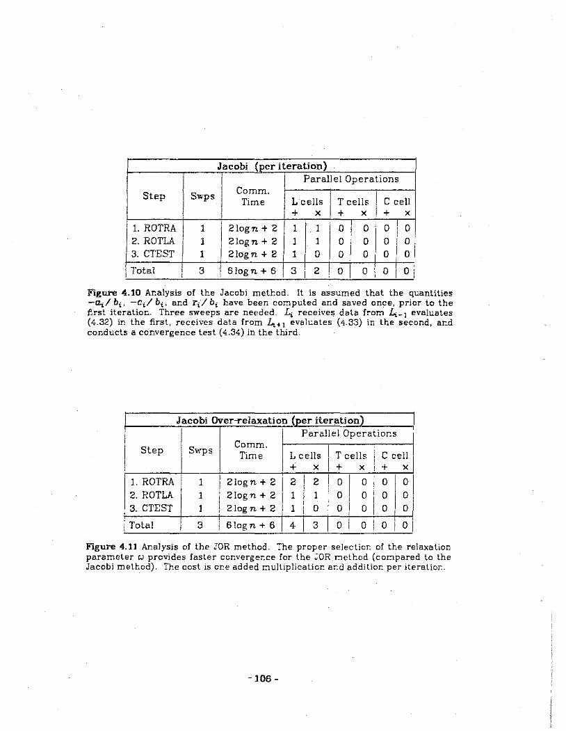
Jacobi (per iteration) Parallel Operations

Step Swps Comm. Time L cells T cells C cell

' + X + X + X

1. ROTRA 1 I 2logn + 2 1 1 0 0 I D 0 2. ROTLA 1 2logn + 2 1 1 D 0 0 0 3. CTEST 1 2logn + 2 1 0 0 0 0 0

\Total 3 ! 6logn + 6 3 2 0 I 0 i 0 I o I I !

Figure 4.10 Analysis of the Jacobi method. It is asstomed that the quantities -a;, I b;. -C;/ b;, and r;/ b; have been computed and saved once, prior to the first iteration. Three sweeps are needed. Li receives data from 4-1 evaluates (4.32) in the first, receives data from 4+ 1 evah.:ates (4.33) in the second, and conducts a convergence test (4.34) in the third.

Jacobi Over-relaxation (per iteration) Parallel Operations

Step Swps Comm.

I Time L cells T cells C cell I I + X I + X + X

1. ROTRA 1

I 2log n + 2 I 2 2

D I 0 I D I D I 2. ROTLA 1 2logn + 2

I 1 1 D I 0 I o I o.

3. CTEST 1 I 2logn + 2 1 0 o I D 0 i 0

I I 6log n + 6 I o I 0 I 0 I ' 1 Total 3 4 3 Ol

Figure 4.11 Analysis of the JOR method. The proper selectim: of the relaxation parameter c.; provides faster convergence for the .;oR neU:od (col:lpared to the Jacobi method). The cost is or:e added multiplication ar.d additior. per iteratior..

-106-

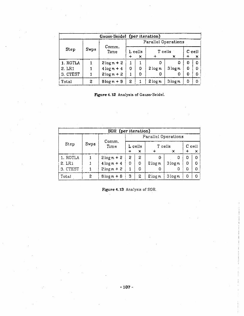
Gauss-Seidel (per iteration) Parallel Operations

Step Swps Comm. Time L cells T cells C cell

+ X + X + X

1. ROTLA 1 2logn + 2 1 1 0 0 0 0 2. LR1 1 4logn+4 0 0 2logn 3logn 0 0 3. CTEST 1 2logn + 2 1 0 0 0 0 I 0

1 Total 2 I 81ogn + 8 2 1 I 2logn 3logn 0 0

Figure 4.12 Analysis of Gauss-Seidel.

SOR (per iteration) Parallel Operations I

Step Swps Comm.

I Time L cells T cells C cell

' + X + X + X

' 1. ROTLA 1 2logn + 2 2 2 0 0 0 0 . 2. LRl 1 4logn + 4 0 0 2logn 3logn 0 0 13. CTEST j 1 2logn + 2 1 0 0 0 0 0.

Total I 2 J Blogn + 8 I 3 I 2 2logn ' 3logn 0 I ol !

Figure 4.13 Analysis of SOR.

-107-

Red-Black SOR (per iteration) Parallel Operations

Step Swps Comm.

Time 1 cells T cells C cell + X + X + X

1. ROTRA 1 2logn + 2 2 2 0 0 0 0 2.ROTLA 1 2logn + 2 1 1 0 0 0 0 3. ROTRA 1 2logn+ 2 2 2 0 0 0 0 4. ROTLA 1 2logn + 2 1 1 0 0 0 0 5. CTEST 1 I 2log n + 2 1 I 0 0 0 0 0

Total 5 10logn+10 I 7 6 0 0 I 0 I 0

Figure 4.14 Analysis of red-black SOR.

Parallel Gauss (per iteration) I Parallel Operations

Step Swps Comm. Time 1 cells T cells C cell

+ X + X + X

1. ROTRA 1 2logn + 2 1 1 I

0 0 0 I

0' CTEST 1 2logn + 2 1 0 0 0 0 0

2. 0 0 0 1 0 0 0 01

3.ROTRA 1 2logn + 2 1 1 0 0 0 I o, CTEST 1 2logn + 2 1 0 0 I 0 0

I 0

I I

4. ROTLA 1 2logn + 2 1 1 I 0 I 0 0 I ~I CTEST 1 2logn+ 2 1 0 I 0 I 0 0

Figure 4.15 Analysis of Parallel Gat:ss.

-108-

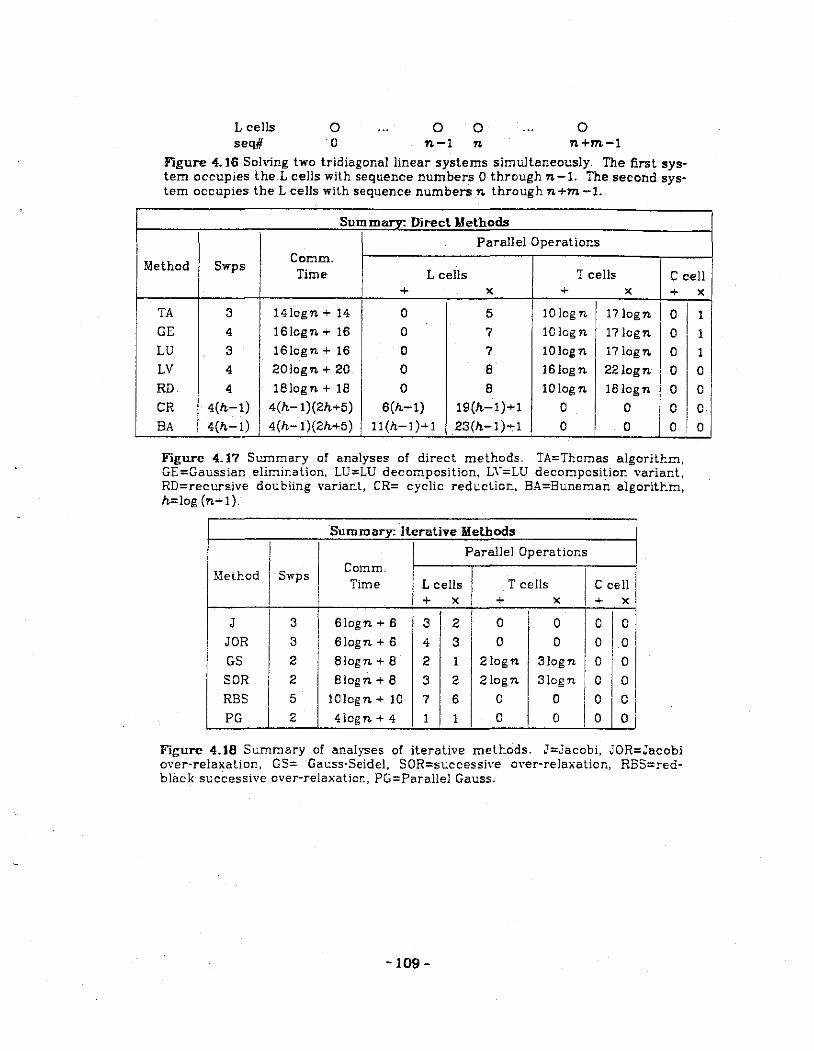
L cells seq#

0 0

0 0 n-1 n

0 n+m-1

Figure 4.16 Solvlng two tridiagonal linear systems simultaneously. The first sys­tem occupies the L cells with sequence numbers 0 through n-1. The second sys­tem occupies the L cells with sequence numbers n through n+m-1.

Summary: Direct Methods

Parallel Operations

Method Comm.

Swps Time L cells T cells C cell

+ X + X +

TA 3 14logn + 14 0 5 !Ologn I 17logn I 0 GE 4 16logn + 16 0 7 10 log n 17logn 0 LU 3 16logn + 16 0 7 10 log n 17logn 0 LV 4 201ogn + 20 0 8 16log n 221ogn 0 RD 4 1Biogn + 18 0 8 10 log n 18logn 0

CR 4(h-1) 4(h-1)(2h+5) 6(h-1) 19(h-1)+1 0 0 0

BA 4(h-1) 4(h-1)(2h+5) 11(h-l)~l 23(h-1)+1 0 0 0

Figure 4.17 Summary of analyses of direct methods. TA=Thomas algorithm, GE=Gaussian elim.ir:ation, LU=LU decomposition, LY=LU decoT!'lpositio:r.. variant, RD=recursive dot:bling variant, CR= cyclic reduction, BA=Buneman algoritr.m, h=log (n+1).

Summary: Iterative Methods

Parallel Operatior:s

Method Swps Comm.

I Time L cells T cells C cell

+ X + X + X

J 3 6logn+6 3 2 0 0 0 0

JOR 3 61ogn + 6 4 3 0 0 0 0

GS 2 81ogn + 8 2 I 2logn 31ogn ' 0 0

SOR 2 Blogn + 8 3 2 2logn 31ogn I o I o RBS 5 1Clogn + 10 7 6 0 0 I 0 I 01 PG 2 4lcgn + 4 1 1 0 0 ! 0 0

Figure 4.18 Summary of analyses of iterative metr.ods. J=Jaccbi, JOR=Jacobi O\'er-relaxatior.., GS= Gat:.ss-Seidel, SOR=sw.ccessiYe over-relaxation, RBS=red­black successive over-relaxaticr:, PG=Parallel Gauss.

-109-

X

I 1

1

1

0

0

I 0

I 0

~Melbocb '

·Method AJaorU~ Comple~it~

seauential· Veotor· Arrey Tree' .. . ;·

c'ftJ ' > ' '

TA " Joe" GE " [n] loc n LU " " log n LV " [n] leg n RD n logn in log n loan ·loan CR n n. log n (loan)' BA I n [n] loan (k>l n)2

r

Figure 4.l9 Comparison of the ordets of ~ymptotic complexity of direct tridiag­onal linear system solvers for sequential, vector, ~rray, and tree processors. TA=Thpmas algorithm, GE=Gaussian elimination, LU=LU decompo,iUon, LV=LU decomposition variant, RD=recursive. doublina. Cllaeyclic reduction;' BA=Buneman algorithm. The. results f()r vector proc,esaqr.a 1fere. desoribed by Lar:1biotte and Voigt [LaVo75]. Entries in· brackets indicate that the methods were not implemented· by Lambiotte and Voilt but ttl• camplexity of the algo­rithms can be inferred from the results obtained from methods that were. The rest;lts for array p.roeessors were described by Stone [5ton75). Bhank e~tries mean that imPlemttntaUons of these meth.cts have not been described in tb:e literature. ·

lter.Uve llelh-

Method t Ale:orithm Complexity {Iter iteration)

Sequential Vector Tree

J n' n Joan JOR n [n] locn GS n (n] loan

SOR n lnl ' loan RBS " " log n PG " " logn

fi&ure 4.20 Comparison Of the orders of asymptotic complexity of iterative tr~di­agonal linear system solvers for sequential, vector, an4 tree . pJ"ocessort. J=~acobi, JOR=Jacobi over-relaxation, GS=Gauss·Seidel, SOR=successive over· relaxation, RBS=red·black successh•e over-relaxation, PG=Parallel Gauss. The results for vector processors were described by Lar:1biotte ar.d Voigt [LaVo75). Entries in brackets indicate ir.ferred orders of complexity (see caplior. or Fiaure 4.19).

-110-

";J I

•

..

A. Overview

) ~-:

Tbe primary Gbj_ective of this dissertation is t.he patallel,solution on· a t;ree

machine of Laplace's equation

(5.1)

. or Po_isson's equation

o~z li~z - 2 + - 2 =r, r a constant 8z ay ' ... (5.2)

on a rectangular region. ·The valueB.of lhe function z. are known on the boundary

oLthe region and the object is to obtain an approximation of z at any point in

the interior .. The method of finite dift'erences lays a rectangular mesh with n

rows and m.. :e;:olumns on the region. Equation (5~1) or (5.2) is then replaced by

(n-2) x{m-:""2) secc:md-order·difference equations, one for each interior mesh

point. The solution oU.he system of. ditJerence equations pro'\tides an approxima ..

tion of z at each of the mesh points. The system of equations is block ..

tridiagonal and may be solved by iterative or direct numerical methods. Figure

5. f sho,\·s a me~fi vdtb ~,.;_·=7 ~rid m. =9. The. m~sh points, both boundary and inte­

rtof, are 'number'ed from from 0 through '(;._m ~1) in ro~ rita)or order. The - ~. ~- ': ~: ~ ~ .. ·, ·.. . ~ '·- ' '· ~ '- ~- ~ . { ~ '. -:· ' . : . . ; -. . ; :. "

' c'ott~spohairig' block-tridiagonal sysfem or equations is showri in Figure 5.2.

:1'

The iterative methods for solving block-tridiagonal linear systems con­

sidered in this chapter are point iterative methods, block iterative methods, and

alternating direction implicit methods. Point iterative methods modify the

value of one interior mesh point at a time. These methods are called explicit

methods because the new value at a mesh point is explicitly expressed as a func­

tion of already computed approximations of neighboring points. Examples are

the Jacobi, Jacobi over-relaxation (JOR), Gauss-Seidel, and successive over­

relaxation methods (SOR) methods [Youn71, Ames??]. Another class of iterative

methods are block iterative methods (also called methods by lines). At each

step, the values of one or more rows of points are modified, typically involving

the solution of a tridiagonal system of equations. Such methods are called

implicit methods because the approximate value of a mesh point is expressed as

a component of the solution of a linear system. These methods have been exten­

sively studied [Ames??, DoRa56, FoWaBO, Hell??, Hel17B, PeRa55, Varg62,

Youn71]. Examples are Jacobi by lines, Jacobi over-relaxation by lines, Gauss­

Seidel by lines, and SOR by lines. A third class of methods are alternating direc­

tion implicit (AD!) methods [PeRa55, DoRa56], which first improve the values of

points a row at a time and then a column at a time. As with block iterative

methods, the solution of a row or column of points requires the solution of a tri­

diagonal linear system. This chapter presents tree implementations of these

three classes of algorithms.

Direct methods for the solution of sparse block-tridiagonal systems have

also been widely studied. The initial paper by Eockney [Eock65] described a

method based on Fourier transform and cyclic reduction and required O(n3)

arithmetic operations compared with O(n 4 ) operations required by traditional

band matrix methods. A stable version of cyclic reduction was described and

- 112-

implemented in FORTRAN by Buneman [Bune69]. A further improvement was

made using the Fast Fourier Transform [BuGN70]. Subsequent work includes

studies of non-rectangular regions [BDGG71, DiFe76, Swar74, SwSw73, Swee73].

Heller [Hell76, nell77] describes still another variation of cyclic reduction and a

general analysis of direct block-elimination methods. Generalized cyclic reduc­

tion techniques are described by Sweet [Swee74] and Hageman and Varga

[HaVa64]. Other direct methods include an LU decomposition of block­

tridiagonal systems described by Varah [Vara72] and a decomposition based on

the computation of the eigenvalues of the coe!Iicient matrix described by Buz­

bee [Buzb75]. Survey papers have been written by Dorr [Dorr70] and Heller

[Ee117B].

1 attempted to develop a tree machine algorithm to implement the Bune­

man version of cyclic reduction as described by Buzbee, Golub, and Nielson

[BuG:\70]. Unfortunately, the best algorithm 1 found was much more complex

than the algorithms required to solve the block-tridiagonal system using tradi­

tional iterative methods. As a result, I have not included cyclic reduction in this

dissertation.

B. Point iterative Methods

Approximating an elliptic partial differential equation (pde) on a rectangu­

lar region using finite differences involves (1) laying a rectangular mesh of

points over the region (Figure 5.1), (2) assigning a value, known a priori, to each

boundary point, (3) replacing the elliptic pde with a system of linear difference

equations, and (4) sol•·ing the resulting linear system. The boundary values

(conditions) remain fixed throughout the process and determine the solution for

-113-

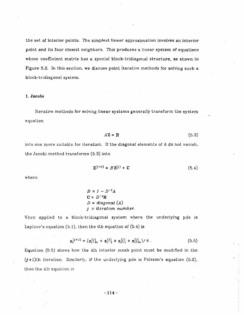
the set of interior points. The simplest linear approximation involves an interior

point and its four closest neighbors. This produces a linear system of equations

whose coefficient matrix has a special block-tridiagonal structure, as shown in

Figure 5.2. Jn this section, we discuss point iterative methods for solving such a

block-tridiagonal system.

1. Jacobi

Iterative methods for solving linear systems generally transform the system

equation

AZ= R (5.3)

into one more suitable for iteration. If the diagonal elements of A do not vanish,

the Jacobi method transforms (5.3) into

where

B =I- D- 1A

c = n-'R D = diagonal (A) j = iteration number.

(5.4)

When applied to a block-tridiagonal system where the underlying pde is

Laplace's equation (5.1), then the ith equation of (5.4) is

Z (i+I) = (z(il + zUl1 + z(il1 + zUl )/4 o. o.-m o.- .. + 1-+m · (5.5)

Equation (5.5) shows how the ith interior mesh point must be modified in the

(j +1)th iteration. Similarly, if the underlying pde is Poisson's equation (5.2),

then the ilh equoLion is

- 114-

(5.6)

where his the uniform distance between two adjacent mesh points.

After an initial value is assigned to each z-variable, equation (5.5) or (5.6) is

used to obtain new iterates. Equations (5.5) and (5.6) are true even for interior

points adjacent to the boundary; such points would have boundary points as one

or more of their neighbors. The (j+ l)th approximation of an interior point is

determined entirely by the jth approximation of it.s four neighbors. This charac-

teristic of the Jacobi method allows parallelism to be introduced: it is theoreti-

cally possible to modify all interior points simultaneously.

To implement this method on a tree machine, we distribute the mesh points

(both boundary and interior) among the L cells. one. to an L cell and in row-

major order. Each L cell holds the following registers

z

mask t

the current value of one boundary or interior point (boundary points never change their values), "0" if boundary point, "1" if interior point, temporary, serves as an accumulator.

Boundary points are distinguished from interior points by a mask in the L cell.

Moreover, if an interior point is contained in £;., its north and south neighbors lie

in L;.-m and Li+m and its west and east neighbors lie in L cells L;.-1 and L;.+ 1 (Fig-

ure 5.3). This means that two of the point's neighbors are in L cells immediately

to ils left and to its right. The olher two neighbors are in L cells a distance m to

its left and to its right, where m is the number of points in one row of the mesh.

In one iteration, each L cell must receive the values of these four other L cells,

or equivalently, L; must send its value to each of its four neighbors. One ilera-

lion of the Jacobi method proceeds as follows.

-115-

(1) Use ROTLA to send the value of L(i+!)mo~ mn to L;.. Each mesh point receives

the value of its east neighbor. Each L cell executes t :=value received . .

(2) Use ROTRA to send the value of L(i-!)moa mn to L;.. Each mesh point receives

the value of its west neighbor. Each L cell executes t := t +value received.

(3) Use GDCA( -m-shift) to send the value of L(i+m)mod mn to L;.. i.e., all L cell

values move a distance m to the left. Each mesh point receives the value of

its south neighbor. Each L cell executes t := t +value received.

(4) Use GDCA(m-shift) to send the value of L(i-m)mod mn to L;.. i.e., all L cell

values move a distance m to the right. Each mesh point receives the value

of its norlh neighbor. Each L cell executes t := t +value received.

(5) An L cell containing an interior mesh point computes a new z-value: z = t 14

(equation (5.5)), or z=(t +rh2)14 (equation (5.6)). An L cell containing a

boundary point does nothing with the information it receives.

To analyze the Jacobi method, we let N = 2P, where p = flog mnl. N is the

number of L cells in the smallest tree machine that can hold mn points. ROTLA

and ROTRA each require 2log N + 2 communication steps (Chapter 3) for a tree

wilh N L cells. Moreover, to perform an m-shift, GDCA initially requires

2log N + 3 communication steps to construct the T cell directories, followed by

2m+2logN-1 (5.7)

communication steps to perform the shift. Because GDCA is used many times,

the T cells construct the directories only once at the start of the operation and

retain them during the entire process.

Figure 5.4 shows the analysis of one iteration of the Jacobi method applied

to Laplace's equation. Steps (1) and (2) use ROTLA and ROTRA respectively; step

-116-

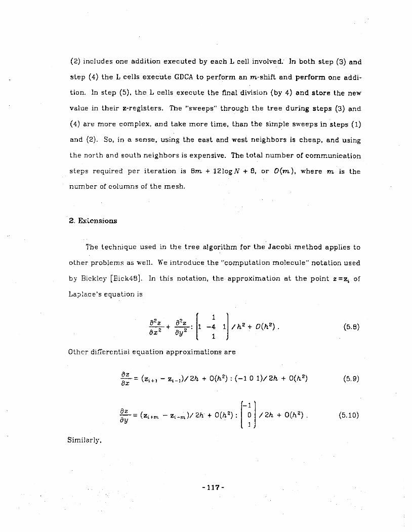
(2) includes one addition executed by each L cell involved. In both step (3) and

step ( 4) the L cells execute GDCA to perform an m-shift and perform one addi­

tion. In step (5), the L cells execute the final division (by 4) and store the new

value in their z-registers. The "sweeps" through the tree during steps (3) and

(4) are more complex. and take more time, than the simple sweeps in steps (1)

and (2). So, in a sense, using the east and west neighbors is cheap, and using

lhe north and south neighbors is expensive. The total number of communication

steps required per iteration is Bm + 12log N + B, or O(m ), where m is the

number of columns of the mesh.

2. E>.."tensions

The technique used in the tree algorithm for the Jacobi method applies to

other problems as well. We introduce the "computation molecule" notation used

by Bickley [Bick4B]. In this notation, the approximation at the point z =z, of

Laplace's equation is

1 -4

1

Other differential equation approximations are

Similarly,

-117-

(5.6)

(5.9)

(5.10)

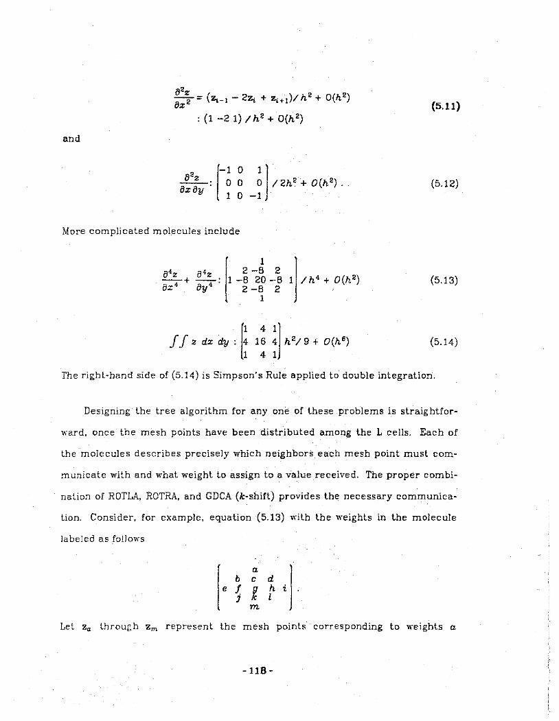
1l2z ' Bx2 = \2:t-t- 2Z; + Z;T!)/ h2 + O(h2)

: (1 -2 1) /h2 + O(h2)

and

More complicated molecules include

I 1

B•z B•z 2 -B 2 --+ --: 1 -B 20 -B ax• ay• 2 -8 2

1

[1 4 11 J J z dx dy : 4 16 4 h 2/9 + O(h 6 )

1 4 1

(5.11)

(5.12)

(5.13)

(5.14)

The right-band side of (5.14) is Simpson's Rule applied to double integration.

Designing the tree algorithm for any one of these problems is straightfor·

ward, once the mesh points have been distributed among the L cells. Each of

the molecules describes precisely which neighbors each mesh point must com·

municate with and what weight to assign to a value received. The proper combi·

nation of ROTL.Ii, ROTRA, and GDCA (k·shift) provides the necessary communica·

lion. Consider, for example, equation (5.13) with the weights in the molecule

labeled as follows

a b c d

e f. h i J 1 l

m

Let z0 through Zm represent the mesh points' corresponding to weights a.

-118-

through m. The communication requirements between the center point z9

and

each of its neighbors are as follows:

G G G G

RRz9 RR G G G

G

where R represents a ROTRA or ROTLA and G represents a GDCA. Each applica-

lion of ROTLA and ROTRA requires 2log N + 2 communication steps and each

application of GDCA (k-shift) (or GDCA (-k-shift)), 1.;bdmn/2l, requires at

J11ost 4 k + 4log N + 2 communication steps. Thus, we need at most

Value Operation Steps Obtained

Zn • Zi 2xROTLA 4!ogN+4 Ze, Zf 2xROTRA 4logN + 4 Zo, Z1 2 x GDCA(m + 1) B(m+1) + BlogN + 4 Zc, Zk 2xGDCA(m) 5(m} + BlogN + 4 Zj, Za 2 x GDCA(m -1) B(m-1) + BlogN + 4 z.,. z, 2xGDCA(2m) B(2m) + BlogN + 4

Total 40m + 40logN + 24

communication steps, where m is the number of elements of one row in the

mesh (the distance between Zc and z9 , for example), n is the number of ele­

ments in one column, and N=2P, p =flog mnl.

This straightforward algorithm can be improved. For example. four GDCA's

are required to send Za, z 0 • Zc, and Za individually to z9 . Instead, we can use

GDCA (m) to send z., ROTRA to send z0 , and ROTLA to send Za to the L cell con-

taining Zc, have this L cell lake the weighted average of all four points (z., z0 ,

Zc, and Za. whose weights are a. b, c, and d, respectively), and use GDCA (m) to

send the result to the L cell containing z9

. Similarly, we can use ROTRA, ROTLA.

and two applicaliom of GDCA (m) to send the weighted average of points z1. zk.

-119-

z1, and Zm lo the L cell containing Zg. We would need a total of only 4 GDCA's and

B RDTRA's or ROTLA's:

G G R R

R R R

z9 R R G R

and total communication time would be

Va.lue Obtained

Operatum

2xROTRA 2xROTLA

G

Za. z, , Zc, Za ROTR<\, ROTLA (combined) 2xGDCA(m)

Z;. Zr., Zt, Zm ROTR<\, ROTLA (combined) 2 x GDCA(m)

Total

Steps

4logN + 4 4logN + 4

4logN + 4 B(m) + BlogN + 4

4log N + 4 B(m) + BlogN + 4

16m + 32logN + 24

or a reduction by approximately 60%. Further improvements are possible (note

that every L cell receives the values of its east and west neighbors three times)

but these improvements would reduce only the log N term of the equation. No

further reduction on the high-order (m) term appears possible.

3. Jacobi Over-relaxation

The Jacobi over-relaxation, or JOR, method is similar to the Jacobi method

except that we use a parameter"' to "correct" the new iterate. For example, for

Laplace's equation, we use

(5.15)

instead of (5.5) to improve each interior point. The method of choosing the

-120-

relaxation parameter :.> is described by Young [Youn71]. Note that :.> is a con-

stant determined before the first iteration. The first four steps of the tree algo-

rithm for JOR are identical to those of the Jacobi tree algorithm. Step (5) of JOR

proceeds as follows.

(5) An L cell containing an interior mesh point replaces the old z value with a

new one using equation (5.15).

We assume each L cell computes the constant quantities :.>/4 and 1-:.> once at

the start of the process and then retains them. The T cell directories used in

GDCA are also determined only once and retained throughout.

The analysis of one iteration of JOR is shown in Figure 5.5. Step 5 of JOR

requires an additional two multiplications and one addition of the term

(1-c.>)zfil. One iteration of this method requires O(m) time.

4. Gauss-Seidel and Successive Over-relaxation

The Gauss-Seidel and successive over-relaxation (SOR) methods are similar

to the Jacobi and JOR methods. respectively. except that the new value zfi+I) is

used as soon as il is available. Thus equations (5.5) and (5.15) are replaced by

(5.16)

and

._(j+I) = c.:(zfi+I) + zU•I) + .,(i) + zUl )/4 + (1-:.>)z.(i) ~ 1.-m ,-1 -,.Tl 1.+m 1. (5.17)

respectively.

Mesh points are modified in row-major order with new values used as soon

as available. One pass through the entire mesh constitutes one iteration.

-121-

Figure 5.6 gives a snapshot of the mesh midway through an iteration (circles

represent points that have already been modified). The new value of Zt is

currently being obtained. The Gauss-Seidel method is known to have twice the

convergence rate of the Jacobi method [Ames77), and, on sequential computer,

it is preferable. lt is unfortunate, however, that the Gauss-Seidel method lacks

the feature that made the Jacobi method attractive for parallel computation,

i.e., the possibility of replacing all interior point values simultaneously. Gauss­

Seidel seems to be inherently sequential.

After a closer examination, however, we discover that it is possible to intro­

duce some parallelism into the Gauss-Seidel method. Referring once again to

Figure 5.6 and the sequential Gauss-Seidel algorithm, we first observe that after

z 10 has been modified, it is possible to modify both z 11 and z 19 . If we consistently

apply the rule that, after modifying Z;. we modify points Z;+l and zi+m• we see

that instead of improving a single point at a time, we can improve an entire diag­

onal of points simultaneously (Figure 5.7). We have the image of a wave front,

moving from the norlhwest corner toward the southeast corner, and improving a

diagonal values at each time step. One iteration is the time required for the

wave to move over the entire mesh.

\re also observe that after a diagonal row of points has been modified, it is

again ready for improvement in the second time step following. In Figure 5. 7,

step 3, for example, as we obtain z~P· zfbl, and zW. i.e., the first approximations

of z28 , z20, and z 12, we may also obtain z f5l. In general, after z,'l) is obtained, it is

possible to im;orove this value at every other time step. Figure 5. 7, step 11,

shows the entire mesh with different points at different stages of improvement.

A circle indicates that a mesh point is currenlly being modified. The point z 10 is

-122-

undergoing its sixth modification while z52, in the lower right hand corner, is

going through its first. From now on, at each step, half of the mesh points are

modified. One iteration, i.e., the time required to modify the entire set of

points, takes h\'0 steps. The tree algorithm proceeds as follows.

(0) Startup. At each step, we obtain the first modification of a diagonal of

points, starling from the northwest corner (z10 ) and proceeding toward the

southeast corner (z52). After a diagonal of points is modified the first time,

it may be modified again at every other step.

After the southeast corner has been modified the first time, every step modifies

approximately half the number of mesh points. This involves the following

operations.

(1) Use ROTL.It to send the value of L(i+l)rnod mn to L;.. Each mesh point receives

the value of its ::::tst neighbor. Each L cell executes t :=value received.

(2) l..'se ROTRA to send the value of L(i-l)mod mn to L;,. Each mesh point receives

the value of its west neighbor. Each L cell executes t := t + value received.

(3) Use GDCA( -m-shift) to send the value of L(i+m)mo:i mn to L;,. Each mesh

point to be modified receives the value of its south neighbor. Each L cell

executes t := t +value received.

(4) Vse GDCA(m-shift) to send the value of L(i-m)mo:i mn to L;. Each mesh point

to be modified receives the value of its north neighbor. Each L cell exe­

cutes t := t +value received.

(5) An L cell containing an interior mesh point computes a new z-value: z = t /4

(equation (5.16) ). L cells containing boundary points and L cells containing

interior points which are not to be modified in tbis half-iteration do nothing

wilh the information they receives.

-123-

After step 5, approximately half of the points have been modified. Steps 6-10

apply the same algorithm on the rest of the points. The analysis of one iteration

of this algorithm, after the startup step, is shown in Figure 5.8. In each half­

iteration, the time required to perform a GDCA is approximately half that usu­

ally required for an m-shift. This is because only half of the points send values

each time, hence only half of the amount of data must pass through the tree

branches. One iteration of this method requires O(m) time.

The same technique can be used with the SOR method as easily as with the

Gauss-Seidel method. We replace step (5) of the Gauss-Seidel algorithm with

(5) An L cell containing an' interior mesh point computes a new z-value:

z =c.; t /4 + (1-w)z.,Cil (equation (5.17)). L cells containing boundary points

and L cells containing interior points that are not to be modified in this

half-iteration do nothing with the information they receive.

Step (10) of Gauss-Seidel is similarly modified to obtain step (10) of SOR. The

analysis of one iteration of point iterative SOR, after startup, is shown in Figure

5. 9. One iteration of this method requires O(m) time. It is interesting to note

that in each half-iteration, the points that are modified and the points that are

not form a checkerboard pattern on the mesh. This pattern, sometimes called a

red-black ordering of the mesh points, is well known and is described in the next

section.

5. Rcd-b!&c~ Ordering of Mesh Points

Young [Youn71] has found that, in some cases, it is possible to change the

order in vchich mesh points are improved "·ithout redudng the convergence rate

of the iterati,·e method used. One may, for example, arrange the points into two

-124-

groups {"red" and "black") such that if a point is red (black), all of its neighbors

are black (red). Figure 5.10 shows how the points are organized, with triangles

and circles representing red and black points respectively. Instead of trying to

modify the values of all of the points simultaneously, we modify each group of

interior points alternately, using either the Gauss-Seidel (5.16) or SOR (5.17)

equations. This, in effect, breaks one iteration of the Gauss-Seidel or SOR

methods into two half-iterations, each of which improves the values of approxi-

matcly half the set of points. The higher convergence rate of red-black Gauss-

Seidel or red-black SOR [Youn71] over the Jacobi method makes red-black ord­

ering attractive. Lambiotte and Voigt [LaVo75] have reported that the applica-

lion of red-black SOR to solve tridiagonal linear systems produces the same con-

vergence rate as regular SOR.

Consider equation (5.17) used in straightforward SOR. When applied to a

red-black ordering of points. equation (5.17) is broken up into two equations

(5.18)

used for all "red" points z., and

zU+I) = (.)(zU+I) + zU+I) + z.U+I) + zU+Il); 4 + (1-(.))z (i) ~ t-m •-1 t+l ttm 1. (5.19)

used fer all "black'' points z,. 1'\ote that the variables Z.-rn, z,_ 1, Zi+I• and Zi+m in

equation (5.18) are black points, whereas the same variables in equation (5.19)

are all red points. In each half-iteration, all of the data required to compute new

values are known and the only problem is communication. The communication

requirements, in fact, are exactly those required by the Jacobi method, except

that only half of the points are sent through the tree each time. Each L cell has

a mask to distinguish red points from black points.

-125-

The analysis of one iteration of this method is identical to that of point

iterative SOR (Figure 5.9). The total time to perform the GDCAs is approxi­

mately the same as required in one iteration of the Jacobi method. Each itera­

tion of red-black SOR, however, requires twice the number of ROTLA's and

ROTRA's.

C. Elock iterative Methods

Section B presented methods that, when implemented on a sequential com­

puter. modify a single point at a time. This is possible because the value at any

point is expressed by an explicit equation involving the point's neighbors. Point

iterative methods can be extended naturally to block iterative methods (also

called l-ine methods, group methods, or implicit methods) which modify a block,

line, or group of points at a time. This usually means that we must solve a sys­

tem of equations for each block. Ames [Ames77] reports that the redefinition of

an explicit method into an implicit method often improves convergence at the

expense of more computation per iterative step.

Jn this section, we take each of the point iterative methods described in

Section B and present its block iterative counterpart. We define a block to be a

row of points. The problem we examine is the solution of Laplace's equation on a

rectangular region using the five-point computation molecule.

1. Line Jacobi

This method represents each of the points in a row by the following equation

-126-

(5.20)

where Z; represents an interior mesh point. The equation involves the (j + l)th

approximation of the points z;. Z;_ 1, and Z;+t and the jth approximation of Z;-m

and Z;+m (the two latter values are assumed to be known). Each equation

involves at most three consecutively indexed unknowns (points adjacent to the

left or right boundaries involve only two unknowns). The equations correspond­

ing to a row of points form a tridiagonal linear system. If each row is

represented this way, we obtain n independent tridiagonal systems. Moreover,

because the mesh points are initially distributed among the L cells in row major

order, a row of points occupies consecutive L cells, except possibly for inter­

spersed empty L cells. Different tridiagonal systems, therefore, occupy non­

overlapping sequences of L cells and the solutions of all of these systems may be

obtained simultaneously using one of the direct tridiagonal system solvers

described in Chapter 3. The algorithm is, in fact, simpler as the tree machine

need not distinguish betv.-een different tridiagonal systems. The n tridiagonal

systems do not overlap and thus may be considered one large system. The

coefficients of the first and last mesh points of a row prevent one system from

interfering with another. The ability to make this simplifying assumption on a

tree machine is discussed in Section 4.D.

As with the point iterative Jacobi method, we assume the fol!ow·ing. Boun­

dary points are distinguished from interior points by a mask in the L cell. If an

interior point is contained in l;, then its north and south neighbors lie in L;-m

and L;+m and its west and east neighbors lie in !.,__ 1 and L;+t· Moreover, each L

cell contains the registers a, b, and c in which we store the coefficients of one

tridiagonal equa~ion. Let L1, contain Zi· The follo~.\·ing algorithm determines the

values of a, b, anC: c for different mesh points.

-127-

if z; is a boundary point then a=b =c =0

else if z,_ 1 is a boundary point then a=O. b=-4, c=l

else if z,. 1 is a boundary point then a=l. b=-4, c=O

else a=l, b=-4. c=l

The tree algorithm proceeds as follows:

z;'s west neighbor is a boundary point

z, 's east neighbor is a boundary point

neither of Z; 's east or west neighbors is a boundary point

(1) l:se GDCA(m-shift) to send the value of L(i-m)mo<tmn to L;..

(2) Use GDCA( -m-shifl) to send the value of L(i+m)moa mn to L;_.

The 1'Um of the values obtained in steps (1) and (2) determine the constant term

of each linear equation. Each L cell now has all of the information it needs to

construct the linear cqualion (5.20) representing one interior mesh point. We

are ready to solve then tridiagonal linear systems.

(3) Let all L cells participate in a single application of one of the direct

methods for sol\ing a tridiagonal linear system (Chapler 4). Then tridiago-

nal systems are considered one.

An iteration ends with step (3). The analysis of the line Jacobi method is shown

in Figure 5.11. One iteration of this method requires O(m) time.

2. Line J;::.cobi Over-relaxation

Line JOR is similar to line Jacobi except that we introduce a relaxation

parameter r.J and use

-128-

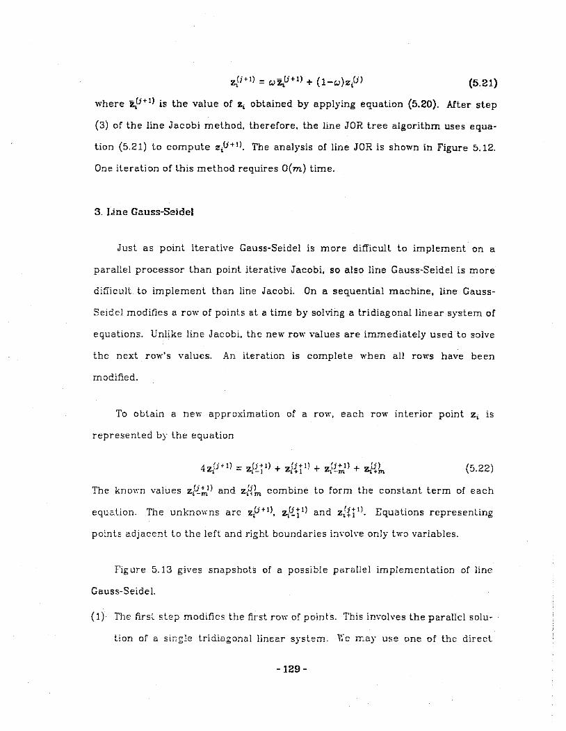
z,0• 1l = r.>Z;.(j+t) + (1-r.>)z/il (5.21)

where z,U+t) is the value of Z; obtained by applying equation {5.20). After step

{3) of the line Jacobi method, therefore, the line JOR tree algorithm uses equa­

tion {5.21) to compute zp+t)_ The analysis of line JOR is shown in Figure 5.12.

One iteration of this method requires O{m) time.

3. Line Gauss-Seidel

Just as point iterative Gauss-Seidel is more difficult to implement on a

parallel processor than point iterative Jacobi, so also line Gauss-Seidel is more

difficult to implement than line Jacobi. On a sequential machine, line Gauss-

Seidel modifies a row of points at a time by solving a tridiagonal linear system of

equations. Unlike line Jacobi, the new row values are immediately used to solve

the next row's values. An iteration is complete when all rows have been

modified.

To obtain a new approximation of a row, each row interior point z; is

represented by the equation

4zU+tl = zU+t) + zU+tl + z(i+t) + .._(j) ~ t-1 t+l t-m -.+m (5.22)

The known values zU+t) and z{il combine to form the constant term of each t-m t1m

equation. The unkno\rns are zP+l), zl~tt) and z[~tn. Equations represenLing

points adjacent to the lefl and right boundaries inYol,·e only bm variables.

Figure 5.13 gives snapshots of a possible parallel implementation of line

Gauss-SeideL

{1) The firsl step modifies the first row of points. This involves the parallel solu-

tion of a single tridiagonal linear system. We rnay use one of the direct

-129-

methods for solving tridiagonal systems described in Chapter 4.

(2) The second step modifies the second row of points. Again, this involves the

solution of a single tridiagonal linear system.

(3) The ith step, i =3, 4, ... , n where n is the number of rows of interior mesh

points, modifies the ilh row of points. In addition, we may also modify the

jth row of points where j=i-2, i-4, ... , 2 or 1. This means that after the

ith row of points is modified the first time, it may be modified again at

every other time step. As i increases, therefore, so does the amount of

parallel activity.

After the last row of the mesh is modified the first time, then at every step,

a.pproximately half of the rows are modified, i.e., we alternately modify odd­

indexed and even-indexed rows. Kote that the parallel implementation of point

iterative Gauss-Seidel or red-black SOR produced a checkerboard pattern on the

mesh whereas with line Gauss-Seidel, a striped pattern is produced. The ith

iteration (i > n =the number of mesh rows) of the tree implementation of line

Gauss-Seidel proceeds as follows.

,:fod.ify od.d.-inde:::ed rou;s,

(1) L'se GDCA(m-shift) to send the value of L(i-m)mo<Jmn to L;. Only points on

even-indexed rov1s send a value.

(2) L'se GDCA(-m-shift) to send the value of L[i+m)moamn to L;. Only points on

even-indexed ro ... n:; send a value.

The sum of the velues obtained in steps (1) and (2) determine the constant term

of each linear equation.

(3) All L cells whose mesh points line on odd-ind~xed rows participate in the

solulion of a single thdiagonal system. As with line Jacobi, the coefficients

-130-

of the end interior points of a row prevent the different tridiagonal systems

from interfering with each other.

Modify even-indexed rows.

(4) Use GDCA(m-shift) to send the value of L(i-m)moamn to L;. Only points on

odd-indexed rows send a value.

(5) Use GDCA(-m-shift) to send the value of L(i+m)modmn to L;. Only points on

odd-indexed rows send a value.

The sum of the values obtained in steps (4) and (5) determine the constant term

of each linear equation.

(6) All 1 cells whose mesh points line on even-indexed rows participate in the

solution of a single tridiagonal system.

The analysis of line Gauss-Seid8l is shown in Figure 5.14. One iteration of this

method requires O(m) time.

4. Line Successive Over-Telaxation

The technique used in line Gauss-Seidel may be used to solve the block­

tridiagonal system using line SOR. Instead of equation (5.22), we use

(5.23)

where z[i+I) is the value of Z; obtained b applying equation (5.22) and r.> is the

relaxation factor. The algorithm for line SOR is similar to that for line Gauss­

Seidel except that equation (5.23) is evaluated after steps 3 and 6. The analysis

line SOR is shown in Figure 5.15. Steps 3a and 6a (during \\'hich equation (5.23)

is evaluated) each require two multiplications O'lnd one addition. One iteration of

this method requires O(m) time.

- 131-

D. Alternating Direction Implicit Method

A method by Peaceman and Rachford [PeRa55] and a related method by

Douglas and Rachford [DoRa56] improve on block iterative methods by modify-

ing rows of points in one half-iteration and columns of points in the next half-

iteration. .Ames [Ames77] reports that this often produces better convergence

than straightforward block iterative methods which modify points a row at a

time. Ee states, however, that a "rational explanation ... of the efTecliveness of

ADJ methods is still Jacking." A survey report on ADl methods was presented by

!lirkhoff, Varga and Young [BiVY62]. The following description is based on the

study by Ames [Ames77].

Basically, ADl methods perform a single row iteration on the mesh followed

by a single column iteration. To perform a row iteration, we represent each row

interior mesh point by

z u + 1;2) = z rJl+p. [z u + 1/2) + z u + 11 2'-2z (J + 112l]+p .[z(il + z Ul -2"'.u ,)] (5. 24) 1. ' J •-1 1.+1 ~ ;_ t-m ;.tm ~

where Pi is called the iteration parameter which may vary with j. This defines a

tridiagonal linear system whose solution produces a row of new values. After

each row has been modified in this manner, a column iteration is performed.

The interior points of a column are each represented by the equation

Z Ci + l)_ z.{i + 11 2) +p. [z U + 11 2)+ zU + t/2)._2z U + 11 2)]+p. [zU + 1)+ z (i + I)_zzU +1)](5 25) o. - " ; L-1 ttl 1. J 1-m 1.+m 1 ·

This also defines a tridiagonal system whose solution produces a column of new

values. A mod1ficalion of each row foJlo;,·ed by a modification of each column

constitutes one complete iteration.

As before, the mesh points are distributed am"ng the L cells in row major

order. Consider a mesh wilh n ro"'s, numbered 0 through n-1, and m columns,

-132-

numbered 0 through m -1. The points belonging row i occupy L cells with

indices im, im+1, im+2, ... , im+(m-1). On the other hand, points belonging to

column i occupy L cells with indices i,i+m,i+2m, ... ,i+(n-1)m. Because of the

decision to distribute the points in row major order, rows of points are contained

in non-overlapping sequences of L cells. Columns of points, however, are con-

tained in overlapping L cell sequences. This allows the tree machine to perform

row iterations much faster than column iterations.

To implement a row itera.tian, we first observe that the tridiagonal linear

systems produced by equation (5.24) are uncoupled, i.e., the solution of the

j + 1/2 approximation of row. i depends only on the j th approximation of the

rows i-1 and i+l. (Contrast this to line Gauss-Seidel and line SOR in which the

(j + 1)th approximation of row i depends on the (j + 1)th approximation of row

i-1 as well as the jth approximation of row i+l.) This means that we can solve

all row tridiagonal systems simultaneously. Moreover, because the tridiagonal

systems are uncoupled, we may consider all of the tridiagonal systems as forme

ing a single tridiagonal system (discussed in delail in Section 4.D). A single

application of one of the tridiagonal system solvers described in Chapter 4 on

the entire tree solves all of the tridiagonal systems involved simultaneously. The

tree algorithm for a single row iteration proceeds as follows.

(1) l!se GDCA(-m) to send the value of L[i+m)mo~ mn to L;. L; receives the value

I') Zdm·

(2) l:se GDCA(m) to send the value of L[i-m)ma~ mn to Li. L; receives the \'alue

zUl . t-m·

(3) Each L cell computes the constant factor of equation (5.25):

-133-

·and sets up the coefficients of the linear equation corresponding to point· z,.

(4) Apply one of the direct tridiagonal linear system solvers described in

Chapter 4. At the end of step 4, the L; contains zfi+l/ 2) defined by equation

(5.24).

Column iterations are slower than row iterations. The reason is that

columns of points, and hence the corresponding tridiagonal systems, lie in over-

lapping sequences of L cells. Although we can obtain new iterates for a single

column of points as easily as we can for a single row of points {by masking all

other columns out), we cannot solve tridiagonal systems corresponding to two or

more columns simultaneously, because their computations would interfere v.ith

each other. \\'e can, however, separate these computations in time, and solve

the tridiagonal systems of the columns one after another. The tridiagonal sys-

tern of one column may be solved in parallel in O{log n) time. As there are m -2

columns of interior points, a column iteration requires O{m logn) time. The

tree algorithm for a complete column iteration proceeds as follows.

(5) Use ROTLA to send the value of L(;+ 1)moo mn to L;. L; receives the value

Z (j+l/2) >+1

{6) Use ROTRA to send the value of L(;-1)m•• mn to 4· L; receives the value

Z (i+ 1/2) i-1

(7) Each L cell computes the constant factor of equation (5.25):

Z U + 11 2l+p. [z U + l/2) +z.U + l/2l-2zfi + 11 2)] 1. ) ,-] 1.+1 1.

At this point, the 1 cells are ready to solve the (column) tridiagonal systems

defined by equation (5.2:0). \'ie must, ho1\·ever, solve one tridiagonal system at a

time. J.e., step 8 is a loop over the columns of the mesh.

-134-

(B) For each column, use one of the direct methods described in in Chapter 4

to solve a column tridiagonal linear system. At the end of step B, L;, holds

zli*') defined by equation (5.25).

The analysis of the tree implementation of the ADl method is shown in Fig­

ure 5.16. Row iterations and column iterations are carried out in steps 1-4 and

steps 5-6, respectively. A row iteration requires O(m) time because the solution

of all of the tridiagonal systems (step 4) can be done simultaneously. A column

iteration, however, requires O{mlogn) time because each of the m tridiagonal

systems must be solved in turn. One complete iteration of the ADl method,

therefore, requires O(m log n) time.

E. Remarks

Figure 5.17 shows the convergence rates of several point iterative and block

iterative methods, as described by Ames [Ames77]. Table entries give the value

R; the number of iterations required for convergence is inversely proportional to

R.

Figure 5.18 gives a summary of the analyses of the point iterative, block

iterative, and AD! methods discussed. On a sequential computer, a block itera­

tive method converges faster than the corresponding point iterative method

(e.g. block Jacobi converges faster than point Jacobi) but involves more compu­

tation. On a tree machine, block iterative methods also involve more computa­

tion, but lhe lola! computation time is still significantly less than the communi­

cation time. For a large mesh (m and n large), the significance of the increased

computation time diminishes, i.e., block iterative methods may not require

significanlly more time than point iterative methods. In summary, we can say

-135-

that on a tree machine, a block iterative method looks m·ore attractive com­

pared to the corresponding point iterative method than on a sequential com­

puter.

F. Detailed Time Analyzis of the Jacobi Method

This section presents a detailed analysis of the Jacobi method for solving

Laplace's equation (5.6) implemented on a tree machine, and compares the per­

formance of the tree machine with that of a sequential computer. We assume

that the tree machine has the following characteristics.

(1) The (DEST#. V.II.Ll.!E) pairs sent through the tree during an application of the

GDCA algorithm are 84 bits long, a 20-bit DEST# and 64-bit floating-point

VALliE.

(2) Communication is two-way, and the channels connecting a cell to its father

or sons are k bits wide, where 64/k is an integer.

(3) The tree has 220 L cells, thus allowing the use of a mesh with 220 mesh

points. For the sake of simplicity, we assume a square mesh with 210 rows

and 2 10 columns.

On a sequential computer, each iteration of the Jacobi method requires the

follovcing operations to be performed for each interior mesh point.

(l)c(3) Add the values of the a point's four other neighbors.

(4) Divide the sum by 4, produced by a shift operation.

For the sake of simplicity, we assume that each floating-point operation requires

the same amount of time. The number of interior mesh points is

-136-

(21°- 2)(2 10 - 2). One iteration of the Jacobi method, therefore, requires

(5.26)

floating-point operations per iteration.

The tree machine requires five operations: (1) ROTLA, (2) ROTRA, (3)-(4) two

applications of GDCA, and {5) one shift operation to perform the division by 4.

VIe assume that the T cell directories required by GDCA are already in place. If

the time required for one cell to send one bit to an adjacent cell is T, then the

time required by ROTLA, ROTRA, and GDCA (Chapter 3) are

ROTL.~: [(2logN + 2) + (64-k )I k] T

ROTRA: [(2logN + 2) + (64-k)/k]T 2x GDCA: [2(4logN + (2(20 + 64)m -k)!k)]r (5.27)

Total : [(BlogN + 4) + (2!k)(16Bm -2k + 64))T

where log .II'= 20, m = 2 10. ROTLA and ROTRA require the time for one 64-bit

floating-point number to go through the C cell and hack down to an L cell.

Because the channels are k bits wide, the entire number reaches the destination

L cell {64-k )/ k time units after the first k bits arrive. Each application of GDCA

requires {at most) the time form (DEST#. VALt:E) pairs to go through the root T

cell and back down to the destination L cells. A (DEST#. VALUE) pair is 84 bits

long. Since a sequential computer requires approximately 4 million operations,

the performance of the tree machine in millions of floating-point operations per

second (MFLOPS) is approximately

(number of arithmetic operations) I (time on a tree machine) =

(4x 106 ) [( )] :::: 1.16x 10-5 (k/T) !.:FLOPS.

BlogN + 4) + (2/lc){16Sm -2k + 61 T

Figure 5.19 shows lhe performance of a tree machine executing one iteration of

-137-

the Jacobi algorithm fork = 1. 2, 4 and 'T= 40, 60, eo. 100 na:rioseconds.

The performance of a tree machine is even better if we use red-black SOR - '

(5.18-19) to solve the problem. Since communication requirements on a tree

machine remain approximacleJy lqe_ si:Ulle but the number of operatipns on a

sequential computer increases from apprpxirnat~y 4 m,illion to approxiplately 6

million performance increases by appro~imately 50%.

-130-

•

...

•

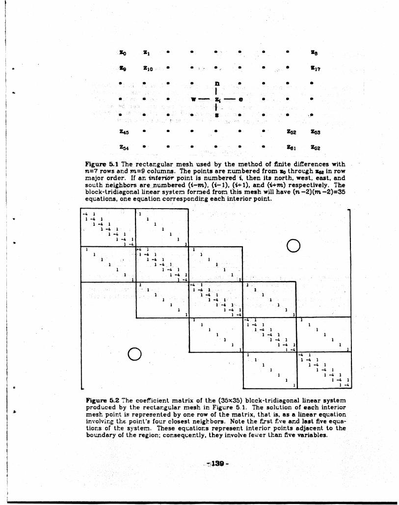
:.Jo zs • • • -.. ·• • • Sa

,_itlg Zto -..; . • • l • • • • •n " .. ·.;~

•- J• • • D • • • • "<

J "

• • '· • ·-- Zi - • • • • ';._;,;'} l -·

• • • '• ., ·;· • .. .~ ·;· t .'tl;"·

Zt-5 • • • • • • Z52 Zos

~4 • • • • • • Set Zo2 .;<,.

FigUJ"e 5.1 The_ rec;ta~gl.).lar_m_~sh used by the tnethod of finite difierences with n=7 rows and rn=-9 coJum~. The points are nunsbered from-so through zu in row major order~ If lin inte~ point is numbe-red'i. then its north, west; east, and south neigh:~rs are __ J1Q.J'Xlbered (i-m), {i-:-1). {i-+1), and (i+m) respectively. The block-tridiagonal linear sy~tter:i formed froJ:l ibis mesh will have (ti -2)(m -2)•35 equationS, one eq-cation correspondir.,g each iri~erior point.

;, -4 1 -1

'

1 -4 l 1 1 -4 1 1

1 _,.

1 ; 1 1 •4 1 1

1 -4 1 1

0 1 -4 l I ; ,.4 l 1

1 ---1 -·

} 1 1 :_I ii 1 -4 1 1

1 l -4 I ~ ----1 1 -4 1 i

1 i l -4 t 1 ,, 1 ._, :r'· ' -l """ . 1 1 -

-< '1 1.-fo l. ·-. .. _I

; 1 1_-4 1 i

1 ' 1 _, 1- 1 1 l ·-4 :1.'' ·' 1'

1 1 _, 1 1 1 1

_, 1

• •4 1 1 1 'l -4 1 1

1 1 -4 1 1 1 1

_, 1 1

1 1 -4 1 1 J 1 -4 1 l

0 1 I -4 _l

1 -4 1 t- 1 -4 1

1 1 -4 1 1 1 -4 1

1 l' -4- 1 J 1 -4 1

J J -4

Figure 5.2 The coef!icient matrix of the (35X35) block-tridiagonal linear system produced by the reclar..gular mesh in Figure 5.1. The solution of each interior mesh point is represented by one row of the matrix, that is, as a linear equation in\'olving the point's four closest neighbors. Notethe fJst Eve ar.d last five equa-:­tions of the system. These eq~atior.s represent interior points adjacent to the boundary of the region; conseq-cenlly, they involve fev;er than five Ve.ritables.

1 cells: 0 0 0 0 0 0 0 0

seq#: 0 1 i-m i-1 i i+l i+m mn.

Figure 5.3 Initial layout of the mesh points among the L cells. In the Jacobi method, the ith L cell must communicate with its north, west, east, and south neighbors, which are in the (i-m)th, (i-l)th, (i+l)th, and (i+m)th L cells, respectively. Communication with its east and west neighbors can be accom­plisl'ed with ROTLA and ROTRA. Communication with its north and south neigh­bors requires GDCA performing an m-shift to the left.and also to the right.

Point Jacobi Parallel Operations

Step Swps Comm. Time 1 cells T cells C cell

+ X + X + X

1. ROTLA 1 2logN+2 I ~ I 0 0 0 0 0

1

2. ROTRA 1 21ogN + 2 0 0 0 0 0 , 3. GDCA 1 4m + 4logN + 2 1 0 0 0 0 0 ' 1 (-m-shift) : 4. GDCA 1 4m + 4logN+ 2 1 0 0 0 0 0 I (m-shift)

15. 0 L

0 0 1 0 0 0 0

I Total I 4 Bm+ 12logN + 8 I 3 1 I 0 0 0 01

Figure 5.4 Ar_alysis of one iteration of the Jacobi method solvirog Laplace's equa­tioro oro a rectarogdar mesh with n. rows and m colur::ms. N=Z', p = llogmnl, that is, N is the r.tcmber of L cells of the smallest tree machine that can hold mn. poir:ts. This analysis does net include the time required to cor:struct the T cell directories. 'lhe total cor:u:'lt:r:icalion time is O(m ).

: -140-

Point Jacobi Over-relaxation Parallel Operations

Step Swps Comm. Time L cells T cells C cell

+ X + X + X

1. ROTLA 1 21ogN+ 2 0 0 0 0 0 0 2.ROTRA 1 21ogN + 2 1 0 0 0 0 0 3. GDCA 1 4m + 4logN+ 2 1 0 0 0 0 0 { -m-shift)

14. GDCA 1 4m+4logN+2 1 0 0 0 0

I 0

1 (m-shift) 5. i 0 i 0 1 2 0 0 0 0

Total I 4 Jsm+12logN+8 I 4 2 I 0 0 0 0

Figure 5.5 Analysis of one iteration of the JOR method solving Laplace's equation on a rectangular mesh with n ro'"s and m columns. This figure differs from Fig­ure 5.~ or:ly in step 5. JOR requires one more addition and multiplication per iteration than the Jacobi method.

zo zl z2 zs z4 z5 ze z7 Za

Zg 0 0 0 0 0 0 0 Zn

Z18 0 0 0 0 0 0 0 Z2s

Z27 0 0 0 Zi • • • Z3o

Z3s • • • • • • • z«

Z45 • • • • • • • Zos

Z;;4 Zoo Z5s Zo7 z=:a Zos Zso Zs1 Zs2

Figure 5.6 Sr:apshot midway through or:e iteration of the sequential Gauss-Seidel algcrilbn. lr:tericr J:J.csh poir.ts are ncdified ·in row-major order wit:t: the new Yah.:.e of a point ir.1mediately t:.sed to obtain the new vah.:e of the r:ext point. A circle ir:dicates lLat a poir:l has been r:wdif.ed; tl:e next point to be modified is Zzt· Modifying all of the interior points constitutes one iteration.

-141-

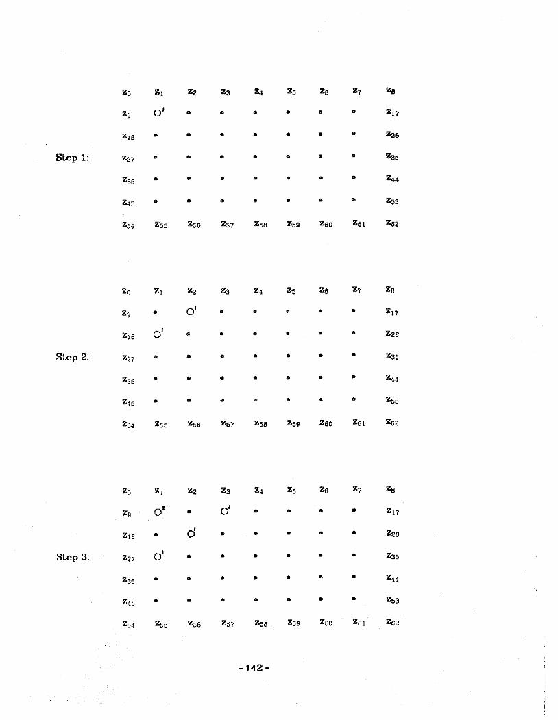
zo z, Z2 zs Z4, Zs ze Z7 za

Zg o' 0 • • • • • z,7

z,e • • • • • • • Z2e

Step 1: Z27 • 0 • • • • • Zso

Zss • 0 • 0 • • • z44

Z.s • • • • • • • Zss

Zs4 Zss Zoe Zs7 Zse Zss Zeo Zs1 Zs2

zo z, Z2 zs z. Zs zs Z7 Ze

Zg • o' • • 0 • • ZJ7

z,e o' • • • • • • Z2s

Step 2: Z::7 • • • • • • • Zss

Z35 • 0 • • • • • z44

Z45 • • • • • • • Zos

z,. Z~5 Zss Zs1 Z55 zss Zeo zs, Ze2

zc z, Z2 zs z. z, Zs Z7 ze

Zg o• • o' • • • • zl1

z,a • d • • • • • Z2s

Step 3: Z27 o' • • • • • • Zss

Zss • • • • • • • z ••

Z.s • • • • • • • Zss

Z::4 z~5 Z:;s Z::;? Z5a zss zsc zs, Za2

-142-

Zo z, Zz zs Z4 Zo za Z7 za

Zg • d • d • • • Z17

z,a o' • d • • • • Zza

Step 4: Zz? • d • • • • • Zao

Zaa o' • • • • • • z44

Z4o • • • • • • • Zos

Zo4 Zoo Zoe Zo? Zoe Zo9 Zeo Ze1 Zaz

•••

Zo z, Zz Zs z. Zo Za z, ze

Zg d' • d • o" • d Zl?

z,a • 0~ • 04- • d • Zze

Step 11: Zz? 0~ • 0 ... • d • 0'2. Zso

Zse • o" • d • o" • Z44 4- d cJ o' Z4o 0 • • • Zoa

Zo4 Zos Zoe z,, Zss Zog Zso Zs1 Zaz

Figure 5.7 Snapsbts during the startt:p period of the parallel Ga>:ss-Seidel algc­rithr:J. Diagonals of paints are modified each lir:1e. In step 1, z 10 is modified the f.rst lime. In step 2, both Z1g and Zu are modified the f.rst tioe. In step 3, Zzs, z2c ar:d z 12 are r.wdified the first tioe and z 1o is modified the second time. In ger:eral, a-fter a poit.l ta.~ beer: nodit1ed c:r..ce, it may again be modified after ever otl:er step. Step 11 shows approximately half of the poil:ls ir: di!Oerent stages of oodification: z 52 the frst tir:Ie, z 50 , z 44 and z34 U:e seccr.d tir:1e, ... , z 10 the sixth tioe. Approxir:Jately half of the points are mod"ified in each step following step 11 ar:d parallelisr:J is at its peak.

-143-

Point Iterative Gauss-Seidel Parallel Operations

Step Swps Comm.

L cells I T cells Time C cell + X I + X + X

1. ROTLA 1 2logN+ 2 0 0 0 0 0 0 2.ROTRA 1 2logN+ 2 1 0 0 0 0 0 3.GDCA I 1 2m+ 4logN + 2 l 0 0 0 0 0 ( -m-shift) I I 4.GDCA I 1 2m+ 4logN+ 2 1 0 I 0 0 0 0 (m-shift) I I

,5. I 0 0 0 1 0 0 0 0

I I

I 6. ROTLA 1 2logN+ 2 0 0 0 0 0 •0 7. ROTRA I 1 2logN + 2 1 0 0 0 0 0 8. GDCA I 1 2m+ 4logN + 2 1 0 0 0 0 0 ( -m-shift) ' ' 9. GDCA

I 1 2m+ 4logN + 2 1 0 0 0 0 0

(m-shifl) I

I I I 110. 0 0 0 1 0 0 0 0 ' I I i ; Total I 8 Bm + 24logJV.+ 16 6 I 2 0 0 I 0 0

Fi&u::-c 5.8 Ar:alysis cf oroe iteration of point iterative Gatoss-Seidel. After the startLCp period (begir:ning with step 11 of Figt:re 5.7, far example), eacl: iteration is achieYed ir~ two steps, sl:cwr.. above as st:.bsfeps 1-5 followed by st:bsteps 6~10. In sc:bsteps 1-5, half of the points receive the valt.:es of tl:eir neigl:bors and are rnadif'.ed. Substeps 3 ar:d ~ sl:cw that the ccnrnunicaticr:tine required for GDCA is apprcxinately half that ust:ally required for ar:. m -stJft. This is because only half of the L cells ser:d vakes arod tl:e arncurot of idcrnatioro coursing through the tree brar:ches is half its usual load.

-144-

Point Iterative Successive OvcrcreJaxalion or Red-Black Successive 0-;;er-relaxation

Parallel Operations

Step Swps Comm. Time L cells T cells C cell

+ X + X + X

1. ROTLA 1 2logN+ 2 0 0

I 0 0 0 oj

2.ROTRA 1 2logN+ 2 1 0 0 0 0 0 3. GDCA I 1 2m+ 41ogN+ 2 1 0 I 0 0 0 0

I { -m-shift) I

4.GDCA 1 2m+ 41ogN+ 2 1 0 0 0 0 0 (m-shifl) 5. 0 0 1 2 0 0 0 0

6.ROTLA 1 2logN+ 2 0 0 0 0 0 0

I 7.ROTRA 1 2logN+ 2 1 0 0 0 0 0 8. GDCA 1 2m+ 41ogN+ 2 1 0 0 0 0 0

i ( -m-shift) i I 1 2m+ 4logN+ 2 1 0 0 0 0 ;9.GDCA

I I 0

i (m-shift) I ol I 0 0 I 1 2 0 0 0 . 10. I I I I Total '

8 J 8m + 24log N + 16 I 8 I 4 [ 0 I 0 I 0 / 0 I li'i~ure 5.9 Analysis of one iteraticr: of poir:t iterative successive over~relaxaticn afler U:e startt:.p period. or one iteration cf red-black s~ccessiYe over-relaxation: Or:e iteration cor:sists of two sub~iteratior..s: one wl-Jch modifies the "triar:gles" (steps 1-5) the other which modif.es the "circles" (steps 6-10). Red-black SOR re­ql:ires twice as mar-y applications of GDCA per iteration as the Jacobi method but each applicatior: takes approximately half the time. Red-black SOR, however, re­qdres hi-lee as mar:y RO-:-LA's and ROTRA's as the Jacobi method. A mask regis­ter ir: eacl: L cell distir:guisl:es triar:gles from circles. Although the complexity of the algorithm is identical, there is a diEerence between the two algorithms. Poid iterative SOR reqwres a startup period whereas red-black SOR does not. Ccr:sequer:tly, dt:rirg or:e iteration of the forP-ter, r:1esh Points have dif'erent ileraticr: r..t:.m.bers (see Figure 5.7) wte:reas d-crir::g one iteralicn of the latter, points nodifled all have the same iteration nmber.

-145-

0 v 0 v 0 v 0 v 0

v 0 v 0 v 0 v 0 v

0 v 0 v 0 v 0 v 0 I

v 0 v o- v- 0 v 0 v I

0 v 0 v 0 v 0 v 0

v 0 v 0 v 0 v 0 v

0 v 0 v 0 v 0 v 0

Figure 5.10 To imple:r:1ent red-black successive over-relaxation, mesh poir:ts are arranged iro a checkerboard (red-black, lriar.gleccircle) pattern. Points of the sane type (all triar.gles or all circles) are modifed sir:n;Jtar.ecusly. One itera-tion, therefore, cor.sists of two sub-iteraticn?:--one which·modifles the ''triar:gles", U:e otter wl:icl: I!lodifies the "circlesn.

-146-

Line Jacobi Parallel Operations

Comm. Step Swps Time L cells T cells C cell

+ X + X +

1. GDCA 1 4m + 4logN + 2 0 0 0 0 0 ( -m-shift)

2. GDCA 1 4m + 4logN + 2 1 0 0 0 0 (m-shift)

3. TA 3 14log N + 14 0 5 10log N 17log N 0

1 Total i 5 I Bm + 22log N + 18 I l I 5. 10log N I 17log N 0 I Figure 5.11 Analysis of one iteratior.. of the line Jacobi method. In steps 1 and 2, the values of a points north and south r..eighbors are received by each interior mesh point. Step 2 includes one addition required to determine the constant term of each point's linear equation. ·In step 3, a single application of the Thomas Algorithm (TA) solves the tridiagor.allinear systems simultaneously. The soh.:tion of the linear systel'!ls provides the new values of ~he mesh points.

Line Jacobi Over-relaxation

X

0

0

1

lt

Comm. Parallel Operations !

Step Swps Time L cells T cells C cell

+ X + X + X

1. GDCA I ( -m-shift)

1

2. GDCA I'

(m-shift)

3. TA

'4. ! I Total

1

1

3 0

5

4m+4logN+2

4m + 4logN+ 2

14logN + 14

0

0

0

5 2

Bm + 22log ]\7 + 1 B [ 3 I B

0

0

lOlog 1~ 1

10 log N

0

0

17log N 0

17log N

0

0

0

0

0

Figure 5.12 Analysis of cr:e iteration of the line Jacobi over-relaxation method. This r:1ethod is similar lo tl:e !iiOe Jacobi r.Jethod (Figve 5.11) but requires ar:: ex­tra step, step 4-, whicl: ccr:1putes each point's ne\Y vah..:..e t:.Sing equation (5.13).

-147-

0

0

1 0

1 I

zo z, Zz zs z. Zs za z? ze

Zg d o' o' o' o' d o' ZJ?

z,s • • • • • • • Zza

Step 1: Zz? • • • • • • • Zso

Zss • 0 D • • • • z ••

Z4[; • • • • • • • Zoa

Zoq Zss Z55 Zo? Zse z'59 Zao zs, Zsz

Zc z, Zz zs z. Zs Zs Z7 Ze

Zg • • • • • • • ZJ7

z,e o' o' o' o' d d d Zzs

Step 2: Z27 • 0 • • • • • Zso

zss • • 0 • • • • z ..

z,5 • • • • • • • Zos

Z;,A Z55 Zss ze? Zoe Zog Zsc ZsJ Zsz

Zo z, Zz Zs z. Zo Zs Z? ze

Zg o• o• r:f cf 02 02 02. z,?

z,e • • • • • • • Zzs

o' o' o' o' o' o' I Slep 3: Zz? 0 Zso

Zss • • • • • • • z ••

Z45 • • • • • • • Zos

ZM Zoo Zso Zo? Zoe Zeg Zso ze, Zaz

-148-

zo zl Z2 Zs z4 Zo Za Z? Za

Zg • • • • • • • zn

04 z 02 02. 6 02. 02. Z1a 0 ~B

Step4: Z27 • • • • • • • Zss

o' d I o' o' o' o' Zaa 0 Z.4

Z45 • • • • • • • Zos

z,. Zoo Zoe Zo? Zoa Zos zso Zs1 Zs2

zo Zz z, za

Zg d • • • • • • •

Step 5: 0~ o'- o•

• • • • • • •

o' 01 01 o' O' Ql o'

Zoa Zo? Zso

Figure 5.13 Block iterative wave snapshots. Sr.apshots dc.rir.g the startt:p period of the line Gac.ss-Seidel algorilr.m. Rows of interior points are modif.ed each time. The Erst and secor:d rows are modif'ed the first time ir. steps I and 2, respectively. In step 3, the third row is modif.ed the first time and the first row is modif.ed tl:e secor:d time. In general, after a .row has been modif.ed orice, it may agair: be r:ocdit:ed after ever other step. Step 5 sl:ows approximately half of tt.e rows ir: diCerer:l stages of modi:f.caUcr:: the :f..fth row is modifled the flrst time, the third row tl:e seccr.d llme, at:d the first row the trJrd Ume.

-149-

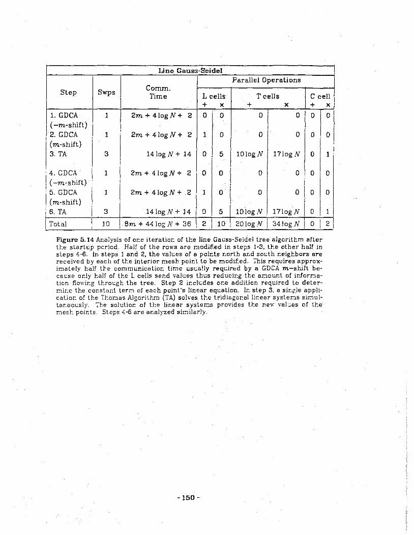
Line Gauss-Seidel Parallel Operations

Cornm. Step Swps

Time L cells T cells C cell + X + X +

1. GDCA 1 2m+ 4logN+ 2 0 0 I 01

0 0 ( -m-shift) I 2. GDCA 1 2m+ 4logN+ 2 1 0 0 ' 0 0 (m-shift) 3. TA 3 14log N + 14 0 5 lO!og N 17log N 0

I 4. GDCA 1 2m+ 41ogN+ 2 0 0 0 0 I

0 I ( -m-shift) '

5. GDCA 1 2m+ 41ogN+ 2 1 0 0 0 0 (m-shifl)

I 6. TA 3 14logN+ 14 0 5 lO!og N 171og N 0

I Total I 10 I Bm + 44 Jog N + 36 2 10 20JogN I 34log N ! 0 i I ' Figure 5.14 Analysis of croc iteration of the line Ga,;ss·Seidel tree algorithm after U·.e slartt:p period. Half of the rows are rnodif.ed in steps 1·3, tr.e other half in steps 4-6. In steps 1 and 2, the values of a points north an.d sot:th r:eigl:bors are received by each of the interior mesl:. point to be r:1odif..ed. ~his requires approx­imately half l~e communicalior: time ust<ally reqt:ir~d by a GDCA m-shHt be· cat:se or.ly half of the L cells ser.d values thus reducir.g the amcunl of informa­tion f.o,rir:g tl:rough the tree. Step 2 ir.cludes one addition required to deter­mir:e the constant term cf each point's linear eqt:;,ation. In step 3. a single appli­cat.ior. of the Tt-_coas AlgcritJ'.cLl (TA) solves the tridiCJ.gor:al lir:ear systeos sir:n~J­tar:eot;.s]y. ';'he solutior.. of the linear sYstems provides the new valties of the mesl: points. Steps ~-6 are analyzed similarly.

-150-

X

0

0

1

0

0

1

2

Line Successive Over-Relaxation Parallel Operations

Comm. Slep Swps

Time L cells T cells C cell + X + X +

1. GDCA 1 2m+ 4logN + 2 I 0 0 0 0 0 ( -m-shifl) 2. GDCA 1 2m+ 4logN+ 2 1 0 0 0 0 (m-shifl) 3. TA 3 14log N + 14 0 5 10log N 17log N 0 3a. 0 0 1 2 0 0 0

' i 4. GDCA 1 2m+ 4logN+ 2 0 0 0 0 0 I ( -m-shifl) 5. GDCA 1 2m+ 4logN + 2 1 0 0 0 0

1 (m-shifl)

I 16. TA 3 14logN+ 14 0 5 10logN 17log N 0 1 6a. 0 0 I 1 2 0 0 0

Total I 10 I Bm + 44log N + 36 J 4 14 I 2DlogN I 34log N I 0 I Figure 5.15 Analysis cf one iteration of the line succeSsive over~relaxation tree a1~ gcrithm. Line SOR is similar to line Gat:ss-Seidel except for the addition of steps 3a and 6a which evaluate equation (5.23). ·

-151-

X

0

0

1 0

0

0

1

ol 2

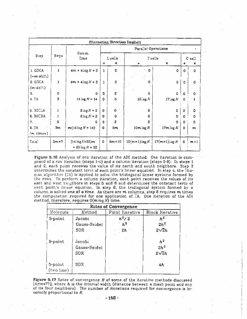
JJternatine, Direction Implicit

ParaJle} Operations

Step Swps Comm. Time L ceJJs T cells C cell

1. GDCA

( -m-shlf:)

2. GDCA

II (m-s'1"::)

3.

i4. TA

15. RO::..A

1

6.RO:CRA

7.

1

0

3

l

l

0

4m + 4logN + 2

4m +4logN+2

0

14 iog N + 14

21ogN + 2

2]ogN + 2

0

... X

l 0

1 0

3 2

0 5

0 0

0 0

3 2

+

o I I

0

0

10]ogN

0

0

0

X +

o o 1

0 0

o I o l7logN j 0

o 1 o

X

0

0

0

I

0

0

0

Is. TA

l(m times) I 3m m(14logN + 14) 0 5m lOmlogN

0

0

l7mlogN

1

m

3m+71

I

(l4logN+22jm

+ 26]ogN + 22 I 0 15m+10 10(m+l)logN 17(m+1)log N o I

I m+l

Figure 5. !6 Analysis of or:e iteratioJO of tl:e AD! method. One iteration is com­posed of a rev; iteraticr: (steps 1-4) and a cch.:mr: iteration (steps 5-8). In steps 1 ar:d 2, each point receives the valt.:e of its north ar:d so10tl: neigl:bors. Step 3 deteroines the cor:stant terr:1 of each point's lir:ear eql..iation. In step 4, the Tha­D~' algcrilr.o (TA) is applied to solve the tridiagcr:al lir:ear systeos formed by the rev.-~. To perfcrr:1 a colt:.r::m iteratim:, each poi~:t receives the values of its east and ·west r:ei;:;:hbors in steps 5 ar:d 6 ar~d deternines the cor_star:t term bf ecct point's lir:ear eqt:.ation. In step 8, U:e tridiagor:.al ·syster:J formed by a coh.=-r:1n is solYed one at a time. As there are m colUI:l.r:.s., step 8 requires m times the ccr:opc.tatior: required for one application of >A. One iteration of the AD! r.1ell:od therefore requires O(m lao A? time . . ~

Rates of Convergence Molecule ! Method Point Iterative Block lterative

5-point 1 Jacobi h 2;2 h2

Gauss-Seidel h2 2h 2

I I SOR 2h 2~h

I I h2 : 9-point Jacobi

! I Gauss-Seidel 2h 2

' I SOR 2~h I I

15-point SOR 4h 1 (t"·o !me)

Figure 5.17 Rates of cor:vergence R of some of the iterative methods discussed [Aoes77], wl:ere his the interval width (distance between a mesh point and ar:y of its four neighbors). The n"t;.mber of iterations required for cor..vergence is in­versely propcrtional to R.

-152-

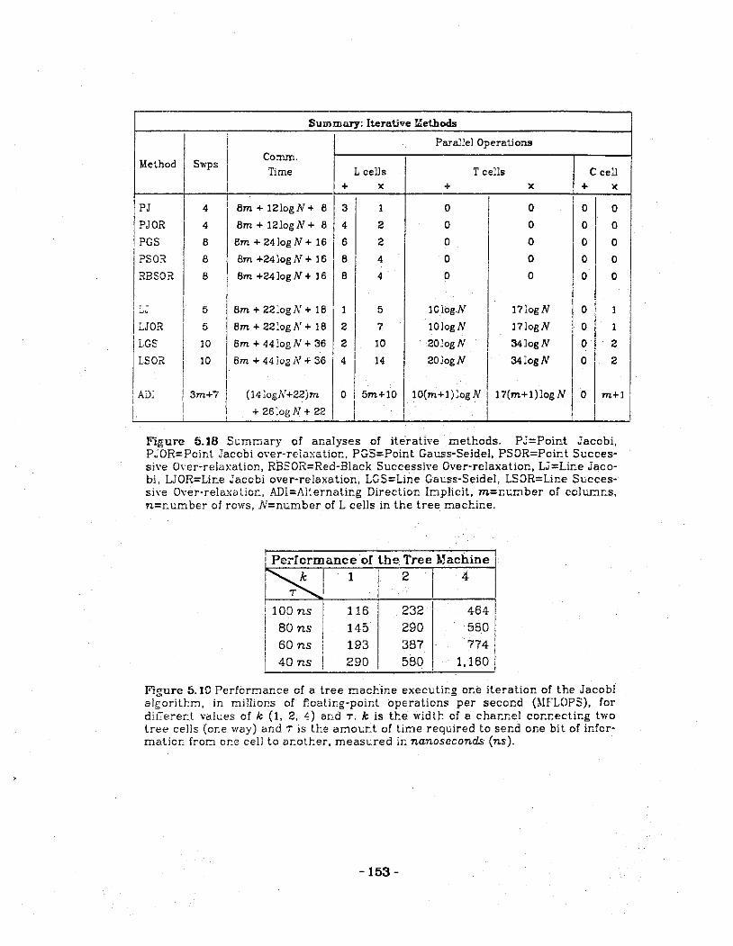
Summary: Iterative Methods

Parallel Opera-tions

Method Sv.-ps Comm. Time L cells T cells C cell

I I+ X + X + X

I

I I I

I PJ I 4 I 8m + 12logN .,_ 8 3 I 0 0 0 0 I

PJOR I 4 8m + 12logN+ 8 4 2 0 0 0 0

PGS I 8 Bm + 24log N + 16 6 2 0 0 0 0

PSO"' I 8 Bm +24logN + 16 8 4 0 0 0 0

RBSOR I

8 8m +24logN + 16 B 4 0 0 0 0

I.,J I 5 Bm + 221ogN + 18 I 5 IGiog.N l7log N 0 I I

I I LJOR

I 5 Bm + 221ogN + 18 2 7

I IOlogN 17logN 0 I

LGS 10 I Bm + 441ogN + 36 2 10 202og N 34logN 0 2 I LSOil 10 IBm+ 44!o.gN + 36 4 14 201ogN 34logN 0 2

I I I m+l I

I I I AD; I 3m+'7 (l4logi\'+22)m 0 5m+IO IO(m+l);ogN 1 17(m+l)logN 0 I

I I I

I i I + 26~ogN + 22 I

' I

Figure 5.18 Sc:mmary of analyses of ite-rative methods. PJ=Point Jacobi, PJOR=Point Jacobi oYer-rela~ation, PGS=Point Gauss-Seidel, PSOR=Pcint Succes­si\'e OYer-relaxation, RBSOR=Red-Black Successi\'e Over-relaxation, LJ=Line jaco­bi, LJOR=Line :acobi over-relaxation, LGS=Line Gacss-Seidel, LSOR=Line Succes­si\'e Over-re1axatior:, ADl=Alternating Direction Ir:1plicit, m=r..t:mber of co1w:J.r..s, n=r:t:.r:Iber of rcws, N=nu.mber of L cells in the tree :machine.

i Pei'Iormance of the Tree Machine

~k ! 1 1 2 4 ! ~I I

100 ns 80ns 60 ns

40ns

116 145 193

290

232 290 387

580

464 580 774

1,160

Figure 5.1C Performance of a tree machine executir:g or..e iteration of the Jacobi algcritbn, in oillioros of floatir:g-point operations per second (MFLOPS), for dif"ererct values of k (1, 2, 4) a10d T. k is tl:e width of a chanr:el com:ectir:g two tree cells (or:e way) and i is lhe amot.;_r:l of tir:1e required to se:r:d one bit of infor­matior: fror::1 or:.e cell to ar:oU:er, meast.:.red ir: nanoseconds (ns).

-153-

CHAPTER 6. CONCLUSION

"\\"e summarize this dissertation by answering the three questions asked in

Chapter 1 and by making several general remarks regarding where one might go

from here.

Can solutions to elliptic partial differential equations be implemented

efficiently on a tree machine? Chapter 5 gave several iterative tree machine

algorithms to solve two dimensional elliptic pde problems. All but one require

O(n) lime to perform one iteration, the ADJ method requires O(nlog n} time.

These compare favorably with the O(n 2) time required on a sequential computer.

The lower complexity of the tree machine algorithms is achieved by efficiently

solving some of the subproblems, such as low-order linear recurrences and

(n x n} tridiagonal linear systems. Linear recurrences (Chapter 3) and tridiago­

nal systems (Chapter 4) can both be solved in O(log n) time. Jn solving the ellip­

tic pde, communication tends to be the costliest part of processing. For exam­

ple, in an (n x n) mesh represented in row major order, the total time required

for each mesh point to communicate with its north and south neighbors is O(n).

Hou; does the tree machine implementation compare u;ith implementations

on other high performance machines. e.g., vector and array processors? Vector

processors can pro,·ide only a constant speedup over sequential computers.

Hence, all of the iterative methods presented in Chapter 5 require O(n 2) time on

a vector processor. On the other hand, an array processor, such as the JLLJAC-

-154-

IV, can implement any of the point iterative methods in constant, i.e .. 0(1) time,

provided there are enough processing elements to store all of the mesh point

values simultaneously. This, of course, is because the interconnection among

the processing elements matches the communication requirements of the mesh

exactly. Consequently, a mesh point (stored in a processing element) can com­

municate with any of its four nearest neighbors in constant time. To implement

a block iterative algorithm or the AD! method, however, requires the solution of

tridiagonal systems. Slone [Slon75] asserts that an (nxn) tridiagonal system

can be solved in O(log n) time on an array processor. A precise description of

communication among the processors, however, was not included in Slone's

analysis. It appears that communication may require O(n) time for the methods

he discusses. If this is the case, then block iterative and AD! methods require

O(n) time on an array processor.

Tree algorithms solving recurrence expressions (Chapter 3) and tridiagonal

linear systems (Chapter 4) compare well with the same algorithms implemented

on vector and array processors. The order of complexity of tree machine algo­

rithms to solve recurrence expressions, O(log n), matches that of array proces­

sors. In all tridiagonal linear system methods studied, the tree algorithms are

consistently better asymptotically than the same algorithms implemented on a

vector processor. In fact, Lamb:otte and Voigt [La Yo75] show that some

me\.hods (direct methods such as Gaussian elimination and LU decomposition,

and iteralive methods such as the Gauss-Seidel and successive over-relaxation)

cannot be implemented efficiently on a vector processor. Moreover, except for

two direct tridia;;onal system solvers (cyclic reduction and the Buneman algo­

rithm), the tr2e al;orilhms match the order of complexity of the best parallel

algorithm kno1·:n for a given problem. This is particularly encouraging because,

-155-

in many instances, what is considered the "best" algorithm is designed for an

idealized parallel processor assuming, for example, that any two processors can

communicate in constant (or even no) time. (Moreover, it should be mentioned

that array processors are snm machines whereas a tree machine can be an

:MJMD computer [Mag679a]. It is beyond the scope of this dissertation to argue

the potential advantages of tree machines over array processors.)

What conclusions regarding tree machine programming do these implemen­

tations provide? Communication among processing elements has emerged as a

primary concern in parallel processing. This is emphasized by Gentleman

[Gent75] who studied the role of data communication in parallel matrix compu­

tations "·hen executed on parallel processors. He showed how communication

among processors, rather than arithmetic operations, can play the dominant

role in the overall performance of an algorithm. Ee cautions against algorithm

analyses that consider only parallel arithmetic operations as they may be very

misleading. (The assumptions in his analysis were such that the conclusions

apply to parallel computation in general, and not just matrix operations.)

The tree algorithms ROTL.4. and GDCA (Chapter 3) have shown that communi­

cation among the L cells of a tree machine need not be restricted to sending all

L cell values up through the root T cell and back down again, i.e., O(N) time

"·here 1\' is the number of L cells. ROTLA and GDCA can often provide communi­

calion in less than linear time. This refutes the often repeated argument tha.t

tree machine algorithms ah,·ays inYolve a bottleneck at the root. By masking

subsets of the 1 cells, ROTLA and GDCA alloO\· a v·ariely of 1 cell communication

patterns.

-156-

Suggestions for Further Work

All methods discussed in this dissertation have been previously developed

and analyzed. No attempt was made to develop new numerical algorithms

specifically suited for a tree machine. A natural extension of this dissertation

would be to develop such methods. Because points are stored among the L cells

in row major order, a mesh point is immediately beside its east and west neigh­

bors but a distance m away from its north and south neighbors. Consequently,

the .total time for all points to communicate with their north and south neigh­

bors is far greater than the total time for all points to communicate "ith their

east and west neighbors. One interesting research topic is the investigation of

numerical algorithms that allow a mesh point to communicate with its north and

south neighbors less frequently than with its east and west neighbors. Is it p.os­

sible lo collect the values of a point's north and south neighbors less frequently

than the values of its east and west neighbors, and still maintain comparable

convergence rates? A related question: is it possible to develop methods that

make good use of asymmetrical molecules? For example, a mesh point may use

the values east of its east neighbor and west of its west neighbor, as well as its

four original neighbors. The values of the two new neighbors can be collected

inexpensively, using ROTRA and ROTLA. The large difference between the time

required by GDCA and by ROTLA motivates further work on these topics.

Another interesting topic is the implementation on a tree machine of a

direct method of solving block-tridiagonal linear systems. Hackney [Eock65,

Hock70] developed a direct method called cyclic reduction, improved by Bune­

man [Bune69] and Buzbee, Golub and Nielson [BuG);70). On a sequential com­

puter, the solution of an (n 2 x n 2 ) block-tridiegonal linear system requires O(n 4 )

-157-

[ChKu75] CHEN, S.C. and KUCK. D.J. Time and parallel processor bounds for linear recurrence systems. IEEE Transactions an Computers C-24, 7 (1975), 701-717.

[ChSa75] CHEN, S.C. and SAMEH, A.H. On parallel triangular system solvers. Proceedings of the 1975 Sagamore Computer Conference an Parallel Processing, (1975), 237-238.

[Chen76] CHEN, S.C. Time and parallel processor bounds for linear recurrence systems "·ith constant coefficients. Jn Proceedings of the 1976 Inter­national Conference an Parallel Processing, P.H. Enslow Jr. (ed.), 196-205.

[ChKS7B] CEE\1, S.C., KUCK. D.J. and SAMEH, A.H. Practical parallel band tri­angular system solvers. ACU Transactions an Mathematical Software 4, 3 (1978), 270-277.

[CoGo73] COl\CUS, P. and GOLUB, G.H. Use of fast direct methods for the efficient numerical solution of nonseparable elliptic equations. SIAM Journal on Numerical Analysis 10, 6 (1973), 1103-1120.

[Co1.iia57] COVEYOU, R.R. and MACPEERSO'\, R.D. Fourier analysis of uniform random number generators. Journal of the ACJ.J 14, 1 (1967), 100-119.

[Diam75] DJAMOl\D, M.A. The stability of a parallel algorithm for the solution of tridiagonal linear systems. Proceedings of the 1975 Sagamore Com­puter Conference on Parallel Processing, (1975), 235.

[DiFe76] DIAMO:\D, M.A. and FERREIRA, D.L. On a cyclic reduction method for the solution of Poisson's equations. SIAlJ Journal on Numerical Analysis 13, 1 (1976), 54-70.

[Dorr70] DORR, F.W. The direct solution of the discrete Poisson equation on a rectangle. SJAJJ Review 12, 2 (1970), 248-263.

[DoRa56] DOl:GL.'\.S, J.Jr. and RACHFORD, H.E.Jr. On the numerical solution of heat conduction problems in two and three space variables. Transac­lbns of the American Mathematical Society 82, (1956), 421-439.

[Doug62] DOVGLAS Jr., J. Alternating direction methods for three space vari­ables . . Numerische Mathematik 4, (1962), 41-63.

[Folia60] FORSYTEE, G.E. and WASOW, W.R. Finite-difference methods for par­tial differential equations, John Wiley & Sons, lnc., New York, 1960.

[Fran79] FRA.\K, G.A. Virtual memory systems for closed applicalive language interpreters. Ph.D. dissertation, Department of Computer Science, Vniversity of Norlh Carolina at Chapel Eill, 1979.

- 160-

[Gajs78] GAJSKI, D.D. Processor array for computing linear recurrence sys­tems. In Proceedings of the 1978 International Conference on Paral­lel Processing, Lipovski, G.J. (ed.), Bellaire, Ml, 1976, 246-256.

[GajsB1] GAJSKI, D.D. An algorithm for solving linear recurrence systems on parallel and pipelined machines. IEEE Transactions an Computers C-30, 4 (1961). 190-206.

[Genl78] GENTLEMAN, W.M. Some complexity results for matrix computations on parallel processors. Journal of the ACM 25, 1 {1976), 112-115.

[HaVa64] HAGEMAN, L.A. and VARGA. R.S. Block iterative methods for cyclically reduced matrix equations. Numerische Mathematik 6, {1964), 106-119.

[Hell74] HELLER, D.E. A determinant theorem with applications to parallel algorithms. SJAJ.f Journal on Numerical Analysis 11. 3 (1974), 559-566.

[Hcll76] HELLER. D.E. Some aspects of the block tridiagonal linear systems. Analysis 13, 4 {1976), 464-496.

cyclic reduction algorithm for SJA.J.f Journal an Numerical

[Hell77] HELLER, D.E. Direct and iterative methods for block-tridiagonal linear systems. Ph.D. dissertatian, Department of Computer Science, Carnegie-Mellon University, April 1977.

[Hell7B] HELLER, D.E. A survey of parallel algorithms in numerical linear alge­bra. SIAM Revie'IL 20, 4 {1976), 740-777.

[HeST76] HELLER. D.E .. STBVB!\SON, D.K. and TRAUB, J.F. Accelerated iterative methods for the solution of tridiagonal systems on parallel comput­ers. Journal of the ACU 23, 4 {1976), 636-654.

[Hoar76] EOARE. C.A.R. Communicating Sequential Processes. Communica­tions of the ACM 21. 6 {1978), 666-677.

[Hock65] HOCKKBY, R.\\'. A fast direct solution of Poisson's equation using Fourier analysis. Jaurnal of the ACM 12, 1 {1965), 95-113.

[Hocl70} EOCE:\I:Y, R.W. The potential calculation and some examples. Methads in Computational Physics 9, Adler, B .. Fernback, S. and Rotenberg. M. {eds.), (1970), 13:>-211.

[HyKu77] HYAFJL, L. and KUKG. H.T. The complexity of parallel evaluation of linear recurrences. Journal of the ACM 24. 3 (1977), 513-521.

[lrHeBO] m;n:\, ~U. ano EELLER, D.E. On-line pipeline systems for recursive numeric comput;:;cions. SJGARCH J\'e'!Lsletter 8, 3 {1980), 292-299.

- 161-

[JeHo79] JESSHOPE, C.R. and HOCKNEY, R.W. (eds.) Super-computers: lnfotech State of the Art Report, Volumes 1 and 2. Jnfotech International Lim­ited, Maidenhead, Berkshire, England, 1979.

[KaMW67] KARP, R.M., MJLLER, R.E. and WINOGRAD, S. The organization of com­putations for uniform recurrence equations. Journal of the ACJJ 14. 3 (1967), 563-590.

[KoSt73] KOGGE, P.M. and STONE, H.S. A parallel algorithm for the efficient solution of a general class of recurrence equations. IEEE Transac­tions an Computers C-22, 8 (1973), 786-793.

[Kogg73] KOGGE, P.M. Maximal rate pipelined solutions to recurrence prob­lems. ln Proceedings of the First Annual Symposium an Computer Architecture, Lipovski, G.J. and Szygenda, S.A. (eds.), Gainesville, FL. 1973, 71-76.

[Kogg74] KOGGE, P.M. Parallel solution of recurrence problems. !BIJ Journal of Research and Development 18, 2 (1974), 138-148.

[Kost77] KOSTER, A. E:<ecution time and storage requirements of reduction language programs on a reduction machine. Ph.D. dissertation, Department of Computer Science, University of North Carolina at Chapel Hill, 1977.

[Kuck75] KUCK. D.J. Parallel processing architecture - a survey. ln Proceed­ings of the 1975 Sagamore Computer Conference an Parallel Process­ing, (1975), 15-39.

[Kuck76] Kl..'CK, D.J. On the speedup and cost of parallel computation. ln The Complexity of Computational Problem Salving, R.S. Anderssen and R.P. Brent (eds.), L'niversity of Queensland Press, St. Lucia, Queens­land, 1976, 63-78.

[Kung76] KUl\G, H. T. New algorithms and lower bounds for the parallel evalua­tion of certain rational expressions and recurrences. Journal of the ACM 23, 2 (1976), 252-261.

[Kung79] KP\G, H.T. Let's design algorithms for VLSJ systems. Report No. CMU-CS-79-151, Carnegie-Mellon University, Pittsburg, PA, 1979.

[KungGO] KUl\G, E.T. The structure of parallel algorithms. Jn Advances in Com­puters 19, E.T. Kung (ed.), Academic Press, i\'ew York, 1980,65-112.

[LaVo75] LAMBJOTTE, J.J. and VOJGT, R.G. The solution of tridiagonal linear sys­tems on the CDC STAR-100 computer. AC\1 Transactions on Mathematical Sof!u;a.rP. 1, 4 (1975), 309-329.

[Leis79] Lr::JSER:OO'\, C. E. Systolic priority queues. Proceedings of the Caltech Conference on VLSJ, (JanCJary 1979), 19~-214.

- 162-

[J.laRo77] MADSEN, N.K. and RODRIGUE, G.H. Odd-even reduction for pentadiag­onal matrices. In Parallel Computers -Parallel Mathematics, M. Feil­meier {ed.), North-Holland Publishing Co., Amsterdam {1977}, 103-106.

[Mag679a] MAGrJ, G.A. A network of microprocessors to execute reduction languages. Two parts. International Journal of Computer and Infor­mation Sciences 8, 5 {1979}, 349-365, and 8, 6 {1979), 435-471.

[Mag679b] MAGrJ, G.A. A cellular, language directed computer architecture. Proceedings of the Caltech Conference on VLSI. {January 1979}, 447-452.

[Mag660] MAGrJ, G.A. A cellular computer architecture for functional program­ming. Spring COMPCON '80. VLSI: New Architectural Horizons, {1960}, 179-165.

[MaSIC61] MAGrJ, G.A., STANAT, D.F. and KOSTER, A. Program execution on a cel­lular computer: some matrix algorithms {In preparation).

[MaPa74] MALCOLM, M.A. and PAL:\IER, J. A fast method for solving a class of tri­diagonal linear systems. Communications of the ACM 17, 1 {1974), 14-17.

[MaRTl6B] MARTIN, R.S., REINSCP., C., and WILKI~SON, J.H. Householder's tridi­agonalization of a symmetric matrix. Numerische Mathematik 11, (1968), 161-195.

[Mira71] MIR-\XKER, W.L. A survey of parallelism in numerical analysis. SIAM Review 13, 4 (1971), 524-547.

[Orcu74] ORCUTT, S. Parallel solution methods for triangular linear systems of equations. Technical Report No. 77, Stanford Electronics Labora­tories, Stanford, CA, 1974.

[OrVo77] ORTEGA, J.M. and VOIGT, R.G. Solution ofpartial differential equations on vector computers. Report No. 77-7, Institute for Computer Appli­cations in Science and Engineering, J\ASA Langley Research Center, Hampton, VA, 1977.

[PeRa55] PEACEMAN, D.W. and RACHFORD, H.H.Jr. The numerical solution of parabolic and elliptic differential equations. Journal of the Society far Industrial and Applied Mathematics 3, 1 (1955), 28-41.

[PoVo74] POOLE Jr., W.G. and VOJGT, R.G. Kumerical algorithms for parallel and vector computers: an annotated bibliography. Computing Reviews 15, 10 (1974), 379-388.

[Poze77] POZEf:OKY, !-.!. Programming in reduction languages. Ph.D. disserta­tion, Depi.lrtment of Computer Science, L'niversity of North Carolina

-163-

at Chapel Hill, 1977.

[PresBl] PRESNELL, H.A. Signal processing algorithms for a reduction machine. Ph.D. dissertation in preparation, Department of Computer Science, University of North Carolina at Chapel Hill.

[PrPaBl] PRES:!\ELL, H.A. and PARGAS, R.P Communication along shortest paths in a tree machine. Proceedings of the Conference on Functional Pro­gramming Languages and Computer Architecture, Portsmouth, 1981, 107-114.

[Rice79) RJCE, J.R., GEAR, C.W., ORTBGA, J., PARLETT. B., SCHULTZ, M., SHAM­Pl:!\E, L.F., WOLFE, P. and TRAUB, J.F. (edE.} Kumerical computation: its nature and research directions. ACJ.J SJGNG'M Newsletter Special Issue, (February 1979).

[Rofi::K79] RODRJGUE, G.H., MADSEN, N.K. and K-'I.RUSH, J.l. Odd-even reduction for banded linear equations. Journal of the ACJ.J 26, 1 (1979), 72-81.

[Same71] SAMEH, A.H. On Jacobi and Jacobi-like algorithms for a parallel com­puter. Mathematics of Computation 25, 115 (1971}, 579-590.

[SaBr77] SA.MEE, A.H. and BRENT, R.P. Solving triangular systems on a parallel computer. SIAN Journal of Numerical Analysis 14, 6 (1977}, 1101-1113.

[SaKu77] SA.lvfEH, A.H. and KUCK, D.J. Parallel direct linear system solvers - a survey. ln Parallel Computers - Parallel Nathematics, M. Feilmeier (ed.}, North-Holland Publishing Co., Amsterdam (1977), 25-30.

[SaKu7B] SAMEH, A.H. and KUCK, D.J. On stable parallel linear system solvers. Journal of the ACM 25, 1 (1978}, 81-91.

[SchuB1] SCEULTZ, M. Elliptic Problem Solvers, Academic Press, New York, 1981.

[Slon73a] STO\E, H.S. An efficient parallel algorithm for the solution of a tridi­agonal linear system of equations. Journal of the ACM 20, 1 (1973}, 27-38.

[Ston73b] STOKE, E.S. Problems of parallel computation. ln Complexity of sequential and parallel numerical algorithms, J.F. Traub (ed.}, Academic Press, New York (1973}, 1-16.

[Slon75] STOC\E, H.S. Parallel tridiagonal equation solvers. ACM Transactions on Mathematical Software 1, 4 (1975}, 289-307.

[Ston76] STO\E, H.S. Computer architedure in the 1980s. In Computer Sci­£nce a_nd Sci~ntific Comp?..!Ji';l,g, J.~ .. L Ortegr.. (ed.), Academic Press, 1\ev,· York (1976), 127-153.

- 164-

[S>.ar74u] SWARZTRAUBER. P.l\. A direct method for the discrete solution of separable elliptic equations. SIAM Journal on Numerical Analysis 11. 6 (1974), 113G-1150.

[S\7ar74b] S\IARZTRAt;BER, P.l\. The direct solution of the discrete Poisson equation on the surface of a sphere. Journal of Computational Phy­sics 15, 1 (1974), 46-54.

[Sr.ar7B] SYiARZTRAUBER, P.l\. A parallel algorithm for solving general tridiag­onal equations. J.!athematics of Computati~n 33, 145 (1979), 185-199.

[Sro3"1773] SYiARZTRAUBER. P.N. and S\YEET, R.A. The direct solution of the discrete Poisson equation on a disk. SJA.!.J Journal on Numerical Analysis 10, 5 (1973), 900-907.

(S\7ee73] SY;EET, R.A. Direct methods for the solution of Poisson's equation on a staggered grid. Journal of Computational Physics 12, 3 (1973), 422-428.

[&.ee74] SYiEET, R.A. A ;;eneralized cyclic reduction algorithm. SJAU Journal on ]\'umeri~alAnalysis 11, 3 (1974), 506-520.

[TolHll] TOLLE, D.:\!. Coordination of computation in a binary tree of proces-. sors: an archilectural proposal. Ph.D. dissertation, Department of Computer Science, University of Korth Carolina at Chapel Eill, 1981.

[ToSiSl] TOLLE, D.M. and SJDDALL, \\'.E. On the complexity of vector computa­tions in binary tree machines. Jnformati~n Processing Letters 13, 3 (1951), 120-124.

[Trau73] TRA"LB, J.F. Iterative solution of tridiz.gonal systems on parallel and vector computers. ln CoTT.pLcxi!y of Sequential and Parallel Numeri­cal Algorithms, J.F. Traub (ed,), Academic Press, Xew York, 1973, 49-82.

[Vara72] \'ARAE, .J.1!. On lhe E<:>lulion of block-tridiagonal systems arising from ceclie.in finite-difference equations . • ~:azh,.matics of Computation 26, 120 ( 19-r2). 858-588.

[Vart;CZ] \'ARGA, R.S. J.h.tri.x iteratiJ;g numsrical analysis, Wiley, Kew York, 1902.

[r:c.Jl~SJ \\".'..11. E.S. /;1:aoyiic Theory of Coniinued Fractions, \'an Xostrand, ~\cv; York, 19..;.9.

[f,'ill61] Y;iLLlA\:S Jr .. I:.n. Anillysis of FFP programs for parallel associative scc.rcbi:lz. Fi1.D. di.s~2r~~~ian. D::;;:,D.rLITieJ!t of Compuler Science, Lnh·crsl~:: c; \::.:-L~: C~Fo~:~J.. ~t Ch~~·el Eill, 18fH.

[Ym .. :n7"1] :.·oL·\,:;, D.l~~- li2~·-::.U1:~ s~l11.tia~<. af lcr.~·ge li.r:~2r sy:;tems, Academic Press, Kew York, 1971.

- 165-