
Dejavu:An accurate Energy-Efficient Outdoor Localization System SIGSPATIAL '13.

Towards an Efficient and Accurate Schedulability Analysis for Real-Time Cyber-Physical Systems
Mitra Nasri
Assistant professorDelft University of Technology
2
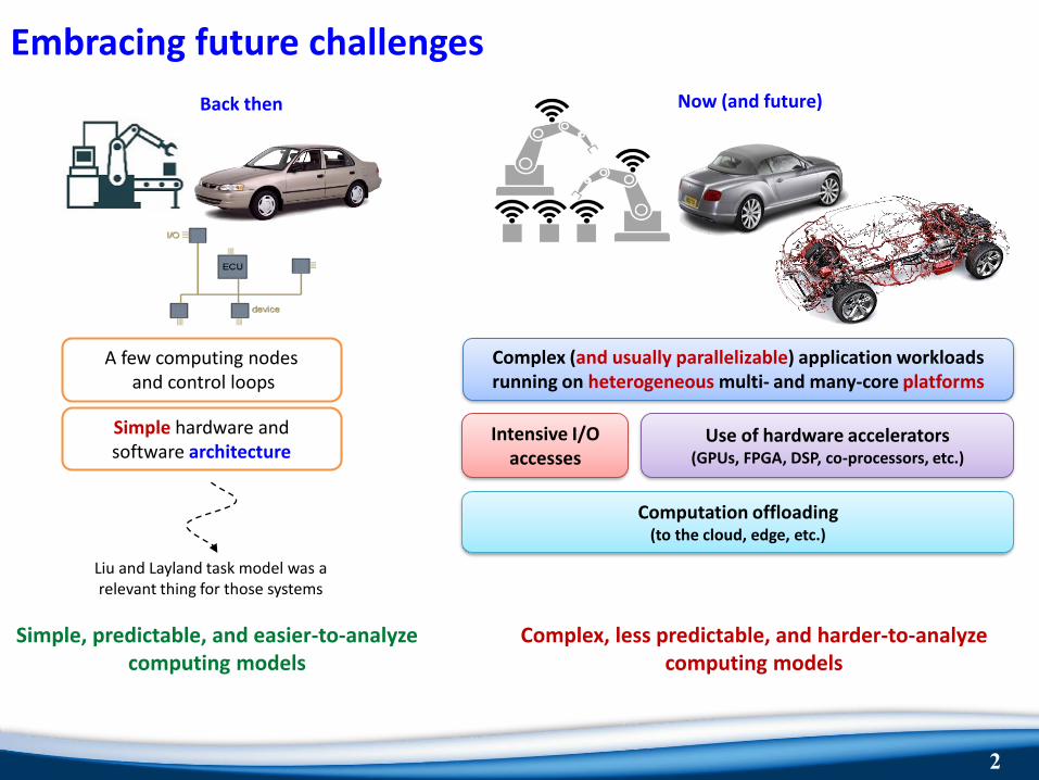
Now (and future)
Simple hardware and software architecture
Embracing future challenges
A few computing nodesand control loops
Intensive I/O accesses
Complex (and usually parallelizable) application workloads running on heterogeneous multi- and many-core platforms
Use of hardware accelerators (GPUs, FPGA, DSP, co-processors, etc.)
Computation offloading (to the cloud, edge, etc.)
Complex, less predictable, and harder-to-analyze computing models
Simple, predictable, and easier-to-analyzecomputing models
Back then
Liu and Layland task model was a relevant thing for those systems

3
A wish list
Bounded or unboundeduncertainty
time
deadline
Arrival modelTask precedence
Machine 2Machine 1
Network
Execution model
Parallel heterogeneous DAG tasks with conditional branches
resource affinity
• Each resource may have its own scheduling policy• Schedulers may have different runtime overheads
bounded uncertainty
AND
OR
suspension
Obtain the worst-case and best-case response time
Occupation time of a resource

4
State of the art
4
Closed-form analyses (e.g., problem-window analysis)
• Fast • Pessimistic• Hard to extend
0
0.2
0.4
0.6
0.8
1
0.1 0.2 0.3 0.4 0.5 0.6 0.7 0.8
sch
edu
lab
ility
rat
io
utilization
M. Serrano, A. Melani, S. Kehr, M. Bertogna, and E. Quiñones, “An Analysis of Lazy and Eager Limited Preemption Approaches under DAG-Based Global Fixed Priority Scheduling”, ISORC, 2017.
[Serrano’17]
[Nasri’19]
Experiment:10 limited-preemptive parallel DAG tasks scheduled by global FP on 16 cores
Non-problem-window based solution
Mitra Nasri, Geoffrey Nelissen, and Björn B. Brandenburg, "Response-Time Analysis of Limited-Preemptive Parallel DAG Tasks under Global Scheduling", the Euromicro Conference on Real-Time Systems (ECRTS), 2019, pp. 21:1-21:23.

5
State of the art
Closed-form analyses (e.g., problem-window analysis)
• Fast • Pessimistic• Hard to extend
Exact tests in generic formal verification tools (e.g., UPPAAL)
• Accurate• Easy to extend
• Not scalable
The “tool” does all the labor (to find the worst case)
Generic verification tools are very slow and do not scale to reasonable problem sizes

6
0.00
0.25
0.50
0.75
1.00
3 6 9 12 15 18 21 24 27
sch
edu
lab
ility
rat
io
number of tasks
4 cores, 30% utilization
exact test (timeout)
this paper
exact test (UPPAAL)
[Nasri’19]
Results from formal verification-based analyses
0
500
1,000
1,500
2,000
2,500
3,000
3 6 9 12 15 18 21 24 27 30 33 36 39 42 45 48 51 54 57 60
run
tim
e (s
ec)
number of tasks
8 cores
4 cores
2 cores
1 core[Nasri’19](8 cores)
Sequential non-preemptive periodic tasks (scheduled by global FP)

7
State of the art
7
Closed-form analyses (e.g., problem-window analysis)
• Fast • Pessimistic• Hard to extend
Exact tests in generic formal verification tools (e.g., UPPAAL)
• Accurate• Easy to extend
• Not scalable
Our new line of work
Idea: efficiently explore the space of all possible
schedules • Applicable to complex problems• Easy to extend • Highly accurate• Relatively fast
Response-time analysis using schedule abstraction

8
0
0.2
0.4
0.6
0.8
1
0.1 0.2 0.3 0.4 0.5 0.6 0.7 0.8
sch
edu
lab
ility
rat
io
utilization
this paper (m=4) Serrano (m=4)
10 parallel random DAG tasksSome results on parallel DAG tasks
M. Serrano, A. Melani, S. Kehr, M. Bertogna, and E. Quiñones, “An Analysis of Lazy and Eager Limited Preemption Approaches under DAG-Based Global Fixed Priority Scheduling”, ISORC, 2017.
0
0.2
0.4
0.6
0.8
1
0.1 0.2 0.3 0.4 0.5 0.6 0.7 0.8
sch
edu
lab
ility
rat
io
utilization
this paper (m=8) Serrano (m=8)
0
0.2
0.4
0.6
0.8
1
0.1 0.2 0.3 0.4 0.5 0.6 0.7 0.8
sch
edu
lab
ility
rat
io
utilization
this paper (m=16) Serrano (m=16)
39
294
418
0
100
200
300
m=4 m=8 m=16
run
tim
e (
s)
average0.90 percentile0.95 percentile0.98 percentile
[ECRTS’19] (m=4) [ECRTS’19] (m=8)
[ECRTS’19] (m=16)

99
Response-time analysis using schedule abstraction

10
An example: the problem of global non-preemptive scheduling
Global job-level fixed-priority (JLFP)
Scheduler model
Multicore (identical cores)
Platform model
Obtain the worst-case and best-case response time
Workload model
Non-preemptive job sets
Release jitterDeadline
Job model𝐽1
Deadline
𝐽2
…The job set is provided for an observation window, e.g., a hyperperiod.
This job model supports bounded non-deterministic arrivals, but not sporadic tasks (un-bounded non-deterministic arrivals)
Execution time variation

11
Solution highlights
Use job-ordering abstraction to analyze schedulability by building a graph that represents all possible schedules
Solution
There are fewer permissible job orderings than schedules
Observation
A sound analysis must consider all possible execution scenarios
(i.e., combination of release times and execution times)
Due to scheduling anomalies

12
A path represents a set of similar schedules
Different paths have different job orders
Response-time analysis using schedule-abstraction graphs
start end
A path aggregates all schedules with the same job ordering

13
Response-time analysis using schedule-abstraction graphs
Earliest and latest finish time of 𝐽1when it is dispatched after state 𝑣
start end
A path aggregates all schedules with the same job ordering
A vertex abstracts a system state and an edge represents a dispatched job
𝑱𝟏:[4, 8]𝑣

14
Response-time analysis using schedule-abstraction graphs
Core 1:Core 2:
10 30
15 20
A system state
Interpretation of an uncertainty interval:
Possibly available
Certainly not available
Certainly available
start end
A path aggregates all schedules with the same job ordering
A vertex abstracts a system state and an edge represents a dispatched job
A state is labeled with the finish-time interval of
any path reaching the state
10 30

15
Earliest and latest completion times of the job in the path
Obtaining the response time:
Response-time analysis using schedule-abstraction graphs
𝑱𝟏: [2, 5]
𝑱𝟏:[4, 8]𝑱𝟏: [7, 15]
Best-case response time = min {completion times of the job} = 2Worst-case response time = max {completion times of the job} = 15
A path aggregates all schedules with the same job ordering
A vertex abstracts a system state and an edge represents a dispatched job
A state represents the finish-time interval of
any path reaching that state

16
Initial state
merged
merged
merged
merged
Building the schedule-abstraction graph
Building the graph (a breadth-first method)
Repeat until every path includes all jobs1. Find the shortest path 2. For each not-yet-dispatched job that can be dispatched after the path:
2.1. Expand (add a new vertex)
2.2. Merge (if possible, merge the new vertex with an existing vertex)
System is idle and
no job has been scheduled

17
Building the schedule-abstraction graph
Expansion rules imply the scheduling policy
Core 1:Core 2:
10 30
15 20
State 𝒗𝒊Next states
J1
J2
8 25J2 Medium priority
17 30J1 High priorityAvailable jobs
(at the state)
35 40J3 Low priority
Expanding a vertex: (reasoning on uncertainty intervals)
𝑣𝑖

18
Define the state abstraction
Define the expansion rules
Define merging rules
How to use schedule-abstraction graphs to solve a new problem?
What is encoded by an edge?What is encoded by a state?
How to create new states?
How to identify similar states?
And then, prove soundness“the expansion rules must cover all possible schedules of the job set”

19
Challenges
https://www.globallanguageservices.co.uk/30-days-of-language-challenges/

20
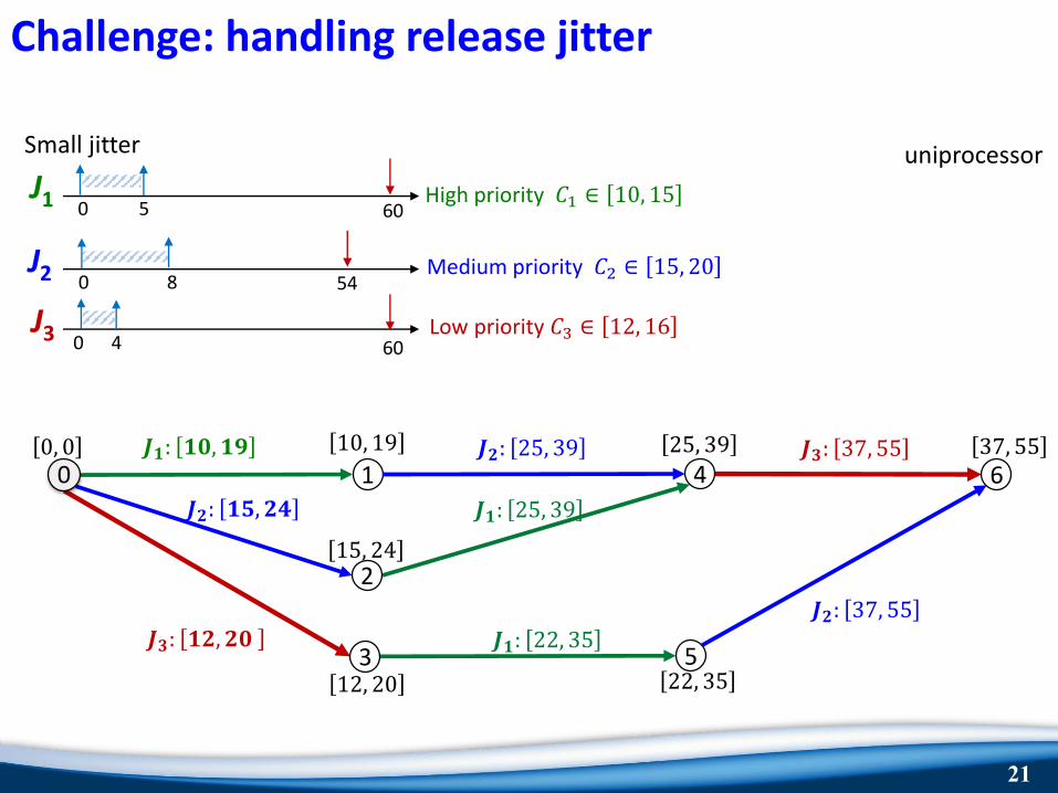
Challenge: handling release jitter
0 J2 Medium priority 𝐶2 ∈ 15, 20
0 J1 High priority 𝐶1 ∈ 10, 15
0 J3 Low priority 𝐶3 ∈ 12, 16
54
60
60
1𝑱𝟏: 𝟏𝟎, 𝟏𝟓
10, 15 𝑱𝟐: 25, 35 25, 35
2𝑱𝟑: 37, 51 37, 51
3
00, 0
No jitter uniprocessor
21
Challenge: handling release jitter
𝑱𝟏: 25, 39
𝑱𝟐: 37, 55
1𝑱𝟏: 𝟏𝟎, 𝟏𝟗 10, 19
𝑱𝟐: 𝟏𝟓, 𝟐𝟒
15, 242
𝑱𝟑: 𝟏𝟐, 𝟐𝟎
12, 203
𝑱𝟏: 22, 35
22, 355
𝑱𝟐: 25, 39 25, 39
4𝑱𝟑: 37, 55 37, 55
6
0 8J2 Medium priority 𝐶2 ∈ 15, 20
0 5J1 High priority 𝐶1 ∈ 10, 15
0 4J3 Low priority 𝐶3 ∈ 12, 16
54
60
60
00, 0
Small jitter uniprocessor

22
Challenge: handling release jitter
𝑱𝟏
1𝑱𝟏
𝑱𝟐
2𝑱𝟑
3
𝑱𝟏
𝑱𝟐4
𝑱𝟑7
0 30J2 Medium priority 𝐶2 ∈ 15, 20
0 35J1 High priority 𝐶1 ∈ 10, 15
0 40J3 Low priority 𝐶3 ∈ 12, 16
54
60
600
𝑱𝟑5
Larger jitter
6𝑱𝟑
𝑱𝟐
𝑱𝟐
𝑱𝟏
The maximum number of branches follows the binomial co-efficient
uniprocessor
Large release jitter (or sporadic release) may result in a combinatorial state space

23
Challenge: handling release jitter
Partial-order reduction
Potential solutions
Avoid exploring paths that do not contribute to the worst-case scenario.
Use approximation to derive the worst-case completion time of the
remaining jobs in that path
Large release jitter (or sporadic release) may result in a combinatorial state space

24
Challenges: handling release jitterLarge release jitter may result in a combinatorial state space
Partial-order reduction
Potential solutions
Derive expansion rules for a set of jobs
Batch processing (rather than processing a single job at a time)
1𝑱𝟏, 𝑱𝟐
𝑱𝟐, 𝑱𝟑2
3
4
0𝑱𝟏, 𝑱𝟐, 𝑱𝟑
𝑱𝟑
𝑱𝟏
{ }
J2 Medium
J1 High
J3 Low
J4 Highest
priority 𝑱𝟒 𝑱𝟑1
𝑱𝟏, 𝑱𝟐
𝑱𝟐, 𝑱𝟑
2
3
4
0
𝑱𝟏, 𝑱𝟐, 𝑱𝟑
𝑱𝟒
{𝑱𝟒}
7
5
6
𝑱𝟏
{ }

25
Challenges: handling release jitterLarge release jitter may result in a combinatorial state space
Partial-order reduction
Potential solutions
Batch processingUsing memorization
(to avoid exploring previously seen patterns)
What else?
Thank you.