Towards a Property PreservingTransformation from IEC 61131–3 to BIP

Jan Olaf Blech, Anton Hattendorf, Jia Huangfortiss GmbH, Guerickestraße 25, 80805 Munchen, Germany

August 28, 2018

Abstract We report on a transformation from Sequential Function Charts of the IEC61131–3 standard to bip. Our presentation features a description of formal syntax andsemantics representation of the involved languages and transformation rules. Further-more, we present a formalism for describing invariants of IEC 61131–3 systems andestablish a notion of invariant preservation between the two languages. For a subset ofour transformation rules we sketch a proof showing invariant preservation during thetransformation of IEC 61131–3 to bip and vice versa.

This work has been supported in part by the European research project ACROSS under the Grant

Agreement ARTEMIS-2009-1-100208.

1 Introduction

In this paper we provide a formal definition of a subset of the Sequential Function Chart(SFC) language from the IEC 61131–3 standard and the bip language. The IEC 61131–3standard [19] describes languages widely used in the industrial control domain to writeprograms for programmable logic controllers (PLC). bip [4] is a language to describecomponent based systems. It is based on state transitions that are encapsulated intocomponents. These components are connected with each other. Via connectors they caninteract and synchronize.

We contribute a transformation specification from SFCs into bip. This transformationis designed to preserve the behavior of SFCs while using as much of bips parallelism aspossible.

We also present a description for invariants in the SFC language and show how in-variants from bip can be transformed into SFC invariants and vice versa. A proof thatinvariant properties discovered on bip do also hold for the original SFCs is provided toshow that the transformations are correct.

1

arX

iv:1

009.

0817

v1 [

cs.P

L]

4 S

ep 2

010

1.1 Related Approaches

Formal specification and correctness of model to model transformations have been ex-tensively studied in the context of graph-transformations [13]. Our work, however, hasbeen stronger influenced by approaches to guarantee the correctness or distinct proper-ties of compiler runs (e.g., [18, 15, 17]). Our transformation rules for the IEC 61131–3to bip transformation can be regarded as the definition for a compiler. Guaranteeingcorrectness of our transformation by using translation validation like techniques is a longterm goal of our work. This could be similar to [6].

The issue of property preservation has been studied in [16]: The work comprisesconditions and a proof that under these conditions abstractions preserve temporal logicsproperties. Our transformations may be regarded as abstractions. The invariant basedsafety properties studied in this paper are a simple (but yet powerful) case of theseproperties.

Various other bip transformations exist that are relevant for our work. Most notablysynchronous bip [11] is a language subset of bip that is especially suitable for the trans-formation of synchronous languages into bip. The languages of IEC 61131–3 are alsosynchronous. Furthermore the translation from AADL to bip has been studied [12]. Coqcertificates guaranteeing correct invariants for bip have been studied in [8].

1.2 Lifting Safety Properties Through a Transformation Chain

On a general level we are interested in transformation chains where models get trans-formed into other models and finally into machine code. Some analysis tool might beinvoked on one of these representations. In particular we are interested in analyses thatdiscover system invariants on one of the intermediate models. Safety results may bederived from the analysis of such an invariant.

We are interested in lifting such invariants and connected safety results from onerepresentation to another. In particular we are interested in two different use-cases.

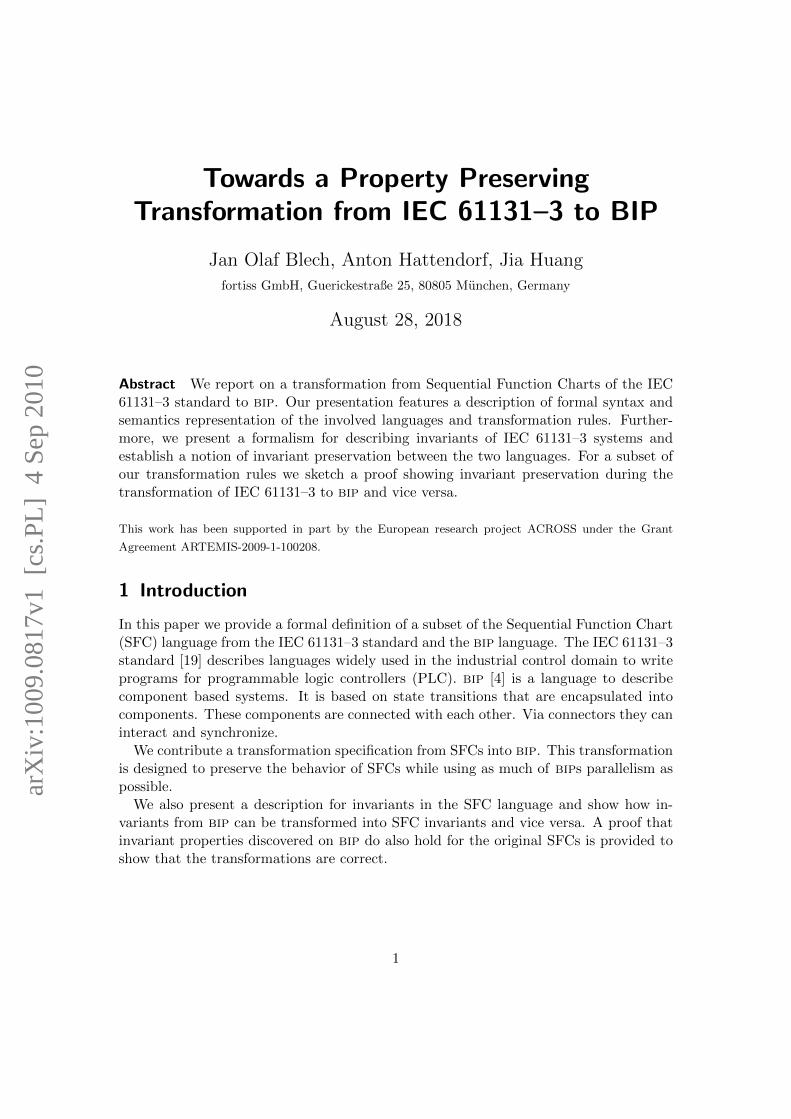
Use-Case 1: Lifting Invariants and Safety Properties to an Earlier Stage in theModel Transformation Chain This comprises the lifting of invariants and connectedsafety properties to the beginning of a chain of model to model transformations (cf.Figure 1), i.e., transforming model’ to model and then invariant’ to invariant. This canbe done if the following conditions are fulfilled:

• Models at an earlier stage in the transformation chain allow at least as muchbehavior as models at the analysis stage in the transformation chain.

• Invariants at the analysis stage are at most as strong as corresponding invariantsat earlier stages in the transformation chain.

The fact that invariants may only get stronger when transforming them for an earliermodel representation ensures the preservation of safety properties. However, we have toshow invariant preservation:

2

⊆model

...

...

model’

Transformations

model”

invariant invariant’⊆ ⊆

⊇ ⊇

safety propertysafety property

⊇ ⊇

Transformations

...⊆

Figure 1: Use-Case 1

• We have to show that for each concrete transformation invariant is indeed an in-variant of model.

Correctness of model and invariant transformation can be formally stated in the followingway. Given a (model to model) transformation function TS and an invariant transforma-tion function TI : for every system model there is a transformation model′ = TS(model), ifwe have discovered an invariant invariant′ for model′ (denoted model′ |= invariant′) thenthere exists an invariant invariant = TI(invariant′) such that model |= invariant. If Tipreserves safety properties, this ensures that safety properties discovered by analyzingI2 do also hold for the original system model.

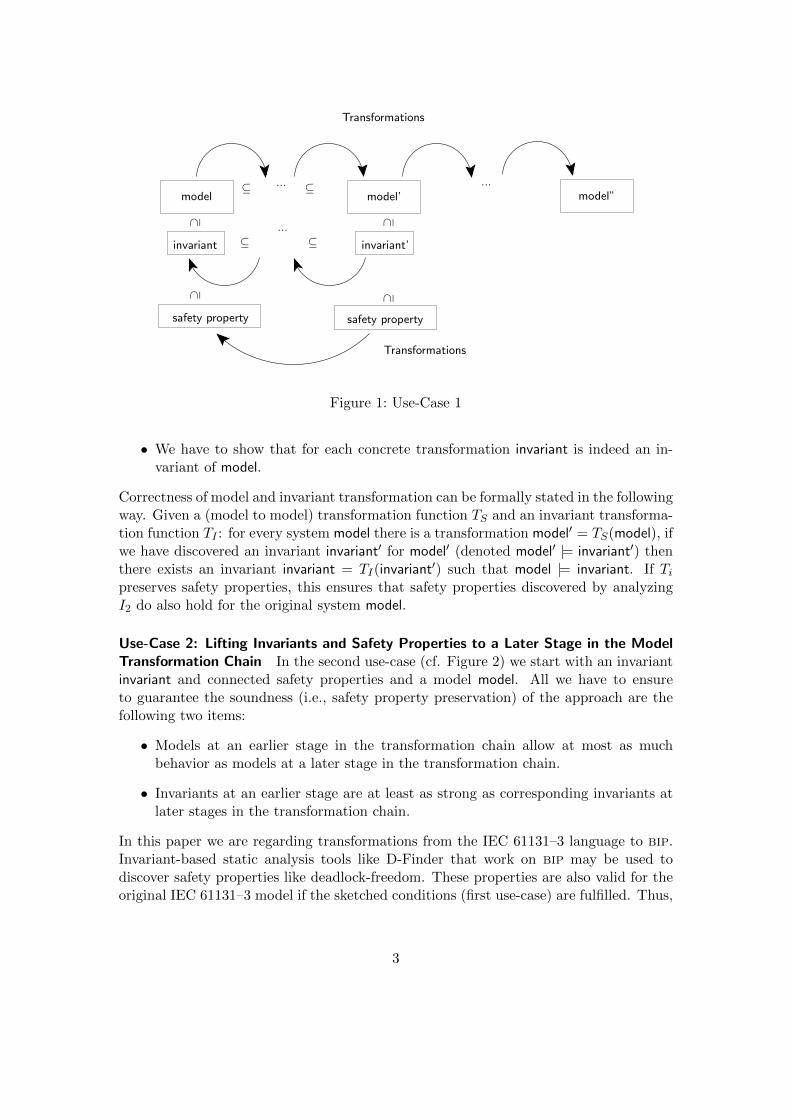
Use-Case 2: Lifting Invariants and Safety Properties to a Later Stage in the ModelTransformation Chain In the second use-case (cf. Figure 2) we start with an invariantinvariant and connected safety properties and a model model. All we have to ensureto guarantee the soundness (i.e., safety property preservation) of the approach are thefollowing two items:

• Models at an earlier stage in the transformation chain allow at most as muchbehavior as models at a later stage in the transformation chain.

• Invariants at an earlier stage are at least as strong as corresponding invariants atlater stages in the transformation chain.

In this paper we are regarding transformations from the IEC 61131–3 language to bip.Invariant-based static analysis tools like D-Finder that work on bip may be used todiscover safety properties like deadlock-freedom. These properties are also valid for theoriginal IEC 61131–3 model if the sketched conditions (first use-case) are fulfilled. Thus,

3

⊇model

...

...

model’

Transformations

...

...

model”⊇

invariant invariant’ ⊆

⊇

⊆ invariant”⊆ ⊆

⊇ ⊇ ⊇

safety propertysafety property

⊇ ⊇

Transformations

safety property

⊇

⊇

Figure 2: Use-Case 2

if we have a trustable code-generation from IEC 61131–3 models and do trust D-Finder,we can use this code generation to generate code that we can trust to be deadlock-free given a successful D-Finder run. The other application corresponds to the seconduse-case: Lifting safety properties and connected invariants from IEC 61131–3 to bip.

1.3 Overview

We define a formal semantics of the Sequential Flow Chart part of the IEC 61131–3standard in Section 2. A summary of the bip language and its semantics is given inSection 3. The transformation from this language into bip is described in Section 4.Invariant preservation from bip back to the SFC language is discussed in Section 5.The other direction: invariant preservation from SFCs to bip is presented in Section 6.Finally, Section 7 features a conclusion.

2 The SFC Language and a Formal Definition of its Semantics

This section presents an overview on the Sequential Function Charts (SFC) languageand a formal definition of SFC including the operational semantics. This formulation isbased on the IEC 61131-3 standard [19] and existing work [3, 9, 10]. We are particularlyinterested in the subset of IEC 61131–3 that is used in the EasyLab toolkit [2].

2.1 A Formal Definition of the SFC Syntax

SFC is one of the graphical programming languages described in the IEC 61131-3 stan-dard. It comprises control locations of the system (called steps) and the transition ofcontrol between them. The passing of control can be restricted via guards. Behaviors

4

of the program is described in action blocks which can be associated with steps. In thefollowing, we first define the basic component of SFCs and then describe the composi-tion of them. We define in fact two formal descriptions of the SFC language. One thatsupports the subset used by the Easylab toolkit and an extended version that supportsmore features described in the standard.

Variables in the SFC Language SFCs have variables that are visible to all their com-ponents, such as steps, guards and actions. We use X = x1, x2, ..., xn to denote the setof variables. The current values of X are described using a variable valuation function(usually denoted f in the context of this paper) of type X → valX , which assigns avalue compatible to the respective data type (valX) to each variable in X. We use F todenote the set of all valuation functions of X.

Action Blocks and Steps (Extended) action blocks and steps in SFCs are the basicunits for describing the behavior.

Definition 1 (Actions) An action is an update function of type F → F .

The definition of actions is the same for extended and non-extended SFCs.

Definition 2 ((Extended) Action block) For a given set of actions A an extendedaction block is a tuple (a, q), where– a is the action, which can be either an update function of type F → F ∈ A or anidentifier to a nested SFC, and– q is a qualifier q ∈ N,S,R, P0, P1, the semantics of which are introduced shortly.

A non-extended action block comprises just an update function of type F → F . Inthis case, the term action block and update function may be used synonymously.

The same action can be used in multiple action blocks associated with different SFCsteps. In IEC 61131–3 the update functions can be written in any other languages definedin the standard, such as Function Block Diagram (FBD), Structured Text (ST), LadderDiagram (LD) and Instruction List (IL). Here we abstract from a concrete language anduse mathematical functions instead.

The action block qualifiers describe the activity of actions. The semantics of thequalifiers are defined as follows:

• N (non-stored) qualifier describe actions that are active only when parent stepsare activated,

• S (stored) qualifier describe actions that continue being active until a reset actionis executed,

• R (stored) actions are used for reseting active actions,

• P0 (pulse at falling edge) actions are active only when the parent step is exited,

5

• P1 (pulse at rising edge) actions are active only when the parent step are entered.

The reset actions tagged with R have always the highest priority.

Definition 3 (Step) For a given set of action blocks B and its associated set of actionsA. A step of an SFC is a pair s = (n,Ω), where n is a unique identifer for the step andΩ = 2B (note that B = A for the non-extended case) is a set of action blocks belongingto the step. We use s.Ω to refer to the set of action blocks associated with step s.

The steps can be in inactive, ready or active state. An inactive step does not activateany actions. The ready steps are the ones that control resides in. However, it is notnecessary that the actions of ready steps will be performed. A special situation is innested SFCs, where a step in a nested SFC is ready but the parent action is not active.In this case, the actions of ready steps will not be performed. The active steps are thoseready steps whose actions will actually be performed.

Guards and Transitions Steps in SFCs are connected via transitions. Transitions fea-ture a guard expression.

Definition 4 (Guard) A guard g is a predicate over a valuation function. It has thetype g : F → bool, where F is the set of all valuation functions. It evaluates to true ifthe current values of X satisfy g.

Definition 5 (Transition) A transition t ∈ T = (tsrc, tg, ttgt) describes the moving ofcontrol from source steps tsrc to target steps ttgt. A transition is enabled if the guard tgevaluates to true. A transition is taken if no conflicting transition with higher priorityis enabled.

SFC Definition The definition of SFCs is the same for both extended and non-extendedSFCs. However, the set of actions has a different type.

Definition 6 (SFC) An SFC is a 7-tuple S = (X,A, S, S0, T,@,≺), where

• X is a finite set of variables,

• A a finite set of actions,

• S is a finite set of steps, comprising action blocks which depend on A (in case ofnon-extended SFCs are equal to A)

• S0 is the set of initial steps,

• T ⊆ (2S\∅)×G× (2S\∅) is the set of transitions, where G is the set of guards,

• @∈ A× A is a total order on actions used to define the order in which the activeactions are to be executed, and

• ≺∈ T × T is a partial order on transitions to determine the priority on conflictingtransitions.

6

S1 x=x+1;a1

x=x-1;a2

y=x;a3

S2

a1

a1a3

S3 a2a3

S4

x<10 x>10

true

t1 t2

t3 t4

t5

x>15 x<5

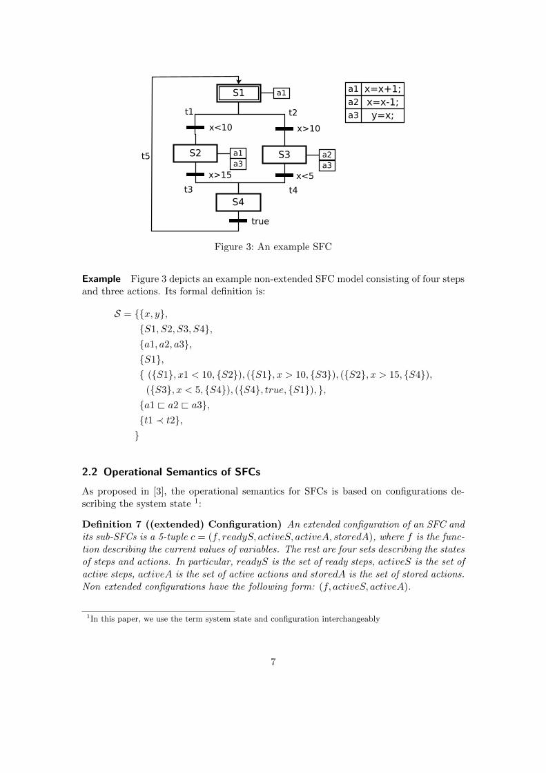
Figure 3: An example SFC

Example Figure 3 depicts an example non-extended SFC model consisting of four stepsand three actions. Its formal definition is:

S = x, y,S1, S2, S3, S4,a1, a2, a3,S1, (S1, x1 < 10, S2), (S1, x > 10, S3), (S2, x > 15, S4),

(S3, x < 5, S4), (S4, true, S1), ,a1 @ a2 @ a3,t1 ≺ t2,

2.2 Operational Semantics of SFCs

As proposed in [3], the operational semantics for SFCs is based on configurations de-scribing the system state 1:

Definition 7 ((extended) Configuration) An extended configuration of an SFC andits sub-SFCs is a 5-tuple c = (f, readyS, activeS, activeA, storedA), where f is the func-tion describing the current values of variables. The rest are four sets describing the statesof steps and actions. In particular, readyS is the set of ready steps, activeS is the set ofactive steps, activeA is the set of active actions and storedA is the set of stored actions.Non extended configurations have the following form: (f, activeS, activeA).

1In this paper, we use the term system state and configuration interchangeably

7

Semantics of Extended SFCs Execution of one SFC-cycle consists of the followingthree phases:

• Phase 1: execute actions contained in set activeA and update the values of variablescorrespondingly;

• Phase 2: perform step transitions and update the sets readyS, activeS;

• Phase 3: compute the set of active/stored actions activeA and storedA for thenext cycle.

In each of the three phase, the configuration of the SFC system is updated. Thesemantics of an SFC can then be regarded as a transition system of the configurations.

Definition 8 (Transition system of an extended SFC) An extended SFC

S = (X,A, S, S0, T,@,≺)

is associated with a transition system E(S) = (C, c0,→), where C is the set of configura-tions, c0 is the initial configuration and →⊆ C × C is the transition relation.

Elements in the transition relation for extended SFCs have the following form:

(f, readyS, activeS, activeA, storedA)→ (f ′, readyS′, activeS′, activeA′, storedA′)

The details of the transition relation are described as follows:

• In Phase 1, f ′ is updated by performing the set of active actions, which are executedaccording to the orders specified in @, that is, f ′ = (am ... a1)(f), wherea1 @ ... @ am and a1, ..., am are the set of active update functions. The rest ofthe configuration remains unmodified.

• In Phase 2, readyS, activeS are updated and the rest of the configuration remainsthe same. readyS′ is obtained by evaluating transitions T . Let c be the currentconfiguration, the set of transitions that can be taken can be identified as T =t = (tsrc, tg, ttgt) ∈ T | tsrc ⊆ activeS ∧ c |= tg ∧ (¬∃t′ . t′src ⊆ activeS ∧ c |=g′∧ tsrc∩ t′src 6= ∅∧ t ≺ t′), that is, a transition is taken if its guard is satisfied andthe conflicting transitions, which are transitions originated from the same step, areeither not enabled or of lower priority. Then, the active steps for the next cyclecan be obtained as readyS′ = readyS\tsrc|t ∈ T ∪ ttgt|t ∈ T . Since actionscan be associated with multiple steps, it is also possible that actions get activatedmultiple times with different qualifiers. Hence, to decide if a step or action is inactive state, we need to inspect all its activations. For that, the iterative methodsproposed in [3] can be used. From the top level SFC, the algorithm iterates overall nested SFCs to find all active steps (activeS′).

• In Phase 3, activeA and storedA are updated and the rest of the configurationremains the same. The iterative algorithm in [3] finds beside activeS′ also the setof all qualifiers that appear in activations of each action. We use α(a) to denotethis set of qualifiers for action a. Then:– activeA′ = a ∈ A | α(a) ∩ N,P0, P1 6= ∅ ∧R /∈ α(a)– storedA′ = a ∈ A | S ∈ α(a) ∧R /∈ α(a)

8

Semantics of Non-extended SFCs The focus of this paper is to investigate invari-ant preservation properties for a subset of SFCs supported by EasyLab (non-extendedSFCs), in which the following restrictions are added:– the nested SFCs are not allowed;– only N qualifier is supported.With these restriction, the configurations can be simplified by eliminating the setsreadyS and storedA, because readyS = activeS always holds and storedA is alwaysempty. The case of the entire SFC language will be addressed in future work.

Definition 9 (Transition Systems of non-extended SFCs) An non-extended SFCis also represented as a tuple S = (X,A, S, S0, T,@,≺). Due to the simplification, thetransition relation has the form:

(f, activeS, activeA)→ (f ′, activeS′, activeA′)

For non-extended SFCs, a simplified version of operational semantics can be definedand the set of reachable configurations can be regarded. Let JSMKSFC denote the setof all possible configuration transitions of a non-extended SFC SM . It can be formallydefined as follows:

(c, c′) = ((f, activeS, activeA), (f ′, activeS′, activeA′)) ∈ JSMKSFC

iff

executeAction(c, c′) ∨ stepTransition(c, c′) ∨ activateAction(c, c′)

The term executeAction, stepTransition and activateAction represent the three possi-ble types of configuration transitions. Formally,

executeAction(c, c′) =∃ a ∈ activeA . f ′ = a(f)

∧ activeS = activeS′ ∧ activeA′ = activeA\astepTransition(c, c′) =∃ t ∈ T . tsrc ⊆ activeS ∧ tg(f) ∧ f = f ′

∧ (activeS′ = activeS \ tsrc ∪ ttgt) ∧ activeA = activeA′

activateAction(c, c′) =∃ s ∈ activeS.∃a /∈ activeA.a ∈ s.Ω∧ f = f ′ ∧ activeS = activeS′ ∧ activeA′ = activeA ∪ a

The reachable configurations of SM can then be inductively defined as follows, de-manding that the initial state is reachable and each reachable configuration must be ableto be reached from it via valid transitions.

ReachableConfigSFC(c) =

c = c0

∨ ∃c′.ReachableConfigSFC(c′) ∧ (c′, c) ∈ JSMKSFC

smallest fixpoint

The elements in JSMKSFC are the basic configuration transition steps of SM . For

the rest of the paper, we introduce the notation (cSM−−→SFC c′), which means (c, c′) ∈

9

JSMKSFC , i.e., c′ can be reached from c via a single transition step contained in JSMKSFC .

Another notation (cSM−−→

+

SFC c′) means c′ can be reached from c via multiple of the tran-sition steps contained in JSMKSFC .

3 BIP and its Semantics

In this section we present a subset of the bip language. bip allows the modeling ofasynchronous components and of interactions between them. We discuss its semanticsand an example bip model. Parts of this section follow the presentation given in [7]building upon [4].

3.1 BIP models

bip (Behavior, Interaction, Priority) is a software framework designed for building em-bedded systems consisting of asynchronously interacting components, each specified asa non-deterministic state transition system. Tools developed for bip comprise staticanalyzers and code generation.

Atomic Components bip models are composed of atomic components [4, 5]. An atomiccomponent (L,P, T, V,D) is a state transition system consisting of a set of locations L,a set of ports P , a set of transitions T , and a set of variables V which are mapped tovalues of type D. An atomic component has a distinct state of type

L× (V → D)

comprising a location and a variable valuation. The latter is a mapping from variablesto their values. Transitions are of type

T ⊂ L× ((V → D)→ bool)× ((V → D)→ (V → D))× P × L

They comprise a source location, a guard function, an update function, a port, and atarget location. Our semantics requires that a transition from one location to anothercan be performed iff the guard function evaluates to true using the variable valuation inthe current state. During a transition the variable valuation is updated for the succeedingstate. Furthermore, it is possible to restrict transitions by putting constraints on theport involved in the interaction.

Each port p ∈ P can have an associated variable. This variable is used to exchangedata between different atomic components in composed components (see below). Thefunctions V(p) : P → V ∪ ε defines the association between port and variable. If theresult of V is ε, the port does not exchange data.

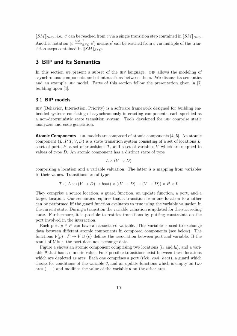
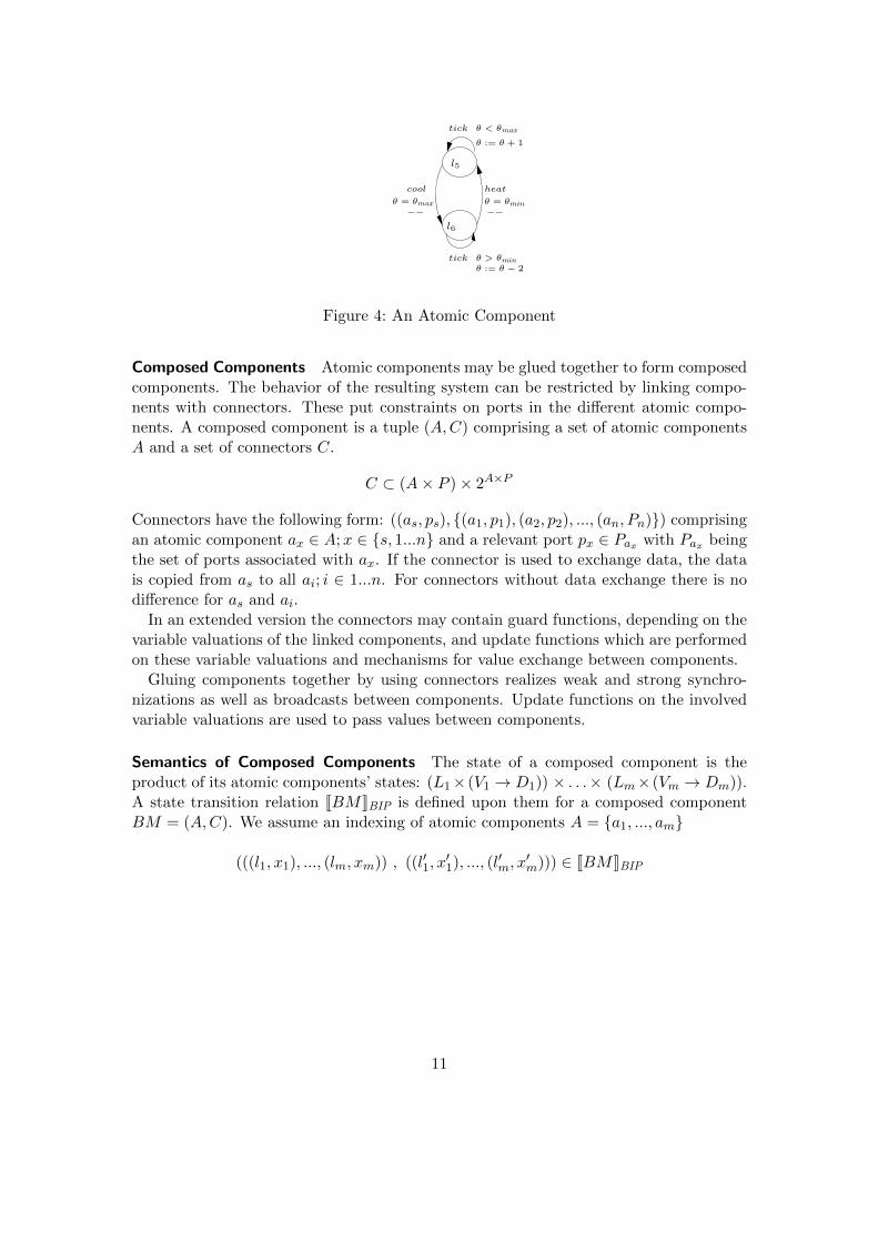
Figure 4 shows an atomic component comprising two locations (l5 and l6), and a vari-able θ that has a numeric value. Four possible transitions exist between these locationswhich are depicted as arcs. Each one comprises a port (tick, cool, heat), a guard whichchecks for conditions of the variable θ, and an update functions which is empty on twoarcs (−−) and modifies the value of the variable θ on the other arcs.

10

−−

tick

l6

heat

tick

l5

θ < θmax

θ := θ + 1

cool

θ > θminθ := θ − 2

θ = θmax θ = θmin−−

Figure 4: An Atomic Component

Composed Components Atomic components may be glued together to form composedcomponents. The behavior of the resulting system can be restricted by linking compo-nents with connectors. These put constraints on ports in the different atomic compo-nents. A composed component is a tuple (A,C) comprising a set of atomic componentsA and a set of connectors C.

C ⊂ (A× P )× 2A×P

Connectors have the following form: ((as, ps), (a1, p1), (a2, p2), ..., (an, Pn)) comprisingan atomic component ax ∈ A;x ∈ s, 1...n and a relevant port px ∈ Pax with Pax beingthe set of ports associated with ax. If the connector is used to exchange data, the datais copied from as to all ai; i ∈ 1...n. For connectors without data exchange there is nodifference for as and ai.

In an extended version the connectors may contain guard functions, depending on thevariable valuations of the linked components, and update functions which are performedon these variable valuations and mechanisms for value exchange between components.

Gluing components together by using connectors realizes weak and strong synchro-nizations as well as broadcasts between components. Update functions on the involvedvariable valuations are used to pass values between components.

Semantics of Composed Components The state of a composed component is theproduct of its atomic components’ states: (L1× (V1 → D1)) × . . .× (Lm× (Vm → Dm)).A state transition relation JBMKBIP is defined upon them for a composed componentBM = (A,C). We assume an indexing of atomic components A = a1, ..., am

(((l1, x1), ..., (lm, xm)) , ((l′1, x′1), ..., (l′m, x

′m))) ∈ JBMKBIP

11

iff

∃(cs, Cr) ∈ C : ∀i ∈ 1...m :

(∃j ∈ 1...m :

(∃p : (aj , p) = qs ∧ V(p) = vj)

∧ V(pi) = vi

∧ (li, gi, fi, pi, l′i) ∈ ai.T

∧ gi(xi)∧ x′i = fi(xi)[vi ← xj(vj)]

∧ (ai, pi) ∈ (cs ∪ Cr))∨(li = l′i

∧ ¬(∃p : (ai, p) ∈ (cs ∪ Cr))

∧ xi = x′i)

ai.T denotes the set of transitions associated with component ai

Reachable States of BIP models The set of reachable states for a bip model BM fora given initial state s0 is defined by a predicate RBM via the following inductive rules:

RBM (s0)

RBM (s) (s, s′) ∈ JBMKBIPRBM (s′)

The first rule says that the initial state is reachable. The second inference rule capturesthe transition behavior of bip using the transition relation.

3.2 An Example

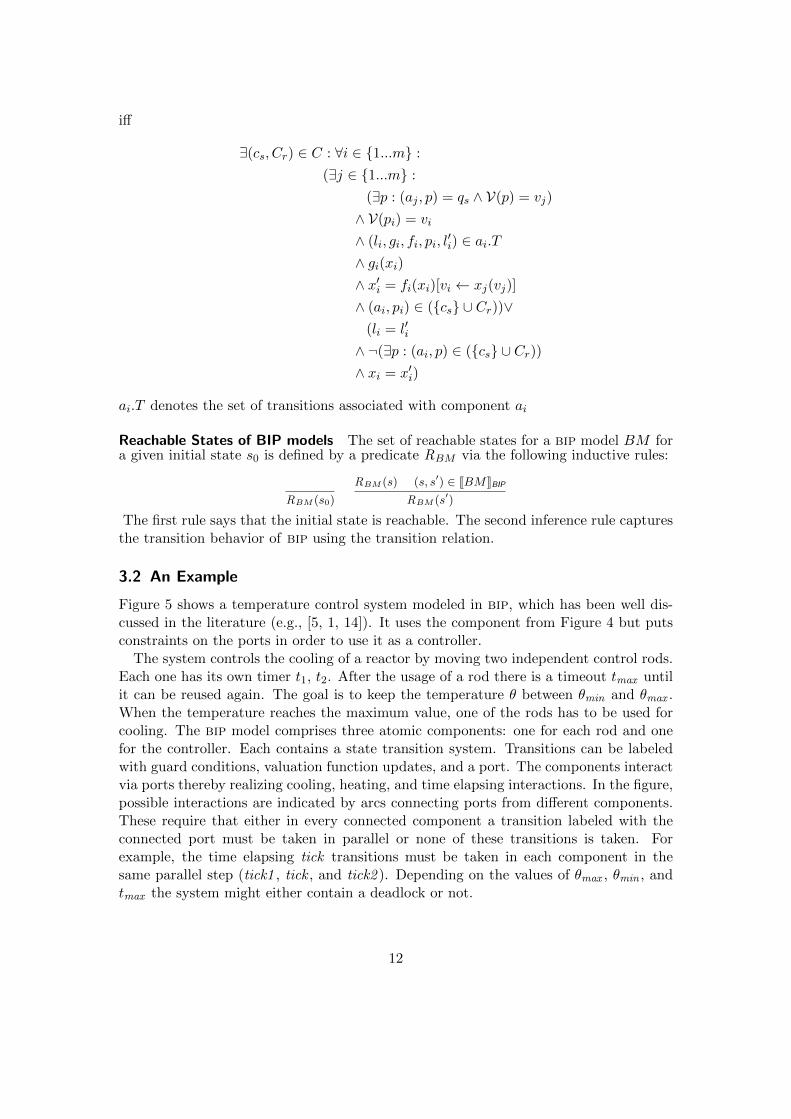
Figure 5 shows a temperature control system modeled in bip, which has been well dis-cussed in the literature (e.g., [5, 1, 14]). It uses the component from Figure 4 but putsconstraints on the ports in order to use it as a controller.

The system controls the cooling of a reactor by moving two independent control rods.Each one has its own timer t1, t2. After the usage of a rod there is a timeout tmax untilit can be reused again. The goal is to keep the temperature θ between θmin and θmax .When the temperature reaches the maximum value, one of the rods has to be used forcooling. The bip model comprises three atomic components: one for each rod and onefor the controller. Each contains a state transition system. Transitions can be labeledwith guard conditions, valuation function updates, and a port. The components interactvia ports thereby realizing cooling, heating, and time elapsing interactions. In the figure,possible interactions are indicated by arcs connecting ports from different components.These require that either in every connected component a transition labeled with theconnected port must be taken in parallel or none of these transitions is taken. Forexample, the time elapsing tick transitions must be taken in each component in thesame parallel step (tick1 , tick , and tick2 ). Depending on the values of θmax , θmin , andtmax the system might either contain a deadlock or not.

12

Rod2

tick

l6

heat

tick

l5

θ = θmin

θ < θmax

θ := θ + 1

cool

θ > θminθ := θ − 2

θ = θmax

t1 := t1 + 1

tick1

tick1

cool1t1 := 0

rest1

l1

l2

tick2

tick2

l3

l4

cool2 rest2t2 := 0

t2 := t2 + 1

tick tick2tick1

rest1 cool1 cool heat rest2 cool2

t1 ≥ tmax t2 ≥ tmax

Rod1 Controller

Figure 5: Temperature Control System

Let us introduce two invariants for the example model with θmax = 1000, θmin = 100,and tmax = 3600:

1. I1 ≡ (atl5 ∧ 100 ≤ θ ≤ 1000) ∨ (atl6 ∧ 100 ≤ θ ≤ 1000)This invariant states that the temperature will always be between 100 and 1000.

2. I2 ≡ (atl1 ∧ t1 = 0) ∨ (atl3 ∧ t2 = 0) ∨ (atl5 ∧ 101 ≤ θ ≤ 1000)∨(atl6 ∧ (θ = 1000 ∨ 100 ≤ θ ≤ 998))This invariant states that the timer in one of the rods is zero or we are in theheating phase and the temperature is already above 100 or we are in the coolingphase and the temperature is 1000 or between 100 and 998.

ati is a predicate denoting the fact that we are at location i in a component. The firstinvariant is restricted to a single component, the second one combines facts about severalcomponents.

4 Transformation from SFCs to BIP

This sections describes the transformation rules from the SFC language to bip.For a given SFC S = (X,A, S, S0, T,@,≺, h), the transformed bip model can be

represented by a composed component B = (A, C), with A ⊂ L×P×T×V ×D being the

set of atomic components and C ⊂ (A×P )×2A×P the set of connectors. In the followingsections, we first describes the atomic components including their formal definition (4.1),and afterward the transformations steps and connections of atomic components (4.2).

SFC evaluation phases As introduced in Section 2.2, execution of an SFC is done inSFC cycles, which consists of three phases:

1. execution of active actions,

13

2. evaluation of transitions and identification of active steps,

3. identification of active actions for the next cycle.

In the generated bip model, an SFCManager component is introduced to enforce syn-chronization of the phases. This is done with the wTick (work tick), tT ick (transitiontick) and fT ick (finish tick) signals.

4.1 Atomic Components

Several transformation templates can be identified for the transformation of SFC ele-ments into bip elements.

Actions Each SFC action a ∈ A will be represented by a bip component a ∈ A. Eachaction has two ports for synchronization with the bip representation of the SFC program.The work port starts the action. Then it reads all input data, processes the data andwrites the output value. At last is enables the done port to signal its ACB (see nextparagraph) that it has finished processing.

To access global variables, the action has a readx and/or a writex for each variablex is accesses. They are connected to the read and write ports of the global variableatomics.

Action Control Blocks For an action component a ∈ A transformed from an SFC ac-tion a ∈ A, a special atomic component called Action Control Block (ACB) is equipped,which is responsible for collect and evaluate qualifiers from action activations to decideif the action will be executed for the next SFC cycle. We use ba to denote the ACBcomponent created for a and B for the set of ACB components for all actions.

Transformation 1 (Action Control Block)

CreateACB(a) : A→ L× P × T × L× V ×DCreateACB(a) = (LACB, PACB, TACB, L0ACB , VACB, DACB)

14

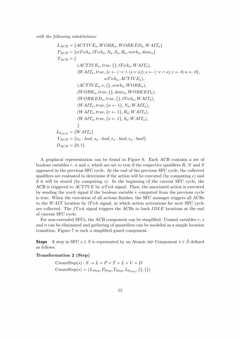
with the following substitutions:

LACB = ACTIV Ea,WORKa,WORKEDa,WAITaPACB = wTicka, tT icka, Na, Sa, Ra, worka, doneaTACB =

(ACTIV Ea, true, , tT icka,WAITa),

(WAITa, true, e← (¬r ∧ (s ∨ n)); s← (¬r ∧ s); r ← 0;n← 0,wT icka, ACTIV Ea),

(ACTIV Ea, e, , worka,WORKa),

(WORKa, true, , donea,WORKEDa),

(WORKEDa, true, , tT icka,WAITa),

(WAITa, true, n← 1, Na;WAITa),

(WAITa, true, r ← 1, Ra;WAITa),

(WAITa, true, s← 1, Sa;WAITa),

L0ACB = WAITaVACB = na : bool, sa : bool, ra : bool, ea : boolDACB = 0, 1

A graphical representation can be found in Figure 6. Each ACB contains a set ofboolean variables r, n and s, which are set to true if the respective qualifiers R, N and Sappeared in the previous SFC cycle. At the end of the previous SFC cycle, the collectedqualifiers are evaluated to determine if the action will be executed (by computing e) andif it will be stored (by computing s). In the beginning of the current SFC cycle, theACB is triggered to ACTIV E by wTick signal. Then, the associated action is executedby sending the work signal if the boolean variable e computed from the previous cycleis true. When the execution of all actions finishes, the SFC manager triggers all ACBsto the WAIT location by tT ick signal, in which action activations for next SFC cycleare collected. The fT ick signal triggers the ACBs to back IDLE locations at the endof current SFC cycle.

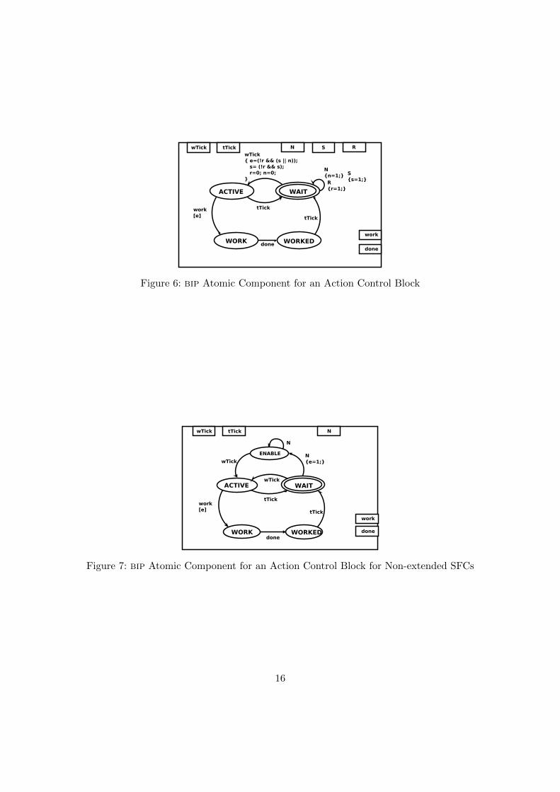
For non-extended SFCs, the ACB component can be simplified. Unused variables r, sand n can be eliminated and gathering of quantifiers can be modeled as a simple locationtransition. Figure 7 is such a simplified guard component.

Steps A step in SFC s ∈ S is represented by an Atomic bip Component s ∈ S definedas follows.

Transformation 2 (Step)

CreateStep(s) : S → L× P × T × L× V ×DCreateStep(s) = (LStep, PStep, TStep, L0Step , , )

15

ACTIVE WAIT

WORK WORKED

wTick e=(!r && (s || n)); s= (!r && s); r=0; n=0;

Nn=1;

tTick

tTick

done

work[e]

wTick tTick S

work

done

RN

Ss=1;

Rr=1;

Figure 6: bip Atomic Component for an Action Control Block

ACTIVE WAIT

WORK WORKED

wTick

Ne=1;

tTick

tTick

done

work[e]

wTick tTick N

work

done

ENABLE

N

wTick

Figure 7: bip Atomic Component for an Action Control Block for Non-extended SFCs

16

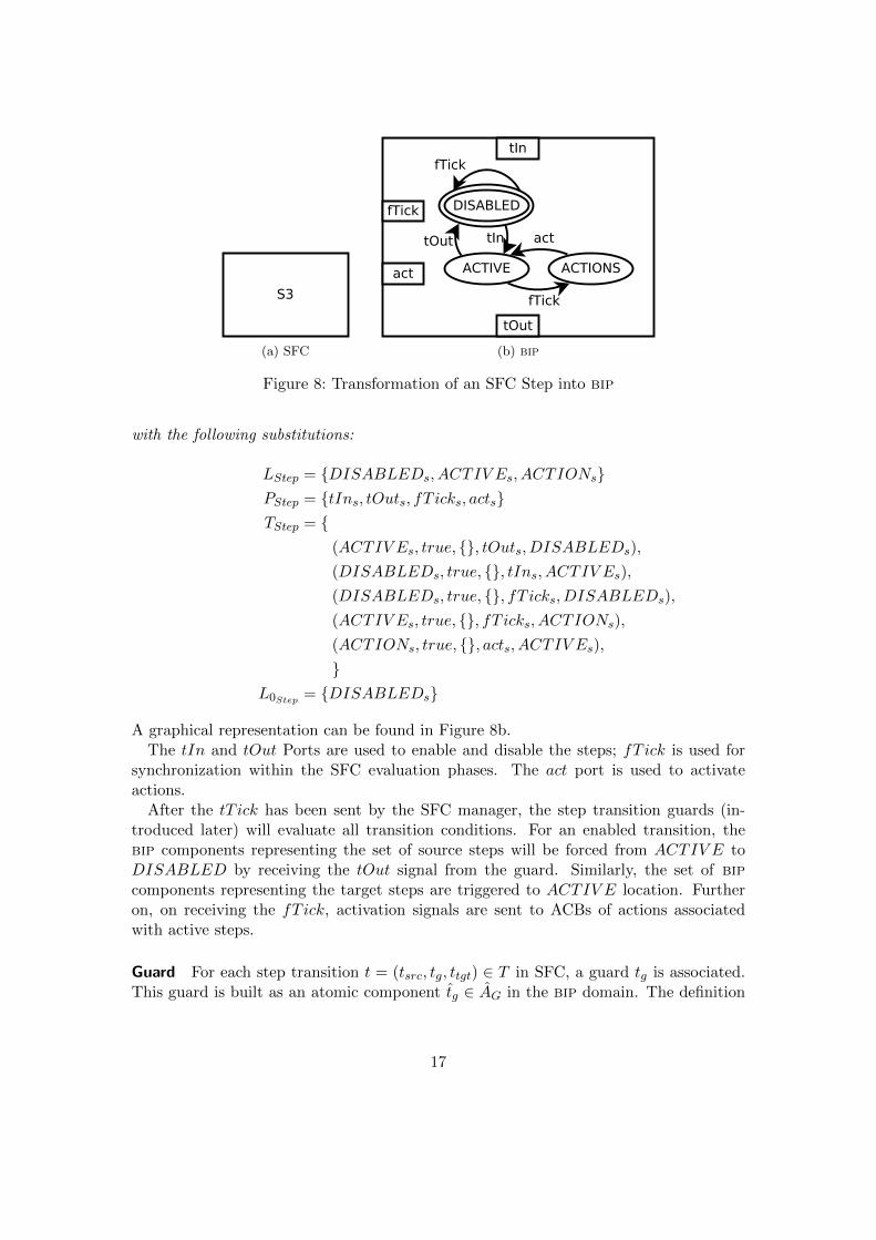
S3

(a) SFC

tIn

act

tOut

DISABLED

ACTIONS

tIntOut

fTick

fTick

act

ACTIVE

fTick

(b) bip

Figure 8: Transformation of an SFC Step into bip

with the following substitutions:

LStep = DISABLEDs, ACTIV Es, ACTIONsPStep = tIns, tOuts, fT icks, actsTStep =

(ACTIV Es, true, , tOuts, DISABLEDs),

(DISABLEDs, true, , tIns, ACTIV Es),

(DISABLEDs, true, , fT icks, DISABLEDs),

(ACTIV Es, true, , fT icks, ACTIONs),

(ACTIONs, true, , acts, ACTIV Es),

L0Step = DISABLEDs

A graphical representation can be found in Figure 8b.The tIn and tOut Ports are used to enable and disable the steps; fT ick is used for

synchronization within the SFC evaluation phases. The act port is used to activateactions.

After the tT ick has been sent by the SFC manager, the step transition guards (in-troduced later) will evaluate all transition conditions. For an enabled transition, thebip components representing the set of source steps will be forced from ACTIV E toDISABLED by receiving the tOut signal from the guard. Similarly, the set of bipcomponents representing the target steps are triggered to ACTIV E location. Furtheron, on receiving the fT ick, activation signals are sent to ACBs of actions associatedwith active steps.

Guard For each step transition t = (tsrc, tg, ttgt) ∈ T in SFC, a guard tg is associated.This guard is built as an atomic component tg ∈ AG in the bip domain. The definition

17

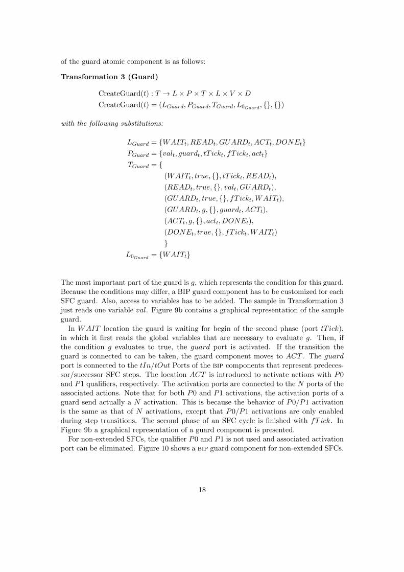
of the guard atomic component is as follows:

Transformation 3 (Guard)

CreateGuard(t) : T → L× P × T × L× V ×DCreateGuard(t) = (LGuard, PGuard, TGuard, L0Guard , , )

with the following substitutions:

LGuard = WAITt, READt, GUARDt, ACTt, DONEtPGuard = valt, guardt, tT ickt, fT ickt, acttTGuard =

(WAITt, true, , tT ickt, READt),

(READt, true, , valt, GUARDt),

(GUARDt, true, , fT ickt,WAITt),

(GUARDt, g, , guardt, ACTt),(ACTt, g, , actt, DONEt),

(DONEt, true, , fT ickt,WAITt)

L0Guard = WAITt

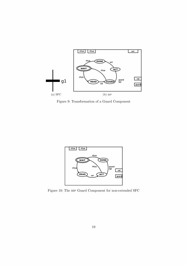
The most important part of the guard is g, which represents the condition for this guard.Because the conditions may differ, a BIP guard component has to be customized for eachSFC guard. Also, access to variables has to be added. The sample in Transformation 3just reads one variable val. Figure 9b contains a graphical representation of the sampleguard.

In WAIT location the guard is waiting for begin of the second phase (port tT ick),in which it first reads the global variables that are necessary to evaluate g. Then, ifthe condition g evaluates to true, the guard port is activated. If the transition theguard is connected to can be taken, the guard component moves to ACT . The guardport is connected to the tIn/tOut Ports of the bip components that represent predeces-sor/successor SFC steps. The location ACT is introduced to activate actions with P0and P1 qualifiers, respectively. The activation ports are connected to the N ports of theassociated actions. Note that for both P0 and P1 activations, the activation ports of aguard send actually a N activation. This is because the behavior of P0/P1 activationis the same as that of N activations, except that P0/P1 activations are only enabledduring step transitions. The second phase of an SFC cycle is finished with fT ick. InFigure 9b a graphical representation of a guard component is presented.

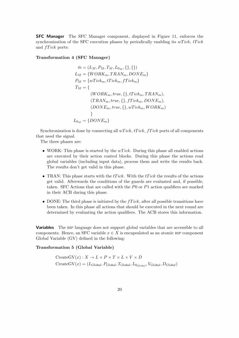
For non-extended SFCs, the qualifier P0 and P1 is not used and associated activationport can be eliminated. Figure 10 shows a bip guard component for non-extended SFCs.

18

g1

(a) SFC

WAIT

READ GUARD

fTick

val

tTick

tTick fTick

ACT

DONE

fTick

act

guard[g]

act

val

guard

(b) bip

Figure 9: Transformation of a Guard Component

WAIT

READ ACT

fTick

val

tTick

tTick fTick

DONE

fTick guard[g]

val

guard

Figure 10: The bip Guard Component for non-extended SFC

19

SFC Manager The SFC Manager component, displayed in Figure 11, enforces thesynchronization of the SFC execution phases by periodically enabling its wTick, tT ickand fT ick ports:

Transformation 4 (SFC Manager)

m = (LM , PM , TM , L0M , , )LM = WORKm, TRANm, DONEmPM = wTickm, tT ickm, fT ickmTM =

(WORKm, true, , tT ickm, TRANm),

(TRANm, true, , fT ickm, DONEm),

(DONEm, true, , wT ickm,WORKm)

L0M = DONEm

Synchronization is done by connecting all wTick, tT ick, fT ick ports of all componentsthat need the signal.

The three phases are:

• WORK: This phase is started by the wTick. During this phase all enabled actionsare executed by their action control blocks. During this phase the actions readglobal variables (including input data), process them and write the results back.The results don’t get valid in this phase.

• TRAN: This phase starts with the tT ick. With the tT ick the results of the actionsget valid. Afterwards the conditions of the guards are evaluated and, if possible,taken. SFC Actions that are called with the P0 or P1 action qualifiers are markedin their ACB during this phase.

• DONE: The third phase is initiated by the fT ick, after all possible transitions havebeen taken. In this phase all actions that should be executed in the next round aredetermined by evaluating the action qualifiers. The ACB stores this information.

Variables The bip language does not support global variables that are accessible to allcomponents. Hence, an SFC variable x ∈ X is encapsulated as an atomic bip componentGlobal Variable (GV) defined in the following:

Transformation 5 (Global Variable)

CreateGV(x) : X → L× P × T × L× V ×DCreateGV(x) = (LGlobal, PGlobal, TGlobal, L0Global , VGlobal, DGlobal)

20

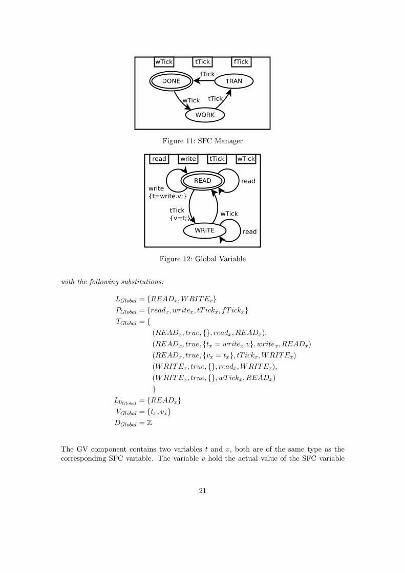
Figure 11: SFC Manager

read write

WAITwritet=write.v;

readREAD

WRITE

tTickv=t;

wTick

read

wTicktTick

Figure 12: Global Variable

with the following substitutions:

LGlobal = READx,WRITExPGlobal = readx, writex, tT ickx, fT ickxTGlobal =

(READx, true, , readx, READx),

(READx, true, tx = writex.v, writex, READx)

(READx, true, vx = tx, tT ickx,WRITEx)

(WRITEx, true, , readx,WRITEx),

(WRITEx, true, , wT ickx, READx)

L0Global = READxVGlobal = tx, vxDGlobal = Z

The GV component contains two variables t and v, both are of the same type as thecorresponding SFC variable. The variable v hold the actual value of the SFC variable

21

tOut

ACTIVE

DISABLED

tOut

ACTIVE

wTickwTick

Figure 13: SFC Starter

whereas t is a temporary buffer. Initially, the GV component is in READ location, inwhich reading of the variable value is allowed and writing of the variable is bufferedin t. The buffer value is written to v on receiving the tT ick signal, that is, when allactions has been performed. This guarantees that all actions read the consistent valueof v. On the other hand, the buffered value is written immediately with the tT ick, sothat the guard components can read the up-to-date value of variables and evaluate thetransition conditions correctly. The wTick brings the GV back to WRITE location.Figure 12 is the graphical representation of the GV component, in which write.v is thevalue exchanged via the write port.

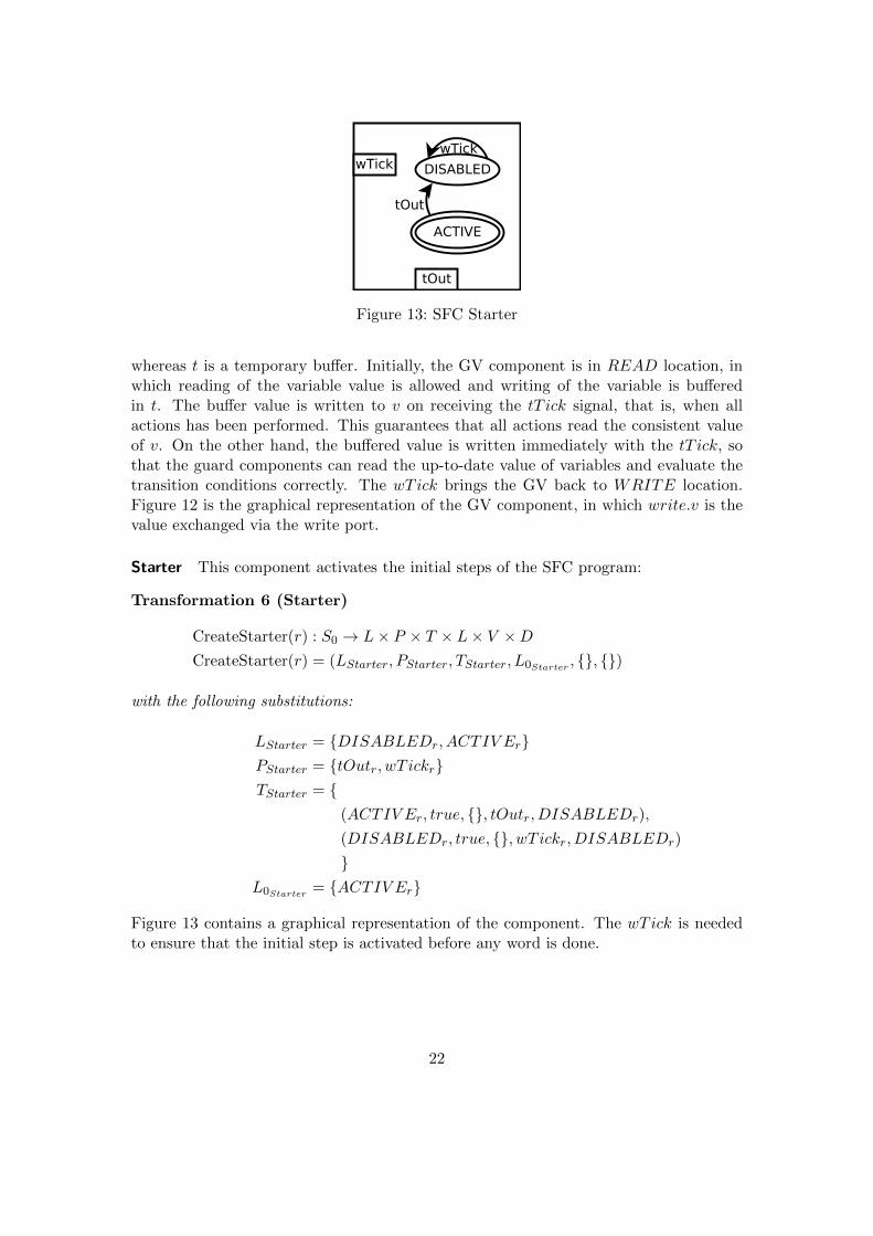
Starter This component activates the initial steps of the SFC program:

Transformation 6 (Starter)

CreateStarter(r) : S0 → L× P × T × L× V ×DCreateStarter(r) = (LStarter, PStarter, TStarter, L0Starter , , )

with the following substitutions:

LStarter = DISABLEDr, ACTIV ErPStarter = tOutr, wT ickrTStarter =

(ACTIV Er, true, , tOutr, DISABLEDr),

(DISABLEDr, true, , wT ickr, DISABLEDr)

L0Starter = ACTIV Er

Figure 13 contains a graphical representation of the component. The wTick is neededto ensure that the initial step is activated before any word is done.

22

S1

(a) SFC

Starter

tOut

S1

tIn

(b) bip

Figure 14: Initial Step

F2X

Xw

read

write

Xr

Figure 15: Use of Global Variable X in F2

4.2 Transformation Steps

The following describes the steps necessary to convert an SFC program to a compoundbip component. All created instances of atomics are added to A.

For each global variable x ∈ X we create an instance of the bip Global Variable atomiccomponent x:

AX := x := CreateGV(x)|x ∈ X

For each Action a ∈ A create an instance a of it in bip.

AA := a := CreateAction(a)|a ∈ A

For each Action a ∈ A create an instance of ACB component ba in bip and connect thework and done ports correspondingly (see Figure 16b).

AB :=ba := CreateACB(a)|a ∈ A

CA :=

((ba, work

), (a, work)

)|a ∈ AA

∪((

ba, done), (a, done)

)|a ∈ AA

23

N F2

S F3S3

(a) SFC

F2

B2

done

work done

work

S3

F3

B3

done

work done

work

act

N S R N S R

(b) bip

Figure 16: Action

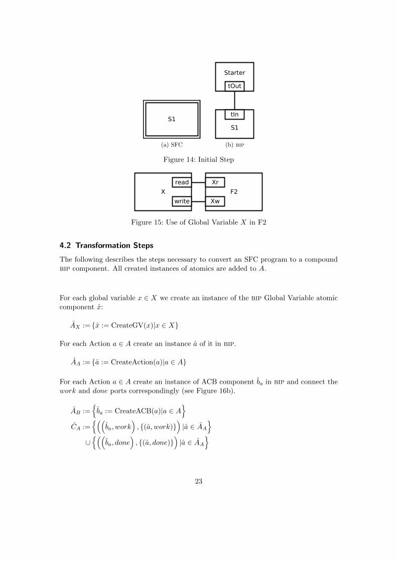
For each SFC Step s ∈ S instantiate the bip Step component s.

AS := s := CreateStep(s)|s ∈ S

For each initial step s ∈ S0 create a bip Starter instance rs and create a connector to s(Figure 14).

AS0 := rs := CreateStarter(s)|s ∈ S0CS0 :=((ts, tOut), (s, tIn))|ts ∈ AS0

For each SFC transition (tsrc, g, tdst) = t ∈ T create a guard component gt in bipand connect it to tOut of tsrc and tIn of ttgt. If the reading of variables is neededfor evaluating the condition, necessary read ports, locations and transitions are createdaccording to Figure 9.

AG := gt := CreateStarter(t)|t ∈ T

CT :=⋃

(tsrc,tg ,ttgt)=t∈T

(gt, guard) ,

⋃s∈tsrc

(s, tOut) ∪⋃

s∈ttgt

(s, tIn)

Connect all actions and guards to global variables if necessary (see Figure 15).

CX :=⋃

(x,a)∈AX×AA

((x, read) , (a, xr)) , ((a, xw) , (x, write))

∪⋃

(x,g)∈AX×AG

((x, read) , (a, xr))

24

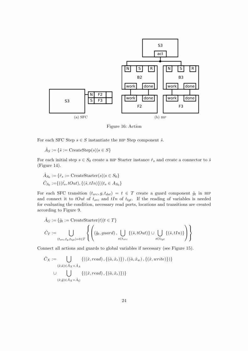
S3

S4

(a) SFC

GuardS3

gtOut

S4

tIn

(b) bip

Figure 17: Transition

For each step s ∈ S create a connector to the ACB b of all actions it activates. Use theport of the ACB according to the action qualifier. For the P0/P1 qualifier connect theN port of the ACB to the guards act port.

CB :=⋃s∈S

(s, act) ,

⋃(a,q)∈s.Ωq∈N,S,R

(ba, q

)

∪⋃

(tsrc,tg ,ttgt)=t∈T

(gt, act) ,

⋃(a,P0)∈s.Ω

s∈tsrc

(ba, N

)∪

⋃(a,P1)∈s.Ω

s∈ttgt

(ba, N

)

Create an instance of the SFC manager component m and connect the wTick, tT ickand fT ick ports to all components that expect these signal.

CM :=((m, wT ick), (a, wT ick)|a ∈ AB ∪ AX ∪ AS0)∪((m, tT ick), (a, tT ick)|a ∈ AB ∪ AG ∪ AX)∪((m, fT ick), (a, fT ick)|a ∈ AS ∪ AG)

Putting everything together

A :=AX ∪ AA ∪ AB ∪ AS ∪ AS0 ∪ AG ∪ mC :=CX ∪ CA ∪ CS0 ∪ CT ∪ CB ∪ CM

B :=(A, C)

In the following some samples for the transformation of transition are provided.

25

S3

S4 S5

(a) SFC

G3a S3

g tOut

S4

tIn

G3b

g

S5

tIn

(b) bip

Figure 18: Divergence

S4

S2 S3

(a) SFC

S3

G3

S2

g

tOut

S4

tIn

tOut

G2

g

(b) bip

Figure 19: Convergence

26

S2

S3 S4

(a) SFC

S2

tOut

S3

tIn

Guard

g

S4

tIn

(b) bip

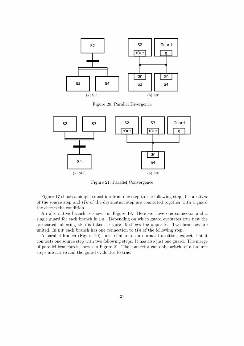
Figure 20: Parallel Divergence

S4

S2 S3

(a) SFC

S3 GuardS2

gtOut

S4

tIn

tOut

(b) bip

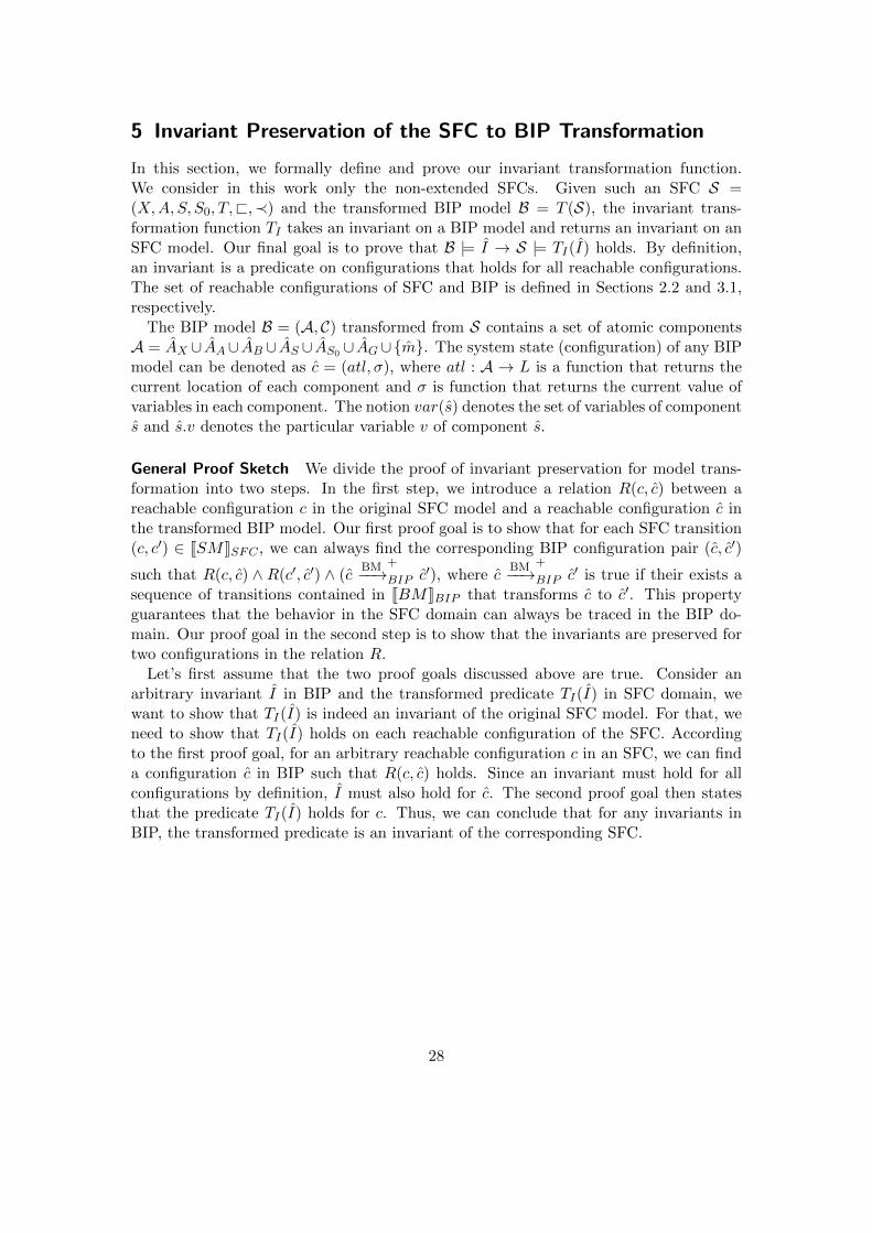
Figure 21: Parallel Convergence

Figure 17 shows a simple transition from one step to the following step. In bip tOutof the source step and tIn of the destination step are connected together with a guardthe checks the condition.

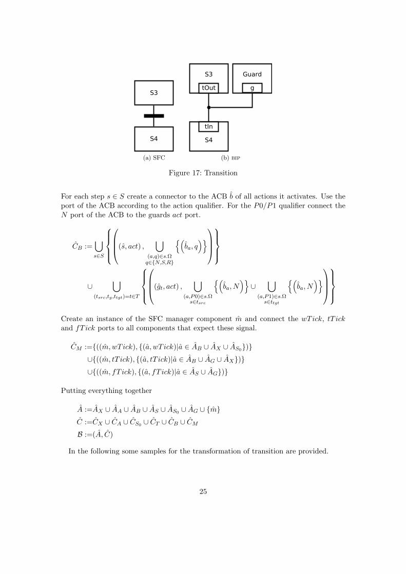
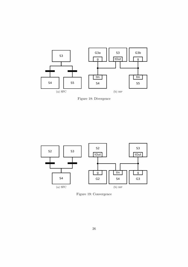
An alternative branch is shown in Figure 18. Here we have one connector and asingle guard for each branch in bip. Depending on which guard evaluates true first theassociated following step is taken. Figure 19 shows the opposite. Two branches areunited. In bip each branch has one connection to tIn of the following step.

A parallel branch (Figure 20) looks similar to an normal transition, expect that itconnects one source step with two following steps. It has also just one guard. The mergeof parallel branches is shown in Figure 21. The connector can only switch, of all sourcesteps are active and the guard evaluates to true.

27

5 Invariant Preservation of the SFC to BIP Transformation

In this section, we formally define and prove our invariant transformation function.We consider in this work only the non-extended SFCs. Given such an SFC S =(X,A, S, S0, T,@,≺) and the transformed BIP model B = T (S), the invariant trans-formation function TI takes an invariant on a BIP model and returns an invariant on anSFC model. Our final goal is to prove that B |= I → S |= TI(I) holds. By definition,an invariant is a predicate on configurations that holds for all reachable configurations.The set of reachable configurations of SFC and BIP is defined in Sections 2.2 and 3.1,respectively.

The BIP model B = (A, C) transformed from S contains a set of atomic componentsA = AX ∪ AA∪ AB ∪ AS ∪ AS0 ∪ AG∪m. The system state (configuration) of any BIPmodel can be denoted as c = (atl, σ), where atl : A → L is a function that returns thecurrent location of each component and σ is function that returns the current value ofvariables in each component. The notion var(s) denotes the set of variables of components and s.v denotes the particular variable v of component s.

General Proof Sketch We divide the proof of invariant preservation for model trans-formation into two steps. In the first step, we introduce a relation R(c, c) between areachable configuration c in the original SFC model and a reachable configuration c inthe transformed BIP model. Our first proof goal is to show that for each SFC transition(c, c′) ∈ JSMKSFC , we can always find the corresponding BIP configuration pair (c, c′)

such that R(c, c) ∧ R(c′, c′) ∧ (cBM−−→

+

BIP c′), where cBM−−→

+

BIP c′ is true if their exists asequence of transitions contained in JBMKBIP that transforms c to c′. This propertyguarantees that the behavior in the SFC domain can always be traced in the BIP do-main. Our proof goal in the second step is to show that the invariants are preserved fortwo configurations in the relation R.

Let’s first assume that the two proof goals discussed above are true. Consider anarbitrary invariant I in BIP and the transformed predicate TI(I) in SFC domain, wewant to show that TI(I) is indeed an invariant of the original SFC model. For that, weneed to show that TI(I) holds on each reachable configuration of the SFC. Accordingto the first proof goal, for an arbitrary reachable configuration c in an SFC, we can finda configuration c in BIP such that R(c, c) holds. Since an invariant must hold for allconfigurations by definition, I must also hold for c. The second proof goal then statesthat the predicate TI(I) holds for c. Thus, we can conclude that for any invariants inBIP, the transformed predicate is an invariant of the corresponding SFC.

28

The relation R can be formally defined as follows:

∀c = (f, activeS, activeA), ∀c = (atl, σ), R(c, c) holds iff

rule1(c, c) ∧ rule2(c, c) ∧ rule3(c, c), where

rule1(c, c) = ∀ s ∈ S, s ∈ AS . s ∈ activeS ≡ ¬(atl(s) = DISABLE)

rule2(c, c) = ∀ a ∈ A, a ∈ AA, ba ∈ AB . a ∈ activeA ≡ (σ(ba.e) = 1)

rule3(c, c) = ∀ x ∈ X, x ∈ AX . f(x) = σ(x.v)

The first step of the proof is to shown that both G1a and G1b holds:

G1a : R(c0, c0)

G1b : ∀c, c′, c . c SM−−→SFC c′ ∧R(c, c)

→ ∃c′ . c BM−−→+

BIP c′ ∧R(c′, c′) ∧BM = T (SM)

The second step of our proof is to show that for all configuration pairs in the relation,the invariant is preserved. Formally, the second proof goal G2 is:

G2 = ∀c, c . R(c, c) → (∀I . c |= I → c |= TI(I))

where I is a invariant in BIP model and TI is the invariant transformation function thatmaps I to an invariant in SFC domain. The notion c |= I means c satisfies I.

Proof of G1a The proof that G1a = R(c0, c0) holds can be done based on the modeltransformation rules:

• for each initially active step, a starter component is added in the BIP model, whichtriggers the step component to the ACTIV E location (rule1 fulfilled);

• no action should be active in c0 and the initial value of variable e in the ACBblocks are set to false (rule2 fulfilled);

• the value of variable v of GV components are initialized according to the SFCvariables (rule3 fulfilled).

Based on the above transformation rules, it can be trivially shown that the R(c0, c0)holds.

Proof of G1b For the subgoal G1b, we make a case distinction on three possible typesof transitions of the SFC.

1. In an executeAction transition, some action a is executed which updates the valueof SFC variables. An action can be executed only if it is active, hence, a ∈activeA. In the corresponding BIP model, the SFC manager enforces that all

29

action execution is performed between the fT ick of the previous cycle and thetT ick of the current cycle. Let a be the action component and ba be the ACBcomponent created for a. Since the relation R(c, c) holds, the e variable in bais true according to rule2. From the structure of ACB component (Figure 7),we can see that ba can be on the ENABLE, IDLE or ACTIV E location. Inall cases, the transition from location ACTIV E to WORK will be taken afternext wTick signal. This transition triggers the execution of action component a,which performs the same set of operations as specified in a, because the modeltransformation just copies those operations. The transition also set the value ofba.e to false. Execution sequence of the actions in the BIP model is guaranteedto be the same as in original SFC model, since transition from location ACTIV Eto WORK in each ACB component is prioritized according to the order @. Letc′ be the BIP configuration in which the action a is just done (ba in WORKEDlocation). It can be easily seen that rule2 in the definition of relation R holdsfor (c′, c′). On the other hand, since tT ick interaction has the lowest priority, notT ick is issued during the transition from c to c′. So, no step component goes tolocation DISABLE, which means rule1 holds for (c′, c′). In addition, the relationR(c, c) says that the current values of variable v in GV components are the sameas that of SFC variables X. Hence, the input of operations in a is the same as thatof a. Since component a doesn’t contain any internal variables, the output valueswill be the same, thus rule3 holds for R(c′, c′). We can conclude that we reach anconfiguration c′ such that R(c′, c′) holds.

2. In a stepTransition, the set of active steps is updated by taking some enabledtransition t and the rest of the configuration is not affected. According to the op-erational semantics of SFCs, step transitions are performed after execution of allactive actions identified from the previous cycle. In the transformed BIP model,we achieve this point after the tT ick signal. At this moment, all ACB compo-nents are in WAIT location and all guard components are ready to read valuesfrom GV components. Let tg be the guard component created for t. Accord-ing to the relation R(c, c), the variable values of GV components are the sameas SFC variables X. This guarantees that, if t can be taken in the originalSFC model, the condition g in the tg component must evaluate to true. Dur-ing model transformation, the transitions from location ACT to DONE in allguard components are assigned to higher priority than fT ick, hence, the interac-tion ((tg, guard), (s1, tOut), ..., (sn, tOut), (s1, tOut), ..., (sm, tOut)) will be takenbefore next fT ick signal, where s1, ...sn are BIP atomics created for steps s ∈ tsrcand s1, ..., sm are the corresponding components for steps s ∈ ttgt. This inter-action triggers all source steps of transition t to DISABLE location and triggersall target steps of t to ACTIV E location. It can be easily shown that the rule1

of relation R is fulfilled after this interaction. On the other hand, in both SFCand BIP model, the set of active actions and the values of variables do not change.Thus we reach a configuration c′ such that R(c′, c′) holds.

30

3. The third type of SFC configuration transition is the computation of active actions,which is the last phase in an SFC execution cycle. In the transformed BIP model,we reach this point after an fT ick interaction. The relation R(c, c) says that foreach active step in the SFC, the corresponding step component in BIP must notin DISABLE location. Hence, before the next wTick, all active steps compo-nents will activate the associated actions (Figure 8), since wTick interaction hasthe lowest priority. According to the model transformation rules, for each actioncontained in the set Ω, a connector is constructed that connects the activation portof the step component with the ACB component. Thus, the set of active actionswill be the same in both SFC and BIP models, given the set of active steps are thesame. This guaranteed that rule2 holds. Since the rest part of the configurationdoesn’t change in both models, we reach a configuration c′ such that R(c′, c′) holds.

As shown above, for all types of configuration transitions in SFC, the proof goal G1bholds. Note that we made the implicit assumption in our proof that we either use thesame datatypes for both SFC and BIP model or no overflows and underflows of valueranges occur.

Before we present a proof of G2, a formalism for describing the invariants in SFCsand BIP models is needed, which is presented in the following paragraphs.

Invariants on SFC The syntax of an SFC invariant can be expressed as follows:

I ::= i ∧ ii ::= i′

i′ ::= i′ ∨ i′

i′ ::= i′′

i′′ ::= ¬i′′

i′′ ::= C | AS| AAC ::= cond(X)

AS ::= s ∈ activeSAA ::= a ∈ activeA

Where cond(X) is a predicate on the set of SFC variables X. For an SFC, we can stati-cally analyze the model and find the activation relation between steps and actions, whichcan help us to express the invariants in SFC models. Let SN (a) = s ∈ S | a ∈ s.Ωdenote the set of steps associated with an action a. A structural invariant that holds forall non-extended SFCs is:

∨s∈SN (a)

s ∈ activeS

∧ a ∈ activeA ∨

∧s∈SN (a)

¬(s ∈ activeS)

∧ ¬(a ∈ activeA)

31

This invariant says if at least one step that can invoke the action a is in active state,the action a is also in active state, otherwise a is not active.

Invariants on BIP Models An invariant in a BIP model can be expressed using thefollowing syntax:

I ::= i

i ::= i ∧ ii ::= i′

i′ ::= i′ ∨ i′

i′ ::= i′′

i′′ ::= ¬i′′

i′′ ::= C | L | C ∧ LC ::= cond(var(s))

L ::= atl(s) = l

where atl(s) = l is true if the component s is at location l, and cond(var(s)) is apredicate on the variables of s. The structure of this invariant language reflects theinvariant generated by D-Finder [5]. Some examples are given in Section 3.2.

Invariant Transformation From the previous definition, we see that any BIP invariantcan be written as logical expressions of two basic sets of elements: predicates on variablesof individual component and predicates on locations of individual components. Weintroduce an invariant transformation function TI , which takes an BIP invariant I andreturns the corresponding invariant in the SFC domain. It is defined inductively:

TI(I1 ∧ I2) = TI(I1) ∧ TI(I2)

TI(I1 ∨ I2) = TI(I1) ∨ TI(I2)

...

As it can be seen, the function TI keeps the structure of BIP invariants and maps eachelementary BIP predicate to a corresponding predicate in the SFC domain. Given aBIP model B = T (S) transformed from an SFC model S, the mapping of elementarypredicates on B to predicates on S is described using following rules. The notion s.Ldenotes the set of all locations of BIP atomic s.

1. For a predicate on variables p = cond(var(s)) we distinguish the following cases:

• if s is a GV component created for SFC variable x, s has only two variablesv and t by definition. Since the relationship between v and t is a simpleassignment, the condition can be written in the form condt(t) ∧ condv(v).Then, the corresponding predicate in SFC domain is TI(p) = condv(x), i.e.we ignore the condition on t and apply the condition on v to SFC variable x;

32

• if s is a ACB component, it contains a boolean variable e. The predicate pis a boolean expression on these variables. Let a be the corresponding SFCaction that s is created for, the transformation of p is done by keeping thestructure of expression and doing the replacement: TI(e) = a ∈ activeA;

• if s is an other component, TI(p) = true. Actually, this rule is not used,since only GV and ACB component contain variables according to the modeltransformation rules.

2. For predicates on locations we distinguish the following cases:

• if s is a step component, TI(atl(s) = DISABLE) = ¬(s ∈ activeS) andTI(atl(s) = l) = s ∈ activeS,∀ l ∈ s.L\DISABLE, where s is the step inSFC that s is transformed from;

• if s is a ACB component created for SFC action a, TI(atl(s) = ENABLE) =∨s∈SN (a)

s ∈ activeS and TI(atl(s) = l) = false, ∀l ∈ s.L\ENABLE;

• if s is other component, TI(p) = false.

In the invariant transformation procedure, some unused predicates on locations areeliminated by setting them to false in the transformed SFC invariant. This is safe becausethe BIP component invariants have a disjunction form as mentioned before.

Example. For an ACB component s (Figure 7), an obvious invariant can be found as:I = ¬(atl(s) = ENABLE)∨ (atl(s) = ENABLE ∧ e). By applying the transformationrules, we can obtain I = (¬

∨s∈SN (a)

s ∈ activeS) ∨ ((∨

s∈SN (a)

s ∈ activeS) ∧ a ∈ activeA),

which is an invariant contained in the example SFC structural invariant we found before.Another set of invariants that can be identified in BIP models are interaction in-

variants. Let’s consider a BIP model transformed from a simple SFC shown in Figure17. The transformed BIP model consists of (besides other necessary components) twostep atomics and one guard atomic. A connector (S3, tOut), (S4, tIn), (Guard, g) isbuilt by the transformation. The interaction described by the above connector is en-abled if atl(S3) = ACTIV E ∧ atl(S4) = DISABLE ∧ atl(Guard) = ACT ∧ Guard.ghold. An obvious interaction invariant that can be observed is that one of S3 and S4must be in DISABLE location, i.e. atl(S3) = DISABLE ∨ atl(S4) = DISABLEmust hold. By applying the transformation rules, the predicate in SFC domain is¬S3 ∈ activeS ∨ ¬S4 ∈ activeS, which obviously holds by the semantics of SFC.

Proof of G2 The proof of second goal comes strait forwardly from the definitionsof R and TI . Consider a configuration c of an SFC model and a configuration c ofthe transformed BIP model, we now show that if R(c, c) holds, then for an arbitraryinvariant I |= c in the BIP domain, the transformed predicate I = TI(I) holds for c inthe SFC domain. Since I and I have the same structure, it is sufficient to show that allthe elementary predicates in I evaluates to the same value as the transformed predicatesin I. We make a case distinction on the two types of predicates. The first type are

33

predicates on variables of some component s. We can see from the model transformationrules only the GV and ACB component contains internal variables. The rule2 and rule3

in the definition of R guarantees that the predicates before and after transformation TIevaluate to the same result. The second type are predicates on locations. As stated inthe definition of TI , only the predicates on step components and ACB components arekept. For the case of step components, the rule1 guarantees the correctness. For thecase of ACB components, the correctness comes from the structure of the ACB: whenwe move to the ENABLE location, at least one step component has interacted with theACB via the activation port, which means at least one step component must be activein the first place.

6 Transformation of SFC Safety Requirements into BIPInvariants

The BIP framework provides a set of invariant-based formal verification tools. An im-portant usage scenario is using these existing tools to verify safety properties on theBIP level. Invariants discovered on BIP to show the absence of deadlocks fall into thisclass of properties. However, some safety requirements may already be specified on theoriginal SFC models. For that, besides transforming the SFC model into BIP, we alsoneed to translate these requirements into BIP domain.

A safety requirement specifies typically a set of non-safe configurations in the SFC Sthat should be never be reached. Here we provide a solution to ensure the unreachabilityof unsafe configurations. We define a translation function. It has the form TR : C → Pand takes an SFC configuration c ∈ C and returns a predicate p ∈ P on the transformedBIP model B. Since the BIP model specifies more behavior, a translated predicate arenot necessarily a single BIP configuration but can be a set of configurations.

This property translation function TR can be defined as follows:

TR((activeS, activeA, f)) =

∀s ∈ activeS . ¬(atl(s) = DISABLE)

∧∀a ∈ activeA . ba.e = 1

∧∀x ∈ X . σ(x.v) = f(x)

After translating the safety requirements, one has to ensure that it does indeed holdin the bip domain. Verifying that such a safety requirement is fulfilled is equivalent toshowing B |= ¬p where p is a predicate specifying the unsafe configuration. This means¬p is an invariant of the system.

The transformation function stated above is safe because the returned invariants inthe bip domain are at most as strong as the corresponding invariants in the SFC domain,as discussed in Section 5.

34

7 Concluding Remarks

In this report we presented the formalization of the transformation from the SFC lan-guage of the IEC 61131–3 standard into bip. Furthermore, we have presented transfor-mations for invariants over IEC 61131–3 to invariants over bip and vice versa. Thesetransformations are accompanied by a correctness proof which is based on the semanticsof the involved language.

The drawbacks of this work comprises the fact that our proof only deals with ab-stract transformation rules. We did not achieve a verified implementation yet. We arecurrently implementing the transformations in Java using the Eclipse Modeling Frame-work 2. Regarding correctness guarantees, we are working on a certificate generationand checking infrastructure similar to those described in [6, 7, 8].

References

[1] R. Alur, C. Courcoubetis, N. Halbwachs, T. A. Henzinger, P. H. Ho, X. Nicollin,A. Olivero, J. Sifakis, and S. Yovine. The algorithmic analysis of hybrid systems.Theoretical Computer Science, 138(1):3–34, 1995.

[2] S. Barner, M. Geisinger, Ch. Buckl, and A. Knoll. EasyLab: Model-based develop-ment of software for mechatronic systems. In IEEE/ASME International Conferenceon Mechatronic and Embedded Systems and Applications, Beijing, China, October2008.

[3] N. Bauer, R. Huuck, B. Lukoschus and S. Engell. A Unifying Semantics for Se-quential Function Charts. In Integration of Software Specification Techniques forApplications in Engineering, Priority Program SoftSpez of the German ResearchFoundation (DFG), Final Report 400-418, 2004.

[4] A. Basu, M. Bozga, and J. Sifakis. Modeling Heterogeneous Real-time Componentsin BIP. In Software Engineering and Formal Methods, pages 3–12. IEEE, 2006.(SEFM’06).

[5] S. Bensalem, M. Bozga, J. Sifakis, and T-H. Nguyen. Compositional Verification forComponent-Based Systems and Application. Automated Technology for Verificationand Analysis, volume 5311 of LNCS, pages 64–79, 2008. (ATVA’08).

[6] J. O. Blech. Certifying System Translations Using Higher Order Theorem Provers.PhD-Thesis, ISBN 3832522115, Logos-Verlag, Berlin, 2009.

[7] J. O. Blech and M. Perin. Certifying Deadlock-freedom for BIP Models. Softwareand Compilers for Embedded Systems, April 2009. (SCOPES’09).

[8] J. O. Blech and M. Perin. Generating Invariant-based Certificates for EmbeddedSystems. Transactions on Embedded Computing Systems, ACM. accepted.

2see http://www.eclipse.org/modeling/emf/

35

[9] S. Bornot, R. Huuck, Y. Lakhnech, B. Lukoschus. An Abstract Model for SequentialFunction Charts. Discrete Event Systems: Analysis and Control, Proceedings ofWODES 2000: 5th Workshop on Discrete Event Systems, Ghent, Belgium, August21-23, 2000, pages 255-264, Boston, Dordrecht, London, 2000. Kluwer AcademicPublishers. ISBN 0-7923-7897-0.

[10] S. Bornot, R. Huuck, Y. Lakhnech, B. Lukoschus. Verification of Sequential Func-tion Charts using SMV. PDPTA 2000: International Conference on Parallel andDistributed Processing Techniques and Applications, Monte Carlo Resort, Las Ve-gas, Nevada, USA, June 26-29, 2000, volume V, pages 2987-2993. CSREA Press,June 2000. ISBN 1-892512-51-3.

[11] M. Bozga, V. Sfyrla, J. Sifakis. Modeling synchronous systems in BIP. EMSOFT ’09:Proceedings of the seventh ACM international conference on Embedded software,ACM, 2009.

[12] M. Y. Chkouri, M. Bozga. Prototyping of Distributed Embedded Systems UsingAADL. Model Based Architecting and Construction of Embedded Systems ACES-MB, 2009.

[13] H. Ehrig and K. Ehrig. Overview of Formal Concepts for Model Transformationsbased on Typed Attributed Graph Transformation Proc. International Workshopon Graph and Model Transformation (GraMoT’05). Elsevier Science, 2005.

[14] M. Jaffe, N. Leveson, M. Heimdahl, and B. Melhart. Software requirements analysisfor real-time process-control systems. IEEE Transactions on Software Engineering,1991.

[15] X. Leroy. Formal certification of a compiler back-end or: programming a compilerwith a proof assistant. Principles of programming languages, pages 42–54. ACMPress, 2006. (POPL’06).

[16] C. Loiseaux and S. Graf and J. Sifakis and A. Bouajjani and S. Bensalem. Prop-erty Preserving Abstractions for the Verification of Concurrent Systems. FormalMethods in System Design, Vol 6, Iss 1, January 1995.

[17] G. C. Necula. Proof-carrying code. Principles of Programming Languages, pages106–119. ACM Press, 1997. (POPL’97).

[18] A. Pnueli, M. Siegel, and E. Singerman. Translation Validation. Tools and Algo-rihtms for the Construction and Analysis of Systems, volume 1384 of LNCS, pages151–166, 1998. (TACAS’98).

[19] Programmable controllers - Part 3: Programming languages, IEC 61131-3: 1993,International Electrotechnical Commission, 1993.

36