Towards a Comprehensive Environment for … and targets Reduced Order Models generation Next...
77
Motivations and targets Reduced Order Models generation Next developments: Conclusions Towards a Comprehensive Environment for Aeroservoelastic analysis in Edge flow solver L. Cavagna, P. Masarati, G. Quaranta and P. Mantegazza Dipartimento di Ingegneria Aerospaziale, Politecnico di Milano November 15, 2007 FOI Swedish Defence Agency, Kista - Stockholm
-
Upload
nguyenthien -
Category
Documents
-
view
218 -
download
1
Transcript of Towards a Comprehensive Environment for … and targets Reduced Order Models generation Next...
Motivations and targets Reduced Order Models generation Next developments: Conclusions
Towards a Comprehensive Environment forAeroservoelastic analysis in Edge flow solver
L. Cavagna, P. Masarati, G. Quaranta and P. Mantegazza
Dipartimento di Ingegneria Aerospaziale, Politecnico di Milano
November 15, 2007FOI Swedish Defence Agency, Kista - Stockholm
Motivations and targets Reduced Order Models generation Next developments: Conclusions
Outline
1 Motivations and targets
2 Reduced Order Models generation
3 Transpiration Method
4 Next developments:Spatial coupling: MLS TechniqueMultibody coupling: MBDyn
5 Conclusions

Motivations and targets Reduced Order Models generation Next developments: Conclusions
Outline
1 Motivations and targets
2 Reduced Order Models generation
3 Transpiration Method
4 Next developments:Spatial coupling: MLS TechniqueMultibody coupling: MBDyn
5 Conclusions
Motivations and targets Reduced Order Models generation Next developments: Conclusions
Outline
1 Motivations and targets
2 Reduced Order Models generation
3 Transpiration Method
4 Next developments:Spatial coupling: MLS TechniqueMultibody coupling: MBDyn
5 Conclusions
Motivations and targets Reduced Order Models generation Next developments: Conclusions
Outline
1 Motivations and targets
2 Reduced Order Models generation
3 Transpiration Method
4 Next developments:Spatial coupling: MLS TechniqueMultibody coupling: MBDyn
5 Conclusions
Motivations and targets Reduced Order Models generation Next developments: Conclusions
Outline
1 Motivations and targets
2 Reduced Order Models generation
3 Transpiration Method
4 Next developments:Spatial coupling: MLS TechniqueMultibody coupling: MBDyn
5 Conclusions
Motivations and targets Reduced Order Models generation Next developments: Conclusions
Outline
1 Motivations and targets
2 Reduced Order Models generation
3 Transpiration Method
4 Next developments:Spatial coupling: MLS TechniqueMultibody coupling: MBDyn
5 Conclusions
Motivations and targets Reduced Order Models generation Next developments: Conclusions
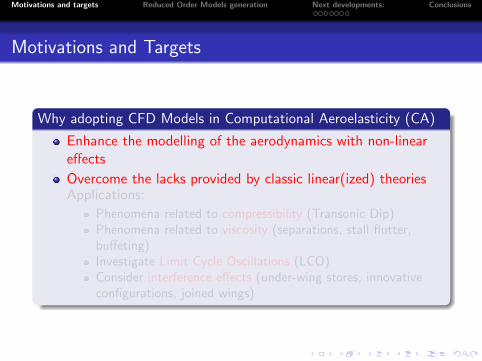
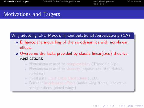
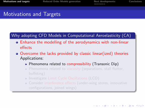
Motivations and Targets
Why adopting CFD Models in Computational Aeroelasticity (CA)
Enhance the modelling of the aerodynamics with non-lineareffects
Overcome the lacks provided by classic linear(ized) theoriesApplications:
Phenomena related to compressibility (Transonic Dip)Phenomena related to viscosity (separations, stall flutter,buffeting)Investigate Limit Cycle Oscillations (LCO)Consider interference effects (under-wing stores, innovativeconfigurations, joined wings)
Motivations and targets Reduced Order Models generation Next developments: Conclusions
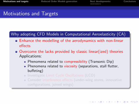
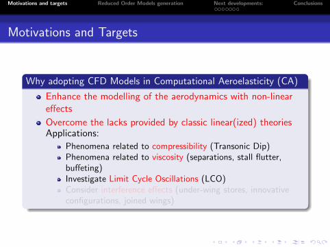
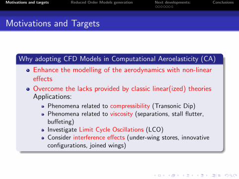
Motivations and Targets
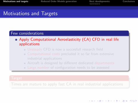
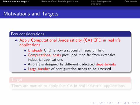
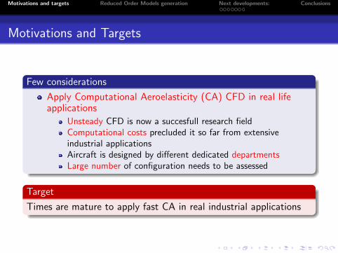
Few considerations
Apply Computational Aeroelasticity (CA) CFD in real lifeapplications
Unsteady CFD is now a succesfull research fieldComputational costs precluded it so far from extensiveindustrial applicationsAircraft is designed by different dedicated departmentsLarge number of configuration needs to be assessed
Target
Times are mature to apply fast CA in real industrial applications

Motivations and targets Reduced Order Models generation Next developments: Conclusions
Motivations and Targets
Few considerations
Apply Computational Aeroelasticity (CA) CFD in real lifeapplications
Unsteady CFD is now a succesfull research fieldComputational costs precluded it so far from extensiveindustrial applicationsAircraft is designed by different dedicated departmentsLarge number of configuration needs to be assessed
Target
Times are mature to apply fast CA in real industrial applications
Motivations and targets Reduced Order Models generation Next developments: Conclusions
Outline
1 Motivations and targets
2 Reduced Order Models generation
3 Transpiration Method
4 Next developments:Spatial coupling: MLS TechniqueMultibody coupling: MBDyn
5 Conclusions
Motivations and targets Reduced Order Models generation Next developments: Conclusions
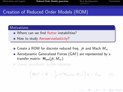
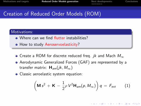
Creation of Reduced Order Models (ROM)
Motivations:
Where can we find flutter instabilities?
How to study Aeroservoelasticity?
Create a ROM for discrete reduced freq. jk and Mach M∞
Aerodynamic Generalized Forces (GAF) are represented by atransfer matrix: Ham(jk,M∞)
Classic aeroelastic system equation:(M s2 + K − 1
2ρ V 2Ham(p,M∞)
)q = Fext (1)

Motivations and targets Reduced Order Models generation Next developments: Conclusions
Creation of Reduced Order Models (ROM)
Motivations:
Where can we find flutter instabilities?
How to study Aeroservoelasticity?
Create a ROM for discrete reduced freq. jk and Mach M∞
Aerodynamic Generalized Forces (GAF) are represented by atransfer matrix: Ham(jk,M∞)
Classic aeroelastic system equation:(M s2 + K − 1
2ρ V 2Ham(p,M∞)
)q = Fext (1)
Motivations and targets Reduced Order Models generation Next developments: Conclusions
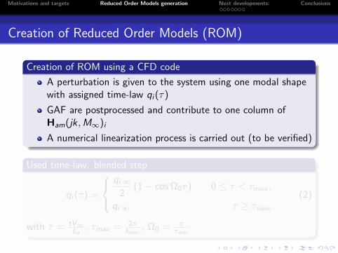
Creation of Reduced Order Models (ROM)
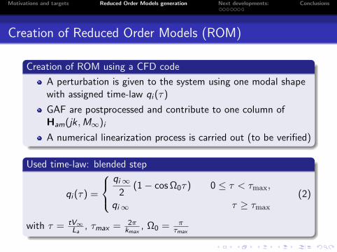
Creation of ROM using a CFD code
A perturbation is given to the system using one modal shapewith assigned time-law qi (τ)
GAF are postprocessed and contribute to one column ofHam(jk,M∞)i
A numerical linearization process is carried out (to be verified)
Used time-law: blended step
qi (τ) =
qi∞2
(1− cos Ω0τ) 0 ≤ τ < τmax,
qi∞ τ ≥ τmax
(2)
with τ = tV∞La
, τmax = 2πkmax
, Ω0 = πτmax
Motivations and targets Reduced Order Models generation Next developments: Conclusions
Creation of Reduced Order Models (ROM)
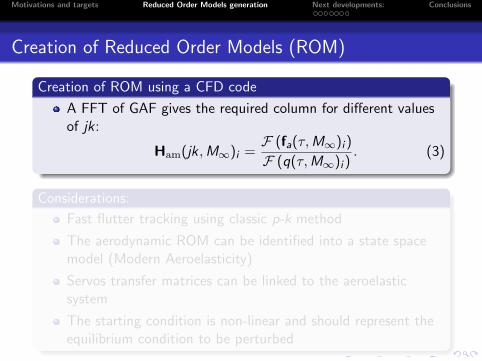
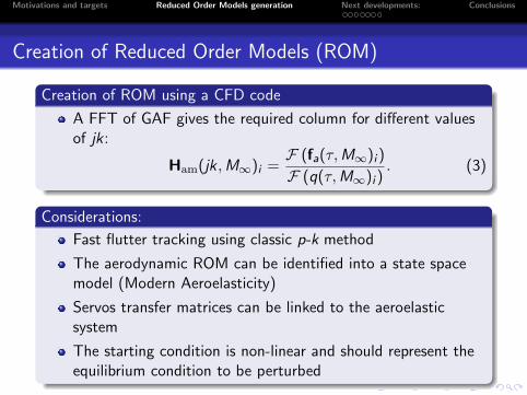
Creation of ROM using a CFD code
A FFT of GAF gives the required column for different valuesof jk:
Ham(jk,M∞)i =F (fa(τ,M∞)i )
F (q(τ,M∞)i ). (3)
Considerations:
Fast flutter tracking using classic p-k method
The aerodynamic ROM can be identified into a state spacemodel (Modern Aeroelasticity)
Servos transfer matrices can be linked to the aeroelasticsystem
The starting condition is non-linear and should represent theequilibrium condition to be perturbed
Motivations and targets Reduced Order Models generation Next developments: Conclusions
Creation of Reduced Order Models (ROM)
Creation of ROM using a CFD code
A FFT of GAF gives the required column for different valuesof jk:
Ham(jk,M∞)i =F (fa(τ,M∞)i )
F (q(τ,M∞)i ). (3)
Considerations:
Fast flutter tracking using classic p-k method
The aerodynamic ROM can be identified into a state spacemodel (Modern Aeroelasticity)
Servos transfer matrices can be linked to the aeroelasticsystem
The starting condition is non-linear and should represent theequilibrium condition to be perturbed
Motivations and targets Reduced Order Models generation Next developments: Conclusions
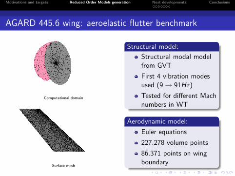
AGARD 445.6 wing: aeroelastic flutter benchmark
Computational domain
Surface mesh
Structural model:
Structural modal modelfrom GVT
First 4 vibration modesused (9 → 91Hz)
Tested for different Machnumbers in WT
Aerodynamic model:
Euler equations
227.278 volume points
86.371 points on wingboundary
Motivations and targets Reduced Order Models generation Next developments: Conclusions
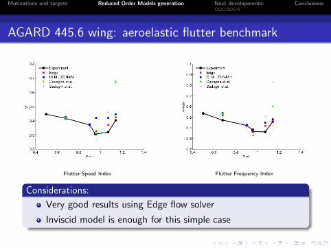
AGARD 445.6 wing: aeroelastic flutter benchmark
Flutter Speed Index Flutter Frequency Index
Considerations:
Very good results using Edge flow solver
Inviscid model is enough for this simple case
Motivations and targets Reduced Order Models generation Next developments: Conclusions
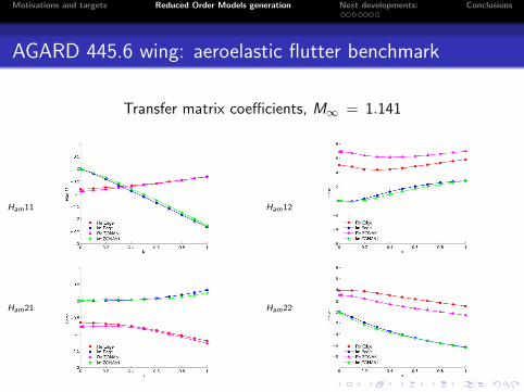
AGARD 445.6 wing: aeroelastic flutter benchmark
Transfer matrix coefficients, M∞ = 1.141
Ham11
Ham21
Ham12
Ham22
Motivations and targets Reduced Order Models generation Next developments: Conclusions
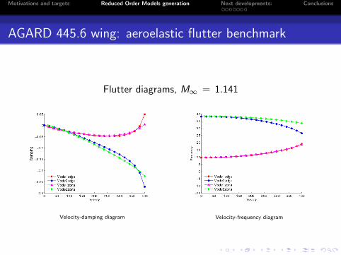
AGARD 445.6 wing: aeroelastic flutter benchmark
Flutter diagrams, M∞ = 1.141
Velocity-damping diagram Velocity-frequency diagram
Motivations and targets Reduced Order Models generation Next developments: Conclusions
Outline
1 Motivations and targets
2 Reduced Order Models generation
3 Transpiration Method
4 Next developments:Spatial coupling: MLS TechniqueMultibody coupling: MBDyn
5 Conclusions
Motivations and targets Reduced Order Models generation Next developments: Conclusions
Transpiration method
Advantages:
Simulate domain changes without updating the domain
Applications:
Classic panel methods to modify thickness by sources
Boundary layer patching with inviscid models
Multi Disciplinar Optimization
Aeroservoelasticity
Motivations and targets Reduced Order Models generation Next developments: Conclusions
Transpiration method
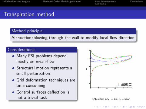
Method principle:
Air suction/blowing through the wall to modify local flow direction
Considerations:
Many FSI problems dependmostly on mean-flow
Structural motion represents asmall perturbation
Grid deformation techniques aretime-consuming
Control surfaces deflection isnot a trivial task RAE airfoil, M∞ = 0.3, α = 5deg
Motivations and targets Reduced Order Models generation Next developments: Conclusions
Transpiration method
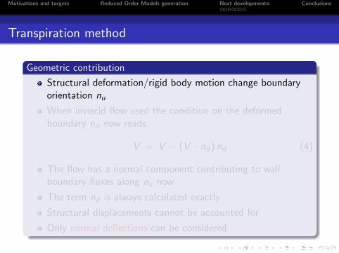
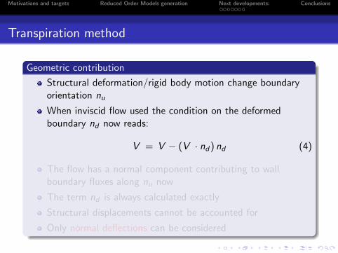
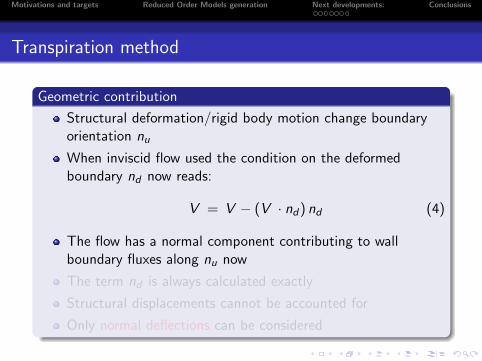
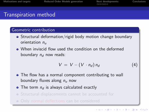
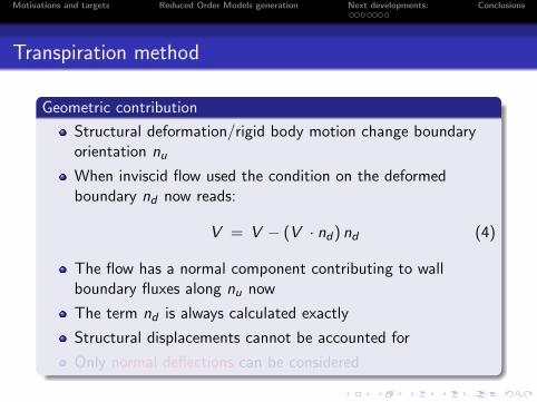
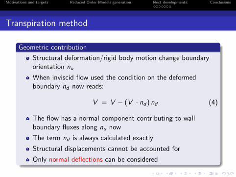
Geometric contribution
Structural deformation/rigid body motion change boundaryorientation nu
When inviscid flow used the condition on the deformedboundary nd now reads:
V = V − (V · nd) nd (4)
The flow has a normal component contributing to wallboundary fluxes along nu now
The term nd is always calculated exactly
Structural displacements cannot be accounted for
Only normal deflections can be considered
Motivations and targets Reduced Order Models generation Next developments: Conclusions
Transpiration method
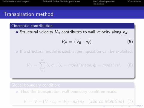
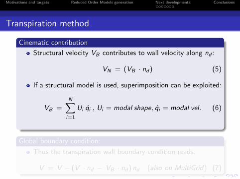
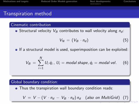
Cinematic contribution
Structural velocity VB contributes to wall velocity along nd :
VN = (VB · nd) (5)
If a structural model is used, superimposition can be exploited:
VB =N∑
i=1
Ui qi , Ui = modal shape, qi = modal vel . (6)
Global boundary condition:
Thus the transpiration wall boundary condition reads:
V = V − (V · nd − VB · nd) nd (also on MultiGrid) (7)
Motivations and targets Reduced Order Models generation Next developments: Conclusions
Transpiration method
Cinematic contribution
Structural velocity VB contributes to wall velocity along nd :
VN = (VB · nd) (5)
If a structural model is used, superimposition can be exploited:
VB =N∑
i=1
Ui qi , Ui = modal shape, qi = modal vel . (6)
Global boundary condition:
Thus the transpiration wall boundary condition reads:
V = V − (V · nd − VB · nd) nd (also on MultiGrid) (7)
Motivations and targets Reduced Order Models generation Next developments: Conclusions
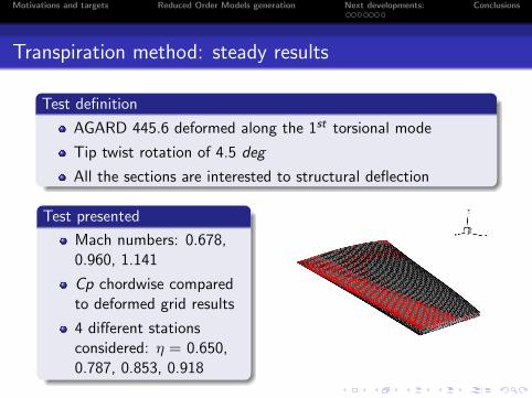
Transpiration method: steady results
Test definition
AGARD 445.6 deformed along the 1st torsional mode
Tip twist rotation of 4.5 deg
All the sections are interested to structural deflection
Test presented
Mach numbers: 0.678,0.960, 1.141
Cp chordwise comparedto deformed grid results
4 different stationsconsidered: η = 0.650,0.787, 0.853, 0.918
Motivations and targets Reduced Order Models generation Next developments: Conclusions
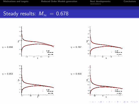
Steady results: M∞ = 0.678
η = 0.650
η = 0.853
η = 0.787
η = 0.918
Motivations and targets Reduced Order Models generation Next developments: Conclusions
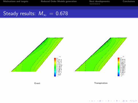
Steady results: M∞ = 0.678
Exact Transpiration
Motivations and targets Reduced Order Models generation Next developments: Conclusions
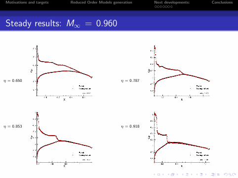
Steady results: M∞ = 0.960
η = 0.650
η = 0.853
η = 0.787
η = 0.918
Motivations and targets Reduced Order Models generation Next developments: Conclusions
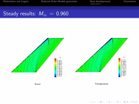
Steady results: M∞ = 0.960
Exact Transpiration
Motivations and targets Reduced Order Models generation Next developments: Conclusions
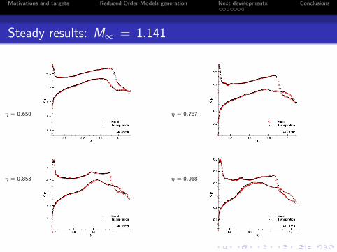
Steady results: M∞ = 1.141
η = 0.650
η = 0.853
η = 0.787
η = 0.918
Motivations and targets Reduced Order Models generation Next developments: Conclusions
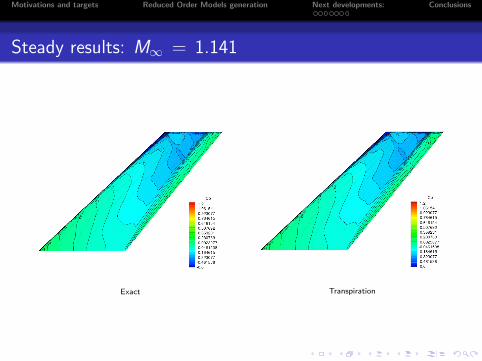
Steady results: M∞ = 1.141
Exact Transpiration
Motivations and targets Reduced Order Models generation Next developments: Conclusions
Outline
1 Motivations and targets
2 Reduced Order Models generation
3 Transpiration Method
4 Next developments:Spatial coupling: MLS TechniqueMultibody coupling: MBDyn
5 Conclusions
Motivations and targets Reduced Order Models generation Next developments: Conclusions
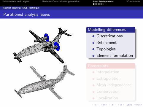
Spatial coupling: MLS Technique
Partitioned analysis issues
Modelling differences
Discretizations
Refinement
Topologies
Element formulation
Constraints
Interpolation
Extrapolation
Mesh independence
Conservation
Localization
Motivations and targets Reduced Order Models generation Next developments: Conclusions
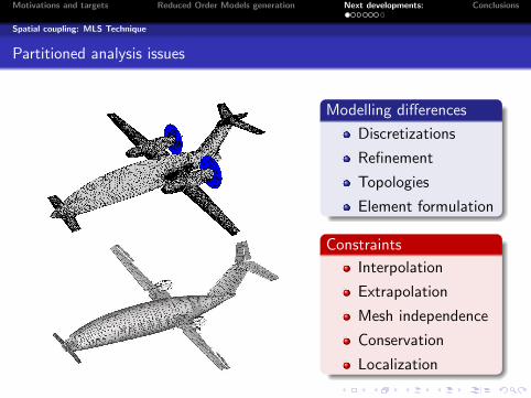
Spatial coupling: MLS Technique
Partitioned analysis issues
Modelling differences
Discretizations
Refinement
Topologies
Element formulation
Constraints
Interpolation
Extrapolation
Mesh independence
Conservation
Localization
Motivations and targets Reduced Order Models generation Next developments: Conclusions
Spatial coupling: MLS Technique
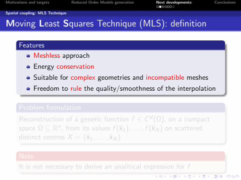
Moving Least Squares Technique (MLS): definition
Features
Meshless approach
Energy conservation
Suitable for complex geometries and incompatible meshes
Freedom to rule the quality/smoothness of the interpolation
Problem formulation
Reconstruction of a generic function f ∈ Cd(Ω), on a compactspace Ω ⊆ Rn, from its values f (x1), . . . , f (xN) on scattereddistinct centres X = x1, . . . , xN
Note
It is not necessary to derive an analitical expression for f
Motivations and targets Reduced Order Models generation Next developments: Conclusions
Spatial coupling: MLS Technique
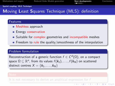
Moving Least Squares Technique (MLS): definition
Features
Meshless approach
Energy conservation
Suitable for complex geometries and incompatible meshes
Freedom to rule the quality/smoothness of the interpolation
Problem formulation
Reconstruction of a generic function f ∈ Cd(Ω), on a compactspace Ω ⊆ Rn, from its values f (x1), . . . , f (xN) on scattereddistinct centres X = x1, . . . , xN
Note
It is not necessary to derive an analitical expression for f

Motivations and targets Reduced Order Models generation Next developments: Conclusions
Spatial coupling: MLS Technique
Moving Least Squares Technique (MLS): definition
Features
Meshless approach
Energy conservation
Suitable for complex geometries and incompatible meshes
Freedom to rule the quality/smoothness of the interpolation
Problem formulation
Reconstruction of a generic function f ∈ Cd(Ω), on a compactspace Ω ⊆ Rn, from its values f (x1), . . . , f (xN) on scattereddistinct centres X = x1, . . . , xN
Note
It is not necessary to derive an analitical expression for f
Motivations and targets Reduced Order Models generation Next developments: Conclusions
Spatial coupling: MLS Technique
Moving Least Squares Technique (MLS): conservation
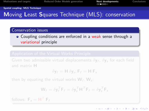
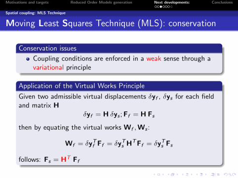
Conservation issues
Coupling conditions are enforced in a weak sense through avariational principle
Application of the Virtual Works Principle
Given two admissible virtual displacements δyf , δys for each fieldand matrix H
δyf = H δys ;Ff = H Fs
then by equating the virtual works Wf ,Ws :
Wf = δyTf Ff = δyT
s HTFf = δyTs Fs
follows: Fs = HT Ff
Motivations and targets Reduced Order Models generation Next developments: Conclusions
Spatial coupling: MLS Technique
Moving Least Squares Technique (MLS): conservation
Conservation issues
Coupling conditions are enforced in a weak sense through avariational principle
Application of the Virtual Works Principle
Given two admissible virtual displacements δyf , δys for each fieldand matrix H
δyf = H δys ;Ff = H Fs
then by equating the virtual works Wf ,Ws :
Wf = δyTf Ff = δyT
s HTFf = δyTs Fs
follows: Fs = HT Ff
Motivations and targets Reduced Order Models generation Next developments: Conclusions
Spatial coupling: MLS Technique
Moving Least Squares Technique (MLS): approximation
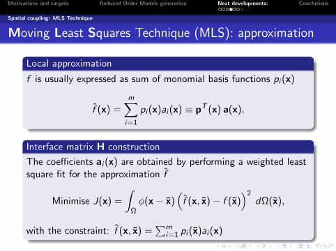
Local approximation
f is usually expressed as sum of monomial basis functions pi (x)
f (x) =m∑
i=1
pi (x)ai (x) ≡ pT (x) a(x),
Interface matrix H construction
The coefficients ai (x) are obtained by performing a weighted leastsquare fit for the approximation f
Minimise J(x) =
∫Ω
φ(x− x)(f (x, x)− f (x)
)2dΩ(x),
with the constraint: f (x, x) =∑m
i=1 pi (x)ai (x)
Motivations and targets Reduced Order Models generation Next developments: Conclusions
Spatial coupling: MLS Technique
Moving Least Squares Technique (MLS): localization
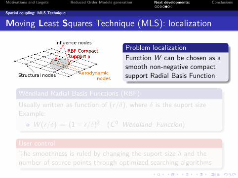
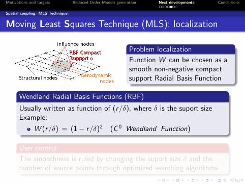
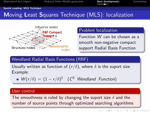
Problem localization
Function W can be chosen as asmooth non-negative compactsupport Radial Basis Function
Wendland Radial Basis Functions (RBF)
Usually written as function of (r/δ), where δ is the suport sizeExample:
W (r/δ) = (1− r/δ)2 (C 0 Wendland Function)
User control
The smoothness is ruled by changing the suport size δ and thenumber of source points through optimized searching algorithms
Motivations and targets Reduced Order Models generation Next developments: Conclusions
Spatial coupling: MLS Technique
Moving Least Squares Technique (MLS): localization
Problem localization
Function W can be chosen as asmooth non-negative compactsupport Radial Basis Function
Wendland Radial Basis Functions (RBF)
Usually written as function of (r/δ), where δ is the suport sizeExample:
W (r/δ) = (1− r/δ)2 (C 0 Wendland Function)
User control
The smoothness is ruled by changing the suport size δ and thenumber of source points through optimized searching algorithms
Motivations and targets Reduced Order Models generation Next developments: Conclusions
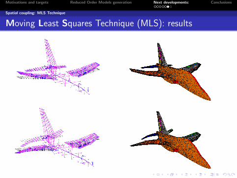
Spatial coupling: MLS Technique
Moving Least Squares Technique (MLS): results
Motivations and targets Reduced Order Models generation Next developments: Conclusions
Multibody coupling: MBDyn
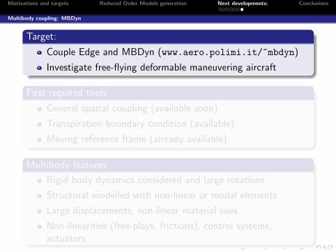
Target:
Couple Edge and MBDyn (www.aero.polimi.it/~mbdyn)
Investigate free-flying deformable maneuvering aircraft
First required tools:
General spatial coupling (available soon)
Transpiration boundary condition (available)
Moving reference frame (already available)
Multibody features:
Rigid body dynamics considered and large rotations
Structural modelled with non-linear or modal elements
Large displacements, non-linear material laws
Non-linearities (free-plays, frictions), control systems,actuators

Motivations and targets Reduced Order Models generation Next developments: Conclusions
Multibody coupling: MBDyn
Target:
Couple Edge and MBDyn (www.aero.polimi.it/~mbdyn)
Investigate free-flying deformable maneuvering aircraft
First required tools:
General spatial coupling (available soon)
Transpiration boundary condition (available)
Moving reference frame (already available)
Multibody features:
Rigid body dynamics considered and large rotations
Structural modelled with non-linear or modal elements
Large displacements, non-linear material laws
Non-linearities (free-plays, frictions), control systems,actuators
Motivations and targets Reduced Order Models generation Next developments: Conclusions
Outline
1 Motivations and targets
2 Reduced Order Models generation
3 Transpiration Method
4 Next developments:Spatial coupling: MLS TechniqueMultibody coupling: MBDyn
5 Conclusions
Motivations and targets Reduced Order Models generation Next developments: Conclusions
Conclusion and future developments
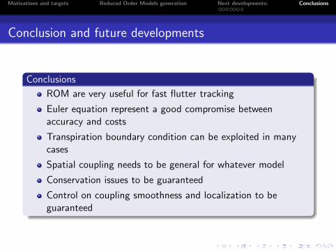
Conclusions
ROM are very useful for fast flutter tracking
Euler equation represent a good compromise betweenaccuracy and costs
Transpiration boundary condition can be exploited in manycases
Spatial coupling needs to be general for whatever model
Conservation issues to be guaranteed
Control on coupling smoothness and localization to beguaranteed
Motivations and targets Reduced Order Models generation Next developments: Conclusions
Acknowledgments
Jonathan Smith, FOI
Peter Eliasson, FOI
References
L. Cavagna, G. Quaranta, and P. Mantegazza
Application of Navier-Stokes simulations for aeroelastic assessmentin transonic regime
Computers & Structures, vol. 85, no. 11-14, pp. 818–832, 2007.
L. Cavagna, G. Quaranta, P. Mantegazza, and D. Marchetti
Aeroelastic assessment of the free flying aircraft in transonic regime
International Forum on Aeroelasticity and Structural DynamicsIFASD-2007, (Stochkolm, Sweden), June 18-20, 2007.
G. Quaranta, P. Masarati, and P. Mantegazza
A conservative mesh-free approach for fluid-structure interfaceproblems
International Conference on Computational Methods for CoupledProblems in Science and Engineering (M. Papadrakakis, E. Onate,and B. Schrefler, eds.), (Santorini, Greece), CIMNE, 2005.
Towards a Comprehensive Environment forAeroservoelastic analysis in Edge flow solver
L. Cavagna, P. Masarati, G. Quaranta and P. Mantegazza
Dipartimento di Ingegneria Aerospaziale, Politecnico di Milano
November 15, 2007FOI Swedish Defence Agency, Kista - Stockholm