Totalflow Plunger Analysis Software - ABB · PDF file1.2 Plunger Analysis Software Background...

2104207-001– rev. AA

Totalflow® Plunger Analysis Software User’s Manual

XRCG4

Intellectual Property & Copyright Notice

©2010 by ABB Inc., Totalflow (“Owner”), Bartlesville, Oklahoma 74006, U.S.A. All rights reserved. Any and all derivatives of, including translations thereof, shall remain the sole property of the Owner, regardless of any circumstances. The original US English version of this manual shall be deemed the only valid version. Translated versions, in any other language, shall be maintained as accurately as possible. Should any discrepancies exist, the US English version will be considered final. Notice: This publication is for information only. The contents are subject to change without notice and should not be construed as a commitment, representation, warranty, or guarantee of any method, product, or device by Owner. Inquiries regarding this manual should be addressed to ABB Inc., Totalflow Products, Technical Communications, 7051 Industrial Blvd., Bartlesville, Oklahoma 74006, U.S.A.

i

TABLE OF CONTENTS INTRODUCTION ...................................................................................................... III

Organization & Style....................................................................................................iii Chapter Descriptions...................................................................................................iii Getting Help ................................................................................................................iii

Before Calling ...............................................................................................................iii Key Symbols .............................................................................................................. iv Safety Practices and Precautions .............................................................................. iv

Equipment Markings.....................................................................................................iv Grounding the Product .................................................................................................iv Operating Voltage.........................................................................................................iv Danger From Loss of Ground.......................................................................................iv Safety First ................................................................................................................... v Equipment Markings..................................................................................................... v Grounding the Product ................................................................................................. v Operating Voltage......................................................................................................... v Danger From Loss of Ground....................................................................................... v Safe Equipment ............................................................................................................vi

1.0 DESCRIPTION................................................................................................ 7 1.1 Plunger Lift Background .................................................................................. 7 1.2 Plunger Analysis Software Background .......................................................... 7 1.3 Modes.............................................................................................................. 8

1.3.1 Batch................................................................................................................ 8 1.3.2 Graphical User Interface (GUI)........................................................................ 8

2.0 INSTALLATION.............................................................................................. 8 2.1 Software Installation ........................................................................................ 8

3.0 TREND FILE SETUP FOR TOTALFLOW XSERIES UNITS.......................... 9 3.1 Creating a Trend File..................................................................................... 10

3.1.1 Adding A Variable.......................................................................................... 14 3.1.2 Loading the Trend File................................................................................... 16

4.0 COLLECTING TREND FILES FOR INPUT INTO THE SOFTWARE ........... 17 4.1 Converting to CSV File .................................................................................. 20

5.0 IMPORTING DATA FILES INTO THE SOFTWARE..................................... 22 5.1 Data Integrity Filters ...................................................................................... 22 5.2 Importing Data from a .CSV File.................................................................... 24

6.0 VIEWING PLUNGER SETTINGS ................................................................. 27 7.0 PLUNGER ANALYSIS SOFTWARE TABS ................................................. 28

7.1 Plunger Timing Tab ....................................................................................... 28 7.2 Multi Flow Rate Tab....................................................................................... 29 7.3 Multi Flow Rate Overlay Tab ......................................................................... 29 7.4 Single Flow and Pressure Tab ...................................................................... 30 7.5 Single Shut-In Tab......................................................................................... 31

ii

7.6 Mult Shut-In Tab............................................................................................ 32 7.7 Valve Open Tab ............................................................................................ 33 7.8 Single Slug Size Tab ..................................................................................... 33 7.9 Multi Slug Size Tab ....................................................................................... 34 7.10 Slug Size Tab ................................................................................................ 35 7.11 Load Factor Tab ............................................................................................ 35

TABLE OF FIGURES

Figure 3–1 Remote Communications Tab ............................................................................................10 Figure 3–2 Trend System Tab ..............................................................................................................11 Figure 3–3 Configure Device Trend Dialog Box ...................................................................................11 Figure 3–4 Trend File Configuration Dialog Box...................................................................................12 Figure 3–5 Trend File Configuration .....................................................................................................13 Figure 3–6 Trend Variable Configuration Dialog Box ...........................................................................14 Figure 3–7 Trend Variable Configuration – Snapshot ..........................................................................15 Figure 3–8 Trend File Configuration – Send to Device.........................................................................16 Figure 3–9 Configure Device Trend Dialog Box ...................................................................................17 Figure 4–1 Device Trend Dialog Box ....................................................................................................18 Figure 4–2 Device Trend Dialog Box – Path.........................................................................................18 Figure 4–3 Trend File – Line Graph......................................................................................................19 Figure 4–4 Trend File – Tabular Data...................................................................................................20 Figure 4–5 PCCU32 Window................................................................................................................21 Figure 4–6 PLTrend Folder ...................................................................................................................21 Figure 5–1 Plunger Analysis Software Home Screen...........................................................................22 Figure 5–2 Plunger Analysis Software Options Dialog Box..................................................................23 Figure 5–3 Select Data Columns Dialog Box........................................................................................25 Figure 5–4 Well Configuration Dialog Box ............................................................................................26 Figure 5–5 Trend Data Tab...................................................................................................................26 Figure 6–1 Plunger Settings Tab ..........................................................................................................27 Figure 7–1 Plunger Timing Tab ............................................................................................................28 Figure 7–2 Multi Flow Rate Tab............................................................................................................29 Figure 7–3 Multi Flow Rate Overlay......................................................................................................30 Figure 7–4 Single Flow and Pressure Tab............................................................................................30 Figure 7–5 Single Shut-In Tab ..............................................................................................................31 Figure 7–6 Multi Shut-In Tab.................................................................................................................32 Figure 7–7 Valve Open Tab..................................................................................................................33 Figure 7–8 Single Slug Size Tab ..........................................................................................................34 Figure 7–9 Multi Slug Size Tab.............................................................................................................34 Figure 7–10 Slug Size Tab....................................................................................................................35 Figure 7–11 Load Factor Tabs..............................................................................................................36

iii

Introduction The following manual is written to provide information regarding the Totalflow Plunger Analysis Software.

Organization & Style Each of the chapters in this manual presents information in an organized and concise manner. Readers are able to look at the headings and get a broad picture of the content without reading every word. Also, there are overviews at the beginning of each chapter that provides the user with an idea of what is in the chapter and how it fits into the overall manual.

Chapter Descriptions The following presents a breakdown of each individual chapter. Chapter Name Description

1 Introduction Provides a brief overview of the Plunger Analysis Software.

2 Installation Provides instructions on installing the Plunger Analysis Software.

3 Trend File Setup Includes information on establishing the trend file.

4 Trend File Collection

Provides the user with information on trend file collection to include local and remote connect.

5 Importing Data into the Plunger Analysis Software

Provides information on how to import data into the Plunger Analysis Software.

6 Plunger Analysis Software Settings

Provides a description of the analysis software settings.

7 Plunger Analysis Software Tabs

Provides a description of the various tabs that the user will encounter within the Plunger Analysis Software.

Getting Help Totalflow takes pride in the ongoing support provided to our customers. When purchasing a product, the user receives documentation which should answer their questions; however, Totalflow Technical Support provides an 800 number as an added source of information.

If requiring assistance, call:

USA: (800) 442-3097 International: 001-918-338-4888

Before Calling • Be prepared to give the customer service representative a detailed

description of the problem. • Note any alarms or messages as they appear. • Prepare a written description of the problem. • Know the software version, board and optional part numbers.

iv

Key Symbols The following symbols are used frequently in the manual. These are intended to catch the eye and draw attention to important information.

Intended to draw attention to useful information or to clarify a statement made earlier.

Intended to draw attention to a fact that may be useful or helpful in understanding a concept.

Intended to draw attention to a statement that might keep the user from making a mistake, keep them from destroying equipment or parts or keep them from creating a situation that could cause personal injury if caution is not used. Please refer to the Safety Practices and Precaution section for additional information.

Intended to draw attention to a statement regarding the likelihood of personal injury or fatality that could result from improper access or techniques used while working in hazardous locations. Please refer to the Safety Practices and Precaution section for additional information.

Safety Practices and Precautions This manual contains information and warnings which have to be followed by the user to ensure safe operation and to retain the product in a safe condition. Installation, maintenance and repairs should only be performed by a trained and qualified technician.

Equipment Markings

Protective ground (earth) terminal.

Grounding the Product

If a grounding conductor is required, it should be connected to the grounding terminal before any other connections are made.

Operating Voltage

Before switching on the power, check that the operating voltage listed on the equipment agrees with the power being connected to the equipment.

Danger From Loss of Ground

A grounding conductor may or may not be required depending on the hazardous classification. If required, any interruption of the grounding conductor inside or outside the equipment or loose connection of the grounding conductor can result in a dangerous unit. Intentional interruption of the grounding conductor is not permitted.

v

Safety First

Various statements in this manual, identified as conditions or practices that could result in equipment damage, personal injury or loss of life, will be highlighted using the following icons.

Exercise caution while performing this task. Carelessness could result in damage to the equipment, other property and personal injury.

STOP. Do not proceed without first verifying that a hazardous condition does not exist. This task may not be undertaken until proper protection has been accomplished, or the hazardous condition has been removed. Personal injury or fatality could result. Examples of these warnings include: • Removal of enclosure cover(s) in a hazardous location

must follow guidelines stipulated in the Certification Drawings shipped with this unit.

• If unit is installed or to be installed in a hazardous location, technician must follow the guidelines stipulated in the Certification Drawings shipped with this unit.

• Access to unit via PCCU cable in a hazardous location must follow guidelines stipulated in the Certification Drawings shipped with this unit.

• Connecting or disconnecting equipment in a hazardous location for installation or maintenance of electric components must follow guidelines stipulated in the Certification Drawings shipped with this unit.

WARNING indicates a personal injury hazard immediately accessible as one reads the markings. CAUTION indicates a personal injury hazard not immediately accessible as one reads the markings or a hazard to property including the equipment itself.

Equipment Markings

Protective ground (earth) terminal.

Grounding the Product

If a grounding conductor is required, it should be connected to the grounding terminal before any other connections are made.

Operating Voltage

Before switching on the power, check that the operating voltage listed on the equipment agrees with the power being connected to the equipment.

Danger From Loss of Ground

A grounding conductor may or may not be required depending on the hazardous classification. If required, any interruption of the grounding conductor inside or outside the equipment or loose connection of the grounding conductor can result

vi

in a dangerous unit. Intentional interruption of the grounding conductor is not permitted.

Safe Equipment

If it is determined that the equipment cannot be operated safely, it should be taken out of operation and secured against unintentional usage.

2104207-001 rev. AA Page 7

1.0 DESCRIPTION

1.1 Plunger Lift Background The Plunger Lift application works in a manner similar to a pneumatic piston, wherein it is caused by gravity to fall to the bottom of a well. Acting as a seal between the liquid and gas, the plunger settles to the bottom of the production tubing and allows liquid to accumulate above it. This accumulation of liquid restricts the flow of gas and slows it down. The production valve is closed to allow down-hole pressure to build in the casing. After the pressure has built, the production valve is opened, and the casing pressure lifts the plunger and accumulated liquids to the surface. At the surface, separators remove the liquids from the gas. Once the volume of the flowing gas drops, it becomes necessary to choose a time or method of closing the production valve. Once closed, the plunger drops to the bottom of the production tube. With the plunger deployed and the well shut-in, the down-hole pressure builds, and the cycle is repeated.

The entire operation takes place by the simple expediency of opening or closing a valve. There are many options available for determining when to open and close the valve, and these options can then be used to modify the plunger to optimize well production.

1.2 Plunger Analysis Software Background ABB Totalflow has developed an application that will help the user better understand how to fully use the Totalflow Plunger system that is available in all XSeries (8-bit and 32-bit) units. This tool is a stand alone application that analyzes plunger lift cycles via trend files and calculates set points based on averages and other statistical data. This user’s manual and corresponding illustrations are specifically geared towards the 8-bit (G3) XSeries user, but all of the operations shown within the manual can be modified easily to perform with the 32-bit (G4) products. The Totalflow Plunger system has many available open and close parameters which can be modified for the maximum optimization of well production. This complexity, along with the myriad of ways in which to run a plunger, often leaves the user with a level of confusion on where to start running their plunger system. As such, the following instructions, used in conjunction with the Plunger Analysis Software, will provide a means for the user to gather and display data that will be helpful in the successful operation of a plunger system with an XSeries Totalflow controller. The user’s guide is aimed at XSeries users who are familiar with setting up and collecting trend files, either locally or remotely. As previously outlined, the user’s manual will walk the user through setting up the trend file necessary to collect the data that is needed by the Plunger Analysis Software, ways to save the data for importing into the software, importing the data itself, analyzing the data, saving and printing reports from the analysis.

Currently, this program can only function properly if ALL trending data points are available. Particularly, the program WILL NOT calculate correctly when data from a PACKER WELL is used.

2104207-001 rev. AA Page 8

For additional help, contact ABB Totalflow technical support with questions regarding the Plunger Analysis Software.

If requiring assistance, call: USA: (800) 442-3097 or International: 001-918-338-4888

1.3 Modes

1.3.1 Batch

The standard application can be run as a batch service if that service has been purchased. Command line parameters are passed when calling the executable. The batch service will analyze the entire plunger lift trend .*csv’s in a particular directory. The output will be recommended set point settings and other statistical data relevant for each well analyzed.

1.3.2 Graphical User Interface (GUI)

This is the default mode. When the executable is double clicked the standard graphical user interface is displayed and a *.csv file will need to be manually loaded via the toolbar or menu bar.

2.0 INSTALLATION The following information will detail the steps necessary for the user to install the Plunger Analysis Software onto their computer. It is assumed that the user has purchased the software and has received the software disk and software key before beginning the installation process.

2.1 Software Installation The following assumes that the user is installing the Plunger Analysis Software onto their computer for the first time.

1) Load the Totalflow application disk in the PC’s CD/DVD drive. The disk will initialize. Once completed, the Totalflow Plunger Analysis Software screen displays. Click the Modify radio button to install the new application onto the user’s computer.

2) Click the Next button.

3) The Select Features window displays. Ensure the Default Feature box is checked, and click the Next button.

4) The program will begin loading. When it has completed, click the Finish button.

5) When the User Information dialog box displays, the user needs to enter their name and their company’s name. In the Serial Number field, type in the serial number associated with the user’s version of the Plunger Analysis Software. The serial number is printed on an insert inside the sealed envelope that contains the software disk. Click Next.

When typing in the serial number, the user needs to ensure that the number is typed exactly as it appears on the printed sheet to include dashes (-).

6) This will complete the installation process for the Plunger Analysis Software.

2104207-001 rev. AA Page 9

3.0 TREND FILE SETUP FOR TOTALFLOW XSERIES UNITS There is specific information that needs to be collected from a Totalflow XSeries unit that is then consequently provided to the Plunger Analysis Software for analysis. In this section, the user will be shown instructions on how to set up the correct trend to gather this information and how to calculate the amount of data that the user will need.

In general, the user will be trending five individual points of information using a specific time interval that will allow for enough time to gather a minimum of ten complete (from start of the closed cycle to the end of the after flow cycle) plunger cycles based on the setup parameters of the unit.

The information that needs to be collected for the trend file are: • Casing Pressure • Tubing Pressure • Line Pressure • Flow Rate • Arrival Time

Prior to starting the creation of the trend file, the user will need to record the app.array.register for each of the individual information components (bulleted list above) that will be added to the trend. Typically, the casing and tubing pressures are being brought into the unit via analog inputs either onboard or on a TFIO AI module. These are then subsequently defined in the Plunger application as inputs at 18.101.26 for casing and 18.101.16 for tubing (described in the Plunger application as Ext Pressure AI).

Depending on the location of the valve and the Plunger setup, either upstream or downstream, the tubing pressure may be the SP register from the Tube application. Typical setup is for the valve to be upstream, and the Ext Pressure AI will be used for tubing pressure.

The line pressure for the Upstream Valve setup would come from the static pressure reading of the Tube application at 11.3.0, or if a Downstream Valve setup, it would come from an external AI. The flow rate is usually taken from the Tube application at register 11.7.19. The Arrival Time is taken from the Statistics > Plunger Arrivals from the Plunger application and is the most current arrival time from register 18.104.23.

The following illustrations will walk the user through creating the trend file that will be the input data from the meter to the Plunger Analysis Software.

The user must insure that the Flash they are using is an 8-bit or 32-bit XSeries meter supporting Trend files. If not, the user will need to upgrade their Flash to a version that does support trends. In 32-bit XSeries devices, the user will need to insure they have enough available application credits to be able to instantiate the Trend System application.

2104207-001 rev. AA Page 10

3.1 Creating a Trend File 1) Connect to the meter, and verify that the Trend System is instantiated. If not

instantiated, the user will need to move to the Applications tab, and instantiate the application. This is done in slot 21 for the 8-bit device and slot 95 for the 32-bit device.

2) After the user has instantiated the Trend System application, click the Local icon in the toolbar at the top of the PCCU window. This will take the user to the Remote Protocol screen (see Figure 3–1).

3) From the Remote Communications entry screen, click on the Trend System tab to access the area (see Figure 3–2). This is where the user will create and modify trends.

4) Within the Trend System tab, click on the Configure Device button. This will enable the user to read the contents of the device.

5) Once the contents of the device’s trend system are read into PCCU, the user will see a dialog box (see Figure 3–3) that details what is available. If any pre-existing trend files are in the unit, they will be able to view them in the Available Files section in the middle of the window. Additionally, note the available free space (in bytes). When creating trend files, the user does not want them to be larger than 50% of the available free space, or the user will not be able to collect the trend.

Figure 3–1 Remote Communications Tab

2104207-001 rev. AA Page 11

Figure 3–2 Trend System Tab

Figure 3–3 Configure Device Trend Dialog Box

6) Ensure that the Device File Path reflects the \TREND\ directory on the device. From this point on, the user will be ready to create the trend file that will record the information necessary for the Plunger Analysis Software to operate properly.

7) In the Configure Device Trend dialog box, click on the New button. This will enable the user to create the trend file. Upon clicking the button, the Trend File Configuration dialog box will display (see Figure 3–4).

2104207-001 rev. AA Page 12

8) Within the Trend File Configuration dialog box, the user will be able to perform the following actions:

• Define the file name.

• Give a description of the trend file.

• Enable the Scan Status (defaults to On).

• Define the Scan Period (or how often the user reads the data points).

• Define the Log Period (or how often the user logs values into the trend file).

• Define the Max Variables (the number of data points the user is trending).

• Define the Max Records (how many records determines the length and size).

• Define the Variables (the five data points necessary).

• Send the file to the device. In the following example, several of the bulleted items listed above have been completed. It should be noted that the File Name is limited to eight characters with more characters allotted for the description.

Figure 3–4 Trend File Configuration Dialog Box

In Figure 3–5, the granularity of the data is sufficient when the Scan Period is set to one minute, and the Log Period is set to five minutes. If more granularity is necessary for the user’s system, adjusting these scan and log periods can be edited, but doing so will cause some data irregularity until the file is completely rebuilt over the time period allotted via the Max Records. The amount of time covered by the trend file will be reduced accordingly. In this example, the data

2104207-001 rev. AA Page 13

points will be scanned once per minute, and at the end of every five minutes, the average of the previous five minutes will be logged into the trend file.

The process of deciding how many Max Records are needed can have many steps:

• First, the user will need to know the approximate average cycle time for their plunger system to complete one cycle.

• Secondly, the user will need to calculate the number of hours using the normal cycle time that it would take to record a minimum of ten complete cycles.

• Lastly, the user will need to calculate how many records it will take to cover the time period they have calculated to record the ten cycles. The user will need to keep in mind that they will want a 10-15% buffer to ensure they capture the amount of data needed and can round to the next highest whole number for simplicity. Ensure that this number of records will not cause the user to exceed 50% of the available space, or the user will not be able to collect the whole trend file in a single collect and could cause the user to have to collect only parts of the trend. Refer to the following diagram for an example of how to complete this setup.

Figure 3–5 Trend File Configuration

2104207-001 rev. AA Page 14

Sample Of How To Calculate Max Records

Typical complete plunger cycle time for example well:

90 minutes shut-in + 120 minute flow (including arrival time) = 210 Minutes total cycle time or (3 hours 30 minutes or 03:30:00)

Time required completing 10 cycles @ 03:30:00 per cycle

(210 minutes * 10 cycles)/60 minutes = 35 hours

Log period = 5 minutes; therefore, 12 logs per hour

(60 minutes / 5 minutes log = 12 logs per hour)

Figure the number of log periods needed to collect 10 cycles:

35 hours to collect 10 complete cycles * 12 logs per hour = 420 Log periods

420 Log periods * 10% buffer = 462 Log periods

For simplicity, round this to 500 Log periods)

For these items to complete, the user will need to set up each variable in the trend file.

3.1.1 Adding a Variable

1) To add a variable, click on the Add button in the Variable section of the Trend File Configuration dialog box. This will bring up the Trend Variable Configuration dialog box (see Figure 3–6). This is the area where the user can then define each variable.

Figure 3–6 Trend Variable Configuration Dialog Box

2104207-001 rev. AA Page 15

2) When configuring each variable, label each corresponding variable in the Description field. Typical engineering units for casing, tubing and line are PSIG or PSIA. These match the engineering units for flow rate to the setup for flow rate in the Tube application.

3) In the Variable section of the setup, input the appropriate app.array.register in the three defined areas.

4) The Trend Data section is where the user can define how to record the data. This trend needs to be set up to perform five minute averaging (refer to the Scan Period and Log Period definitions in the table above), so the default selection of Mean in the left most drop-down box is appropriate for the first four variables. As such, repeat this process for each variable.

5) Click the OK button at the completion of each variable setup.

6) Once the user has completed the setup for casing, tubing, line and flow, they will need to make one additional adjustment to record the Arrival Time correctly.

7) The arrival time needs to be a static number that is not averaged so that the data will reflect the correct amount of time it takes for the plunger to arrive on each cycle. The arrival time is displayed in the Plunger Statistics in hh:mm:ss format but is actually kept in seconds. As such, the appropriate engineering units are seconds. The change that is necessary to ensure that the user records the arrival time correctly in the trend file is located in the Trend Data section. The user will need to change how the data is recorded from Mean to Snapshot (see Figure 3–7). This means that when the Log Period occurs, this value will take a snapshot of the data value for the defined register and log that value rather than the average it is recording for the other four variables.

Figure 3–7 Trend Variable Configuration – Snapshot

2104207-001 rev. AA Page 16

3.1.2 Loading the Trend File

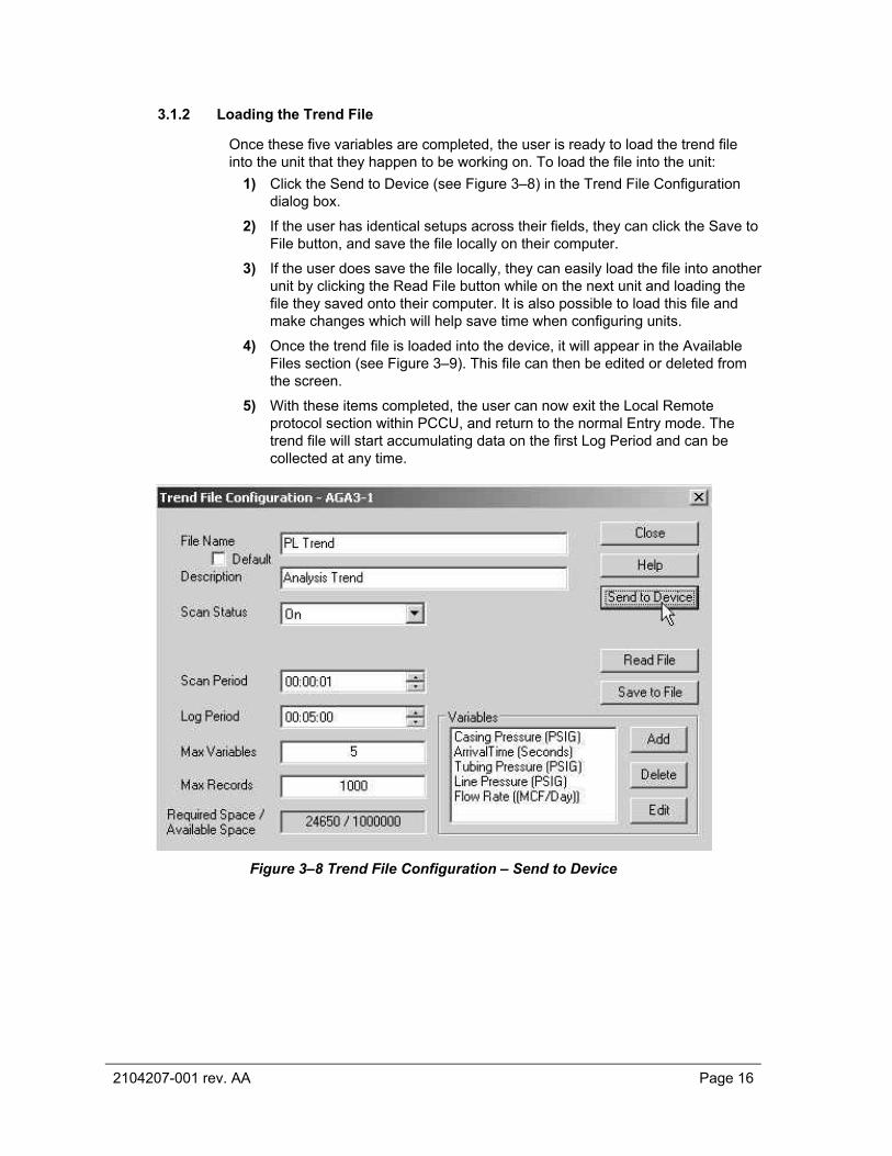
Once these five variables are completed, the user is ready to load the trend file into the unit that they happen to be working on. To load the file into the unit:

1) Click the Send to Device (see Figure 3–8) in the Trend File Configuration dialog box.

2) If the user has identical setups across their fields, they can click the Save to File button, and save the file locally on their computer.

3) If the user does save the file locally, they can easily load the file into another unit by clicking the Read File button while on the next unit and loading the file they saved onto their computer. It is also possible to load this file and make changes which will help save time when configuring units.

4) Once the trend file is loaded into the device, it will appear in the Available Files section (see Figure 3–9). This file can then be edited or deleted from the screen.

5) With these items completed, the user can now exit the Local Remote protocol section within PCCU, and return to the normal Entry mode. The trend file will start accumulating data on the first Log Period and can be collected at any time.

Figure 3–8 Trend File Configuration – Send to Device

2104207-001 rev. AA Page 17

Figure 3–9 Configure Device Trend Dialog Box

4.0 COLLECTING TREND FILES FOR INPUT INTO THE

SOFTWARE This chapter will detail the steps to collect the trend file that is necessary to gather the data to load into the analysis software. The user will be collecting the trend file via a local connection over the serial port and saving the output as a .csv (comma separated value) file, but the trend file can also be collected remotely via Totalflow WinCCU and other gathering systems.

1) Connect to PCCU, and start the application.

2) The user will then need to move into Entry mode. As before, the user will be using the Local Remote protocol to access the Trend System in the device (refer to section 3.0 for additional information on how to accomplish this).

3) Click on the Trend System tab in the Local Remote screen, and then click on Device Trend to access the Trend Directory on the device (see Figure 4–1).

4) The user will need to browse to the trend system on the unit by clicking the drop-down arrow within the Path field (see Figure 4–2) and selecting the trend they would like to download from the list displayed.

5) With the correct file trend selected from the drop-down list, the user can select the time range they would like to collect from. For the initial collect, and most likely for any subsequent collects, the user will want to select the All radio button. If this is not feasible, the user can then select either the Most Recent number of days or by defining a Date Range. If the user’s trend is too large to collect in a single poll, collecting by specific Date Range may prove to be a better method by which to access the needed data.

2104207-001 rev. AA Page 18

Figure 4–1 Device Trend Dialog Box

Figure 4–2 Device Trend Dialog Box – Path

2104207-001 rev. AA Page 19

6) The Output type most often used is to display the information to the screen, but the user might also want to log the output to a database for future reference. Whatever the option the user selects, click the corresponding radio button and then click the OK button.

7) Once this has been accomplished, the data will be collected and displayed back to the user in PCCU in a graphical format (see Figure 4–3). Additionally, the user is given the option to view the tabular data (see Figure 4–4) on the other tab.

As the user can view in Figure 4–4, the data is being logged in five minute intervals, as defined earlier in the manual when setting up the trend file. The trend file is a FIFO (first in – first out) file. This means that when the trend file fills up to the last record, the first record will be deleted to make room for the next most recent record. In this way, the user will always have the most up-to-date data in the file.

Figure 4–3 Trend File – Line Graph

2104207-001 rev. AA Page 20

Figure 4–4 Trend File – Tabular Data

4.1 Converting to CSV File The data being displayed on the screen needs to be converted into the .csv file, as referenced earlier.

1) Click on the Spreadsheet button at the bottom of the Trend File screen.

2) Once the file is created, the user will receive a confirmation pop-up window. Click the OK button, exit the Collection screen, the Local Remote section and then PCCU.

The directory in which the .csv file was created exists under the user’s PCCU32 installation directory (see Figure 4–5). This directory is placed within the C: drive. Using Windows Explorer, browse to the C: drive, and locate the PCCU32 directory. Once opened, locate the spreadsh folder, and then open it. In the folder there are at least two other folders, typically Longterm and Archive. The user will want to access the Archive folder and then look for a folder named after the trend the user created earlier. Inside this folder, the user will be able to locate the .csv file they created.

For the sake of simplicity, it is assumed that the folder is named PLTrend.

2104207-001 rev. AA Page 21

Figure 4–5 PCCU32 Window

Inside the PLTrend folder (see Figure 4–6), the user will find the .csv file that was created earlier. If the user is not familiar with meter IDs, they can find the file easily by using the Details view in Windows Explorer and searching for the file by the most recent date.

Figure 4–6 PLTrend Folder

The user may choose to move this file to a specific trend collection directory on their computer, or they can e-mail the .csv file to anyone whom might need it or rename the file to something more descriptive such as the well name or site name. This is the file the user will load into the Plunger Analysis Software, and depending on their corporate set up, they might have a central repository in which they can save these files to be accessed by more than one person.

2104207-001 rev. AA Page 22

5.0 IMPORTING DATA FILES INTO THE SOFTWARE This section describes the different ways to import data into the Plunger Analysis Software, particularly focusing on loading collected .csv files and data from a Totalflow Trend database. The Plunger Analysis Software has limited data integrity tools so that verifying that the trend files have clean data is a prudent first exercise. This is particularly true with .csv files, since they can be opened easily using Microsoft® Excel and many other spreadsheet programs. The integrity of data can sometimes be suspect should the user receive a momentary reading on a flow during a shut-in period. This may be reflected in the Plunger Analysis Software as a completed flow cycle. The Plunger Analysis Software uses a searching algorithm based on zero flow rate to find the beginning of the shut-in period and the transition from zero flow to greater than zero flow to determine the beginning of the flow portion of the cycle.

5.1 Data Integrity Filters Setting up the data integrity filters in the Plunger Analysis Software can be accomplished using the following instructions.

1) Open the software, and select Application Settings from the Settings options drop-down on the menu bar (see Figure 5–1).

Figure 5–1 Plunger Analysis Software Home Screen

2104207-001 rev. AA Page 23

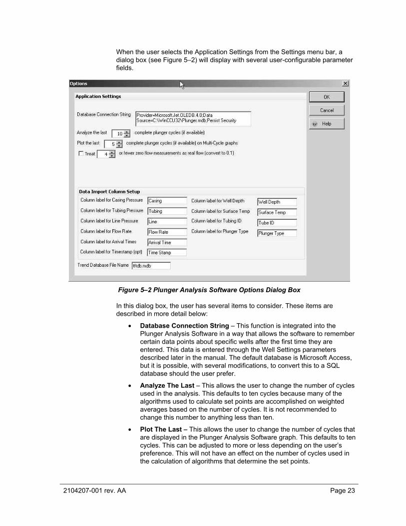
When the user selects the Application Settings from the Settings menu bar, a dialog box (see Figure 5–2) will display with several user-configurable parameter fields.

Figure 5–2 Plunger Analysis Software Options Dialog Box

In this dialog box, the user has several items to consider. These items are described in more detail below:

• Database Connection String – This function is integrated into the Plunger Analysis Software in a way that allows the software to remember certain data points about specific wells after the first time they are entered. This data is entered through the Well Settings parameters described later in the manual. The default database is Microsoft Access, but it is possible, with several modifications, to convert this to a SQL database should the user prefer.

• Analyze The Last – This allows the user to change the number of cycles used in the analysis. This defaults to ten cycles because many of the algorithms used to calculate set points are accomplished on weighted averages based on the number of cycles. It is not recommended to change this number to anything less than ten.

• Plot The Last – This allows the user to change the number of cycles that are displayed in the Plunger Analysis Software graph. This defaults to ten cycles. This can be adjusted to more or less depending on the user’s preference. This will not have an effect on the number of cycles used in the calculation of algorithms that determine the set points.

2104207-001 rev. AA Page 24

• Treat Zero Flows – This setting is available because early testing found several instances in the flow cycle in which the flow reading would become zero for several minutes, while a slug of liquids would completely deplete the flow measurements to zero. This was found on files which had very short log periods sometimes as short as 30 seconds. The default for the checkbox is to be unchecked. This signifies that the function will not be used. When the checkbox is checked, the default is set to four. This is 20 minutes of zero flow (based on the five minute log periods * four periods). If the user has a well that might be shut-in for less than 20 minutes, the user will want to adjust this setting to something less than four. Typically, the user can set this to 1 or 2 unless the user wants to have a well that loads severely, and they notice a trend of not recording the cycles correctly.

• Data Import Column Setup – This section allows the user to set the typical names for the information in the trend file.

It should be noted that if the user chooses to leave the default names within the selected parameters and the Plunger Analysis Software cannot find the appropriate column headings within the corresponding .csv file, the user will receive an error message and be prompted to select the proper column headings from the trend file before the file can be analyzed. This is discussed in more detail later in the manual.

• Trend Database File Name – The default database name is the standard Totalflow naming convention for a unit’s Trend database. If the user is collecting the trend data to another database, they can enter that database name here.

5.2 Importing Data from a .CSV File A basic way to move data into the Plunger Analysis Software is to load the information from a .csv file that was saved onto the user’s computer or a computer on the user’s network.

1) Open the software, and select the trend file from the location where is was initially saved. Typically, when a trend file is collected as a .csv, it will be available in C:\pccu32\spreadsh\archive and then by the trend file name and the meter ID.csv.

2) Using either File > Open .csv File or the Open File icon within the Plunger Analysis Software, navigate to the created trend file that is to be loaded and then open it.

If the trend file that the user is trying to open does not contain the column headings that the Plunger Analysis Software is expecting, the user will receive an Invalid Data File error message. The user is then prompted to configure the column selection by selecting OK.

2104207-001 rev. AA Page 25

3) By clicking the OK button, the user is prompted with another dialog box that has scanned the trend file and compiled a list of column headings. The column headings that match the criteria set in the Application Settings > Data Import Column Setup will be automatically loaded (see Figure 5–3).

4) For columns that are not automatically loaded, select the appropriate column heading from each drop-down list to complete loading the trend file into the Plunger Analysis Software. This feature allows the user to import data from files that may have differing column names.

The available names that are presented in the drop-down list are taken from the collected Trend file. Ensure that the name selected by the user matches the information that the Plunger Analysis Software is looking for.

Figure 5–3 Select Data Columns Dialog Box

5) Click the OK button.

6) Once all of the column names have been identified, if it is the first time a well is being analyzed, a prompt will appear in which the well’s parameters display:

• Tubing ID – Interior Diameters, typical for 2 3/8” tubing is 1.998”

• Surface Temperature – Default is 60°

• Well Depth – This is the depth to which the plunger will stop at the bottom of the tubing

• Plunger Type – Currently, there are three types of plungers available as generic types

7) After these parameters have been configured, click on the Save button.

The application will log these settings to a database that will remember them the next time data from this particular well is loaded into the system. These parameters can be changed by moving to the Settings option on the menu bar and selecting Well Settings from the menu. A dialog box will display where the user

2104207-001 rev. AA Page 26

can modify previous settings in the event new tubing is installed or the type of plunger being used is changed (see Figure 5–4). These new settings will be saved to the well’s name setup and will be the well’s default next time data from the well is loaded into the system.

Figure 5–4 Well Configuration Dialog Box

At the point where the column headings have been identified and the well configuration has been completed, the program will begin formatting the data for display within the Plunger Analysis Software. It can take several seconds for the initial screen to appear which shows the raw trend data. In the view, a well opening is noted by the row highlighted in green, and a well closing is highlighted in red.

Earlier in the manual, settings were made deciding how many cycles would be analyzed and displayed by the Plunger Analysis Software. The number of cycles being analyzed and displayed is also noted at the top left of the grid being displayed. In Figure 5-5, notice the notation: Displaying 10 cycles from trend data and that 18 cycles were actually found (see Figure 5–5).

Figure 5–5 Trend Data Tab

2104207-001 rev. AA Page 27

6.0 VIEWING PLUNGER SETTINGS Once the user has imported a .csv file into the Plunger Analysis Software, they are then given the opportunity to view the plunger settings based on the previously imported .csv file (see Figure 6–1).

Figure 6–1 Plunger Settings Tab

Once the user has moved to the Plunger Settings tab, they are given a variety of sections where they can view the information contained therein.

The parameter fields are auto-populated with the data that was pulled in from the imported .csv file.

The available sections are as follows:

• Well Properties – This section enables the user to view and/or set the well and slug depth. The well properties can be modified through the Settings > Well Settings feature from the menu bar.

• Plunger Fall Times – The Plunger Fall Times section enables the user to see the calculated fall times for the plunger through the tubing including the calculated liquid slug. Additionally, the user can view information on the plunger with or without bypass. Bypass represents a hole through the plunger that, once engaged, will create a void in the plunger and allow it to fall at a greater rate of speed.

• Open When Valve State – The settings displayed in this section enable the user to view the parameters that, once tripped, will cause an Open state. It should be noted that any one of these parameters being engaged will cause the Open state.

2104207-001 rev. AA Page 28

• Plunger Arrival States – The Plunger Arrival Times section enables the user to view the calculated arrive time for the plunger.

• Close When Valve State – The settings displayed in this section enable the user to view the parameters that, once tripped, will cause a Close state. It should be noted that any one of these parameters being engaged will cause a Close state.

• The Turner-Coleman calculations show information regarding the critical rate at which gasses can carry liquid out on its own. If the user selects the checkbox within the section, the user can then modify these parameters based on their specific needs.

7.0 PLUNGER ANALYSIS SOFTWARE TABS The following information will cover the various tabs that the user will encounter within the Plunger Analysis Software.

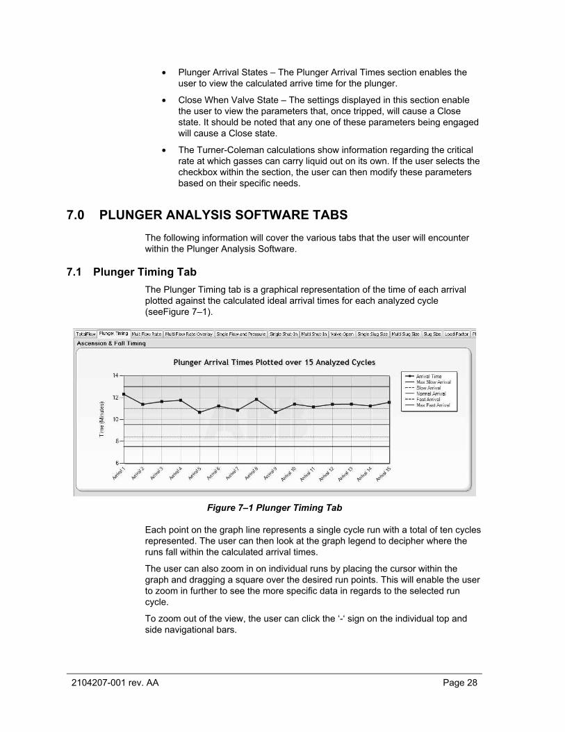
7.1 Plunger Timing Tab The Plunger Timing tab is a graphical representation of the time of each arrival plotted against the calculated ideal arrival times for each analyzed cycle (seeFigure 7–1).

Figure 7–1 Plunger Timing Tab

Each point on the graph line represents a single cycle run with a total of ten cycles represented. The user can then look at the graph legend to decipher where the runs fall within the calculated arrival times.

The user can also zoom in on individual runs by placing the cursor within the graph and dragging a square over the desired run points. This will enable the user to zoom in further to see the more specific data in regards to the selected run cycle.

To zoom out of the view, the user can click the ‘-‘ sign on the individual top and side navigational bars.

2104207-001 rev. AA Page 29

7.2 Multi Flow Rate Tab The Multi Flow Rate tab enables the user to view the flow rate over an extended period of time (see Figure 7–2).

Figure 7–2 Multi Flow Rate Tab

The user can also zoom in on individual points by placing the cursor within the graph and dragging a square over the desired area. This will enable the user to zoom in further to see the more specific data in regards to the selected area.


7.3 Multi Flow Rate Overlay Tab The Multi Flow Rate Overlay tab enables the user to view all of the cycle flow rates overlayed to allow the user to spot patterns and/or outliers (see Figure 7–3).



Additionally, if the user wishes to isolate individual cycle flow rates, they can move the cursor into the graph and right-click. A pop-up menu will display and show each individual cycle run. To temporarily disable individual cycles, click on the checkmark beside the corresponding cycles. The user will then notice that those cycles will disappear out of the graph. By default, all of the cycles are initially turned on.

2104207-001 rev. AA Page 30

Also, within the same pop-up menu, the user is given the option of turning on both the Turner and Coleman parameters. These parameters are critical rate calculations that detail the flow rate that gasses can can carry liquid out of the well on its own. Once turned on, the user will see a red dashed line(s) that show the setpoints for the two individual parameters. The two parameters will also display in the graph legend.

Figure 7–3 Multi Flow Rate Overlay

7.4 Single Flow and Pressure Tab The Single Flow and Pressure tab enables the user to view if the well is running. Additionally, the graph gives a view of how pressures react when the well is open and flowing (see Figure 7–4).

Figure 7–4 Single Flow and Pressure Tab

2104207-001 rev. AA Page 31



Each cycle is shown individually. The user can click the Previous Cycle or Next Cycle buttons at the bottom to navigate to the desired cycle that they want to view.

Additionally, if the user wants to isolate individual cycle flow rates, they can move the cursor into the graph and right-click. A pop-up menu will display and show each individual component. To temporarily disable individual components, click on the checkmark beside the corresponding items. The user will then notice that those items will disappear out of the graph. By default, all of the components are initially turned on.

Also, within the same pop-up menu, the user is given the option of turning on both the Turner Critical Rate and Coleman Critical Rate parameters. These parameters are critical rate calculations that detail the flow rate that gasses can can carry liquid out of the well on its own. Once turned on, the user will see the a red dashed line(s) that show the setpoints for the two individual parameters. The two parameters will also display in the graph legend.

7.5 Single Shut-In Tab The Single Shut-In tab enables the user to view the pressures when the well is shut-in and how the pressure recovers for each individual cycle (see Figure 7–5).




Figure 7–5 Single Shut-In Tab

2104207-001 rev. AA Page 32


Also, within the same pop-up menu, the user is given the option of turning on the Foss and Gaul parameter. This parameters represents the calculation that is used to determine when to open a well based on pressure. Once turned on, the user will see an orange line that represents the Foss and Gaul setting. The parameter will also display in the graph legend.

7.6 Multi Shut-In Tab The Multi Shut-In tab enables the user to view a time slice of how the pressures are reacting from valve open to valve close (see Figure 7–6).




Figure 7–6 Multi Shut-In Tab

2104207-001 rev. AA Page 33

7.7 Valve Open Tab The Valve Open tab shows the user a plot of the pressures that were taken when the valve is preparing to open. Additionally, it uses a linear forecast to estimate the next five open pressures. Of special note to the user is the casing pressure incline or decline (see Figure 7–7).

Figure 7–7 Valve Open Tab



Additionally, if the user wishes to isolate individual information components, they can move the cursor into the graph and right-click. A pop-up menu will display and show each individual component. To temporarily disable individual components, click on the checkmark beside the corresponding items. The user will then notice that those items will disappear out of the graph. By default, all of the components are initially turned on.

7.8 Single Slug Size Tab The Single Slug Size tab gives the user a visual representation of the in-flow and out-flow of fluids when the well is in a shut-in state. This visual representation is presented in feet and gallons of water (see Figure 7–8).




2104207-001 rev. AA Page 34

Figure 7–8 Single Slug Size Tab

7.9 Multi Slug Size Tab The Multi Slug Size Tab gives an overlay of all ten cycles that give the user a visual representation of the in-flow and out-flow of liquids when the well is in a shut-in state (see Figure 7–9).



Figure 7–9 Multi Slug Size Tab

2104207-001 rev. AA Page 35

Additionally, if the user wishes to isolate individual information components, they can move the cursor into the graph and right-click. A pop-up menu will display and show each individual component. To temporarily disable individual components, click on the checkmark beside the corresponding items. The user will then notice that those items will disappear out of the graph. By default, all of the components are initially turned on.

7.10 Slug Size Tab The Slug Size tab shows an individual representation of the fluid level, per run, in feet, barrels and gallons. By clicking on each individual cycle, the user will notice that the Fluid Level (Before Valve Open) section will change to reflect the information for the selected cycle (see Figure 7–10).

Figure 7–10 Slug Size Tab

7.11 Load Factor Tab The Load Factor tab gives the user a view of the plots of the last ten load ratios at the valve opening condition. This serves as an indicator of the well’s ability to lift liquids. The load ratio calculation is represented as casing – tubing/casing – line. Less than .5 or 50% is considered satisfactory. Greater than these numbers, however, is considered unsatisfactory (see Figure 7–11).

2104207-001 rev. AA Page 36

Figure 7–11 Load Factor Tabs



Totalflow Plunger Analysis Software - ABB · PDF file1.2 Plunger Analysis Software Background...

Documents

Transcript of Totalflow Plunger Analysis Software - ABB · PDF file1.2 Plunger Analysis Software Background...