PNA

SPL

US

PHYS

ICS

Topological phenomena in classical optical networksT. Shia,1, H. J. Kimbleb,1, and J. I. Ciraca

aMax-Planck-Institut fur Quantenoptik, 85748 Garching, Germany; and bNorman Bridge Laboratory of Physics, California Institute of Technology,Pasadena, CA 91125

Contributed by H. J. Kimble, September 13, 2017 (sent for review June 5, 2017; reviewed by Mohammad Hafezi and Mikael C. Rechtsman)

We propose a scheme to realize a topological insulator withoptical-passive elements and analyze the effects of Kerr nonlin-earities in its topological behavior. In the linear regime, our designgives rise to an optical spectrum with topological features andwhere the bandwidths and bandgaps are dramatically broadened.The resulting edge modes cover a very wide frequency range.We relate this behavior to the fact that the effective Hamiltoniandescribing the system’s amplitudes is long range. We also developa method to analyze the scheme in the presence of a Kerr medium.We assess robustness and stability of the topological features andpredict the presence of chiral squeezed fluctuations at the edgesin some parameter regimes.

topology | nonlinear | network | optical

The discovery of topological insulators (TIs), as well as quan-tum spin Hall (QSH) insulators (1–9), has opened up a wide

range of scientific and technological questions. Their spectra fea-ture a set of bands, connected by chiral edge modes that reflectthe topological nature of the material. These modes are robustagainst perturbations whose energy does not exceed the corre-sponding bandgap and that do not break the time-reversal (TR)symmetry (10, 11). Electronic interactions give rise to a widerange of phenomena. Although the edge modes persist, theirproperties are qualitatively modified (12). In addition, they cangive rise to other exotic phenomena, like the fractionalization ofcharges, or the appearance of excitations with fractional statistics(13, 14).

Recent proposals to generate TIs and QSH insulators withlight have also attracted a lot of attention (2, 15–27, 28). In fact,the first experimental observations (15, 16) of topological fea-tures in optical systems have been recently reported, and sev-eral schemes exhibiting intriguing features have been proposed(17–25). There exist different setups where one can realize theoptical analog of QSH insulators and observe similar features.In the context of coupled resonator arrays, one can use eitherdifferential optical paths in waveguides (26) or an optical activeelement (27). Despite their success, in the first case it wouldbe desirable to enlarge the bandgaps in the spectrum, which islimited by the small coupling of the local modes in the (high-finesse) resonators (26), to gain robustness. To enlarge the band-width and bandgaps, recently, several proposals in the Floquetsystems (29), microwave networks (30), and strongly coupledspoof-plasmon systems (31) have been studied. In the secondone, photon absorption in the active media also limits the oper-ationality of the scheme. In other schemes, like the one basedon bianisotropic metacrystals (28), the realization of long-livededge modes in a broader frequency range is challenged by theweak bianisotropy in metamaterials (32, 33). To enhance thebianisotropy, an alternative realization has been proposed formetallodielectric photonic crystals in the microwave regime (34).The effects of interactions, including the stability of edge modes,edge solitons, and the quantum dynamics, in those optical mod-els have been also investigated recently (24, 35–42).

In this work we propose and analyze a scheme to realize theoptical version of the QSH insulator and investigate the effectsproduced by Kerr nonlinearities. Our scheme uses beam splittersand birefringent materials that are optically passive and thus cir-cumvent the problem of photon absorption. Our scheme features

several distinct phenomena compared with some of the previousproposals.

In the linear regime, the Hamiltonian description of our setupfeatures long-range hopping, which leads to a dramatic increaseof the spectral bands and bandgaps. This results in a more robustbehavior of the edge modes against perturbations. We analyzequantitatively the robustness of our scheme against losses andcompare it to other models not displaying long-range Hamilto-nian descriptions, as well as to recent experiments (15).

In the nonlinear regime, we obtain the following results: (i) Ina closed network, an arbitrarily small Kerr interaction inducesinstability, a phenomenon we explain in terms of a simple model.(ii) Opening the network and driving it in the appropriate regimestabilizes the system. By tuning the frequency of the driven light,stable bulk and edge modes are both generated. (iii) The smallexcitations around the edge modes are themselves chiral andthus protected. (iv) The edge modes, apart from being chiral, aresqueezed.

In this paper we also introduce theoretical frameworks basedon the S-matrix approach to describe our model both for thelinear and for the nonlinear regimes. The reason why standardapproaches do not apply in the linear regime is that the energyspectrum spreads over the whole free spectral range (FSR), sothat the energy bands in two adjacent ranges connect to eachother. Thus, one cannot use an effective Hamiltonian descrip-tion in each FSR. Furthermore, since the energy spectrum is notlower bounded, the nonlinear behavior is very different from thatof lower-bounded Hamiltonians. The analysis of such behaviorcannot be carried out with standard Bogoliugov techniques, butrequires a sophisticated method based on a nonlinear S-matrixformalism.

Model SetupIn this section, we construct (non)linear classical optical net-works that exhibit nontrivial phenomena. The light propagation

Significance

We introduce a unique scheme to investigate topologicalbehavior, using optical-passive elements and Kerr nonlinear-ities. Compared with previous proposals, the topological bandgaps are dramatically broadened, leading to very robust edgemodes. Our setup displays intriguing phenomena in the non-linear regime, including instabilities and the production ofsqueezed light in the edge modes. This proposal promisesunique avenues for engineering phases of light with topolog-ical character.

Author contributions: T.S., H.J.K., and J.I.C. designed research; T.S., H.J.K., and J.I.C. per-formed research; T.S. contributed new reagents/analytic tools; T.S. analyzed data; andT.S., H.J.K., and J.I.C. wrote the paper.

Reviewers: M.H., University of Maryland; and M.C.R., Pennsylvania State University.

The authors declare no conflict of interest.

This open access article is distributed under Creative Commons Attribution-NonCommercial-NoDerivatives License 4.0 (CC BY-NC-ND).

1To whom correspondence may be addressed. Email: tshi@mpq.mpg.de or hjkimble@caltech.edu.

This article contains supporting information online at www.pnas.org/lookup/suppl/doi:10.1073/pnas.1708944114/-/DCSupplemental.

www.pnas.org/cgi/doi/10.1073/pnas.1708944114 PNAS | Published online October 10, 2017 | E8967–E8976

Dow

nloa

ded

by g

uest

on

Mar

ch 3

0, 2

020

in the nodes and (non)linear fibers is investigated in Nodes andLight Propagation in Fibers, respectively. In Full Networks, weanalyze the boundary conditions for the closed and open net-works in the torus, cylinder, and open plane.

We consider a toy model, i.e., a network of size Nx ×Ny withoptically passive elements. As shown in Fig. 1 A and B, at eachnode of a square lattice, two beamsplitters and two perfect mir-rors form a “bad cavity” to change the propagation direction ofincoming light in the optical fibers with length L. The fibers 1 and4 are connected to the beamsplitter A, and the fibers 2 and 3 areconnected to the beamsplitter B .

Since the polarizations of light are always orthogonal to thepropagation direction, the directions of vertical polarization Vin the horizontal and vertical fibers are different. As shown inFig. 1B, the directions of horizontal polarization H are chosen tobe pointing out of the 2D plane, while the directions of verticalpolarization V are pointing up and right in the horizontal andvertical fibers, respectively.

Nodes. In this subsection we study the light propagation in thenode, where the relation of input and output amplitudes Ψa =

(ar , au , al , ad)T and Ψb = (br , bu , bl , bd)T (Fig. 1B) is estab-lished by the scattering matrix (S matrix) of the node. Here,the two-component amplitudes ar,u,l,d and br,u,l,d are defined inthe linear polarization basis (H ,V ). As shown in Fig. 1B, in theinner cavity, the input and output amplitudes of the beamsplit-

1

2

3

y

1 2 3

X nM

x

L

rada

la

ua

lb

rb

ub

db

ucrclc

dc VH

VH

A

BC

DE

F

Kerr medium

,r nmb ,r nmb ,r nma

,u nma

,u nmb

Kerr m

edium

X nM

Node

1

2

3

4A B

C D

Fig. 1. Scheme of our optical network. (A) The planar network. (B) A nodeconnects horizontal and vertical links. Here, ar, u, l, d and br, u, l, d denote theinput and output amplitudes, and cr, u, l, d denotes the amplitudes in thecavity. The horizontal and vertical polarizations (H,V) in fibers are shownby the red circles and arrows. (C) The horizontal and vertical links with theKerr medium and birefringent elements, where the Kerr medium is put onthe right-hand side of three birefringent elements in the horizontal link,where the birefringent elements are assumed to have no Kerr nonlinear-ity (χ= 0). From left to right, the three birefringent elements are describedby the Jones matrices X = eiπσx/4, Mn = einθ0σz , and X† in the linear polar-ization basis (H, V). (D) The σ+ polarized light acquires the phase θ0 (−θ0)by propagating (anti)clockwisely in each plaquette, while the σ− polarizedlight acquires the phase −θ0 (θ0) by propagating (anti)clockwisely in eachplaquette.

ter A are cu,l and cr,d , and the elements C and D are perfectlyreflecting mirrors.

The relation

S(A)bs

σzarcuclad

=

crbuσzblcd

;S(B)bs

cdσzaualcr

=

brclcuσzbd

, [1]

between amplitudes ar,u,l,d , br,u,l,d , and cr,u,l,d is determined bythe S -matrix S

(A)bs =S

(B)bs ≡Sbs,

Sbs =

tbs irbsσz 0 0irbsσz tbs 0 0

0 0 tbs irbsσz

0 0 irbsσz tbs

[2]

of beamsplitters A and B , where the real reflection and trans-mission coefficients are rbs and tbs =

√1− r2

bs. In Eq. 1, wehave assumed that the size of the node is much smaller than thewavelength of light such that the free propagation phase in thenode can be neglected. In principle, for a node cavity of smalldimensions compared with the optical wavelength, the diffrac-tion effect should be considered and a full finite-difference time-domain method might be required. In practice, one should con-sider designing coupling directly the fiber to the cavities and adesign such that losses are negligible. Under such conditions,the node will be characterized by a set of parameters, i.e., thereflection and transmission coefficients, that could be adjustedto match the toy model considered here. We expect that our toymodel can capture the main physics in the system. A similar treat-ment was used in ref. 27.

Due to the Fresnel reflection rule, for the incoming verticalpolarized light from the fiber 1 (3), the reflecting light in the fiber4 (2) changes the sign. The sign change for the vertical polariza-tion is described by the Pauli matrix σz in Eq. 2. To cancel thisFresnel effect, two birefringent elements E and F in close prox-imity to the beamsplitters (A,B) in the fibers 1 and 2 have beenintroduced and are described by the Jones matrix σz in Eq. 1.

Eliminating the inner-cavity fields cr,u,l,d , we derive the scat-tering equation SnodeΨa = Ψb at the node, where the S -matrix

Snode =

0 irnode 0 tnode

irnode 0 tnode 00 tnode 0 irnode

tnode 0 irnode 0

[3]

relates the input and the output amplitudes Ψa and Ψb . At thenode, the effective reflection and transmission coefficients arernode = 2rbs/(1 + r2

bs) and tnode = t2bs/(1 + r2

bs), respectively. Inour scheme, we choose rbs =

√2− 1, such that rnode = tnode =

1/√

2 maximizes the topological bandwidth and bandgap definedlater on.

Light Propagation in Fibers. In this subsection, we use a waveequation to study the light propagation in the nonlinear fiberconnecting two adjacent nodes, where the birefringent elementsare introduced to induce the artificial gauge field for the light. Bysolving the wave equation, we obtain the input–output relation ofthe amplitudes at adjacent nodes.

Fig. 1C shows that in each horizontal fiber, three birefrin-gent elements described by the Jones matrices X = e iπσx/4,Mn = e inθ0σz , and X † are placed close to the node on the leftside of the horizontal fiber, where σx ,y,z are Pauli matrices in thepolarization basis (H ,V ). The element with the row-dependentJones matrix Mn generates the opposite phase shifts ±nθ0 forthe H - and V -polarized light, and the element with the Jonesmatrix X induces the phase shifts ±π/4 for the linear polar-ized light (H ±V )/

√2. The birefringent elements cause the

light to acquire a phase matrix θ0σy by propagating around

E8968 | www.pnas.org/cgi/doi/10.1073/pnas.1708944114 Shi et al.

Dow

nloa

ded

by g

uest

on

Mar

ch 3

0, 2

020

PNA

SPL

US

PHYS

ICS

each plaquette. Eventually, circular polarizations (H ± iV )/√

2(σ±) experience oppositely directed “magnetic” fields with fluxes±θ0 (Fig. 1D), which induces a nontrivial Z2 topology in thisTR-invariant system.

The interaction of light in the fiber, induced by a Kerr non-linearity (Fig. 1C), leads to the additional phase proportional tothe light intensity. We set to zero the cross-phase modulationbetween orthogonal circular polarizations in the Kerr nonlinear-ity, as discussed in ref. 43, chap. 6 and ref. 44, chap. 4. As a result,the two polarizations are decoupled, and we are able to treat theσ± polarizations independently, as long as these polarizationsare separately excited by the external input (i.e., only σ+ or σ−polarization circulating in the fiber links).

In the Kerr medium of the fiber connecting nodes (n,m) and(n,m − 1), the right- and left-moving fields φr(l),nm (denotingthe left or right polarized light) obey the motion equations (45–47) (we use the matrix convention (n,m) to label the sites, wheren is the row index and m is the column index; we note that thematrix convention is different from the coordinate convention(x , y) that labels the row and column by y and x , respectively)

i∂tφr,nm(x , t) + i∂xφr,nm(x , t)

= χ[|φr,nm(x , t)|2 + 2|φl,nm−1(x , t)|2]φr,nm(x , t), [4]

and

i∂tφl,nm−1(x , t)− i∂xφl,nm−1(x , t)

= χ[|φl,nm−1(x , t)|2 + 2|φr,nm(x , t)|2]φl,nm−1(x , t), [5]

where x is the distance along the fiber and χ describes the self-focusing Kerr interaction (43, 48). In Light Propagation in Single-Segment Nonlinear Fiber and Figs. S1 and S2, we give the solutionof the motion Eqs. 4 and 5 in detail.

The wave Eq. 4 has the solution

φ(0)r,nm(x , t) = ar,nme ikr (x−L)e−iωt ,

φ(0)l,nm−1(x , t) = al,nm−1e

−iklxe−iωt , [6]

where, as shown in Fig. 1C, ar,nm is the amplitude of the right-moving input field to the node (n,m), and al,nm−1 is the ampli-tude of the left-moving input field to the birefringent elements.The wave vectors

kr = ω − χ[|ar,nm |2 + 2|al,nm−1|2],

kl = ω − χ[|al,nm−1|2 + 2|ar,nm |2] [7]

of the right- and left-moving fields are determined by the inten-sities of the fields and the frequency ω of light in the fiber.

The solution 6 results in the relation

e−inσθ0br,nm = br,nm = e−ikrLar,nm ,

e inσθ0bl,nm−1 = e−iklLe inσθ0 al,nm−1 = e−iklLal,nm−1, [8]

where br,nm is the amplitude of the right-moving output field outof the node (n,m−1), br,nm is the amplitude of the right-movingfield on the right-hand side of the birefringent elements, bl,nm−1

is the amplitude of the left-moving output field out of the node(n,m), al,nm−1 is the amplitude of the left-moving input field tothe node (n,m − 1), and σ = ±1 for the two orthogonal circularpolarizations.

The same analysis is applied to the light propagation in thevertical fiber connecting the nodes (n,m) and (n + 1,m). Thesteady-state solution of Eq. 5 results in the relation

bu,nm = e−ikuLau,nm , bd,n+1m = e−ikdLad,n+1m , [9]

for the amplitudes of input fields au,nm , ad,n+1m and outputfields bu,nm , bd,n+1m (as shown in Fig. 1C), where the wave vec-tors are

ku = ω − χ[|au,nm |2 + 2|ad,n+1m |2],

kd = ω − χ[|ad,n+1m |2 + 2|au,nm |2]. [10]

The S -matrix 3 of the node and the relations 8 and 9 determinethe light distribution in the bulk of the network.

Full Networks. In this subsection, different boundary conditionsare studied for the closed networks in the torus, cylinder, andopen plane. To generate the nontrivial topological states in thenetwork, we drive the open network by external light through theboundary.

To realize the cylindrical and planar geometries, perfect mir-rors are placed along the boundaries to form the closed network,where the distance between the boundary mirror and the bound-ary node is L/2 (Fig. 2 A and B). The boundary conditions are

ar,nNx+1 = ar,n1, al,n0 = al,nNx ,

au,0m = au,Nym , ad,Ny+1m = ad,1m [11]

for the network in the torus,

ar,nNx+1 = ar,n1, al,n0 = al,nNx ,

au,0m = ad,1m , ad,Ny+1m = au,Nym [12]

for the closed cylindrical network with the periodic boundarycondition along the x direction, and

ar,nNx+1 = al,nNx , al,n0 = ar,n1,

au,0m = ad,1m , ad,Ny+1m = au,Nym [13]

for the planar network with boundary perfect mirrors.Through the partially transmissive mirrors at the boundary of

the open networks, nontrivial topological states can be gener-ated by the external optical driving field. For the open cylindricalnetwork, we drive the network through the top boundary mir-rors with the reflection (transmission) coefficient rBM (tBM), asshown in Fig. 2C, where the driving light of frequency ωd has theamplitude A

(0)in,m . The corresponding boundary condition

2L

y

x

Network

2L

x

y

,in mA ,out mA

,1d ma ,0u mb

boundary mirrors

m

inA,11ra

RA,10lb

, x yl N Na

TA

boundary mirror

boundary mirror

Network

A B

C D

Fig. 2. Scheme for the boundary mirrors in the cylindrical and planar net-works. (A and B) Perfect and partially transmissive mirrors are put along theboundaries of the cylindrical (A) and planar (B) networks. Here, the partiallytransmissive mirrors are placed along the top boundary in the cylindricalnetwork and at the top left and bottom right corners in the planar network.The driving light (red arrows) is applied to generate the excitations and thetransmitted light (blue arrow). (C) Driven cylindrical network through eachof the partially transmissive mirrors on the top boundary. (D) Light reflec-tion and transmission through the boundary mirrors next to the nodes (1, 1)and (Ny , Nx) in the planar network (i.e., nodes in the top left and bottomright corners of the planar network).

Shi et al. PNAS | Published online October 10, 2017 | E8969

Dow

nloa

ded

by g

uest

on

Mar

ch 3

0, 2

020

SBM

(A

(0)in,m

bu,0me iωdL/2

)=

(ad,1me−iωdL/2

A(0)out,m

)[14]

is determined by the S -matrix

SBM =

(tBM irBM

irBM tBM

)[15]

of the transmissive mirrors, where A(0)out,m is the amplitude of the

output field above the boundary mirror (Fig. 2C), and ad,1m andbu,0m are the amplitudes of the down-moving input field and theup-moving output field at the top of the cylinder [i.e., the bound-ary node (1,m)].

For the open planar network, we drive the network throughthe partially transmissive mirror next to the node (1, 1) withlight of frequency ωd and detect the transmission to the node(Nx ,Ny), as shown in Fig. 2D. The boundary condition is

SBM

(A

(0)in

bl,10eiωdL/2

)=

(ar,11e

−iωdL/2

AR

),

SBM

(br,NyNx+1e

iωdL/2

0

)=

(AT

al,NyNx e−iωdL/2

), [16]

where A(0)in denotes the input amplitude to the network, and AR

(AT) is the reflection (transmission) amplitude. The amplitudesof right-moving input and left-moving output fields at the node(1, 1) are ar,11 and bl,10, while the amplitudes of left-movinginput and right-moving output fields at the node (Nx ,Ny) areal,NyNx and br,NyNx+1.

Using the S -matrix 3 at the node, the relations 8 and 9, and theboundary conditions 14 and 16, we can establish the scatteringequations for the entire network in the different geometries. Thedetails are shown in Scattering Equations on Different Geometries.

Linear RegimeIn this section, we use the scattering equation to study thetopological phenomena in the linear network without the Kerrmedium. In Topological Band Structures in Closed Networks, westudy the photonic spectra E by solving the scattering equationfor the closed networks in the torus, cylinder, and open plane.We find that the edge states appear in the bandgaps coveringa very wide frequency range. In Probe Edge and Bulk Modesin Open Networks, we show that the edge and bulk modes canbe generated by the external driving light and detected by thespectroscopic analysis of the transmitted light. The robustness ofthe edge modes against losses and imperfections is analyzed inRobustness of the Edge Modes in Open Networks.

The photonic spectra E of the closed linear networks in differ-ent geometries exhibit nontrivial topological phenomena, whichare described by the scattering equation. For the bulk degrees offreedoms, the scattering equation

S0

ar,nmau,nmal,nmad,nm

= e−iEL

ar,nm+1

au,n−1m

al,nm−1

ad,n+1m

[17]

follows from Eqs. 8 and 9, where the free S -matrix

S0 =1√2

0 ie−inσθ0 0 e−inσθ0

i 0 1 00 e inσθ0 0 ie inσθ0

1 0 i 0

[18]

connects the right-, up-, left-, and down-moving input fieldsar,u,l,d,nm at the node (n,m) with the input amplitudes ar,nm+1,au,n−1,m , al,nm−1, and ad,n+1m at the four nearest-neighbornodes. We note that the eigenstates of S0 have well-definedpolarization σ+ or σ−.

Topological Band Structures in Closed Networks. Incorporating theboundary conditions 11 and 12 to the scattering Eq. 17, we deter-mine the eigenstates and the corresponding spectrum. Due to thetranslational symmetry, the eigenstate

a(r,u,l,d),nm =1√Nx

a(r,u,l,d),neikxm [19]

has well-defined quasi-momenta kx = −π+2πn/Nx , where n =0, 1, 2, ...,Nx − 1.

Fig. 3 A and B shows the spectra of the networks in the torusand cylinder in the FSR E ∈ωc + (−π/L, π/L] around a largecentral frequency ωc = 2πNc/L, where Nc is a positive integer,and θ0 = π/2.

As shown in Fig. 3A, in the torus the photonic bands spreadover the whole FSR 2π/L and display large bandgaps. Forinstance, for L= 50 µm (15), the FSR is ∼1THz . In contrastto the standard narrow-band schemes (26, 27), the wide-bandspectrum results from the large hopping strength (compara-ble with 2π/L) between nodes beyond nearest neighbors in thebad cavity regime, Rbs = |rbs|2∼ 0.17. In each FSR, this long-range hopping behavior is characterized by the spatially non-local Hamiltonian Heff = i lnS0/L rather than the Hofstadter(tight binding) model (49). Here, we emphasize that even thoughthe S matrix contains only the nearest-neighbor couplings, theeffective Hamiltonian could show long-range hopping behaviorbetween cavity modes since it is determined by the logarithmof the S matrix. One can introduce the creation (annihilation)operators Ck,α of the eigenmodes in the band α to express theeffective Hamiltonian as Heff =

∑k εk,αC

†k,αCk,α, where εk,α

denotes the dispersion relation in the band α.As a consequence of time-reversal symmetry [as in the case

of Z2-protected topological insulators (10)], helical edge modesarise at the broad topological bandgaps. In Fig. 3B, for the cylin-drical geometry, the spectrum displays four edge modes between

A B

C D

Fig. 3. The energy spectra in the torus and cylinder, where θ0 = π/2,the network size is 48 × 48, and L is taken as a unit. Here, we use T±and B± to denote the σ± polarizations on the top and bottom boundaries,respectively. (A and B) The energy spectrum E in the torus (A) and cylinder(B) without phase randomness and losses of linear elements, where B andT denote the bottom and top boundaries, respectively. (C and D) The realpart of the energy spectrum in the torus (C) and cylinder (D) with phaserandomness and nonzero losses of linear elements.

E8970 | www.pnas.org/cgi/doi/10.1073/pnas.1708944114 Shi et al.

Dow

nloa

ded

by g

uest

on

Mar

ch 3

0, 2

020

PNA

SPL

US

PHYS

ICS

the bandgaps, where the chiralities of two edge modes on eachboundary are locked to the σ± polarizations. We focus on theright polarized mode. The Chern number associated to the rightpolarized mode in each subband can be properly defined. Thelowest and highest subbands in each FSR have Chern number1. From the second to the eighth subbands, the Chern num-ber changes alternatively between two values, ±2. As a result,the right polarized edge mode localized at the top boundaryof the cylinder changes its chirality alternatively in differentmidgaps. This band structure is similar to that found in Floquetsystems (50).

These helical edge modes are robust to local perturbationsthat do not break the time-reversal symmetry, as long as thebandgap remains open. As we shall see in Robustness of the EdgeModes in Open Networks, the effects of randomness and lossesare strongly suppressed due to the broadness of the spectrumas a consequence of the low finesse of the cavities. Fig. 3 Cand D shows that for random phase fluctuations δp ∈ [−0.2, 0.2]around θ0 =π/2 and a 10% optical loss in each element, thebandgaps in the energy spectrum ReE are still open in the torus,and the helical edge modes survive in the cylinder with lifetimeτ = 1/ImE ∼ 13L. The losses are described by the nonunitary Smatrix of the optical element.

Probe Edge and Bulk Modes in Open Networks. To generate anddetect the edge and bulk modes, we consider the open networksin the torus and cylinder driven by an external light, as shown inFig. 2 C and D.

For the cylindrical network (Fig. 2A), the input light

A(0)in,m(t) =

1√Nx

A(0)in e ikxm−iωdt [20]

with amplitude A(0)in and frequency ωd is applied through the

transmissive top-boundary mirror. Due to the translational sym-metry in the driven network, the steady-state solution has theform 19. The boundary condition 14 and the scattering Eq. 17result in

SBM

(A

(0)in

bu,0eiωdL/2

)=

(ad,1e

−iωdL/2

A(0)out

), [21]

and

RBMS0(kx )a = e−iωdLa− tBMe−iωdL/2A(0)in [22]

for the field a = (ar,n=1,...,Ny , au,n , al,n ; ad,n)T , where A(0)out is

the amplitude of the output field A(0)out,m = A

(0)oute

ikxm−iωdt/√Nx , RBM is obtained by replacing the diagonal matrix ele-

ment I3Ny+1,3Ny+1 of the 4Ny -dimensional identity matrix I withirBM,

S0(kx ) =1√2

0 ie−ikx e−inσθ0 0 e−ikx e−inσθ0

i 0 1 00 e ikx e inσθ0 0 ie ikx e inσθ0

1 0 i 0

, [23]

and A(0)in =A

(0)in (0; 0; 0; 1)T is composed of the Ny -dimensional

null vector 0 and 1 = (1, 0, ..., 0).The solution of the scattering Eq. 22 determines the output

amplitude

A(0)out =

tBM

irBMe−iωdL/2ad,1 −

A(0)in

irBM. [24]

When the driving frequency ωd is resonant with an eigenfre-quency of the closed system, the boundary condition 21 gives theamplitude

ad,1 =tBM

1− irBMA

(0)in e iωdL/2, [25]

and the input–output relation A(0)out = e iδ0A

(0)in , where the

phase shift

δ0 = arg(

1 + irBM

1− irBM

). [26]

Remarkably, the relative phase δ0−(π+2 arctan rBM)∈ (−π, π]jumps from−π to π when ωd sweeps across a resonant frequencyof the closed network. Thus, the measurement of this phase shiftreveals the spectrum. As shown in Fig. 4A, for σ+ polarized driv-ing light, the peaks of dδ0/dωd show the band structure and thechiral edge mode on the top boundary. The spatial separation ofthe bottom edge mode and the driving light makes the first invis-ible in Fig. 4A, which isolates a single σ+ polarized chiral edgemode on the top boundary.

For the planar network, circularly polarized driving light withamplitude A

(0)in and frequency ωd is injected through the trans-

missive mirror at the upper left corner (Fig. 1C). The boundarycondition 16 and the scattering equation

RBMS0a = e−iωdLa− tBMe−iωdL/2A(0)in [27]

determine the light distribution a = (ar,nm , au,nm , al,nm , ad,nm)T

in the open network, where RBM is obtained by replac-ing the diagonal matrix elements I1,1 and I3NxNy ,3NxNy ofthe4NxNy -dimensional identity matrix I with irBM, and A(0)

in =

A(0)in (1; 0; 0; 0)T .The solution of the scattering Eq. 27 determines the reflection

and transmission amplitudes

AR =tBM

irBMar,11e

−iωdL/2 − A(0)in

irBM,

AT =tBM

irBMal,NyNx e

−iωdL/2. [28]

As shown in Fig. 4B, the transmission spectrum |AT/A(0)in |

2of

the output light through the mirror at the bottom right corner

A B

C D

Fig. 4. Detection of topological properties, where θ0 =π/2, rBM = 0.9,and L is taken as a unit. (A) For the cylindrical geometry, the contour-plot of dδ0/dωd shows the eigenspectrum for the network of size 48× 48.(B) For the open plane of size 16× 16, the eigenspectrum for the closednetwork and the transmission spectrum. (C) The light intensity of thebulk mode under the σ+-polarized driving light. (D) The light intensities

|a(r, u, l, d)/A(0)in |

2of the edge mode in the network under σ+-polarized driv-

ing light. From the right- (left-) and up- (down-)moving fields shown in theTop (Bottom) row, the chirality of the edge mode can be identified.

Shi et al. PNAS | Published online October 10, 2017 | E8971

Dow

nloa

ded

by g

uest

on

Mar

ch 3

0, 2

020

can be identified with the energy spectrum. For a driv-ing frequency ωd∼ 0.03/L (0.37/L) resonant with the bulk(edge) mode, as shown in Fig. 4C (Fig. 4D), the intensities|a(r,u,l,d),nm/A

(0)in |

2display that the light propagates in the bulk

(along the boundary).

Robustness of the Edge Modes in Open Networks. To analyze therobustness of edge modes, we take into account possible imper-fections in the network, including losses and phase fluctuations ofthe linear elements. The edge modes generated by the externaldriving field are robust, which is the result of the broad topolog-ical bandwidth and bandgap. In Robustness of Broadband Setupsand Figs. S3 and S4, we construct another topological networkwith the tunable spectral width and show that a spectrum spread-ing over the whole FSR has a dramatic effect on the robustness.

To show the differences of our network and that in ref. 15, weuse the same input–output configuration, namely, pumping thenetwork through the node (1, 1) and detecting the transmissionlight at the node (Ny , 1). The loss of each element is chosen tobe 0.1% in the linear optical system. In Fig. 5, the light intensityI =

∑s=r,u,l,d |as,nm |

2 in the steady edge state shows that theedge mode completely circulates around the 16× 16 network.

The short lifetime of the edge modes in the narrow-bandsetup can be overcome in the broadband setup. In the narrow-band setup, each resonator has a high finesse (∼102), such thatthe light reflects many times in the resonator, which induces alarge decay to undesired modes. In the broadband setup, the lowfinesse (∼1) of the resonator results in a short time of the lightin the resonator and the small loss to the undesired modes.

Even though the system is not completely immune to thelosses and imperfections that break the TR symmetry and inducebackscattering that changes the polarization, the imperfectionsare strongly suppressed due to the broad width of the spec-trum. We note that the birefringent element is a linear element,which cannot break the TR symmetry. The TR symmetry break-ing mentioned here amounts to the coupling between two polar-izations with opposite chiralities.

For instance, small phase fluctuations δ and δ′ of birefrin-gent elements, i.e., X = e iσx (π/4+δ) and X †= e−iσx (π/4+δ′), can

/ pI I

in

outFig. 5. The intensity of the steady edge mode in the open planar network,where the intrinsic loss is 0.1%, and Ip is the intensity of the pump field.

induce the coupling between σ+ and σ− polarized light. We con-sider driving the planar network of size 16× 16 through the node(1, 1) with σ+-polarized light and detecting the transmitted lightat the node (16, 1). In Fig. 6, the intensities of σ±-polarized edgemodes are shown for δ,δ′ ∈ [−0.05, 0.05] and δ,δ′ ∈ [−0.1, 0.1].For random phase fluctuations δ,δ′ ∈ [−0.05, 0.05], 1% σ+-polarized clockwise propagating light in the network is scatteredto σ−-polarized anticlockwise propagating light, and 1% σ−-polarized light is detected in the transmitted light. For the largerphase fluctuations δ,δ′ ∈ [−0.1, 0.1], 10% σ+-polarized clockwisepropagating light in the network is scattered to σ−-polarizedanticlockwise propagating light, and 12% σ−-polarized light isdetected in the transmitted light. In real experiments, phase fluc-tuations of linear optical elements can be much smaller than0.05. As a result, in the steady state, 99% σ+-polarized chiralmode may survive at the boundary of the network.

Nonlinear RegimeIn this section, we study how the topological properties predictedin the previous section get modified in the nonlinear regime. Werestrict ourselves to the cylindrical network. By driving the opennetwork from the top boundary, we show in Topological BandStructures in Closed Networks that bulk and edge steady states areboth generated. In Probe Edge and Bulk Modes in Open Networks,we analyze the stability of the steady states by means of a gener-alized Bogoliubov theory, where it turns out that the Bogoliubovedge mode can be detected by the squeezing spectrum of thereflected light.

The nonlinear Kerr medium generates a self-focusing inter-action for χ< 0. Here, we consider separately the σ± polariza-tions and thereby avoid the complexity associated to a Kerr non-linearity for σ± polarizations propagating simultaneously in thefiber links (43, 44). The relations 8 and 9 give rise to the scat-tering equation

S0

ar,nmau,nmal,nmad,nm

= e−iωLe iχNnmL

ar,nm+1

au,n−1m

al,nm−1

ad,n+1m

[29]

for the bulk degrees of freedom, where the 4× 4 intensity-dependent matrix Nnm is defined in Scattering Equations on Dif-ferent Geometries.

The effective Hamiltonian provides an insight into the physicsin the interacting case. By projecting the system on a certainband, the effective Hamiltonian can be interpreted as describingweak interacting bosons in a topological band. At the mean-fieldlevel, we could expect that the steady state is a Bose–Einsteincondensate of light, and the fluctuations are described by Bogoli-ubov modes that give rise to squeezing. In the following, we focuson the steady state and fluctuations in the cylindrical network.

Steady-State Solutions. To generate the interacting bulk and edgesteady states, we consider driving the cylindrical network by anexternal field. Circularly polarized pump-field A

(0)in,me−iωdt with

amplitude A(0)in,m =A

(0)in e ikxm/

√Nx is applied through the top

boundary. Due to the translational symmetry along the x direc-tion, the steady-state solution of Eq. 29 has the form 19.

By numerically solving Eq. 29 with the boundary condition 21,we show the total light intensity Np =

∑n,s=r,u,l,d |as,n |

2 vs. the

driving strength∣∣∣A(0)

in

∣∣∣2 in Fig. 7 A and B for two driving fre-

quencies ω(1)d ∼ 0.22/L (Fig. 7A) and ω(2)

d ∼ 4.5× 10−2/L (Fig.7B), respectively, where kx ∼ 0.26 and the size of the network

is Nx = 24, Ny = 12. The |χ|Np vs. |χ|∣∣∣A(0)

in

∣∣∣2 curves display thatfor the given parameters (kx ,ωd), the driving light with amplitude

E8972 | www.pnas.org/cgi/doi/10.1073/pnas.1708944114 Shi et al.

Dow

nloa

ded

by g

uest

on

Mar

ch 3

0, 2

020

PNA

SPL

US

PHYS

ICS

/ pI I

/ pI I

/ pI I

/ pI I

in

out A B

C DFig. 6. A and C show the intensities I±/Ip of the σ±-polarized light in thenetwork for δ, δ′ ∈ [−0.05, 0.05]; B and D show the intensities I±/Ip of theσ±-polarized light in the network for δ, δ′ ∈ [−0.1, 0.1].

A(0)in generates multiple light intensities in the steady state of

the network. As discussed in Bogoliubov Excitations in Nonlin-ear Optics, large domains of the steady-state solutions in Fig. 7 Aand B are unstable to small perturbations. The qualitative originof these complex stabilities can be traced to the behavior of a sin-gle fiber segment with mirrors (47) (Light Propagation in Single-Segment Nonlinear Fiber and Fig. S2).

For driving frequencies ω(1)d and ω(2)

d , Fig. 7 C and D showsthat distinct light distributions |χ|

∣∣a(r,u,l,d),n

∣∣2 are generatedfor the interacting edge and bulk modes, respectively, where thetotal intensity |χ|Np = 5/L, and rBM = 0.9. We emphasize thatthe topologically protected chiral edge mode survives even inthe nonlinear regime, as illustrated in Fig. 7C, where the chiral-ity can be gathered from the fact that the right-moving intensitydominates.

Bogoliubov Excitations in Nonlinear Optics. The stability of steady-state solutions is analyzed in this subsection. Small fluctuationsaround the driving field A

(0)in,m induce excitations around the

steady state. If excitation is exponentially amplified in the real-time evolution, the steady state is not stable. We develop a gener-alized Bogoliubov theory to analyze the properties of the fluctu-ations and the stability of the steady states. We show that aroundthe stable steady state, chiral Bogoliubov edge excitations aresqueezed and can be detected by the squeezing spectrum of thereflected light.

The additional weak probe light

δAinm(t) =

1√Nx

[δA(+)in e ipxme−iωf t + δA

(−)in e iqxme iωf t ] [30]

with frequency ωf through the top boundary induces the fluctu-ation field δas around the steady-state as and the reflected fluc-tuation field δAout

m (t), where px and qx = 2kx − px are the quasi-momenta along the x direction.

To establish the scattering equation for the fluctuation ampli-tudes δas in the entire network, we first study the propagation offluctuation fields in the fiber. By linearizing the motion in Eqs. 4and 5, we obtain

i∂tδΨH + Σ∂x δΨH = MH δΨH , [31]

and

i∂tδΨV + Σ∂x δΨV = MV δΨV , [32]

which describe the dynamics of Bogoliubov fluctuations

δΨH = (δφr,nm , δφl,nm−1, δφ∗r,nm , δφ

∗l,nm−1)

T,

δΨV = (δφu,nm , δφd,n+1m , δφ∗u,nm , δφ

∗d,n+1m)

T [33]

in the horizontal and vertical fibers, respectively. Here, the matri-ces Σ and MH (V ) are defined in Light Propagation in Single-Segment Nonlinear Fiber.

The solution of linearized Eqs. 31 and 32 has the form

δφs,nm(x , t) =1√Nx

[δψs,n,px (x )e ipxme−iωf t

+ δψs,n,qx (x )e iqxme iωf t ]. [34]

The input and output fluctuation fields at the nodes modulatealong the x direction with the quasi-momenta px and qx , wherethe fluctuation amplitudes are related to the boundary value ofthe wavefunctions ψr,n,px and ψr,n,qx as

δar,n,px = δψr,n,px (L), δal,n,px = e inσθ0δψl,n,px (0),

δbr,n,px = e inσθ0δψr,n,px (0), δbl,n,px = δψl,n,px (L),

δau,n,px = δψu,n,px (L), δad,n+1,px = δψd,n+1,px (0),

δbu,n,px = δψu,n,px (0), δbd,n+1,px = δψd,n+1,px (L). [35]

The scattering Eqs. 31 and 32 result in the relations

PH

e−inσθ0δbr,n,pxe−inσθ0δal,n,pxe inσθ0δb∗r,n,qxe inσθ0δa∗l,n,qx

=

δar,n,pxδbl,n,pxδa∗r,n,qxδb∗l,n,qx

, [36]

and

A B

C D

Fig. 7. Light distributions of the nonlinear system in the cylinder, where thesize is 24 × 12, θ0 = π/2, kx = 0.26, and L is taken as a unit. (A and B) Therelation of the total intensity of (A) edge and (B) bulk modes in the networkwith different reflection indexes rBM and the input intensity of driving lightwith frequencies (A) ω(1)

d = 0.22 and (B) ω(2)d = 4.5 × 10−2. (C and D) The

stable internal intensities of (C) edge and (D) bulk modes for |χ|Np = 5 andrBM = 0.9 (red circles in A and B).

Shi et al. PNAS | Published online October 10, 2017 | E8973

Dow

nloa

ded

by g

uest

on

Mar

ch 3

0, 2

020

PV

δbu,n,pxδad,n+1,px

δb∗u,n,qxδa∗d,n+1,qx

=

δau,n,pxδbd,n+1,px

δa∗u,n,qxδb∗d,n+1,qx

[37]

connecting the boundary values of the fields in the horizontaland vertical fibers, respectively, where the propagation matricesPH (V ) = eΣ(ωf−MH(V ))L and MH (V ) are defined in PropagationMatrices of Bogoliubov Excitations.

Additionally, the boundary values of the fields in adjacentfibers are related by the input–output formula

Sf ,node(px )

δar,n,pxδau,n,pxδal,n,pxδad,n,px

=

e ipx δbr,n,pxδbu,n−1,px

e−ipx δbl,n,pxδbd,n+1,px

[38]

at each node, where

Sf ,node(px ) = e iωdLe−i χ

NxN

nL

e−ipx 0 0 00 1 0 00 0 e ipx 00 0 0 1

Snode.

[39]

The propagation Eqs. 36 and 37 and the input–output relation38 result in the scattering equation for the fluctuation amplitudesin the bulk. To analyze the properties of those fluctuations andthe stability of the steady states, the boundary conditions for thefluctuation fields are required.

The boundary condition

irBMδbu,0,px = e−iωfLδad,1,px − tBMδA(+)in e i(ωd−ωf )

L2 ,

irBMδbu,0,qx = e iωfLδad,1,qx − tBMδA(−)in e i(ωd+ωf )

L2 , [40]

for the fluctuation amplitudes follows from Eq. 21, and the out-put field is

δAoutm (t) =

1√Nx

[δA(+)out e

ipxme−iωf t + δA(−)out e

iqxme iωf t ], [41]

where the components

δA(+)out =

tBM

irBMe−i(ωd+ωf )

L2 δad,1,px −

δA(+)in

irBM,

δA(−)out =

tBM

irBMe−i(ωd−ωf )

L2 δad,1,qx −

δA(−)in

irBM. [42]

Eliminating the output fluctuation fields δbs,n,px (qx ) in Eqs. 36–38 and 40, we establish the linearized scattering equation

D(ωf)

(δapx

δa∗qx

)= tBM

(δA(+)

in e i(ωd−ωf )L2

δA(−)∗in e−i(ωd+ωf )

L2

)[43]

for the fluctuations, where

δapx = (δar,n,px , δau,n,px , δal,n,px , δad,n,px )T , [44]

and δA(±)in = δA

(±)in (0; 0; 0; 1). The steady state is stable if the

fluctuations are not amplified during the time evolution. This sta-ble condition demands that all of the roots Ef of detD(ωf) havenegative imaginary part, i.e., ImEf < 0.

By solving the fluctuation Eq. 43, we mark the stable regimes

by black circles in the χNp vs. χ∣∣∣A(0)

in

∣∣∣2 curves for the steadystates with rBM = 0.9 in Fig. 7 A and B. We find that the steadystates shown in Fig. 7 C and D are in the stable regime.

Eq. 42 and the solution (δapx , δa∗qx ) of Eq. 43 lead to the input–output relation (

δA(+)out

δA(−)∗out

)= MIO

(δA

(+)in

δA(−)∗in

), [45]

where the 2× 2 matrix

MIO =1

irBMσz [t2

BMe−iωfLe−iωdL2σz D(ω)e iωd

L2σz − I2] [46]

is determined by

D(ω) =

([D−1(ω)]3Ny+1,3Ny+1 [D−1(ω)]3Ny+1,7Ny+1

[D−1(ω)]7Ny+1,3Ny+1 [D−1(ω)]7Ny+1,7Ny+1

).

[47]

Induced by the light “condensation” as,n , the Bogoliubov fluc-tuation δas,px ,n couples to the conjugate amplitude δa∗s,qx ,n . Asa result, the probe light with positive frequency, i.e., δA(−)

in = 0,induces a chiral Bogoliubov fluctuation, which eventually gener-ates the squeezed reflected light δAout,m(t). (We emphasize thatour results from the fluctuation analysis for the classical light arealso valid in the quantum regime, where the squeezing behaviorsof quantum edge fluctuations arise from the interplay of the Kerrnonlinearities and topological effects.) The squeezing behavior ischaracterized by the squeezing spectra S+ =

∣∣∣δA(+)out/δA

(+)in

∣∣∣ and

S−=∣∣∣δA(−)

out /δA(+)in

∣∣∣, where the expression S2+ − S2

−= 1 reflectsthe bosonic nature of light.

We note that squeezing of light in topological insulators hasbeen investigated in the context of optical parametric down-conversion systems (24), where the χ(2) nonlinearity is treatedat the mean-field level and quadratic terms with double creation(annihilation) operators are directly introduced in the Hamilto-nian to describe the generation of squeezed light.

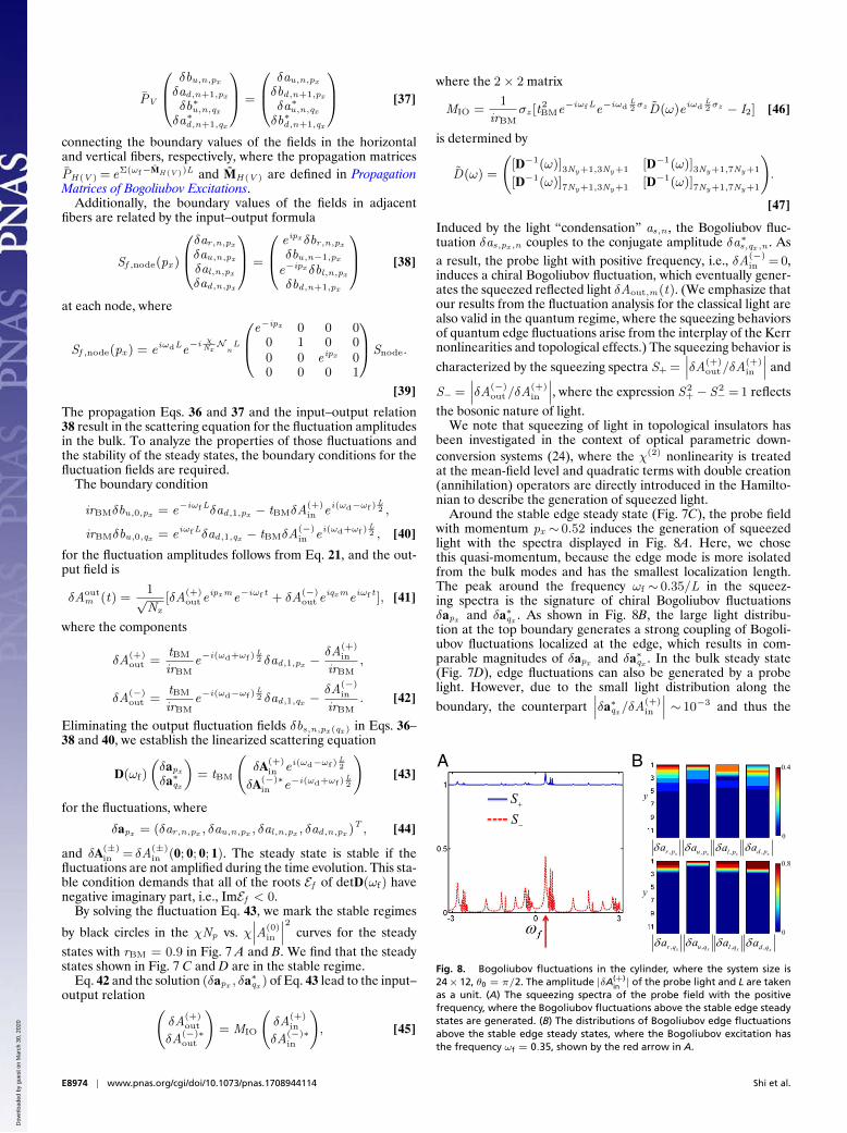
Around the stable edge steady state (Fig. 7C), the probe fieldwith momentum px ∼ 0.52 induces the generation of squeezedlight with the spectra displayed in Fig. 8A. Here, we chosethis quasi-momentum, because the edge mode is more isolatedfrom the bulk modes and has the smallest localization length.The peak around the frequency ωf ∼ 0.35/L in the squeez-ing spectra is the signature of chiral Bogoliubov fluctuationsδapx and δa∗qx . As shown in Fig. 8B, the large light distribu-tion at the top boundary generates a strong coupling of Bogoli-ubov fluctuations localized at the edge, which results in com-parable magnitudes of δapx and δa∗qx . In the bulk steady state(Fig. 7D), edge fluctuations can also be generated by a probelight. However, due to the small light distribution along theboundary, the counterpart

∣∣∣δa∗qx /δA(+)in

∣∣∣ ∼ 10−3 and thus the

A B

Fig. 8. Bogoliubov fluctuations in the cylinder, where the system size is24× 12, θ0 = π/2. The amplitude |δA(+)

in | of the probe light and L are takenas a unit. (A) The squeezing spectra of the probe field with the positivefrequency, where the Bogoliubov fluctuations above the stable edge steadystates are generated. (B) The distributions of Bogoliubov edge fluctuationsabove the stable edge steady states, where the Bogoliubov excitation hasthe frequency ωf = 0.35, shown by the red arrow in A.

E8974 | www.pnas.org/cgi/doi/10.1073/pnas.1708944114 Shi et al.

Dow

nloa

ded

by g

uest

on

Mar

ch 3

0, 2

020

PNA

SPL

US

PHYS

ICS

edge Bogoliubov fluctuations hardly respond to the drivingfield δA(+)

in .In this nonlinear regime our system displays a set of phenom-

ena that are quite different from the results in previous works(51–55): (i) A closed nonlinear network is unstable, and the sys-tem becomes stable by including losses; (ii) around the stableedge steady state, a probe field with a second frequency developssmall edge Bogoliubov fluctuations which turn out to be chiral;(iii) the presence of squeezing, a quantum feature, is identifiedin the edge modes. The reason for the appearance of these phe-nomena is that the energy bands in different FSRs connect toeach other, so that the system cannot be described by a lower-bounded Hamiltonian.

Experimental ParametersIn experimental implementations, one could take a fiber withL= 50 µm and cross section 2× 10−7 cm2, such that the bandsspread over the broad FSR with 1 THz in the linear network.

For the nonlinear network, the relevant parameter is the unit-

less phase ϕ=χ∣∣∣A(0)

in

∣∣∣2L induced by the Kerr interaction. Interms of the experimental parameters, the phase ϕ∼ 2k0n2I0Lis determined by the wavevector k0 in the optical fiber, thesecond-order nonlinear refractive index n2, the intensity I0 =P/A (power/area) of the pump field, and the length of the fiberL, where the optical fiber with k0∼ 4.2× 104 cm−1, and the sec-tion A∼ 2× 10−7 cm2.

For the electronic Kerr effect with small n2∼ 10−16 cm2/W, alength of the link L∼ 10 m of the fiber and a power P = 20 W

of the pump field should be large enough to realize a phaseshift ϕ∼ 1. To realize the large nonlinearity in the small net-work with L∼ 50 µm, one can use the thermal Kerr effect withn2∼ 10−6 cm2/W . A pump power P0 ranging from 4× 10−4 Wto 4× 10−3 W gives rise to nonlinear phase shifts ranging fromϕ= 1∼ 10.

We note that our proposal could also be implemented in theall-in-fiber temporal lattice setup (56).

ConclusionsWe have proposed a scheme to display QSH phenomena usingclassical light and passive optical elements. Compared with pre-vious schemes, ours features broad topological bandgaps. Foropen networks in the linear regime, chiral edge modes appearat the bandgaps and are very robust against losses and randomphase fluctuations. Adding Kerr nonlinearities in the fibers leadsto interacting bulk and edge states that also display topologicalproperties. For closed networks, the system becomes unstable.This can be avoided by opening it. We also predict squeezing inthe chiral edge modes.

ACKNOWLEDGMENTS. This work was funded by the European Union Inte-grated project SIQS. H.J.K. acknowledges support as a Max-Planck Insti-tute for Quantum Optics Distinguished Scholar; as well as funding fromthe Air Force Office of Scientific Research Multidisciplinary UniversityResearch Initiative (MURI) Quantum Many-Body Physics with Photons; theOffice of Naval Research (ONR) Award N00014-16-1-2399; the ONR Quan-tum Opto-Mechanics with Atoms and Nanostructured Diamond (QOMAND)MURI; National Science Foundation (NSF) Grant PHY-1205729; and theInstitute for Quantum Information and Matter, an NSF Physics FrontiersCenter.

1. Thouless DJ, Kohmoto M, Nightingale MP, den Nijs M (1982) Quantized Hall conduc-tance in a two-dimensional periodic potential. Phys Rev Lett 49:405–408.

2. Haldane FDM (1988) Model for a quantum Hall effect without Landau levels:Condensed-matter realization of the “parity anomaly”. Phys Rev Lett 61:2015–2018.

3. Hasan MZ, Kane CL (2010) Colloquium: Topological insulators. Rev Mod Phys 82:3045–3067.

4. Qi X-L, Zhang S-C (2011) Topological insulators and superconductors. Rev Mod Phys83:1057–1110.

5. Kane CL, Mele EJ (2005) Quantum spin Hall effect in graphene. Phys Rev Lett95:226801.

6. Konig M, et al. (2007) Quantum spin Hall insulator state in HgTe quantum wells.Science 318:766–770.

7. Hsieh D, et al. (2008) A topological Dirac insulator in a quantum spin Hall phase.Nature 452:970–974.

8. Zhang H, et al. (2009) Topological insulators in Bi2Se3, Bi2Te3 and Sb2Te3 with asingle Dirac cone on the surface. Nat Phys 5:438–442.

9. Chang CZ, et al. (2013) Experimental observation of the quantum anomalous Halleffect in a magnetic topological insulator. Science 340:167–170.

10. Kane CL, Mele EJ (2005) Z2 topological order and the quantum spin Hall effect. PhysRev Lett 95:146802.

11. Fu L, Kane CL (2006) Time reversal polarization and a Z2 adiabatic spin pump. PhysRev B 74:195312.

12. Wen XG (1992) Theory of the edge states in fractional quantum Hall effects. Int J ModPhys B 6:1711–1762.

13. Laughlin RB (1983) Anomalous quantum Hall effect: An incompressible quantum fluidwith fractionally charged excitations. Phys Rev Lett 50:1395–1398.

14. Moore G, Read N (1991) Nonabelions in the fractional quantum Hall effect. Nucl PhysB 360:362–396.

15. Hafezi M, Mittal S, Fan J, Migdall A, Taylor JM (2013) Imaging topological edge statesin silicon photonics. Nat Photon 7:1001–1005.

16. Rechtsman MC, et al. (2013) Photonic Floquet topological insulators. Nature 496:196–200.

17. Dalibard J, Gerbier J, Juzeliunas F, Ohberg G (2011) Colloquium: Artificial gaugepotentials for neutral atoms. Rev Mod Phys 83:1523–1543.

18. Shi T, Cirac JI (2013) Topological phenomena in trapped-ion systems. Phys Rev A87:013606.

19. Haldane FDM, Raghu S (2008) Possible realization of directional optical waveguidesin photonic crystals with broken time-reversal symmetry. Phys Rev Lett 100:013904.

20. Wang Z, Chong Y, Joannopoulos JD, Soljacic M (2009) Observation of unidirectionalbackscattering-immune topological electromagnetic states. Nature 461:772–775.

21. Fang K, Yu Z, Fan S (2012) Realizing effective magnetic field for photons by control-ling the phase of dynamic modulation. Nat Photon 6:782–787.

22. Yuan L, Fan S (2015) Topologically nontrivial Floquet band structure in a system under-going photonic transitions in the ultrastrong-coupling regime. Phys Rev A 92:053822.

23. Walter S, Marquardt F (2016) Classical dynamical gauge fields in optomechanics. NewJ Phys 18:113029.

24. Peano V, Houde M, Brendel C, Marquardt F, Clerk AA (2016) Topological phase tran-sitions and chiral inelastic transport induced by the squeezing of light. Nat Commun7:10779.

25. Umucalılar RO, Carusotto I (2012) Fractional quantum Hall states of photons in anarray of dissipative coupled cavities. Phys Rev Lett 108:206809.

26. Hafezi M, Demler EA, Lukin MD, Taylor JM (2011) Robust optical delay lines withtopological protection. Nat Phys 7:907–912.

27. Umucalılar RO, Carusotto I (2011) Artificial gauge field for photons in coupled cavityarrays. Phys Rev A 84:043804.

28. Khanikaev AB, et al. (2013) Photonic topological insulators. Nat Mater 12:233–239.

29. Pasek M, Chong Y (2014) Network models of photonic Floquet topological insulators.Phys Rev B 89:075113.

30. Hu W, et al. (2015) Measurement of a topological edge invariant in a microwavenetwork. Phys Rev X 5:011012.

31. Gao F, et al. (2016) Probing topological protection using a designer surface plasmonstructure. Nat Commun 7:11619.

32. Pendry JB, Holden AJ, Stewart WJ, Youngs I (1996) Extremely low frequency plasmonsin metallic mesostructures. Phys Rev Lett 76:4773–4776.

33. Smith DR, Padilla WJ, Vier DC, Nemat-Nasser SC, Schultz S (2000) Composite mediumwith simultaneously negative permeability and permittivity. Phys Rev Lett 84:4184–4187.

34. Cheng X, et al. (2016) Robust reconfigurable electromagnetic pathways within a pho-tonic topological insulator. Nat Mater 15:542–548.

35. Bahat-Treidel O, Segev M (2011) Nonlinear wave dynamics in honeycomb lattices.Phys Rev A 84:021802(R).

36. Bekenstein R, Nemirovsky J, Kaminer I, Segev M (2014) Shape-preserving acceleratingelectromagnetic wave packets in curved space. Phys Rev X 4:011038.

37. Lumer Y, Rechtsman MC, Plotnik Y, Segev M (2016) Instability of bosonictopological edge states in the presence of interactions. Phys Rev A 94:021801(R).

38. Ablowitz MJ, Curtis CW, Ma Y-P (2014) Linear and nonlinear traveling edge waves inoptical honeycomb lattices. Phys Rev A 90:023813.

39. Leykam D, Chong Y (2016) Edge solitons in nonlinear-photonic topological insulators.Phys Rev Lett 117:143901.

40. Rechtsman MC, et al. (2016) Topological protection of photonic path entanglement.Optica 3:925–930.

41. Mittal S, Orre VV, Hafezi M (2016) Topologically robust transport of entangled pho-tons in a 2D photonic system. Opt Express 24:15631–15641.

42. Bardyn C-E, Karzig T, Refael G, Liew TC (2016) Chiral Bogoliubov excitations in non-linear bosonic systems. Phys Rev B 93:020502(R).

43. Agrawal GP (2013) Nonlinear Fiber Optics (Academic, San Diego).44. Boyd RW (2008) Nonlinear Optics (Academic, Rochester, NY).45. Yu M, McKinstrie CJ, Agrawal GP (1998) Temporal modulation instabilities of coun-

terpropagating waves in a finite dispersive Kerr medium. I. Theoretical model andanalysis. J Opt Soc Am B 15:607–616.

Shi et al. PNAS | Published online October 10, 2017 | E8975

Dow

nloa

ded

by g

uest

on

Mar

ch 3

0, 2

020

46. Yu M, McKinstrie CJ, Agrawal GP (1998) Temporal modulation instabilities of counter-propagating waves in a finite dispersive Kerr medium. II. Application to Fabry Perotcavities. J Opt Soc Am B 15:617–624.

47. Firth WJ (1981) Stability of nonlinear Fabry-Perot resonators. Opt Commun 39:343–346.

48. Adair R, Chase LL, Payne SA (1989) Nonlinear refractive index of optical crystals. PhysRev B 39:3337–3350.

49. Hofstadter DR (1976) Energy levels and wave functions of Bloch electrons in rationaland irrational magnetic fields. Phys Rev B 14:2239–2249.

50. Rudner MS, Lindner NH, Berg E, Levin M (2013) Anomalous edge states and the bulk-edge correspondence for periodically driven two-dimensional systems. Phys Rev X3:031005.

51. Carusotto I, Ciuti C (2013) Quantum fluids of light. Rev Mod Phys 85:299–366.

52. Bleu O, Solnyshkov DD, Malpuech G (2016) Interacting quantum fluid in a polaritonchern insulator. Phys Rev B 93:085438.

53. Umucalılar RO, Carusotto I (2012) Fractional quantum Hall states of photons in anarray of dissipative coupled cavities. Phys Rev Lett 108:206809.

54. Lumer Y, Plotnik Y, Rechtsman MC, Segev M (2013) Self-localized states in photonictopological insulators. Phys Rev Lett 111:243905.

55. Barnett R (2013) Edge-state instabilities of bosons in a topological band. Phys Rev A88:063631.

56. Regensburger A, et al. (2012) Parity time synthetic photonic lattices. Nature 488:167–171.

E8976 | www.pnas.org/cgi/doi/10.1073/pnas.1708944114 Shi et al.

Dow

nloa

ded

by g

uest

on

Mar

ch 3

0, 2

020