On the axioms of topological...

Ann. Phys. (Leipzig) 14, No. 6, 347 – 377 (2005) / DOI 10.1002/andp.200510141

On the axioms of topological electromagnetism

D. H. Delphenich∗

Physics Department, Bethany College, Lindsborg, KS 67456, USA

Received 10 January 2005, revised 1 February 2005, accepted 2 February 2005 by F.W. HehlPublished online 14 April 2005

Key words Topological electromagnetism, de Rham homology, electromagnetic constitutive laws, inter-section form, wave structures on manifolds.

PACS 03.50.De, 04.20.Gz, 11.10.Lm, 11.15.Kc

The axioms of topological electromagnetism that were given by Hehl, Obukhov, and Rubilar are refined bythe use of geometrical and topological notions that are found on orientable manifolds. The central problem ofdefining the spacetime electromagnetic constitutive law in terms of the geometrical and topological structureof the spacetime manifold is elaborated upon in the linear and nonlinear cases. The manner by which thespacetime metric might follow from the electromagnetic constitutive law is examined in the linear case. Thepossibility that the intersection form of the spacetime manifold might play a role in defining a topologicalbasis for a nonlinear electromagnetic constitutive law is explored. The manner by which electromagneticwave motion relates to the geometric structure is also discussed.

c© 2005 WILEY-VCH Verlag GmbH & Co. KGaA, Weinheim

Contents

1 Introduction 348

2 De Rham homology on orientable manifolds 349

3 Axiomatic topological electromagnetism 352

4 Gauge symmetries and conservation laws 356

5 The constitutive axiom 360

5.1 Linear case . . . . . . . . . . . . . . . . . . . . . . . . . . . . . . . . . . . . . . . . . . . 362

5.2 Nonlinear constitutive laws . . . . . . . . . . . . . . . . . . . . . . . . . . . . . . . . . . . 366

6 Topological constitutive laws 369

6.1 The intersection form . . . . . . . . . . . . . . . . . . . . . . . . . . . . . . . . . . . . . . 369

6.2 The topology of four-manifolds . . . . . . . . . . . . . . . . . . . . . . . . . . . . . . . . . 369

6.3 A possible topological mechanism for vacuum polarization . . . . . . . . . . . . . . . . . . 371

7 Electromagnetic waves 373

8 Discussion 376

References 376

∗ E-mail: [email protected]


348 D. H. Delphenich: On the axioms of topological electromagnetism

1 Introduction

Although the interpretation of the electromagnetic field that is given by gauge field theory – viz., that theelectromagnetic field strength 2-form F is the curvature 2-form associated with a connection 1-form A,which represents a choice of potential 1-form, on a U (1)-principal bundle that represents the freedom toassign the local gauge of F arbitrarily – is certainly geometrical in a formal sense, nevertheless, the U (1)-principal bundle and the connection itself seem to exist independently of the bundle of Lorentzian framesover spacetime and the Levi-Civita connection that is associated with the presence of gravitation. Hence,one of the long-standing problems of theoretical physics has been to discern whether the electromagneticfield can be described as a geometrical or topological object that exists naturally within the structure of thespacetime manifold, in the sense of reductions of the bundle of linear frames on spacetime and the varioustensor and spinor bundles that are associated with them. Thus, such a representation of electromagnetismmight involve the geometrical structure of spacetime, like the gravitational field, or its topological structure,or some combination of both.

Despite the many noble attempts at the unification of gravitation and electromagnetism (see Lichnerowicz[1] or Vizgin [2]), which usually took a purely geometric approach to the problem, only so much definitiveprogress was made. Einstein, in particular, felt that the unification of electromagnetism and gravitationwould probably be closely related to two other long-standing problems: the causal interpretation of wavemechanics and the extension of electromagnetism to a nonlinear theory.

One of the consequences of the widespread interest in gauge field theories on the part of pure mathematicswas the growing realization amongst physicists that topology, as well as geometry, played an important rolein all such theories, including what is perhaps the simplest gauge field theory of physics, namely, classicalelectromagnetism. Furthermore, if one returns to the purely physical considerations, one must rememberthat, historically, the introduction of the methods of differential geometry into physics, by way of generalrelativity, actually originated in the consideration of the structure of the characteristic submanifolds forthe linear wave equation that followed as a consequence of Maxwell’s equations for electromagnetism.Consequently, there is something logically recursive about reintroducing the geometry of spacetime backinto the foundations of electromagnetism.

A more logically straightforward approach would be to accept that the metric structure of spacetimeis a consequence of the electromagnetic structure of spacetime and then try to be more precise about thenature of the phrase “electromagnetic structure.” One might do well to accept the notion that the beststructure to start with is a G-structure on spacetime [3], that is, a reduction of the bundle GL(M) of linearframes on the spacetime manifold, since the metric structure of spacetime is a particular example of sucha structure, namely, an SO(3, 1) reduction. In particular, we shall treat electromagnetism as somethingthat relates to an SL(4)-structure on the spacetime manifold, i.e., a bundle of oriented unit-volume frameswhose fundamental tensor field is the chosen unit volume element. However, the spacetime manifold is notassumed to be Lorentzian, a priori. The fundamental tensor for an SL(4)-structure on spacetime, viz., theunit volume element, then plays the central role in electromagnetism, just as the fundamental tensor for aSO(3, 1)-structure, viz., a Lorentzian metric, plays the central role in gravitation.

Besides the axiomatization of electrodynamics, a second problem that one must confront is that ofdefining the reduction from the bundle of oriented unit-volume linear frames SL(M) to the bundle oforiented Lorentzian frames SO(3, 1)(M) in terms of consequences that follow from electromagnetic fieldtheory. We shall not pursue the details of the reduction here, except to indicate that the transition fromelectromagnetism to gravitation might follow from this spacetime phase transition and point out that theappearance of wavelike solutions to the field equations of electromagnetism is intimately related to it.

We mentioned that the spacetime metric should be the symbol of the wave operator that follows fromthe electrodynamics equations. This suggests that the appearance of a spacetime metric is associated withthe structure of electromagnetic wave motion in spacetime. However, a wave-like solution to the Maxwellequations is represented by a particular type of 2-form F of rank 2, and such a 2-form defines a reductionbeyond SO(3, 1)(M) to an SO(2)-structure on M , i.e., an SO(2) reduction of the bundle of oriented


Ann. Phys. (Leipzig) 14, No. 6 (2005) / www.ann-phys.org 349

unit-volume linear frames. This is because a 2-form F of rank 2 defines a two-dimensional subspace ofTx(M) at each x ∈ M in the form of the associated system to F , in the sense of Cartan [4,5]. Hence, onemight consider how the spacetime metric might appear for more general solutions to the Maxwell equations,which will be of rank four.

We see that there are really two distinct aspects to extending the theory of electromagnetism: the topo-logical one, which is most intimately related to the nature of the sources of electromagnetic fields, andthe geometrical one, which is concerned with exhibiting the presence of electromagnetism in Nature as aconsequence of spacetime geometry, most likely at a more esoteric level of consideration than the metricone. The main focus of this article will be the topological aspect.

Our approach to this topological aspect is to introduce the analog of de Rham cohomology that one candefine on multi-vectors – i.e., the exterior algebra over T (M) – when M is orientable, oriented, and givena choice of unit volume element, and we call this analog de Rham homology. The axioms of topological –or pre-metric – electromagnetism can then be cast in the language of homology, except for the constitutiveaxiom. We also examine the possible role that the intersection form on the de Rham cohomology mightplay as a sort of “topological constitutive law.”

The most promising ideas to start with in defining the geometric nature of the problem – viz., pre-metricelectromagnetism – are the fact that the group SL(4) takes on its most detailed interpretation in the role ofprojective transformations of homogeneous coordinates for RP

3 and the fact that a linear electromagneticconstitutive law indirectly defines a complex structure for the vector space of bivectors on R

4, hence, analmost-complex structure on the bundle of 2-forms over spacetime. This suggests that more attention couldbe given to the physical significance of projective geometry, especially complex projective geometry, inthe geometry of spacetime. However, this research will follow in a later article, as the present one will bedevoted solely to the topological problem.

2 De Rham homology on orientable manifolds

There are actually two ways by which the spacetime metric appears in the non-homogeneous Maxwellequations:

dF = 0, d∗F = − 4π

c0∗ J. (2.1)

As is commonly recognized [6], the obvious one is by way of the Hodge ∗-operator. The second one isby the introduction of the “constant” c0, which is actually derivable from simplifying assumptions on thenature of the constitutive laws of the electromagnetic vacuum state. We shall discuss this latter aspect ofMaxwell’s equations in more detail later, but for the moment, we concentrate on the former one.

In effect, the Hodge ∗ isomorphism follows from a more general isomorphism # that one finds onorientable manifolds, in the form of Poincare duality. In the absence of a metric, but the presence of a unitvolume element, i.e., a globally non-zero V ∈ Λ4(M), the only isomorphisms that we can define are:1

# : Λk(M) → Λn−k(M), a → iaV. (2.2)

In this expression, a is a k-vector field on M , so it can be expressed as a finite sum of expressions of theform X ∧ Y ∧ . . . ∧ Z, where X,Y, . . .,Z ∈ X(M) are k vector fields. The interior product of a k-vectorfield and a p-form α is defined in general by assuming that it is k-linear and recursively defining:

iX∧Y∧...∧Z α = iX(iY∧...∧Z α). (2.3)

1 We temporarily revert to the general case of n-dimensional orientable differentiable manifolds.



The introduction of a metric then allows us to define a linear isomorphism between the tangent spaces toour manifold M and the cotangent spaces, and in so doing, an isomorphism of the exterior algebra Λ∗(M)of k-vector fields on M with the exterior algebra Λ∗(M) of exterior differential k-forms on M .

As is well known, the exterior derivative operator d on Λ∗(M) makes Λ∗(M) into a Z-graded differentialmodule (vector space, in fact). Since d is of degree +1, one can define the de Rham cohomology modules byHk(M ; R) = Zk(M ; R)/Bk(M ; R), where Zk(M ; R) consists of all of the closed k-forms and Bk(M ; R)consists of all exact k-forms. The exterior product of differential forms then gives rise to a ring structureon H∗(M ; R) whose product [α] ∪ [β], which amounts to the usual “cup product” of algebraic topology[7–10], is derived from the exterior product:

[α] ∪ [β] = [α ∧ β]. (2.4)

As is less known, on an orientable manifold M one can use the isomorphisms (2.2) and the operator dto define a codifferential or “boundary” operator of degree –1 on Λ∗(M) by way of:

δ : Λk(M) → Λk−1(M), a → δa = #−1d#a. (2.5)

A simple local computation shows that if X ∈ X(M) then the components of δX with respect to a naturallocal frame field ei = ∂/∂xi are going to agree with the usual divergence of X that one learns from vectorcalculus. An important point to emphasize is that, unlike the usual definition of the divergence operator indifferential geometry, we have not needed to introduce a metric for ours.

It is not hard to see that the fact that d2 = 0 implies that:

δ2 = 0. (2.6)

Hence, δ makes Λ∗(M) into a Z-graded differential module. One then defines a homology by way of:

Hk(M ; R) = Zk(M ; R)/Bk(M ; R), (2.7)

in which Zk(M ; R) is the space of a co-closed k-vector fields (δa = 0) and Bk(M ; R) consists of allco-exact k-vector fields (a = δb for some k + 1-vector field b).

A significant difference between the behavior of H∗(M ; R) and H∗(M ; R), besides the degree of theboundary map, is that the exterior product of a p-vector field a and a q-vector field b does not “descend tohomology” since δ(a ∧ b) does not generally equal δa ∧ b + (−1)pa ∧ δb. One does have the followinguseful relation for the product of a smooth function f and a k-vector field a:

δ(fa) = #−1(df ∧ #a) + fδa. (2.8)

When X is a vector field, this becomes:

δ(fX) = Xf + fδX. (2.9)

Before one suspects that something is missing in our homology, namely, a ring structure, keep in mindthat one does not usually expect to find a ring structure on homology, at least in general. Nevertheless, onedoes find that the interior product of k-vector fields and p-forms (p > k) descends to (co)homology, whereit takes the form of the usual “cap product” that one encounters in the topology of manifolds [7–10]:

Hk(M ; R) × Hp(M ; R) → Hp−k(M ; R), ([a], [β]) → [a] ∩ [β] = [iaβ]. (2.10)

In this definition, the [ ] brackets denote the homology or cohomology class that corresponds to the iteminside.

When one descends to homology the cap product produces the isomorphisms of Poincare duality:

Hk(M ; R) ∼= Hn−k(M ; R), [a] → [a] ∩ [V] = [#a]. (2.11)



Since our coefficient ring is a field, it is correct to identify Hk(M ; R) as the dual of the vector spaceHk(M ; R); i.e., Hk(M ; R) ∼= Hom(Hk(M ; R); R) = Hk(M ; R)∗. Hence, its elements can be regardedas linear functionals on homology classes. When M is compact, or we restrict ourselves to k-vector fieldsof compact support, we can represent the k-dimensional cohomology class [α] as a linear functional onk-dimensional homology classes [b] in integral form:

α[b] =∫

M

α ∧ #b =∫

bα. (2.12)

However, in order for the last integral to make sense, we make use of the fact that de Rham’s theoremfor cohomology, which we consider to be an isomorphism of the de Rham cohomology of M with thesingular cubic cohomology with real coefficients, also gives rise to a corresponding isomorphism of deRham homology with singular cubic homology with real coefficients. Hence, the homology class [b] alsocorresponds to a k-dimensional singular cubic homology class [b] – which is represented by some closedsingular cubic k-chain b – over which we can integrate. If the support of the k-vector field b is the imageof the k-chain b then one can think of b as a k-vector field on b.

This seems to be of immediate relevance to the investigation of the deeper nature of the source currentsof physical fields. For instance, one associates real numbers (charges) with point sources and vector fields(currents) with line sources. Of course, one also associates real numbers with higher-dimensional k-chains,such as charge densities, but that might also relate to their contractibility. One might also note that stablecurrents only flow in conducting loops, which are closed 1-chains.

We also have the homological form of the Poincare Lemma: every point of M has a neighborhood onwhich any co-closed k-vector field is co-exact. Indeed, one need only find the image of an open ball aboutthe point in some coordinate chart.

In order to facilitate the physical interpretation, we refer to the homology class of a co-closed vectorfield J as a conserved current and the corresponding cohomology class in dimension n − 1, [#J] = [iJV],as its flux density. For any n − 1-dimensional submanifold S, the integral:

J[S] =∫

S

#J (2.13)

is called the total flux of J through S. This allows us to give an integral form to our differential requirementson J, namely:

δJ = 0 iff J[S] = 0 for all S such that S = ∂V (2.14a)

J = δB iff J[S] = 0 for all S such that ∂S = 0. (2.14b)

This can also be accounted for using Stokes’s theorem (more precisely, Gauss’s theorem) in the followingform:

δJ[V ] = J[∂S]. (2.15)

One should observe that although we have sacrificed the ring structure of cohomology for the morelimited structure of homology, nevertheless, in the present case, since our homology classes are representedby vector fields we also inherit the structure of a Lie algebra on the one-dimensional homology classes.This is because, as is straightforward to verify, the Lie bracket of conserved vector fields is conserved:

if δX = 0 and δY = 0 then δ[X,Y] = 0. (2.16)

This is essentially the statement that the infinitesimal generators of volume-preserving diffeomorphisms onan orientable manifold define a Lie algebra. Furthermore, one can define an action of the conserved currentson the homology classes and cohomology classes by way of the Lie derivative operator:

L[X][a ∧ b ∧ . . . ∧ c] = [LX(a ∧ b ∧ . . . ∧ c)] (2.17a)



where:

LX(a ∧ b ∧ . . . ∧ c) = [X,a] ∧ b ∧ . . . ∧ c + a ∧ [X,b] ∧ . . . ∧ c + a ∧ b ∧ . . . ∧ [X,c] (2.17b)

and

L[X][α] = [LXα] (2.17c)

in which:

LXα = diXα + iXdα. (2.18)

3 Axiomatic topological electromagnetism [11–13]

We assume that we are given an orientable four-dimensional differentiable manifold M with a global unitvolume element V . The basic data of electromagnetism consists of a smooth vector field J , which we callthe source current, and a 2-form F , which we call the electromagnetic field strength 2-form.

Because we are trying to avoid all metric-related assumptions, we note that since we cannot distinguishstatics from dynamics without the imposition of a rest frame for the motion in question, we must deal withfield sources in the most general case, for which the field source is a conserved electric current.

One might easily argue that the vector field J itself defines a line field over its own support supp(J),which represents a partial Lorentzian structure on M . Physically, it represents the equivalence class ofLorentz frames at each point of supp(J) in which the components of J with respect to all but one leg arezero. In such a frame, J can be the source of only electrostatic fields, since it has zero spatial velocity in itsown rest frame. The only way that a current J can feel a magnetic field in its own rest space is if J is notthe source of that field. This fact will prove crucial in our discussion of the Lorentz force.

Note that any conserved electric current J can be decomposed into a product:

J = ρv (3.1)

in which ρ is a smooth non-negative function that represents a charge density and v is a smooth vector fieldthat represents the velocity flow field of the charge-bearing matter, although not uniquely. The observationis really more in the nature of a physical interpretation of the conserved electric currents as being reducibleto kinematical entities. Note that v can still be compressible, even though, by definition, J is not. Thisdecomposition introduces a subtle physical equivalence in the form of the set of all (ρ,v) such that J = ρvfor a given incompressible vector field J. This set, in turn, is clearly parameterized by the set of all smoothpositive functions on the support of J, which also forms a group under multiplication. We shall return tothis group later in the context of dilatational gauge symmetries.

One should observe at this point that – at least in the eyes of electromagnetism – it is the current that isfundamental2, not the decomposition into ρ and v.

Since we cannot demand that J have compact spacelike support in the absence of a Lorentzian structure,we might also consider a class of J whose support is on “thickened curves.” These would be 4-chains thathave 1-chains as deformation retracts, such as four-dimensional cylinders of the form (0, 1) × B3, or solidtorii of the form S1 × B3, where B3 is an open 3-ball. Such a J could be called an elementary current. Inthe former case, one could go one step further and contract the curve to a point; in the latter case, whetherone could contract S1 to a point would depend upon whether M was assumed to be simply connected. Interms of homology, we are asking the question of whether a given 1-chain is a 1-cycle, and, if so, does itbound. This suggests a way of distinguishing static from dynamic currents, at least in the eyes of topology.Since we are dealing with differentiable 1-chains, we are also allowed the luxury of a naturally definedvector field along them, which could play the role of v above. Note that this also forces us to consider onlyJ’s that are obtained from v by a conformal factor.

2 Here, we are making a thinly veiled attempt to endow our theory with a learned borrowing from the theory of current algebras.



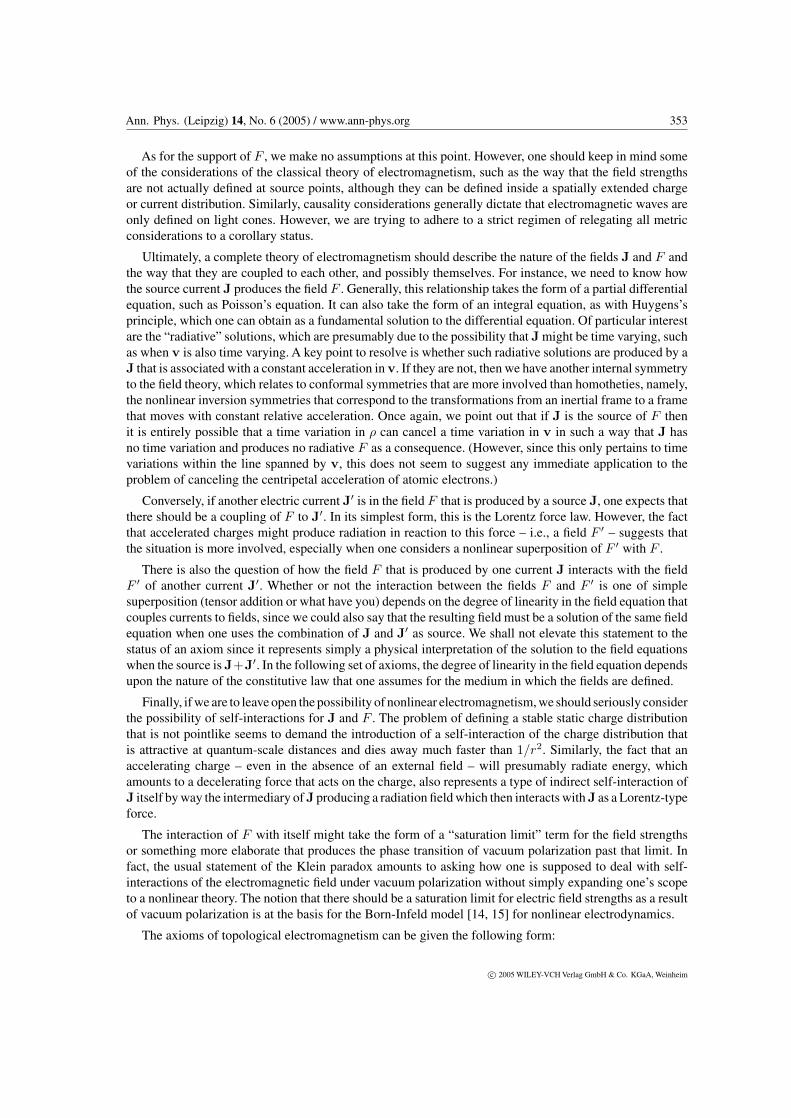
As for the support of F , we make no assumptions at this point. However, one should keep in mind someof the considerations of the classical theory of electromagnetism, such as the way that the field strengthsare not actually defined at source points, although they can be defined inside a spatially extended chargeor current distribution. Similarly, causality considerations generally dictate that electromagnetic waves areonly defined on light cones. However, we are trying to adhere to a strict regimen of relegating all metricconsiderations to a corollary status.

Ultimately, a complete theory of electromagnetism should describe the nature of the fields J and F andthe way that they are coupled to each other, and possibly themselves. For instance, we need to know howthe source current J produces the field F . Generally, this relationship takes the form of a partial differentialequation, such as Poisson’s equation. It can also take the form of an integral equation, as with Huygens’sprinciple, which one can obtain as a fundamental solution to the differential equation. Of particular interestare the “radiative” solutions, which are presumably due to the possibility that J might be time varying, suchas when v is also time varying. A key point to resolve is whether such radiative solutions are produced by aJ that is associated with a constant acceleration in v. If they are not, then we have another internal symmetryto the field theory, which relates to conformal symmetries that are more involved than homotheties, namely,the nonlinear inversion symmetries that correspond to the transformations from an inertial frame to a framethat moves with constant relative acceleration. Once again, we point out that if J is the source of F thenit is entirely possible that a time variation in ρ can cancel a time variation in v in such a way that J hasno time variation and produces no radiative F as a consequence. (However, since this only pertains to timevariations within the line spanned by v, this does not seem to suggest any immediate application to theproblem of canceling the centripetal acceleration of atomic electrons.)

Conversely, if another electric current J′ is in the field F that is produced by a source J, one expects thatthere should be a coupling of F to J′. In its simplest form, this is the Lorentz force law. However, the factthat accelerated charges might produce radiation in reaction to this force – i.e., a field F ′ – suggests thatthe situation is more involved, especially when one considers a nonlinear superposition of F ′ with F .

There is also the question of how the field F that is produced by one current J interacts with the fieldF ′ of another current J′. Whether or not the interaction between the fields F and F ′ is one of simplesuperposition (tensor addition or what have you) depends on the degree of linearity in the field equation thatcouples currents to fields, since we could also say that the resulting field must be a solution of the same fieldequation when one uses the combination of J and J′ as source. We shall not elevate this statement to thestatus of an axiom since it represents simply a physical interpretation of the solution to the field equationswhen the source is J+J′. In the following set of axioms, the degree of linearity in the field equation dependsupon the nature of the constitutive law that one assumes for the medium in which the fields are defined.

Finally, if we are to leave open the possibility of nonlinear electromagnetism, we should seriously considerthe possibility of self-interactions for J and F . The problem of defining a stable static charge distributionthat is not pointlike seems to demand the introduction of a self-interaction of the charge distribution thatis attractive at quantum-scale distances and dies away much faster than 1/r2. Similarly, the fact that anaccelerating charge – even in the absence of an external field – will presumably radiate energy, whichamounts to a decelerating force that acts on the charge, also represents a type of indirect self-interaction ofJ itself by way the intermediary of J producing a radiation field which then interacts with J as a Lorentz-typeforce.

The interaction of F with itself might take the form of a “saturation limit” term for the field strengthsor something more elaborate that produces the phase transition of vacuum polarization past that limit. Infact, the usual statement of the Klein paradox amounts to asking how one is supposed to deal with self-interactions of the electromagnetic field under vacuum polarization without simply expanding one’s scopeto a nonlinear theory. The notion that there should be a saturation limit for electric field strengths as a resultof vacuum polarization is at the basis for the Born-Infeld model [14, 15] for nonlinear electrodynamics.

The axioms of topological electromagnetism can be given the following form:



Axiom 1. Conservation of electric charge: J defines a homology class in H1(M ; R), i.e.:

δJ = 0. (3.2)

Axiom 2. Conservation of magnetic flux: F defines a cohomology class in H2(M ; R), i.e.:

dF = 0. (3.3)

Axiom 3. Constitutive law: There exists a smooth map that takes one of the following forms:

f : Λ2(M ; R) → Λ1(M ; R), F → J (3.4a)

f : Λ1(M ; R) × Λ2(M ; R) → C∞(M), f(F,J) = 0. (3.4b)

Furthermore, we make the following physical interpretations of certain geometric objects:

Physical interpretation 1. Lorentz force: The 1-form iJF represents the force that is exerted by the electro-magnetic field F on the current J. When J is the source of F this force is that of radiative reaction.

Physical interpretation 2. Superposition: When F is the field produced by a source J and F ′ is the fieldof a source J′ then the field that is produced by the source J + J′3 represents the (possibly nonlinear)superposition of the fields F and F ′.

Physical interpretation 3. Constitutive law. If the operator f = δ · χ for some diffeomorphism χ :Λ2(M ; R) → Λ2(M ; R) then the equations:

h = χ(F ) and δh = J (3.5)

complete the usual Maxwell equations, in which any nonlinearity would originate in the constitutive law χand reduces to linearity in the limiting case of weak field strengths.

In the paper of Hehl et al. [11], two other axioms were mentioned. In addition to the aforementionedthree axioms, it was suggested that one would need to postulate the existence of a proper time simultaneityfoliation [16] and raise the existence of a Lorentz force from the status of a physical interpretation to amathematical axiom. In the present formulation, the latter axiom is unnecessary because if J′ is anotherconserved current that is in the field F produced by the source current J then we can form the interiorproduct:

α = iJ′F (3.6)

with no further assumptions and interpret it as the force that F exerts on J′. Hence, we simply include theLorentz force as a physical interpretation, not an axiom.

As for the axiom concerning the existence of a proper time simultaneity foliation, which seems mostlydirected towards facilitating the definition of the electric and magnetic 1-forms that one obtains from Fwhen one chooses a rest frame, let us subdivide this issue into two sub-issues:

1. The existence of a Whitney sum decomposition of T (M) into L(M)⊕Σ(M), where L(M) is a (real)line bundle that represents a field of proper time directions and Σ(M) is a rank-three vector sub-bundle thatrepresents a distribution of spacelike tangent subspaces.

2. The integrability of the differential system on M that Σ(M) represents into a codimension foliationof M by proper time simultaneity submanifolds.

3 The sum in this expression refers to the addition of 1-chains. Of course, the carrier of the sum is the union of the carriers andthe coefficients at the points of their intersection is the vector sum, so this is still a vector addition, after all.



Although the subject at hand is discussed in more detail in [16], for now, we simply point out that such aWhitney sum decomposition is usually an artifact of defining a Lorentzian structure, by way of a choice of restframe. Since we are trying to exhibit the reduction from the SL(4) structure that facilitates electromagnetismto the bundle of oriented Lorentzian frames as a consequence of the axioms of electromagnetism, we shalltry to avoid introducing the axiom of such a decomposition from the outset.

However, we can say this much about Lorentzian structures and rest frames, a priori: All it takes todefine a Lorentzian structure, at least in the eyes of homotopy theory, is a line field, and one does have sucha Lorentzian structure on the set of points, NZ(J), at which J is non-zero; since this set is an open subsetof M , it is also a manifold. The line Lx(S) at every point x ∈ NZ(J) is then the one that is spanned by J atthat point. Furthermore, because the line field Lx(NZ(J)) was defined by a non-zero vector field to beginwith, it is an orientable line bundle. As for the matter of defining a Lorentzian pseudo-metric, it is importantto note that the homotopy equivalence of a global line field on M with a Lorentzian pseudo-metric g doesnot define a canonical association of one with the other. In effect, any 3-plane in each tangent space tox ∈ NZ(J) that does not contain the line Lx(NZ(J)) could serve as an orthogonal complement.

The line bundle L(NZ(J)) → NZ(J) also defines a rest frame for the motion of the charge distributionthat defines the current, namely the equivalence class of unit-volume linear frames at each point of NZ(J)that have one leg in Lx(NZ(J)). Since we have not specified which Lorentzian metric is associated withL(NZ(J)) we can only define a reduction of SL(M) to SL(3)(M) as a result of this. Similarly, without achoice of g we have no unique choice of complementary sub-bundle to L(NZ(J)) in T (NZ(J)). Hence, theintegrability of the 3+1 decomposition of T (NZ(J)) into a foliation of NZ(J) by proper time simultaneityleaves becomes moot.

Notice that when we state the integral forms of the first two axioms, namely:

J[V ] =∫

V

#J = 0 for any bounding three-dimensional region V (3.7a)

F [S] =∫

S

F = 0 for any bounding two-dimensional region S, (3.7b)

we cannot make the usual stipulations about whether these regions are spacelike, since we are trying torelegate such purely Lorentzian concerns to consequences of the electromagnetic structure.

If we look at the first axiom in differential form, we observe that when J = ρv it also takes the form ofa continuity equation:

0 = δJ = dρ(v) + ρδv (3.8)

or:

vρ = −ρδv, (3.9)

which can also take form:

δv = −v(ln ρ). (3.10)

This shows that v is incompressible iff ρ is constant along the flow of v. We shall return to the formalstructure of equation (3.10) in a different context.

The integral form of the first axiom then becomes:∫

N

v(ln ρ)V = −∫

N

d#v = −∫

V

#v. (3.11)

whenever V = ∂N .



If one interprets the functional F [S] as producing the total magnetic flux in an arbitrary compact orientable2-dimensional submanifold S then one sees that if S bounds, so S = ∂V , then this makes physicallyintuitive sense and implies that the total magnetic charge in V is 0. However, when S does not bound athree-dimensional region, although the total magnetic flux in S might well be non-zero, nevertheless, onecould not physically interpret the integral as the magnetic charge contained in a three-dimensional regionsince Gauss’s theorem would no longer apply.

Of course, since we are defining a source current as a one-dimensional homology class and an electro-magnetic field as a two-dimensional cohomology class one naturally must confront the question of whetherthere is only one such class or more than one, i.e., whether H1(M ; R) or H2(M ; R) vanishes. This naturallyleads into the subject of our next section.

Finally, one must point out that there is still something formally incomplete about our system of axiomsin that:

a) Ultimately it would be preferable to exhibit the fields F and J as having some intrinsic geometrical ortopological origin, instead of introducing them as essentially logical primitives.

b) The constitutive law also seems to lack an immediate relationship to either the geometry or topologyof the spacetime manifold.

Hence, the primary goals of refining the present axioms should probably be those of:

a) Exhibiting the spacetime metric and wave motion as special case corollaries to the constitutive laws.

b) Constructing the constitutive law from physical first principles and fundamental physical processes,as one might in the physics of condensed matter.

c) Illuminating a path into nonlinear electrodynamics that might define deeper foundations for quantumelectrodynamics.

d) Suggesting a promising Ansatz for exhibiting the fields F and J as being naturally associated withgeometrical or topological structures associated with the SL(4) reduction of the bundle of linear frameson spacetime that is necessary in order to facilitate Poincare duality.

4 Gauge symmetries and conservation laws

The reason for the use of the plural in the title of this section is that actually, we have two ways in whichambiguity can arise in the construction of our basic fields F and J. The first is the usual one that relates tothe possibility that the closed 2-form F is also exact; i.e., whether there exists a potential 1-form A suchthat:

F = dA. (4.1)

There are two comments that must be made about this: First: Whether or not such an A exists globallydepends upon the vanishing of H2(M ; R). If that module does not vanish then one can find only localpotential 1-forms. Second: If z is a closed 1-form then A + z is also a potential 1-form for F . This definesan equivalence class of 1-forms by the equivalence relation:

A ∼ A′ iff A − A′ ∈ Z1(M ; R). (4.2)

One refers to the equivalence relation as gauge equivalence and the transformation:

A → A + z (4.3)



as a gauge transformation of the second kind. In order to describe what the gauge transformations of thefirst kind were, we need to account for the appearance of the usual U(1) symmetry.

Customarily, one exhibits the closed form z as an exact form dλ, which means that zero-form λ representsa sort of infinitesimal generator for the gauge transformation. Naturally, the question of whether global zexist that are not exact depends upon the vanishing of H1(M ; R), which is essentially the question ofwhether M is simply connected. However, since the customary physical arguments are usually local inscope, the Poincare lemma allows us to find a suitable zero-form λ locally. This shows that the set ofinfinitesimal gauge transformations of the second kind can be effectively parameterized by the 0-forms.This means that we can regard the vector space of 0-forms as the (Abelian) Lie algebra of the group ofgauge transformations. Since the Lie algebra over R can define the infinitesimal transformations of eitherthe group (R+,×) or the circle group, which can also be considered as SO(2) or U(1), the group of gaugetransformations can be either the Lie group of positive smooth functions on M under multiplication, or theLie group of smooth functions from M into S1. Since the usual physical discussions of gauge field theoryare mostly concerned with infinitesimal transformations – those being the ones that define field variations– the choice of the Lie group (R+,×) or U(1) for finite transformations is one of physical intuition, andthis usually suggests that a gauge is like a phase; hence, the choice of U(1) is customary.

The traditional reasoning behind this is that quantum mechanics introduces a U(1) phase factor intothe description of any particle by wave functions, whether they are photons, whose position distributionsare obtained from complex wave functions, or electrons, whose position distributions are obtained fromspinor wave functions. However, just as introducing a metric into the theory of electromagnetism seemspremature when the metric should be a consequence of the propagation of electromagnetic waves, it alsoseems somewhat premature to introduce traditional quantum mechanical arguments into a theory that – onehopes – might shed new light on the deeper nature of quantum mechanics to begin with. Consequently, theauthor has been pursuing the possibility that the gauge structure for electromagnetism is not something oneintroduces axiomatically and independently from the geometry and topology of spacetime – as we alreadydid with the fields F and J themselves – but something that follows naturally from the demands of physicalinterpretation. In particular, obtaining the gauge structure as actually an SO(2)-reduction of the bundleof linear frames on M seems promising (see [17]). However, that discussion would take us far from theimmediate concerns, so we simply accept the traditional argument, for now, and proceed.

If we then give z the form (which is no loss of generality):

z = d(ln g) = g−1dg, (4.4)

where g: M → U(1), then, if we introduce a slight redundancy, the transformation (4.3) takes the form:

A → g−1Ag + g−1dg (4.5)

that one finds for the transformation of the local representative of a U(1) connection 1-form. One thenrefers to the group U(1) as a gauge group (of internal symmetries) for the field F and the choice of g(or z) as a choice of local U(1) gauge for F , since F is locally equivalent to the pair (A, z). This set ofassociations also carries with it the interpretation of F = dA as the curvature 2-form that is associated withthe connection 1-form A.

In order to complete this geometric picture, we need to account for the appearance of a U(1) principalbundle P → M on which the connection 1-form A would be defined; one generally refers to such a principalfibration as a gauge structure for the field theory. However, this gauge structure is usually constructedindependently of the bundle of linear frames on spacetime as an essentially auxiliary object.

If one forms the electromagnetic field Lagrangian:

L =12

dA(h) + A(J) (4.6)

one sees that as long as one assumes that the constitutive equation gives h as a function of F , and not A,then the kinetic energy term is gauge invariant. Under a gauge transformation, the interaction term A(J)



picks up a contribution of:

dλ(J) = Jλ. (4.7)

Since this does not always vanish, we see that the interaction term breaks the gauge invariance of L. ByNoether’s theorem, the U(1) internal symmetry of L is associated with a conserved current:

J =δLδA

, (4.8)

which means that the U(1) gauge symmetry is equivalent to charge conservation.A less-discussed form of gauge equivalence is the one that pertains to J when one addresses the question

of whether a super-potential h exists for J; i.e., an h ∈ H2(M ; R):

J = δh. (4.9)

By the homological Poincare lemma such an h always exists locally. Whether this is also possible globallyis a matter of whether H1(M ; R) vanishes.

By the Hurewicz isomorphism theorem, this comes down to whether M is simply connected or not. IfM is not simply connected, we could pass to the simply connected covering manifold M , where one wouldalways have the existence of a globally defined h. However, since a global section of the covering maps: M → M would have to represent a global orientation, when M is not orientable s will necessarily beundefined at some points of M . The same will then be true of the image of J in X(M), namely s∗J, as wellas the pull back of h to M by s, namely s∗h.

Once again, we see that h is not uniquely defined. Since δ2 = 0, if Z ∈ Z2(M ; R) is a co-closed 2-formthen the 2-form that one obtains by the transformation:

h → h + Z (4.10)

is also a superpotential for J. This defines a different sort of gauge equivalence for superpotentials:

h ∼ h′ iff h − h′ ∈ Z2(M ; R). (4.11)

Instead of looking for a 0-form to locally represent these transformations, we look for a 3-vector field Ksuch that Z = δK. By Poincare duality, K corresponds to a 1-form #K. Hence, the space of infinitesimalsuperpotential gauge transformations is parameterized by Λ1(M) this time. If we are only being local,we can exhibit these transformations by smooth functions from M to R

4. If we wish to regard this as theAbelian Lie algebra of some Lie group of functions from M to an Abelian Lie group G then one shouldobserve that R

4 can cover any of the Lie groups R4, S1 ×R

3, T 2 ×R2, T 3 ×R, T 4. This level of ambiguity

suggests that we are perhaps following the wrong ansatz. Furthermore, there is a fundamental differencebetween the ambiguity in h expressed by (4.11) and the gauge ambiguity in the potential 1-form for F : thecomponents of the electromagnetic induction bivector are physically measurable, but the introduction of apotential 1-form has a somewhat mathematically formal character.

Hence, rather than pursue the analogous reasoning that we followed for the aforementioned gaugetransformations, let us look at equation (3.10) again. This time, we shall put it into the form:

δv = −iv(ρ−1dρ). (4.12)

The 1-form ρ−1dρ takes the same form as the g−1dg term that appeared in the context of the gaugetransformations of A. We are then tempted to consider it to be a 1-form with values in the Lie algebra R.However, since we are dealing with vector fields with non-zero divergence, we suspect that this time R

is not the imaginary axis that generates the two-dimensional rotations, but the real axis that generates thedilatations, which is the multiplicative group R

+.



If we recall that ρ originated when we chose to decompose J, which is assumed to have zero divergence,into ρv then one could also say that, in effect, since this choice of decomposition for J depends upon thechoice of ρ, one must choose a dilatational gauge in order to define the vector field v. It is intriguing thatsuch a dilatational gauge is also associated with a choice of parameterization for an integral curve of v,which also relates to mass and kinetic energy. At the moment, though, our concern is how it relates to chargeconservation.

Now let us assume that ρ−1dρ is the 1-form that appears when one makes a change of local gauge on anR

+-principal bundle by way of ρ and transforms a local connection form σ from one gauge to the other:

ω → ρ−1σρ + ρ−1dρ. (4.13)

This time, we have no problem identifying the R+-principal bundle in question, since it is undoubtedly the

associated R+-principal bundle to L(NZ(J)), which consists of all positive scalar multiples of the vector

Jx at any point x ∈ M . We shall denote this R+-principal bundle by SL(NZ(J)). Ordinarily, a line field on

a manifold only defines an R∗(= R − 0)-principal bundle by way of the complement of its zero section.

In order to reduce this to an R+-principal bundle, we would need to first show that the line field is orientable

and then choose an orientation, which is simply a non-zero vector field on the support of the line field.However, this is also how we defined L(NZ(J)) in the first place, so the orientation is automatic. One mustnote that the bundle SL(NZ(J)) of unit volume 1-frames on NZ(J) is topologically uninteresting, sincethe existence of a global section (over NZ(J)) makes it trivial: SL(NZ(J)) = NZ(J) × R

+. Hence, anoriented one-frame on NZ(J) is equivalent to smooth function on NZ(J) with values in R

+. In particular,if v = λJ with λ > 0 then the function associated with the oriented 1-frame v is simply λ.

The question then becomes that of how we physically account for the appearance of a connection 1-formon SL(NZ(J)). To address this issue, we first consider the role that it plays. Since ρ seems to be relatedto the scaling of the vector field J within the oriented line field that it spans, the issue would seem to behow one compares the unit of (one-dimensional) “volume” in the fiber Lx(NZ(J)) at one point with theunit of volume at a neighboring point. (Of course, in dimension one a volume serves the same purpose asa norm or metric.) One must remember that in the absence of a metric there is nothing to distinguish any1-frame of L(NZ(J)) as having a “unit” volume, except when one makes such an association arbitrarily.Hence, if that choice is to be truly arbitrary then the scaling factor that takes any 1-frame to a rescaled onemust represent an internal symmetry of the field theory. However, one notes that in the conventional theoryof electromagnetism this homothety invariance is only true for the electromagnetic waves themselves andis broken by the introduction of a mass term.

The connection 1-form ω that we defined takes its values in R, which is the Lie algebra of (R+,×). Likethe electromagnetic potential 1-form, it too is an ordinary differential form. Consequently, we suspect thatthe only geometrical object that relates to it that also has an unambiguous physical meaning is its curvature,or field strength, 2-form:

Ω = dω. (4.14)

(The term ω ∧ ω vanishes because the Lie algebra of (R+,×) is Abelian.)Although it is tempting to speculate on whether Ω might relate, at least indirectly to the definition of

the 2-form F , keep in mind that Ω is defined only over NZ(J), whereas F is essentially defined on thecomplement of NZ(J). Hence, one would have to replace the definition of F with a further “topologicalconstitutive map”:

Λ2(NZ(J)) → Λ2(M − NZ(J)). (4.15)

In effect, this is what we usually get from solving the field equations: a map from the source to the field. Ofcourse, since we are defining Ω to be an exact form and F to be a closed form, if we pass to cohomologyand the induced map is linear it would only take [Ω] to 0, so unless [F ] = 0, as well – i.e., F = dA – weshould not expect this Ansatz to be productive in the context of topological electromagnetism unless thedefinition of Ω were weakened to something closed, but not exact.



5 The constitutive axiom

Naturally, the most open-ended axiom in the aforementioned set is the third one that concerns the existenceof an electromagnetic constitutive map. The problem is to leave open the possibility that the constitutive lawis nonlinear in such a way that it still relates to the geometrical or topological nature of the basic objects. Onemust unavoidably consider nonlinear theories of electromagnetism for both practical considerations, such asnonlinear optics, and more theoretical considerations, as when one is considering quantum electrodynamics.In either case, the domain of relevance tends to be the realm of large field strengths, such as the electric andmagnetic fields of high-energy laser beams, or the electric field of an electron or an atomic nucleus whenone is sufficiently close.

The existence of vacuum polarization in QED tends to suggest a nonlinear constitutive law for thespacetime vacuum itself. (For a lengthier discussion of such matters, see [18].) Since the constitutive lawsof macroscopic media are usually obtained by considering the macrostates (in the thermodynamic sense) thatfollow from the microstates of more fundamental processes, such as the formation of electric or magneticdipoles in charge distributions, this seems to be the most promising direction for trying to probe the natureof the constitutive law that governs the electromagnetic vacuum state.

In a topological theory of electromagnetism, one might also wish that the microstates in question containfundamental topological information. For instance, Misner and Wheeler [19] once attributed the appearanceof charge itself to the existence of the much-discussed “spacetime wormholes,” which amount to topologicalobjects that render H2(M ; R) non-trivial. An unacceptable aspect of the attachment of wormholes in theeyes of pre-metric electromagnetism is that they are three-dimensional objects that look like S1×S2 and areattached (by connected sum) to the three-dimensional spacelike leaves of a chosen proper time simultaneityfoliation. In fact, for the purposes of most spacetime models, if one regards spacetime as the Cauchydevelopment of an initial spatial manifold Σ then the foliation is the “cylindrical” foliation M = R × Σ.In the absence of such a foliation, one can only attach four-dimensional objects to a four-dimensionalmanifold by connected sum and still produce a manifold. If one attaches, say, a point or a curve segmentand wishes to still produce a four-dimensional manifold, one must make some further identifications andpass to a quotient, such as attaching the point at infinity to a plane by stereographic projection. Later, weshall discuss topological matters in the context of constitutive laws.

As we have defined the term, a constitutive law will generally be a differential equation in the two fieldsJ and F . However, as pointed out above, this equation may factor through an essentially algebraic map h:Λ2(M) → Λ2(M) and the codifferential δ – i.e., δh = J – which is the traditional form.

One can appeal to the theory of gravitation for an analogy. The spirit of Sakharov’s notion of gravitationas “metrical elasticity” is that if spacetime curvature is essentially related to the second covariant derivativeof the strain that is associated with deforming the Minkowski metric ηµν into the Lorentzian metric gµν

– a la the Cauchy-Green conception of the strain tensor, which would amount to gµν − ηµν – and this iscoupled to stress-energy-momentum tensor then the Einstein field equations take the form of a constitutiveequation in differential form.

One can give the electromagnetic constitutive axiom different forms, depending upon whether oneassumes that F = dA for some A ∈ Λ1(M ; R) or J = δh for some h ∈ Λ2(M ; R). For instance, in theformer case, one might consider laws of the form:

A = A(J), J = J(A), f(A,J) = const. (5.1)

In the latter case, one might consider laws of the form:

F = F (h), h = h(F ), f(F, h) = const. (5.2)

In (5.1), the last expression represents a common form for the interaction term A∧#J = (AµJµ)V in theelectromagnetic Lagrangian that expresses how the source current gets coupled to the electromagnetic field.Similarly, the last expression of (5.2) is of the form of the field kinetic energy term 1

2 F ∧#h = ( 14 Fµνhµν)V

in such a Lagrangian.



Hence, we form the expressions:

12

F∧#h =12

F (h)V, A∧#J = A(J)V, (5.3)

which are actually equivalent to forming:

12

F∧H, A∧∗J, (5.4)

when one deals with H as a 2-form and J as a 3-form. However, the latter form requires the introduction ofa metric in order to associate the vector field J with the 1-form J and the bivector field h with the 2-formH . Later, we shall examine the expression F∧H in the context of the intersection form of the spacetimemanifold.

In local components, and neglecting the factor of V , (5.3) gives the usual expressions:

Lkin =14

Fµνhµν , Lint = AµJµ. (5.5)

The 2-vector field h of electromagnetic induction is the one that appears in the Maxwell equations, whenwe give them the form:

dF = 0, δh = J, h = h(F ), (5.6)

The homological Poincare lemma says that one can, at least locally, find a 2-vector field h such that:

J = δh. (5.7)

Of course, in the present case, as opposed to the usual machinery of Maxwell’s equations in terms ofdifferential forms, h is a 2-vector field, instead of a 2-form. However, this was always implicit when onewrote the Maxwell equations in the older local – but still metric-free – form:

∂µFνλ + ∂νFλµ + ∂λFµν = 0, ∂µhµν = Jν , hµν = hµν(Fµν). (5.8)

The situation that is associated with the existence of a global h on a manifold is simpler than the situationthat relates to the existence of a global potential 1-form A such that F = dA. In the former case, wherethe issue is the vanishing of H1(M ; R), one can define one’s fundamental fields F , J, h on the simplyconnected covering manifold of M and pull them down to subsets of M by way of local orientations. Inthe latter scenario, the issue is the vanishing of H2(M ; R), which cannot be sidestepped by passing to acovering manifold, and leads to the possible existence of magnetic monopoles and spacetime wormholes.

If one is given the Lagrangian L = L(F,J) a priori then one can retrieve the constitutive law from:

h =∂L∂F

. (5.9)

If we sense that we are close to dealing with a spacetime metric then that is due to the fact that we areconcerned with a kinetic energy, and, as one knows from relativistic point mechanics, kinetic energy is, inits simplest form, conformally related to the spacetime metric. Furthermore, the conformal factor is simplythe rest mass of the point particle; of course, in the case of electromagnetic waves this conformal factorwould be zero.

Another piece of the geometric puzzle that is associated with constitutive laws comes from the fact thatthe speed of propagation of electromagnetic waves in vacuo – i.e., c0 – is actually a derived quantity thatfollows from the assumed form of the constitutive law for the classical electromagnetic vacuum. That law



amounts to the assumption that the electric and magnetic polarizability of that state is expressed by twoconstants, ε0 and µ0, which give:4

c20 =

1ε0µ0

. (5.10)

As is well known, one of the most far-reaching consequences of quantum electrodynamics is the suggestionthat this aforementioned assumption is an oversimplification of the nature of the electromagnetic vacuumstate. In particular, vacuum polarization seems to contribute at every turn to the nature of elementaryelectromagnetic processes at the quantum level. Consequently, one expects that if classical electromagnetismleads to gravitation somehow then quantum electrodynamics might lead to quantum gravity (or at least anunambiguous definition of the concept). Alternatively, if that is not the case then perhaps it is only quantumelectrodynamics that leads to gravitation in the first place; indeed, this is probably more likely.

An intriguing hint of how this might come to pass is given by the fact that (5.10) also suggests that onecan rewrite the simplest spacetime metric – i.e., the Minkowski space metric – in the form:

ηµν = diag(

1ε0µ0

,−1,−1,−1)

=1ε0

diag(

1µ0

,−ε0,−ε0,−ε0

). (5.11)

In this one elementary geometrical object, we can see Ansatze that might lead to the unification ofgravitation, electromagnetism, vacuum polarization, and wave mechanics.

In order to gain more intuition about the nature of the problem of how the electromagnetic constitutivemodel leads to the spacetime metric as a consequence, we examine two special cases of an electromagneticconstitutive model: the linear case and the nonlinear case as it relates to nonlinear optics and the Born-Infeldmodel, which they constructed in order to account for vacuum polarization effects to some degree. We thenmake some observations and speculations on the problem of resolving the constitutive laws into geometricaland topological aspects of more fundamental processes.

5.1 Linear case

In conventional linear electrodynamics one ordinarily assumes the a priori existence of a Lorentzian metricg, so the constitutive relation takes the 2-form F to the 2-form H by way of:

H(F ) = (ιg × ιg) · χ(F ), (5.12)

where:

ιg : T (M) → T ∗(M), v → ivg (5.13)

is the linear isomorphism that takes each tangent vector to its metric-dual covector and:

χ : Λ2(M) → Λ2(M), F → h = χ(F ) (5.14)

is a linear isomorphism of 2-forms with 2-vector fields. In this form, we see that in an unpolarized mediumthe correspondence (5.12) is simply the identity map and one should have simply:

χ = (ιg × ιg)−1. (5.15)

We then see that the effect of polarization is to deform the isomorphism of Λ2(M) with Λ2(M) that isdefined when one has a Lorentzian metric g. One might even consider the possibility that this deformationoriginates in a deformation of the metric itself, g → g′ = g + δg, which should make:

ιg′ × ιg′ = ιg × ιg + ιδg × ιg + ιg × ιδg + ιδg × ιδg. (5.16)

4 Although the units in which c0 = 1 are sometimes called “God’s units,” the fact that they tend to obscure the deeper truth ofthis physical subtlety suggests that they are probably “Satan’s units,” since God does not play games with truth.



We could then define the polarization tensor field p to be the difference between the deformed andundeformed states:

p = (ιg′ × ιg′)−1 − (ιg × ιg)−1. (5.17)

To relate this to the usual definition of the polarization tensor field we define:

P = (ιg × ιg)p = (ιg × ιg)(ιg′ × ιg′)−1 − I, (5.18)

which agrees with the usual conception of the polarization tensor field as H − I if we set:5

H = (ιg × ιg)(ιg′ × ιg′)−1 = (ιg × ιg)χ. (5.19)

Relative to a natural frame field, (5.12) takes the component form:

Hµν = gµρgνσhρσ = gµρgνσχρστυFτυ. (5.20)

We can then represent the matrix of the map g∧g = (ιg × ιg) by way of:

(g∧g)µρνσ =12

(gµρgνσ − gνρgµσ). (5.21)

When we are dealing with an oriented Lorentzian manifold, in addition to the isomorphism of Λ2(M) withitself that is defined by (ιg × ιg) ·χ, we also get another isomorphism from (the inverse of) Poincare duality.If we compose the maps χ and # then we get the isomorphism:

∗χ : Λ2(M) → Λ2(M), F → #χ(F ). (5.22)

We must be careful to distinguish the effect of this map from the previous one defined by (ιg × ιg) · χ. Inthe limit of an unpolarized medium χ goes to (ιg × ιg)−1 so the map (ιg × ιg) · χ goes to I , but the map ∗

χ

goes to the conventional form of the Hodge star isomorphism on a pseudo-Riemannian manifold. Hence,∗χ is a deformation of the Hodge star isomorphism due to polarization.

We now wish to eliminate the explicit reference to the metric in the aforementioned constructions. Wefirst represent the electromagnetic induction by the 2-vector field h = χ(F ), instead of the 2-form H .Furthermore, we can alternatively represent the tensor field χ by the fully contravariant fourth rank tensorfield of the form χ ∈ Λ2(M) ⊗ Λ2(M) that corresponds to the linear isomorphism (5.14).

The components of a tensor field of the form χ ∈ Λ2(M)⊗Λ2(M) come with two symmetries already:First, there is antisymmetry in the first and last pair due to the fact that they pertain to 2-forms. Second,from Lagrangian considerations, one often assumes that there is also a transposition symmetry of the form:

χ(α, •) = χ(•, α), α ∈ Λ2(M). (5.23)

This corresponds to a symmetry in the components of χ:

χµντυ = χτυµν . (5.24)

This latter symmetry, combined with the fact that χ is a bilinear and non-degenerate functional on the vectorbundle Λ2(M), implies that we can also regard χ as a fiber metric on the vector bundle Λ2(M). The questionthen arises: under what circumstances can we resolve the fiber metric χ on Λ2(M) to a Lorentzian one, g,on Λ1(M) = T (M)? From (5.21), which we rewrite as χ = g∧g, we see that we are essentially lookingfor the “exterior square root” of χ.

5 In this expression, we intend that H be considered as an operator.



From the orientability of M , if we choose a unit-volume element V = 14! ε

µνρσ∂∧µ ∂∧

ν ∂∧ρ ∂σ in T ∗(M),

i.e., a globally non-zero 4-vector field V on M , then one already has another scalar product defined for2-forms on an orientable M :

〈F, G〉 = V(F∧G) =12

εµνρσFµνGρσ. (5.25)

However, a simple comparison of symmetries shows that V cannot be represented by an exterior product ofsymmetric tensor fields, such as g∧g. Hence, if we wish to take the exterior square root of χ then we mustsubtract off the contribution proportional to V:

χ0 = χ − αV, (5.26)

for some appropriate scalar α.In order to find an exterior square root of χ0, we follow Hehl, et al. [11, 12] and define:6

∗ = #χ0 = #χ + αI, (5.27)

which is a linear isomorphism of Λ2(M) with itself.The square of # is:

∗2 = #χ0#χ0. (5.28)

If we can find a form for χ0 that satisfies the constraint:

∗2 = −1 (5.29)

then we expect that we have reproduced the Hodge isomorphism, at least for 2-forms.In order to solve (5.28) for χ0, at least locally, we choose a local frame field eµ whose domain is an open

subset U ⊂ M and whose reciprocal coframe field is θµ. We enumerate the basis for Λ2(U) defined by allθµ ∧ θν with µ < ν by EI , I = 1, 2, . . ., 6. We can express the matrices of # and χ0 as block matrices:

[#]IJ =

0 I

I 0

, [χ0]IJ =

A C

CT B

, (5.30)

in which A and B are symmetric 3 × 3 real matrices. For the general solution of (5.28), A and C must takethe form:

A = pB−1 − 1det B

N, C = B−1K (5.31)

in which K is an arbitrary antisymmetric 3×3 real matrix, which we express as ad(k) for a k ∈ R3, where

ad refers to the Lie algebra on R3 that is defined by cross product, and:

N = k ⊗ k, p =tr(NB)det B

− 1. (5.32)

If one has a tensor field χ0 that satisfies (5.28) then one can then decompose Λ2(M) into a direct sumΛ+2(M) ⊕ Λ−2(M) of rank-three sub-bundles by polarization:7

F = F+ + F− =12

(F −∗F ) +12

(F +∗F ). (5.33)

6 In order to stay consistent with our notation, which is based in a common notation for Poincare duality, we shall invert theiruse of # and ∗, though.

7 Note the non-intuitive sign convention.



One refers to the sub-bundles Λ+2(M) and Λ−2(M) as consisting of self-dual and anti-self-dual 2-forms,respectively, even though the eigenvalues are imaginary, not real, as in the Riemannian case.

Now, one can associate a conformal class of Riemannian metrics with every splitting of Λ2(M) into adirect sum Λ+(M) ⊕ Λ−(M) whose constituent sub-bundles have the same rank – viz., three. In fact, thiscorresponds to the splitting of Spin(4) into SU(2)×SU(2). It also relates to the fact the Hodge isomorphismis the same for all metrics in a conformal class.

Of course, the issue at hand is not to find a conformal class of Riemannian metrics, but a conformal classof Lorentzian metrics. As we have pointed out above, the existence of the former does not have to implythe existence of the latter. Similarly, the uniqueness of Riemannian metrics up to homotopy – they are allobtained by deformation retractions of the bundle of linear frames – does not imply the uniqueness of thehomotopy class of Lorentzian metrics, which depends upon the vanishing of H3(M ; Z2). Furthermore, thespin group that is associated with SO(3, 1), namely, SL(2; C), does not split the same way as Spin(4).However, if one regards a Lorentz boost Bas a “Wick-rotated” Euclidian rotation R:

B = w−1Rw, w = diag(1, i, i, i) (5.34)

then, at the infinitesimal level, the decomposition of the Lie algebra so(4) = so(3) ⊕ so(3) becomes thevector space decomposition of the Lie algebra so(3, 1) = so(3) ⊕ b(3), where the vector subspace:

b(3) = w−1so(3)w (5.35)

of infinitesimal boosts is not actually a Lie subalgebra of so(3, 1). The next question is whether we alsohave:

sl(2; C) ∼= su(2) ⊕ b′(2), (5.36)

where b′(2) is a three-dimensional subspace of infinitesimal boosts that one can obtain from su(2) bya linear isomorphism. The answer is straightforward: By Hermitian polarization, we can decompose anya ∈ sl(2; C) into a sum of a traceless Hermitian matrix and a traceless skew-Hermitian matrix:

a = h+ + h− =12

(h + h†) +12

(h − h†). (5.37)

Since the traceless skew-Hermitian part is an element of the Lie algebra su(2), we need only verifythat the traceless Hermitian part represents an infinitesimal boost and can be obtained from a tracelessskew-Hermitian matrix by a linear isomorphism. The first part follows from the isomorphism of sl(2; C)with so(3, 1) = so(3) ⊕ b(3). As for the second part, the usual way to associate a Hermitian matrix witha skew-Hermitian one is to take h− to −ih−. We cannot actually represent this by a conjugation, so wesimply regard the transformation defined by multiplying Hermitian matrices by i as the sl(2; C) equivalentof the Wick rotation. We represent this situation by the commutative diagram:

so(3)⊕so(3) so(3)⊕b(3)

su(2)⊕su(2) su(2)⊕b(2)

I⊕Ad(w )

Ι⊕−iFig. 1 Real and complex forms of the infinitesimal Wick rota-tion.

in which the vertical arrows are the complexifications.



Hence, we conclude that a splitting Λ2(M) = Λ2+(M) ⊕ Λ2−(M) is associated with a conformalclass [g] of Lorentzian pseudo-metrics, up to topological obstructions. (For the actual construction of arepresentative g from B, N, K, see Hehl, et al. [11].) This is equivalent to a global field of light cones onM .

In summation, we see that in the case of linear constitutive laws the assumption of symmetry in the tensorχ, when regarded as a non-degenerate bilinear form on Λ2(M), defines χ as a fiber metric on that vectorbundle. This, in turn, gives a splitting Λ2(M) = Λ2+(M) ⊕ Λ2−(M) defined by the polarization of any2-form by ∗ = #χ0, and if the existence of a global Lorentzian metric on M is topologically unobstructedthen this leads to a conformal class [g] of Lorentzian pseudo-metrics. Otherwise, when M is compact onewill have to restrict one’s consideration to an open submanifold of M that represents the complement of afinite set of points at which [g] is undefined. (If M is not compact then there is no topological obstructionto a global Lorentzian metric.)

Before we leave the realm of linear constitutive laws, we pause to point out another mathematicallyintriguing aspect of constitutive laws as scalar products on Λ2(M): Because the linear automorphism onΛ2(M) that is defined by ∗ = #χ0 has the property that ∗2 = −1, it defines an almost-complex structureon Λ2(M). In effect, the splitting Λ2(M) = Λ2+(M) ⊕ Λ2−(M) into self-dual and anti-self-dual 2-formsis analogous to their splitting into real and imaginary parts. Since the vector bundle Λ2(M) is of rank six asa real vector bundle, it will be of rank three as a complex vector bundle. This implies that its structure groupis GL(3; C). If one introduces an orientation and a Hermitian structure on Λ2(M) then one can reduceits structure group to SU(3). In fact, the orientation on T (M) implies an orientation on Λ2(M), and thescalar product χ defines a Hermitian structure by way of χ(α, β†) where β† = Re (β) − Im (β), in whichβ = Re (β) + Im (β) is the decomposition of β into self-dual and anti-self-dual parts. All of this mightsuggest a possible geometrical representation for the color SU(3) gauge structure of the strong interactionwithout the necessity of representing M as a complex three-manifold. However, our immediate concern iselectromagnetism, so we let that pass.

5.2 Nonlinear constitutive laws

We might extend our constitutive law from a linear one to something that is homotopic to linear; i.e.,something of the form:

χ(F ) = χ(1)(F ) + Ns(F ) (5.38)

in which χ(1) : Λ2(M) → Λ2(M) is linear, Ns : Λ2(M) → Λ2(M) is nonlinear with s ∈ [0, 1], and:

lims→0

Ns = 0. (5.39)

In such a case, we are dealing with a constitutive law of the “generalized Taylor series” form: linearmap + (nonlinear map that vanishes in the weak field limit). In nonlinear optics [20, 21], this level ofapproximation is referred to as “weak nonlinearity.” The next levels of approximation are the quadratic andcubic ones:8

χ(F ) = χ(0) + χ(1)(F ) + χ(2)s (F F ) (5.40a)

χ(F ) = χ(0) + χ(1)(F ) + χ(2)s (F · F ) + χ(3)

s (F F F ). (5.40b)

The leading constant term χ(0) subsumes any residual polarization of the medium that remains whenthere is no applied electromagnetic field. Although that sounds physically uninteresting in the case of theclassical spacetime electromagnetic vacuum, one should keep in mind that the Casimir effect is indicativeof the reality of the zero-point field that one expects from quantum electrodynamic considerations. If one

8 The notation refers to the symmetrized tensor product.



takes the position that quantum electrodynamics is really a phenomenological process for constructing theextension of linear electrodynamics into nonlinear electrodynamics in the realm of strong field strengths(see the “neoclassical” discussion in [18] or the quantum discussion in [22]) then one might still give thisterm serious consideration even for the electromagnetic vacuum.

The terms χ(2)s and χ

(3)s are linear maps from the respective symmetrized tensor products of Λ2(M)

with itself to Λ2(M). Hence, they can be represented in either form:

χ(2)s : Λ2(M) Λ2(M) → Λ2(M), (5.41a)

or:

χ(2)s ∈ Λ2(M) Λ2(M) ⊗ Λ2(M), (5.41b)

and:

χ(3)s : Λ2(M) Λ2(M) Λ2(M) → Λ2(M), (5.42a)

or:

χ(3)s ∈ Λ2(M) Λ2(M) Λ2(M) ⊗ Λ2(M). (5.42b)

Furthermore, χ(2)s and χ

(3)s are expected to vanish in the limit s → 0, which one intends to be the limit of

weak field strength. Hence, s represents a sort of coupling constant for the nonlinear terms.Although it would be mathematically natural to generalize all of this to the methodology of jet bundles

or covariant derivatives in order to account for the successive terms as true higher-order derivatives of hwith respect to F , we shall take a more nonlinear optical route and treat the successive terms as simplyphenomenologically defined tensor fields. Of course, the ultimate challenge to theoretical physics is toaccount for these tensor fields in terms of geometrically or topologically defined tensor fields; i.e., in termsof spacetime structure. Consequently, one should not keep the aforementioned generalities out of one’sconsideration completely.

In nonlinear optics, since:9

H(F ) = F + P (F ) = (I + P )(F ), (5.43)

one correspondingly regards the polarization 2-form P (F ) as the essential part in the eyes of nonlinearanalysis and then decomposes the nonlinear operator P into linear, quadratic, etc., parts:

P (F ) = P (0) + χ(1)(F ) + χ2(F F ) (5.44a)

P (F ) = P (0) + χ(1)(F ) + χ2(F F ) + χ3(F F F ). (5.44b)

However, since we are trying to avoid using the spacetime metric in the fundamental statements aboutelectromagnetism, and P seems to relate mostly to deformations of the metric, we shall simply regard(5.41a,b) as the approach we shall take to weak nonlinearity.

Of all of the effective theories of nonlinear electrodynamics that are based in quantum electrodynamicalconsiderations the one that seems to get the most attention is the Born-Infeld theory [14, 15]. It is based inthe imposition of a maximal field strength that would precede the onset of vacuum polarization, as in QED.

9 To be truly faithful to nonlinear optics, we should be talking about the electric field by itself, not the Minkowski 2-form, sincethe effects of large magnetic field strengths are usually treated as a separate class of phenomena. However, since our opticalmedium is the spacetime vacuum, and the E −B decomposition follows from the imposition of a metric and a time orientation,we shall be more cautious from the outset.



The Born-Infeld Lagrangian for the electromagnetic field F takes the form:

L = (√

E2c + F − G − Ec)V, (5.45)

in which Ec represents a critical electric field strength.In order to define the Born-Infeld Lagrangian, one must first introduce the field invariants:

I1 = F∧∗F = FV, I2 = F∧F = V(F, F )V = GV. (5.46)

These correspond to the local expressions:

F =12

gµνgρσFµνFρσ, G = εµνρσFµνFρσ. (5.47)

Ordinarily, one intends that the ∗ isomorphism is due to Hodge duality, which, in turn, comes fromthe imposition of a Lorentzian structure on spacetime, which is why one usually constructs one’s fieldLagrangian from Lorentz invariant expressions in F – a la Mie [26]. In the pre-metric case, one must lookfor SL(4)-invariant expressions. Of the latter two expressions, only I2 can be formed without introducinga metric, at least as stated. Indeed, it can be defined (as a 4-form) without recourse to V , so it is actuallyGL(4)-invariant. The expression F takes the form of ||F ||2 when one gives Λ2(M) the norm that comesfrom the scalar product g∧g.

However, recall that if we are considering a χ such that ∗2 = −1, where ∗ = #χ then, in effect, we havereconstructed the Hodge star, which is equivalent to a conformal class of metrics. Consequently, given sucha χ we can still use the ∗ isomorphism it defines in place of the Hodge star, and define a generalization ofI1 by:

I1 = F∧∗F = χ(F, F )V. (5.48)

However, since we have defined our replacement for the Hodge star only on 2-forms, none of theremaining three Lorentz invariants that Mie (with a correction from Weyl and Born) obtained, namely:

I3 = A∧∗A (5.49a)

I4 = iAF∧∗(iAF ) (5.49b)

I5 = iA∗F∧ ∗(iA ∗F ) (5.49c)

can be defined without using a metric, since they all take the form of norm-squares of 1-forms.The Lagrangians that involve norm-squares using the spacetime metric usually represent kinetic energy

terms for the field, just as the elementary expression for the non-relativistic kinetic energy of a pointmass involves using a conformal transform of the spatial metric tensor, whose conformal factor is 1/2m.Similarly, the potential energy in a one-dimensional (or isotropic three-dimensional) Hookean material thathas been displaced ∆x from its equilibrium state involves a conformal transform of the spatial metric whoseconformal factor is 1/2k.

However, when one goes from point matter to extended matter, or isotropic to anisotropic media, or linearto nonlinear media, all of the aforementioned simplifications break down and the conformal transformationof the metric must be – in the linear case – replaced with a product of a conformal transformation and avolume-preserving shear, and with more elaborate expressions when one goes to the nonlinear realm.

In any event, the generalizations all amount to constitutive laws in one form or another. A metric tensorthen emerges as essentially a special case of a process by which one associates tensor fields with their dualtensor fields. As we have seen, in the case of 2-forms on a four-manifold, a volume element gives another.



6 Topological constitutive laws

In order to make electromagnetism a completely topological phenomenon, in addition to giving a topologicalinterpretation to the fundamental fields, we also need to find some topological origin for the constitutiveproperties of the medium in question. This is especially perplexing in the case of the spacetime vacuumitself, since, classically, the spacetime vacuum was assumed to have an electromagnetic structure that wasexpressed only by the constants ε0 and µ0. However, as pointed out above, quantum electrodynamicssuggests that this picture of the spacetime vacuum is an oversimplification.

6.1 The intersection form

Since we are replacing our electromagnetic field strength 2-form F with its de Rham cohomology class[F ], we might also consider a constitutive axiom in the form of a bilinear functional on the second de Rhamcohomology space itself, instead of Λ2(M):

H2(M ; R) × H2(M ; R) → R. (6.1)

Note that this time we are defining our bilinear functional on a vector space, not a C∞(M)-module, as wedid for linear constitutive laws.

Now, any closed oriented orientable 4-manifold M already has one such functional defined by Poincareduality:

Q([α], [β]) =∫

M

α∧β = Q([β], [α]). (6.2)

Inside the integral, α and β are any closed 2-forms that define each chosen de Rham class in dimensiontwo. When M has no boundary, the integral will be independent of this choice of representative. If M has aboundary then, by Stokes’s theorem, replacing α by α + dλ and β by β + dµ will produce a boundary termof α∧µ−λ∧β+dλ∧µ, which does not have to vanish, except for a restricted class of gauge transformations,such as λ, µ that vanish on ∂M .

What is not entirely obvious in (6.2) is how Poincare duality and the choice of V affects the definitionof Q. Hence, we rewrite it as:

Q([α], [β]) =∫

M

α(∗β)V, (6.3)

in which the role of our choice of V and its associated Poincare duality isomorphism ∗ becomes clear.Q is not only non-degenerate, but unimodular, as well, so its symmetry and bilinearity imply that Q

defines a scalar product on the vector space H2(M ; R). The bilinear functional Q is called the intersectionform for a closed orientable M [10, 26–28]. As we shall see shortly, it plays a fundamental role in thetopology of four-dimensional differentiable manifolds.

The relevance of the intersection form to electromagnetism should be unavoidable in our present formu-lation, since we are defining electromagnetic fields to be two-dimensional de Rham cohomology classesto begin with. Of course, the only way that Q is non-trivial is if we assume that the topology of M has anon-vanishing H2(M ; R), i.e., that some F ’s do not admit global potential 1-forms, which gets one backinto the realm of magnetic monopoles, wormholes, and other spacetime pathologies. Hence, we brieflysummarize some of the fundamental features of the role that the intersection form plays in the topology offour-manifolds.

6.2 The topology of four-manifolds [26–28]

Algebraically, a scalar product can be classified by two integers: its rank, which equals the second Bettinumber for M in the present case:

b2 = dim(H2(M ; R)), (6.4)



and its signature:

τ = b+ − b−. (6.5)

where b+ is the maximal dimension of the subspaces of H2(M ; R) on which Q is positive definite and b−

is the maximum dimension of the subspaces on which it is negative definite.When one restricts the form Q to the free part of the integer cohomology, i.e., the free part of H2(M ; Z),

which defines an integer lattice of the form Zb2 , one can also define the type of Q according to whether it

takes it values in the even integers or not. In the affirmative case one calls Q even, and in the contrary caseone calls Q odd (although that does not have to imply that all of its values are odd integers).

For indefinite forms, the Hasse-Minkowski classification says:

Q =

Il ⊕ (−Im) when Q is odd

l

0 1

1 0

⊕ mE8 when Q is even.

(6.6)

In this classification, the matrix E8 is the Cartan matrix of the exceptional simple Lie algebra E8.For definite forms, the classification is not as straightforward. However, as we shall discuss later, Don-

aldson’s theorem narrows down the field of definite forms that describe the intersection forms of simplyconnected closed four-manifolds considerably.

For simply connected four-dimensional manifolds, the intersection form is fundamental to the othercharacteristic classes, since they can all be derived from the information that is contained in Q:

Second Stiefel-Whitney: Q(w2[M ], α) = Q(α, α)(mod 2) for all α ∈ H2(M ; Z2)First Pontrjagin:10 p1[M ] = 3τ [V] = 3(b+ − b−)[V]Euler: e[M ] = (b+b−)[V].

(In these expressions, V is a choice of unit volume element.) The first and third Stiefel-Whitney classesvanish by simple connectedness and Poincare duality; indeed this is actually true of w3 for any compactorientable 4-manifold. The fourth Stiefel-Whitney class is the Z2 reduction of e[M ].

The second Stiefel-Whitney class plays an important role in the context of Spin(4) structures on M ,namely it must vanish in order for an SO(4)-reduction of GL(M) to admit a two-to-one covering by aSpin(4)-principal bundle. Moreover, the homotopy classes of such bundles are indexed by H1(M ; Z2). Inparticular, if a simply connected four-manifold admits a spin structure then it must be unique. Moreover, asimply connected four-manifold admits a spin structure iff its intersection form, when restricted to integercohomology classes, takes on only even values.

The mathematician’s understanding of how the intersection form Q relates to the topology of simplyconnected four-manifolds is growing quite extensive by now. In 1949, Whitehead showed that if two closedsimply connected four-manifolds have isomorphic intersection forms then they are homotopy equivalent.In fact, every unimodular symmetric bilinear form is the intersection form of some simply connectedtopological four-manifold. However, not all of them will be smoothable, or even piecewise-linear.

For the case of indefinite intersection forms, one has mostly examples to deal with. For instance, onecan construct a compact orientable four-manifold with an intersection form diag(1, . . ., 1,−1, . . .,−1) =l(1)⊕m(−1) by taking the connected sum of l copies of CP2 (regarded as a real four-dimensional manifoldinstead of a complex two-dimensional one) with one orientation with m copies of CP2, which is CP2 withthe opposite orientation. This is because H2(CP2; Z) = Z, reversing the orientation inverts the sign of the

10 This result follows from either the Hirzebruch signature theorem [10, 29], or, more generally, the Atiyah-singer index theorem[29, 30].



intersection form, and the connected sum operation produces a direct sum in the cohomology. We point outthat the standard generator for H2(CP2; Z) is essentially CP1, which is diffeomorphic to a 2-sphere.

For the case of definite intersection forms, one has Donaldson’s celebrated theorem that the only positivedefinite intersection form on a smooth closed simply connected four-manifold is the standard one.

Now that we have discussed the notion of the intersection form of an orientable manifold, we can examineone possibility for rendering H2(M ; R) non-trivial in a manner that seems closely related to the physicalprocess of vacuum polarization in the presence of strong electric field strengths.

6.3 A possible topological mechanism for vacuum polarization

As a first attempt at giving a deeper physical basis for a topological constitutive axiom let us take the processof vacuum polarization literally and see what sort of expressions we can derive from it.

The basic process in vacuum polarization is that of the conversion of a photon into a virtual elec-tron/positron pair when the field strengths of the photon exceed some threshold value. We first assume thatthe reason for using the word “virtual” is simply the fact that these processes and their inverses may behappening over such a short time interval that the measurement process cannot resolve them in experimen-tal practice, even though their collective effect as a macroscopic ensemble is measurable; for instance, theLamb shift. Hence, a virtual process might represent a real, but unobservable, process.

We assume that any sufficiently small region of the spacetime electromagnetic vacuum can exist in oneof three phases:

a) Unpolarized; this is the weak field case.

b) Polarized by a bound electron/positron pair; this is the critical field case.

c) Stably charged, when the binding energy has been exceeded and the charges form stable disjointdistributions; we shall call this the super-critical field case.

Our main concern in this study is the transition between the first two phases, although we shall treat bothphase transitions as if they were associated with the spontaneous breaking of the vacuum symmetry and theappearance of topological defects.

We next observe that when a photon resolves to a bound electron/positron pair, as long as the two chargesare assumed to be separated by an actual displacement vector d there is also an electric dipole 2ed that isassociated with the pair. The vector d brings about a reduction in the symmetry of the vacuum state fromthe SO(2) gauge symmetry of the electromagnetic Lagrangian that represents charge conservation to thee symmetry of the vacuum state that a choice of non-zero vector brings about. The homogeneous spacethat is defined by this reduction is also SO(2) – or S1, if you prefer – whose first non-trivial homotopygroup is π1(S1) = Z. Hence, one should expect the topological obstruction to making such a reduction tobe an element of H2(M ; Z). In the language of defects, we are associating a “line defect” to some 2-cyclesin M , which we regard as belonging to the singularity complex of F – i.e., its sources. In the usual Diracconstruction of magnetic monopoles, if the 2-cycle is a 2-sphere then this line defect is its equator.

Consequently, let us imagine that topologically the formation of a charge pair is equivalent to the cavitationof a bubble in a fluid, i.e., a 2-cycle that does not bound. Furthermore, we regard this topology-changingprocess as described by the contraction of an open 2-ball to a point, while leaving a 2-sphere as a boundaryto the remaining space. This is reminiscent of the fact that bubbles cannot form in real fluids unless thereis point on which to nucleate. Note that the point that remains when one contracts a 2-ball is no longerin the same connected component of the spacetime manifold (11). Hence, we have added one generator toH2(M ; Z) and one generator to H0(M ; Z). We could also regard this process as one of attaching a copyof CP1 by connected sum and a point by disjoint union, although we shall disregard the contribution thatthe point makes and concentrate on the remaining component of the spacetime manifold. Hence, this sort

11 Indeed, it has the wrong dimension to be included in the manifold that it left behind.



of topological modification produces an increase in the second Betti number of M , as well as the signatureof M , so it should be manifest in the structure of Q.

We will assume, by symmetry, that the charge is effectively concentrated at the poles with +e, bydefinition, at the North pole and −e at the South pole. Hence, the polar diameter, which we orient from thepositive charge to the negative one, defines the displacement d, as well as the line defect that gets associatedwith the 2-cycle that the bubble defines. As the electromagnetic field strength grows beyond the criticalvalue for cavitation, one expects the 2-sphere to elongate into an ellipsoid of increasing polar diameter anddecreasing equatorial diameter.

If one imagines this process of cavitation under high electric field strength as also happening in greatnumbers – which represents a somewhat different conception of “spacetime foam” – then one can pass tothe continuum limit and define an overall density of electric dipoles; i.e., a polarization tensor field p, orsimply the tensor field χ.

Note that the second phase transition that one can envision under vacuum polarization, viz., the actualseparation of the charge pair, when it goes from a bound state to a scattering state, also represents a furthertopology-changing process. The single bubble that cavitated under the action of the surrounding field hasbecome two disjoint bubbles. As for the point that the open 3-ball contracted to, although it sounds trivial,nevertheless, in the eyes of topology something must be done about it. In particular, if there is true mirrorequivalence between matter and antimatter, one expects that if one of the free states has a disjoint point“inside” it then so should the other. However, the presence of such a point might also be an indicator of theinstability of the topological state. When one removes the external field, one expects the vacuum polarizationto disappear, and one imagines the spherical polarized boundary that previously formed collapsing backinto the central point. Since electrons and positrons presumably exist in the absence of external fields aswell, one might expect that the central point no longer exists in either.

A possible accounting of where the point went to is provided by the fact that since the process ofseparating one bubble into two bubbles – like the process of forming a bubble in the first place – cannotbe effected by any continuous map there must be singularities for that process, i.e., points at which themap is discontinuous. If one imagines the bubble being stretched along the polar axis under increasing fieldstrengths until the equator starts “necking down” then it is conceivable that the central point now serves asa point to which the equator contracts in order for the hemispheres to separate into disjoint bubbles. Weschematically illustrate the process in Fig. 2–5, in which the parameter that changes between phases is theincreasing electric field strength.

One could regard this process as a higher-dimensional analogue of the two-dimensional Lorentz cobor-dism that takes the form of the “trouser manifold.” In that process, one facilitates the subdivision of onecircle (the “waistline”) into two disjoint circles (the two “cuffs”) by means of a two-dimensional Lorentzianmanifold whose boundary consists of the oriented disjoint union of the three circles and whose line fielddescribes the dynamical system that effects this transition. Of course, a compact two-dimensional manifoldM will admit a Lorentzian structure iff its Euler-Poincare characteristic:

χ[M ] = 2 − 2g (6.7)

vanishes, in which we have introduced the integer g that one calls the genus of M . Since this only vanishesfor g = 1, we see that the trouser manifold (g = 3) does not admit a Lorentzian structure without singularpoints. But then, if one thinks of a Lorentzian structure as a one-dimensional differential system thatdescribes the process of proper time evolution then one sees that the aforementioned process cannot bedescribed by a flow of global diffeomorphisms anyway, or even a global flow of homeomorphisms.

In the case of bubble cavitation, we are looking at, first, the formation of a 2-sphere and a point, and thenthe separation of one 2-sphere into two disjoint 2-spheres in which the equator contracts to the point that wasformed in the first transition and then gets absorbed into the surrounding manifold. If these three 2-spherescollectively define the boundary of a compact oriented 3-manifold then, since Poincare duality makes χ[M ]= 0 for any compact orientable 3-manifold, that oriented cobordism can also be given a Lorentzian structure.



−−

−− +

+

+

+ −−−− ++

++

Fig. 2 Formation of bubble Fig. 3 Elongation.

−−−− +

++

+ −−−− +

++

+

Fig. 4 Constriction of equator. Fig. 5 Separation of new bubbles.

Since the super-critical phase transition has attached another copy of CP2 and thereby altered Q, a crucialissue is whether the change to the signature is reflected in the dimension of the maximal negative subspacesor that of the maximal positive subspaces. One suspects that an anti-particle should somehow balance aparticle in a symmetrical sort of way, so perhaps the anti-particle has the opposite orientation and we arereally attaching CP2 for the particle and CP2 for the anti-particle. This would suggest that the symmetrythat relates most fundamentally to the matter/anti-matter symmetry is the Z2 symmetry that one associateswith the choice of orientation.

The possibility that past a critical electric field strength virtual or actual electron-positron pairs would formin such a way that the ultimate field strength would be reduced is usually referred to as the Klein paradox.If one regards such a process as simply another example of a more general class of phase transitions thatare associated with spontaneous breaking of the ground state symmetry and the formation of topologicaldefects then perhaps the phenomenon will not seem so paradoxical.

7 Electromagnetic waves

Since the appearance of the Minkowski scalar product in electromagnetism seems to be concerned with theappearance of wavelike solutions to the electromagnetic field equations, we should examine the way thatone might use the structure of wave motion to induce the spacetime metric.

First, one might point out that the second order hyperbolic PDE that one usually considers to be thelinear wave equation is not necessarily the most fundamental statement about the intrinsic nature of wavemotion. For instance, one can also consider first order hyperbolic PDE’s that one refers to as conservationlaws. For instance, the two-dimensional linear wave operator can be regarded as the composition of twofirst order ones that define the equations:

∂tφ − c−1∂xφ = 0, ∂tφ + c−1∂xφ = 0, (7.1)



that have solutions of the form:

f(t, x) = f(t − c−1x), g(t, x) = f(t + c−1x). (7.2)

Hence, just as the second order d’Alembertian operator is the product of two first order differential operators,similarly, the usual d’Alembert solution of the second order linear wave equation is simply the sum ofsolutions to two first order equations.

More generally, one can consider conservation laws of the form:

∂tφ + c(t, x, φ)∂xφ = 0, (7.3)

which include many of the popular nonlinear wave equations, as well. When one generalizes (7.3) to n + 1dimensions, so that ∂xφ becomes an n-dimensional vector, hyperbolicity becomes a property of the map χ.Of course, a drawback to this formulation of wave equations is that is presumes that space is distinct fromtime.

In the context of exterior differential forms, the equivalent statement to (7.1) is that when a k-form α onan orientable Riemannian (Lorentzian, resp.) manifold is both closed and co-closed:

dα = 0, δα = 0, (7.4)

it is also harmonic:

∆α = 0, (α = 0, resp.) (7.5)

where:

∆(, resp.) = δd + dδ. (7.6)

In the Riemannian case, the converse is also true. The fact that the converse does not have to be true inthe Lorentzian case, along with the fact that many of the methods of Hodge theory in general break downfor Lorentzian manifolds, is exactly why we choose to distinguish the Laplace operator on a Riemannianmanifold from the d’Alembertian operator on a Lorentzian one.

In particular, the usual source-free Maxwell equations on a Lorentzian manifold:

dF = 0, δF = 0 (7.7)

imply that F is harmonic in the d’Alembertian sense – i.e., wavelike. In fact, the inclusion of a sourcecurrent 1-form J simply changes the homogeneous wave equation to a forced wave equation.

To bring the discussion back to the pre-metric context, we point out that if our manifold is at leastorientable then we can make sense of the codifferential operator δ only when applied to k-vector fields. Thecompositions δd and dδ then become absurd. Consequently, we might look for a way around the use of themetric.

For instance, one might replace the metric with the constitutive law defined by χ, which still gives usa generalized Hodge duality – at least for 2-forms – by way of ∗ = #χ. Hence, we define the predictablecodifferential operator on 2-forms:

δχ : Λ2(M) → Λ2(M), δχα = −∗d∗α. (7.8)

However, d∗α is a 3-form. This would necessitate the extension of ∗, hence χ, to 3-forms. By Poincareduality this would also imply an isomorphism of Λ1(M) with X(M), or T ∗(M) with T (M). Since such anisomorphism might then, by symmetrization, define a metric on M we suspect that perhaps the introductionof a metric is inevitable in order to define wave motion.



There are reasons to suspect that this situation is based in deeper considerations about the nature of wavemotion. As has been discussed elsewhere [17], an essential construction that is associated with wave motionin a four-dimensional manifold is that of a pair of transverse foliations of M of codimension one. One ofthem defines the proper time simultaneity leaves relative to a choice of rest frame. The other defines theisophase hypersurfaces for the wave motion. Their intersections are two-dimensional instantaneous isophasesurfaces.

Although we have been avoiding the introduction of the proper time simultaneity foliation as beingessentially equivalent to the introduction of a metric, as it happens, we can still define the aforementionedtwo-dimensional foliation of instantaneous isophases purely on the basis of the algebraic properties of F .

The rank of a k-form α on a manifold M is defined to be the maximum dimension of its annihilatingsubspace Ax at each point x ∈ M . More precisely, a vector v ∈ Tx(M) is in Ax iff ivα = 0. Another wayof characterizing the rank of an exterior k−form α is that it is the smallest integer r such that αr = 0, inwhich we intend that the power refers to the exterior product.

For a 2-form, the rank must be even, so for a four-dimensional M , the rank of a 2-form can only be 0, 2,or 4. The first possibility corresponds the case in which the 2-form is simply 0 itself. Hence, if the 2-formin question is F then the physically interesting cases are when the 2-form in question has rank 2 or 4.

When F has rank 4, there are linearly independent 1-forms α, β, γ, δ such that:

F = α∧β + γ∧δ. (7.9)

Rank-four 2-forms are, in a sense, the “generic” non-zero 2-forms, since the rank-two 2-forms define aquadric hypersurface (viz., the Klein quadric) of lower dimension than six and the rank-four 2-forms arethe complement of this hypersurface (plus zero, of course).

When F has rank 2, there are linearly independent 1-forms α and β such that:

F = α∧β. (7.10)

One refers to the set α, β or α, β, γ, δ as an associated system to F .Alternately, if F has rank 2, one must have that:

F∧F = 0. (7.11)

When one gives F the usual E−B decomposition, namely, F = θ∧E+∗(θ∧B) for some choice of timelineunit 1-form θ, this last condition takes the form:

E∧∗B = 0. (7.12)

Hence, if F has rank two then the E and B fields, which are spacelike in conventional electromagnetism,must be orthogonal or zero.

The 1-forms α and β collectively span a two-dimensional sub-bundle of T ∗(M) and annihilate a two-dimensional sub-bundle D of T (M). The sub-bundle D defines a differential system on M , and, if itis integrable, the two-dimensional integral submanifolds define a codimension-two foliation of M thatrepresents the instantaneous isophase surfaces of the electromagnetic wave motion defined by F . Theintegrability criterion is given by Frobenius:

α∧dα = β∧dβ = 0. (7.13)

An important subtlety to consider is that since α and β are globally linearly independent then they alsodefine a global 2-frame field on M . Consequently, if this is true then M must be topologically inclined toadmit such a field, i.e., it must have a degree of parallelizability of two. A necessary condition for this isthat the top two Stiefel-Whitney classes of T (M), w3 and w4, must vanish. Otherwise, α and β can onlybe defined on the complement of some singularity set.



Now that we have a codimension-two foliation the next issue to address is whether we can also definethe complementary foliations whose intersections are the leaves of the latter foliation. However, the authoradmits that the answer to this question is not clear as of yet and defers that effort to further researches inorder to prevent the present discussion from overstepping its scope.

8 Discussion

In conclusion, we shall summarize the most promising directions for further research into the topologicalnature of electromagnetism.

a) The representation of F and J by more fundamental geometrical or topological objects: It is not unrea-sonable to expect that the introduction of an sl(4) connection on the SL(4)-principal bundle on M definedby a choice of V is unavoidable. In conventional electrodynamics when we use a potential 1-form A for Fas the fundamental object the usual considerations of wanting the field theory to be invariant under localU(1) gauge changes dictate that A must define a U(1) connection 1-form. However, the cautious readerwill note that the group that plays the fundamental role in topological electromagnetism seems to be SL(4),not SO(2). Resolving this source of confusion seems to be key to further progress.

b) Reduction from SL(M) to SO(3, 1)(M): This is an essential step from the standpoint of introducinggravitation into the model, or rather, deducing gravitation from it. We have seen that such a reduction canfollow from starting with a more general scalar product on 2-vector fields, but that only transfers the burdenof significance to the choice of a constitutive law. One then must investigate the physical and mathematicalbases for this choice in finer detail.

c) Role of the intersection form in constitutive laws: Although the constitutive law that we just mentionedcertainly gives a simple and direct route for effecting the reduction from SL(M) to SO(3, 1)(M), it never-theless lacks an immediate topological construction. This either suggests that one cannot find a completelytopological formulation for electromagnetism and must eventually resort to geometrical axioms or that weneed to look for a more topological basis for the constitutive law. Since the intersection form seems to playa role vis-a-vis H2(M ; R) that is analogous to the role played by the constitutive law in the context ofΛ2(M), this seems to be a promising direction to investigate.

Acknowledgements The author wishes to thank F.W. Hehl of the University of Cologne for directing his attentionto the prior attempts to represent electromagnetism in a non-metric way, and also to acknowledge the University ofWisconsin at River Falls and Bethany College in Lindsborg, Kansas for both providing a congenial and supportiveresearch environment.

References

[1] A. Lichnerowicz, Theorie relativiste de la gravitational et de l’electromagnetisme (Masson and Co., Paris, 1955).[2] V. P. Vizgin, Unified Field Theories in the First Third of the Twentieth Century (Birkhauser, Boston, 1994).[3] D. H. Delphenich, Spacetime G-structures I: topological defects, LANL Archives gr-qc/0304016; Spacetime

G-structures II: geometry of the ground state, LANL Archives gr-qc/0401089.[4] E. Cartan, Les systemes differentielle exterieures et leur applications geometriques (Hermann, Paris, 1971).[5] Y. Choquet-Bruhat, Geometrie differentielle et systemes differentieles exterieures, (Dunod, Paris, 1964).[6] W. Thirring, Classical Field Theory (Springer, Berlin, 1978).[7] R. Bott and L. Tu, Differential Forms in Algebraic Topology (Springer, Berlin, 1982).[8] M, Greenberg, Lectures on Algebraic Topology (Benjamin-Cummings, Boston, 1967).[9] J. Vick, Homology Theory (Academic Press, New York, 1973).

[10] J. Milnor, J. Stasheff, Characteristic Classes (Princeton Univ. Press, Princeton, 1974).[11] F.W. Hehl, et al., Ann. Phys. (Leipzig) 9 SI-71 (2000) [Special Issue for Journees Relativistes 99 in Weimar,

edited by G. Neugebauer and R. Collier].



[12] F.W. Hehl and Y. N. Obukhov, Foundations of Classical Electrodynamics (Birkhauser, Boston, 2003).[13] E.J. Post, Formal Structure of Electromagnetics (Dover, New York, 1997).[14] M. Born and L. Infeld, Proc. Roy. Soc. A 144, 425 (1934).[15] M. Born, Ann. Inst. Henri Poincare 7, 155 (1937).[16] D. H. Delphenich, Proper Time Foliations of Lorentz Manifolds, LANL Archive gr-qc/0211066.[17] D. H. Delphenich, Foliated Cobordism and Motion, LANL Archives, gr-qc/0209091.[18] D. H. Delphenich, Nonlinear Electrodynamics and QED, LANL Archives hep-th/0309108.[19] C.W. Misner and J.A. Wheeler, Ann. Phys. 2, 525 (1957).[20] D. L. Mills, Nonlinear Optics, 2nd ed. (Springer, Berlin, 1998).[21] P. N. Butcher and D. Cotter, The Elements of Nonlinear Optics (Cambridge University Press, 1990).[22] W. Dittrich and H. Gies, Probing the Quantum Vacuum (Springer, Berlin, 2000).[23] H. Euler and W. Heisenberg, Z. Phys. 98, 714 (1936).[24] J. Schwinger, Phys. Rev. 82, 664 (1951).[25] G. Mie, Ann. Phys. 37, 511 (1912); Ann. Phys. 39, 40 (1912); 40, 1 (1913).[26] S. K. Donaldson and P. B. Kronheimer, The Geometry of Four-Manifolds (Oxford University Press, Oxford,

1990).[27] M. H. Freedman and F. Luo, Selected Applications of Geometry to Low-dimensional Topology, Marker Lecture

Series (American Mathematical Society, Providence, 1989).[28] T. Petrie and J. Randall, Connections, Definite Forms, and Four-manifolds (Oxford Univ. Press, Oxford, 1990).[29] F. Hirzebruch, Topological Methods in Algebraic Geometry (Springer, Berlin, 1978).[30] P. Shanahan, TheAtiyah-Singer Index Theorem, Lecture Notes in Mathematics Series, vol. 638 (Springer, Berlin,

1978).


On the axioms of topological...

Documents

Transcript of On the axioms of topological...