Topics - NPTELnptel.ac.in/courses/105104137/module3/lecture10.pdf · Topics 1.1 THE GENERAL ... a...

NPTEL – ADVANCED FOUNDATION ENGINEERING-I

Module 3

Lecture 10

SHALLOW FOUNDATIONS: ULTIMATE BEARING CAPACITY

Topics 1.1 THE GENERAL BEARING CAPACITY EQUATION

Bearing Capacity Factors General Comments

1.2 EFFECT OF SOIL COMPRESSIBILITY

1.3 ECCENTRICALLY LOADED FOUNDATIONS

1.3.1 Foundation with Two-Way Eccentricity


THE GENERAL BEARING CAPACITY EQUATION

The ultimate bearing capacity equations presented in equations (3, 7 and 8) are for continuous, square, and circular foundations only. The do not address the case of rectangular foundations (0 < 𝐵𝐵/𝐿𝐿 < 1. Also, the equations do not take into account the shearing resistnace along the failure surface in soil above the bottom of the foundation (the portion of the failure surface marked as GI and HJ in figure 3.5). In addition, the load on the foundation may be inclined. To account for all these shortcomings, Meyerhof (1963) suggested the following form of the general bearing capacity equation:

𝑞𝑞𝑢𝑢 = 𝑐𝑐𝑁𝑁𝑐𝑐𝐹𝐹𝑐𝑐𝑐𝑐𝐹𝐹𝑐𝑐𝑐𝑐𝐹𝐹𝑒𝑒𝑒𝑒 + 𝑞𝑞𝑁𝑁𝑞𝑞𝐹𝐹𝑞𝑞𝑐𝑐𝐹𝐹𝑞𝑞𝑐𝑐𝐹𝐹𝑞𝑞𝑒𝑒 + 12𝛾𝛾𝐵𝐵𝑁𝑁𝛾𝛾𝐹𝐹𝛾𝛾𝑐𝑐𝐹𝐹𝛾𝛾𝑐𝑐 𝐹𝐹𝛾𝛾𝑒𝑒 [3.25]

Where

𝑐𝑐 = cohesion

𝑞𝑞 = effective stress at the level of the bottom of the foundation

𝛾𝛾 = unit weight of soil

𝐵𝐵 = width of foundation (−diameter for a circular foundation)

𝐹𝐹𝑐𝑐𝑐𝑐 ,𝐹𝐹𝑞𝑞𝑐𝑐 ,𝐹𝐹𝛾𝛾𝑐𝑐 = shape factors

𝐹𝐹𝑐𝑐𝑐𝑐 ,𝐹𝐹𝑞𝑞𝑐𝑐 ,𝐹𝐹𝛾𝛾𝑐𝑐 = depth factors

𝐹𝐹𝑐𝑐𝑒𝑒 ,𝐹𝐹𝑞𝑞𝑒𝑒 ,𝐹𝐹𝛾𝛾𝑒𝑒 = load inclination factors

𝑁𝑁𝑐𝑐 ,𝑁𝑁𝑞𝑞 ,𝑁𝑁𝛾𝛾 = bearing capacity factors

The equations for determining the various factors given in equation (25) are described briefly in the following sections. Note that the original equation for ultimate bearing capacity is derived only for the plane-strain case (that is, for continuous foundations). The shape, depth, and load inclination factors are empirical factors based on experimental data.

Bearing Capacity Factors

Based on laboratory and field studies of bearing capacity, the basic nature of the failure surface in soil suggested by Terzaghi now appears to be correct (Vesic, 1973). However, the angle 𝛼𝛼 as shown in figure 3.5 is closer to 45 + ∅/2 than to ∅. If this change is accepted, the values of 𝑁𝑁𝑐𝑐 ,𝑁𝑁𝑞𝑞 , and 𝑁𝑁𝛾𝛾 for a given soil friction angle will also change from those given in table 1. With ∅ = 45 + ∅/2, the relations for 𝑁𝑁𝑐𝑐 and 𝑁𝑁𝑞𝑞 can be derived as


𝑁𝑁𝑞𝑞 = 𝑡𝑡𝑡𝑡𝑡𝑡2 �45 + ∅2� 𝑒𝑒𝜋𝜋 tan ∅ [3.26]

𝑁𝑁𝑐𝑐 = �𝑁𝑁𝑞𝑞 − 1� cot∅ [3.27]

The equation for 𝑁𝑁𝑐𝑐 given by equation (27) was originally derived by Prandtl (1921), and the relation for 𝑁𝑁𝑞𝑞 [equation (26)] was presented by Reissner (1924). Caquot and Kerisel (1953) and Vesic (1973) gave the relation for 𝑁𝑁𝛾𝛾 as

𝑁𝑁𝛾𝛾 = 2�𝑁𝑁𝑞𝑞 + 1� tan∅ [3.28]

Table 4 shows the variation of the preceding bearing capacity factors with soil friction angles.

In many texts and reference books, the relationship for 𝑁𝑁𝛾𝛾 may be different from that in equation (28). The reason is that there is still some controversy about the variation of 𝑁𝑁𝛾𝛾 with the soil friction angle, 𝜙𝜙. In this text, equation (28) is used.

Other relationships for 𝑁𝑁𝛾𝛾 generally cited are those given by Meyerhof (1963), Hansen (1970), and Lundgren and Mortensen (1953). They 𝑁𝑁𝛾𝛾 values for various soil friction angles are given in appendix B (table B-1, B-2, B-3).

Table 4 Bearing Capacity Factors 𝜙𝜙 𝑁𝑁𝑐𝑐 𝑁𝑁𝑞𝑞 𝑁𝑁𝛾𝛾 𝑁𝑁𝑞𝑞

/𝑁𝑁𝑐𝑐 tan𝜙𝜙 𝜙𝜙 𝑁𝑁𝑐𝑐 𝑁𝑁𝑞𝑞 𝑁𝑁𝛾𝛾 𝑁𝑁𝑞𝑞

/𝑁𝑁𝑐𝑐 tan𝜙𝜙

0 5.14 1.00 0.00 0.20 0.00 26 22.25 11.85 12.54 0.53 0.49 1 5.38 1.09 0.07 0.20 0.02 27 23.94 13.20 14.47 0.55 0.51 2 5.63 1.20 0.15 0.21 0.03 28 25.80 14.72 16.72 0.57 0.53 3 5.90 1.31 0.24 0.22 0.05 29 27.86 16.44 19.34 0.59 0.55 4 6.19 1.43 0.34 0.23 0.07 30 30.14 18.40 22.40 0.61 0.58 5 6.49 1.57 0.45 0.24 0.09 31 32.67 20.63 25.99 0.63 0.60 6 6.81 1.72 0.57 0.25 0.11 32 35.49 23.18 30.22 0.65 0.62 7 7.16 1.88 0.71 0.26 0.12 33 38.64 26.09 35.19 0.68 0.65 8 7.53 2.06 0.86 0.27 0.14 34 42.16 29.44 41.06 0.70 0.67 9 7.92 2.25 1.03 0.28 0.16 35 46.12 33.30 48.03 0.72 0.70 10 8.35 2.47 1.22 0.30 0.18 36 50.59 37.75 56.31 0.75 0.73 11 8.80 2.71 1.44 0.31 0.19 37 55.63 42.92 66.19 0.77 0.75 12 9.28 2.97 1.69 0.32 0.21 38 61.35 48.93 78.03 0.80 0.78 13 9.81 3.26 1.97 0.33 0.23 39 67.87 55.96 92.25 0.82 0.81 14 10.37 3.59 2.29 0.35 0.25 40 75.31 64.20 109.41 0.85 0.84 15 10.98 3.94 2.65 0.36 0.27 41 83.86 73.90 130.22 0.88 0.87 16 11.63 4.34 3.06 0.37 0.29 42 93.71 85.38 155.55 0.91 0.90 17 12.34 4.77 3.53 0.39 0.31 43 105.11 99.02 186.54 0.94 0.93 18 13.10 5.26 4.07 0.40 0.32 44 118.37 115.31 224.64 0.97 0.97


19 13.93 5.80 4.68 0.42 0.34 45 133.88 134.88 271.76 1.01 1.00 20 14.83 6.40 5.39 0.43 0.36 46 152.10 158.51 330.35 1.04 1.04 21 15.82 7.07 6.20 0.45 0.38 47 173.64 187.21 403.67 1.08 1.07 22 16.88 7.82 7.13 0.46 0.40 48 199.26 222.31 496.01 1.12 1.11 23 18.05 8.66 8.20 0.48 0.42 49 229.93 265.51 613.16 1.15 1.15 24 19.32 9.60 9.44 0.50 0.45 50 266.89 319.07 762.89 1.20 1.19 25 20.72 10.66 10.88 0.51 0.47 a After Vesic (1973)

Shape, Depth, and Inclination Factors

The relationships for the shape factors, depth factors, and inclination factors recommended for use are shown in table 5. Other relationships generally found in many texts and references are shown in table B-4 (appendix B).

General Comments

When the water table is present at or near the foundations, the factors 𝑞𝑞 and 𝛾𝛾 given in the general bearing capacity equations, equation (25), will need modifications. The procedure for modifying them is the same.

For undrianed loading conditions (𝜙𝜙 = 0 concept) in clayey soils, the general load-bearing capacity equation [equation (25)] takes the form (vertical load)

𝑞𝑞𝑢𝑢 = 𝑐𝑐𝑁𝑁𝑐𝑐𝐹𝐹𝑐𝑐𝑐𝑐𝐹𝐹𝑐𝑐𝑐𝑐 + 𝑞𝑞 [3.29]

Table 5 Shape, Depth, and Inclination Factors Recommended for Use

Factor Relationship Source Shape a

𝐹𝐹𝑐𝑐𝑐𝑐 = 1 +𝐵𝐵𝑁𝑁𝑞𝑞𝐿𝐿 𝑁𝑁𝑐𝑐

𝐹𝐹𝑞𝑞𝑐𝑐 = +𝐵𝐵𝐿𝐿

tan𝜙𝜙

𝐹𝐹𝛾𝛾𝑐𝑐 = 1 − 0.4𝐵𝐵𝐿𝐿

Where 𝐿𝐿 = length of the foundation (𝐿𝐿 > 𝐵𝐵)

De Beer (1970

Hansen (1970)

Depth b Condition (a): 𝐷𝐷𝑓𝑓/𝐵𝐵 ≤ 1

𝐹𝐹𝑐𝑐𝑐𝑐 = 1 + 0.4𝐷𝐷𝑓𝑓𝐵𝐵

𝐹𝐹𝑞𝑞𝑐𝑐 = 1 + 2 tan𝜙𝜙(1 − sin𝜙𝜙)2 𝐷𝐷𝑓𝑓𝐵𝐵

𝐹𝐹𝛾𝛾𝑐𝑐 = 1

Condition (b): 𝐷𝐷𝑓𝑓/𝐵𝐵 > 1

Hansen (1970


𝐹𝐹𝑐𝑐𝑐𝑐 = 1 + 2 tan𝜙𝜙(1 − sin𝜙𝜙) tan −1 �𝐷𝐷𝑓𝑓𝐵𝐵�

𝐹𝐹𝛾𝛾𝑐𝑐 = 1 Inclinatio

n 𝐹𝐹𝑐𝑐𝑒𝑒 = 𝐹𝐹𝑞𝑞𝑒𝑒 = �1 −𝛽𝛽°

90°�2

Where 𝛽𝛽 =

inclination of the load on the foundation with respect to the vertical

Meyerhof (1963); Hanna

and Meyerhof (1981)

a These shape factors are empirical relations based on extensive laboratory tests. b The factors 𝑡𝑡𝑡𝑡𝑡𝑡−1(𝐷𝐷𝑓𝑓/𝐵𝐵) is in radians.

Hence the ultimate baring capacity (vertical load) is

𝑞𝑞net (𝑢𝑢) = 𝑞𝑞𝑢𝑢 − 𝑞𝑞 = 𝑐𝑐𝑁𝑁𝑐𝑐𝐹𝐹𝑐𝑐𝑐𝑐𝐹𝐹𝑐𝑐𝑐𝑐 [3.30]

Skempton (1951) proposed an equation for the net ultimate baring capacity for clayey soils (𝜙𝜙 = condition), which is similar to equation (30) :

𝑞𝑞net (𝑢𝑢) = 5𝑐𝑐 �1 + 0.2 𝐷𝐷𝑓𝑓𝐵𝐵� �1 + 0.2 𝐵𝐵

𝐿𝐿� [3.31]

Example 2

A square foundation (𝐵𝐵 × 𝐵𝐵) has to be constructed as shown in figure 3.9. Assume that 𝛾𝛾 = 105 lb/ft3, 𝛾𝛾sat = 118 lb/ft3, 𝐷𝐷𝑓𝑓 = 4 ft, and 𝐷𝐷1 = 2 ft. The gross allowable load, 𝑄𝑄all , with 𝐹𝐹𝐹𝐹 = 3 is 150,000 lb. The field standard penetration resistance, 𝑁𝑁𝐹𝐹 values are as follows:

Depth (ft) 𝑁𝑁𝐹𝐹(blow/ft)

5 4 10 6 15 6 20 10 25 5

Determine the size of the footing. Use equation (25).

Solution

Using equation (7 from chapter 2) and the Liao and Whitman relationship (table 4 from chaper 2), the correct standard penetration number can be determined.


Depth (ft)

𝑁𝑁𝐹𝐹 𝜎𝜎′(ton/ft2) 𝑁𝑁cor = 𝑁𝑁𝐹𝐹�

1𝜎𝜎′𝑣𝑣

5 4 12000

[2 × 105 + 3 × (118 − 62.4)]

= 0.188

12

10 6 0.188 +

12000

(5)(118 − 62.4)

= 0.327

11

15 6 0.327 +

12000

(5)(118 − 62.4)

= 0.466

9

20 10 0.466 +

12000

(5)(118 − 62.4)

= 0.605

13

25 5 0.605 +

12000

(5)(118 − 62.4)

= 0.744

6

Figure 3.9

The average 𝑁𝑁cor can be taken to be about 11.

From equation 11 (from chapter 2), 𝜙𝜙 ≈ 35°. Given

𝑞𝑞all = QallB2 = 150,000

B2 lb/ft2 [a]

From equation (25) (note: 𝑐𝑐 = 0),

𝑞𝑞all = 𝑞𝑞𝑢𝑢𝐹𝐹𝐹𝐹

= 13�𝑞𝑞𝑁𝑁𝑞𝑞𝐹𝐹𝑞𝑞𝑐𝑐𝐹𝐹𝑞𝑞𝑐𝑐 + 1

2𝛾𝛾′𝐵𝐵𝑁𝑁𝛾𝛾𝐹𝐹𝛾𝛾𝑐𝑐𝐹𝐹𝛾𝛾𝑐𝑐 �

For 𝜙𝜙 = 35°, from table 4, 𝑁𝑁𝑞𝑞 = 33.3, 𝑁𝑁𝛾𝛾 = 48.03. From table 5,


𝐹𝐹𝑞𝑞𝑐𝑐 = 1 + 𝐵𝐵𝐿𝐿

tan𝜙𝜙 = 1 + tan 35 = 1.7

𝐹𝐹𝛾𝛾𝑐𝑐 = 1 − 0.4 �𝐵𝐵𝐿𝐿� = 1 − 0.4 = 0.6

𝐹𝐹𝑞𝑞𝑐𝑐 = 1 + 2 tan𝜙𝜙(1 − sin𝜙𝜙)2 = 1 + 2 tan 35(1 − sin 35)2 4𝐵𝐵

= 1 + 1𝐵𝐵


𝑞𝑞 = (2)(105) + 2(118 − 62.4) = 321.2 lb/ft2

So

𝑞𝑞all = 13�(321.2)(33.3)(1.7) �1 + 1

B� + �1

2� (118 − 62.4)(B)(48.03)(0.6)(10�

= 6061.04 + 6061.04B

+ 267.05𝐵𝐵 [b]

Combining equations (a) and (b)

150,000𝐵𝐵2 = 6061.04 + 6061.04

B+ 267.05𝐵𝐵

By trial and error, 𝐵𝐵 ≈ 4.2 ft

Example 3

Refer to example1. Use the definition of factor of safety given by equation (20) and 𝐹𝐹𝐹𝐹 = 5 to determine the net allowable load for the foundation.

Solution

From example 1,

𝑞𝑞𝑢𝑢 = 10,736 lb/ft2

𝑞𝑞 = (3)(115) = 345 lb/ft2

𝑞𝑞all (net ) = 10,736−3455

≈ 2078 lb/ft2

Hence

𝑞𝑞all (net ) = (2078)(5)(5) = 51,950 lb

Example 4


Refer to example 1. Use equation (7) and 𝐹𝐹𝐹𝐹shear = 1.5 determine the net allowable load for the foundation.

Solution

For 𝑐𝑐 = 320 lb/ft2 and 𝜙𝜙 = 20°,

𝑐𝑐𝑐𝑐 = 𝑐𝑐𝐹𝐹𝐹𝐹shear

= 3201.5

≈ 213 lb/ft2

𝜙𝜙𝑐𝑐 = 𝑡𝑡𝑡𝑡𝑡𝑡−1 � tan 𝜙𝜙𝐹𝐹𝐹𝐹shear

� = 𝑡𝑡𝑡𝑡𝑡𝑡−1 �tan 201.5

� = 13.64°

From equation (7),

𝑞𝑞all (net ) = 1.3𝑐𝑐𝑐𝑐𝑁𝑁𝑐𝑐 + 𝑞𝑞(𝑁𝑁 − 1) + 0.4𝛾𝛾𝐵𝐵𝑁𝑁𝛾𝛾

For 𝜙𝜙 = 13.64°, the values of the bearing capacity factors from table 1 are

𝑁𝑁𝛾𝛾 ≈ 1.2, 𝑁𝑁𝑞𝑞 ≈ 3.8, 𝑁𝑁𝑐𝑐 ≈ 12

Hence

𝑞𝑞all (net ) = 1.3(213)(12) + (345)(3.8 − 1) + (0.4)(115)(5)(1.2) = 4565 lb/ft2

And

𝑞𝑞all (net ) = (4565)(5)(5) = 114,125 lb ≈ 57 ton

Note: There appears to be a large discrepancy between the results of examples 3 (or 1) and 4. The use of trial and error shows that, when 𝐹𝐹𝐹𝐹shear is about 1.2, the results are approximated equal.

EFFECT OF SOIL COMPRESSIBILITY

In section 3 equation 3, 7, and 8, which were for the case of general shear failure, were modified to equations 9, 10, and 11 to take into account the change of failure mode in soil (that is, local shear failure). The change in failure mode is due to soil compressibility. In order to account for soil compressibility, Vesic (1973) proposed the following modification to equation (25),

𝑞𝑞𝑢𝑢 = 𝑐𝑐𝑁𝑁𝑐𝑐𝐹𝐹𝑐𝑐𝑐𝑐𝐹𝐹𝑐𝑐𝑐𝑐𝐹𝐹𝑐𝑐𝑐𝑐 + 𝑞𝑞𝑁𝑁𝑞𝑞𝐹𝐹𝑞𝑞𝑐𝑐𝐹𝐹𝑞𝑞𝑐𝑐𝐹𝐹𝑞𝑞𝑐𝑐 + 12𝛾𝛾𝐵𝐵𝑁𝑁𝛾𝛾𝐹𝐹𝛾𝛾𝑐𝑐𝐹𝐹𝛾𝛾𝑐𝑐 𝐹𝐹𝛾𝛾𝑐𝑐 [3.32]

Where


𝐹𝐹𝑐𝑐𝑐𝑐 ,𝐹𝐹𝑞𝑞𝑐𝑐 , and 𝐹𝐹𝛾𝛾𝑐𝑐 = soil compressibility factors

The soil compressibility factors were derived by Vesic (1973) from the analogy of the expansion of cavities. According to that theory, in order to calculate 𝐹𝐹𝑐𝑐𝑐𝑐 ,𝐹𝐹𝑞𝑞𝑐𝑐 , and 𝐹𝐹𝛾𝛾𝑐𝑐 the following steps should be taken:

1. Calculate the rigidity index, 𝐼𝐼𝑟𝑟 , of the soil at a depth approximately 𝐵𝐵/2 below the bottom of the foundation, or 𝐼𝐼𝑟𝑟 = 𝐺𝐺

𝑐𝑐+𝑞𝑞 ′ tan 𝜙𝜙 [3.33]

Where 𝐺𝐺 = shear modulus of the soil 𝑞𝑞′ = effective overburden pressure at a depth of 𝐷𝐷𝑓𝑓 + 𝐵𝐵/2

2. The critical rigidity index, 𝐼𝐼𝑟𝑟(𝑐𝑐𝑟𝑟 ), can be expressed as 𝐼𝐼𝑟𝑟(𝑐𝑐𝑟𝑟 ) = 1

2�exp ��3.30 − 0.45 𝐵𝐵

𝐿𝐿� cot �45 − 𝜙𝜙

2�� [3.34]

The variation of 𝐼𝐼𝑟𝑟(𝑐𝑐𝑟𝑟 ) for 𝐵𝐵/𝐿𝐿 = 0 and 𝐵𝐵/𝐿𝐿 = 1 are given in table 6.

3. If 𝐼𝐼𝑟𝑟 ≥ 𝐼𝐼𝑟𝑟(𝑐𝑐𝑟𝑟 ), then 𝐹𝐹𝑐𝑐𝑐𝑐 = 𝐹𝐹𝑞𝑞𝑐𝑐 = 𝐹𝐹𝛾𝛾𝑐𝑐 = 1 However, if 𝐼𝐼𝑟𝑟 < 𝐼𝐼𝑟𝑟(𝑐𝑐𝑟𝑟 ) 𝐹𝐹𝛾𝛾𝑐𝑐 = 𝐹𝐹𝑞𝑞𝑐𝑐 = exp ��−4.4 + 0.6 𝐵𝐵

𝐿𝐿� tan𝜙𝜙 + �(3.07 sin 𝜙𝜙) (log 2𝐼𝐼𝑟𝑟)

1+sin 𝜙𝜙�� [3.35]

Table 6 Variation of 𝐼𝐼𝑟𝑟(𝑐𝑐𝑟𝑟 ) with 𝝓𝝓 𝐚𝐚𝐚𝐚𝐚𝐚 𝑩𝑩/𝑳𝑳𝟏𝟏

𝐼𝐼𝑟𝑟(𝑐𝑐𝑟𝑟 ) 𝜙𝜙 (deg) 𝐵𝐵

𝐿𝐿= 0

𝐵𝐵𝐿𝐿

= 1 0 13 8 5 18 11 10 25 15 15 37 20 20 55 30 25 89 44


30 152 70 35 283 120 40 592 225 45 1442 482 50 4330 1258

1 After Vesic (1973)

Figure 3.10 shows the variation of 𝐹𝐹𝛾𝛾𝑐𝑐 = 𝐹𝐹𝑞𝑞𝑐𝑐 [equation (35)] with 𝜙𝜙 and 𝐼𝐼𝑟𝑟 . For 𝜙𝜙 = 0, 𝐹𝐹𝑐𝑐𝑐𝑐 = 0.32 + 0.12 𝐵𝐵

𝐿𝐿+ 0.60 log 𝐼𝐼𝑟𝑟 [3.36]

For 𝜙𝜙 > 0, 𝐹𝐹𝑐𝑐𝑐𝑐 = 𝐹𝐹𝑞𝑞𝑐𝑐 −

1−𝐹𝐹𝑞𝑞𝑐𝑐𝑁𝑁𝑞𝑞 tan 𝜙𝜙

[3.37]

Figure 3.10 Variation of 𝐹𝐹𝛾𝛾𝑐𝑐 = 𝐹𝐹𝑞𝑞𝑐𝑐 with 𝐼𝐼𝑟𝑟 and 𝜙𝜙

Example 5

For a shallow foundation, the following are given: 𝐵𝐵 = 0.6 m, 𝐿𝐿 = 1.2 m,𝐷𝐷𝑓𝑓 = o. 6 m.

Soil:

𝜙𝜙 = 25°

𝑐𝑐 = 48 kN/m2


𝛾𝛾 = 18 kN/m3

Modulus of elasticity, 𝐸𝐸 = 620 kN/m2

Poisson’s ratio, 𝜇𝜇 = 0.3

Calculate the ultimate bearing capacity.

Solution

From equation (33)

𝐼𝐼𝑟𝑟 = 𝐺𝐺𝑐𝑐+𝑞𝑞 ′ tan 𝜙𝜙

However,

𝐺𝐺 = 𝐸𝐸2(1+𝜇𝜇)

So

𝐼𝐼𝑟𝑟 = 𝐸𝐸2(1+𝜇𝜇 )[𝑐𝑐+𝑞𝑞 ′ tan 𝜙𝜙]

𝑞𝑞′ = 𝛾𝛾 �𝐷𝐷𝑓𝑓 + 𝐵𝐵2� = 18 �0.6 + 0.6

2� = 162 kN/m2

𝐼𝐼𝑟𝑟 = 6202(1+0.3)[48+16.2 tan 25]

= 4.29

From equation (34)

𝐼𝐼𝑟𝑟(𝑐𝑐𝑟𝑟 ) = 12�exp ��3.3 − 0.45 𝐵𝐵

𝐿𝐿� cot �45 − 𝜙𝜙

2��

12�exp ��3.3 − 0.45 0.6

1.2� cot �45 − 25

2�� = 62.46

Since 𝐼𝐼𝑟𝑟(𝑐𝑐𝑟𝑟 ) > 𝐼𝐼𝑟𝑟 , use equations 35 and 37.

𝐹𝐹𝛾𝛾𝑐𝑐 = 𝐹𝐹𝑞𝑞𝑐𝑐 = exp ��−4.4 + 0.6 𝐵𝐵𝐿𝐿� tan𝜙𝜙 + �(3.07 sin 𝜙𝜙) log (2𝐼𝐼𝑟𝑟)

1+sin 𝜙𝜙��

= exp ��−4.4 + 0.6 0.61.2� tan 25 + �(3.07 sin 25) log (2×4.29)

1+sin 25�� = 0.347

𝐹𝐹𝑐𝑐𝑐𝑐 = 𝐹𝐹𝑞𝑞𝑐𝑐 −1−𝐹𝐹𝑞𝑞𝑐𝑐𝑁𝑁𝑞𝑞 tan 𝜙𝜙

For 𝜙𝜙 = 25°,𝑁𝑁𝑞𝑞 = 10.66 (table 4),


𝐹𝐹𝑐𝑐𝑐𝑐 = 0.347 − 1−0.34710.66 tan 25

= 0.216

Now, from equation (32),

𝑞𝑞𝑢𝑢 = 𝑐𝑐𝑁𝑁𝑐𝑐𝐹𝐹𝑐𝑐𝑐𝑐𝐹𝐹𝑐𝑐𝑐𝑐𝐹𝐹𝑐𝑐𝑐𝑐 + 𝑞𝑞𝑁𝑁𝑞𝑞𝐹𝐹𝑞𝑞𝑐𝑐𝐹𝐹𝑞𝑞𝑐𝑐𝐹𝐹𝑞𝑞𝑐𝑐 + 12𝛾𝛾𝐵𝐵𝑁𝑁𝛾𝛾𝐹𝐹𝛾𝛾𝑐𝑐𝐹𝐹𝛾𝛾𝑐𝑐 𝐹𝐹𝛾𝛾𝑐𝑐

From table 4, for 𝜙𝜙 = 25°,𝑁𝑁𝑐𝑐 = 20.72,𝑁𝑁𝑞𝑞 = 10.66,𝑁𝑁𝛾𝛾 = 10.88. From table 5,

𝐹𝐹𝑐𝑐𝑐𝑐 = 1 + �𝑁𝑁𝑞𝑞𝑁𝑁𝑐𝑐� �𝐵𝐵

𝐿𝐿� = 1 + �10.66

20.72� �0.6

1.2� = 1.257

𝐹𝐹𝑞𝑞𝑐𝑐 = 1 + 𝐵𝐵𝐿𝐿

tan𝜙𝜙 = 1 + 0.61.2

tan 25 = 1.233

𝐹𝐹𝛾𝛾𝑐𝑐 = 1 − 0.4 𝐵𝐵𝐿𝐿

= 1 − 0.4 0.61.2

= 0.8

𝐹𝐹𝑐𝑐𝑐𝑐 = 1 + 0.4 �𝐷𝐷𝑓𝑓𝐵𝐵� = 1 + 0.4 �0.6

0.6� = 1.4

𝐹𝐹𝑞𝑞𝑐𝑐 = 1 + 2 tan𝜙𝜙(1 − sin𝜙𝜙)2 �𝐷𝐷𝑓𝑓𝐵𝐵� = 1 + 2 tan 25(1 − sin 25)2 �0.6

0.6� = 1.311


Thus

𝑞𝑞𝑢𝑢 = (48)(20.72)(1.257)(1.4)(0.216) + (0.6 × 18)(10.66)(1.233)(1.311)(0.347) +�1

2�(18)(0.6)(10.88)(0.8)(1)(0.347) = 459 kN/m2

ECCENTRICALLY LOADED FOUNDATIONS

In several instances, as with the base of a retaining wall, foundations are subjected to moments in addition to the vertical load, as shown in figure 3.11a. In such cases the distribution of pressure by the foundation on the soil is not uniform. The distribution of nominal pressure is

𝑞𝑞max = 𝑄𝑄𝐵𝐵𝐿𝐿

+ 6𝑀𝑀𝐵𝐵2𝐿𝐿

[3.38]

And

𝑞𝑞max = 𝑄𝑄𝐵𝐵𝐿𝐿− 6𝑀𝑀

𝐵𝐵2𝐿𝐿 [3.39]

Where

𝑄𝑄 = total vertical load


𝑀𝑀 = moment on the foundation

Figure 3.11b shows force system equivalent to that shown in figure 3.11a. The distance e is he eccentricity, or

𝑒𝑒 = 𝑀𝑀𝑄𝑄

[3.40]

Substituting equation (40) in equations (38) and (39) gives

𝑞𝑞max = 𝑄𝑄𝐵𝐵𝐿𝐿�1 + 6𝑒𝑒

𝐵𝐵� [3.41a]

And

𝑞𝑞max = 𝑄𝑄𝐵𝐵𝐿𝐿�1 − 6𝑒𝑒

𝐵𝐵� [3.41b]

Figure 3.11 Eccentrically loaded foundations

Note that, in these equations, when the eccentricity, e, becomes 𝐵𝐵/6, 𝑞𝑞max is zero. for 𝑒𝑒 > 𝐵𝐵/6, 𝑞𝑞min will be negative, which means that tension will develop. Because soil cannot take any tension, there will be a separation between the foundation and the soil underlying it. The nature of the pressure distribution on the soil will be as shown in figure 3.11a. the value of 𝑞𝑞max then is

𝑞𝑞max = 4𝑄𝑄3𝐿𝐿(𝐵𝐵−2𝑒𝑒)

[3.42]

The exact distribution of pressure is difficult to estimate.


The factor of safety for such types of loading against baring capacity failure can be evaluated by using the procedure suggested by Meyerhof (1953), which is generally referred to as the effective area method. The following is Meyerholf a step-by-step procedure for determination of the ultimate load that the soil can support and the factor of safety against bearing capacity failure.

1. Determine the effective dimensions of the foundation as 𝐵𝐵′ = effective width = 𝐵𝐵 − 2𝑒𝑒 𝐿𝐿 = effective length = 𝐿𝐿 Note that, if the eccentricity were in the direction of the length of the foundation, the value of 𝐿𝐿′ would be equal to 𝐿𝐿 − 2𝑒𝑒. The value of 𝐵𝐵′ would equal 𝐵𝐵. The smaller of the two dimensions (that is, 𝐿𝐿′and 𝐵𝐵′) is the effective width of the foundation.

2. Use equation (25) for the ultimate bearing capacity as 𝑞𝑞′𝑢𝑢 = 𝑐𝑐𝑁𝑁𝑐𝑐𝐹𝐹𝑐𝑐𝑐𝑐𝐹𝐹𝑐𝑐𝑐𝑐𝐹𝐹𝑐𝑐𝑒𝑒 + 𝑞𝑞𝑁𝑁𝑞𝑞𝐹𝐹𝑞𝑞𝑐𝑐𝐹𝐹𝑞𝑞𝑐𝑐𝐹𝐹𝑞𝑞𝑒𝑒 + 1

2𝛾𝛾𝐵𝐵′𝑁𝑁𝛾𝛾𝐹𝐹𝛾𝛾𝑐𝑐𝐹𝐹𝛾𝛾𝑐𝑐𝐹𝐹𝛾𝛾𝑒𝑒 [3.43] To evaluate 𝐹𝐹𝑐𝑐𝑐𝑐 ,𝐹𝐹𝑞𝑞𝑐𝑐 , and 𝐹𝐹𝛾𝛾𝑐𝑐 , use table 5 with effective length and effective width dimensions instead of 𝐿𝐿 and 𝐵𝐵, respectively. To determine 𝐹𝐹𝑐𝑐𝑐𝑐 ,𝐹𝐹𝑞𝑞𝑐𝑐 , and 𝐹𝐹𝛾𝛾𝑐𝑐 use table 5 (do not replace 𝐵𝐵 with 𝐵𝐵′).

3. The total ultimate load that the foundation can sustain is

𝑄𝑄ult = 𝑞𝑞′𝑢𝑢(𝐵𝐵′)(𝐿𝐿′)��𝐴𝐴′

[3.44] Where 𝐴𝐴′ = effective area

4. The factor of safety against bearing capacity failure is 𝐹𝐹𝐹𝐹 = 𝑄𝑄ult

𝑄𝑄 [3.45]

5. Check the factor of safety against 𝑞𝑞max , or,𝐹𝐹𝐹𝐹 = 𝑞𝑞′𝑢𝑢/𝑞𝑞max .

Note that eccentricity tends to decrease the load-bearing capacity of a foundation. In such cases, placing foundation columns off center, as shown in figure 3.12, probably is advantageous. Doing so, in procedures a centrally loaded foundation with uniformly distributed pressure.


Figure 3.12 Foundation of columns with off-center loading

Foundation with Two-Way Eccentricity

Consider a situation in which a foundation is subjected to a vertical ultimate load 𝑄𝑄ult and a moment M as shown in figure 3.13a and b. For this case, the components of the moment, M, about the x and y axes can be determined as 𝑀𝑀𝑥𝑥 and 𝑀𝑀𝑦𝑦 respectively (figure 3.13). This condition is equivalent to a load 𝑄𝑄ult placed eccentrically on the foundation with 𝑥𝑥 = 𝑒𝑒𝐵𝐵 and 𝑦𝑦 = 𝑒𝑒𝐿𝐿 (figure 3.13d). Note that

𝑒𝑒𝐵𝐵 = 𝑀𝑀𝑦𝑦

𝑄𝑄ult [3.46]

And

𝑒𝑒𝐿𝐿 = 𝑀𝑀𝑥𝑥𝑄𝑄ult

[3.47]

If 𝑄𝑄ult is needed, it can be obtained as follows [equation (44)]:

𝑄𝑄ult = 𝑞𝑞′𝑢𝑢𝐴𝐴′

Where, from equation (43)

𝑞𝑞′𝑢𝑢 = 𝑐𝑐𝑁𝑁𝑐𝑐𝐹𝐹𝑐𝑐𝑐𝑐𝐹𝐹𝑐𝑐𝑐𝑐𝐹𝐹𝑐𝑐𝑒𝑒 + 𝑞𝑞𝑁𝑁𝑞𝑞𝐹𝐹𝑞𝑞𝑐𝑐𝐹𝐹𝑞𝑞𝑐𝑐𝐹𝐹𝑞𝑞𝑒𝑒 + 12𝛾𝛾𝐵𝐵′𝑁𝑁𝛾𝛾𝐹𝐹𝛾𝛾𝑐𝑐𝐹𝐹𝛾𝛾𝑐𝑐𝐹𝐹𝛾𝛾𝑒𝑒 [3.48]

And

𝐴𝐴′ = effective area = 𝐵𝐵′𝐿𝐿′


Figure 3.13

Figure 3.14 Effective area for the case of 𝑒𝑒𝐿𝐿/𝐿𝐿 ≥ 16 and eB/B ≥ 1

6

Where

𝐵𝐵1 = 𝐵𝐵 �1.5 − 3𝑒𝑒𝐵𝐵𝐵𝐵� [3.49a]

𝐿𝐿1 = 𝐿𝐿 �1.5 − 3𝑒𝑒𝐿𝐿𝐿𝐿� [3.49b]

The effective length, L’, is the larger of the two dimensions, that is, 𝐵𝐵1 or 𝐿𝐿1. So, the effective width is

𝐵𝐵′ = 𝐴𝐴′𝐿𝐿′

[3.50]


Case II

𝑒𝑒𝐿𝐿/𝐿𝐿 < 0.5 and 0 < eB /B < 16 . The effective area for this condition is shown in figure

3.15a.

𝐴𝐴′ = 12(𝐿𝐿1 + 𝐿𝐿2)𝐵𝐵 [3.51]

Figure 3.15 Effective area for the case of 𝑒𝑒𝐿𝐿/𝐿𝐿 < 0.5 and 0 < 𝑒𝑒𝐵𝐵/𝐵𝐵 < 16 (after Highter

and Anders, 1985)

The magnitudes of 𝐿𝐿1and𝐿𝐿2 can be determined from figure 3.15b. The effective width is

𝐵𝐵′ = 𝐴𝐴′𝐿𝐿1or 𝐿𝐿2 (which is larger )

[3.52]

The effective length is

𝐿𝐿′ = 𝐿𝐿1or𝐿𝐿2 (which is larger) [3.53]

Case III


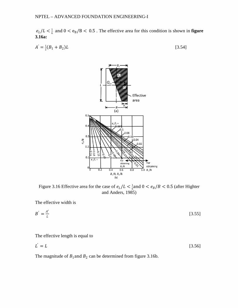
𝑒𝑒𝐿𝐿/𝐿𝐿 < 16 and 0 < eB/B < 0.5 . The effective area for this condition is shown in figure

3.16a:

𝐴𝐴′ = 12(𝐵𝐵1 + 𝐵𝐵2)𝐿𝐿 [3.54]

Figure 3.16 Effective area for the case of 𝑒𝑒𝐿𝐿/𝐿𝐿 < 16and 0 < 𝑒𝑒𝐵𝐵/𝐵𝐵 < 0.5 (after Highter

and Anders, 1985)

The effective width is

𝐵𝐵′ = 𝐴𝐴′𝐿𝐿

[3.55]

The effective length is equal to

𝐿𝐿′ = 𝐿𝐿 [3.56]

The magnitude of 𝐵𝐵1and 𝐵𝐵2 can be determined from figure 3.16b.


Case IV

𝑒𝑒𝐿𝐿/𝐿𝐿 < 16 and eB/B < 1

6. Figure 3.17a shows the effective area for this case. The ratio 𝐵𝐵2/𝐵𝐵 and thus 𝐵𝐵2 can be determined by using the 𝑒𝑒𝐿𝐿/𝐿𝐿 curves that slope upward. Similarly, the ratio 𝐿𝐿2/𝐿𝐿 and thus 𝐿𝐿2 can be determined by using the 𝑒𝑒𝐿𝐿/𝐿𝐿 curves that slope downward. The effective area is then

Figure 3.17 Effective area for the case of 𝑒𝑒𝐿𝐿/𝐿𝐿 < 16and 0 < 𝑒𝑒𝐵𝐵/𝐵𝐵 < 1

6(after Highter and Anders, 1985)

𝐴𝐴′ = 𝐿𝐿2𝐵𝐵 + 12(𝐵𝐵 + 𝐵𝐵2)(𝐿𝐿 − 𝐿𝐿2) [3.57]

The effective width is

𝐵𝐵′ = 𝐴𝐴′𝐿𝐿

[3.58]

The effective length is

𝐿𝐿′ = 𝐿𝐿 [3.59]


Example 6

A square foundation is shown in figure 3.18. Assume that the one-way load eccentricity𝑒𝑒 = 0.15 m. Determine the ultimate load, 𝑄𝑄ult .

Figure 3.18

Solution

With 𝑐𝑐 = 0, equation (43) becomes

𝑞𝑞′𝑢𝑢 = 𝑐𝑐𝑁𝑁𝑞𝑞𝐹𝐹𝑞𝑞𝑐𝑐𝐹𝐹𝑞𝑞𝑐𝑐𝐹𝐹𝑞𝑞𝑒𝑒 + 12𝛾𝛾𝐵𝐵′𝑁𝑁𝛾𝛾𝐹𝐹𝛾𝛾𝑐𝑐𝐹𝐹𝛾𝛾𝑐𝑐𝐹𝐹𝛾𝛾𝑒𝑒

𝑞𝑞 = (0.7)(18) = 12.6 kN/m2

For 𝜙𝜙 = 30°, from table 4, 𝑁𝑁𝑞𝑞 = 18.4 and 𝑁𝑁𝛾𝛾 = 22.4

𝐵𝐵′ = 1.5 − 2(0.15) = 1.2 m

𝐿𝐿′ = 1.5 m

From table 5

𝐹𝐹𝑞𝑞𝑐𝑐 = 1 + 𝐵𝐵′𝐿𝐿′

tan𝜙𝜙 = 1 + �1.21.5� tan 30° = 1.462


= 1 + (0.289)(0.7)1.5

= 1.135


𝐹𝐹𝛾𝛾𝑐𝑐 = 1 − 0.4 �𝐵𝐵′𝐿𝐿′� = 1 − 0.4 �1.2

1.5� = 0.68


So

𝑞𝑞′𝑢𝑢 = (12.6)(18.4)(1.462)(1.135) + 12(18)(1.2)(22.4)(0.68)(1) = 384.7 + 164.50 =

549.2 kN/m2

Hence

𝑄𝑄ult = 𝐵𝐵′𝐿𝐿′�𝑞𝑞′𝑢𝑢� = (1.2)(1.5)(549.2) ≈ 988kN

Example 7

Refer to example 6. Other quantities remaining the same, assume that the load has a two-way eccentricity. Given: 𝑒𝑒𝐿𝐿 = 0.3 m, and 𝑒𝑒𝐵𝐵 = 0.15 m (figure 3.19). Determine the ultimate load, 𝑄𝑄ult .

Figure 3.19

Solution

𝑒𝑒𝐿𝐿𝐿𝐿

= 0.31.5

= 0.2

𝑒𝑒𝐵𝐵𝐵𝐵

= 0.151.5

= 0.1

This case is similar to that shown in figure 3.15a. From figure 3.15b, for 𝑒𝑒𝐿𝐿/𝐿𝐿 =0.2 and eB /B = 0.1

𝐿𝐿1𝐿𝐿≈ 0.85; 𝐿𝐿1 = (0.85)(1.5) = 1.275 m


And

𝐿𝐿2𝐿𝐿≈ 0.21; 𝐿𝐿2 = (0.21)(1.5) = 1.315 m

From equation (51)

𝐴𝐴′ = 12(𝐿𝐿1 + 𝐿𝐿2)𝐵𝐵 = 1

2(1.275 + 0.315)(1.5) = 1.193 m2

From equation (53)

𝐿𝐿′ = 𝐿𝐿1 = 1.275 m

From equation (52)

𝐵𝐵′ = 𝐴𝐴′𝐿𝐿′

= 1.1931.275

= 0.936 m

Note, from equation (43) for 𝑐𝑐 = 0

𝑞𝑞′𝑢𝑢 = 𝑐𝑐𝑁𝑁𝑞𝑞𝐹𝐹𝑞𝑞𝑐𝑐𝐹𝐹𝑞𝑞𝑐𝑐𝐹𝐹𝑞𝑞𝑒𝑒 + 12𝛾𝛾𝐵𝐵′𝑁𝑁𝛾𝛾𝐹𝐹𝛾𝛾𝑐𝑐𝐹𝐹𝛾𝛾𝑐𝑐𝐹𝐹𝛾𝛾𝑒𝑒

𝑞𝑞 = (0.7)(18) = 12.6 kN/m2

For 𝜙𝜙 = 30°, from table 4, 𝑁𝑁𝑞𝑞 = 18.4 and 𝑁𝑁𝛾𝛾 = 22.4. Thus

𝐹𝐹𝑞𝑞𝑐𝑐 = 1 + �𝐵𝐵′𝐿𝐿′� tan𝜙𝜙 = 1 + �1.936

1.275� tan 30° = 1.424

𝐹𝐹𝑞𝑞𝑐𝑐 = 1 − 0.4 �𝐵𝐵′𝐿𝐿′� = 1 − 0.4 �1.936

1.275� = 0.706


= 1 + (0.289)(0.7)1.5

= 1.135


So

𝑞𝑞ult = 𝐴𝐴′𝑞𝑞′𝑢𝑢 = 𝐴𝐴′(𝑞𝑞𝑁𝑁𝑞𝑞𝐹𝐹𝑞𝑞𝑐𝑐𝐹𝐹𝑞𝑞𝑐𝑐 + 12𝛾𝛾𝐵𝐵

′𝑁𝑁𝛾𝛾𝐹𝐹𝛾𝛾𝑐𝑐𝐹𝐹𝛾𝛾𝑐𝑐 =(1.193)[(12.6)(18.4)(1.424)(1.135) + (0.5)(18)(0.936)(22.4)(0.706)(1)] =605.95 kN

Topics - NPTELnptel.ac.in/courses/105104137/module3/lecture10.pdf · Topics 1.1 THE GENERAL ... a...

Documents

Transcript of Topics - NPTELnptel.ac.in/courses/105104137/module3/lecture10.pdf · Topics 1.1 THE GENERAL ... a...