Topics in Two-Dimensional Analytic Geometry -...
26
Chapter 12 Topics in Two-Dimensional Analytic Geometry In this chapter we look at topics in analytic geometry so we can use our calculus in many new settings. Most of the discussion will involve developing these settings, but once developed we will have some immediate input from our calculus. Analytic geometry is the name we give to the combining of geometry with theories of equa- tions. For instance, we place xy-coordinate axes in a plane, renaming the plane Euclidean or Cartesian 2-space, and immediately we can associate every line with an equations Ax + By = C for some A,B,C ∈ R. Thus we can associate geometric figures with equations involving x and y, and vice-versa, which opens up the possibility of algebraic and calculus-based analysis of ge- ometric figures, and geometric analysis of the equations. It is nearly impossible to exaggerate the importance of these connections between equations and geometric objects. We will not always use x and y, also known as rectangular coordinates, to describe points and equations. In particular, we will be interested in polar coordinates, which have many uses as well. We will also generalize the idea of a position (x, y) to the idea of a vector −−→ PQ. In the next chapter, we will extend these ideas into three-dimensional space, with rectangular coordinates (x, y, z ), as well as cylindrical and spherical coordinates. We will examine lines and planes in space, surfaces in space, three-dimensional vectors and their applications. 810
Transcript of Topics in Two-Dimensional Analytic Geometry -...

Chapter 12
Topics in Two-DimensionalAnalytic Geometry
In this chapter we look at topics in analytic geometry so we can use our calculus in many newsettings. Most of the discussion will involve developing these settings, but once developed wewill have some immediate input from our calculus.
Analytic geometry is the name we give to the combining of geometry with theories of equa-tions. For instance, we place xy-coordinate axes in a plane, renaming the plane Euclidean orCartesian 2-space, and immediately we can associate every line with an equations Ax + By = Cfor some A, B, C ∈ R. Thus we can associate geometric figures with equations involving x andy, and vice-versa, which opens up the possibility of algebraic and calculus-based analysis of ge-ometric figures, and geometric analysis of the equations. It is nearly impossible to exaggeratethe importance of these connections between equations and geometric objects.
We will not always use x and y, also known as rectangular coordinates, to describe pointsand equations. In particular, we will be interested in polar coordinates, which have many uses
as well. We will also generalize the idea of a position (x, y) to the idea of a vector−−→PQ.
In the next chapter, we will extend these ideas into three-dimensional space, with rectangularcoordinates (x, y, z), as well as cylindrical and spherical coordinates. We will examine lines andplanes in space, surfaces in space, three-dimensional vectors and their applications.
810

12.1. CONIC SECTIONS 811
Figure 12.1: Congruent infinite right-circular cones (with the same axes of symmetry andvertices), with intersecting planes. The plane will intersect the cones in either a single point, aline, two lines or a conic section: i.e., a parabola, a circle, an ellipse, or a hyperbola. Graphicis from Wikimedia Commons.
12.1 Conic Sections
In short, conic sections are plane curves which are either circles, ellipses, parabolas or hyperbolas.By their natures, there are multiple ways of approaching these curves. We will only consider thosewith vertical or horizontal lines of symmetry.1 We will first look at the actually definitions of theconic sections, but these are only occasionally necessary in applications, particularly in opticsand astronomy, so we will then look at how to draw their graphs based upon their equationswithout referencing their definitions. Finally we will see how the definitions give rise to theequations, which will help us to write the equations given different types of data for the curves,including the location of foci.
12.1.1 Conic Sections Defined Geometrically
A conic section is an intersection of a single plane with two stacked, congruent, infinite rightcircular cones. This is illustrated in Figure 12.1. From there we can see that there are severalways these geometric figures can intersect. Not included in the Figure 12.1 above are otherpossibilities, which are not of interest here except as “degenerate cases,” such as a single point, asingle line or two lines meeting at the vertices of the cones (left to the imagination of the reader).The more interesting cases we deal with here are the parabola, ellipse (including the circle), andthe hyperbola. When one uses the term “conic section,” it is usually in reference to these “moreinteresting” cases.
However, there are other definitions of these figures, based upon distances. The circle is theeasiest: the set of all points in a plane which are the same, fixed distance, or radius from a fixedpoint, called the center, also in the plane. If the center is (h, k) and the radius is r, this definitionquickly becomes (from the Pythagorean Theorem)
√
(x − h)2 + (y − k)2 = r,
1A dedicated analytic geometry or a linear algebra course can be appropriate settings to consider equationsof rotated conic sections with non-vertical or non-horizontal lines of symmetry.

812 CHAPTER 12. TOPICS IN TWO-DIMENSIONAL ANALYTIC GEOMETRY
or the more common form, which is equivalent since r > 0:
(x − h)2 + (y − k)2 = r2. (12.1)
For r = 0 our “circle” would be a single point, which is also a possible intersection of a planewith our cones above. Thus one can debate whether or not to consider a single point to somehowbe a circle.
The ellipse is defined somewhat similarly, except that for the ellipse we take two fixed points,or foci (singular is “focus”) in the plane, and find all points whose distances sum to some fixedtotal distance. A special case of this can be seen in Figure 12.6, page 822. It will take someeffort to derive the form of an equation for an ellipse from this definition, and we will do so later,in Subsection 12.1.3.
Next in complexity is the parabola, which is defined by all the points in the plane whosedistance to a fixed point, or focus in the plane, is the same as the distance to a fixed line, ordirectrix lying in the plane but not containing the focus. This is illustrated in Figure 12.5,page 821. The derivation of an equation for a parabola is somewhat simpler, and will also beincluded later.
Finally, there is the hyperbola, which is defined by all points in a plane whose distances totwo fixed points, or foci in the plane, differ (in absolute value) by a constant. This is illustratedin Figure 12.7, page 824.
While the definitions are interesting and illustrative, we can do much with these figureswithout resorting to these definitions, or even the foci or (in the case of the parabola) directrixes(also called directrices). This is because we can get much general information regarding thepositions and shapes of the figures from simplified equations in which a focus or directrix doesnot appear directly. For completeness we will return to these definitions in Subsection 12.1.3,and use information from those derivations in later computations. While we can draw, say, aparabola without knowing its focus or directrix, if we are interested in optics or acoustics thesethings are more important. For most calculus applications they are not so much.
12.1.2 Simplest Equations of Conic Sections
Most algebra students learn quickly that the graph of y = x2 is a parabola.2 After plottingsimple points, we see a line of symmetry x = 0, intersecting at a vertex (0, 0). After a smallamount of the graphical theory of functions, one usually then learns that any equation of theform
f(x) = a(x − h)2 + k, a 6= 0 (12.2)
will be similar, but with the vertex shifted to (h, k), the axis of symmetry now being x = h, andthe parabola opening upward if a > 0, and downward if a < 0. Shortly after that, one is taughtthat any function of the form f(x) = ax2 + bx + c (a 6= 0) is also a parabola, and we can use
2However, many algebra students make the mistake of believing that any “U-shaped,” or upside-down U-shaped curve is a parabola. Just as not every round “loop”is a circle, we should not expect every curve whoseshape superficially resembles a parabola to actually be a parabola. The curve y = sinx, for x ∈ [0, π] is onesuch example, which resembles a parabola but is in fact not a piece of a parabola. Nor are either branches of ahyperbola “parabolic.” Similarly, not every “oval” is an ellipse.
12.1. CONIC SECTIONS 813
completing the square to find its form (12.2):3
f(x) = ax2 + bx + c
= a
(
x2 +b
ax
)
+ c
= a
[
x2 +b
ax +
(b
2a
)2
−(
b
2a
)2]
+ c
= a
(
x − b
2a
)2
− a · b2
4a2+ c
= a
(
x − b
2a
)2
+
(
c − b2
4a
)
.
Thus y = f(x) has the same shape as y = ax2 except it has been moved horizontally by h = b2a
and vertically by k = c − b2
4a.
Example 12.1.1 Find the vertex and graph the parabola y = 3x2 + 18x − 2.Solution: We do as above, completing the square after first factoring the second and first-
degree terms collectively. Recall that when completing a square of the form x2 + βx, we add
and subtract (β/2)2, to get x2 + βx + β2/4 − β2/4 =(
x + β2
)2
− β2/4.
y = 3(x2 + 6x) − 2 = 3(x2 + 6x + 9︸ ︷︷ ︸
perfect square
−9) − 2
= 3(x + 3)2 − 27 − 2 = 3(x + 3)2 − 29.
Thus we are asked to plot y = 3(x + 3)2 − 29, which has a vertex at (−3,−29). It is commonpractice to plot the vertex and two symmetric points, such as x = h± 1 if it is convenient. Herethat would be the points (−2,−26) and (−4,−26). Because of the location of the curve, we omitthe axes here:
(−2,−26)(−4,−26)
(−3,−29)
Of course there are also those of the form
x = a(y − k)2 + h, or x − h = a(y − k)2.
3Since we have calculus here we can certainly use it to find that the one critical point where f ′(x) = 0 is atx = −b/2a, and that this must be the vertex of the parabola.

814 CHAPTER 12. TOPICS IN TWO-DIMENSIONAL ANALYTIC GEOMETRY
These open horizontally, to the right (vertex on the left) if a > 0, and to the left if a < 0.Now consider an equation which is claimed to represent an ellipse:
Example 12.1.2 Consider the curvex2
9+
y2
16= 1.
Note that this is a variation on the unit circle x2 +y2 = 1, except for scaling in the horizontaland vertical directions. In fact the above equation can be rewritten
(x
3
)2
+(y
4
)2
= 1.
If we look at ordered pairs (X, Y ) which satisfy x2 + y2 = 1, then for analogous points on theellipse (x/3)2 + (y/4)2 = 1 we require (3X, 4Y ):
(3X/3)2 + (4Y/4)2 = 1 ⇐⇒ X2 + Y 2 = 1.
This effectively stretches the graph by a factor of 3 in the horizontal direction, and by a factorof 4 in the vertical direction, giving us our ellipse. Below we give the graphs, equations, and oneanalogous point on each.
x2 + y2 = 1
Example: (x, y) = (1/2,√
3/2)
(1/2)2 + (√
3/2)2 = 1(x/3)2 + (y/4)2 = 1
Example: (x, y) = (3/2, 4√
3/2)
((3/2)/3)2 + ((4√
3/2)/4)2 = 1
1
4
3
x 7−→ (x/3)
y 7−→ (y/4)
The example above, properly generalized, indicates a method of efficient plotting of ellipses.If we generalize this to have different centers (h, k) (not simply (0, 0) as above), we get a form
(x − h)2
a2+
(y − k)2
b2= 1. (12.3)
Here we assume a, b > 0. For any such equation, graphing the ellipse is straight-forward:� Identify the center (h, k), and label it.� From the center, move left and right by a to find the points along the horizontal axis.� From the center, move up and down by b to find the points on the vertical axis.� Graph the ellipse.

12.1. CONIC SECTIONS 815
(h, k)
(h, k − b)
(h, k + b)
(h + a, k)(h − a, k)aa
b
b
(h, k)
(h, k − b)
(h, k + b)
(h + a, k)(h − a, k)aa
b
b
Figure 12.2: Ellipses with equations (x − h)2/a2 + (y − k)2/b2 = 1. The centers are (h, k)in both cases. For the first ellipse, a < b, so it has a vertical major axis of length 2a, andhorizontal minor axis of length 2b. In the second ellipse, a > b so the major axis is horizontalwith length 2a, and the minor axis is vertical with length 2b.
See Figure 12.2. There we see two axes: a horizontal axis of length 2a, and a vertical axis oflength 2b. The longer of these axes is called the major axis, and the shorter of these axes iscalled the minor axis.
Example 12.1.3 Consider the ellipse(x + 2)2
9+
(y − 3)2
16= 1. The center is (−2, 3), and a = 3,
b = 4, so four points we can plot immediately are (−2 ± 3, 3), (−2, 3 ± 4), i.e, points (−5, 3),(1, 3), (−2,−1) and (−2, 7):
3
4
On occasion, some algebraic manipulations are required to get the form (12.3).
Example 12.1.4 Find the center and four axis (major and minor) points of the ellipse
4x2 − 12x + 5y2 + 20y = 0.

816 CHAPTER 12. TOPICS IN TWO-DIMENSIONAL ANALYTIC GEOMETRY
Solution: The usual process of completing the square, and the final steps to have the constant1 on the right-hand side, are as follow:
4x2 − 12x + 5y2 + 20y = 0
⇐⇒ 4(x2 − 3x) + 5(y2 + 4y) = 0
⇐⇒ 4
(
x2 − 3x +9
4− 9
4
)
+ 5(y2 + 4y + 4 − 4) = 0
⇐⇒ 4(x − 3/2)2 − 9 + 5(y + 2)2 − 20 = 0
⇐⇒ 4(x − 3/2)2 + 5(y + 2)2 = 29
⇐⇒ 4
29(x − 3/2)2 +
5
29(y + 2)2 = 1
⇐⇒ (x − 3/2)2
29/4+
(y + 2)2
29/5= 1.
From this we see the center is (3/2,−2), and the points on the axes are
(
3
2±
√29
2,−2
)
,
(
3
2,−2 ±
√
29
5
)
.
More useful for graphing perhaps are decimal approximations of these points:
(4.19,−2), (−1.19,−2), (1.5, .41), (1.5,−4.4).
A rough sketch of this ellipse is then relatively easy, either by plotting the four points above, orby using the distances a = 1
2
√29 ≈ 2.69, and b =
√
29/5 ≈ 2.41. Since these are so similar inlength, the ellipse is closer to “circular” than the previous examples.
1 2 3 4−1
−1
−2
−3
−4
1
2
√29 ≈ 2.69
√
29/5≈
2.4
1
For the hyperbola, we start with the simplest examples, namely x2− y2 = 1 and y2−x2 = 1.These are illustrated in Figure 12.3 Let us take these in turn, though we note that there is aclear analogy between the two curves, as x and y basically exchange roles.� x2 − y2 = 1: For this curve, we first note that x2 = 1 − y2 ∈ [1,∞, which requires
|x| ∈ [1,∞), i.e., x ∈ (−∞,−1] ∪ [1,∞). Therefore x is somewhat limited in possiblevalues, while y is not. In fact the “vertices” of the hyperbola will occur where x = ±1,
12.1. CONIC SECTIONS 817
1 2 3 4−1−2−3−4
1
2
3
4
−1
−2
−3
−4
x2 − y2 = 1
1 2 3 4−1−2−3−4
1
2
3
4
−1
−2
−3
−4
y2 − x2 = 1
Figure 12.3: Illustrations of the simplest hyperbolas considered here: x2 − y2 = 1 andy2 − x2 = 1. In both cases, for large x we have y ≈ ±x, giving us two linear asymptotes.
and y = 0. From the equation, the graph is obviously symmetric with respect to bothaxes, since (a, b) on the graph means all possible combinations of (±a,±b) will also be onthe graph. The line of symmetry passing through both vertices is called the axis of thehyperbola, which in this case is the x-axis. Finally, for large x we have
y = ±√
x2 + 1 ≈ ±√
x2 = ±|x| = ±x,
giving us the two asymptotic lines y = x and y = −x.� y2−x2 = 1: For this curve, we require y ∈ (−∞,−1]∪ [1,∞), but there is no restriction onx. The vertices occur where y = ±1, and x = 0, and the graph is symmetric with respectto both axes, the y-axis being the axis of this particular hyperbola. Finally, for large x wehave
y = ±√
x2 + 1 ≈ ±√
x2 = ±|x| = ±x,
again giving us asymptotic lines y = x and y = −x.
Note that both hyperbolas have a natural “center” at (0, 0), which is both where the asymp-totes intersect each other, and a point with respect to which the parabola is symmetric (in the“inverting lens” fashion).
We can now find our general equation of the hyperbola centered at (h, k):
(x − h)2
a2− (y − k)2
b2= 1, (12.4)
(y − h)2
b2− (x − h)2
a2= 1. (12.5)
For the case (12.4), the vertices are at (h± a, k), and the axis is the line y = k. For case (12.5),the vertices are at (h, k ± b), and the axis is the line x = h. In both cases, we have center (h, k),asymptotes through (h, k) with slopes m = ± b
a:
y − k ≈ ± b
a(x − h). (12.6)
In fact, when graphing these it is simpler to use the point (h, k) and the slopes ±b/a, ratherthan using (12.6).
818 CHAPTER 12. TOPICS IN TWO-DIMENSIONAL ANALYTIC GEOMETRY
1 2 3 4 5 6 7−1−2−3−4−5
1
2
3
4
5
−1
−2
−3
−4
−5
−6
−7
33
4
4(x−2)2
9− (y+1)2
16= 1 :
(y+1)2
16− (x−2)2
9= 1 :
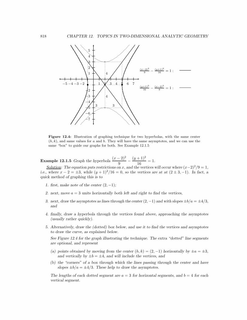
Figure 12.4: Illustration of graphing technique for two hyperbolas, with the same center(h, k), and same values for a and b. They will have the same asymptotes, and we can use thesame “box” to guide our graphs for both. See Example 12.1.5
Example 12.1.5 Graph the hyperbola(x − 2)2
9− (y + 1)2
16= 1.
Solution: The equation puts restrictions on x, and the vertices will occur where (x−2)2/9 = 1,i.e., where x − 2 = ±3, while (y + 1)2/16 = 0, so the vertices are at at (2 ± 3,−1). In fact, aquick method of graphing this is to
1. first, make note of the center (2,−1);
2. next, move a = 3 units horizontally both left and right to find the vertices,
3. next, draw the asymptotes as lines through the center (2,−1) and with slopes ±b/a = ±4/3,and
4. finally, draw a hyperbola through the vertices found above, approaching the asymptotes(usually rather quickly).
5. Alternatively, draw the (dotted) box below, and use it to find the vertices and asymptotesto draw the curve, as explained below.
See Figure 12.4 for the graph illustrating the technique. The extra “dotted” line segmentsare optional, and represent
(a) points obtained by moving from the center (h, k) = (2,−1) horizontally by ±a = ±3,and vertically by ±b = ±4, and will include the vertices, and
(b) the “corners” of a box through which the lines passing through the center and haveslopes ±b/a = ±4/3. These help to draw the asymptotes.
The lengths of each dotted segment are a = 3 for horizontal segments, and b = 4 for eachvertical segment.

12.1. CONIC SECTIONS 819
It should be pointed out that the related hyperbola
(y + 1)2
16− (x − 2)2
9= 1
will have the same asymptotes, and the same “box” as above, though the vertices will be at(h, k ± b) = (−2, 3), (−2,−5). The graph of this hyperbola is superimposed on the graph for thehyperbola in Example 12.1.5, but in dashed, gray lines.
If the equation of the hyperbola is not given in the standard forms (12.4) or (12.5), we mayneed to manipulate the given equation to achieve such form.
Example 12.1.6 Graph the equation 2x2 − 6x = 3y2 − 18y.
Solution: We will complete both squares separately, and see what is left outside the squaresto decide which form the standard equation should have.
2(x2 − 3x) = 3(y2 − 6y)
⇐⇒ 2
(
x2 − 3x +9
4− 9
4
)
= 3(y2 − 6y + 9 − 9)
⇐⇒ 2
(
x − 3
2
)2
− 9
2= 3(y − 3)2 − 27
⇐⇒ 27 − 9
2= 3(y − 3)2 − 2
(
x − 3
2
)2
⇐⇒ 45
2= 3(y − 3)2 − 2
(
x − 3
2
)2
⇐⇒ 1 =3(y − 3)2
45/2− 2
(x − 3
2
)2
45/2
⇐⇒ 1 =(y − 3)2
15/2−(x − 3
2
)2
45/4.
If we wish to make the form more obvious, we could write
(y − 3)2
(√15
2
)2−(x − 3
2
)2
(3√
5
2
)2= 1.
Here, a = 3
2
√5 ≈ 3.3541, and b =
√
15/2 ≈ 2.73861, which will help us to graph the hyperbola
reasonably. Note that the slopes of the asymptotes are ±b/a = ±√
5·32· 2
3√
5=√
2/3 ≈ ±0.81650.
Using the center (3/2, 3) we can graph the hyperbola, though if we sketch it by hand we can use±b/a ≈ ±4/5, for instance (though the graph below is computer-generated).

820 CHAPTER 12. TOPICS IN TWO-DIMENSIONAL ANALYTIC GEOMETRY
1 2 3 4 5 6 7 8 9−1−2−3−4−5−6
1
2
3
4
5
6
7
8
9
10
−1
−2
−3
−4
−1
b
a
a =3
2
√5 ≈ 3.35410,
b =p
15/2 ≈ 2.73861
12.1. CONIC SECTIONS 821
(h, k)
(h, k + p)
y = k − p
(x, y)
(x, k − p)
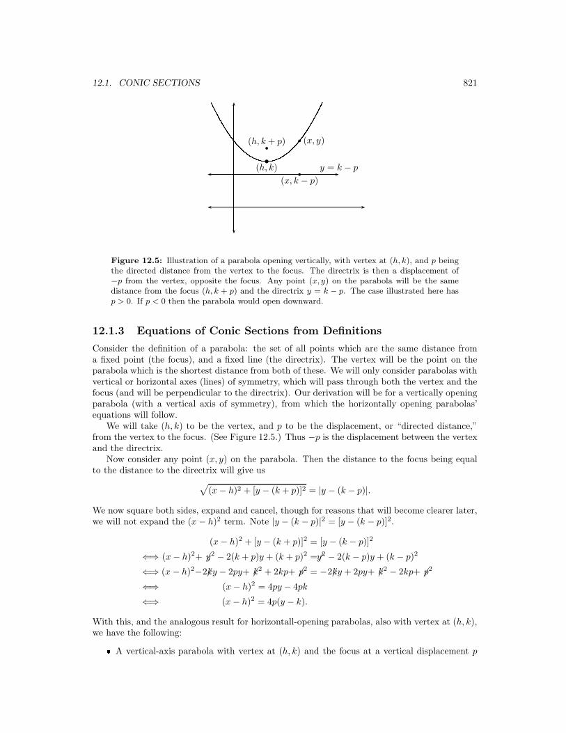
Figure 12.5: Illustration of a parabola opening vertically, with vertex at (h, k), and p beingthe directed distance from the vertex to the focus. The directrix is then a displacement of−p from the vertex, opposite the focus. Any point (x, y) on the parabola will be the samedistance from the focus (h, k + p) and the directrix y = k − p. The case illustrated here hasp > 0. If p < 0 then the parabola would open downward.
12.1.3 Equations of Conic Sections from Definitions
Consider the definition of a parabola: the set of all points which are the same distance froma fixed point (the focus), and a fixed line (the directrix). The vertex will be the point on theparabola which is the shortest distance from both of these. We will only consider parabolas withvertical or horizontal axes (lines) of symmetry, which will pass through both the vertex and thefocus (and will be perpendicular to the directrix). Our derivation will be for a vertically openingparabola (with a vertical axis of symmetry), from which the horizontally opening parabolas’equations will follow.
We will take (h, k) to be the vertex, and p to be the displacement, or “directed distance,”from the vertex to the focus. (See Figure 12.5.) Thus −p is the displacement between the vertexand the directrix.
Now consider any point (x, y) on the parabola. Then the distance to the focus being equalto the distance to the directrix will give us
√
(x − h)2 + [y − (k + p)]2 = |y − (k − p)|.
We now square both sides, expand and cancel, though for reasons that will become clearer later,we will not expand the (x − h)2 term. Note |y − (k − p)|2 = [y − (k − p)]2.
(x − h)2 + [y − (k + p)]2 = [y − (k − p)]2
⇐⇒ (x − h)2+ 6y2 − 2(k + p)y + (k + p)2 = 6y2 − 2(k − p)y + (k − p)2
⇐⇒ (x − h)2− 62ky − 2py+ 6k2 + 2kp+ 6p2 = − 62ky + 2py+ 6k2 − 2kp+ 6p2
⇐⇒ (x − h)2 = 4py − 4pk
⇐⇒ (x − h)2 = 4p(y − k).
With this, and the analogous result for horizontall-opening parabolas, also with vertex at (h, k),we have the following:� A vertical-axis parabola with vertex at (h, k) and the focus at a vertical displacement p

822 CHAPTER 12. TOPICS IN TWO-DIMENSIONAL ANALYTIC GEOMETRY
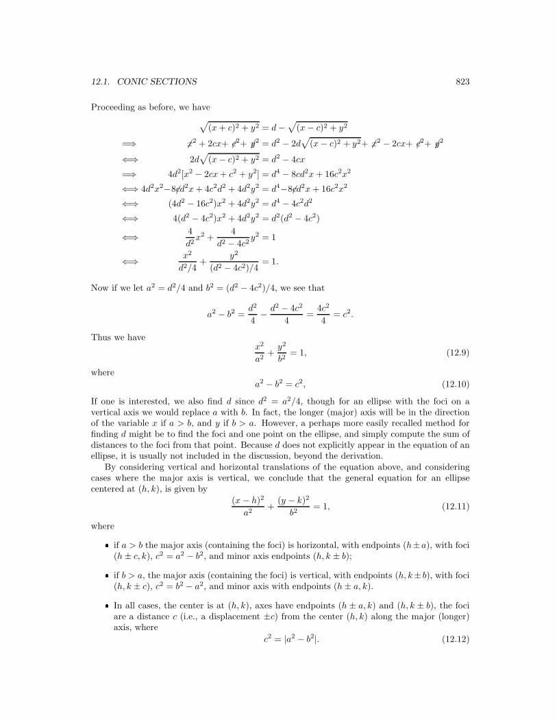
(x, y)
−c c
(0, b)
(0,−b)
(a, 0)(−a, 0)
Figure 12.6: A special case of an ellipse, with foci at (−c, 0) and (c, 0). When we add thedistances from any point (x, y) on the ellipse to the foci, the sum will be constant.
from the vertex will have equation
(x − h)2 = 4p(y − k),
focus = (h, k + p),
directrix: y = k − p.
(12.7)
� A horizontal-axis parabola with vertex at (h, k) and the focus at a horizontal displacementp from the vertex will have equation
(y − k)2 = 4p(x − h),
focus = (h + p, k),
directrix: x = k − p.
(12.8)
For the ellipse, we choose some distance d which is the sum of the distances from a point(x, y) to the foci, which we will assume for simplicity are located at (±c, 0). (We can easillyadjust for more complicated cases later.) If we let d be the sum of distances from (x, y) to thetwo foci, we get
√
(x + c)2 + y2 +√
(x − c)2 + y2 = d.
One needs to square both sides to remove the radicals, but this can not be done in one step.It is usually algebraically simpler to have one of the radicals alone on one side before squaring.
12.1. CONIC SECTIONS 823
Proceeding as before, we have
√
(x + c)2 + y2 = d −√
(x − c)2 + y2
=⇒ 6x2 + 2cx+ 6c2+ 6y2 = d2 − 2d√
(x − c)2 + y2+ 6x2 − 2cx+ 6c2+ 6y2
⇐⇒ 2d√
(x − c)2 + y2 = d2 − 4cx
=⇒ 4d2[x2 − 2cx + c2 + y2] = d4 − 8cd2x + 16c2x2
⇐⇒ 4d2x2− 68cd2x + 4c2d2 + 4d2y2 = d4− 68cd2x + 16c2x2
⇐⇒ (4d2 − 16c2)x2 + 4d2y2 = d4 − 4c2d2
⇐⇒ 4(d2 − 4c2)x2 + 4d2y2 = d2(d2 − 4c2)
⇐⇒ 4
d2x2 +
4
d2 − 4c2y2 = 1
⇐⇒ x2
d2/4+
y2
(d2 − 4c2)/4= 1.
Now if we let a2 = d2/4 and b2 = (d2 − 4c2)/4, we see that
a2 − b2 =d2
4− d2 − 4c2
4=
4c2
4= c2.
Thus we havex2
a2+
y2
b2= 1, (12.9)
where
a2 − b2 = c2, (12.10)
If one is interested, we also find d since d2 = a2/4, though for an ellipse with the foci on avertical axis we would replace a with b. In fact, the longer (major) axis will be in the directionof the variable x if a > b, and y if b > a. However, a perhaps more easily recalled method forfinding d might be to find the foci and one point on the ellipse, and simply compute the sum ofdistances to the foci from that point. Because d does not explicitly appear in the equation of anellipse, it is usually not included in the discussion, beyond the derivation.
By considering vertical and horizontal translations of the equation above, and consideringcases where the major axis is vertical, we conclude that the general equation for an ellipsecentered at (h, k), is given by
(x − h)2
a2+
(y − k)2
b2= 1, (12.11)
where� if a > b the major axis (containing the foci) is horizontal, with endpoints (h±a), with foci(h ± c, k), c2 = a2 − b2, and minor axis endpoints (h, k ± b);� if b > a, the major axis (containing the foci) is vertical, with endpoints (h, k± b), with foci(h, k ± c), c2 = b2 − a2, and minor axis with endpoints (h ± a, k).� In all cases, the center is at (h, k), axes have endpoints (h ± a, k) and (h, k ± b), the fociare a distance c (i.e., a displacement ±c) from the center (h, k) along the major (longer)axis, where
c2 = |a2 − b2|. (12.12)
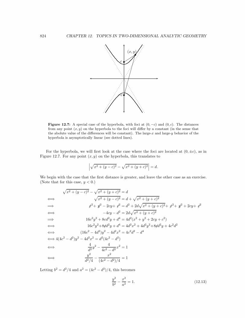
824 CHAPTER 12. TOPICS IN TWO-DIMENSIONAL ANALYTIC GEOMETRY
(x, y)
c
−c
Figure 12.7: A special case of the hyperbola, with foci at (0,−c) and (0, c). The distancesfrom any point (x, y) on the hyperbola to the foci will differ by a constant (in the sense thatthe abolute value of the differences will be constant). The large-x and large-y behavior of thehyperbola is asymptotically linear (see dotted lines).
For the hyperbola, we will first look at the case where the foci are located at (0,±c), as inFigure 12.7. For any point (x, y) on the hyperbola, this translates to
∣∣∣
√
x2 + (y − c)2 −√
x2 + (y + c)2∣∣∣ = d.
We begin with the case that the first distance is greater, and leave the other case as an exercise.(Note that for this case, y < 0.)
√
x2 + (y − c)2 −√
x2 + (y + c)2 = d
⇐⇒√
x2 + (y − c)2 = d +√
x2 + (y + c)2
=⇒ 6x2+ 6y2 − 2cy+ 6c2 = d2 + 2d√
x2 + (y + c)2+ 6x2+ 6y2 + 2cy+ 6c2
⇐⇒ −4cy − d2 = 2d√
x2 + (y + c)2
=⇒ 16c2y2 + 8cd2y + d4 = 4d2(x2 + y2 + 2cy + c2)
⇐⇒ 16c2y2+ 68cd2y + d4 = 4d2x2 + 4d2y2+ 68cd2y + 4c2d2
⇐⇒ (16c2 − 4d2)y2 − 4d2x2 = 4c2d2 − d4
⇐⇒ 4(4c2 − d2)y2 − 4d2x2 = d2(4c2 − d2)
⇐⇒ 4
d2y2 − 4
4c2 − d2x2 = 1
⇐⇒ y2
d2/4− x2
(4c2 − d2)/4= 1
Letting b2 = d2/4 and a2 = (4c2 − d2)/4, this becomes
y2
b2− x2
a2= 1. (12.13)

12.1. CONIC SECTIONS 825
Note that b2 + a2 = 4c2/4, i.e.,
a2 + b2 = c2. (12.14)
Note that if we solve for y in (12.13), we have
y2
b2= 1 +
x2
a2
=⇒ y2 = b2 +b2
a2x2
⇐⇒ y = ± b
a
√
a2 + x2 ≈ ± b
a
√x2,
(12.15)
this last line being for large x. Recall√
x2 = |x| = ±x, depending upon whether x ≥ 0 or x < 0.Thus,
x large =⇒ y ≈ ± b
ax. (12.16)
We see that the large-x behavior is for y ≈ ± bax, which gives two linear asymptotes: y = b
ax
and y = − bax. It is also notable that y2
b2≥ 1 gives us y2 ≥ b2, requiring y ≥ b or y ≤ −b, i.e.,
y ∈ (−∞,−b] ∪ [b,∞), so y is somewhat limited in possible values, where x is not, as we cansee within the equations (12.15). The vertices of the hyperbola are at (0,±b). Through thosevertices is the axis. Of course there are two lines of symmetry, the axis and the line through thecenter (0,0) and perpendicular to the axis.
Looking at translations of our simplified model, we get a general form with translated features.The equation and the hyperbola’s features will be as follow:
(y − k)2
b2− (x − h)2
a2= 1 (12.17)� centered at (h, k),� vertical axis line x = h� asymptotes y − k = ± b
a(x − h), i.e., containing (h, k) with slopes ± b
a,� vertices at (h, k ± b),� foci at vertical distances c from the center (h, k), i.e., at (h, k ± c), where c2 = a2 + b2
If instead we have a horizontal axis, we have:
(x − h)2
a2− (y − k)2
b2= 1 (12.18)� centered at (h, k),� horizontal axis line y = k� asymptotes y − k = ± b
a(x − h), i.e., containing (h, k) with slopes ± b
a,� vertices at (h ± a, k),� foci at vertical distances c from the center (h, k), i.e., at (h ± c, k), where c2 = a2 + b2

826 CHAPTER 12. TOPICS IN TWO-DIMENSIONAL ANALYTIC GEOMETRY
12.1.4 Eccentricity
Physicists often discuss a concept called eccentricity, associated with conic sections or, moreloosely, how much a curved path deviates from a circle (which then has zero eccentricity). Formost of our conic sections, it is the ratio of the distance from the “center” to a focus, dividedby the distance from the center to a vertex. For the ellipse, this would be e = c/a if a > b,or e = c/b if b > a, so we can simply write e = c/ max{a, b}. Since c2 = |a2 − b2|, we havec < max{a, b}, 0 < e < 1 for an ellipse. A circle is like an ellipse with both foci at the center(c = 0), so e = 0. For a hyperbola, c2 = a2 + b2 so e = c/ max{a, b} > 1.
For the parabola, it would seem strange to discuss a “center.” For the other conic sections, itseems that “center” could be the one point through which the conic section is symmetric. Recallthat “symmetric with respect to a point” means that, were that point a “lens,” any part of thefigure on one “side” of the point (“lens”) has a corresponding part which is the optic inversionof the first part through that point (“lens”). However the parabola has no such symmetry withrespect to a point. (For the others, it is at their center (h, k).) The solution is to instead definea “directrix” for each figure, and not just for the parabola, and then the eccentricity is the ratioof the distance from any point on the figure to the focus versus the distance to the directrix.4
From the definition of the parabola—all points which are the same distance to the focus as thedirectrix—we trivially have e = 1.
Exercises
1. Compute the general formula (12.6) forthe asymptotes of a hyperbola for both
(12.4) and (12.5).
4We will not pursue this in depth here, but mention one case here briefly. For an ellipse, the directrix is aline such that the ellipse can be defined as all points (x, y) for which the distance d1 to the focus is proportionalto the perpendicular distance d2 to the directrix. That proportionality constant is then e < 1. For the ellipse inFigure 12.6, a directrix would be x = a2/c, which is to the right of the ellipse since a2/c = a · a
c> a. For the
ellipse below, a = 2, b = 1, so c =√
a2 − b2 =√
3, and then e = c/a =√
3/2 < 1.
1 2 3 4 5−1−2−3
1
−1
d2
d1
d1 = e · d2
= d2 ·√
3/2
≈ 0.8660 · d2
directrix

12.2. PARAMETRIC CURVES 827
12.2 Parametric Curves
The term parametric curve comes from the idea that both the x-coordinate and the y-coordinate of the curve will be functions of a third variable, called the parameter. This allowsfor many more types of curves than those given functionally by y = f(x), and even includessome that would be difficult to give implicitly.
An example of a parametric curve in the plane can be
x = cos t,
y = sin t.
Thus we follow the x-coordinate as t varies, and separately (if we like) the y-coordinate as tvaries. When we graph this for the first time, we might make a chart and graph the points thatoccur, and attempt to deduce the shape of the graph. Choosing t-values with known sines andcosines, we might produce the following table and graph. Note
√3/2 ≈ 0.866, and 1/
√2 ≈ 0.707.
t x = cos t y = sin t0 1 0
π/6√
3/2 1/2
π/4 1/√
2 1/√
2
π/3 1/2√
3/2π/2 0 1
2π/3√
3/2 −1/2
3π/4 1/√
2 −1/√
2
5π/6 1/2 −√
3/2π −1 0
7π/6 −√
3/2 −1/2
5π/4 −1/√
2 −1/√
2
4π/3 −1/2 −√
3/23π/2 0 −1
5π/3 1/2 −√
3/2
7π/4 1/√
2 −1/√
2
11π/6√
3/2 −1/2
1−1
1
−1
t = 0
12.3 Polar Coordinates
12.4 Calculus in Polar Coordinates

828 CHAPTER 12. TOPICS IN TWO-DIMENSIONAL ANALYTIC GEOMETRY
1 2 3 4 5−1−2−3
1
2
3
4
5
−1
−2
−3
〈2,3〉
〈2,3〉
〈2,3〉
〈2,3〉
〈2,3〉
〈2,3〉
〈2,3〉
(2, 3)
〈2,3〉
θ
Figure 12.8: For each vector illustrated above, the displacement from the ”tail” to the ”head”is +2 horizontally, and +3 vertically. Each therefore represent the same (displacement) vector,namely 〈2, 3〉. If we plot the vector 〈2, 3〉 in standard position, i.e., with its tail at the origin(0, 0), we see the head is indeed at (2, 3). The length is ‖ 〈2, 3〉 ‖ =
√13, and the vector points
in the direction θ = tan−1 32, since it is in the first quadrant.
12.5 Vectors in R2; Scalar (Dot) Products
In this section we will look at vectors “in the plane,” particularly the familiar xy-plane, whichis a two-dimensional space.5 Later in the text we will examine vectors in space, also sometimesknown as xyz-space, which is a three-dimensional space.
The classical definition of a vector is a quantity with both magnitude and direction. We willsee that there is an intentional ambiguity in this definition.
Another common defintion of a vector is a directed line segment. This is even more prob-lematic, as it removes exactly the ambiguity that we will see later is crucial to the usefulness ofvectors. Indeed, describing a vector as a directed line segment is a bit like describing an angleas the union of two rays with the same origin. In the former you lose that the crucial elementsare the length and direction (not the geometric position of the vector), while with angles wefind it useful to think of them as rotations of well-defined amounts (and in particular directions)regardless of the pivot points.
Both definitions are somewhat geometric. As with derivatives and definite integrals, thereis a geometric context in which vectors are easily visualized. However, there are other quanti-
5A two-dimensional space is one in which we require two variable to describe a point’s position.

12.5. VECTORS IN R2; SCALAR (DOT) PRODUCTS 829
ties which are “vector quantities,” and there is a purely algebraic definition of a vector whichaccommodates these as well.
To introduce the actual concept of vector, we will use one such example of a vector quantity,which closely mirrors the geometric intuitions. That is the concept of a vector as a displacement.As before, a displacement can be defined to be a net change in position. Suppose for instancewe move from (0, 0) to (2, 3). This would be a change of +2 in the horizontal position, and +3in the vertical.
Now suppose instead we move from (−4,−1) to (−2, 2). This would also be a change of+2 in the horizontal and +3 in the vertical directions, repsectively. Both motions represent thesame net displacement, which we signify by the vector 〈2, 3〉. It does not matter what is ourinitial point, as long as our final point is right 2 and up 3 from our initial point. In all cases itis represented by the same vector 〈2, 3〉. See Figure 12.8 at the beginning of this secction.
While it is important that we realize that each of these displacements—of +2 in the horizontaland +3 in the vertical—is considered to be the same net displacement and therefore the same
vector, for many purposes it is best to define a standard position for vectors, namely that thetail is fixed to the origin (0, 0). Then the head of the vector 〈2, 3〉 would lie at (2, 3).6
The standard position of a vector allows us to easily explain these concepts of magnitudeand direction. The magnitude is a measure of the vector’s size, and the direction is, of course,the direction it points. The length of the vector is given by the notation ‖ 〈2, 3〉 ‖, and thePythagorean Theorem gives it to us immediately: ‖ 〈2, 3〉 ‖ =
√22 + 32 =
√13. More generally,
‖ 〈a, b〉 ‖ =√
a2 + b2. (12.19)
The length of the vector is also known as its magnitude, modulus, and sometimes called itsabsolute value.7 The direction θ in which the vector points is measured off of the positive x-axis,just as is an angle in standard position. In general,
tan θ =a
b, , (12.20)
and does not have to be in any particular range. Some texts will have 0 ≤ θ < 360◦, whileothers will use −180◦ < θ ≤ 180◦, but all that is required is that we allow the angles available todescribe all possible directions in which a vector can point. Note that we usually decline to definea direction for the zero vector 〈0, 0〉, though it clearly has length ‖ 〈0, 0〉 ‖ =
√02 + 02 = 0.
Note also that at the moment we are interested in the geometry of these vectors, not the calculus,so using radian measure for θ is not yet necessary. Some texts defined the argument of the vector,arg〈a, b〉 to be some particular angle θ, but we will usually just describe (albeit more verbosely)the angle in question.
When looking at vectors in the plane, it is only necessary to specify the two coordinates aand b of the endpoints (a, b) where the head of vector 〈a, b〉 points when 〈a, b〉 is in standardposition. Because a, b ∈ R, we often signify the set of all such possible vectors as
R2 =
{
〈a, b〉∣∣∣∣
a, b ∈ R
}
.
Because it takes exactly two numbers to specify to identify the vector, R2 is called a two-
dimensional space.
6This is similar to the “standard position” of an angle θ, which allows much of the analysis—especially of thetrigonometric kind—of such objects.
7When the length of 〈a, b〉 is called its it absolute value, the notation usually reflects this as well: |〈a, b〉| =√a2 + b2.

830 CHAPTER 12. TOPICS IN TWO-DIMENSIONAL ANALYTIC GEOMETRY
1 2 3
1
2
3
−1
〈2,3〉
1 2 3
1
2
3
−1
〈2,3〉
〈2,3〉
Figure 12.9: Two traditional ways to geometrically describe vector addition. Here we illus-trate how these methods predict 〈2, 3〉 + 〈1,−2〉 = 〈3,−1〉.
One of the aspects that makes vectors interesting is how they “add” and similarly combine.It is quite intuitive when put simply, and quite interesting when viewed geometrically. When weadd two vectors in R
2, we do so as follows:
〈a1, b1〉 + 〈a2, b2〉 = 〈a1 + a2, b1 + b2〉.
The new vector is then called the resultant vector, representing the net displacement. As wesee from the equation above, to find the net displacement—when we first displace by 〈a1, b1〉,followed by another displacement of 〈a2, b2〉— we look at the total horizontal displacement a1+a2
and the total vertical displacement b1 + b2 to form our new vector. Algebraically this is verysimple, but at times we will be interested in a geometric perspective. Geometric vector additionis traditionally described in the following two ways:
Tail-to-Head: where the origin (tail) of the second vector is placed at the head of the first;
Parallelogram Rule: where we form a parallelogram with the two vectors, in standard posi-tion, forming one corner, and the resultant vector coming from that corner to the diagonallyopposed corner.

12.5. VECTORS IN R2; SCALAR (DOT) PRODUCTS 831
1 2 3−1−2−3
1
2
3
4
5
6
−1 θ = 11π6
θ = 7π6

832 CHAPTER 12. TOPICS IN TWO-DIMENSIONAL ANALYTIC GEOMETRY
12.6 Three-Dimensional Space
12.7 Vectors in R3; Vector (Cross) Products
12.8 Lines and Planes in R3

12.8. LINES AND PLANES IN R3 833
0 1 2 3 4 5 6 7 8 9 10 11 12 13 140
1
2
3
4
5
6
7
8
9
10
11
12
13
14
15
16
17
18
19
20
Header
Body
Footer
MarginNotes
i8� -
i7
?
6
i1� -
�-i3
i10-�
�-i9
6
?
i11
i2
?
6
6
?
i4
6
?
i5
6
?
i6
1 one inch + \hoffset 2 one inch + \voffset
3 \evensidemargin = 28pt 4 \topmargin = 23pt
5 \headheight = 12pt 6 \headsep = 18pt
7 \textheight = 598pt 8 \textwidth = 417pt
9 \marginparsep = 7pt 10 \marginparwidth = 0pt
11 \footskip = 25pt \marginparpush = 5pt (not shown)
\hoffset = 0pt \voffset = 36pt
\paperwidth = 597pt \paperheight = 845pt

Header
Body
Footer
MarginNotes
i8� -
i7
?
6
i1� -
�-i3
i10-�
�-i9
6
?
i11
i2
?
6
6
?
i4
6
?
i5
6
?
i6
1 one inch + \hoffset 2 one inch + \voffset
3 \oddsidemargin = 28pt 4 \topmargin = 23pt
5 \headheight = 12pt 6 \headsep = 18pt
7 \textheight = 598pt 8 \textwidth = 417pt
9 \marginparsep = 7pt 10 \marginparwidth = 0pt
11 \footskip = 25pt \marginparpush = 5pt (not shown)
\hoffset = 0pt \voffset = 36pt
\paperwidth = 597pt \paperheight = 845pt