REGRESSION TEST SELECTION TO

REDUCE ESCAPED DEFECTS UNDERGRADUATE CONCLUSION WORK

UNIVERSIDADE FEDERAL DE PERNAMBUCO

GRADUAÇÃO EM ENGENHARIA DA COMPUTAÇÃO CENTRO DE INFORMÁTICA

2008.1

Student: Renata Bezerra e Silva de Araújo, rbsa@cin.ufpe.br

Advisor: Augusto César Alves Sampaio, acas@cin.ufpe.br

Co-Advisor: Juliano Manabu Iyoda, jmi@cin.ufpe.br

Recife, June/2008.

2

To my mother: Ubiracema Bezerra.

3

Acknowlegments

I would like to sincerely thank everyone that, somehow, has contributed to

the existence of this work, either helping me directly or simply being part of my life

and making me the person I am today.

First, I want to thank God for being always by my side during this journey,

giving me strength in all moments I needed it.

I am also eternally grateful to my mother, “Cema”, to whom I dedicate this

work. Her support, advices, incentive, talks, jokes and unconditional love have

encouraged me more and more to get here. Mom, I love you so much.

I do thank my family, that I love so much, specially my grandmother, “vó

Maria”, my father Luíz Mário, my brother Fábio, my cousins Heloisa, Maria Zilá and

Márcio, my mother’s husband, Braulio and my brother’s wife, Juliana.

I also want to thank Erick Lopes, for everything that we have lived together,

for all wonderful and unforgotten moments, and of course, for his patience, support

and incentive during my graduation, especially in the moments that I wanted to give

up and he changed my mind with encouragement words.

I really need to thank all my old friends that I love more each day. Special

thanks to “Lidinho”, “Nando”, Príscila, Renata, Sivaldo, “Tati” and Ulisses.

I offer my thanks also for the best friends that I have made during my

academic life. Special thanks to “Aline”, “Grasi”, Luciano, Nitai, and of course,

Thiago Burgo (Thi), my friend since we were teenagers and used to spend our

summer in São José da Coroa Grande.

I cannot forget to thank all the rest of my classroom friends. The ones from

the computer engineering course, that besides sharing a lot of fun and nice moments,

also shared with me the bad moments studying for those difficult disciplines and

doing the projects all night, which was important to make me learn how to deal with

so many difficult moments. My special thanks to “Array”, Bruno, “Cintura”, “Dani”,

“Galeguinho”, “Logan”, Marcus, “Mago”, “Preula”, “Rô”. Also, the ones from the

computer science course, that spent great moments with me too. Thanks to “Bigode”,

4

Cássio, César, “Chico”, “Chicão”, Davi, Ernani, “Farinha”, “Gara”, Hector, Hially,

Igor, ”Mestre”, “Raoni”, “Rubis”, “Sunday”, Vitor.

I do want to thank my friends that have worked with me for almost three

years in Brazil IP. Thanks to Adelmario, Diego, Diogo, Edson, Hudson, Marcelo

Lucena, Renata Garcia, Pyetro and “Seba”.

Finally, I want to thank my masters, especially my advisor, Augusto Sampaio,

for his trust and support, my co-advisor, Juliano Iyoda, for his support, attention and

great help, my supervisor in Brazil IP research, Edna Barros, and Marcília Campos,

my advisor in monitoring the discipline of statistics and probability.

Apologies if I have forgotten someone here, I am not less thankful if it had

happened. For all of you, my sincere thanks, I will be forever grateful. All of you

have inspired me some way.

5

“Live as if you were to die tomorrow. Learn as if you were to live

forever.”

(Mahatma Gandhi)

6

Contents

ACKNOWLEGMENTS ....................................................................................................................... 3

LIST OF FIGURES................................................................................................................................ 7

LIST OF TABLES .................................................................................................................................. 8

ABSTRACT ............................................................................................................................................ 9

RESUMO .............................................................................................................................................. 10

1 INTRODUCTION ..................................................................................................................... 11

1.1 OBJECTIVES .............................................................................................................................. 12

1.2 DOCUMENT STRUCTURE ........................................................................................................... 13

2 SOFTWARE TESTING ............................................................................................................ 14

2.1 RUP TEST DISCIPLINE .............................................................................................................. 15

2.2 ESCAPED DEFECTS ................................................................................................................... 20

2.3 REGRESSION TEST SELECTION ................................................................................................. 21

3 DEBUGGING AND TESTING .............................................................................................. 23

4 TEST SELECTION STRATEGY ............................................................................................. 27

4.1 TEST CASE HISTORY ................................................................................................................ 27

4.2 CHANGED AND NEW COMPONENTS ...................................................................................... 30

4.3 RECENT FAILURES.................................................................................................................... 32

4.4 ESCAPED DEFECTS ................................................................................................................... 34

4.5 SPATIAL LOCALITY .................................................................................................................. 37

5 EXPERIMENTS ......................................................................................................................... 44

5.1 RESULTS ................................................................................................................................... 48

6 CONCLUSION .......................................................................................................................... 51

6.1 RELATED WORK....................................................................................................................... 51

6.2 FUTURE WORKS ....................................................................................................................... 52

REFERENCES ...................................................................................................................................... 53

APPENDIX A – PYTHON CODE FOR THE FIVE METRICS.................................................... 57

7

List of Figures

Figure 1 - The Rational Unified Process ................................................................... 11

Figure 2 – Test discipline workflow ......................................................................... 16

Figure 3 – Test discipline activities ........................................................................... 17

8

List of Tables

Table 1. Agree on the Mission Template .................................................................. 18

Table 2. Activities that compose each workflow detail ............................................. 19

Table 3. Generic structure of Test Case History metric ............................................. 27

Table 4. Generic structure of Changed and New Components metric ........................ 30

Table 5. Generic structure of Recent Failures metric ................................................. 32

Table 6. Example for the Recent Failures metric ...................................................... 33

Table 7. Generic structure of Escaped Defects metric ............................................... 34

Table 8. Example for the Escaped Defects metric ..................................................... 35

Table 9. Generic structure of Spatial Locality metric ................................................ 37

Table 10. Distances .................................................................................................. 40

Table 11. Averages of every c’’ � C’’ and the associated test cases .......................... 40

Table 12. Example for the Spatial Locality metric .................................................... 41

Table 13. Hypothetic data for test case histories ....................................................... 44

Table 14. Hypothetic data for Components visited by each test case ......................... 45

Table 15. Hypothetic data for changed and new components .................................... 46

Table 16. Hypothetic data for failed components ...................................................... 46

Table 17. Hypothetic data for remaining components ............................................... 46

Table 18. Hypothetic data for the percentage of CRs opened for the failed components

......................................................................................................................... 47

Table 19. Hypothetic data for the components that presented escaped defect ............ 47

Table 20. Hypothetic data for the percentages of CRs opened for escaped defects

components ...................................................................................................... 47

Table 21. Hypothetic data for the test cases not performed ....................................... 47

Table 22. Hypothetic data for the history of versions ................................................ 48

Table 23. The results of all metrics ........................................................................... 49

9

Abstract

Software development encompasses an extreme competitive market.

Given that the system quality is an important factor to guarantee the company

position in the market, great effort has been dedicated to ensure the product

quality and customer satisfaction. Due to the enormous possibility of injecting

human failures and its associated costs, a really careful and well planned

testing process is definitely necessary. The main role of software testing is to

find defects in the product so that the development team can fix them on time,

before the product reaches the customer. In this context, the concept of escaped

defects emerges. An escaped defect is a defect that was not found by the test

team in a specific step of the process. As the companies need to keep their

deadlines, when a new build (version) of the product is released it becomes

impracticable the re-execution of all test cases in order to reduce the escaped

defects. Because of that, there are teams responsible for selecting manually a

subset of all test cases to guarantee the software correctness and reduce the

escaped defects. This work focuses on the definition of five criteria (metrics)

that permit a more systematic test case selection from a suite in order to

increase the probability of finding bugs and, hopefully, reduce the number of

defects to escape. This work is done as part of the research project

collaboration between CIn-UFPE and Motorola, in the context of Brazil Test

Center (BTC).

Keywords: Software Testing, Regression Test Selection, Escaped Defects

10

Resumo

O desenvolvimento de software engloba um mercado de extrema

competitividade. Tendo em vista que os sistemas que apresentam melhor

qualidade garantem seu espaço no mercado, as empresas que os desenvolvem

têm investido bastante esforço para assegurar a qualidade do produto e a

satisfação do cliente. Devido à grande possibilidade de injeção de falhas

humanas e dos custos associados a estas falhas, um processo de testes

bastante cuidadoso e bem planejado se faz necessário. O principal objetivo

dos testes de software é encontrar defeitos no produto final, para que a equipe

de desenvolvimento os corrija a tempo, antes que o produto chegue ao cliente.

Dentro deste contexto, surge o conceito de escaped defects (defeitos escapados),

que nada mais são do que defeitos que não foram encontrados pelo time de

teste, em uma etapa específica do processo. Devido à necessidade das

empresas cumprirem seus prazos, quando uma nova build (versão) é liberada,

torna-se inviável a re-execução de todos os testes para diminuir a quantidade

de defeitos escapados. Por isso, geralmente existem equipes responsáveis por

selecionar manualmente um grupo mínimo de casos de teste que sejam

capazes de garantir o correto funcionamento do software. Este trabalho dá

enfoque na definição de cinco critérios (métricas) que permitam uma seleção

mais sistemática dos casos de teste de uma suíte, de modo que esta seleção

aumente as chances de se encontrar defeitos e, possivelmente, reduza a

quantidade de defeitos que escapem. Este trabalho é parte do projeto de

pesquisa do CIn-UFPE em cooperação com a Motorola no contexto do Brazil

Test Center (BTC).

Palavras Chaves: Teste de Software, Seleção de testes de regressão, escaped

defects.

11

1 Introduction

Software development encompasses an extreme competitive market. Given

that the system quality is an important fact to guarantee the company position in the

market, great effort has been dedicated to ensure the product quality and customer

satisfaction.

To ensure product quality, software engineering processes like RUP (Rational

Unified Process®) [1] are often used during the product development, also aiming at

higher productivity. Figure 1 shows an overview of the RUP. It has two dimensions:

the horizontal axis represents time and shows the lifecycle aspects of the process, and

the vertical axis represents disciplines, which group activities logically according to

their nature.

Figure 1 - The Rational Unified Process

The horizontal axis represents the dynamic aspect of the process, i.e. how

activities are distributed over time. It is expressed in terms of Phases and Milestones.

The vertical axis represents the structural aspects of the process: how it is described

in terms of disciplines, workflows, activities, artefacts and roles. Figure 1 also shows

how the emphasis on one activity can vary over time.

Nowadays, a discipline that has shown great importance is the Test discipline,

which this work focuses on. Due to the enormous possibility of injecting human

12

failures in the products and its associated costs, a really careful and well planned

testing process is definitely necessary.

The main role of software testing [4], [5] is to find defects in the product, so

that the development team can fix them on time before the product reaches the

customer. This might be done by verifying whether all requirements are

implemented according to their specification, and also by producing test cases that

present high probability of revealing a fault that was not identified yet, with a

minimum amount of time and effort.

Knowing that problems exposed to customers are quite costly, it is necessary to

develop preventive solutions by creating effective tests that aim to find as many

errors as possible. In this context, the concept of escaped defects [3] emerges. An

escaped defect is a defect that was not found by the test team, in a specific step of the

process.

A research and development project that emerged from a partnership between

CIn-UFPE and Motorola, located in Recife, as part of the Brazil Test Center (BTC)

project, is responsible for conducting tests of the Motorola cell phones with focus on

the software testing execution activities.

In this particular context, defects that are classified as escaped defects are the

ones which were not found by the BTC, appearing in a later phase, say, at system

testing or even in the user hands. The problem characterized as escaped defects [3] may

be addressed by using the idea of Regression Test Selection [6] [7], but, all of the

researches existent in the literature assume availability of the source code. As this is

not the case for the BTC, we have to look at black-box bug prediction techniques to

define our own strategy for regression test selection.

1.1 Objectives

Due to the needs of big companies, like Motorola, to meet their deadlines,

when a new build of a product is released, it becomes impractical the re-execution of

all test cases. Because of that, there are teams responsible for selecting manually a

group of test cases that could be able to guarantee the software correct operation.

13

Within the presented context and based on the Motorola needs of identifying

errors more efficiently, this work aims to propose a solution that allows a more

systematic test cases selection from a suite, so that this selection might allow the

reduction of possible defects to escape.

Particularly, this work is focused on the definition of criteria (metrics)

responsible for promoting a test case selection that will be used to the regression

tests, when a new build (version) is already available. Based on a particular intention

for each criterion, each of them provides a different relevance order among the tests

existent in the suite. The team manager can then compare the results of each criterion

and select the test cases based on the needs of each particular build, giving more

emphasis to the criteria that seem to be the most important.

1.2 Document Structure

This work is organized as follows:

• Chapter 2 presents a detailed description of software testing, focusing

on the RUP test discipline, and also explaining the concepts of escaped

defects and regression test selection, used in this work;

• Chapter 3 explains the concepts of debugging and testing, and shows

how strategies for debugging can be used in software testing;

• Chapter 4 describes the regression test selection strategy proposed; it

describes each of the defined criteria in detail, also presenting a formal

specification for them;

• Chapter 5 introduces the experiments performed in order to illustrate

the strategy proposed;

• Chapter 6 shows the conclusion of this research, also presenting the

related and future works.

14

2 Software Testing

Software testing is “any activity aimed at evaluating an attribute or capability

of a program or system and determining that it meets its required results” [8].

In a simple way, one of the main purposes of software testing is to execute a

developed system in order to find bugs. This contrasts with the other purpose of

testing: to ensure that the system does what it is suppose to do.

Software testing is therefore important to analyse whether the implementation

meets the system requirements, to reduce the costs associated to maintenance and re-

work, to verify the correct integration among all software components, and

especially, to ensure the client satisfaction.

The idea of finding bugs has the intent of reporting them back to the

development team, so they can fix them. In this way, the final product shall have as

few bugs as possible, guaranteeing its quality and reliability. It is impossible to find

all bugs existent in a program with testing, so it is important to know that software

will always have bugs. Then, the objective is to provide systems in which the

remaining bugs are neither critical nor essential and which do not compromise the

system integrity.

There are two main testing approaches: white box and black box. The former is

characterized by knowing the internal functionalities of the software components; so

it is necessary to have programming skills to understand all possible logical paths.

On the other hand, differently from the white box approach, the latter approach

regards software as a black box, where its internal structure is not considered. Given

the input data, its aim is to verify whether the given outputs are as expected.

The moments in the software life cycle in which tests are performed can be

defined by four test phases: Unit testing, Integration testing, System testing and,

finally, Acceptance testing [9]. Unit testing is the act of testing isolated components,

ensuring their individual correctness in order to make much easier the Integration

testing, which is responsible to test the integration among the unit parts. System

testing verifies the whole system functionality, and in general, black box tests are

15

executed with this intention. Finally, the system is tested by the user in order to

approve it (Acceptance testing).

When changes are made to the software, a new build is released, and

regression tests must be performed. They are responsible to verify whether

previously-working functionality did not regress and to verify whether the changes

are working as expected.

2.1 RUP Test Discipline

As shown in Figure 1 of Chapter 1 the RUP Test discipline already begins in

the Inception phase, during project planning. Here, the initial planning of the tests is

done based on the project plan and also on the elicited requirements, which are one

of the first inputs for identifying which tests to perform. In the next phase –

Elaboration – the focus is on the design and execution of integration tests based on

the Analysis & Design artefacts. In the Construction phase, the purpose is to design

and execute system tests. Finally, in the Transition phase, the responsibility is to get

the customer’s approval, guaranteeing the software correctness and the expected

functionality.

As the RUP has the principle of iterative development, the RUP test discipline

follows this idea too. This is important because the development team can have an

early concrete feedback about crucial testing information and the whole test planning

can evolve over time, until getting a good maturity level. As said before, the purpose

of Testing is to ensure software quality, and according to [10], this is achieved

through a number of core practices:

• Finding and documenting defects in software quality.

• Generally advising about perceived software quality.

• Proving the validity of the assumptions made in design and

requirement specifications through concrete demonstration.

• Validating the software product functions as designed.

• Validating that the requirements have been implemented appropriately.

16

Figure 2 [13] shows the default workflow of the RUP test discipline during a

typical RUP iteration. “This workflow may require variations based on the specific

needs of each iteration and project” [12].

Figure 2 – Test discipline workflow

The Test discipline workflow starts with the Define Evaluation Mission

workflow detail, followed by two tasks concurrently: Verify Test Approach (for each

existing technique) and Validate Build Stability (for each test cycle). From the first

one, it is possible to go back to itself, with a different technique. The latter allows

achieving the next two workflow details concurrently: Test and Evaluate and

17

Achieve Acceptable Mission. From both of them, the next step is the Improve Test

Assets.

According to [12], the roles that can be assigned in software testing are: Test

Manager, Test Analyst, Test Designer, and Tester. The possible activities associated

to each of them can be seen in Figure 3 [12].

Figure 3 – Test discipline activities

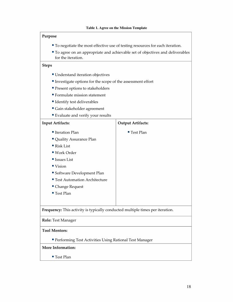
Each of these activities has a template that defines its structure, and can be

composed by: purpose, steps, input artefacts, output artefacts, frequency, role, tool

mentors, and additional information. An example is shown in Table 1 [11],

describing the activity Agree on the Mission.

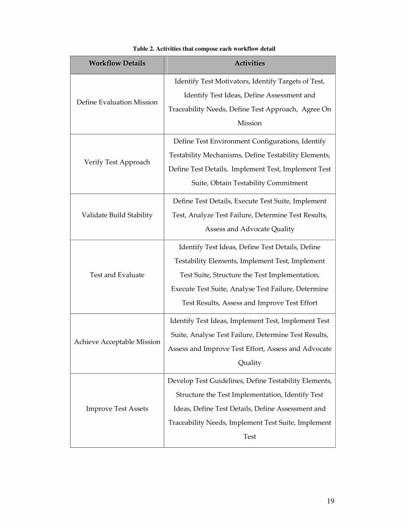
All of these activities can also be divided into groups that compose every

workflow detail of Figure 2. Table 2 shows the association between the activity

groups and the workflow details. Note that the same activity can be associated to

more than one workflow detail.

18

Table 1. Agree on the Mission Template

Purpose

� To negotiate the most effective use of testing resources for each iteration.

� To agree on an appropriate and achievable set of objectives and deliverables

for the iteration.

Steps

� Understand iteration objectives

� Investigate options for the scope of the assessment effort

� Present options to stakeholders

� Formulate mission statement

� Identify test deliverables

� Gain stakeholder agreement

� Evaluate and verify your results

Input Artifacts:

� Iteration Plan

� Quality Assurance Plan

� Risk List

� Work Order

� Issues List

� Vision

� Software Development Plan

� Test Automation Architecture

� Change Request

� Test Plan

Output Artifacts:

� Test Plan

Frequency: This activity is typically conducted multiple times per iteration.

Role: Test Manager

Tool Mentors:

� Performing Test Activities Using Rational Test Manager

More Information:

� Test Plan

19

Table 2. Activities that compose each workflow detail

Workflow Details Activities

Define Evaluation Mission

Identify Test Motivators, Identify Targets of Test,

Identify Test Ideas, Define Assessment and

Traceability Needs, Define Test Approach, Agree On

Mission

Verify Test Approach

Define Test Environment Configurations, Identify

Testability Mechanisms, Define Testability Elements,

Define Test Details, Implement Test, Implement Test

Suite, Obtain Testability Commitment

Validate Build Stability

Define Test Details, Execute Test Suite, Implement

Test, Analyze Test Failure, Determine Test Results,

Assess and Advocate Quality

Test and Evaluate

Identify Test Ideas, Define Test Details, Define

Testability Elements, Implement Test, Implement

Test Suite, Structure the Test Implementation,

Execute Test Suite, Analyse Test Failure, Determine

Test Results, Assess and Improve Test Effort

Achieve Acceptable Mission

Identify Test Ideas, Implement Test, Implement Test

Suite, Analyse Test Failure, Determine Test Results,

Assess and Improve Test Effort, Assess and Advocate

Quality

Improve Test Assets

Develop Test Guidelines, Define Testability Elements,

Structure the Test Implementation, Identify Test

Ideas, Define Test Details, Define Assessment and

Traceability Needs, Implement Test Suite, Implement

Test

20

2.2 Escaped Defects

Escaped defects can be defined as software defects that should be found by a test

team in a specific step of the process, and for some reason they have escaped. The

escaped defects analysis is the process of investigating these escapes, in order to

discover why they have escaped, prevent future escapes and then, making

preventive plans to avoid these future similar escapes [3]. This is important to

improve software quality, get better customer appreciation and also to reduce costs,

since whenever critical faults are exposed to the customers, there are great costs to

make software correction and maintenance.

The escape analysis process requires a lot of effort to get the best return. So, if

the development and test teams could both be involved, the process would produce

better results. According to [3], the objectives of escape analysis are to:

• Separate escapes into useful categories for further, more in-depth

analysis.

• Run statistics on the categorized data.

• Identify and implement overall process changes needed based on the

statistics.

• Identify and implement low-level (department-level) changes needed

based on in-depth analysis of specific escapes.

• Use metrics to demonstrate effectiveness of process changes.

There is also another preventive direction that can be followed with the

intention of reducing the escaped defects. This perspective considers the test cases

investigation, examining all existent test cases in a test suite and analysing, based on

defined criteria, which of them are more likely to allow as few escaped defects as

possible, in the context of a particular test suite execution.

Getting into this perspective, there are some possible ways to pursue: for

example, add more test cases to the group executed in the previous build, but this is

not the focus of this work; and select the most appropriate test cases from a suite (to

be explained in next section).

21

2.3 Regression Test Selection

Regression testing is the activity of testing a new version of a system in order to

validate this version, detecting whether bugs have been introduced due to the

changes made in the software, and thus, guaranteeing the correctness of the

modifications. Since the re-execution of all test cases in a suite is very expensive,

researchers have proposed techniques for reducing this expense, like regression test

selection [2], [6], [7] [14] [15], [16] and test suite minimization [17], [18] [19], [20], [21]

techniques.

Often there is a confusion between these two techniques, and in fact, they are

related but distinct. So, it is important to understand their differences. The test suite

minimization technique considers only the program and a test suite, and is

responsible to reduce the size of a test suite while still guaranteeing the same

coverage of the system functionalities. Regression test selection “reduces the cost of

regression testing by selecting an appropriate subset of the existing test suite, based

on information about the program, modified version, and test suite” [22].

Although these techniques are distinct they can be applied together, if the

objective is to attend both of their purposes, which is to select the minimal subset

from a test suite to validate a new build.

Both of these techniques can be unsafe. For instance, regression test selection,

which is the focus of this work, can have substantial cost, and worse, can disregard

test cases that could find bugs or consider tests that do not reveal faults at all,

reducing fault detection effectiveness. “This trade-off between the time required to

select and run test cases and the fault detection ability of the test cases that are run is

central to regression test selection.” [23]

Note that we can apply different approaches to this problem based on the

needs of the system. We can easily find researches that propose methods for

regression test selection, but almost all of them follow the white box strategy.

Looking for solving the Motorola company needs of reducing the escaped defects (in a

black box context) and making test case selection more efficient, this work is inspired

by the regression test selection idea, but considers a black box approach used in the

debugging field. We propose metrics that will be capable of selecting a subset of test

22

cases from a suite to validate a new version of the system. The solution proposed is

taken from research on debugging, in particular the fault prediction analysis. This is

explained in details in Chapter 4.

23

3 Debugging and Testing

Debugging is the process of locating and reducing the number of bugs in a

computer program code or the engineering of a hardware device, thus correcting its

wrong behaviour. Or, in few words, it is the process of “diagnosing the precise

nature of a known error and then correcting it” [29]. The most difficulty in debugging

is when the system is integrated, and various parts of the system are dependent on

each other, as changes made in one can interfere in another, introducing bugs to it.

Associating the activity of debugging with the RUP disciplines, it can be said

that debugging acts essentially in three disciplines, with different analysis to the

location of the failure for each one [30]. The first is the implementation discipline,

where developers introduce some errors that must be found quickly during

implementation or during the unit tests.

The next is during the test discipline, when the integration and system tests

are performed and some incorrect behaviour may happen. Here there is a careful

task to execute, before tracking the problem, which is to make sure that the problem

is with the system and not due to a bad test case specification or badly chosen data,

for example.

The last phase is the deployment, when the software product is tested to be

validated and finally available for the end users. Some specific undesirable

behaviours of the software can appear in this phase, such as inappropriate

performance or unsatisfactory recovery from a failure [30]. Thus, the portion of the

code that contains the problem needs to be found and fixed before it reaches the

customer.

So, as can be seen, the concept of debugging is, in some way, close to testing.

Software testing aims to validate the software. There are teams responsible to find

the system bugs and report to the development team, so they can solve these

problems. On the other hand, debugging is essentially performed by the developers,

where programmers often make use of debugging tools to help in program

inspection in order to find out what has caused the problem and how it might be

solved.

24

Zeller [34] proposes the basic steps in debugging, whose initial letters form the

word TRAFFIC:

• Track the problem. The first step in debugging is to track the problem,

i.e., to track and manage problem reports, that are archived in a problem

database – a document containing all problems found, and information

such as the situation that it has occurred (in order to understand how to

reproduce it), its severity level, and all known information that might

contribute to find the problem.

• Reproduce the failure. This step is responsible for creating instructions

to reproduce the problem. We have to specify a test case to be

performed in order to cause the program to fail as specified in the bug

report. There are two reasons for that [34]. The first is that you keep the

problem under control, since you can observe it whenever wanted. The

second is that after fixing the bug, its correctness can be verified.

• Automate and simplify. The objective here is to simplify the test case

specified, firstly trying to automate it, if necessary. Then, it is important

to try to simplify the test case inputs to acquire a smallest test case.

• Find infection origins. This step is the process of trying to discover the

possible causes of the problem. The source code of the program is

needed to determine its origins, and therefore, requires a good

knowledge of the system. There is a great difficulty in this step, since

the location of the bug is not always the same as its symptom.

• Focus on likely origins. The motivation here is to keep focus on the

most likely origins of the problem. Some rules that help following the

problem cause are: focus on infections, focus on causes, focus on anomalies,

focus on code smells, and focus on dependences. For more information about

each of them, see [34].

• Isolate the infection chain. The challenge here is to isolate the origin of

the infection. Then, continue isolating origins transitively until you

25

have an infection chain from the incorrect program code to its incorrect

program behavior [34].

• Correct the defect. This step is where the debugging phase itself is left

and programming and testing is returned, in order to apply the fix to

correct the defect. The testing is really important, as there is the need to

make sure that the system is performing the correct behavior and has

not inserted new bugs.

After fixing the bug, an important task that might be done is to learn anything

you can from that bug. For example, in [33] there are some suggestions, where a first

attempt may be to see whether the same programming error occurs in other parts of

the system, and whether new faults might be introduced after fixing the bug. Then,

you can ask yourself if that error could be prevented. In this case, how you could

have done differently to prevent it. Finally, you can analyze whether the bug could

be detected sooner and how to improve the test cases.

In this direction, there are some researches on debugging that provide studies

about how to predict faults [24], [25], [26], [27]. The basic idea of this approach is to

find locations where to focus the testing effort. Based on the idea summarized by Ko

et al. [28], which considers cognitive breakdown as the causes for faults introduced by

programmers, Kim at al. [25] assume that faults do not occur individually, but rather

in bursts of other related faults. Thus, they suggest that bug occurrences have four

different kinds of locality:

Changed-component locality: If a component was changed recently, it has a

great probability of introducing faults soon. This happens because any code

modification is considered a risk to introduce new faults, as we explained previously.

New-component locality: If a component has been added recently, it has a

great probability of introducing faults soon. A component added has the same

principle as the changed component, since it is also a code modification.

Temporal locality: If a component introduced a fault recently, it has a great

probability of introducing faults soon. An explanation for this assumption is that

26

programmers make their changes without knowing the correct or complete

specification of the system, thus injecting multiple faults [25].

Spatial locality: If a component introduced a fault recently, other components

that are close to that have a great probability of introducing faults soon. The

explanation for that is the same as for the temporal locality, since changes introduced

due to incorrect system knowledge, can be propagated over the rest of the system.

There are a lot of ways to calculate closeness. For example, components that belong

to the same file or directory are considered close components, in the sense of physical

locality. On the other hand, using logical coupling [31], [32], “two components are

close to each other (logically coupled) when they are frequently changed together”

[25]. Logical coupling is the method used in one of the criteria defined for the

selective regression test described in Chapter 4.

Based on that observations about bug localities, Kim at al. [25] developed an

algorithm, experimented on seven open source projects, that is 73%-95% precise at

predicting future faults at the file level. At the function/method level it can cover

about 46%-72% of future faults. Observing these statistics, this accuracy seems to be

really good, especially if compared with other experiments published. Thus, the

concept of bugs localities suggested is well indicated in order to predict faults, and

consequently, trying to prevent them.

Taking a deep look at the fault prediction approaches was possible to create a

bridge between debugging and testing, where fault prevention solutions shall be an

important practice to be used in software testing, and thus, obtaining great results.

To the best of our knowledge, there is no previous work in the literature addressing

this use of debugging concepts to improve the test process. So, this work might

provide an original contribution to that.

27

4 Test Selection Strategy

Looking for attending the Motorola needs of reducing escaped defects, a

strategy for test case selection was developed based on researches about debugging,

since, as already explained, no work found in literature about regression test

selection supports the black box technique. Thus, based mostly on interviews with

two members of the Motorola Execution Team and on the idea of preventing bugs,

five criteria (metrics) for selective regression test were proposed with the intention of

increasing coverage and, consequently, reducing the escaped defects.

The idea is to produce the relevance calculation of all test cases, based on each

metric, which is explained in details below. We also present their formal

specification. It is important to understand that every metric is treated independently

of the others, where each of them takes into account its own criterion. Thus, the test

case selection is done by using all metrics together. The most important criterion

depends on the current needs of the execution team.

Each section below presents one of the five criteria.

4.1 Test Case History

This metric considers the history (the number and status of the past executions)

of all test cases existent in the test suite. Table 3 shows a generic template for this

metric, containing its inputs, the solution proposed to get a selective regression test

based on this criterion, and the outputs. We use the same template for the other four

criteria defined in this section.

Table 3. Generic structure of Test Case History metric

The inputs

• For each test case, there is a history of its past executions (passed, failed,

blocked, etc).

The solution

• For each test case from the suite, calculate:

=

=≥

=

considered be tosize minimum N and otherwise 50%,

size executionslist | where N | if ,100*bugs Nº

|Τ|Τ%|Τ|T

ΗΗ

Ηf

28

The outputs:

• Test cases relevance order, based on the calculation result of each test case.

The solution for this metric is to calculate the number of times in which the

given test case has been executed and found an error, relative to the number of times

it was performed. The purpose is to treat the test cases with higher relevance as good

test cases to find errors, since they have a history tending to that. We only consider

tests which have run more than N times, where N is given by the user. Tests that

have not been executed at least N times are assigned to 50% chances of been selected.

4.1.1 Example

Suppose the test case “3” has a history as shown bellow. For the Motorola

Regression Test Team, the possible statuses of the test cases when they are performed

are: failed, blocked, passed and indeterminate. I will represent the status failed as “x” and

passed as “ok”. We assume N=5.

x ok x blocked x ok x x

The calculation result for the Test 3 using equation above is:

This indicates that the Test 3 has a relevance of 62, 5% for the first criterion.

This is the percentage of failed status in the whole test case history. Remember that

every test case from the suite contains a history, and therefore, has their specific

relevance percentage like the exemplified Test 3. Thus, with the result of all test cases

calculation, it is possible to select the most essential test cases for this criterion.

%5,62 %100*8

533 == T.:T ff

Test 3

29

4.1.2 Formal Specification

The formal specification for all metrics will follow the Z notation [35].

Expressions such as �: ���, �: ��|� • means “the set of expressions e which satisfies

p, where � � ��� and � � ��”.

The given sets used for all metrics are:

[ T ] Set of Tests Cases

[ C ] Set of Components

For this particular, its formal specification is:

� �� ����� �, ���� �, ��� � ������ , ����� ��

� ���� 1: ! " � # �$ % & " ! " '$

( !): ! " � # �, �:& •

� ���� 1 !), �$ � *�: !|� � ��� !) + #-!) �$. / � • � 0 #-!) �$ 1 ����� ��.#-!) �$. 2 100%5

6 ��: !|� � ��� !) + # !) �$ 7 �$ • � 8 50%�

where the symbol ”1” represents the filter operator. If s is a sequence, then s 1 A is the

largest subsequence of s containing only those objects that are elements of A:

:�, �, �, �, , �, �, �, �; 1 ��, �� � :�, �, �, �; [35].

30

4.2 Changed and New Components

This metric follows the principle of Changed-component locality and New-

component locality presented in Chapter 3. Interviewing two members of the Motorola

Execution Teams, it was possible to notice that these approaches are also used

intuitively by them. Table 4 presents the generic structure for this metric.

Table 4. Generic structure of Changed and New Components metric

The inputs

• For each test case:

- C: the set of components visited by the test case.

- M: the set of changed and new components for the current build.

The solution

• For each test case from the suite, calculate:

The outputs:

• Test cases relevance order, based on the calculation result of each test case.

This solution considers the percentage of changed and new components for the

current build that a given test case covers. In this way, it is possible to know which

test cases are more relevant for this criterion, namely, the ones that present the higher

percentages.

4.2.1 Example

We show below the sets “C” and “M”. “C” is the set of components the test 3

visits. “M” is the set of modified and new components of the current build. Note that

the components “C1”, “C3” and “C4” are the intersection between “C” and “M”.

%100*||

||

M

MCTf ∩

=

31

The calculation result for the Test 3 using the equation presented is:

This shows that the test case “3” visits 42,86% of the changed and new

components for the current build. Again, this is an example for just one test case.

This calculation has to be done for all test cases from the suite. Finally, with the result

of all calculations, the more relevant test cases can be selected.

4.2.2 Formal specification

� ���� 2: ! = >$ % ?>$ " ! " '$ ( !>: ! @ >,�:?> •

� ���� 2 !>,�$ � A�: !|� � ��� !> + # � B 0 • � 8 # !>C���DE�$# � 2 100%F

Note: the symbol “C D” is denoting the relational image of t under TC. This is

the set of all elements in C to which some element of t is related [35].

%86,42 %100*7

333 ≈= T.:T ff

Test 3 Build

C M

C1

C2

C3

C4

1

C1

C4C3

C5C9

11 C10

111

C7

32

4.3 Recent Failures

Again, this metric was defined based on the interviews with the Motorola

Execution Team members, which naturally follow the idea of preventing future

faults by paying attention to the more recent failures that appeared at the system

under test. If you can remember, this approach has the same intention of the temporal

locality presented in Chapter 3, which considers any component with recent failures

as suspects to fail again.

Now, it is important to know the concept of a CR (Change Request): a

documentation that indirectly contains a report about a bug occurrence by requesting

a system modification to correct it. Table 5 shows the structure for this criterion.

Table 5. Generic structure of Recent Failures metric

The inputs

• The components that failed in the previous build.

• For each of these components, the percentage of CRs opened in the previous

build (already normalized).

• For each of these components, the set of associated test cases.

The solution

• For each test case from the suite:

- Calculate the sum of all percentages associated to that test case.

The outputs:

• Test cases relevance order, based on the calculation result of each test case.

This solution is very simple: it just adds the percentage associated to each test

case from the suite. Note that if some test case does not visit any recently failed

component it will receive 0% of relevance for this metric.

4.3.1 Example

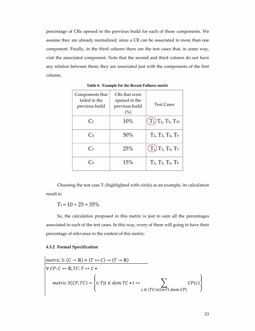
Suppose that, in the previous build, the system under test presented failures at

the components shown in the Table 6 (first column). The second column contains the

33

percentage of CRs opened in the previous build for each of those components. We

assume they are already normalized, since a CR can be associated to more than one

component. Finally, in the third column there are the test cases that, in some way,

visit the associated component. Note that the second and third column do not have

any relation between them; they are associated just with the components of the first

column.

Table 6. Example for the Recent Failures metric

Components that

failed in the

previous build

CRs that were

opened in the

previous build

(%)

Test Cases

C2 10% T1, T2, T9, T10

C4 50% T2, T3, T4, T6

C5 25% T1, T3, T4, T5

C9 15% T3, T5, T6, T8

Choosing the test case T1 (highlighted with circle) as an example, its calculation

result is:

T1 = 10 + 25 = 35%

So, the calculation proposed in this metric is just to sum all the percentages

associated to each of the test cases. In this way, every of them will going to have their

percentage of relevance to the context of this metric.

4.3.2 Formal Specification

� ���� 3: > " '$ % ! @ >$ " ! " '$ ( >H: > @ ', !>: ! @ > •

� ���� 3 >H, !>$ � I�: !|� � ��� !> • � 8 J >H �$� � -!>C���DE ��� >H.K

34

4.4 Escaped Defects

This is a more specific attempt of reducing the escaped defects. The idea is to

try to prevent that the same components which presented escaped defects, present it

again. Based on the strategy defined for the previous metric, this one is very similar

to that, and there are two differences due to its context: here we consider components

that presented escaped defects at a specific period of time, while the other criteria

considered just the previous build. The test cases to be considered are just the ones

that were not performed (the test cases that were performed are not important for

this metric and can be considered as they received 0% of relevance).

The justification for these differences is, firstly, that the Motorola Execution

Team makes a survey of escaped defects and creates a graph containing the

percentage of CRs that escaped from the BTC per components in a certain period of

time. This graph provides the inputs for this metric.

The second difference is that we consider only test cases that were not

performed due to the fact that we are not interested in test cases that were executed

in the specific period of time but did not found the defects that escaped. All that

matters here is to try to avoid the escapes. The idea is to include some test cases from

the suite that were not executed and which can possibly find some of those defects.

Table 7 shows the structure for this metric.

Table 7. Generic structure of Escaped Defects metric

The inputs

• The components that presented escaped defects at a specific period of time.

• For each of these components, the percentage of CRs (also already

normalized) that escaped BTC (Brazil Test Center).

• For each of these components, the set of associated test cases, that was not

performed at that specific time.

The solution

• For each test case that was not performed at the specific time:

35

- Calculate the sum of all percentages associated to that test case.

The outputs:

• Test cases relevance order, based on the calculation result of each test case.

As you can see, the solution for this metric is the same as the previous one. The

only difference is that the test cases to be considered are not the whole test suite, but

just the ones that were not performed in the specified time. The remaining test cases

are not important for this metric, thus, can be considered as test cases with 0% of

relevance.

4.4.1 Example

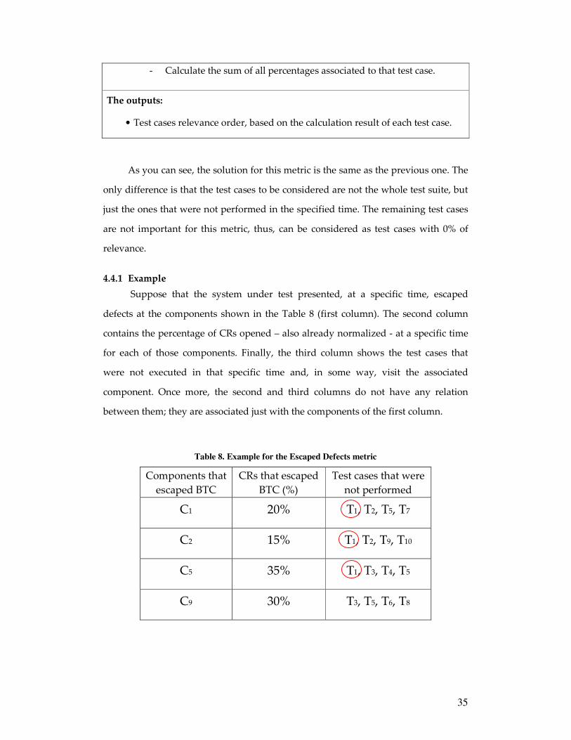
Suppose that the system under test presented, at a specific time, escaped

defects at the components shown in the Table 8 (first column). The second column

contains the percentage of CRs opened – also already normalized - at a specific time

for each of those components. Finally, the third column shows the test cases that

were not executed in that specific time and, in some way, visit the associated

component. Once more, the second and third columns do not have any relation

between them; they are associated just with the components of the first column.

Table 8. Example for the Escaped Defects metric

Components that

escaped BTC

CRs that escaped

BTC (%)

Test cases that were

not performed

C1 20% T1, T2, T5, T7

C2 15% T1, T2, T9, T10

C5 35% T1, T3, T4, T5

C9 30% T3, T5, T6, T8

36

Again, choosing the test case T1 (highlighted with circle) as an example, the

calculation result for it is:

T1 = 20 + 15 + 35 = 70%

So, the calculation proposed in the solution for this metric is just to sum all the

percentages associated to each of the test cases. Just like the Recent Failures metric

does.

4.4.2 Formal Specification

As the calculation for this metric is the same as the previous one, its formal

specification is the same too. The only difference is that this one considers only the

test cases not performed.

Consider, for this metric, the given set:

[ T’ ] Set of Tests Cases not performed in some specific time

� ���� 4: > " '$ % !M @ >$ " !M " '$ ( >H: > @ ', !>: !M @ > •

� ���� 4 >H, !>$ � N�: !M|� � ��� !> • � 8 ∑ >H �$� � !>C���DE ��� >H$ P

37

4.5 Spatial Locality

This metric is based on the Spatial locality suggested by Kim et al. [25] (see

Chapter 3). Recall that components very close to components that failed recently are

considered suspects to fail too. So, once the set of components that failed recently is

known, the task here is to analyze the remaining components in order to discover

which of them are the suspects of introducing errors.

In order to calculate the distance between two components, the notion of

logical coupling is used (also explained in Chapter 3). The distance formula we

present here is a little bit different from the one presented by Kim et al. [25] (we do

not use infinite values as opposed to Kim et al. See more details below). By using the

equation, we calculate the distance between every component that failed recently

and every remaining component.

After calculating those distances, the purpose is to analyze the components

closer to the recently failed components. The relevant test cases are those associated

to the suspect components. The structure of this metric is shown in Table 9, which

explains the solution in detail.

Table 9. Generic structure of Spatial Locality metric

The inputs

• V1, V2 … Vn: History of versions, where each version is the set of new and

changed components of that version.

• C’: the set of components that failed in the previous build.

• C’’: the remaining components.

• Every set of test cases associated to each C’’.

The solution

• Calculate the distance between every C’ and C’’ using equation:

=

>

=

0 if , 2

0 if ,),(

1

),(

21

21

2121

) ,Ccount(C

) ,Ccount(CCCcountCCdistance

getherchanged to have been and C times C number of) ,Ct(Cwhere coun 2121 =

38

As said before, the solution consists, firstly, of calculating the distances

between every component c’ � C’ that failed in the previous build and every

remaining component c’’ � C’’. The distances are calculated using the equation

shown in the solution of Table 9, which considers the number of times two

components have been changed together. The closer they are the smaller the distance

between them. Due to this fact, the distance is the inverse of count.

Kim at al. [25] considers that the distance between two components that have

count equals to zero is infinite. We are assigning 2 instead of infinite, because as we

need to calculate the average distance, it would be impracticable to use infinite. Since

the greater result possible is 1 (whenever count is 1), using 2 for very distant

components seems to be a good compromise.

After calculating all distances, the next step is to investigate the components of

C’’ that are very close to the components of C’ by calculating their average distance.

Remember that we are considering just the distances of every C’’ and not the

distances of the components in C’, because this metric considers only the components

that are close to the components that failed recently, treating them as suspects too.

Note that the components of C’ are already covered in the Recent Failures metric

(section 0).

Now, with the average distances in hands, the next step is similar to the two

previous metrics. We have to normalize these averages to 100%, and then, we build a

table like Table 6 and Table 8. The procedure to generate this final step is the same

from the previous metric. The example shall clarify this metric.

• Calculate the average distance related to every C’’.

• Calculate the percentage related to every C’’ by assigning the value “2 -

average” and then, normalizing to 100%.

• For each test case from the suite:

- Calculate the sum of the percentages associated to that test case.

The outputs:

• Test cases relevance order, based on the calculation result of each test case.

39

4.5.1 Example

Suppose that the system under test has a version history (V1, V2 … V5) like this

one shown below.

Then, suppose that C’ and C’’ are:

Now, we calculate the distance between every c’ � C’ and c’’ � C’’ by using the

equation presented in the field solution (Table 9). As an example, let’s calculate the

distance between C1 and C5. Firstly, we have to count the number of times in which

these components have been changed together (see the count in the equation shown

in Table 9). Looking to the versions (V1 … V5) we can see that they appear together

four times, that is:

So, the distance is:

Continuing the calculation of the distances between every C’ and C’’, the Table

10 is produced. The distance between C1 and C5 is highlighted with circle.

C1

C2 C4

C3

C’

C6

C7 C5

C8

C9

C’’

4=),Ccount(C 51

25,04

1),( 51 ==CCdistance

V1

C1

C2 C5

C3

V2

C1

C5

C9 C7

C1

C3 C4C5

C7

V3

C1

C5

C6C7

C8C9

V4

C2

C5

C7

V5

40

Table 10. Distances

Having all distances calculated for every c’’ � C’’, it is time to calculate their

respective averages. For example, the average distance for C5 will be:

After calculating the averages for every c’’ � C’’, we can build the Table 11

below.

Table 11. Averages of every c’’ � C’’ and the associated test cases

C

5 C

6 C

7 C

8 C

9

C1 0,25 1 0,33 1 0,5

C2 0,5 2 1 2 2

C3 0,5 2 1 2 2

C4 1 2 1 2 2

Components

(C’’) Averages Test cases

C5 0,56 T1,

T2,

T9,

T10

C6 1,75 T2,

T3,

T7,

T6

C7 0,83 T1,

T3,

T4,

T5

C8 1,75 T3,

T5,

T6,

T8

C9 1,62 T2,

T5

56,04

15,05,025,0≅

+++=)average(C5

C’ C’’

41

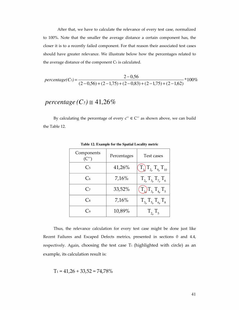
After that, we have to calculate the relevance of every test case, normalized

to 100%. Note that the smaller the average distance a certain component has, the

closer it is to a recently failed component. For that reason their associated test cases

should have greater relevance. We illustrate below how the percentages related to

the average distance of the component C5 is calculated.

By calculating the percentage of every c’’ � C’’ as shown above, we can build

the Table 12.

Table 12. Example for the Spatial Locality metric

Thus, the relevance calculation for every test case might be done just like

Recent Failures and Escaped Defects metrics, presented in sections 0 and 4.4,

respectively. Again, choosing the test case T1 (highlighted with circle) as an

example, its calculation result is:

T1 = 41,26 + 33,52 = 74,78%

Components

(C’’) Percentages Test cases

C5 41,26% T1,

T2, T9,

T10

C6 7,16% T2,

T3,

T7,

T6

C7 33,52% T1,

T3,

T4,

T5

C8 7,16% T3,

T5,

T6,

T8

C9 10,89% T2,

T5

%100*)62,12()75,12()83,02()75,12()56,02(

56,02

−+−+−+−+−

−=)(Cpercentage 5

%26,41≅)(Cpercentage 5

42

4.5.2 Formal Specification

) �� ? ?>$ : Set of all changed components histories

��Q��: > % > % ) " ' (�₁, �₂ T >, U T ) •

��Q�� �₁, �₂, U$ � #�V:?>|��₁, �₂� W V + V � U�

������� : > % > % ) " ' (�₁, �₂ T >, U T ) • ������� �₁, �₂, U$ � I 1��Q��-�₁,�₂,U. , � � X U + U B ø + ��Q�� �₁, �₂, U$ Z 0 2, � � X U + U B ø + ��Q�� �₁, �₂, U$ � 0K

������� �: ?>$ % ?>$ % ) " - > % >$ " '. ( �Q[�, ��U ��: ?>, U:) • ������� � �Q[�, ��U ��, U$ �

��Q[, ��U �: >; U:)|U B ø + � � X U + �Q[� ] ��U �� � ø$ + �Q[� ^ ��U �� � >$

+ �Q[ � �Q[� + ��U � � ��U �� • �Q[, ��U �$ " ������� �Q[, ��U �, U$�

�V ��[ : -> % > % > " '$. " ' ( ��U �: >, ��: > % >$ " ' •

�V ��[ ��U �, ��$ � ∑ ��-�,��U �.���Q[�# �Q[� , _U � �Q[� � ���� ��� ��$� B 0

43

�V ��[ �: > % > " '$ " > " '$ ( ��: > % > " '$ •

�V ��[ � ��$ � ��Q[, ��U �: >| �Q[, ��U �$ � ��� �� • ��U � "

�V ��[ ��U �, ��$�

�������` : > " '$ " > " '$ ( ��: > " '$ •

�������` ��$ �abcbd�: >, �:'| �, �$ � �� • > " -2e�.

∑ f2e�Mg h�M,�Mi � ��

2 100%jbkbl

� ���� 5: ?> % ?> % ) % ! @ >$ " ! " '$ ( �Q[�:?>, ��U ��: ?>, U: ), !>: ! @ >$ • � ���� 5 �Q[�, ��U ��, U, !>$ �� ���� 4 m�������` m�V ��[ �-������� � �Q[�, ��U ��, U$.n , !>n

44

5 Experiments

In this chapter we will suppose a small system and use the metrics described in

the previous section in order to get the results to the regression test selection. As

already explained, all metrics provide a test case relevance order where one can

choose the ones with higher percentages as good test cases to find errors in the

system. The metrics were implemented in Python1 and the results are presented

sorted in a decreasing relevance order.

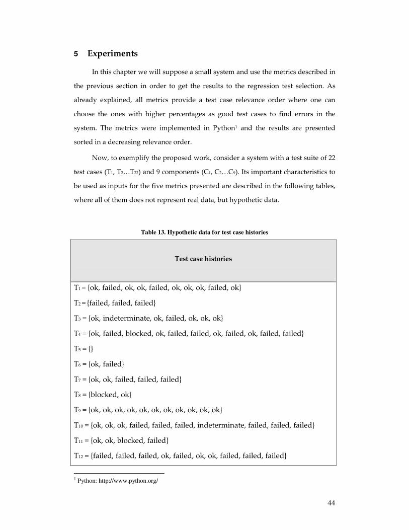
Now, to exemplify the proposed work, consider a system with a test suite of 22

test cases (T1, T2…T22) and 9 components (C1, C2…C9). Its important characteristics to

be used as inputs for the five metrics presented are described in the following tables,

where all of them does not represent real data, but hypothetic data.

Table 13. Hypothetic data for test case histories

Test case histories

T1 = {ok, failed, ok, ok, failed, ok, ok, ok, failed, ok}

T2 = {failed, failed, failed}

T3 = {ok, indeterminate, ok, failed, ok, ok, ok}

T4 = {ok, failed, blocked, ok, failed, failed, ok, failed, ok, failed, failed}

T5 = {}

T6 = {ok, failed}

T7 = {ok, ok, failed, failed, failed}

T8 = {blocked, ok}

T9 = {ok, ok, ok, ok, ok, ok, ok, ok, ok, ok, ok}

T10 = {ok, ok, ok, failed, failed, failed, indeterminate, failed, failed, failed}

T11 = {ok, ok, blocked, failed}

T12 = {failed, failed, failed, ok, failed, ok, ok, failed, failed, failed}

1 Python: http://www.python.org/

45

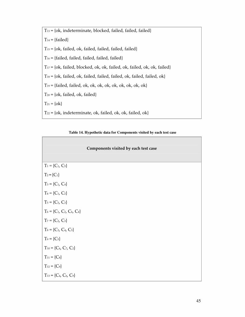
T13 = {ok, indeterminate, blocked, failed, failed, failed}

T14 = {failed}

T15 = {ok, failed, ok, failed, failed, failed, failed}

T16 = {failed, failed, failed, failed, failed}

T17 = {ok, failed, blocked, ok, ok, failed, ok, failed, ok, ok, failed}

T18 = {ok, failed, ok, failed, failed, failed, ok, failed, failed, ok}

T19 = {failed, failed, ok, ok, ok, ok, ok, ok, ok, ok, ok}

T20 = {ok, failed, ok, failed}

T21 = {ok}

T22 = {ok, indeterminate, ok, failed, ok, ok, failed, ok}

Table 14. Hypothetic data for Components visited by each test case

Components visited by each test case

T1 = {C1, C5}

T2 = {C1}

T3 = {C1, C4}

T4 = {C1, C2}

T5 = {C5, C3}

T6 = {C1, C2, C6, C4}

T7 = {C2, C3}

T8 = {C3, C4, C5}

T9 = {C5}

T10 = {C6, C7, C2}

T11 = {C8}

T12 = {C9}

T13 = {C4, C6, C9}

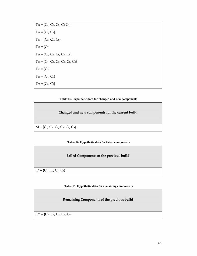
46

T14 = {C4, C6, C7, C8, C9}

T15 = {C3, C9}

T16 = {C2, C6, C8}

T17 = {C7}

T18 = {C2, C4, C6, C8, C9}

T19 = {C1, C2, C3, C5, C7, C8}

T20 = {C3}

T21 = {C4, C6}

T22 = {C8, C9}

Table 15. Hypothetic data for changed and new components

Changed and new components for the current build

M = {C1, C2, C4, C6, C8, C9}

Table 16. Hypothetic data for failed components

Failed Components of the previous build

C’ = {C1, C2, C5, C8}

Table 17. Hypothetic data for remaining components

Remaining Components of the previous build

C’’ = {C3, C4, C6, C7, C9}

47

Table 18. Hypothetic data for the percentage of CRs opened for the failed components

Percentages of CRs opened for each failed component of the previous build

C1 = 13%

C2 = 48%

C5 = 31%

C8 = 8%

Table 19. Hypothetic data for the components that presented escaped defect

Components that presented escaped defects in a period of 3 months

E = {C4, C5, C6}

Table 20. Hypothetic data for the percentages of CRs opened for escaped defects components

Percentages of CRs opened for each component that presented escaped defects in

a period of 3 months

C4 = 26%

C5 = 43%

C6 = 31%

Table 21. Hypothetic data for the test cases not performed

Test cases that were not performed in the period of 3 months

Tn = {T5, T9, T8, T13, T20, T21}

48

Table 22. Hypothetic data for the history of versions

The versions of changed components in all previous versions

V1 = {C1, C3, C4, C5, C8, C9}

V2 = {C1, C3, C7}

V3 = {C2, C3, C5, C6, C8}

V4 = {C9, C4, C5}

V5 = {C2, C5, C7, C9}

V6 = {C1, C4, C3, C6, C9}

V7 = {C2, C4, C8, C9}

5.1 Results

Considering all the hypothetic data presented in the tables above, the results of

each metric are shown in the Table 23. Each metric needs a particular subset of those

data as inputs to provide their results, such:

• The first metric (Test Case History - section 4.1) considers the test case

histories presented in Table 13 and also considers that N = 3;

• The second metric (Changed and New Components - section 4.2)

considers the changed and new components for the current build,

presented in Table 15 and the components visited by each test case

(Table 14);

• The third metric (Recent Failures - section 4.3) considers the failed

components of the previous build (Table 16), the percentage of CRs

opened for each of those components (Table 18) and again, the

components visited by each test case (Table 14);

49

• The fourth metric (Escaped Defects - section 4.4) considers the

components that presented BTC escaped defects in the specified period

of time (3 months, in this case) shown in Table 19, the percentage of CRs

opened for each of those components (Table 20) and of course, the

components visited by each test case that were not performed at this

time (Table 14 and Table 21);

• Finally, the last metric (Spatial Locality – section 4.5) considers the

versions of changed components in all previous versions (Table 22), the

failed components of the previous build (Table 16), the remaining

components (Table 17) and then, the components visited by each test

case (Table 14).

Table 23. The results of all metrics

Metric 1 Metric 2 Metric 3 Metric 4 Metric 5

T2 = 100%

T16 = 100%

T15 = 71,43%

T12 = 70%

T7 = 60%

T18 = 60%

T10 = 60%

T4 = 54,55%

T8 = 50%

T6 = 50%

T5 = 50%

T21 = 50%

T20 = 50%

T14 = 50%

T18 = 83,33%

T6 = 66,67%

T14 = 66,67%

T19 = 50%

T16 = 50%

T13 = 50%

T4 = 33,33%

T3 = 33,33%

T22 = 33,33%

T21 = 33,33%

T10 = 33,33%

T8 = 16,67%

T7 = 16,67%

T2 = 16,67%

T19 = 100%

T6 = 61%

T4 = 61%

T18 = 56%

T16 = 56%

T7 = 48%

T10 = 48%

T1 = 44%

T9 = 31%

T8 = 31%

T5 = 31%

T3 = 13%

T2 = 13%

T22 = 8%

T8 = 69%

T21 = 57%

T13 = 57%

T9 = 43%

T5 = 43%

T20 = 0%

T14 = 76,71%

T18 = 64,38%

T13 = 64,38%

T15 = 48,63%

T8 = 45,89%

T6 = 39,04%

T21 = 39,04%

T19 = 35,62%

T10 = 28,77%

T22 = 25,34%

T12 = 25,34%

T7 = 23,29%

T5 = 23,29%

T20 = 23,29%

50

T13 = 50%

T17 = 36,36%

T1 = 30%

T22 = 25%

T11 = 25%

T19 = 18,18%

T3 = 14,29%

T9 = 0%

T15 = 16,67%

T12 = 16,67%

T11 = 16,67%

T1 = 16,67%

T9 = 0%

T5 = 0%

T20 = 0%

T17 = 0%

T14 = 8%

T11 = 8%

T21 = 0%

T20 = 0%

T17 = 0%

T15 = 0%

T13 = 0%

T12 = 0%

T3 = 22,6%

T16 = 16,44%

T17 = 12,33%

T9 = 0%

T4 = 0%

T2 = 0%

T11 = 0%

T1 = 0%

It is worth emphasizing that with these results of all metrics, the manager

of the execution test team can analyse carefully each of them, and based on

the needs and priorities of the current build, can select the best test cases to be

re-run.

51

6 Conclusion

This work has proposed a method to regression test case selection in order to

reduce escaped defects. Tending to that, five metrics were defined to be used on the

test case selection, separately. They were based mostly on interviews with the

Motorola Execution Team and researches on debugging, more specifically on faults

prediction. In this way, preventing bugs shall be an interesting idea to reduce defects

to escape.

The major contribution of this work is the use of debugging techniques to

increase the reliability of software testing, in this case, regression test selection. The

five metrics were also implemented in the Python language in order to exemplify

these metrics and take a deep look on how they work. Analysing carefully each of

them, and prioritizing the most relevant ones for the particular situation,

appropriated test case selection shall me possible.

6.1 Related Work

Once we have made use of predicting fault techniques to regression test case

selection, there are two kinds of related work.

In [36], for example, the authors have proposed three regression test selection

methods with the purpose of reducing the number of selected test cases. In addition,

they have also suggested two regression test coverage metrics to address the

coverage identification problem, based on McCabe [37]. To study the veracity of their

proposed methods they have empirically compared the three methods with other

three reduction and precision-oriented methods.

In [25], Kim at. Al. developed an algorithm based on the concept of bug

occurrence locality, like was already explained in section 3. Following the idea of [38]

they used the notion of a cache from operating systems to predict faults by caching

locations with great probabilities of having faults. They have experimented their

algorithm on seven open source projects and the cache selected 10% of the source

code files where these files account for 73%-95% of faults.

52

6.2 Future Works

The future works that can be highlighted for this work are:

• To do more experiments in order to validate the metrics defined.

Mostly, it is important to do a case study within Motorola, using real

examples to experiment.

• Introduce the new metrics defined to the Motorola Execution Team,

thus they can use them and report any problem or suggestion of

improvement if necessary.

• Mechanise everything, which seems to be a big challenge, once the job

of join all the inputs to be used for the metrics is really hard. This fact is

due to these inputs being very disperse in the Motorola documents.

53

References

[1] P. Kruchten, “The Rational Unified Process”, Addison-Wesley, 1998.

[2] D. Binkley, “Semantics guided regression test cost reduction” IEEE

Transactions on Software Engineering, 23(8): 498-516, August 1997.

[3] M. A. Vandermark, "Defect Escape Analysis: Test Process Improvement"

STAREAST 2003: Proceedings of the Software Testing Analysis and Review

Conference, May 2003.

[4] R. Patton, “Software Testing” (2nd Edition), 2005.

[5] J. Pan, “Software Testing”, Carnegie Mellon University, 1999.

[6] G. Rothermel, M. J. Harrold, "Analyzing Regression Test Selection

Techniques" IEEE Transactions on Software Engineering, vol. 22, no. 8, pp.

529-551, August 1996.

[7] H. Agrawal, J. Horgan, E. Krauser, S. London, "Incremental Regression

Testing" In Proceedings of the Conference on Software Maintenance, pages 348-

357, September 1993.

[8] W. Hetzel, “The Complete Guide to Software Testing”, 2nd ed. Publication

info: Wellesley, Mass.: QED Information Sciences, 1988.

[9] Qualiti, Programa de Qualificação Tecnológica - “Introdução a Testes de

Software” (In Portuguese).

[10] P. Szymkowiak, P. Kruchten, Testing: “The RUP Philosophy”, Copyright

Rational Software, 2003.

[11] “Rational Unified Process: Overview”, Copyright Rational Software

Corporation, 1987 – 2001.

[12] “Cycoda: The Test discipline”, Copyright 2004 - 2007 Cycoda Limited,

available at: http://www.cycoda.com/swDev/RUP/Test/test.html.

[13] IBM Software Group, P17 System Testing, “Module 6: Testing Iteratively”,

September 2007.

54

[14] Y. F. Chen, D. S. Rosenblum, K. P. Vo, “TestTube: A system for selective

regression testing” In Proceedings of the 16th International Conference on

Software Engineering, pages 211-222, May 1994.

[15] H. K. N. Leung, L. J. White, “A study of integration testing and software

regression at the integration level.” In Proceedings of the Conference on

Software Maintenance, pages 290-300, November 1990.

[16] G. Rothermel, M. J. Harrold, “A safe, efficient regression test selection

technique.” ACM Transactions on Software Engineering and Methodology,

6(2):173-210, April 1997.

[17] J. von Ronne, "Test Suite Minimization: an Empirical Investigation" PhD

thesis. Oregon State University, 1999.

[18] T. Y. Chen, M. F. Lau, “Dividing strategies for the optimization of a test

suite.” Information Processing Letters, 60(3):135-141, March 1996.

[19] M. J. Harrold, R. Gupta, M. L. So_a, “A methodology for controlling the size

of a test suite.” ACM Transactions on Software Engineering and Methodology,

2(3):270-285, July 1993.

[20] G. Rothermel, M. J. Harrold, J. Ostrin, C. Hong, “An empirical study of the

effects of minimization on the fault detection capabilities of test suites.” In

Proceedings of the International Conference on Software Maintenance, pages 34-

43, November 1998.

[21] W. E. Wong, J. R. Horgan, S. London, A. P. Mathur, “Effect of test set

minimization on fault detection effectiveness.” Software - Practice and

Experience, 28(4):347-369, April 1998.

[22] G. Rothermel, R. H. Untch, C. Chu, M. J. Harrold, “Prioritizing test cases for

regression test.” IEEE Transactions on Software Engineering, vol. 27, no. 10,

pp. 929-948, October 2001.

[23] T. L. Graves, M. J. Harrold, J. Kim, A. Porter, G. Rothermel, “An empirical

study of regression test selection techniques” ACM Transactions on Software

Engineering and Methodology, vol. 10, no. 2, pp. 184-208, April 2001.

55

[24] A. Schröter, T. Zimmermann, R. Premraj, A. Zeller, “Where Do Bugs Come

From? A Challenge for Empirical Software Engineering”, ACM SIGSOFT

Software Engineering Notes, vol. 31, pp. 1-2, November 2006.

[25] S. Kim, T. Zimmermann, E. J. Whitehead, Jr., A. Zeller, “Predicting Faults

from Cached History”, Proceedings of the 29th International Conference on

Software Engineering (ICSE 2007), pp. 489–498, May 2007.

[26] T. L. Graves, A. F. Karr, J. S. Marron, H. Siy, "Predicting Fault Incidence

Using Software Change History," IEEE Transactions on Software Engineering,

vol. 26, pp. 653-661, 2000.

[27] A. E. Hassan and R. C. Holt, "The Top Ten List: Dynamic Fault Prediction,"

Proceedings of International Conference on Software Maintenance (ICSM 2005),

Budapest, Hungary, 2005, pp. 263-272.

[28] A. J. Ko, B. A. Myers, "A Framework and Methodology for Studying the

Causes of Software Errors in Programming Systems," Journal of Visual

Languages and Computing, vol. 16, pp. 41-84, 2005.

[29] G. J. Myers, “Software Reliability: Principles and Practices”, John Wiley &

Sons, Inc., New York, 1976.

[30] B. Hailpern, P. Santhanam, “Software debugging, testing, and verification”,

IBM Systems Journal, vol. 41, no. 1, pp. 4-12, 2002.

[31] J. Bevan and E. J. Whitehead, Jr., "Identification of Software Instabilities",

Proceedings of 2003 Working Conference on Reverse Engineering (WCRE 2003),

Victoria, Canada, 2003.

[32] H. Gall, M. Jazayeri, and J. Krajewski, "CVS Release History Data for

Detecting Logical Couplings," Proceedings of Sixth International Workshop on

Principles of Software Evolution (IWPSE' 03), Helsinki, Finland, pp. 13-23,

2003.

[33] I. L. Taylor, “Debugging”, Copyright 2003 by Ian Lance Taylor, available at:

http://www.airs.com/ian/essays/debug/debug.html#AEN110, last access in

May/2008.

56

[34] A. Zeller, “Why program fail – A Guide to Systematic Debugging”, Morgan

Kaufmann Publishers Inc. San Francisco, CA, USA, 2005.

[35] J. Woodcock, J. Davies, “Using Z – Specification, Refinement, and proof”.

[36] R. Bahsoon, N. Mansour, "Methods and Metrics for Selective Regression

Testing,", ACS/IEEE International Conference on Computer Systems and

Applications (AICCSA'01), pp. 463-465, 2001.

[37] T. McCabe, “A complexity measure”, IEE Trans. On Software Engineering,

pp. 308-319, December 1976.

[38] A. E. Hassan, R. C. Holt, “The top ten list: dynamic fault prediction”,

Proceedings of International Conference on Software Maintenance (ICMS 2005),

Budapest, Hungary, pp. 263-272, 2005.

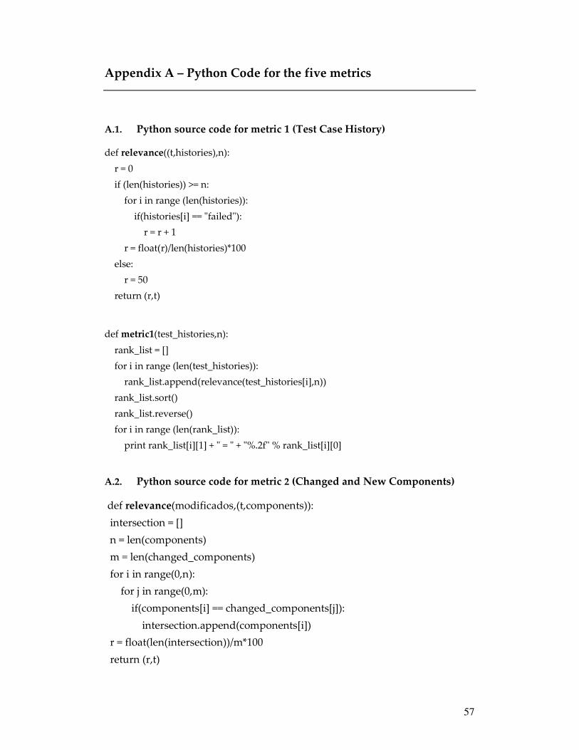
57

Appendix A – Python Code for the five metrics

A.1. Python source code for metric 1 (Test Case History)

def relevance((t,histories),n):

r = 0

if (len(histories)) >= n:

for i in range (len(histories)):

if(histories[i] == "failed"):

r = r + 1

r = float(r)/len(histories)*100

else:

r = 50

return (r,t)

def metric1(test_histories,n):

rank_list = []

for i in range (len(test_histories)):

rank_list.append(relevance(test_histories[i],n))

rank_list.sort()

rank_list.reverse()

for i in range (len(rank_list)):

print rank_list[i][1] + " = " + "%.2f" % rank_list[i][0]

A.2. Python source code for metric 2 (Changed and New Components)

def relevance(modificados,(t,components)):

intersection = []

n = len(components)

m = len(changed_components)

for i in range(0,n):

for j in range(0,m):

if(components[i] == changed_components[j]):

intersection.append(components[i])

r = float(len(intersection))/m*100

return (r,t)

58

def metric2(test_components,changed_components):

rank_list = []

for i in range (len(test_components)):

rank_list.append(relevance(changed_components, test_components[i]))

rank_list.sort()

rank_list.reverse()

for i in range (len(rank_list)):

print rank_list[i][1] + " = " + "%.2f" % rank_list[i][0]

A.3. Python source code for metrics 3 and 4 (Recent Failures and Escaped

Defects)

def relevance(crs, (t,components)):

r = 0

for i in range (len(components)):

for j in range (len(crs)):

if (components[i] in crs[j][0]):

r = r + crs[j][1]

return (r,t)

def metric3_4(test_components,crs):

rank_list = []

for i in range (len(test_components)):

rank_list.append(relevance(crs, test_components[i]))

rank_list.sort()

rank_list.reverse()

for i in range (len(rank_list)):

print rank_list[i][1] + " = " + "%.2f" % rank_list[i][0]

A.4. Python source code for metric 5 (Spatial Locality)

def distance(comp1, comp2,versions):

count = 0

dist = 0

for i in range (len(versions)):

if (comp1 in versions[i][1] and comp2 in versions[i][1]):

59

count = count + 1

if(count > 0):

dist = float(1)/count

else:

dist = 2

return dist

def distances(failed_comp,remaining_comp,versions):

distances_list = []

for i in range (len(failed_comp)):

for j in range (len(remaining_comp)):

distances_list.append(((failed_comp[i],remaining_comp[j]),

distance(failed_comp[i],remaining_comp[j],versions)))

return distances_list

def average(comp,failed_comp,remaining_comp,versions):

average = 0

cont = 0

distances_list = distances(failed_comp, remaining_comp,versions)

for i in range (len(distances_list)):

if(comp in distances_list[i][0]):

cont = cont + 1

average = average + distances_list[i][1]

average = float(average)/cont

return average

def averages(failed_comp,remaining_comp,versions):

averages_list = []

for i in range (len(remaining_comp)):

averages_list.append((remaining_comp[i],average(remaining_comp[i],

failed_comp,remaining_comp,versions)))

return averages_list

def normalize(failed_comp,remaining_comp,versions):

60

sum = 0

normalize_list = []

averages_list = averages(failed_comp,remaining_comp,versions)

for i in range (len(averages_list)):

sum = sum + float(2 - averages_list[i][1])

for i in range (len(averages_list)):

normalize_list.append((averages_list[i][0],float(2 -

averages_list[i][1])/sum*100))

return normalize_list

def relevance((t,components),failed_comp,remaining_comp,versions):

r = 0

normalize_list = normalize(failed_comp,remaining_comp,versions)

for i in range (len(components)):

for j in range (len(normalize_list)):

if (components[i] in normalize_list[j][0]):

r = r + normalize_list[j][1]

return (r,t)

def metric5(test_components,failed_comp,remaining_comp,versions):

rank_list = []

for i in range (len(test_components)):

rank_list.append(relevance(test_components[i],failed_comp,remaining

_comp,versions))

rank_list.sort()

rank_list.reverse()

for i in range (len(rank_list)):

print rank_list[i][1] + " = " + "%.2f" % rank_list[i][0]

61

Renata Bezerra e Silva de Araújo (Student)

Augusto César Alves Sampaio (Advisor)

Juliano Manabu Iyoda (Co-Advisor)