M-UR- 95-784

Title:

A uthor(s):

Submitted to:

Los Alamos N A T I O N A L L A B O R A T O R Y

NUMERICAL IMPLEMENTATION OF A STATE VARIABLE MODEL FOR FRICTION

D. E. Boyce, Cornell University *

David A. Korzekwa, MST-6 RECEIVED

O S T I

To be published in the proceedings of the 5th International Conference on Numerical Methods in Industrial Forming Processes (NUMIFORM) at Cornell University, June 18-21, 1995.

Los Alamos National Laboratoly, an affirmative actiodequal opportunity employer, is operated by the University of California for the U.S. Department of Energy under contract W-7405-ENG-36. By acceptance of this article, the publisher recognizes that the U.S. Government retains a nonexclusive, royalty-free license to publish or reproduce the published form of this contribution, or to allow others to do so, for U.S. Government purposes. The Los Alamos National Laboratory requests that the publisher identify this article as work performed under the auspices of the U.S. Department of Energy.

Form No. 836 R5 ST2629 10191

DISCLAIMER

This report was prepared as an account of work sponsored by an agency of the United States Government. Neither the United States Government nor any agency thereof, nor any of their employees, make any warranty, express or implied, or assumes any legal liability or responsibility for the accuracy, completeness, or usefulness of any information, apparatus, product, or process disclosed, or represents that its use would not infringe privately owned rights. Reference herein to any specific commercial product, process, or service by trade name, trademark, manufacturer, or otherwise does not necessarily constitute or imply its endorsement, recommendation, or favoring by the United States Government or any agency thereof. The views and opinions of authors expressed herein do not necessarily state or reflect those of the United States Government or any agency thereof.

DISCLAIMER

Portions of this document may be illegible in electronic image products. Images are produced from the best available original document.

1 -

Numerical implementation of a state variable model for friction

D.A. Korzekwa Los Alamos National Labomtory, Los Alamos, NM 87545

D.E. Boyce Cornell University, Ithaca NY

To be presented at Numi fom 95, Ithaca, NY, June 1995.

ABSTRACT: A general state variable model for friction ha been incorporated into a finite element code for viscoplasticity. A contact area evolution model is used in a finite element model of a sheet forming friction test. The results show that a state variable model can be used to capture complex friction behavior in metal forming simulations. It is proposed that simulations can play an important role in the analysis of friction experiments and the development of friction models.

Bulk element and surface element

o Bulk element nodes x Surface quadrature points

nodes 1 INTRODUCTION

Control of friction and lubrication is important for the success of many material processing and fabri- cation operations. Although the tribology of metal working has been studied extensively[l-4], there is no concise theory that can be easily implemented into numerical simulations of metal forming processes. The primary reason for this is that a wide range of phe- nomena may be responsible for friction and wear at the tool-workpiece interface. Consequently, for a given metal forming operation, a friction model should be tailored to reflect the appropriate physical mecha- nisms.

It is desirable to express models for friction and lu- brication in terms of physically identifiable quantities that describe the state of the interface[5]. Candidates for these state variables are numerous, including mea- sures of surface roughness, lubricant film thickness, fractional coverage of boundary lubricant, and the material strength at the surface. In some cases it is useful to pose a model in terms of the fraction of the interface area that is in boundary contact, which combines the effects of other state parameters. It is very important to recognize that these state variables can have different values at different points along the interface and that they evolve with time.

In this article a numerical framework for state variable friction models is presented with examples appropriate for metal forming. A general scheme for such models has been implemented in the viscoplas- tic finite element code HICKORY[G]. A simple model that uses the fractional area in boundary contact as a state variable is compared to Coulomb friction.

Figure 1: Surface and bulk elements with surface quadrature points.

2 NUMERICAL IMPLEMENTATION

The implementation of a state variable friction model in a numerical code requires a data structure appro- priate for the state variables at the interface. A rou- tine to compute the friction tractions is executed us- ing the current values of the state variables and other external variables from the solution. Routines to up- date the interface state variables are called at ap- propriate i n t e d s . The state variables are defined at surface elements as a single value per element. For two-dimensional applications the bulk elements are either nine node quadrilaterals or six node tri- angles, and the surface elements are defined on the three nodes of an element boundary that lie on the surface of the mesh, as illustrated in Figure 1.

A relatively simple state variable model has been

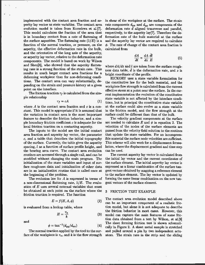
implemented with the contact area fraction and as- perity lay vector as state variables. The contact area evolution model is taken from Korzekwa et al.[7]. This model calculates the fraction of the area that is in boundary contact from a rate of flattening of the surface asperities. The flattening rate (l/E) is a function of the normal traction, or pressure, on the asperity, the effective deformation rate in the bulk, and the orientation of the long axis of the asperity, or asperity lay vector, relative to the deformation rate components. The model is based on work by Wilson and Sheu[8], who showed that the asperity flatten- ing rate is a strong function of the strain rate. This results in much larger contact area fractions for a deforming workpiece than for non-deforming condi- tions. The contact area can vary substantially, de- pending on the strain and pressure history at a given point on the interface.

The friction traction ~f is calculated from the sim- ple relationship

where A is the contact area fraction and c is a con- stant. This model is appropriate if it is assumed that the variation in contact area is the most important feature to describe the friction behavior, and a sim- ple boundary friction coefficient c is adequate for the local friction traction on a contacting asperity.

The inputs to the model are the initial contact area fraction and asperity lay vector, the parameter c, and a table that describes the initial topography of the surface. Currently, the table gives the asperity spacing, I as a function of surface profile height, and the bearing area curve. The contact area evolution routines are accessed through a single call, and can be modified without changing the main program. The initialization of the state variables and input of sur- face roughness data and initialization of other data are in an initialization routine that is called once at the beginning of the problem.

The evolution law for A is expressed in terms of a non-dimensional flattening rate, 1/E. The evalu- ation of E uses several external variables that must be obtained at each point on the surface where the friction traction is required. The function

~f = CA (1)

is evaluated from a lookup table, where

H = 5 k (3)

and 4 = tan-l(d,,/d,,) (4)

The normal traction applied by the tool to the sur- face of the workpiece is T,, and k is the flow strength

in shear of the workpiece at the surface. The strain rate components d,, and d,, are components of the deformation rate d aligned transverse and parallel, respectively, to the asperity lay[7]. Therefore the d e formation rate of the bulk material at the surface and the asperity lay vector are required to calculate 4. The rate of change of the contact area fraction is calculated from

dA dAd1 dt dz E

where dA/dz and I are taken from the surface rough- ness data table, d is the deformation rate, and z is height coordinate of the profile.

HICKORY uses a state variable formulation for the constitutive law for the bulk material, and the workpiece flow strength is calculated from the current effective stress at a point near the surface. In the cur- rent implementation the evolution of the constitutive state variable is not affected by the interface condi- tions, but in principal the constitutive state variable at the surface could also evolve as a state variable in the friction model, and the flow strength at the surface could be different than that of the bulk.

The velocity gradient components at the surface are needed to calculate E and 4 in equation 2. The velocities of the nodes of the surface elements are passed from the velocity field solution to the routines that update the state variables. For an incompress- ible material the surface node velocities are sufficient. This scheme will also work for a displacement formu- lation, where the displacement gradient and time step can be used.

The current asperity lay vector is calculated from the initial lay vector and the current coordinates of the surface element. The initial asperity lay vector is expressed as a linear combination of the surface tan- gent vectors obtained by mapping a reference element to the surface element. The lay vector is updated by forming the same linear Combination on the new tan- gent vectors of the surface element.

(5) -= - -

3 FRICTION TEST EXAMPLE

The contact area evolution model described above can be an important component of a realistic fric- tion model, but alone it is not adequate to describe the friction behavior in most cases. However, this model can capture the main features of some fric- tion data obtained from a test by Wilson, et al.[9] The sheet forming friction test is shown schemati- cally in Figure 2. A sheet metal sample is stretched and pulled around a pin by two independent actu- ators. The strain rate in the strip and the sliding

F2

t Sheet Forming Simulator

Figure 2: Sheet forming friction test.

velocity at the interface between the strip and pin can be controlled independently.

This experiment can separate the effects of normal pressure, sliding velocity and plastic strain by varying the angle of wrap and actuator velocities. Saha and Wilson[lO] showed that for some materials the ap- parent coefficient of friction at the interface increases with increasing strain in the sheet during the test. It

, is assumed that this is caused by the increased con- tact area fraction due to asperity flattening by the mechanism described in the previous section. The fractional contact area at each point on the work- piece surface in contact with the tool will depend on the strain and normal traction history of that point.

The sheet forming friction test was modeled as a plane strain problem with either the contact area evolution model for friction or with Coulomb friction. The Coulomb model used the relationship

Tf = W n (6)

where T~ is the normal traction. Figure 3 shows a region of the mesh for a test with a 90 degree wrap angle. The results presented here are for an average strain rate of either 0.07/s or 0.105/s, and an aver- age sliding velocity of x llmm/s. The material and surface properties were for a type 304 stainless steel sheet. The asperity lay was defined as perpendicular to the sliding and stretching direction, and therefore it did not evolve for the examples shown here. This results in a constant value of for the flattening rate calculation.

For the state variable model, the contact area

Figure 3: Sheet forming friction test finite element model.

fraction is initialized to 0.04, and at the beginning of the test the friction traction is very low. As the sheet sample is stretched while in contact with the tool, the contact area increases, and the friction trac- tion increases. Figure 4 shows the contact area state variable at various times during the test. The posi- tion coordinate is the distance along the strip surface from one end of the sample, and only a portion of the surface is in contact with the tool at any time.

As the test proceeds, points on the workpiece sur- face that were initially in contact with the tool will have the contact area increase until they leave con- tact. When the problem has progressed to the point where the strip surface at the beginning of the contact region has traveled along the complete tool-workpiece interface and come out of contact, the state variable distribution reaches an approximate steady state. If the workpiece is hardening with strain this will not be strictly true, because of the influence of the workpiece flow strength on the normal traction.

At a time of 1.6 sec it can be seen in Figure 4 that the contact area distribution has evolved to this steady state condition at the interface. The region of contact is to the right of the peak. The contact area at a point on the strip increases monotonically as the point proceeds along the contact region, and stops increasing after it leaves the tool. The flat region on the peak is the portion of the strip that has traveled the full length of the contact region and developed the maximum contact area fraction.

For relatively low friction tractions, the contact area model and the Coulomb model give very similar normal traction distributions at the interface. Figure

0.45 1

0.4 - .O 0.35 -

0.3 - 0.25 -

c 0

U

- 4 0.2 -

3 0.1 - 5 0.15 -

0.05 -

0.1 sec - 0.4 S m ------ 1.6sm -

p-.,,-,, \ Sliding 30

25

- 20 15

a" - b OJO 40 50 60 70 80 -= 10

910 g Position (mm) b 5

0 Figure 4 Contact area fraction evolution.

5 shows the normal tractions for both models at the same three times as Figure 4. The Coulomb coeffi- cient was 0.1, and c was 10.25 MPa for the contact area model. The tangential traction distributions, however, are quite different, as shown in Figure 6. The friction traction for the Coulomb model is nearly constant as would be expected based on the nearly constant normal traction. The results for the contact area model reflect the contact area evolution along the interface, giving an increasing friction traction as a material point proceeds along the interface.

The increase in friction traction with increasing strain rate is shown in Figure 7. The contact area fraction increases for the higher strain rate because the accumulated strain while in contact with the tool is higher for a given point on the surface of the sheet. When the results are expressed as an average fric- tion coefficient, defined as the normal load divided by tangential load, the apparent coefficient of fric- tion increases with strain rate, as observed in the experiment. The Coulomb model does not capture this effect since, by definition, the ratio of normal to tangential tractions is constant.

4 DISCUSSION

Some of the results from the finite element model of the sheet forming friction test are given in Table 1 for an average sliding velocity of = llmm/s and av- erage strain rate of 0.07/s. The loads on the ends of the strip and the geometry were used to calculate the average normal traction P and average friction coef- ficient ji, after the method that was used to analyze the experiments in [lo].

I , I , I I , I I I

Coulomb -

35 40 45 50 55 60 65 70 75 80 85 Position (mm)

-5

Figure 5: Normal traction at the interface for Coulomb and contact area models.

Table 1: Average Friction Coefficients for Coulomb and Contact Area Friction Models

t Strain rate = 0.105.

Coulomb - Contact Area ---- F

1 -1 V

-2 i 60 65 70 75 80 55

Position (mm)

Figure 6: Comparison of tangential (friction) trac- tions for Coulomb and contact area models.

In order to match a typical experimental result of p = 0.1 values of c and /.L were chosen to be 10.2 MPa and 0.1, respectively, for the two friction models in the finite element simulations. Doubling both /.L and c gives p x 0.2 for both models, and one can argue that the two models cannot be distinguished because p varies linearly with both /I and c over this range of observed values of p. However, the value of p increases by ~10% when the strain rate is increased from 0.07/s to 0.105/s when the contact area model is used. This is approximately the same increase that was experimentally observed in [lo] for a galvanized sheet steel. At higher friction levels the two models do not agree as closely. When the Coulomb coefficient is set to 0.4, the value of ,ti is calculated to be 0.45, while the comparable value for the contact area model is 0.41.

These results illustrate the limitations of using ei- ther experiments or simulations alone. Experiments usually only measure average tractions, and do not resolve the spatial variation in conditions at the in- terface. The sheet forming friction test cannot distin- guish between the two results in Figure 6 with a single test, because the average friction coefficients are the same. On the other hand, a numerical Simulation can generate very detailed results, and numerical exper- iments are possible that cannot be conducted in the physical world. However, the numerous limitations of the simulation tools and their underlying physical models make it impossible to independently verify the correctness of a given friction model using simulations alone.

A combined approach seems best, where the can-

I Strain rate 1.05 -

-I 60 65 70 75 80 85

Position (mm)

Figure 7: Fkiction tractions for two strain rates using the contact area model.

didate models are chosen based on experimental re- sults, and simulations are used to validate them. Sim- ulations can then be used to predict the results of sub- sequent experiments, and the results will provide fur- ther validation or expose the limitations of the model. Experimental characterization to try to identify fric- tion and wear mechanisms must be used to ensure that the various friction models are used appropri- ately. If a complex model for friction is to be incor- porated into a finite element code and used to model complex forming operations, it must be validated for simple problems before it can be useful.

The contact area evolution model shown here will be used as part of more sophisticated models cur- rently under development. In most cases a liquid lubricant is present, and the hydrodynamics of the lubricant film will have a very strong effect on the actual contact area[ll]. The flattening model used is probably reasonable for some materials, but in other cases the surface will roughen as it is strained, and this will have a very strong effect on the actual con- tact area. Also, the coefficient c encompasses com- plex boundary friction behavior that depends on the composition of the lubricant, the tool and the work- piece, as well as roughness features. In some cases a model for boundary friction must be added to capture the important effects.

for state variable friction models is flexible enough to accommodate a wide range of physically-based mod- els. Even if the mechanisms are not understood com- pletely, empirical models can be implemented in terms of physically meaningful quantities.

The general implementation method described here

The state variable structure presented here may not be adequate for the implementation of some mod- els involving hydrodynamic lubrication theory. The method described here allows evolution of state vari- ables based on local variables on a point-by-point basis. Much of the current theory of hydrodynamic effects involves integration of the Reynolds equation along the interface to find the lubricant film thickness and pressure distribution. The theory is very attrac- tive and can provide valuable predictions of friction behavior, but a different approach to implementation is required. An example of this type of lubrication model in a finite element code has been demonstrated by Liu et al.[12]

5 CONCLUSIONS

A state variable friction model has been implemented into the finite element code HICKORY. This imple- mentation is sufficiently general to allow a wide range of physical phenomena at the tool-workpiece inter- face to be incorporated into metal deformation pro- cess simulations. A contact area evolution model for friction was employed in a simulation of a friction test for sheet forming. It was demonstrated that the con- tact area model can capture experimental effects that cannot be modeled by simple Coulomb friction.

It is proposed that numerical simulations be used to help analyze friction experiments and evaluate fric- tion models. It seems likely that a combination of experiments and simulation will further the under- standing of the basic friction mechanisms, as well as validate the friction model for use in complex metal forming simulations. The ability to use more realistic, physically based friction models promises to make nu- merical simulations of metal forming processes more accurate and useful.

6 ACKNOWLEDGMENTS

This work was supported by the Department of En- ergy under contract W-7405-ENG-36. Thanks go to to Paul Dawson at Cornel1 University and Bill Wil- son at Northwestern University for their helpful dis- cussions and encouragement.

REFERENCES

(31 N. Bay and T. Wanheim, “Real area of contact and friction stress at high pressure sliding contact,” Wear, vol. 38, pp. 201-209, 1976.

[4] W.R.D. Wilson, “Friction models for metal forming in the boundary lubrication regime,” mans. ASME Journal of Engineering Materials and Technology, vol. 113, pp. 60-68, 1991.

[5] W.R.D. Wilson, “Strategy for friction modeling in computer simulations of metalforming,” in Proc.

[6] G.M. Eggert and P.R. Dawson, “Assessment of a thermoviscoplastic model of upset welding by com- parison to experiment,” International Journal of Mechanical Sciences, vol. 28, pp. 563-589, 1986.

[7] D.A. Korzekwa, P.R. Dawson, and W.R.D. Wilson, “Surface asperity deformation during sheet form- ing,” International Journal of Mechanical Sciences,

[8] W.R.D. Wilson and S. Sheu, “Real area of con- tact and boundary fiction in metal forming,” In- ternational Journal of Mechanical Sciences, vol. 30, pp. 475489, 1988.

[9] W.R.D. Wilson, H.G. Malkani, and P.K. Saha, “Boundary friction measurements using a new sheet metal forming simulator,” in Proceedings of NAMRC

[lo] P.K. Saha and W.R.D. Wilson, “Influence of plas- tic strain on friction in sheet metal forming,” Wear,

[ll] W.R.D. Wilson and D. Chang, “Low speed mixed lubrication of bulk metal forming processes,” in 2 5 - bology in Manufacturing Processes (K. Dohda, S . Jahanmir, and W.R.D. Wilson, eds.), TFUB-Vol.5, (New York, NY), pp. 159-167, ASME, ASME, 1994.

[12] W.K. Liu, Y-K Hu, and T. Belytschko, “ALE finite elements with hydrodynamic lubrication for metal forming,” Nuclear Engineering and Design, vol. 138,

NAMRC XVI, pp. 45-84, SME, 1988.

VO~. 34, pp. 521-539, 1992.

XIX, pp. 37-42, SME, SME, 1991.

V O ~ . 172, pp. 167-173, 1994.

pp. 1-10, 1992.

[l] J.A. Schey, Tbibology in Metalworking. American . Society for Metals, 1983.

[2] W.R.D. Wilson, “Friction and lubrication in bulk metal forming processes,” Journal of Applied Metal- working, vol. 1, pp. 7-19, 1979.